Scandium abundances of F-G-K dwarf stars in a wide metallicity range

Institute of Astronomy, Russian Academy of Sciences, Pyatnitskaya st. 48, 119017 Moscow, Russia¹

A new model atom of Sc II was constructed using the most up-to-date atomic data. For the testing purpose, the non-local thermodynamic equilibrium (non-LTE) calculations were carried out for three stars with reliably determined atmospheric parameters: the Sun, HD 61421 (Procyon), and HD 84937. Accounting for deviations from LTE leads to smaller abundance errors compared with the LTE case and consistent within the error bars abundances obtained from different Sc II lines. Solar non-LTE abundance $\log\varepsilon_{\rm Sun}=3.12\pm 0.05$ exceeds the meteoritic abundance recommended by Lodders (2021), by 0.08 dex. But agreement within 0.02 dex with the meteoritic abundance is obtained for Procyon. Using high-resolution spectra, we determined the scandium LTE and non-LTE abundances for 56 stars in the metallicity range $-2.62\leq$ [Fe/H] $\leq$ 0.24. The dependence of [Sc/Fe] on [Fe/H] demonstrates a similarity with the behavior of the $\alpha$-process elements: scandium is enhanced relative to iron ([Sc/Fe] $\sim$ 0.2) for [Fe/H] $<-1$, and [Sc/Fe] decreases with increasing [Fe/H] for the higher metallicity. There is a hint of a tight relation between abundances of scandium and titanium. The results obtained provide observational constraints to the scenarios of scandium origin.

Key words: stellar atmospheres, non-LTE line formation, abundances of scandium in stars

 
^∗ e-mail $<$lima@inasan.ru$>$

1 Introduction

There are several problems associated with the stellar scandium abundances.

The determinations of the Sc abundance in the solar atmosphere give values that differ from each other by more than 2$\sigma$: from $\log\varepsilon_{\rm Sun}$ = 3.07$\pm$0.04 (Zhang et al.,, 2008) to $\log\varepsilon_{\rm Sun}$ = 3.16$\pm$0.04 (Scott et al.,, 2015) and exceed the meteoritic abundance $\log\varepsilon_{\rm met}$ = 3.04$\pm$0.03 (Lodders,, 2021). Hereafter, an abundance scale is used in which $\log\varepsilon$(H) = 12.

Scandium exhibits different behavior in A-type stars with iron abundances close to solar ([Fe/H] $\sim$ 0, normal A stars), and non-magnetic A stars with strong metal lines (Am stars, [Fe/H] $\succsim$ 0.5). But Sc does not belong to the group of metals with strong lines. On the contrary, Am stars reveal a deficit of Sc, which can reach an order of magnitude (Adelman et al. 2000 and references in their article). Therefore, the scandium abundance plays a key role in classifying a star as Am. However, the reasons for the different behavior of Sc and elements of the Fe group in A-type stars remain unclear.

An origin of Sc remains unclear. According to the most recent models of the chemical evolution of the Galaxy (Kobayashi et al.,, 2020), the main source of Sc during the life of the Galaxy were type II supernovae (SNeII) and hypernovae (HN), but they produced scandium an order of magnitude less than is observed in the Galactic matter. The observational data on the Sc abundance of stars in a wide range of metallicity serves to test the assumptions made in the Galactic chemical evolution model and establish constraints to the model parameters. In the literature, we find determinations of the Sc abundance in large samples of stars with very low Fe abundances ([Fe/H] $<-2$), for example, works by Cayrel et al., (2004), Yong et al., (2013), Roederer et al., (2014), but there are very few data for stars with [Fe/H] $>-2$. Zhao et al. (2016) obtained the Sc abundance for 49 dwarf stars in the range $-2.6\leq$ [Fe/H] $\leq 0.25$ and Reggiani et al. (2017) for 23 stars with [Fe/H] between $-2.8$ and $-1.5$.

In this paper, two of the mentioned problems are considered, namely, those concerning the Sun and the Galactic trend [Sc/Fe] – [Fe/H]. The problem of scandium in normal A stars and Am stars will be the subject of our next article. We determine the solar Sc abundance from lines of Sc II using the most up-to-date atomic data and a line-formation modeling free from the simplifying assumption of local thermodynamic equilibrium (LTE). It is referred to as the non-LTE approach. It is important to find an answer to the question of whether the solar atmosphere Sc abundance represents the cosmic one or whether there are physical processes that change the Sc abundance of the Sun in comparison with the meteoritic abundance.

Second, we revise the Sc abundance of the sample of stars from Zhao et al. (2016) using a new model of the scandium atom and abandoning the differential approach. Zhao et al. (2016) determined [Sc/H] = $\log\varepsilon_{\rm star}-\log\varepsilon_{\rm Sun}$ for each individual line in order to exclude the influence of errors in the oscillator strengths (or $gf$-values) on the final result. This was a forced approach due to the lack of precise atomic parameters of the lines, but it excluded from the analysis the Sc II lines in range 4246-4420 Å due to strong blending effects in the solar spectrum. Exactly these lines are most reliably measured in stars with [Fe/H] $<-2$. As a result, for very metal-poor (VMP, [Fe/H] $<-2$) stars, Zhao et al. (2016) were able to use only two to three lines, and the Sc abundance was not determine for two VMP stars. In our work, we used laboratory measurements of $gf$ from Lawler et al. (2019). Therefore, for each star, the abundance was determined for all observed lines of Sc II. To improve statistics in the range $-1.5<$ [Fe/H] $<-1$, the stellar sample was complemented by five stars from Mashonkina et al. (2003).

To solve the tasks posed, a model atom of Sc II was constructed using the transition probabilities from Lawler et al. (2019) and the electron collision rates from Grive and Ramsbottom (2012). Earlier, the non-LTE method for Sc I–Sc II was developed by Zhang et al. (2008) and applied by Zhao et al. (2016) to determine stellar non-LTE abundances.

The paper is structured as follows. The new model atom is presented in Section 2. It is tested in Section 3 by analyzing the Sc II lines in the spectra of stars with reliably determined atmospheric parameters, that is the Sun, HD 61421 (Procyon), and HD 84937. In Section 4, we determine the scandium LTE and non-LTE abundances of the sample stars and analyze the resulting trend [Sc/Fe] – [Fe/H]. Finally, we summarize our conclusions and recommendations.

2 New model of the scandium atom

2.1 Atomic data

Energy levels. The atom model includes three lower terms of Sc I, 888 energy levels of Sc II and the ground state of Sc III. The level energies are taken from the NIST database (Kramida et al. 2019) and the atomic structure calculations by Kurucz (2009). With ionization energy $\chi$ = 6.54 eV, scandium is strongly ionized in the atmospheres of stars with an effective temperature of $T_{\rm eff}$ $>$ 4500 K, and a number density of Sc I depends strongly on the accuracy of calculations of the ionization and recombination rates. In the absence of accurate photoionization cross sections and collisional processes, we exclude the possibility of an accurate calculation of the statistical equilibrium (SE) of Sc I. For the constraint of particle conservation, it suffices to have the three most populated lower terms of Sc I.

Figure 1: Sc II levels, included in the model atom, and the transitions corresponding to the spectral lines, used in abundance determinations. Solid and dashed horizontal lines indicate the energy of even and odd superlevels, respectively. Levels with violation of the LS-coupling are presented in column ’e’.

The fine splitting is taken into account for the Sc II $3d4s\,^{3}{\rm D}$ ground state and the low-excitation term $3d^{2}\,{}^{3}{\rm F}$. High-excitation levels of Sc II with a small energy separation and of the same parity were combined. Such superlevels were constructed from the levels predicted in the atomic structure calculations, but not discovered (so far) in lab measurements. The average energy of the combined superlevel was calculated taking into account the statistical weights of individual levels. The final model atom includes 79 even and 55 odd levels of Sc II. The highest levels of Sc II are separated from the ground state of Sc III by 0.08–0.26 eV, which is much lower than the average kinetic energy of electrons at temperatures of up to 20 000 K. This ensures effective coupling of the Sc II levels with the ground state of Sc III through collisions. The term diagram is shown in Fig. 1.

Radiative rates. The model atom includes 4032 allowed bound-bound (b-b) transitions. $gf$-values are taken from Lawler et al. (2019) and Kurucz (2009). For the Sc II transitions, which are associated with the low-excitation levels and in which the upper levels can be pumped by ultraviolet (UV) radiation, the radiative rates are calculated using the Voigt function for the absorption profile. For other transitions, the Doppler absorption profile is adopted. The photoionization cross sections are calculated in the hydrogenic approximation using the effective principal quantum number instead of the principal quantum number. Note that the number density of Sc II practically does not depend on the accuracy of calculations of the ionization/recombination rates, since Sc II is the dominant ionization stage in the atmospheres of the studied objects.

Collision rates. In the atmospheres of late spectral type stars, the number density of electrons is much lower than the number density of neutral hydrogen atoms; therefore, the excitation of levels and the formation of ions can occur as a result of collisions not only with electrons, but also with H I atoms. For electron-impact excitation, we use data from Grieve and Ramsbottom, (2012) obtained with the R-matrix method. They are available for 948 b-b transitions of Sc II between levels with an excitation energy of $E_{\rm exc}$$\leq$ 9.5 eV. Note that all the observed lines of Sc II are formed between levels in this energy interval. For the remaining b-b transitions, electronic collisions are calculated using the van Regemorter (1962) formula if the transition is allowed, and an effective collision strength is assumed to be 1 if the transition is forbidden. Electron-impact ionization rates are calculated using Seaton’s (1962) formula and the adopted photoionization cross sections at the threshold.

To account for collisions with H I, leading to excitation of Sc I and Sc II, we use the Steenbock and Holweger (1984) formula. Since the formula is approximate, with an accuracy of only the order of magnitude, the calculations were made with several values of the scaling factor $S_{\!\rm H}$ = 0, 0.1 and 1.

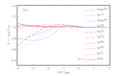
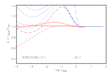
Figure 2: b-factors of the selected levels of Sc II in the model atmospheres 5780/4.44/0 and 6350/4.09/$-2.1$.

2.2 Statistical equilibrium of Sc II in stellar atmospheres of different metallicity

The system of the statistical equilibrium equations and radiative transfer in a given atmospheric model is solved using the code DETAIL developed by Giddings, (1981) and Butler, (1984) based on the accelerated $\Lambda$-iteration method (Rybicki and Hummer,, 1991, 1992). The opacity package was updated by T. Gehren, J. Reetz, L. Mashonkina, as described in Mashonkina et al. (2011).

Throughout this work, we use plane-parallel (1D) atmospheric models from the MARCS database (Gustafsson et al. 2008). The models with given $T_{\rm eff}$, surface gravity log $g$ and [Fe/H] were obtained by interpolation using the algorithm posted on the MARCS website.

Figure 2 shows b-factors, b = $n_{\rm NLTE}/n_{\rm LTE}$, of individual levels of Sc II, related to the observed lines, in the model atmospheres with solar metallicity ($T_{\rm eff}$/log $g$/[Fe/H] = 5780/4.44/0) and with a large deficiency of metals (6350/4.09/$-2.1$). Here, $n_{\rm NLTE}$ and $n_{\rm LTE}$ are the level populations obtained by solving the SE equations (non-LTE) and by the Boltzmann-Saha formulas (LTE). Since in both models Sc II is the dominant ionization stage, then the populations of its ground state $3d4s\,^{3}{\rm D}$ and the first excited level $3d4s\,^{1}{\rm D}$ ($E_{\rm exc}$ = 0.3 eV) are close to the LTE populations (b $\simeq$ 1) everywhere in the atmosphere. Since the intensity of UV radiation is higher in a hotter and metal-poor atmosphere, the radiative pumping of the odd terms $3d4p\,^{3}{\rm F}^{\circ}$, $3d4p\,^{3}{\rm P}^{\circ}$ and $4s4p\,^{3}{\rm P}^{\circ}$ via transitions from the ground state (lines 3613-3642 Å, 3361-3372 Å and 2552-2563 Å) is more efficient in the 6350/4.09/$-2.1$ model. Therefore the behavior of all levels above $E_{\rm exc}$ = 0.3 eV differs in the two models. In the 6350/4.09/$-2.1$ model, already in deep layers, the medium becomes optical thin for radiation in the spontaneous transitions from overpopulated (b $>$ 1) odd terms to the low-excitation levels, which makes the populations of the latter also higher than the LTE ones, although to a lesser extent than those of the upper levels. An example is the transition $3d^{2}\,{}^{3}{\rm P}$ – $3d4p\,^{3}{\rm P}^{\circ}$, in which the 5641 Å line is formed.

3 Sc II lines in spectra of the Sun, Procyon, and HD 84937

In order to test the new model atom, we analyzed lines of Sc II in the three reference stars for which there are high-resolution spectra and the atmospheric parameters are reliably determined. These are the Sun, the star HD 61421 (Procyon, F5 IV-V) with a metallicity close to the solar one, and a VMP star HD 84937.

3.1 Observational material and atmospheric parameters

We analyze the spectrum of the Sun as a star using the atlas of Kurucz et al. (1984). Spectral resolving power is R = $\lambda/\Delta\lambda\simeq$ 300000. As in our previous studies, we use the well-known parameters of the solar atmosphere: $T_{\rm eff}$ = 5780 K, log $g$ = 4.44, and a microturbulence velocity of $\xi_{t}$ = 0.9 km s^-1.

Spectrum of Procyon obtained with R $\simeq$ 80 000 was taken from the UVESPOP archive (Bagnulo et al.,, 2003). Atmosphere parameters $T_{\rm eff}$ = 6615 K, log $g$ = 3.89, [Fe/H] = $-0.05$, and $\xi_{t}$ = 2 km s^-1 were determined by Ryabchikova et al. (2016) by automatically fitting the theoretical spectrum to the selected regions in the same observed spectrum. Note that $T_{\rm eff}$ = 6615 K agrees within the determination error (89 K) with the effective temperature obtained by Boyajian et al. (2013) in the range from 6562 K to 6597 K based on interferometric measurements of Procyon’s angular diameter.

The observed spectrum (R $\simeq$ 80 000) HD 84937 is also taken from the UVESPOP archive (Bagnulo et al.,, 2003). In addition, we use the ultraviolet spectrum obtained on the Hubble Space Telescope with the STIS spectrograph in the range of 1875-3158 Å, with a resolution of R $\simeq$ 25 000. This data is provided by Thomas Ayres on the ASTRAL project website. Atmospheric parameters $T_{\rm eff}$ = 6350 K, log $g$ = 4.09, [Fe/H] = $-2.16$, and $\xi_{t}$ = 1.7 km s^-1 were determined by Sitnova et al. (2015) using spectroscopic and photometric methods and a known distance.

3.2 Determination of scandium abundances

Table 1: Atomic parameters of the Sc II lines and the LTE and non-LTE (NLTE, $S_{\!\rm H}$ = 0.1) abundances of scandium ($\log\varepsilon$) for the reference stars.

$\lambda$, Å	$E_{\rm exc}$,	log $gf$	Sun		Procyon		HD 84937
	eV		5780/4.44/0		6615/3.89/$-0.01$		6350/4.09/$-2.16$
			LTE	NLTE	LTE	NLTE	LTE	NLTE
2552.351	0.022	0.05	-	-	-	-	0.99	1.23
2563.19	0.000	–0.57	-	-	-	-	0.98	1.15
3353.72	0.315	0.26	-	-	-	-	1.03	1.13
3359.68	0.008	–0.75	-	-	-	-	1.09	1.16
3368.94	0.008	–0.39	-	-	-	-	1.09	1.18
3567.70	0.000	–0.47	-	-	-	-	1.07	1.15
3576.34	0.008	0.01	-	-	-	-	1.01	1.10
3580.92	0.000	–0.14	-	-	-	-	1.07	1.16
3589.63	0.008	–0.57	-	-	-	-	1.10	1.17
3590.47	0.022	–0.55	-	-	-	-	1.11	1.17
3613.83	0.022	0.42	-	-	-	-	1.07	1.11
3642.78	0.000	0.05	-	-	-	-	1.05	1.13
3645.31	0.022	–0.41	-	-	-	-	1.13	1.18
4246.82	0.315	0.24	-	-	-	-	1.14	1.22
4314.08	0.618	–0.11	3.22	3.15	3.17	3.05	1.15	1.27
4320.73	0.605	–0.28	-	-	-	-	1.16	1.27
4325.00	0.595	–0.44	-	-	-	-	1.14	1.25
4400.38	0.605	–0.54	3.18	3.16	3.13	3.07	1.17	1.26
4420.66	0.618	–2.33	3.18	3.18	3.08	3.07	-	-
4670.40	1.357	–0.60	3.14	3.11	3.12	3.08	1.11	1.20
5031.02	1.357	–0.41	-	-	-	-	1.16	1.26
5239.81	1.455	–0.76	3.13	3.13	3.08	3.09	-	-
5357.201,2	1.500	–2.11	3.15	3.15	3.04	3.06	-	-
5526.77	1.768	–0.01	3.24	3.16	3.21	3.09	1.17	1.29
5640.99	1.500	–0.99	3.14	3.13	3.08	3.06	-	-
5657.88	1.507	–0.54	3.20	3.18	3.14	3.09	1.08	1.24
5658.35	1.497	–1.17	3.15	3.15	-	-	-	-
5669.04	1.500	–1.10	3.11	3.11	-	-	-	-
5684.19	1.507	–1.03	3.15	3.14	3.09	3.07	-	-
6245.623	1.500	–1.02	3.04	3.03	3.01	2.99	-	-
6279.74	1.500	–1.33	3.14	3.13	-	-	-	-
6300.683	1.510	–1.90	2.99	3.00	3.04	3.02	-	-
6320.833	1.500	–1.82	3.06	3.05	3.04	3.03	-	-
6604.58	1.357	–1.26	3.08	3.09	2.99	3.00	-	-
Mean			3.14	3.12	3.09	3.06	1.09	1.19
$\sigma$(dex)			0.06	0.05	0.06	0.03	0.06	0.06
1 no HFS; 2 $gf$ (Lawler and Dakin,, 1989); 3 $gf$ (Kurucz,, 2009).

Lines of Sc II, used in abundance determinations, together with their atomic parameters are listed in Table 1. We use oscillator strengths based on laboratory measurements of Lawler et al., (2019). Exceptions are the Sc II 5357 Å line with log$gf$ measured by Lawler and Dakin (1989) and the lines at 6245, 6300 and 6320 Å, for which there are only calculations by Kurucz (2009).

The levels in scandium atoms and ions are subject to hyperfine splitting (HFS). Therefore, in calculating the theoretical line profiles, it is necessary to take into account their HFS structure. For all studied lines, except for Sc II 2552 Å and 5357 Å, wavelengths and oscillator strengths of the HFS components are available in the updated VALD database (Pakhomov et al. 2019), as well as on the page https://github.com/vmplacco/linemake. We note the complete agreement of the data in these two sources. In the solar spectrum, the Sc II 5357 Å line has an equivalent width of $EW\simeq$ 5 mÅ, and neglecting the HFS structure does not affect the theoretical $EW$ and derived abundance. Sc II 2552 Å was measured only for HD 84937. Possibly, due to neglecting the HFS structure, it gives an abundance that is 0.08 dex higher than the average for other UV lines.

Van der Waals damping constants, log $\Gamma_{6}$, for lines of Sc II were calculated by Kurucz, (2009) and presented in the VALD database (Ryabchikova et al.,, 2015; Pakhomov et al.,, 2019). They have close values for different lines and, per 10 000 K, range from log $\Gamma_{6}=-7.81$ to log $\Gamma_{6}=-7.83$.

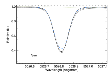
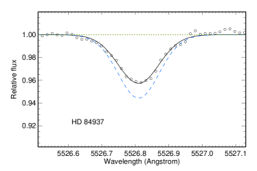
Figure 3: Sc II 5526 Å in the spectra of the Sun and HD 84937 (circles) and the best non-LTE fits ($S_{\!\rm H}$ = 0.1, solid curve). The dashed curves corresponds to the LTE calculations. For the Sun and HD 84937, calculations were made using $\log\varepsilon$ = 3.16 and 1.29, respectively.

The codes and methodology for abundance determinations. Everywhere in this study, the synthetic spectrum method is applied by automatically fitting the theoretical line profile to the observed one. Equivalent widths were measured in the same procedure only for the purpose of illustrating the results. We use the codes synthV_NLTE (Tsymbal et al., 2019) and BinMag (Kochukhov,, 2018). The list of lines for calculating the synthetic spectrum is taken from VALD. In addition to the model atmosphere, microturbulent velocity, and line atomic parameters, the spectral resolving power and the projection of the rotation velocity onto the line of sight $V\sin i$ were the fixed parameters in the procedure for matching the theoretical and observed spectra. For the Sun and Procyon, $V\sin i$ = 1.8 km s^-1 and 4 km s^-1, respectively. As in Zhao et al. (2016), rotational broadening was also taken into account for six stars with $V\sin i\geq$ 6 km s^-1: HD 58855 ($V\sin i$ = 10 km s^-1), HD 89744 (9 km s^-1), HD 92855 (10 km s^-1), HD 99984 (6 km s^-1), HD 100563 (10 km s^-1), HD 106516 (7 km s^-1). For the rest of the studied stars, line broadening due to rotation was not taken into account, since it is much smaller than the broadening due to macroturbulent motions. Macroturbulent velocity $V_{\rm mac}$, scandium abundance, and wavelength shift of the line were free parameters in the fitting procedure. The Doppler shift, due to the radial velocity of the star and the orbital motion of the Earth around the Sun, was in advance taken into account. Figure 3 displays the best non-LTE fits of Sc II 5526 Å in the Sun and HD 84937, as examples.

Non-LTE effects on lines of Sc II. For comparison, Fig. 3 shows the LTE profiles calculated with the abundance obtained in the non-LTE calculations. For the Sun, departures from LTE lead to slight strengthening Sc II 5526 Å, and, on the contrary, to weakening for HD 84937. Sc II 5526 Å is formed in the transition $3d^{2}\,{}^{1}{\rm G}$ – $3d4p\,^{1}{\rm F}^{\circ}$. In the solar atmosphere, its core is formed at depths with log $\tau_{5000}\sim-1.6$, where a population of the lower level is close to the LTE one, while the upper level is underpopulated (Fig. 2). As a result, the line source function is less than the Planck function at these depths, and the line is strengthened. The difference between non-LTE and LTE abundances, $\Delta_{\rm NLTE}$ = $\log\varepsilon_{\rm NLTE}-\log\varepsilon_{\rm LTE}$, which is called the non-LTE abundance correction, is $-0.08$ dex in this case. In the atmosphere of HD 84937, the core of Sc II 5526 Å is formed at depths with log $\tau_{5000}\sim-0.1$, where the population of the lower level is close to the LTE one, while the upper level is overpopulated (Fig. 2), which leads to a weakening of the line. The non-LTE correction is positive and equal to $\Delta_{\rm NLTE}$ = 0.12 dex.

The obtained LTE and non-LTE abundances from individual lines are presented in Table 1 and in Fig. 4 for each of the three reference stars. For the Sun, the non-LTE abundance corrections are negative and small in absolute value. Exception is Sc II 6604 Å with a small positive correction. Procyon is hotter, and the negative non-LTE corrections are larger in absolute value. HD 84937 reveals stronger non-LTE effects in the Sc II lines, since the intensity of UV radiation is higher and the electron number density is lower, resulting in higher radiative rates and lower collisional rates. Lines of Sc II are weaker in non-LTE than in LTE, and $\Delta_{\rm NLTE}$ are positive. For each of the stars non-LTE leads to a smaller dispersion in the single line measurements around the mean $\sigma=\sqrt{\sum(x-\bar{x})^{2}/(N_{l}-1)}$, where $N_{l}$ is the number of lines. It is, in particular, well seen for Procyon, where $\sigma$ decreases by a factor of two, to 0.03 dex, and for HD 84937, where non-LTE removes the abundance difference between the lines in the UV and visible regions. Figure 5 illustrates the reliability of abundance determination from Sc II 2563 Å in the spectrum of HD 84937. The Sc II line is located in the far wing of Fe I 2563.399 Å ($E_{\rm exc}$ = 0.96 eV, log $gf=-2.26$), which is well reproduced for given atomic parameters and iron abundance, and blends with Cr II 2563.157 Å ($E_{\rm exc}$ = 6.805 eV, log $gf=-1.683$), which is much weaker than Sc II 2563 Å and, due to the uncertainty in the Cr abundance (or $gf$), can affect the derived Sc abundance by no more than 0.01 dex.

Influence of collisions with hydrogen atoms. Non-LTE calculations were carried out for three variants of collisional rates in the SE equations: $S_{\!\rm H}$ = 0 – pure electron collisions; $S_{\!\rm H}$ = 1 – collisions with hydrogen atoms are accounted for with the formula of Steenbock and Holweger (1984); $S_{\!\rm H}$ = 0.1 – the contribution of collisions with H I is reduced by a factor of 10. For solar lines of Sc II, the non-LTE corrections range from +0.01 dex to $-0.08$ dex, if $S_{\!\rm H}$ = 0, and decrease in absolute value by a maximum of 0.01 dex in the variant $S_{\!\rm H}$ = 1. Non-LTE effects are much stronger for HD 84937, with $\Delta_{\rm NLTE}$ from 0.04 dex to 0.24 dex in option $S_{\!\rm H}$ = 0. However, collisions with H I only weakly affect the final results, namely, the difference in non-LTE abundances between variants $S_{\!\rm H}$ = 0 and 1 does not exceed 0.02 dex. Weak influence of collisions with hydrogen atoms on the magnitude of departures from LTE for the Sc II lines is due to the Sc II term structure and, possibly, the lack of exact data on the rates of these processes. The formula of Steenbock and Holweger (1984) was designed only for allowed transitions, while all the Sc II levels with $E_{\rm exc}$ $<$ 2 eV have the same parity. For allowed transitions with energies above 3 eV, radiative processes predominate over collisional ones. Hereafter, a compromise value of $S_{\!\rm H}$ = 0.1 was adopted to obtain the final non-LTE abundances.

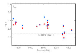
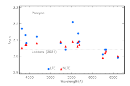
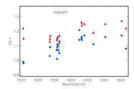
Figure 4: LTE (blue circles) and non-LTE (red triangles) abundances obtained from individual lines of Sc II in Sun, Procyon and HD 84937. The dotted line denotes the meteoritic abundance from Lodders, (2021).

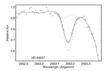
Figure 5: Sc II 2563 Å in the spectrum of HD 84937 (circles) and the best non-LTE fit (solid curve, $\log\varepsilon$ = 1.15). The dashed curve corresponds to the LTE calculations with the same Sc abundance, and the dotted curve to the calculations in the absence of Sc in the atmosphere.

The resulting solar non-LTE abundance is 0.02 dex less than the LTE value and closer to the meteoritic abundance $\log\varepsilon_{\rm met}=3.04\pm 0.03$ (Lodders,, 2021), but still exceeds it by more than 1$\sigma$. It should be noted that in different works the magnitude of meteoritic abundance varies within the error of determination. For example, Lodders et al. (2009) recommended $\log\varepsilon_{\rm met}=3.07\pm 0.02$. In Procyon, the scandium non-LTE abundance is consistent with the meteoritic value.

3.3 Comparison with the literature data

The obtained mean solar abundance agrees within the error bars with the data of other authors if the abundances from individual lines are reduced to one system of $gf$-values. Figure 6 shows the LTE abundances from individual lines as derived by Lawler et al., (2019), Zhang et al., (2008) and in this paper. Abundances of Zhang et al., (2008) were recalculated using $gf$-values, measured by Lawler et al. (2019). Differences are minimal between us and Zhang et al., (2008), since in both works the same Atlas of the Sun (Kurucz et al.,, 1984) was used and the theoretical model atmospheres, although from different sources, that is, from Gustafsson et al., (2008) and Grupp, (2004), respectively. The mean abundances agree within 0.01 dex, however, the difference reaches nearly 0.1 dex for three lines (4314, 5640, 5658 Å), which is most likely due to different treatment of blending lines.Lawler et al., (2019) used the solar disc center spectrum (Delbouille et al.,, 1973) and a semi-empirical model atmosphere (Holweger and Müller,, 1974) and obtained the higher, on average, abundance than our LTE value, by 0.02 dex.

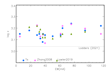
Figure 6: LTE abundances obtained from individual lines of Sc II in the solar spectrum by different authors. Circles, diamonds, and triangles correspond to this study (Ts), Zhang et al., (2008), and Lawler et al., (2019), respectively. The data of Zhang et al., (2008) were converted into the system of oscillator strengths by Lawler et al., (2019). The equivalent widths are from our measurements. The dotted line denotes the meteoritic abundance from Lodders, (2021)).

Now we discuss the original data. Using the oscillator strengths from the calculations of Kurucz, Zhang et al. (2008) obtained $\log\varepsilon$(Z08)= 3.10$\pm 0.05$ and $3.07\pm 0.04$ in LTE and non-LTE. This was the first and so far the only work on non-LTE analysis of the solar Sc II lines. Despite the improved model atom, our calculations show similar non-LTE effects for Sc II, because of their small magnitude.

Scott et al., (2015) determined the solar Sc abundance as $\log\varepsilon$(3D) = 3.17$\pm 0.04$ based on the hydrodynamic LTE calculations with the 3D model atmosphere and using the non-LTE corrections published by Zhang et al. (2008). They used laboratory $gf$-values from Lawler and Dakin, (1989). Scott et al., (2015) also performed calculations with the classical model atmosphere from the MARCS database, which is also used in our work, and obtained a slightly lower value of $\log\varepsilon$(1D) = 3.14 than that for the 3D model, but slightly higher value (by 0.02 dex) than our non-LTE abundance.

In Pehlivan Rhodin et al. (2017), the abundances published by Scott et al., (2015) for individual lines of Sc II were recalculated with a replacement of $gf$-values to their own values. The obtained average $\log\varepsilon$(PR17) = 3.04 $\pm 0.13$ is consistent with the meteoritic abundance, but differs from all other determinations by a large mean-square error, which is entirely due to uncertainties in $gf$-values obtained by Pehlivan Rhodin et al. (2017).

Thus, with modern atomic data on the oscillator strengths and the hyperfine structure of the Sc II lines solar abundance exceeds the meteoritic one, $\log\varepsilon_{\rm met}$ = 3.04$\pm$0.03 (Lodders,, 2021), by more than 1$\sigma$, regardless of the used spectra of the Sun (as a star or from the center of the disk) and atmospheric models (semi-empirical or theoretical 1D and 3D).

4 Evolution of scandium content in the Galaxy

4.1 Sample of stars, observational material and atmospheric parameters

Table 2: LTE and non-LTE (NLTE) abundances of scandium in the sample stars.

HD/BD	$T_{\rm eff}$(K)/log $g$/[Fe/H]/$\xi_{t}$(km s-1)	$N_{l}$	$\log\varepsilon$		[Sc/Fe]
			LTE	NLTE	NLTE
Stellar sample from Sitnova et al. (2015)
19373	6045 / 4.24 /  0.10 / 1.2	15	3.33(0.11)	3.30(0.12)	0.08
22484	6000 / 4.07 /  0.01 / 1.1	13	3.23(0.12)	3.19(0.09)	0.06
22879	5800 / 4.29 /–0.84 / 1.0	10	2.49(0.03)	2.50(0.03)	0.22
24289	5980 / 3.71 /–1.94 / 1.1	11	1.18(0.06)	1.28(0.05)	0.10
30562	5900 / 4.08 /  0.17 / 1.3	14	3.34(0.09)	3.30(0.08)	0.01
30743	6450 / 4.20 /–0.44 / 1.8	12	2.83(0.11)	2.80(0.11)	0.12
34411	5850 / 4.23 /  0.01 / 1.2	15	3.23(0.09)	3.21(0.09)	0.08
43318	6250 / 3.92 /–0.19 / 1.7	13	3.06(0.10)	3.03(0.11)	0.10
45067	5960 / 3.94 /–0.16 / 1.5	12	3.06(0.11)	3.02(0.11)	0.06
45205	5790 / 4.08 /–0.87 / 1.1	16	2.55(0.06)	2.54(0.05)	0.29
49933	6600 / 4.15 /–0.47 / 1.7	12	2.79(0.12)	2.77(0.10)	0.12
52711	5900 / 4.33 /–0.21 / 1.2	11	3.04(0.07)	3.02(0.06)	0.11
58855	6410 / 4.32 /–0.29 / 1.6	11	3.04(0.13)	3.01(0.11)	0.18
59374	5850 / 4.38 /–0.88 / 1.2	10	2.49(0.03)	2.52(0.03)	0.28
59984	5930 / 4.02 /–0.69 / 1.4	11	2.72(0.11)	2.72(0.09)	0.29
62301	5840 / 4.09 /–0.70 / 1.3	17	2.59(0.05)	2.57(0.05)	0.15
64090	5400 / 4.70 /–1.73 / 0.7	9	1.46(0.07)	1.51(0.05)	0.12
69897	6240 / 4.24 /–0.25 / 1.4	10	2.96(0.09)	2.95(0.09)	0.08
74000	6225 / 4.13 /–1.97 / 1.3	8	1.21(0.05)	1.32(0.04)	0.17
76932	5870 / 4.10 /–0.98 / 1.3	15	2.39(0.04)	2.40(0.05)	0.26
82943	5970 / 4.37 /  0.19 / 1.2	16	3.33(0.09)	3.30(0.10)	–0.01
84937	6350 / 4.09 /–2.16 / 1.7	22	1.10(0.06)	1.20(0.06)	0.24
89744	6280 / 3.97 /  0.13 / 1.7	12	3.38(0.08)	3.35(0.09)	0.10
90839	6195 / 4.38 /–0.18 / 1.4	13	3.02(0.09)	3.00(0.09)	0.06
92855	6020 / 4.36 /–0.12 / 1.3	10	3.11(0.08)	3.07(0.06)	0.07
94028	5970 / 4.33 /–1.47 / 1.3	12	1.78(0.07)	1.85(0.06)	0.20
99984	6190 / 3.72 /–0.38 / 1.8	10	2.89(0.07)	2.87(0.07)	0.13
100563	6460 / 4.32 /  0.06 / 1.6	8	3.30(0.13)	3.25(0.10)	0.07
102870	6170 / 4.14 /  0.11 / 1.5	13	3.33(0.08)	3.30(0.09)	0.07
103095	5130 / 4.66 /–1.26 / 0.9	9	1.92(0.06)	1.95(0.06)	0.09
105755	5800 / 4.05 /–0.73 / 1.2	13	2.72(0.08)	2.72(0.07)	0.33
106516	6300 / 4.44 /–0.73 / 1.5	8	2.62(0.05)	2.64(0.06)	0.25
108177	6100 / 4.22 /–1.67 / 1.1	6	1.53(0.16)	1.63(0.16)	0.18
110897	5920 / 4.41 /–0.57 / 1.2	13	2.78(0.08)	2.78(0.09)	0.23
114710	6090 / 4.47 /  0.06 / 1.1	11	3.24(0.08)	3.22(0.06)	0.04
115617	5490 / 4.40 /–0.10 / 1.1	13	3.14(0.10)	3.13(0.10)	0.11
134088	5730 / 4.46 /–0.80 / 1.1	11	2.61(0.05)	2.62(0.05)	0.30
134169	5890 / 4.02 /–0.78 / 1.2	17	2.56(0.06)	2.55(0.04)	0.21

Table 3: Table 2 is continued.

HD/BD	$T_{\rm eff}$(K)/log $g$/[Fe/H]/$\xi_{t}$(km s-1)	$N_{l}$	$\log\varepsilon$		[Sc/Fe]
			LTE	NLTE	NLTE
138776	5650 / 4.30 /  0.24 / 1.3	14	3.46(0.10)	3.45(0.10)	0.09
140283	5780 / 3.70 /–2.46 / 1.6	9	0.71(0.06)	0.84(0.06)	0.18
142091	4810 / 3.12 /–0.07 / 1.2	12	3.12(0.13)	3.14(0.14)	0.09
142373	5830 / 3.96 /–0.54 / 1.4	13	2.89(0.10)	2.88(0.10)	0.30
+7∘ 4841	6130 / 4.15 /–1.46 / 1.3	16	1.78(0.05)	1.85(0.04)	0.19
+9∘ 0352	6150 / 4.25 /–2.09 / 1.3	8	1.15(0.06)	1.30(0.06)	0.27
+24∘ 1676	6210 / 3.90 /–2.44 / 1.5	7	0.92(0.07)	1.06(0.07)	0.38
+29∘ 2091	5860 / 4.67 /–1.91 / 0.8	9	1.35(0.10)	1.46(0.06)	0.25
+37∘ 1458	5500 / 3.70 /–1.95 / 1.0	10	1.26(0.11)	1.34(0.06)	0.17
+66∘ 0268	5300 / 4.72 /–2.06 / 0.6	8	1.00(0.09)	1.09(0.05)	0.03
–4∘ 3208	6390 / 4.08 /–2.20 / 1.4	9	1.08(0.04)	1.19(0.06)	0.27
–13∘ 3442	6400 / 3.95 /–2.62 / 1.4	7	0.81(0.07)	0.93(0.07)	0.43
G090-003	6007 / 3.90 /–2.04 / 1.3	10	1.22(0.10)	1.32(0.09)	0.24
Stars from Mashonkina et al. (2003)
31128	5980 / 4.42 / –1.53 / 1.2	8	1.74(0.04)	1.81 (0.05)	0.22
97320	6110 / 4.26 / –1.18 / 1.4	8	2.20(0.05)	2.23 (0.06)	0.29
102200	6115 / 4.29 / –1.19 / 1.4	8	2.01(0.03)	2.04 (0.05)	0.11
193901	5780 / 4.46 / –1.08 / 0.9	6	2.14(0.06)	2.18 (0.06)	0.14
298986	6130 / 4.26 / –1.36 / 1.4	8	1.87(0.06)	1.92 (0.05)	0.16
Note. Numbers in parentheses are the abundance errors $\sigma$.

We use the stellar sample from our previous works, Sitnova et al. (2015) and Zhao et al. (2016), in total 51 stars in the metallicity range $-2.62\leq$ [Fe/H] $\leq 0.24$. Sitnova et al. (2015) provide all information on spectral observations and their reduction. Here, we briefly point out that for 47 stars the spectra were obtained in Lick Observatory (USA), on a 3-m telescope with a Hamilton echelle spectrograph; R $\simeq$ 60 000, the signal-to-noise ratio (S/N) at a wavelength of 5500 Åexceeds 100. The spectra of HD 84937 and HD 140283 with R $\simeq$ 80 000 are taken from the UVESPOP archive (Bagnulo et al., 2003). Spectra of two more stars were obtained with the Canadian-French-Hawaiian Telescope (CFHT) with the ESPaDOnS spectrograph; R $\simeq$ 60 000.

The atmospheric parameters are taken from Sitnova et al. (2015). The effective temperatures and surface gravities were determined using several methods, in particular, the infrared flux method, the distance based method using Hipparcos trigonometric parallaxes, and the spectroscopic method based on the non-LTE analysis of lines of Fe I and Fe II. The latter method also gave the iron abundance [Fe/H] and microturbulent velocity. The stellar sample is homogeneous in temperature and luminosity, which are close to solar values: 5400 K $\leq$ $T_{\rm eff}$ $\leq$ 6600 K and 3.70 $\leq$ log $g$ $\leq$ 4.72. Exception is a cool giant HD 142091 with $T_{\rm eff}$ = 4810 K and log $g$ = 3.12, which is still far from bringing nucleosynthesis products to the surface. The stars and their atmospheric parameters are listed in Table 2.

To improve statistics in the range $-1.5<$ [Fe/H] $<-1$, the sample was complemented with five stars from Mashonkina et al. (2003). For four stars of them, the spectra were obtained at the European Southern Observatory, using the VLT2 telescope with the UVES echelle spectrograph; R $\simeq$ 80 000, everywhere S/N $>100$. Spectrum of HD 193901 was obtained by K. Fuhrmann at the Spanish-German observatory Calar-Alto (Spain) with a 2.2-m telescope with a FOCES echelle spectrograph; R $\simeq$ 60 000, S/N $>100$ at wavelengths greater 4500 Å.

For these five stars, the effective temperatures were determined by Mashonkina et al. (2003) from H_α and H_β line wings fitting. The surface gravities were revised in this paper using the Gaia EDR3 parallaxes (Gaia Collaboration,, 2020) and the apparent visual magnitudes, masses, and $T_{\rm eff}$ from Mashonkina et al. (2003). All the stars are close by, so their log $g$ changed by no more than 0.09 dex, compared with the results of Mashonkina et al. (2003), which were based on the Hipparcos parallaxes. We have revised [Fe/H] and $\xi_{t}$ from analysis of the Fe II lines. In fact, the microturbulent velocities have not changed. These five stars are also of solar type with $T_{\rm eff}$ ranging from 5780 K to 6130 K and log $g$ from 4.26 to 4.46. The results are shown in Table 2.

4.2 Scandium Abundances and Galactic Trend [Sc/Fe]

The scandium abundances were determined by the synthetic spectrum method, as for the reference stars in Section 3. The results are presented in Table 2. The [Sc/Fe] values are calculated with the solar non-LTE abundance determined in this paper: $\log\varepsilon_{\rm NLTE}$ = 3.12.

For most of the stars, the rms error of the non-LTE abundance is slightly less or the same as in the case of LTE, and does not exceed 0.11 dex. The largest abundance scatter for individual lines was obtained for HD 108177 ($\sigma$ = 0.16 dex) and HD 142091 ($\sigma$ = 0.14 dex). In the first star with [Fe/H] = $-1.67$ we were able to measure only 6 lines due to the lack of blue ($\lambda<$ 4500 Å) part of the spectrum and weaknesses of all lines with $\lambda\geq$ 5669 Å. The second star is the coolest ($T_{\rm eff}$ = 4810 K) in the sample, and the resulting low abundance from the 4314 and 4400 Å lines may be due to an overestimation of the contribution of molecular lines.

Figure 7: [Sc/Fe] and [Sc/Ti] as a function of [Fe/H] for 56 stars in the solar neighborhood. All results are based on the non-LTE calculations.

In our sample, seven stars have metallicity, close to the solar one (within 0.10 dex), and they all reveal a slight enhancement of Sc relative to the solar value, with the average [Sc/H] = 0.08. Similar results were obtained by Zhao et al. (2016), who applied a line-by-line differential approach (for each individual line, its abundance is compared with abundance of its solar counterpart) and the non-LTE method of Zhang et al., (2008). For the same seven stars they obtained the average [Sc/H] = 0. 0.4. Thus, not only the Sun but also the solar-type stars in the solar neighborhood have the higher Sc abundance compared with the meteoritic one.

The evolution of the [Sc/Fe] ratio with the change in [Fe/H] is shown in Fig. 7. In the [Fe/H] $>-1$ range, [Sc/Fe] decreases with increasing [Fe/H], and this is similar to the behavior of the $\alpha$-process elements O, Mg, Si, Ca, which are synthesized in SNeII and for which [$\alpha$/Fe] falls in the same range [Fe/H], due to the onset of Fe production in Type Ia supernovae (SNeIa). For lower iron abundances, $\alpha$-elements reveal a plateau at the level of [$\alpha$/Fe] $\simeq$ 0.3-0.4 (see Fig. 8 and references in Zhao et al. (2016)). Scandium in this range is also observed in excess relative to iron, but the excess is less, at the level of $\sim$ 0.2 dex, and there are significant deviations from this value. The two stars, BD +24^∘ 1676 and BD $-13^{\circ}$ 3442, have [Sc/Fe] $\sim$ 0.4, while [Sc/Fe] $\sim$ 0 for BD +66^∘ 0268.

The second panel of Fig. 7 shows the [Sc/Ti] ratios. There is a hint that they grow from [Sc/Ti] $\sim-0.1$ to [Sc/Ti] $\sim+0.1$ with increasing [Fe/H]. The exceptions are again BD +24^∘ 1676 and BD $-13^{\circ}$ 3442. The Ti non-LTE abundances are taken from Zhao et al. (2016) and Sitnova et al. (2022).

The origin of Sc is poorly understood, and existing models of nucleosynthesis suffer from too low production of this element (Kobayashi et al. 2020). We do not plot the predictions of the Galactic chemical evolution model on Fig. 7, since the curve would pass well below the observed points. For example, the model of Kobayashi et al. (2020) predicts [Sc/Fe] = $-1.15,-0.8$, and $-0.9$ for [Fe/H] = $-2.5,-1.0$, and 0.0, respectively. For titanium, the theoretical models also cannot reproduce observations where Ti behaves like an $\alpha$-element (for example, Fig. 8 in Zhao et al. (2016)).

Apparently, the problem of scandium synthesis should be solved together with the problem of titanium synthesis. We hope that the Sc abundances obtained in this study for a wide metallicity range will push a new impetus to ideas about the origin of scandium.

Comparison with the results of Zhao et al. (2016, hereinafter ZMY16). The obtained [Sc/Fe] – [Fe/H] trend is consistent with ZMY16 data for [Fe/H] $>-0.9$, but we obtained a higher Sc abundance for the lower metallicity stars. For example, for HD 84937 [Sc/Fe](non-LTE) = 0.24 in this work, but 0.10 in ZMY16, and this is not related to different estimates of the non-LTE effects. The difference between non-LTE and LTE is 0.10 dex in this study and 0.12 dex in ZMY16. The most dramatic difference between this work and ZMY16 is obtained for BD $-13^{\circ}$ 3442: [Sc/Fe](non-LTE) = 0.43 and 0.06, respectively. The difference between non-LTE and LTE is 0.12 dex in this work, and it is even larger, of 0.16 dex, in ZMY16. We believe that the main reason for the discrepancies lies with the list of lines used to determine the Sc abundances. We analyzed the Sc II 4246, 4314, 4320, 4400 Å lines which remain strong even in the VMP stars, while these lines were excluded in a line-by-line differential approach adopted by ZMY16, since they cannot be analyzed in the solar spectrum. The Sc II lines in the list of ZMY16 are very weak in stars with [Fe/H] $<-2$. As a result, for BD $-13^{\circ}$ 3442 our Sc average abundance is based on seven lines, while ZMY16 used three weak lines.

Our results agree with the data of Reggiani et al. (2017) in the overlapping metallicity range $-2.6<$ [Fe/H] $<-1.5$. For 23 stars Reggiani et al. (2017) obtained an average of [Sc/Fe] = 0.31.

5 Conclusions

We constructed a new model atom of Sc II using the most up-to-date atomic data. Due to the lack of accurate calculations of the Sc II + H I collisions, they are treated using the approximate formula of Steenbock and Holweger (1984). Our non-LTE calculations with and without hydrogenic collisions show that their influence on the final results is small even for VMP stars. For example, for HD 84937 ([Fe/H] = $-2.16$) the abundance difference between these two options is $-0.02$ dex (positive non-LTE corrections are larger when only collisions with electrons are taken into account).

The developed method was tested by analyzing the Sc II lines in spectra of the reference stars the Sun, Procyon, and HD 84937. For each star, taking into account the departures from LTE reduces the scatter in the abundance determined from different lines, including lines in the UV and visible ranges for HD 84937, and reduces the abundance error.

Solar scandium non-LTE abundance $\log\varepsilon_{\rm NLTE}$ = 3.12$\pm$0.05 is 0.02 dex less than the LTE value and 0.05 dex and 0.04 dex less than the values obtained by Scott et al. (2015) and Lawler et al. (2019), respectively. And yet it exceeds the meteoritic value, $\log\varepsilon_{\rm met}$ = 3.04$\pm$0.03 (Lodders,, 2021), by more than 1$\sigma$. In Procyon, the scandium non-LTE abundance is consistent with the meteoritic one.

The developed method was applied to determine the scandium abundances of 56 solar-type stars in the $-2.62\leq$ [Fe/H] $\leq 0.24$ metallicity range using high-resolution spectra.

Seven stars have a close-to-solar metallicity ($-0.10\leq$ [Fe/H] $\leq 0.10$), and they all have the scandium abundance, which is higher than the meteoritic one and also the solar one, by 0.08 dex, on average. This makes the question of what is the cosmic abundance of scandium even more relevant and requires further research by increasing the star statistics and analysing correlations of the Sc abundances with various stellar parameters, such as star’s mass, age, etc.

In the [Fe/H] $<-1$ range, scandium is enhanced relative to iron with [Sc/Fe] $\sim$ 0.2 dex, although the three stars reveal a significant deviation from this value. For higher [Fe/H], the [Sc/Fe] ratio drops to a value close to solar. This behavior indicates the synthesis of scandium in massive stars and resembles the Galactic trend [$\alpha$/Fe] – [Fe/H], although in the [Fe/H] $<-1$ region the $\alpha$-elements have higher enhancement relative to iron.

Our results demonstrate a correlation between abundances of scandium and titanium. The origin of both is still unclear. We hope that the scandium abundances obtained for a wide range of metallicities will push a new impetus to ideas about Sc (and Ti ?) origin.

L.M. acknowledges the support of Ministry of Science and Higher Education of the Russian Federation under the grant 075-15-2020-780 (N13.1902.21.0039).

References

- Adelman et al., (2000) S. J. Adelman, H. Caliskan, D. Kocer, I. H. Cay, H. Gokmen Tektunali, Mon. Not. Roy. Astron. Soc. 316, 514(2000).
- Bagnulo et al., (2003) S. Bagnulo, E. Jehin, C. Ledoux, R. Cabanac, C. Melo, R. Gilmozzi, ESO Paranal Science Operations Team, ESO Messenger 114, 10 (2003).
- Boyajian et al. (2013) T. S. Boyajian, K. von Braun, G. van Belle, Ch. Farrington, G. Schaefer, J. Jones, R. White, H. A. McAlister, T. A. ten Brummelaar, S. Ridgway, D. Gies, L. Sturmann, J. Sturmann, N. H. Turner, P. J. Goldfinger, N. Vargas, Astrophys. J. 771, 40 (2013).
- Butler, (1984) K. Butler, Ph.D. Thesis, University of London (1984).
- Cayrel et al., (2004) R. Cayrel, E. Depagne, M. Spite, V. Hill, F. Spite, P. François, B. Plez, T. Beers, F. Primas, J. Andersen, B. Barbuy, P. Bonifacio, P. Molaro, and B. Nordström, Astron. Astrophys. 416, 1117 (2004).
- Delbouille et al., (1973) L. Delbouille, G. Roland, L. Neven, Photometric Atlas of the Solar Spectrum from 3000 to 10000, (Liége: Inst. d’ Ap., Univ. de Liége) (1973)
- Gaia Collaboration, (2020) Gaia Collaboration, VizieR Online Data Catalog: Gaia EDR3 (Gaia Collaboration, 2020), I/350 (2020).
- Giddings, (1981) J. Giddings, Ph.D. Thesis, University of London (1981).
- Grieve and Ramsbottom, (2012) M. F. R. Grieve and C. A. Ramsbottom, Mon. Not. Roy. Astron. Soc. 424, 2461 (2012).
- Grupp, (2004) F. Grupp, Astron. Astrophys. 420, 289 (2004).
- Gustafsson et al., (2008) B. Gustafsson, B. Edvardsson, K. Eriksson, U.G. Jorgensen, A. Nordlund, and B. Plez, Astron. Astrophys. 486, 951 (2008).
- Holweger and Müller, (1974) H. Holweger and E. A. Müller, Solar Phys. 39, 19 (1974).
- Kobayashi et al., (2020) C. Kobayashi, A. I. Karakas, M. Lugaro, Astrophys. J., 900, 179 (2020).
- Kochukhov, (2018) O. Kochukhov, Astrophysics Source Code Library, record ascl:1805.015 (2018)
- Kramida et al., (2019) A. Kramida, Y. Ralchenko, J. Reader, NIST ASD Team, NIST Atomic Spectra Database (version 5.7.1). Gaithersburg MD, USA (2019).
- Kurucz, (2009) R. Kurucz, Kurucz on-line database of observed and predicted atomic transitions, http://kurucz.harvard.edu/atoms/2101/, (2009).
- Kurucz et al., (1984) R. L. Kurucz, I, Furenlid, J. Brault, and L. Testerman, Solar Flux Atlas from 296 to 1300 nm Nat. Solar Obs., Sunspot, New Mexico (1984).
- Lawler and Dakin, (1989) J. E. Lawler and J. T. Dakin, J. Opt. Soc. Am. B 6, 1457 (1989).
- Lawler et al., (2019) J. E. Lawler, Hala, C. Sneden, G. Nave, M. P. Wood, and J. J. Cowan, Astrophys. J. Suppl. Ser. 241, 21 (2019).
- Lodders et al. (2009) K. Lodders, H. Plame, H.-P. Gail, Landolt-Börnstein - Group VI Astronomy and Astrophysics Numerical Data and Functional Relationships in Science and Technology Volume 4B: Solar System. Edited by J.E. Trümper, 4.4 (2009)
- Lodders, (2021) K. Lodders, Space Sci. Rev. 217, id.44 (2021)
- Mashonkina et al. (2003) L. Mashonkina, T. Gehren, C. Travaglio, and T. Borkova, Astron. Astrophys. 397, 275 (2003).
- Mashonkina et al. (2011) L. Mashonkina, T. Gehren, J.-R., Shi, et al., Astron. Astrophys. 528, A87 (2011).
- Pakhomov et al., (2019) Yu. V. Pakhomov, T. A. Ryabchikova, N. E. Piskunov, Astronomy Reports 63, 1010 (2019).
- Pehlivan Rhodin et al. (2017) A. Pehlivan Rhodin, M. T. Belmonte, L. Engström, H. Lundberg, H. Nilsson, H. Hartman, J. C. Pickering, C. Clear, P. Quinet, V. Fivet, and P. Palmeri, Mon. Not. Roy. Astron. Soc. 472, 3337 (2017).
- van Regemorter, (1962) H. van Regemorter, Astrophys. J., 136, 906 (1962).
- Reggiani et al. (2017) H. Reggiani, J. Meléndez, C. Kobayashi, A. Karakas, V. Placco, Astron. Astrophys. 611, 74 (2017).
- Roederer et al., (2014) I. U. Roederer, G. W. Preston, I. B. Thompson, S. A. Shectman, C. Sneden, G. S. Burley, D. D. Kelson, Astron. J. 147, 136 (2014).
- Ryabchikova et al., (2015) T. Ryabchikova, N. Piskunov, R. L. Kurucz, H. C. Stempels, U. Heiter, Y. Pakhomov, P. S. Barklem, Phys. Scr., 90, 054005 (2015).
- Ryabchikova et al. (2016) T. Ryabchikova, N. Piskunov, Yu. Pakhomov, V. Tsymbal, A. Titarenko, T. Sitnova, S. Alexeeva, L. Fossati and L. Mashonkina, Mon. Not. Roy. Astron. Soc. 456, 1221 (2016).
- Rybicki and Hummer, (1991) G. B. Rybicki and D. G. Hummer, Astron. Astrophys. 245, 171 (1991)
- Rybicki and Hummer, (1992) G. B. Rybicki and D. G. Hummer, Astron. Astrophys. 262, 209 (1992)
- Scott et al., (2015) P. Scott, M. Asplund, N. Grevesse, M. Bergemann, and A. J. Sauval, Astron. Astrophys. 573, A26 (2015).
- Seaton (1962) M. J. Seaton, in Atomic and Molecular Processes (New York: Academic Press) (1962).
- Sitnova et al. (2015) T. Sitnova, G. Zhao, L. Mashonkina, Y. Q. Chen, F. Liu, Yu. Pakhomov, K. F. Tan, M. Bolte, S. Alexeeva, F. Grupp, J. R. Shi, H. W. Zhang, Astrophys. J., 808, 148 (2015).
- Sitnova et al. (2022) T. M. Sitnova, S. A. Yakovleva, A. K. Belyaev, L. I. Mashonkina), Mon. Not. Roy. Astron. Soc. 515, 1510 (2022).
- Steenbock and Holweger (1984) W. Steenbock, H. Holweger, Astron. Astrophys. 130, 319 (1984).
- Tsymbal et al., (2019) V. Tsymbal, T. Ryabchikova, T. Sitnova, in Kudryavtsev D.O., Romanyuk I.I., Yakunin I.A., eds, Astron. Soc. Pacific Conf. Ser. 518. Physics of Magnetic stars, San Francisco: Astronomical Society of the Pacific, 247 (2019)
- Yong et al., (2013) D. Yong, J. E. Norris, M. S. Bessell, N. Christlieb, M. Asplund, T. C. Beers, P. S. Barklem, A. Frebel, and S. G. Ryan, Astrophys. J. 762, 26 (2013).
- Zhang et al., (2008) H. W. Zhang, T. Gehren, and G. Zhao, Astron. Astrophys. 481, 489 (2008).
- Zhao et al. (2016) G. Zhao, L. Mashonkina, H. L. Yan, S. Alexeeva, C. Kobayashi, Yu. Pakhomov, J. R. Shi, T. Sitnova, K. F. Tan, H. W. Zhang, J. B. Zhang, Z. M. Zhou, M. Bolte, Y. Q. Chen, X. Li, F. Liu, and M. Zhai, Astrophys. J. 833, 225 (2016)