The interplay between bulk flow and boundary conditions on the distribution of micro-swimmers in channel flow

Abstract

While previous experimental and numerical studies of dilute micro-swimmer suspensions have focused on the behaviours of swimmers in bulk flow and near boundaries, models typically do not account for the interplay between bulk flow and the choice of boundary conditions imposed in continuum models. In our work we highlight the effect of boundary conditions on the bulk flow distributions, such as through the development of boundary layers or secondary peaks of cell accumulation in bulk-flow swimmer dynamics. For the case of a dilute swimmer suspension in Poiseuille flow, we compare the distribution (in physical and orientation space) obtained from continuum models with those obtained from individual based stochastic models, and identify mathematically sensible continuum boundary conditions for different physical scenarios. We identify that the spread of preferred cell orientations is dependent on the interplay between Jeffrey Jeffery orbits and rotational diffusion. We further find that in the absence of hydrodynamic wall-interactions, the preferred orientations of swimmers at the walls are perpendicular to the walls in the presence of high rotational diffusion, and are shape dependent at low rotational diffusion (when suspensions tend towards a fully deterministic case). In the latter case, the preferred orientations are nearly parallel to the surface for elongated swimmers and nearly perpendicular to the surface for near-spherical swimmers. Furthermore, we highlight the effects of swimmer geometries and shear throughout the bulk-flow on swimmer trajectories and show how the full history of bulk-flow dynamics affects the orientation distributions of micro-swimmer wall incidence with varying magnitudes of rotational diffusion.

1 Introduction

Microorganisms are ubiquitous and can be found in disparate systems like soils, surfaces, and fluids. While microorganisms are not all harmful, and some are important for the daily processes of larger lifeforms, like gut bacteria in humans and microalgae in the marine food-chain, there exist a number of pathogenic or toxic microorganisms. Pathogenic bacteria are sources of infections and infectious diseases, ranging from typhoid fever (Salmonella typhi), to tuberculosis (Mycobacterium tuberculosis), pneumonia (Streptococcus, Pseudomonas), and food illnesses (other Salmonella). Meanwhile, harmful algal blooms can produce highly potent neurotoxins (e.g. Alexandrium catenella), block sunlight for aquatic plants, and lead to hypoxic and anoxic water. A neurotoxin build-up can lead to serious injury or death in marine animals, freshwater animals, and humans. The motility of many microorganisms (jarrell2008surprisingly; kearns2010field) makes them effective pathogens (ottemann1997roles), especially when using medical equipment like catheters, inside of which biofilms can form and upstream motility can occur (figueroa2020coli), ultimately leading to infection. To develop improved insertion devices it is essential to understand the behaviours of motile microorganism suspensions in sheared flows, especially as the swimmers approach surfaces. Harmful microorganisms can also contaminate water transport infrastructure, and if not dealt with early on (or prevented from colonising surfaces) can lead to illness, serious injury, or death in local populations which consume the water. The prevention of such contamination is important for population well-being and also the associated industries which seek to meet governmental regulation targets.

Since motile microorganisms are exceedingly small and typically on the micron scale (childress1981mechanics), swimming microorganisms perceive the fluids through which they traverse as highly viscous environments, and adapt their behaviour for motility in a regime with negligible inertia (Stokes flow). For this traversal, they some motile microorganisms have developed long, slender appendages, known as flagella, which can create propulsion through various means (brennen1977fluid). Bacteria swim through bundling their appendages and rotating them via specialised motors at flagellar bases, sperm pass waves along their tails (lauga2016bacterial), and microalgae (goldstein2015green) use different strokes (recovery and effective strokes) to create asymmetry with various degrees of coordination (e.g. breaststroke motion in Chlamydomonas or metachronal waves in Volvox).

A field of much recent interest has been the study of microswimmers near walls, whether these be hydrodynamic interactions, the mechanisms of reorientation, or accumulation to form biofilms. Experiments in confined environments have shown swimming cells to be attracted to surfaces with some hypothesising that the hydrodynamic interaction of the cells with the walls realign bacteria parallel to the walls (berke2008hydrodynamic) whilst puller-type algae (front actuated swimmers which pull in the fluid from the direction of propulsion) approach walls at steep angles (buchner2021hopping). In microfluidic channels, the phenomenon of upstream swimming has been observed for bacteria (hill2007hydrodynamic; kaya2009characterization) where E. coli swimming in a region below a critical flow speed can reorient and swim against the direction of fluid flow. However, in the presence of strong flow, swimming is dominated by fluid advection, and cells are transported downstream. In three-dimensions, E. coli have also been observed to swim in clockwise circles near rigid surfaces (frymier1995three; vigeant1997interactions; giacche2010hydrodynamic). Three-dimensional models for monotrichous bacteria near walls (park2019flagellated), which account for hydrodynamic interactions via regularised Stokeslets and the method of images, have also highlighted the importance of body aspect ratios to the inclination angles near walls and the radii of circular trajectories along walls, while finding that flagellar length affects whether bacteria can leave the wall. Meanwhile, numerical models without hydrodynamic interactions propose that the reorientation of swimmers interacting with walls can be explained purely mechanistically, by hitting a wall, maintaining orientation for a finite time scale, rotating via Brownian rotation, and swimming away (li2009accumulation; li2011accumulation; costanzo2012transport; elgeti2013wall). In this paper, we will study microswimmer distributions and microswimmer wall interactions for a dilute suspension via continuum modelling and stochastic individual based simulations. Here we do not account for inter-cellular or cell-wall hydrodynamic interactions, instead focusing on the impact of the bulk flow and swimmer geometry on cell trajectories, and explore a range of simplified boundary interactions.

We are interested in the relationship between the bulk flow and attachment dynamics, that occur through swimmer-wall interactions. To study the bulk behaviours of suspensions of microswimmers, continuum models have been developed to capture collective dynamics. These are developed as an alternative to expensive individual-based simulations. These types of models have been used to study several suspension phenomena such as bioconvection (pedley1992hydrodynamic), downwelling gyrotactic swimming (fung2020bifurcation) or determining how sheared flow can lead to layer formation below surface levels for gyrotactic swimmers (maretvadakethope2019instability). Early continuum type models include advection-diffusion equations as introduced by kessler1986individual where deterministic, directional dynamics are captured via advection terms, and diffusion terms act to capture the randomness of microswimmers. For gyrotactic swimmers, pedley1990new developed a model which allowed both the directional swimming and the diffusion coefficient to be modified by the flow. It also accounted for reorientation of non-spherical particles by incorporating the reorientation of cells as described by Jeffery’s equation (jeffrey1992nonlinear; hinch1972effect)(jeffery1922motion; hinch1972effect). This is particularly important due to the assumption that cells in a volume element swim relative to the fluid in the direction of cell orientation. Another continuum model of note is the Smoluchowski equation, which models active suspensions using continuum kinetic theories, as reviewed in detail by saintillan2013active. The Smoluchowski equation describes the cell distribution via a probability distribution function dependent on time, physical space and orientational space. For three-dimensional physical space, the problem has seven-dimensional dependence and is rarely solved fully due to the computational cost. To reduce the problem the effective transport coefficients for the advection and diffusivity can be estimated by only using the local flow dynamics, and in the case of generalised Taylor dispersion (GTD) , approximating the diffusivity from the pdf diffusivity is approximated from the probability distribution function of a tracer particle in orientation and physical space (hill2002taylor; manela2003generalized; frankel1993taylor). Although the GTD model is more accurate than the pedley1990new model at high shear rates (croze2013dispersion; croze2017gyrotactic; fung2020bifurcation), it can fail for straining dominated flows. A recent new transport model (fung2021local) combines a transformation of the Smoluchowski equation into a transport equation with drift and dispersion terms approximated as functions of local flow fields, allowing it to be applied for any global flow field. In our study of boundaries and bulk distributions we will consider a two-dimensional Smoluchowski equation which reduces the problem to three-dimensional dependencies. The results from our study will have implications on broadening the validity of models such as the doubly periodic Poiseuille flow models (vennamneni2020shear), justifying their application in capturing the dynamics and cell distributions for bounded domains.

Given that the geometry of swimmers (particularly their aspect ratios) affect swimmer orientations in the bulk flow, the orientation distributions for swimmers interacting with walls are affected as well, thus prompting our study into determining how bulk flow and cell shape play a role in how microswimmers approach walls. Furthermore, there is the problem of determining appropriate boundary conditions to be used in continuum models, such as in bearon2015trapping and ezhilan2015transport. It is possible to introduce a no-flux condition or Dirichlet conditions. For the case of a two-dimensional equilibrium solution, the no-flux condition corresponds to the integral of the flux terms over all orientations being zero at the wall. This condition by itself does not specify the probability density of orientation distributions at the wall, and is not a sufficient condition to obtain a unique solution. In bearon2015trapping and ezhilan2015transport a point-wise no-flux boundary condition was proposed for a finite element solution, imposing that the flux in every direction must be zero for all microscale orientations. However, in section LABEL:Sec:Nonunique, we will illustrate that this is not a sensible boundary condition because the formulation of the two-dimensional equilibrium Smoluchowski equation in the absence of any external taxes (like chemotaxis) leads to unrealistic cell densities in a boundary layer. We note that while some continuum models impose the additional constraint of perfect symmetry in azimuthal angles and spatial changes in orientation at boundaries to satisfy no-flux (jiang2020dispersion), this is not the only additional constraint which can satisfy the no-flux condition. We also note that in individual based dynamics, there exist various boundary interactions for Brownian swimmers (jakuszeit2019diffusion), such as specular reflection (volpe2014simulation) and different types of surface sliding models (sipos2015hydrodynamic; spagnolie2015geometric; zeitz2017active). Given our focus on dilute suspensions for channels with height $W=426\mu$m (see table 1), and typical bacterial lengths of 1-2$\mu$m, we can approximate a point-like surface interaction (saintillan2013active; ezhilan2015transport) without concern about swimmer exclusion areas at the wall, as considered when studying swimmers in microfluidic channels (chen2021shape).

In this paper we develop and analyse dynamics captured by two types of mathematical models (continuum models and stochastic individual based models) to determine sensible boundary conditions for continuum models that correspond to different physical wall-interactions. We also study the underlying bulk-flow behaviours which lead to different distributions of wall interactions. We will outline the numerical methods for solving the conservation equation (§2.1, §2.2), introduce an individual based stochastic method, and highlight the analytical deterministic approach used for highlighting the underlying bulk-wall interactions (§2.3). After establishing these methods, we will demonstrate the non-uniqueness of the no-flux boundary condition (§LABEL:Sec:Nonunique) and illustrate how we can choose a sensible boundary condition for the continuum model using individual based model (IBM) stochastic simulations (§3.1). We compare the relationships between models captured by doubly periodic Poiseuille flow (a flow with a parabolic flow profile in the upper half-channel and reverse profile in the lower half-channel and periodic boundary conditions) and specular reflection (§3.1.1), and the relationship between constant wall conditions and randomised reflections (§3.2.1). We also analyse the wall-interaction behaviour observed in the limiting case of a perfectly absorbing wall condition (§3.2.2) in terms of diffusional effects and the importance of deterministic trajectories (as quantified by a novel accumulation index). Finally, we will analyse the effects of shear and shape near the wall without hydrodynamic interactions (§3.1), and use a dynamical systems approach to understand the effect of swimmer geometry, the ratio of swimming to fluid velocities, and the magnitude of rotational and translational diffusion on the interplay between bulk behaviour and wall interactions (§3.3).

2 Methods

2.1 Conservation equation for $\psi$

We begin by considering the conservation equation for a probability distribution function the probability distribution of microswimmers $\psi(\boldsymbol{x},\boldsymbol{p},t)$ that is dependent on swimmer position, $\boldsymbol{x}$, swimmer orientation $\boldsymbol{p}$, and time $t$,

$$\displaystyle{\frac{\partial\psi}{\partial t}}+\boldsymbol{\nabla}_{\boldsymbol{x}}\cdot(\dot{\boldsymbol{x}}\psi)+\boldsymbol{\nabla}_{\boldsymbol{p}}\cdot(\dot{\boldsymbol{p}}\psi)=0,$$ (1)

where $\boldsymbol{\nabla}_{x}$ and $\boldsymbol{\nabla}_{p}$ are the gradient operators in physical space and orientational space on a unit sphere of orientations $\Omega$, respectively. The translational flux, $\dot{\boldsymbol{x}}$, and orientational flux, $\dot{\boldsymbol{p}}$, as given in saintillan2013active, are

$$\dot{\boldsymbol{x}} =\boldsymbol{u}+V_{s}\boldsymbol{p}-D_{T}\boldsymbol{\nabla}_{\boldsymbol{x}}\ln{\psi},$$ (2)

$$\dot{\boldsymbol{p}} =\beta\boldsymbol{p}\cdot\mathsfbi{E}\cdot(\mathsfbi{I}-\boldsymbol{pp})+\frac{1}{2}\boldsymbol{\omega}\times\boldsymbol{p}-d_{r}\boldsymbol{\nabla}_{\boldsymbol{p}}\ln{\psi}$$

The translational flux is dependent on the fluid velocity $\boldsymbol{u}$, the cell swimming at speed $V_{s}$ in direction $\boldsymbol{p}$, and translational diffusion $D_{T}$. The orientational flux for an asymmetric swimmer with a shape factor (Bretherton constant) $\beta$, consists of the rotation characterised by the rate-of-strain tensor $\mathsfbi{E}$, background vorticity $\boldsymbol{\omega}$, and Brownian rotational diffusion $d_{r}$. The shape factor $\beta$ is restricted to $0\leq\beta<1$ for prolate shapes, where $\beta=0$ corresponds to spherical swimmers.

On integrating the conservation equation 1 over all orientations, we obtain

$$\displaystyle{\frac{\partial}{\partial t}}\int_{\Omega}\psi(\boldsymbol{x},\boldsymbol{p},t)\mathrm{d}\boldsymbol{p}+\boldsymbol{\nabla}_{\boldsymbol{x}}\cdot\boldsymbol{J}=0$$ (3)

with flux term

$$\boldsymbol{J}=\int_{\Omega}((\boldsymbol{u}+V_{s}\boldsymbol{p})\psi-D_{T}\boldsymbol{\nabla}_{\boldsymbol{x}}\psi)\mathrm{d}\boldsymbol{p}.$$ (4)

To satisfy a no-flux condition through the walls in a confined geometry, we impose

$$\boldsymbol{J}\cdot\hat{\boldsymbol{n}}=0,$$ (5)

where $\hat{\boldsymbol{n}}$ is normal to the wall. Due to no-penetration of the fluid at the walls, this can be simplified to

$$\left[\int_{\Omega}(V_{s}\boldsymbol{p}\psi-D_{T}\boldsymbol{\nabla}_{\boldsymbol{x}}\psi)\mathrm{d}\boldsymbol{p}\right]\cdot\hat{\boldsymbol{n}}=0.$$ (6)

(a)

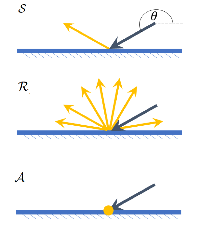
(b)

(c) Schematic of two-dimensional Poiseuille flow and individual swimmer trajectories. Swimmers are not drawn to scale.

Figure 1: Schematic of two-dimensional Poiseuille flow and individual swimmer trajectories. Swimmers are not drawn to scale. Different BC +Sample trajectories, $\beta=0.99,\nu=0.04$ with $y_{0}=0,0.6$. Dashed line is deterministic, solid has $Pe=10^{4}$. No translational peclet. Dimensionless channel

2.2 Two-dimensional channel flow

To expand upon the study of two-dimensional channel flow as motivated by experiments (rusconi2014bacterial) and numerical studies (bearon2015trapping; vennamneni2020shear), let us consider a horizontal channel of height $W$ (as shown in figure 1), such that for a coordinate system $(X,Y)$ with orthonormal base vectors $\boldsymbol{i},\boldsymbol{j}$, the channel walls are at positions $Y=\pm W/2$. Suppose there is a parabolic flow through the channel with velocity

$$\boldsymbol{u}=U\left(1-4\left(\frac{Y}{W}\right)^{2}\right)\boldsymbol{i},$$ (7)

where $U$ is the centreline flow speed of the channel.

We also take the cell orientation to be constrained in the two-dimensional place, so that the direction of orientation $\boldsymbol{p}$ can be defined in terms of the angle $\theta$ measured from the horizontal:

$$\boldsymbol{p}=\cos\theta\boldsymbol{i}+\sin\theta\boldsymbol{j}.$$ (8)

We further introduce the cell concentration distribution

$${\color[rgb]{1,0,0}\sout{n(y)=\int_{0}^{2\pi}\psi(y,\theta)d\theta.}}$$

To identify how key parameters affect the behaviour of the system, it is helpful to non-dimensionalise to reduce the number of free parameters. We have identified that two separate scalings are useful to enable the study of (I) flow effects on microswimmer distribution and (II) rotational and translational diffusion effects on swimmer and wall interactions. In scaling I (§LABEL:Sec:ScalingI), used by (bearon2015trapping), the rotational diffusion, $d_{r}$, appears in all non-dimensional parameters, and so the scaling is most useful when we can keep the rotational diffusion constant. This is appropriate when we investigate flow effects, highlight the significance of how the no-flux boundary condition is imposed, and how the boundary affects the bulk flow dynamics computed numerically in §LABEL:Sec:Nonunique. Meanwhile, with scaling II (§LABEL:Sec:ScalingII), the flow speed, $U$, appears in all non-dimensional parameters, but here we can easily examine the effects of translational and rotational diffusion (as they only appear in a single non-dimensional parameter) and study their impact on wall-interactions (§3.1, §3.2 and §3.3).

		Scaling I Scaling II
Channel width	$W$	425$\mu$m425$\mu$m
Centreline flow velocity	$U$	0mms-1–2.125mms-11.25mms-1
Swimming velocity	$V_{s}$	50$\mu$ms-150–125$\mu$ms-1
Rotational diffusion	$d_{r}$	1s-16$\times 10^{-4}$s-1–6s-1
Brownian translational diffusion	$D_{T}$	$2\times 10^{-9}\mathrm{cm}^{2}\mathrm{s}^{-1}$$2\times 10^{-9}\mathrm{cm}^{2}\mathrm{s}^{-1}$
Relative translational diffusion$d=D_{T}d_{r}/V_{s}^{2}$$10^{-4}$–Swimming Rotational Péclet number	$\epsilon=2V_{s}/Wd_{r}$ 0.2 –Rotational (Flow) Péclet number$Pe=2U/Wd_{r}$	0–101–$10^{4}$
Translational Péclet number	$Pe_{T}=WU/2D_{T}$	–1–$10^{6}$
Velocity ratio	$\nu=V_{s}/U$	–0.04-0.1

Table 1: Parameter Scaled parameter variablesfor scalings I and II, unless stated otherwise.

2.2.1 Scaling I

We nondimensionalise the system with length and time scales $L=\frac{W}{2}$ and $T_{I}=\frac{1}{d_{r}}$$T=\frac{W}{2U}$, respectively, such that our coordinate system can be redefined as $(x,y)=\left(\dfrac{2X}{W},\dfrac{2Y}{W}\right)$$(x,y)=\left(\frac{2X}{W},\frac{2Y}{W}\right)$, with boundaries located at $y=\pm 1$. This leads to Taking $\psi$ to be independent of $x$, this leads to the two-dimensional conservation equation two-dimensional conservation equation

$${\color[rgb]{1,0,0}\sout{\displaystyle{\frac{\partial\psi}{\partial t}}+\epsilon\displaystyle{\frac{\partial}{\partial y}}(\sin\theta\psi)-\epsilon^{2}d\displaystyle{\frac{\partial^{2}\psi}{\partial y^{2}}}+\displaystyle{\frac{\partial}{\partial\theta}}\left(y\mathrm{Pe}(1-\beta\cos 2\theta)\psi-\displaystyle{\frac{\partial\psi}{\partial\theta}}\right)=0}}$$

where $\epsilon=\frac{2V_{s}}{Wd_{r}}$, $d=\frac{D_{T}d_{r}}{V_{s}^{2}}$, and $Pe=\frac{2U}{Wd_{r}}$, are the swimming Péclet number, the ratio of the Brownian diffusion rate to rotational diffusion, and the rotational flow Péclet number, respectively. For this scaling, the no-flux boundary condition reduces to

$${\color[rgb]{1,0,0}\sout{\left.\int_{0}^{2\pi}\left(\sin\theta\psi-\epsilon d\displaystyle{\frac{\partial\psi}{\partial y}}\right)\mathrm{d}\theta\right|_{y=\pm 1}=0}}$$

at the boundaries. This scaling will be used in section §LABEL:Sec:Nonunique to highlight the importance of boundary conditions on the bulk flow, and why the choice of boundary conditions must be treated with care.

2.2.1 Scaling II

For scaling II, we introduce the same length scale as previously, such that the boundaries remain unchanged at $y=\pm 1$, but introduce a new time scale $T_{II}=\frac{W}{2U}$. This leads to an alternate dimensionless conservation equation

$$\displaystyle{\frac{\partial\psi}{\partial t}}+\nu\displaystyle{\frac{\partial}{\partial y}}(\sin{\theta}\,\psi)-\frac{1}{\mathrm{Pe}_{T}}\displaystyle{\frac{\partial^{2}\psi}{\partial y^{2}}}+\displaystyle{\frac{\partial}{\partial\theta}}\left(y(1-\beta\cos 2\theta)\psi-\frac{1}{\mathrm{Pe}}\displaystyle{\frac{\partial\psi}{\partial\theta}}\right)=0$$ (9)

with no-flux boundary condition

$$\left.\int^{2\pi}_{0}\left(\nu\sin\theta\psi-\frac{1}{\mathrm{Pe}_{T}}\displaystyle{\frac{\partial\psi}{\partial y}}\right)\mathrm{d}\theta\right|_{y=\pm 1}=0.$$ (10)

Here, $\nu=V_{s}/U$ $\nu=\frac{V_{s}}{U}$ is the ratio of the swimming speed to the centreline velocity, $Pe$ is the same $Pe=\frac{2U}{Wd_{r}}$ is the rotational Péclet numberas defined previously, and $Pe_{T}=WU/(2D_{T})$ , and $Pe_{T}=\frac{WU}{2D_{T}}$ is the translational Péclet number. Note here that the change in time scale focuses rotational diffusion effects to a single dimensionless quantity $Pe$, leaving the other dimensionless quantities independent of rotational diffusion.

For the steady state problem, with $psi$ independent of time, we also introduce the time-independent cell concentration distribution

$${\color[rgb]{0,0,1}\uwave{n(y)=\int_{0}^{2\pi}\psi(y,\theta)d\theta.}}$$ (11)

2.3 Cell trajectories

These conservation equations can further be transformed to an individual-based stochastic model, as there exists an established complete equivalence between forward Fokker-Planck equations and diffusion processes with a drift coefficient $\boldsymbol{\mu}(\boldsymbol{X}_{t},t)$ and diffusion coefficient $\boldsymbol{D}(\boldsymbol{X}_{t},t)$ (gardiner2009handbook). Hence, Fokker-Planck equations of the form

$${\frac{\partial\psi}{\partial t}}(\boldsymbol{x},t)=-\sum^{n}_{i=1}\displaystyle{\frac{\partial}{\partial x_{i}}}\bigg{[}\mu_{i}(\boldsymbol{x},t)\psi(\boldsymbol{x},t)\bigg{]}+\sum^{n}_{i,j=1}\displaystyle{\frac{\partial^{2}}{\partial x_{i}\partial x_{j}}}\bigg{[}D_{ij}(\boldsymbol{x},t)\psi(\boldsymbol{x},t)\bigg{]}$$ (12)

have an equivalency to Itô SDEs of the form

$$\mathrm{d}\boldsymbol{X}_{t}=\boldsymbol{\mu}(\boldsymbol{X}_{t},t)\mathrm{d}t+\boldsymbol{\sigma}(\boldsymbol{X}_{t},t)\mathrm{d}\boldsymbol{W}_{t},$$ (13)

where $\boldsymbol{X}_{t}=(y(t),\theta(t))$ is the position and orientation vector, $\mathrm{d}t$ is the time step, $\mathrm{d}\boldsymbol{W}_{t}$ is the Wiener process, $\boldsymbol{\mu}(\boldsymbol{X}_{t},t)$ is a drift term, and the diffusion effects are captured in $\boldsymbol{\sigma}(\boldsymbol{X}_{t},t)$ via the relation

$$\boldsymbol{D}(\boldsymbol{X}_{t},t)=\frac{\boldsymbol{\sigma}(\boldsymbol{X}_{t},t)\boldsymbol{\sigma}(\boldsymbol{X}_{t},t)^{T}}{2}.$$

As the two-dimensional channel flow equations are of the form of equation 12, this allows for transformation to Itô SDEs . We select scaling II for the analysis of cell trajectories, and transform equation 9 into an Itô SDE with drift and diffusion terms

$$\boldsymbol{\mu}(y,\theta,t) =\begin{pmatrix}\nu\sin\theta\\ y(1-\beta\cos 2\theta)\end{pmatrix},$$ (14a)

$$\boldsymbol{\sigma}(y,\theta,t) =\begin{pmatrix}\sqrt{\frac{2}{\mathrm{Pe}_{T}}}&0\\ 0&\sqrt{\frac{2}{\mathrm{Pe}}}\end{pmatrix}{\color[rgb]{1,0,0}\sout{,}}{\color[rgb]{0,0,1}\uwave{.}}$$ (14b)

because this formulation allows for the separation of rotational and translational diffusion effects. Taking the limits of $Pe_{T},Pe\rightarrow\infty$ we can extract the case of a purely deterministic system without diffusion. Computationally, the diffusion effects can be switched off by replacing the diagonal entries of the matrix by $0.$

For the SDE, we consider three possible boundary conditions at walls $y=\pm 1$: specular reflection, uniform random reflection and absorbing boundary. In the case of specular reflection (boundary condition $\mathcal{S}$), swimmers with angles of incidence $\theta_{i}$ instantaneously reorient to $\theta_{r}=\mathrm{mod}(2\pi-\theta_{i},2\pi)$ such that $\theta_{i},\theta_{r}\in[0,2\pi)$. For uniform random reflection (boundary condition $\mathcal{R}$)

$$\theta_{r}=\begin{cases}\pi+\pi\cdot\mathit{U}(0,1)&\quad\text{if }\theta_{i}\in[0,\pi]\text{ at }y=1,\\ \pi\cdot\mathit{U}(0,1)&\quad\text{if }\theta_{i}\in[\pi,2\pi]\text{ at }y=-1,\end{cases}$$ (15)

where $\mathit{U}(0,1)$ is a uniformly distributed random number in the interval (0,1). Meanwhile, for a perfectly absorbing boundary (boundary condition $\mathcal{A}$) trajectories terminate upon impact with a wall.

In order to visualise rotational diffusion and shape effects on downstream swimming, consider example trajectories from the IBM with boundary condition $\mathcal{S}$, as shown in figure LABEL:TrajectoriesFig, with the addition of a $x$–direction advection term such that $\boldsymbol{X}_{t}=(y(t),\theta(t),x(t))$. We neglect translational diffusion for simplicity since the focus of this paper is on the transverse distribution, and as advection in the $x$–direction would dominate translational diffusion. For this case we augment the drift and diffusion terms: In order to visualise rotational diffusion and shape effects on downstream swimming, consider example trajectories from the IBM with boundary condition $\mathcal{S}$, as shown in figure LABEL:TrajectoriesFig, with the addition of a $x$–direction advection term such that $\boldsymbol{X}_{t}=(y(t),\theta(t),x(t))$. We neglect translational diffusion for simplicity since the focus of this paper is on the transverse distribution, and as advection in the $x$–direction would dominate translational diffusion. For this case we augment the drift and diffusion terms:

$$\boldsymbol{\mu}(y,\theta,t) =\boldsymbol{\dot{X}}_{t}=\begin{pmatrix}\nu\sin\theta\\ y(1-\beta\cos 2\theta)\\ \hline\cr 1-y^{2}+\nu\cos\theta\end{pmatrix},$$ (16a)

$$\boldsymbol{\sigma}(y,\theta,t) =\left(\begin{array}[]{c c|c}\sqrt{\frac{2}{\mathrm{Pe}_{T}}}&0&0\\ 0&\sqrt{\frac{2}{\mathrm{Pe}}}&0\\ \hline\cr 0&0&0\end{array}\right).$$ (16e)

Figures LABEL:TrajectoriesFiga–LABEL:TrajectoriesFigc correspond to $Pe=10^{4}$, and $\beta=0,0.5,$ and $0.99$, respectively. Spherical swimmers in this low rotational diffusion regime are shown to swim in almost periodic trajectories, as they are advected downstream. Slightly elongated swimmers ($\beta=0.5$) have longer periods of oscillation in the $x$–direction. Highly elongated swimmers ($\beta=0.99$) traverse the furthest downstream during a single orbit as they are aligned with the flow direction for long periods of time, which is a feature of Jeffery orbits. Due to the background flow velocities being greatest about $y=0$, advection per oscillation is strongest at the channel centre, and weakest at the walls. Similar dynamics exist for $Pe=100$ (figures LABEL:TrajectoriesFigd–LABEL:TrajectoriesFigf) and $Pe=1$ (figures LABEL:TrajectoriesFigg–LABEL:TrajectoriesFigi), but increasing rotational diffusion (i.e. decreasing $Pe$) distorts the trajectories and increases the noisiness of the trajectories (comparable to purely Brownian noise).

$${\color[rgb]{1,0,0}\sout{\boldsymbol{\mu}(y,\theta,t)}} {\color[rgb]{1,0,0}\sout{=\boldsymbol{\dot{X}}_{t}=\begin{pmatrix}\nu\sin\theta\\ y(1-\beta\cos 2\theta)\\ \hline\cr 1-y^{2}+\nu\cos\theta\end{pmatrix},}}$$

$${\color[rgb]{1,0,0}\sout{\boldsymbol{\sigma}(y,\theta,t)}} {\color[rgb]{1,0,0}\sout{=\left(\begin{array}[]{c c|c}\sqrt{\frac{2}{\mathrm{Pe}_{T}}}&0&0\\ 0&\sqrt{\frac{2}{\mathrm{Pe}}}&0\\ \hline\cr 0&0&0\end{array}\right).}}$$

Figures LABEL:TrajectoriesFiga–LABEL:TrajectoriesFigc correspond to $Pe=10^{4}$, and $\beta=0,0.5,$ and $0.99$, respectively. Spherical swimmers in this low rotational diffusion regime are shown to swim in almost periodic trajectories, as they are advected downstream. Slightly elongated swimmers ($\beta=0.5$) have longer periods of oscillation in the $x$–direction. Highly elongated swimmers ($\beta=0.99$) traverse the furthest downstream during a single orbit as they are aligned with the flow direction for long periods of time, which is a feature of Jeffrey orbits. Due to the background flow velocities being greatest about $y=0$, advection per oscillation is strongest at the channel centre, and weakest at the walls. Similar dynamics exist for $Pe=100$ (figures LABEL:TrajectoriesFigd–LABEL:TrajectoriesFigf) and $Pe=1$ (figures LABEL:TrajectoriesFigg–LABEL:TrajectoriesFigi), but increasing rotational diffusion (i.e. decreasing $Pe$) distorts the trajectories and increases the noisiness of the trajectories (comparable to purely Brownian noise).

Trajectories for swimmers in $x$–$y$ plane, as obtained with scaling II, with initial positions $x_{0}=0$ and $y_{0}=-1,-0.6,0,0.6,1$ (given by the blue, red, green, purple, and yellow lines, respectively), translational Péclet number $Pe_{T}=10^{6}$, and velocity ratio $\nu=0.04$. The translational diffusivity is neglected in the $x$–direction for simplicity, and $\dot{x}=(1-y^{2})+\nu\cos\theta$, i.e. the $x$–component is comprised of swimming and advection only. Figures with $Pe=10^{4}$: (a) $\beta=0$, (b) $\beta=0.5$, and (c) $\beta=0.99$. Figures with $Pe=100$: (d) $\beta=0$, (e) $\beta=0.5$, and (f) $\beta=0.99$. Figures with $Pe=1$: (g) $\beta=0$, (h) $\beta=0.5$, and (i) $\beta=0.99$.

2.4 Numerical methods

2.4.1 SDE

To calculate the probability distribution $\psi$ from the stochastic IBM in bounded domains we run simulations for $10^{6}$ stochastic swimmers which are uniformly initialized over the domain $(\theta,y)\in[0,2\pi)\times[-1,1]$ with sampling step size $\mathrm{d}t=0.1$, and normalization condition $\int_{0}^{2\pi}\int_{-1}^{1}\psi(\theta,y)\mathrm{d}y\mathrm{d}\theta=4\pi$. The probability distribution is calculated from the end-states of all trajectories upon convergence (i.e. when doubling the run time does not change the macroscopic properties of the probability distribution).

For the bounded domains the boundary conditions are as detailed in §2.3. with details of the model and numerical method for the doubly periodic Poiseuille flow given in §3.1.1.

2.4.2 Continuum model

To solve the two-dimensional equilibrium continuum model for the probability distribution $\psi$, we a use a Galerkin finite element method, as in bearon2015trapping with the C++ library oomph-lib heil2006oomph. In §LABEL:Sec:Nonunique we We solve the problem with scaling I by simplifying equation LABEL:ScaleI 9 to the time-independent equilibrium problem, multiplying the equation by a $y$ and $\theta$ dependent test function $N(\theta,y)$, integrating over the domain, and integrating by parts, to obtain the weak solution

form

$$\int_{0}^{2\pi}\int_{-1}^{1}{\color[rgb]{1,0,0}\sout{\epsilon}}\left[{\color[rgb]{0,0,1}\uwave{\nu}}\sin\theta\psi-{\color[rgb]{1,0,0}\sout{\epsilon d}}{\color[rgb]{0,0,1}\uwave{\frac{1}{Pe_{T}}}}\displaystyle{\frac{\partial\psi}{\partial y}}\right]\displaystyle{\frac{\partial N}{\partial y}}+\left[y{\color[rgb]{1,0,0}\sout{\mathrm{Pe}}}(1-\beta\cos 2\theta)\psi-{\color[rgb]{0,0,1}\uwave{\frac{1}{Pe}}}\displaystyle{\frac{\partial\psi}{\partial\theta}}\right]\displaystyle{\frac{\partial N}{\partial\theta}}\mathrm{d}y\mathrm{d}\theta$$ (17)

$$-\int_{0}^{2\pi}{\color[rgb]{1,0,0}\sout{\epsilon}}\left[\left({\color[rgb]{0,0,1}\uwave{\nu}}\sin\theta\psi-{\color[rgb]{1,0,0}\sout{\epsilon d}}{\color[rgb]{0,0,1}\uwave{\frac{1}{Pe_{T}}}}\displaystyle{\frac{\partial\psi}{\partial y}}\right)N\right]_{-1}^{1}\mathrm{d}\theta-\int_{-1}^{1}\left[\left(y{\color[rgb]{1,0,0}\sout{\mathrm{Pe}}}(1-\beta\cos 2\theta)\psi-{\color[rgb]{0,0,1}\uwave{\frac{1}{Pe}}}\displaystyle{\frac{\partial\psi}{\partial\theta}}\right)N\right]_{0}^{2\pi}=0.$$

For the wall bounded domain, we impose the normalisation constraint $\int_{0}^{2\pi}\int_{-1}^{1}\psi(\theta,y)\mathrm{d}y\mathrm{d}\theta=4\pi$.

The equations are discretized using finite elements on a grid $n_{\theta}\times n_{y}$, where $n_{\theta}=100$ and $n_{y}=1000$, as doubling grid points has shown negligible change in distributions. with $n_{\theta}$ and $n_{y}$ varying dependent on the boundary condition type and Péclet number of interest. The elements in the $\theta$–direction are uniformly distributed and the elements in the $y$–direction are non-uniform to allow for higher resolutions near the wall. A piece-wise linear scaling is implemented to restrict half the elements to $|y|\geq 0.99$. Simple periodic boundary conditions are applied in the $\theta$–direction to ensure the angles of orientation wrap around. Similarly, the weak solution for the wall-bounded case, with scaling II, takes the form

$${\color[rgb]{1,0,0}\sout{\int_{0}^{2\pi}\int_{-1}^{1}\left[\nu\sin\theta\psi-\frac{1}{Pe_{T}}\displaystyle{\frac{\partial\psi}{\partial y}}\right]\displaystyle{\frac{\partial N}{\partial y}}+\left[y(1-\beta\cos 2\theta)\psi-\frac{1}{Pe}\displaystyle{\frac{\partial\psi}{\partial\theta}}\right]\displaystyle{\frac{\partial N}{\partial\theta}}\mathrm{d}y\mathrm{d}\theta=0}}$$

$${\color[rgb]{1,0,0}\sout{-\int_{0}^{2\pi}\left[\left(\nu\sin\theta\psi-\frac{1}{Pe_{T}}\displaystyle{\frac{\partial\psi}{\partial y}}\right)N\right]_{-1}^{1}\mathrm{d}\theta-\int_{-1}^{1}\left[\left(y(1-\beta\cos 2\theta)\psi-\frac{1}{Pe}\displaystyle{\frac{\partial\psi}{\partial\theta}}\right)N\right]_{0}^{2\pi}=0.}}$$

with the same normalisation constraint. For scaling II, the finite element problems are discretized on a grid of $n_{\theta}\times n_{y}$, with $n_{\theta}$ and $n_{y}$ varying dependent on the boundary condition type and Péclet number of interest.

In the continuum model different boundary conditions will be applied, ranging from a pointwise constraint on the flux (constraint $\mathcal{P}$)to Dirichlet constraints on $\psi$ (constraints $\mathcal{D}_{1}$ and $\mathcal{D}_{2}$), as detailed in §LABEL:Sec:Nonunique. For constraint $\mathcal{P}$ no-flux is satisfied by implementing the natural finite element boundary condition at the walls i.e. at $y=\pm 1$ the terms corresponding to vertical flux are omitted, when applying the integration by parts. . A Dirichlet constraint ($\mathcal{D}$), $\psi(\pm 1,\theta)=C_{0}$ for all $\theta$, will be imposed such that the For constraints $\mathcal{D}_{1}$ and $\mathcal{D}_{2}$ the boundary values of $\psi$ are pinned, and the values of the constants emerge upon the enforcement of the normalisation condition. Furthermore, a doubly periodic Poiseuille flow model $\mathcal{DP}$ will be detailed in §3.1.1.

3 Results

3.1 The importance of boundary conditions

To highlight the non-uniqueness of constraints thatsatisfy no-flux, let us use scaling I (§LABEL:Sec:ScalingI) when considering a wall-bounded problem. Let $J_{\theta}(y)$ be the integrand of the no-flux integral given in equation LABEL:Scale1NoFluxInt at boundary $y$ with orientation $\theta$ such that

$${\color[rgb]{1,0,0}\sout{J_{\theta}(y)=\sin\theta\psi-\epsilon d\displaystyle{\frac{\partial\psi}{\partial y}}.}}$$

We define the no-flux boundary condition as follows:

$${\color[rgb]{1,0,0}\sout{\int_{0}^{2\pi}J_{\theta}(y=\pm 1)d\theta=0.}}$$

We introduce three example boundary constraints: ($\mathcal{P}$) a pointwise boundary constraint at $y=\pm 1$ such that $J_{\theta}(y=\pm 1)=0$ for all $\theta$, ($\mathcal{D}_{1}$) a Dirichlet boundary constraint $\psi(\pm 1,\theta)=C_{0}$ for all $\theta$, and ($\mathcal{D}_{2}$) a different Dirichlet boundary constraint such that $\psi(-1,\theta)=C_{1}$, $\psi(1,\theta)=C_{2}$, and $C_{1}\neq C_{2}$ for all $\theta$. In figure LABEL:NatBCAngle we consider boundary constraint $\mathcal{P}$. For the case of a long, slender swimmer with shape parameter $\beta=0.99$, in the absence of background flows ($Pe=0$), the implementation of this boundary condition leads to a uniform cell distribution over most of the domain, except over a boundary layer near the walls. In these boundary layers, there exist large, unrealistic regions of accumulation several orders of magnitude higher than in the bulk. These artifacts arise when implementing a pointwise condition, because $\displaystyle{\frac{\partial\psi}{\partial y}}=0$ for most of the domain, but for $\sin\theta\psi=\epsilon d\displaystyle{\frac{\partial\psi}{\partial y}}$ to be satisfied for $\psi\neq 0$, where $\epsilon=0.2$ and $d=10^{-4}$ (see table 1), a sharp gradient in $y$ must develop near the boundary to match when $\sin\theta\neq 0$.

Figure highlighting the effects of boundary conditions on bulk flow and shear on the stationary probability distributionwith scaling I. Probability distributions $\psi$ for Poiseuille flow in bounded domain $\theta\times y\in[0,2\pi)\times[-1,1]$, for $\beta=0.99$, $n_{\theta}=100,n_{y}=1000$. $Pe=0$ for (a)-(c) with boundary constraints $\mathcal{P}$, $\mathcal{D}_{1}$, and $\mathcal{D}_{2}$, respectively. The emerging boundary conditions in (b) correspond to $\psi(\theta,\pm 1)=1$ and for (c) $\psi(\theta,-1)=2/3$ and $\psi(\theta,1)=4/3$. (d)&(g): Boundary condition $\mathcal{P}$ for $Pe=2$; (e)&(h): Boundary condition $\mathcal{P}$ for $Pe=6$; and (f)&(i): Boundary condition $\mathcal{P}$ for $Pe=10$.

We consider an alternative boundary constraint $\mathcal{D}_{1}$ in figure LABEL:PinnedBCAngle where we apply a Dirichlet boundary condition such that $\psi(\theta,\pm 1)=1$ for all $\theta$. The resulting uniform distribution spans the full domain, satisfying a zero distribution gradient in both $y$ and $\theta$, and the no-flux boundary integral. This is in agreement with the physically intuitive cell distribution for a suspension of swimmers in the absence of external stimuli (like chemotaxis and phototaxis), hydrodynamic wall interactions, and without the presence of background shear introducing preferred directions of orientation. But what happens when we introduce other Dirichlet boundary conditions? In figure LABEL:DiffPinnedBCAngle we impose boundary constraint $\mathcal{D}_{2}$ where the boundaries are pinned to different values, $\psi(\theta,-1)=2/3$ and $\psi(\theta,1)=4/3$. This introduces a gradient which spans the entire phase space and is no longer restricted to a thin boundary layer. This artificial gradient highlights the crucial nature of the choice of boundary conditions when modelling equilibrium systems for suspensions of swimmers via continuum methods, as these can affect the the bulk dynamics of the entire system.

While it is true that the boundary conditions can affect the bulk flow dynamics, the coupled nature of the model also leads to the bulk flow affecting boundary distributions. In figures LABEL:NatBCPe2–LABEL:NatBCPe10ii we introduce linearly varying background shear flows with pointwise boundary conditions (constraint $\mathcal{P}$), with $Pe=2$ in figures LABEL:NatBCPe2, LABEL:NatBCPe2ii; $Pe=6$ in figures LABEL:NatBCPe6, LABEL:NatBCPe6ii; and $Pe=10$ in figures LABEL:NatBCPe10, LABEL:NatBCPe10ii. The introduction of a background flow leads to regions of cell accumulation and depletion (which will be discussed in more detail in §3.2) in most of the bulk. However, near the wall, the behaviour deviates from the observed accumulation region distributions and a boundary layer develops. In the boundary layers, there are large peaks of accumulation, allowing us to quantify the boundary layer by three features: the height of the peaks (level of cell accumulation), the span (width) of the peaks in orientation space, and the thickness of the boundary layers in $y$–space. The height of the peaks decrease monotonically with increase in flow rate (reflected here by an increase in $Pe$), from $\mathcal{O}(10^{4})$ in figure LABEL:NatBCAngle ($Pe=0$) to $\mathcal{O}(10^{3})$ in figures LABEL:NatBCPe10,LABEL:NatBCPe10ii ($Pe=10$). Meanwhile, the orientation width of the peaks at half the peak-heights $w(\psi_{peak}/2,Pe)$ decreases with increased $Pe$, as $w(\psi_{peak}/2,0)=1.7$, $w(\psi_{peak}/2,2)=0.94$, $w(\psi_{peak}/2,6)=0.57$, and $w(\psi_{peak}/2,10)=0.5$. Finally, we find that increases in background flow lead to a decrease in boundary layers thickness (in $y$–space) as the bulk flow dynamics dominate boundary effects. By defining the boundary layer thickness as the layer over which there is a 10% deviation in cell concentration $n(y)$ we find the boundary layer thicknesses to be $BL(Pe=2)=0.04$, $BL(Pe=6)=0.035$, and $BL(Pe=10)=0.015$.

While it is easy to discern that the constant boundary conditions in figure LABEL:PinnedBCAngle are reasonable conditions for the case of no shear, the matter of discerning sensible continuum boundary conditions for sheared flows is less obvious. In the next sections we will determine a systematic, sensible approach to selecting continuum boundary conditions for sheared flows, and study the contributions of diffusion effects. For clarity, and to allow for the study of diffusion effects, we will only use systems with scaling II from here on.

3.1 What is a sensible no-flux boundary condition for the continuum model?

Figure 2: A comparison of the bulk dynamics in a continuum double-Poiseuille model, to a stochastic bounded simulation with wall-bounded specular reflection with scaling II, for $Pe=10$, $\beta=0.99$, $\nu=0.04,$ and $Pe_{T}=10^{6}$. (a) Finite element continuum simulation for ($n_{\theta}=100,n_{y}=500$) double-Poiseuille bivariate $\psi$ distribution for flow with periodic boundaries; (b) IBM stochastic bivariate $\psi$ distribution for single Poiseuille flow with point-wise no-flux conditions at $y=\pm 1$; (a)–(c): Example trajectories of cells swimming in sheared flow in $\theta$-$y$ phase space (white lines), with snapshots in time given by dots along each trajectory (black to white in time). Cell trajectories are overlaid over bivariate probability distribution $\psi$, as obtained from IBMs with specular reflection boundary conditions (condition $\mathcal{S}$) for $\beta=0.99$ and $\nu=0.04$. (a): IBM with $Pe=10$ and $Pe_{T}=10^{3}$;(c) Flow profile for double-Poiseuille flow in (a).

As highlighted in figure LABEL:Fig1, As there is no unique formulation for implementing an integral no-flux boundary condition, and it is necessary to carefully select additional boundary constraints. We will consider an IBM with specular reflection (IBM condition $\mathcal{S}$) and examine what continuum approaches/boundary conditions best fit it. In particular we will investigate the approach of using a double periodic Poiseuille flow $\mathcal{DP}$. In the literature, double-Poiseuille flows have been used for studying low and high shear trapping of bacterial suspensions to circumvent the problem of explicitly implementing a boundary (vennamneni2020shear). Further IBM boundary conditions such as uniform random reflection (condition $\mathcal{R}$) and perfectly absorbing boundaries (condition $\mathcal{A}$) will be explored in the next section (§3.2).

3.1.1 Doubly periodic Poiseuille flow

As the doubly periodic Poiseuille flow serves as a potential alternative for capturing the bulk flow in the bounded domain, we adapt the finite element model with a doubly periodic flow profile as shown in figure 2c. For this, the background fluid flow, $\boldsymbol{u}$, for domain $y\in[-3,1]$, becomes

$$\boldsymbol{u}=\begin{cases}(1-y^{2}){\boldsymbol{i}}&\textrm{ for }y>-1\\ -(1-(y+2)^{2}){\boldsymbol{i}}&\textrm{ for }y<-1\\ \end{cases}$$ (18)

such that the background flow for $y\in[-1,1]$ is identical to the background flow for a simple Poiseuille flow in the channelas derived with scaling II. . For this extended domain we implement periodic boundary conditions $\mathcal{DP}$

$$\psi(\theta,-3) =\psi(\theta,1),$$ (19a)

$$\psi(0,y) =\psi(2\pi,y),$$ (19b)

and normalisation condition $\int_{0}^{2\pi}\int_{-2}^{2}\psi(\theta,y)\mathrm{d}y\mathrm{d}\theta=8\pi$. The double-Poiseuille flow profile is $\mathcal{C}^{0}$ continuous in shear and $\mathcal{C}^{1}$ continuous in velocity at $y=\pm 1$. While the introduction of the doubly periodic Poiseuille flow velocity profile introduces a discontinuity in the second derivative of the flow velocity in $y$ about $y=-1$, this does not lead to any difficulties with the finite element discretisation, as the implementation only requires continuity of the first derivative.

(a)–(c): Example trajectories of cells swimming in sheared flow in $\theta$-$y$ phase space (white lines), with snapshots in time given by dots along each trajectory (black to white in time). Cell trajectories are overlaid over bivariate probability distribution $\psi$, as obtained from IBMs with specular reflection boundary conditions (condition $\mathcal{S}$) for $\beta=0.99$ and $\nu=0.04$. (a): IBM with $Pe=10$ and $Pe_{T}=10^{3}$; (b): IBM with only rotational diffusion effects $Pe=10$; (c): Fully deterministic IBM without diffusion effects. The red line separates between different modes of swimming and the yellow line separates between swimmers which interact with the bottom wall in the absence of diffusion and those which do not; (d) Divergence of macroscopic deterministic drift effects, $\chi=-div(\boldsymbol{\mu})$, highlighting regions of expected inwards ($\chi>0$) and outward cell flux ($\chi<0$), i.e. expected regions of accumulation and depletion, respectively.

Comparing the subdomain for the finite element double-Poiseuille model $\theta\in[0,2\pi],y\in[-1,1]$ in figure 2a to the bounded, stochastic IBM with boundary condition $\mathcal{S}$ in figure 2b, for $Pe=10$, $Pe_{T}=10^{6}$, $\nu=0.04$ and $\beta=0.99$, we find similar bulk-flow dynamics with regions of cell accumulation above $y=-1$, at angles slightly greater than $\theta=0,\pi$. Meanwhile, just below $y=1$, near the ‘upper wall,’ there also exist two areas of accumulation of equal intensity, but of flipped geometry, for angles just below $\theta=2\pi$ and $\theta=\pi$. In both cases, these areas of accumulation correspond to swimmers oriented close to the horizontal, but pointing into the wall and out of the wall, respectively.

Stacked probability distribution of angle of incidence for particles striking the lower wall ($y=-1$), for $\nu=0.04$ and $Pe_{T}=10^{6}$. The blue distribution corresponds to particles which are expected to strike the wall in the absence of diffusive effects (originating in region 1), and the red, correspond to particles that would not strike the bottom wall in the absence of diffusive effects (originating in region 2). The overall envelope characterises the distribution of cells striking the bottom wall and integrates to 1. For $\beta=0.99$, (a)$Pe=10^{4}$, (b)$Pe=100$, and (c)$Pe=1$. (d) Ratio of cell–wall interactions with cells originating in region 1 to total cell–wall interactions, for varying $\beta$ and Péclet numbers.

While this qualitatively suggests consistency in the bulk flow dynamics observed via the double-Poiseuille continuum model with the bounded stochastic IBM model, further study is required to determine if the equilibrium distributions obtained from the double-Poiseuille models at $y=\pm 1$ compare closely with the observed bounded Stochastic IBM Eulerian solutions captured with specular reflective boundaries $\mathcal{S}$. Before examining in detail the comparison between the two models (figures 3 and 4), we first consider the effects of diffusion on the system (figures LABEL:Fig3 and 8).

In figure LABEL:Fig3 we highlight the roles of translational and rotational diffusion on the equilibrium distribution, and the origin of the macroscopic regions of accumulation and depletion. In all figures, individual trajectories in time (white lines)are highlighted via dots witha gradient from black to white. We begin by considering the full IBM problem in figure LABEL:Fig3a, with diffusion effects quantified by $Pe=10$ (rotational diffusion) and $Pe_{T}=1000$ (translational diffusion). The lowest trajectory in figure 2 highlights a cell trajectory which enters a region of accumulation close to the bottom wall, while oriented parallel to the flow direction ($\theta=\pi)$. The cell moves up and down the channel height, while approximately maintaining its orientation parallel to the flow direction due to translational diffusion effects. Meanwhile, in the presence of only rotational diffusion (figure LABEL:Fig3b), there is little $y$–variation in the lowest trajectory, but there is some orientational variation with the clumping and widening of cell positionsmeasured at equal time separations, due to rotational diffusion counteracting and enhancing reorientations due to Jeffery orbits, respectively. The removal of translational diffusion effects also allows for slightly sharper regions of accumulation than in figure 2, as seen by slightly larger values of $\psi$ in the areas of accumulation. In figure LABEL:Fig3c, we consider the fully deterministic case, where no rotational or translational diffusion affects the swimmer. Any cell which enters the region of accumulation will exit it along predetermined pathlines, and only after the completion of a full orbit can a cell revisit the region of accumulation. The accumulation measured in that case is solely by virtue of cells spending longer periods aligned with the flow direction as described by Jeffery orbits. In figure LABEL:Fig3 we highlight the roles of translational and rotational diffusion on the equilibrium distribution, and the origin of the macroscopic regions of accumulation and depletion. In all figures, individual trajectories in time (white lines) are highlighted via dots with a gradient from black to white. We begin by considering the full IBM problem in figure LABEL:Fig3a, with diffusion effects quantified by $Pe=10$ (rotational diffusion) and $Pe_{T}=1000$ (translational diffusion). The lowest trajectory in figure 2 highlights a cell trajectory which enters a region of accumulation close to the bottom wall, while oriented parallel to the flow direction ($\theta=\pi)$. The cell moves up and down the channel height, while approximately maintaining its orientation parallel to the flow direction due to translational diffusion effects. Meanwhile, in the presence of only rotational diffusion (figure LABEL:Fig3b), there is little $y$–variation in the lowest trajectory. However, there is some orientational variation with the clumping and widening of cell positions measured at equal time separations. This results from rotational diffusion counteracting and enhancing reorientations due to Jeffery orbits, respectively. The removal of translational diffusion effects also allows for slightly sharper regions of accumulation than in figure 2, as seen by slightly larger values of $\psi$ in the areas of accumulation. In figure LABEL:Fig3c, we consider the fully deterministic case, where no rotational or translational diffusion affects the swimmer. Any cell which enters the region of accumulation will exit it along predetermined pathlines, and only after the completion of a full orbit can a cell revisit the region of accumulation. The accumulation measured in that case is solely by virtue of cells spending longer periods aligned with the flow direction as described by Jeffery orbits.

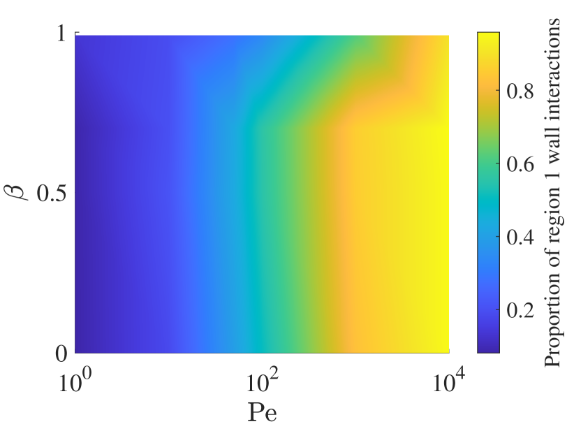
(d)

(e)

Figure 8: Stacked probability distribution of angle of incidence for particles striking the lower wall ($y=-1$), for $\nu=0.04$ and $Pe_{T}=10^{6}$. The blue distribution corresponds to particles which are expected to strike the wall in the absence of diffusive effects (originating in region 1), and the red, correspond to particles that would not strike the bottom wall in the absence of diffusive effects (originating in region 2). The overall envelope characterises the distribution of cells striking the bottom wall and integrates to 1. For $\beta=0.99$, (a)$Pe=10^{4}$, (b)$Pe=100$, and (c)$Pe=1$. (d) Ratio of cell–wall interactions with cells originating in region 1 to total cell–wall interactions, for varying $\beta$ and Péclet numbers. (e): Fully deterministic IBM without diffusion effects. The red line separates between different modes of swimming and the yellow line separates between swimmers which interact with the bottom wall in the absence of diffusion and those which do not.

In figure 2, the macroscopic areas of accumulation are dependent on both the shape and the motility of the swimmers. The fluid itself is incompressible and cannot by itself cause the stratification between regions of accumulation and depletion. Taking the negative divergence of the deterministic dynamics (the drift component of the SDE with $\boldsymbol{\mu}$ defined in §2.3), $\chi=-\boldsymbol{\nabla}_{y,\theta}\cdot\boldsymbol{\mu}=-2\beta y\sin 2\theta$, we can quantify a measure of the inward flux at any point in the phase space as shown in figure LABEL:MinusDivergence. The regions of outward flux and inward flux, given in blue and yellow, respectively, roughly correspond to the areas of depletion and accumulation found from the individual and continuum models. In reality the drift related fluxes are balanced by diffusion. The thickness and position of the areas of accumulation are also dependent on the diffusion effects. In figure LABEL:IBMwithoutDT, we find that in the absence of translational diffusion, the width of the peaks decreases. Meanwhile, in the absence of all diffusion (figure 8(e)), there are only thin areas of accumulation about $\theta=0,\pi$ which correspond to the cusps of the deterministic trajectories. In this case, maximal accumulation occur at $\theta=\pi$ just within the cusp of the red separatrix which separates cell between those which completely $2\pi$ rotations per trajectories and those which only wobble in orientation (see rusconi2014bacterial).We can further separate the regions with trajectories that will interact with the lower wall, and those that will not, by the yellow line. We call the area of guaranteed interactions (below the yellow line) ‘Region 1’, and the area above ‘Region 2’. In the absence of diffusion, all cell trajectories are predetermined, and only Region 1 cells interact with the walls. However, with increasing diffusion, larger quantities of microswimmers cross the streamlines, and more cells from Region 2 interact with the walls. The shift in interactions is captured in figure 8 for fixed IBM runtime $T_{sim}=600$ through stacked probability distributions, where the total number of wall interactions across 51 bins are normalised to 1. For the case of $Pe=10^{4}$ with $\beta=0.99$, the orientation distribution peaks tend toward $\theta\rightarrow\pi$ as $\beta\rightarrow 1$. In this low rotational diffusion case, over80% of all wall interaction originate from region 1, and this percentage decreasesmonotonically with $Pe$, irrespective of swimmer shape (see figures 8a,d). An increase in rotational diffusivity, corresponding to $Pe=1$ (figure 8c) shifts the peak of the distribution $\theta_{peak}\rightarrow 3\pi/2$, and the size of the peak decreases with a decrease in $\beta$ (see figure 13). In figure 2b, the macroscopic areas of accumulation are dependent on both the shape and the motility of the swimmers. The fluid itself is incompressible and cannot by itself cause the stratification between regions of accumulation and depletion. Taking the negative divergence of the deterministic dynamics (the drift component of the SDE with $\boldsymbol{\mu}$ defined in §2.3), $\chi=-\boldsymbol{\nabla}_{y,\theta}\cdot\boldsymbol{\mu}=-2\beta y\sin 2\theta$, we can quantify a measure of the inward flux at any point in the phase space as shown in figure LABEL:MinusDivergence. The regions of outward flux and inward flux, given in blue and yellow, respectively, roughly correspond to the areas of depletion and accumulation found from the individual and continuum models. In reality the drift related fluxes are balanced by diffusion. The thickness and position of the areas of accumulation are also dependent on the diffusion effects. In figure LABEL:IBMwithoutDT, we find that in the absence of translational diffusion, the width of the peaks decreases. Meanwhile, in the absence of all diffusion (figure 8(e)), there are only thin areas of accumulation about $\theta=0,\pi$ which correspond to the cusps of the deterministic trajectories. In this case, maximal accumulation occur at $\theta=\pi$ just within the cusp of the red separatrix which separates cell between those which complete $2\pi$ rotations per trajectories and those which only wobble in orientation (see rusconi2014bacterial). We can further separate the regions with trajectories that will interact with the lower wall, and those that will not, by the yellow line. We call the area of guaranteed interactions (below the yellow line) ‘Region 1’, and the area above ‘Region 2’. In the absence of diffusion, all cell trajectories are predetermined, and only Region 1 cells interact with the walls. However, with increasing diffusion, larger quantities of microswimmers cross the streamlines, and more cells from Region 2 interact with the walls. The shift in interactions is captured in figure 8 for fixed IBM runtime $T_{sim}=600$ through stacked probability distributions, where the total number of wall interactions across 51 bins are normalised to 1. For the case of $Pe=10^{4}$ with $\beta=0.99$, the orientation distribution peaks tend toward $\theta\rightarrow\pi$ as $\beta\rightarrow 1$. In this low rotational diffusion case, over 80% of all wall interaction originate from region 1, and this percentage decreases monotonically with $Pe$, irrespective of swimmer shape (see figures 8a,d). An increase in rotational diffusivity, corresponding to $Pe=1$ (figure 8c) shifts the peak of the distribution $\theta_{peak}\rightarrow 3\pi/2$, and the size of the peak decreases with a decrease in $\beta$ (see figure 13).

Next, we consider the comparative distributions obtained from the doubly periodic IBM (figure 3a), the doubly periodic continuum model (figure 3b), and the wall-bounded IBM with specular reflection $\mathcal{S}$ (figure 3c). We compare the cell concentration distributions of swimmers, $n(y)$, across the channel height $y\in[-1,1]$ for $\beta=0.99$, for different values of rotational diffusion ($Pe=1,10,100,10^{4}$). Direct comparison of the three models for $\beta=0.99$ show clear agreement in the cell concentrations and accumulations, except some depletion of the cell concentration at the walls for the specular reflection IBM. The observed depletion is a numerical artifact of specular reflection in the IBM, in which the finite time step causes cell trajectory overshoots, leading to some cell depletion about $\theta=0$ for $y=-1$ and $\theta=\pi$ at $y=1$, as seen in figure 2 (see Appendix A for details). We note that the depletion of cells is most pronounced for intermediate values of $Pe$. For high $Pe$ the migration of cells towards the channel centre due to low shear trapping (vennamneni2020shear) results in low cell concentrations at the wall, therefore minimising the effect that overshooting may have on the cell distribution concentration. Meanwhile, for low $Pe$, the high rotational diffusion results in any artificial depletion being largely counteracted, thereby reducing the dip in cell concentrations. Finally, for intermediate values of $Pe$ high shear trapping ensures a high enough concentration of cells near the walls for a dip to be noticeable, and the rotational diffusion effects are not sufficiently large to counteract the cell depletion due to overshooting. Nevertheless, the observed structures and positions of cell distributions obtained across all three models are in good agreements across the studied range of rotational diffusions, with clear centreline cell depletion measured for medium to high rotational effects (low to medium Péclet numbers) which are observed in experiments (rusconi2014bacterial) as well as numerical and analytical studies (bearon2015trapping; vennamneni2020shear). Meanwhile, in the limiting case of low diffusive effects ($Pe=10^{4}$) tending towards a purely deterministic case, cells are mostly trapped in fixed trajectories with peaks in cell accumulation at the cusps of the separatrices between continuously rotating and oscillating trajectories as highlighted in red in figure 8(e) and predicted by rusconi2014bacterial and zottl2013periodic. The strong agreement in the bulk flow and near the walls suggests that the doubly periodic Poiseuille continuum model might be a sensible modification for capturing the cell distributions of swimmers undergoing specular reflection at the walls.

Next, we consider the comparative distributions obtained from the doubly periodic IBM (figure 3a), the doubly periodic continuum model (figure 3b), and the wall-bounded IBM with specular reflection $\mathcal{S}$ (figure 3c). We compare the cell concentration distributions of swimmers, $n(y)$, across the channel height $y\in[-1,1]$ for $\beta=0.99$,for different values of rotational diffusion ($Pe=1,10,100,10^{4}$). Direct comparison of the three models for $\beta=0.99$ show clear agreement in the cell concentrations and accumulations, except some depletion of the cell concentration at the walls for the specular reflection IBM. The observed depletion is a numerical artifact of specular reflection in the IBM, in which the finite time step causes cell trajectory overshoots, leading to some cell depletion about $\theta=0$ for $y=-1$ and $\theta=\pi$ at $y=1$, as seen in figures 2 and LABEL:IBMwithoutDT (see Appendix A for details). We note that the depletion of cells is most pronounced for intermediate values of $Pe$. For high $Pe$ the migration of cells towards the channel centre due to low shear trapping (vennamneni2020shear) results in low cell concentrations at the wall, therefore minimising the effect that overshooting may have on the cell distribution concentration. Meanwhile, for low $Pe$, the high rotational diffusion results in any artificial depletion being largely counteracted, thereby reducing the dip in cell concentrations. Finally, for intermediate values of $Pe$ high shear trapping ensures a high enough concentration of cells near the walls for a dip to be noticeable, and the rotational diffusion effects are not sufficiently large to counteract the cell depletion due to overshooting.Nevertheless, the observed structures and positions of cell distributions obtained across all three models are in good agreements across the studied range of rotational diffusions, with clear centreline cell depletion measured for medium to high rotational effects (low to medium Péclet numbers) which are observed in experiments (rusconi2014bacterial) as well as numerical and analytical studies (bearon2015trapping; vennamneni2020shear). Meanwhile, in the limiting case of low diffusive effects ($Pe=10^{4}$) tending towards a purely deterministic case, cells are mostly trapped in fixed trajectories with peaks in cell accumulation at the cusps of the separatrices between continuously rotating and oscillating trajectories as highlighted in red in figure 8(e) and predicted by rusconi2014bacterial and zottl2013periodic. The strong agreement in the bulk flow and near the walls suggests that the doubly periodic Poiseuille continuum model might be a sensible modification for capturing the cell distributions of swimmers undergoing specular reflection at the walls.

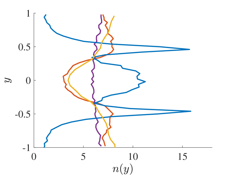
(a)

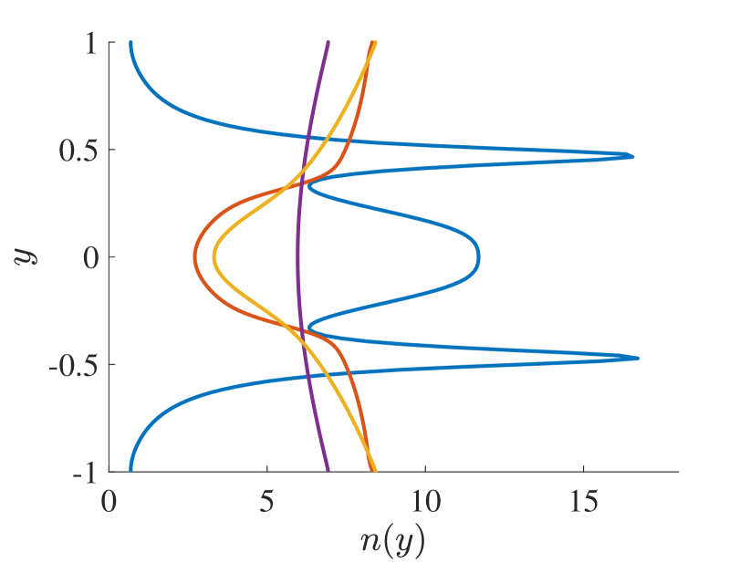
(b)

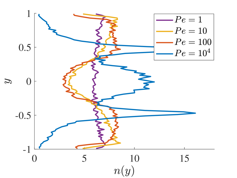
(c)

Figure 3: Cell number density distributions for (a): IBM with doubly periodic Poiseuille flow; (b): the distribution of continuum modelling with doubly periodic Poiseuille; and (c): the IBM distribution with a wall bounded boundary condition. For shape parameters $\beta=0.99$ with $Pe=10^{4}$ (blue), $Pe=100$ (red), $Pe=10$ (yellow) and $Pe=1$ (purple).

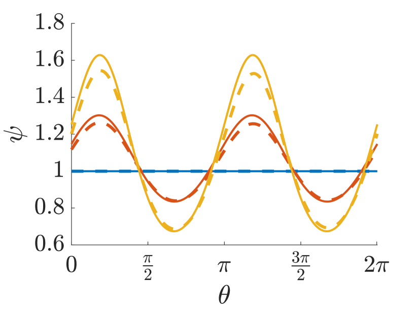
(a)

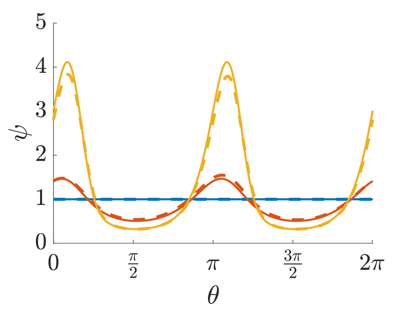
(b)

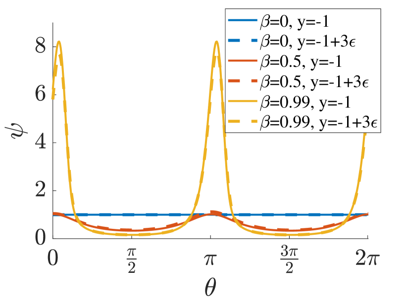
(c)

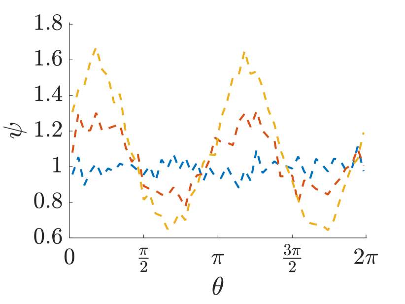
(d)

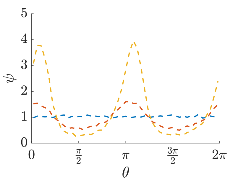
(e)

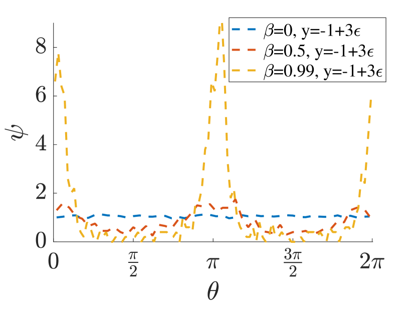
(f)

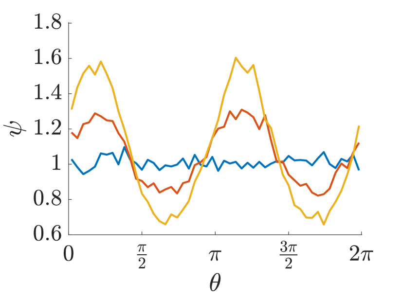
(g)

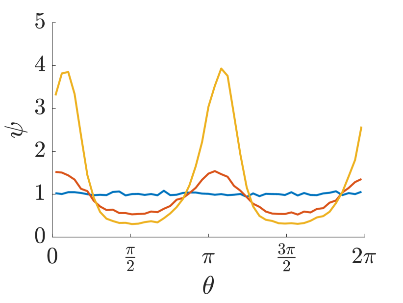
(h)

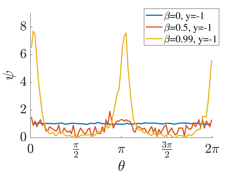
(i)

Figure 4: Comparing the distributions at the wall for varying $Pe$ and $\beta$, between the doubly periodic continuum model and the wall-bounded specular reflection IBM for $\nu=0.04$ and $\beta=0,0.5,0.99$. The probability distributions $\psi$ at $y=-1$ (solid lines) and $y=-1+3\epsilon$ (dashed lines) for the double-Poiseuille continuum model, for (a) $Pe=1$ ($n_{\theta}=100$, $n_{y}=500$); (b) $Pe=10$ ($n_{\theta}=200$, $n_{y}=500$); and (c) $Pe=100$ ($n_{\theta}=400$, $n_{y}=200$). The probability distributions $\psi$ near the bottom wall $y=-1+3\epsilon$ for the wall-bounded IBM with specular reflection, for (d) $Pe=1$; (e) $Pe=10$; and (f) $Pe=100$. The probability distributions $\psi$ at the centreline at $y=-1$ for the doubly periodic Poiseuille IBM, for (g) $Pe=1$; (h) $Pe=10$; and (i) $Pe=100$.

While the cell concentration distribution $n(y)$ tells us about the agreement in the relationship between the three models in terms of cell accumulation, it does not allow for any insight into the orientations of the swimmers at or near the walls. In figure 4 we compare the probability density distributions $\psi(\theta,y)$ for the doubly periodic Poiseuille flow continuum model (figures 4(a)–4(c)), the IBM specular reflection model (figures 4(d)–4(f)), and the IBM double periodic Poiseuille flow case (figures 4(g)–4(i)), for Péclet numbers $Pe=1$ (figures 4a, 4d, 4g), $Pe=10$ (figures 4b, 4e, 4h), and $Pe=100$ (figures 4c, 4f, 4i). For direct comparison between the doubly Poiseuille models we plot the distributions at $y=-1$, given by solid lines, for shape parameter $\beta=0,0.5,0.99$. To provide a comparison between the continuum model and the IBM we need to account for the numerical cell depletion due to numerical overshooting for long run-times. To capture near-wall cell distributions at $T=600,$ we plot the probability distributions near the walls just beyond the numerically artificial depletion area at $y=-1+3\epsilon$ for $\epsilon=0.04$, as dashed lines.

We note that across the continuum models for spherical swimmers ($\beta=0$ given by the blue lines), the orientation distribution is constant, indicating that surface interactions in the absence of hydrodynamic wall interactions, show no preferential orientation. This uniformity is due to spherical swimmers undergoing a constant rate of reorientation in sheared flows as spheres have no preferred direction. This is confirmed further by both IBM models, which despite noisiness, do not display any preferential wall interactions orientations for all considered orientational Péclet numbers.

For the case of high rotational diffusion, $Pe=1$, we note that all distributions for non-spherical swimmers peak at approximately $\theta=\pi/4$ and $\theta=5\pi/4$ (with troughs at approximately $\theta=3\pi/4$ and $\theta=7\pi/4$) across all models, with peak concentrations increasing with cell elongation. As the rotational diffusion decreases, corresponding to an increase in the rotational Péclet number, the peaks shift towards $\theta=0$ and $\theta=\pi$ for all $\beta$, with peaks clearly sharpening for the case of $\beta=0.99$.

While the peaks for $\beta=0.5$ were $\psi_{peak}\approx 1.3$ at $Pe=1$, for $Pe=10$ this rises to $\psi_{peak}\approx 1.5$, and for $Pe=100$ decreases to $\psi_{peak}\approx 1$. The shift in peaks has a two-fold origin: the relative roles of deterministic versus diffusion effects, and the shift in the bulk cell distributions due to high- and low-shear trapping. In the former case, as rotational diffusion effects decrease (increase from $Pe=1$ to $Pe=10$) the decrease in randomness leads to decreased orientational spreading and sharper peaks. The slight elongation of cells ($\beta=0.5$) also results in cells spending more time aligned parallel to the flow direction. Meanwhile high- and low-shear trapping are phenomena observed by vennamneni2020shear, where high-shear trapping refers to the shape and rotational diffusion dependent migration of cells towards channel walls and similarly low-shear trapping refers to the migration of swimmers towards the centreline. In our studies, both high-shear trapping and low-shear trapping are captured for $\beta=0.99$, as evidenced by the high-shear trapping leading the peak of the wall distribution increasing from $\psi_{peak}\approx 1.6$ to $\psi_{peak}\approx 4$ to $\psi_{peak}\approx 8$, for $Pe=1,10,100$, respectively, before a transition to low-shear trapping for $Pe=10^{4}$ in figure 3 as the cells move away from the walls.

We further compare the profiles across the different models. For a small Péclet number $Pe=1$ (see figures 4(a) and 4(d)) the profiles at $y_{near}$ (the dashed lines) are in good agreement, with similar peak magnitudes and spreads. Although the IBM distributions for $\beta=0$ are noisy about $\psi_{peak}=1$ for all Péclet values, they are in agreement with the doubly Poiseuille cases in figures 4(a)–4(f). For $Pe=100$ and $\beta=0.99$ (figures 4(c) and 4(f)) for the case of $\beta=0.99$, while the the central peaks about $\theta=\pi$ are of similar height, the central peak . However, the central peak about $\theta=0$ is slightly larger in the individual based model, as the overshooting of particles from bounded trajectories is depleting the peak profile about $\theta=0$. The depletion of the peak is, however, minor as the rotational diffusion is sufficiently large to feed more cells into the depletion areas. It is further worth noting that at $Pe=100$ overshooting in long time distributions is only significant at $y_{near}$ for elongated swimmers as the deterministic trajectories of elongated swimmers point more sharply away from the wall about $\theta=0$, leading to an increased radius of depletion compared to more spherical swimmers.

We further seek to confirm that the discrepancy between the models is due to cell leaking leading to depletion, and that the IBM system can effectively capture dynamic equilibria found via our continuum model, we run further double-Poiseuille simulations, this time for the IBM in figures 4g–4i, corresponding to $Pe=1,10,100$. After allowing for sufficiently long runtimes, we find that the probability distributions at $y=-1$ (solid lines) match with those obtained from the continuum model 4a–4c.

Comparing across all models, we find a remarkably good fit in the probability distributions within the studied range of rotational diffusion strengths and elongations. We see that all peak height and width distributions are in agreement across the three models, with only a slight discrepancy between the peak heights at $Pe=100$ for $\beta=0.99$ in the specular reflection IBM due to the aforementioned overshooting, indicating the onset of the limitations of the stochastic specular reflection IBM occurs at high $Pe$ and strong elongation.

The good fit between the specular reflection IBM and the doubly periodic Poiseuille continuum model raises the question of how the doubly periodic model’s symmetry constraints on $\psi$ and $\displaystyle{\frac{\partial\psi}{\partial y}}$ at $y=\pm 1$ compare to the literature (jiang2019dispersion; jiang2020dispersion). From figure 4, we note that at the walls, the cell probability density distributions satisfy $\psi(\theta,\pm 1)=\psi(\theta+\pi,\pm 1)$. With the periodic boundary, the derivative satisfies $\displaystyle{\frac{\partial\psi}{\partial y}}(\theta,\pm 1)=-\displaystyle{\frac{\partial\psi}{\partial y}}(\theta+\pi,\pm 1)$. The combination of these symmetries ensure that the flux condition $J_{\theta}(\pm 1)=-J_{\theta+\pi}(\pm 1)$ and the integral no-flux boundary condition and impermeability are satisfied for the equilibrium problem. We note that this observed boundary flux relationship differs from jiang2019dispersion; jiang2021transient, in which for their time evolving continuum models with non-uniform initial condition, the flux condition itself was prescribed to be specular, by imposing the equivalent of $J_{\theta}(\pm 1)=-J_{2\pi-\theta}(\pm 1)$, through the constraints $\psi(\theta,\pm 1)=\psi(2\pi-\theta,\pm 1)$ and $\displaystyle{\frac{\partial\psi}{\partial y}}(\theta,\pm 1)=-\displaystyle{\frac{\partial\psi}{\partial y}}(2\pi-\theta,\pm 1)$, in our coordinate system. We note that their imposed conditions satisfy the no-flux condition, and though the bulk results are consistent across their and our models, we do not find agreement between their imposed wall behaviours and those that emerge in our equilibrium studies. We find from our IBMs that imposing specular reflection in instantaneous wall interactions does not result in a long-term distribution in the equilibrium solution which satisfies $\psi(\theta,\pm 1)=\psi(2\pi-\theta,\pm 1)$. Therefore, the boundary conditions used by jiang2019dispersion; jiang2021transient are not consistent with the distribution that naturally emerges from our IBM with specular reflection and that also emerges as the ‘boundary solution’ in the doubly Poiseuille periodic continuum model.

3.2 Further boundary conditions

While we have shown that the dynamics from specular reflection are well captured by a continuum approximation with doubly periodic boundary conditions, we know that microswimmers’ surface interactions are not perfect specular reflections. A swimmer near the wall may remain oriented upstream for a significant period of time, it may attach to the surface, or it may leave the surface at varying outgoing angles which may be independent of the incident angles. Keeping this in mind, we consider the effects of two further wall-interaction models: perfectly random reflections (§3.2.1) and perfect absorption (§3.2.2)

3.2.1 Random reflections (boundary condition $\mathcal{R}$)

In this section we consider the effects of random uniform reflections at the boundaries on the equilibrium dynamics of microswimmer suspensions. Suppose we have a random uniform reflection out of the wall for each incident swimmer, independent of the angle of incidence, as described by equation 15. In figures 5(a)–5(c), we see the bivariate cell probability density distribution $\psi$ for $\beta=0.99$ for varying rotational Péclet numbers. By inspection, the bulk flow distributions are similar to those found via the doubly periodic continuum model and the specular reflection IBM, with areas of cell accumulations which sharpen with increased $Pe$. However, from figure 5(c) we clearly note the appearance of secondary peaks at $y=\pm 0.93$ for $Pe=10^{4}$, and also note a smaller peak for $Pe=100$ (figure 5(b)). No clear peak is visible for $Pe=1,$ as rotational effects dominate the deterministic secondary structures. We note further, that the upper bound of the aforementioned secondary peaks are bounded at $\theta=0$ by the cusp of the deterministic trajectory originating from $y=-1$ and $\theta=\pi$ (the yellow separatrix from figure 8(e)).

Noting that the secondary peaks are wholly introduced by the uniform reflective conditions, we seek to determine the appropriate continuum model boundary condition to obtain the corresponding bulk dynamics. To capture the uniformity of reflection, and lack of orientation preference upon reflection, we consider a continuum model with a constant Dirichlet wall-boundary condition (constraint $\mathcal{D}_{1}$ $\mathcal{D}$ introduced in §LABEL:Sec:Nonunique2.4.2) such that $\psi$ is the same constant on both walls and the value of this constant emerges when enforcing the normalising condition. From figures 5(d)–5(f) we find that the same secondary peaks, indicating that slightly away from the wall there is an enhanced number of cells swimming downstream.

To further confirm the suitability of comparing the IBM with random uniform reflection to the continuum model with a constant Dirichlet boundary condition, we consider the cell number density distributions in figure 6. Comparing figures 6(a) and 6(b) for $\beta=0.99$, we find that both profiles for $Pe=10^{4}$ (the blue lines) have the same primary peaks about $y=\pm 0.5$ as observed for the IBM with specular reflection, but we also get a significant peak in density about $y=\pm 0.93$ in both figures. While there are discrepancies in the size of the secondary peaks found via the IBM, we note that their size is limited by the finite time steps. Too large time steps result in cells overshooting and depleting away from the secondary peaks. We find that there is a computational trade off in the total runtime required to capture the macroscopic effects (such as the peaks and troughs) and the smallness of timesteps required to capture the slim secondary peaks. We further note that in both the continuum and IBM models the minimum cell densities occur at $y\approx\pm 0.85$. We similarly find the distributions for $Pe=100$ to be a good match with the previous models (figure 3) except at the locations of the secondary peaks. Meanwhile, for $Pe=1$, there is no significant secondary peak as expected.

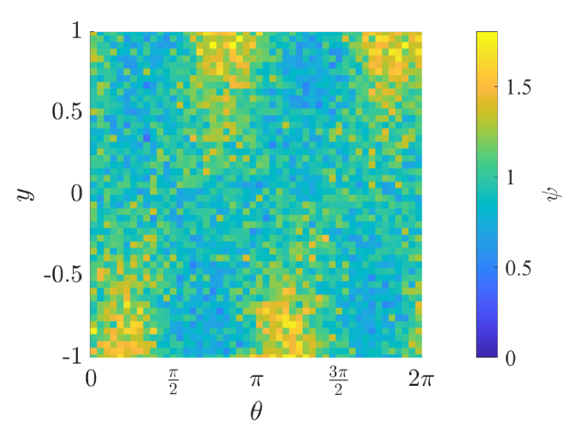
(a)

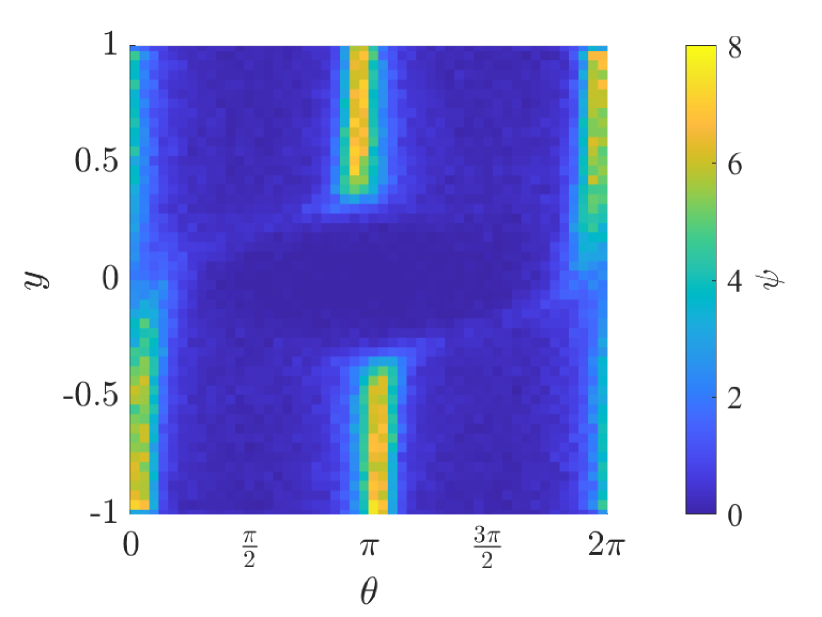
(b)

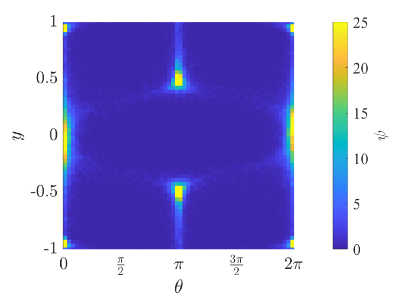
(c)

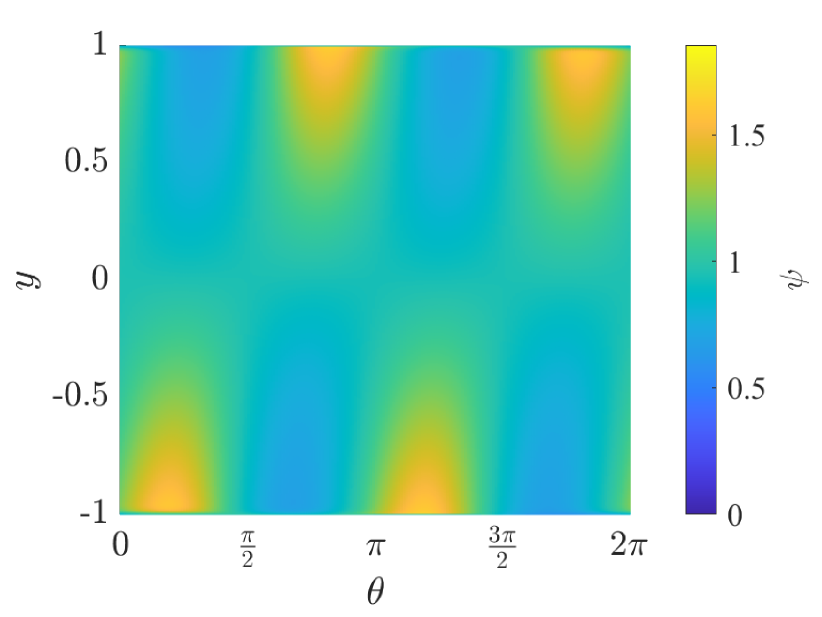
(d)

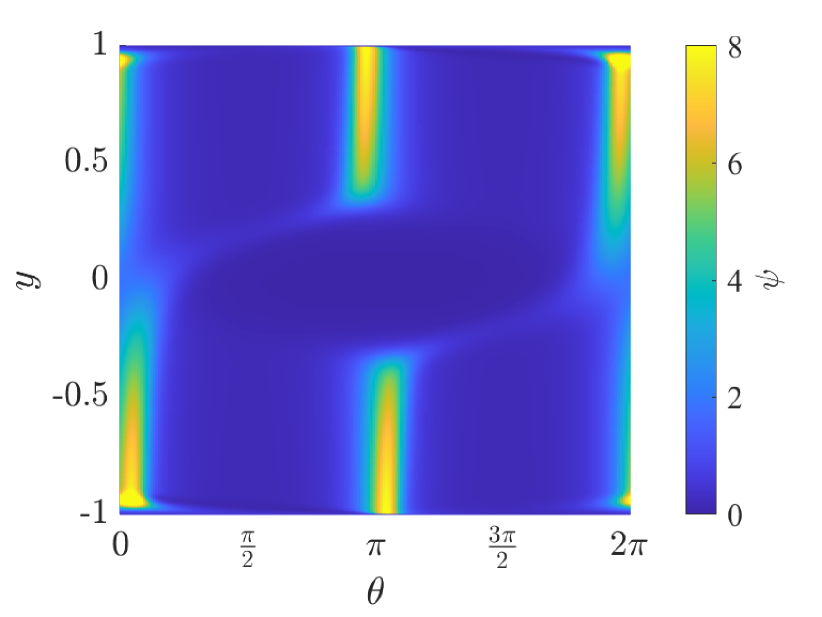
(e)

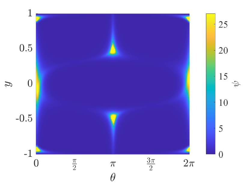
(f)

Figure 5: Comparison of snapshots of bivariate probability density distributions for IBMs at $T=600$ with random wall reflections (a)–(c), to equilibrium probability density distributions for continuum models with constant boundary condition. (a)&(d): $Pe=1$, (b)&(e): $Pe=100$; and (c)&(f): $Pe=10^{4}$.

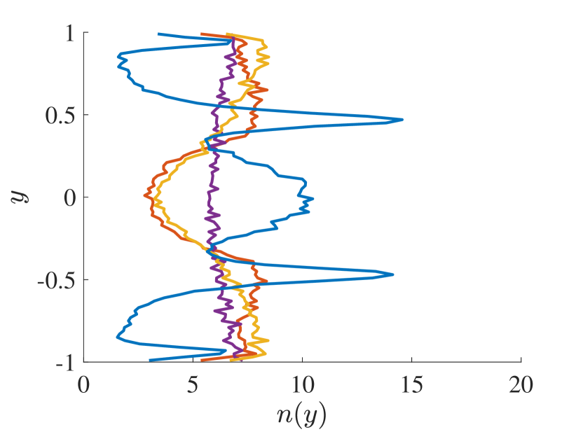
(a)

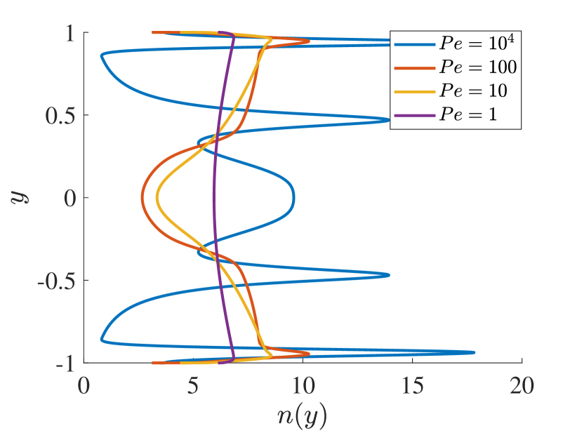
(b)

Figure 6: Cell density distributions for (a): IBM with uniform random wall reflection; and (b): the distribution of continuum model with constant wall distribution. For shape parameters $\beta=0.99$ with $Pe=10^{4}$ (blue), $Pe=100$ (red), $Pe=10$ (yellow) and $Pe=1$ (purple).

3.2.2 Perfectly absorbing boundary (boundary condition $\mathcal{A}$)

Our final boundary condition of interest is the case of perfect wall-attachment, i.e. any swimmer that encounters the wall will adhere to it. For ease of comparing the effect on the bulk dynamics we allow for specular reflection at the top wall ($y=1$) while enforcing a perfectly absorbing bottom wall, such that cell trajectories are terminated upon contact with the bottom wall ($y=-1$). We begin by considering a snapshot of the bivariate probability density distributions $\psi$ at time $T=600$. It is worth noting that given the presence of diffusive effects, given sufficient time, all cells will attach to the bottom wall. In figure 7a ($\beta=-0.99$ and $Pe=1$), the distributions show clear depletion near the bottom wall, as all cells which have been able to encounter the bottom have attached. In figure 7b (for $Pe=100$) fewer cells are captured by the bottom wall by time $T=600$, however, there is a clear depletion, and the accumulation band in the bottom half contains approximately 75% the number of cells as their upper-half channel specular-reflecting counterparts. Finally, figure 7c (for $Pe=10^{4}$) mainly has depletion of cells originating below the deterministic separatrix for wall interactions, as cell diffusion is very small.

In figures 7d-7f, we consider the normalised orientation distributions of the cells which have been absorbed at the bottom wall. In figure 7d we find that in the presence of high diffusion, the wall encounter probability distributions are wide, centred about $\theta_{peak}=3\pi/2$, and the distributions remain unchanged for $T=50,100,600$. For $Pe=100$ in figure 7e, the peak near $\theta=\pi$ continuously increases in time. This localised increase is due to swimmers crossing the yellow deterministic separatrix in figure 7c. The rotational diffusion is sufficiently weak that deterministic effects dominate and cells are quickly captured by the absorbing condition just above $\theta=\pi$. Finally, for figure 7f, we note a similar increase in the peak near $\theta=\pi$. In fact, across figures 7d-f, we find that the peak orientations at which absorptions occurs shifts from $\theta_{peak}=3\pi/2$ towards $\theta_{peak}=\pi$ with decreasing rotational diffusion.

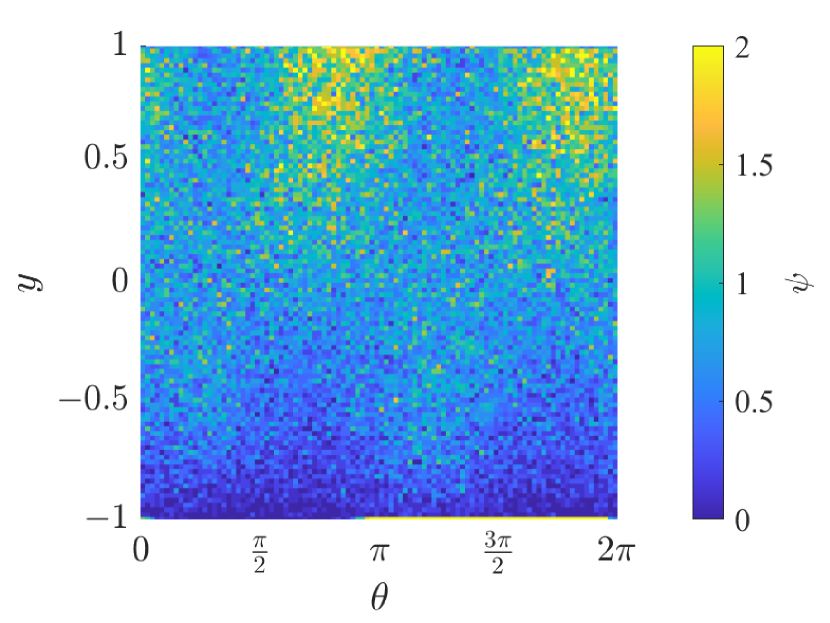
(a)

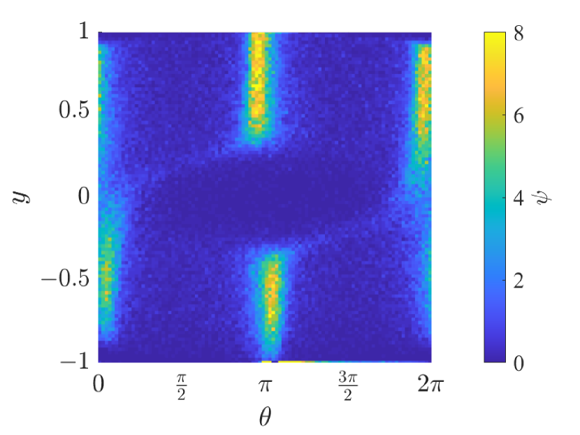
(b)

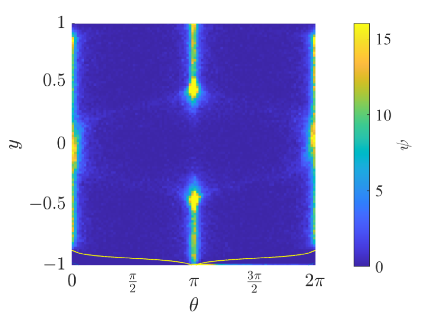
(c)

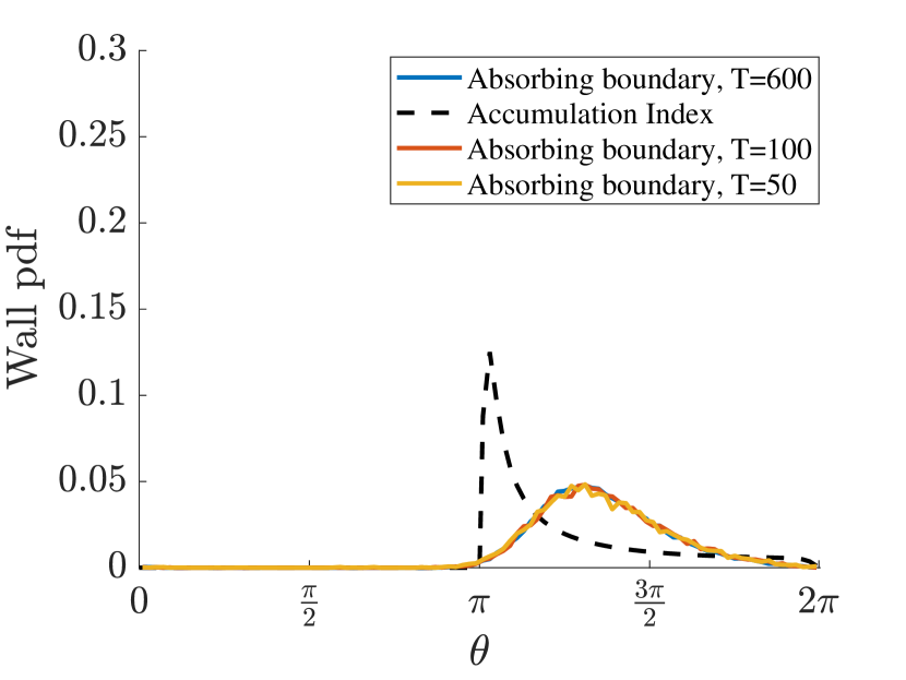
(d)

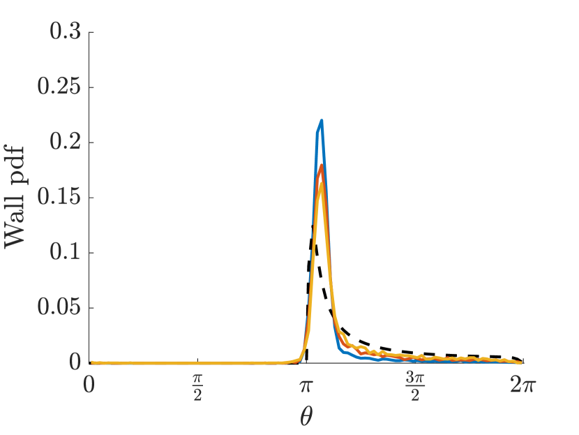
(e)

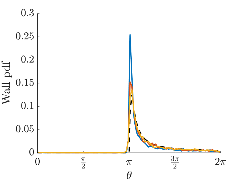
(f)

Figure 7: A snapshot of the effects of a perfectly absorbing wall condition at the bottom wall for an IBM (with dynamics at top wall prescribed by specular reflection) on the bulk dynamics ((a)–(c)) at $T_{run}=600$ $T_{sim}=600$ and on normalised wall orientation probability distributions for $\beta=0.99$ ((d)–(f))for runtimes $T_{run}=50,100,600$$T_{sim}=50,100,600$. The black dashed lines correspond to wall distributions for $\beta=0.99$ as calculated by the accumulation index (see §3.3). (a)&(d):$Pe=1$, (b)&(e):$Pe=100$ and (c)&(f):$Pe=10^{4}$, .

3.3 Deterministic wall approach and underlying dynamics

(a)

(b)

(c)

(a)

(b)

(c)

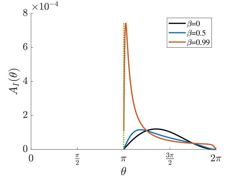
(d)

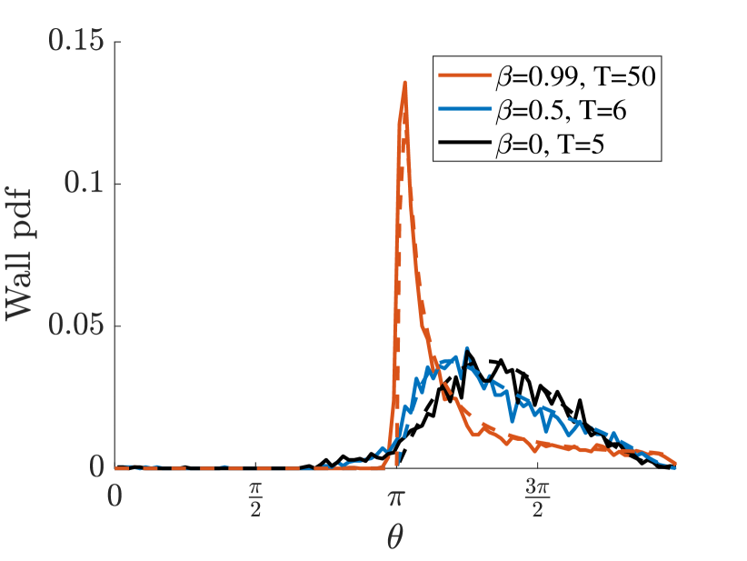
(e)

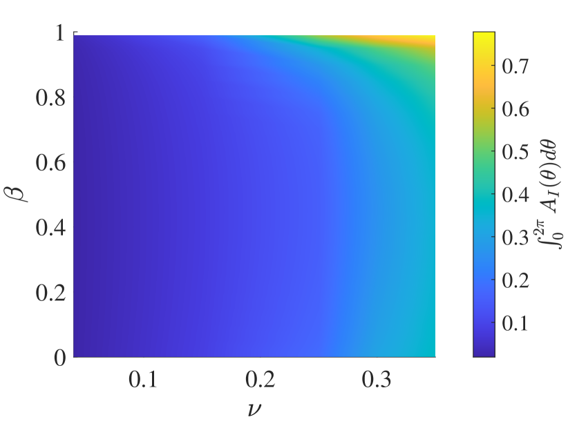
(f)

Figure 9: Deterministic dynamics and the accumulation index. (a) Schematic of the accumulation index; (b) Streamlines at constants of motion for $\nu=0.04$, $\beta=0,0.5,0.99$ (solid black, dashed blue, and dash-dotted red, respectively); (c) Streamlines at constants of motion for $\nu=0.1$, $\beta=0,0.5,0.99$ (solid black, dashed blue, and dash-dotted red, respectively); (d) Accumulation index (proportion of initially uniformly distributed cells in the phase space that are incident upon the bottom wall at angles $\theta$) for $\beta=0,0.2,0.5,0.7,0.99$, for $\nu=0.04$; (e) Distribution of wall interactions with absorbing boundary conditions (solid lines) for $Pe=10^{4}$ for $\beta=0,0.5,0.99$ with $T_{run}=5,6,$ $T_{sim}=5,6,$ and 50, respectively, and the corresponding accumulation index distributions (dashed lines); and (f) Proportion of total area of phase space incident on the bottom wall $\int_{0}^{2\pi}A_{I}(\theta;\beta,\nu)\,\mathrm{d}\theta$ as a function of shape, $\beta$, for various swimming speeds, $\nu$.

While in the previous sections (§LABEL:Sec:Nonunique, §§3.1, §3.2) we considered the equilibrium distributions of a dilute suspension of swimmers in a pressure driven channel flow and the effects of diffusion on wall interaction orientations, in this section we will be focusing on individual deterministic trajectories in such a channel, and how the underlying dynamics of swimmers of different shapes and shears impact their orientations at wall-approach in the $\theta$-$y$ space. This is of particular interest as the individual dynamics inform how suspension interact with the walls, and sheds insights into why swimmers of different geometries are more likely to interact with the walls with different preferred orientations and thereby affect their likelihood of wall attachment and biofilm formation. For this, we consider the deterministic problem, in which we keep the purely deterministic drift term and remove diffusion dynamics, such that

$$\displaystyle{\frac{\mathrm{d}y}{\mathrm{d}t}} =\nu\sin\theta,$$ (20)

$$\displaystyle{\frac{\mathrm{d}\theta}{\mathrm{d}t}} =y(1-\beta\cos 2\theta).$$ (21)

From this, we derive constants of motion for the dynamics (similar to zottl2013periodic), by eliminating time dependence and solving

$$\displaystyle{\frac{\mathrm{d}y}{\mathrm{d}\theta}}=\dfrac{\displaystyle{\frac{\mathrm{d}y}{\mathrm{d}t}}}{\displaystyle{\frac{\mathrm{d}\theta}{\mathrm{d}t}}}=\dfrac{\nu\sin\theta}{y(2-\beta\cos 2\theta)}.$$ (22)

We find constants of motion, $H$, with $y,\theta,\beta$ and $\nu$ dependence, such that

$$H=\dfrac{y^{2}}{2\nu}+\dfrac{1}{\sqrt{2\beta(1+\beta)}}\mathrm{arctanh}\left(\sqrt{\frac{2\beta}{1+\beta}}\cos\theta\right)+{Constant.}$$ (23)

From this we derive the trajectories $y(\theta;H,\beta,\nu)$ in phase space $\theta$–$y$, for any particle with initial condition $(\theta_{0},y_{0})$ and corresponding constant of motion $H$:

$$y(\theta;H,\beta,\nu)=\sqrt{{2\nu}\left(H-\dfrac{1}{\sqrt{2\beta(1+\beta)}}\mathrm{arctanh}\left(\sqrt{\frac{2\beta}{1+\beta}}\cos\theta\right)\right)}.$$ (24)

From the trajectories we extract information regarding the expected wall interactions, trajectory times, and develop a novel accumulation index determining the distribution of expected wall interactions in the case of a uniformly seeded domain. Example trajectories are shown in figure 9(b) for $\nu=0.04$, where $\beta=0,0.5$ and $0.99$. The trajectories of deterministic swimmers can be split into two groups: trajectories which interact with the walls and trajectories which do not. Our interest lies in the former, and we note that each of the wall-interacting trajectories hits the wall at a different angle. The shape of the trajectories themselves are dependent upon the elongation of the swimmers as highlighted in figures 9(b) and 9(c), where the black lines correspond to spherical swimmers ($\beta=0$), the blue-dashed lines correspond to swimmers with shape parameter $\beta=0.5$, and the red dash-dotted lines correspond to $\beta=0.99$. Elongated swimmers undergo increasing strain effects, such that swimmers spend extended times oriented with the flow direction ($\theta=0,\pi$). With increased elongation, the reorientation in phase-space $\left(\displaystyle{\frac{\partial y}{\partial\theta}}\right)$ steepen steepens about $\theta=0$ and $\theta=\pi$, thus leading to a change in total area enclosed by trajectories through $\theta=\pi,y=\pm 1$ and the cell trajectories upon wall approach.

Supposing there is an initial, uniform distribution over the entire phase plane $\theta\times y\in[0,2\pi)\times[-1,1]$, the accumulation index, $A_{I}$, is defined as

$$\int^{\theta+\delta\theta}_{\theta}A_{I}(\theta^{\prime})\,\mathrm{d}\theta^{\prime}=\frac{I_{W}(\theta,\theta+\delta\theta)}{N},$$ (25)

where $I_{W}(\theta,\theta+\delta\theta)$ is the total number of swimmers that interact with the bottom wall at $y=-1$ with orientations ranging in $[\theta,\theta+\delta\theta]$ (see schematic in figure 9(a)), and $N$ is the total number of swimmers. The accumulation indices for orientations of incidence captured in figure 9(d) correspond to the velocity ratio $\nu=0.04$. We find that the distributions for various elongations ($\beta=0,0.5,0.99)$follow the same trends despite a difference in scaling. REWORD??We find that the distributions for various elongations ($\beta=0,0.5,0.99)$ follow the same trends despite a difference in scaling. For a fixed centreline flow velocity, the increased accumulation index for $\nu=0.1$ results from the increased swimming velocity $V_{s}$ enabling swimmers to traverse larger vertical distances prior to shear-induced reorientation. This, in turn, allows larger proportions of swimmers in an initially uniformly distributed domain to interact with the walls.

Further points of interest include the orientation $\theta_{peak}$ at which maximal wall interactions occur. In the accumulation index (figure 9d) there is a shift in the peak interaction orientation $\theta_{peak}$ from $\theta_{peak}\approx 3\pi/2$ to $\theta_{peak}\approx\pi$, with cell elongation. We find similar shape-based shifts in peak wall-interaction orientation with the absorbing boundary condition in figure 9(e).

The absorbing boundary condition distributions are shown to be in agreement with the accumulation index in the case of small rotational diffusion for shape dependent run times $T_{run}$ simulation run times $T_{sim}$ that are sufficiently long to allow cells to encounter the walls. The run times required for optimum matching are shape dependent as elongation affects the duration of Jeffery orbits. The Jeffery orbits, in turn, affect the time it takes for cells with specific initial positions and orientations to to swim and rotate before cells encountering the walls. It is also necessary to limit the simulation run times for matching as the clear shape dependent shift in peak interaction orientations (figure 9(e)) disappears for sufficiently long run times, highlighting the transience of the accumulation index distribution. For low rotational effects (figure 7), for the case of the absorbing boundary condition, the long term peak continuously increases about $\theta=\pi$. Here, the diffusion effects are sufficiently small that once any cells diffuse into Region 1, the deterministic component dominates and they strike the wall close to $\theta=\pi.$ Similar peaks have been observed to grow about $\theta=\pi$ for less elongated swimmers in the long-term. The balance between diffusion and advective domination may also be the underlying reason for shape independence in peak wall interactions observed for non-spherical swimmers in the reflective boundary case (see figures 4(c), 4(f), and 4(i)). In figure 9(f), the total proportion of swimmers which interact with the bottom wall $\int_{0}^{2\pi}A_{I}(\theta)\,\mathrm{d}\theta$ are shown for a range of shape factors and velocity ratios. For small swimming velocities, for swimmers of all considered shape factors, only a small proportion of swimmers are expected to interact with the lower wall due to deterministic effects. The proportion of wall interactions increases monotonically with swimming velocity, and increases fastest for $\beta>0.9$, with over 70% of swimmers interacting with the bottom wall for $\nu>0.3$.

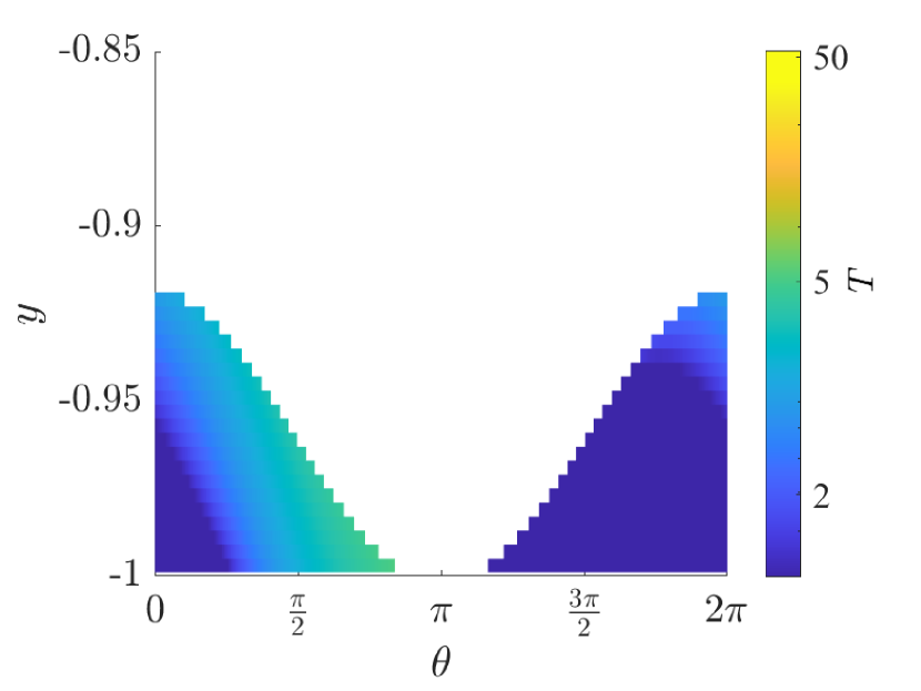
(a)

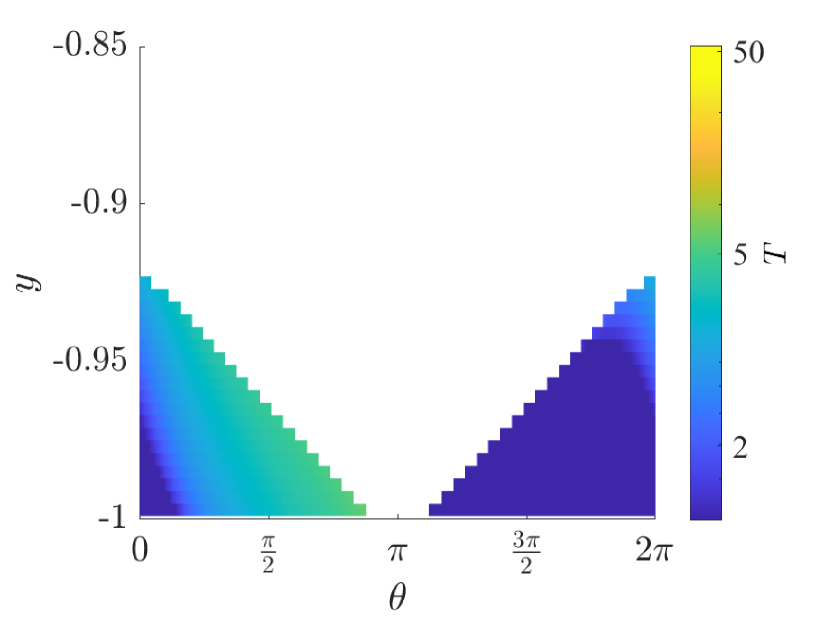
(b)

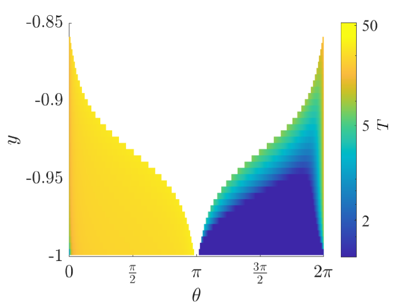
(c)

Figure 10: Shape dependence of time taken for trajectories beginning at $(\theta_{0},y_{0})$ to reach an absorbing wall condition at $y=-1$, $\theta\in[\pi,2\pi)$. From this we can extrapolate the total number of wall interactions by swimmers in the ‘trapped’ domain over a fixed total runtime. For $\nu=0.04$, (a) $\beta=0$, (b) $\beta=0.5$, (a) $\beta=0.99$.

While swimmer shape affects the orientations at which swimmers are most likely to interact with the bottom wall we find that all particle trajectories are not of equal time duration. While separate identical particles on the same trajectories will have the same orbit duration in the deterministic problem, identical particles on different trajectories will have different orbit durations dependent on cell shape and velocity ratio $\nu.$ In figure 10, the colour maps highlight the time taken for a trajectory starting at position $(\theta_{0},y_{0})$ to terminate at the bottom wall (i.e. at $y=-1,\theta\in[\pi,2\pi]$) via an absorbing wall boundary condition. The longest trajectories have durations ranging from $T\approx 6$, for $\beta=0$, to $T\approx 45$, for $\beta=0.99$, indicating that slender, elongated cells can take over seven times longer to complete a single full orbit, compared to spherical cells. This indicates, that the former has over seven times fewer opportunities for wall interactions over a fixed runtime. Although a larger proportion of cells are likely to come into contact with walls at orientation $\theta_{peak}$ (as in figure 9(d)), the particles initially oriented about $\theta=\pi$ have the longest orbit durations, while cells about $\theta=0$ have the shortest trajectories. When considering a Lagrangian perspective, this acts as a limiting factor for the number of wall interactions per interaction orientation. The number of orbits which a particle can undergo over a fixed runtime $T_{run}$ simulation runtime $T_{sim}$ is of biological interest, as it affects the probability of biofilm formation due to increased opportunities for cell attachment. Finally, we note that to match the accumulation index and the perfectly absorbing boundary $\mathcal{A}$ (as shown in figure 9(e)) we took the asymptotic limit to the deterministic problem ($Pe\rightarrow\infty$) for run-times as calculated in figure 10.

4 Conclusions

Using a finite element framework for studying the equilibirium distributions of dilute suspensions of microswimmers we have ascertained that the choice in boundary conditions in continuum modelling is crucial as there exists a coupled relationship between the bulk flow cell dynamics and the boundary dynamics. Though it is known in general that the no-flux boundary condition is non-unique, we note that the choice of constraints in the continuum approximation corresponds to specific different reflective dynamics. We find that a doubly periodic Poiseuille continuum approximation yields a good approximation of wall-bounded Poiseuille dynamics with specular reflection, while a constant boundary approximation in the continuum model yields good agreement with random reflection models. The former is especially noteworthy as this offers justification for the use of doubly periodic Poiseuille flow models like vennamneni2020shear to capture simple bounded domains with a reflective wall condition. Both results further justify the use of these continuum approximations in the study of wall interactions for the case of dilute microswimmer suspensions.

The shape of the swimmers and rotational diffusion experienced by the swimmers is shown to significantly affect the orientation distributions. From a Eulerian perspective, there are no-prefered cell orientations for spherical cells, while more elongated swimmers exhibit a clear preference for orientation up and downstream. This preference has smallest orientational spread for $\beta=0.99$, for which the distributions are most peaked near $\theta={0,\pi}$, with 40% of cells interacting with the walls with incidence angles $\theta\in[\pi-0.25,\pi+0.5]$. From a Langrangian Lagrangian perspective, this is a result of Jeffery orbits realigning elongated swimmers with non-uniform angular velocity with the flow direction. On decreasing the rotational Péclet number, $Pe$, the spread of maximum wall incidence shifts from $\theta_{peak}=\pi$ to $\theta_{peak}=3\pi/2$ as diffusion dominates deterministic dynamics. For the case of an absorbing boundary condition, when decreasing the rotational diffusion, the wall-incidence distributions tend towards the distributions as captured by the novel accumulation index for shape-dependent limited runtimes.

The deterministic dynamics of individual trajectory dynamics in the phase plane $\theta$–$y$ capture the shift in peak orientation distribution from $\theta_{peak}=3\pi/2$ to $\theta_{peak}=\pi$ for spherical to highly elongated swimmers via the accumulation index. The perpendicular approach of spherical swimmers towards surfaces and the parallel approach of elongated swimmers towards walls, have been observed for both Chlamydomonas and bacteria, respectively, in experiments and numerical studies which include hydrodynamic interactions. Our results suggest that the orientational preferences are enhanced by the fundamental bulk behaviours of different shaped swimmers.

We find that in the absence of diffusion, elongated particles take over seven times as long before interacting with the wall compared to a spherical swimmer. It is possible that elongated swimmers, therefore, must maximise each opportunity they have near the wall. Once near a wall, elongation leads to increased resistance to random Brownian rotation allowing swimmers to remain oriented parallel to flows for longer periods which improves their chemotactic sampling accuracy. Additionally, longer periods of alignment with walls allow for longer periods of mechanosensing, which increases the chances of surface attachment being initiated.

While we have considered multiple idealised wall interaction models, true biological wall interactions do not follow pin-ball dynamics, uniformly random reflections, or perfect absorption. For microswimmers in nature, there exist further variables which affect the likelihood of attachment and reorientation like pili attachment location (melville2013type; jain2012type; proft2009pili), chemical signals (wadhams2004making), hydrodynamic stresses (boyle2006quantification; conrad2018confined) and cell deformability (yoshida2020soft). Further experimental data regarding pili, and observed attachment rates at different cell orientations are required to refine the models to specific swimmer types and to draw further conclusions regarding the likelihood and speed of initial biofilm formation.

Declaration of Interests

The authors report no conflict of interest. Do we need to add any further statements for UKRI purposes? data statement??

Appendix A IBM with specular reflection: Origin of the wall depletion region

For the case of the stochastic individual based model regions of accumulation occur in the $\theta$–$y$ phase space, as observed for the doubly periodic Poiseuille flow and the wall-bounded formulation in section 3.1. However, in the case of the wall-bounded distribution with specular reflection at the walls, a drop in cell accumulation occurs around $\theta=0$ at $y=-1$, and $\theta=2\pi$ at $y=1$ which increases with increased run time. This drop in accumulation is found to be a numerical artefact due to the discrete nature of the numerical method in the IBM.

(a)

(b)

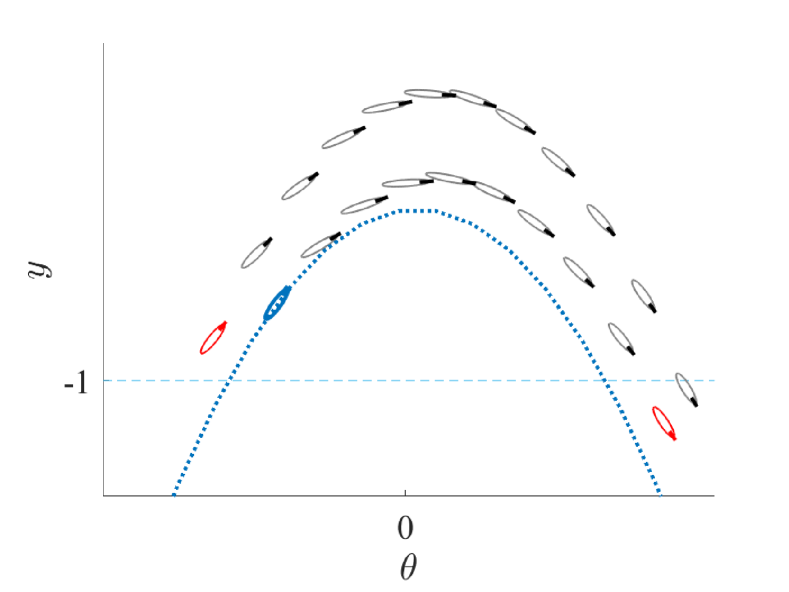
(c)

(d)

(e) Figures to highlight the sensitivity of the IBM to finite time steps, and how these affect the observed boundary interactions. IBM Poiseuille flow, for $\beta=0.99$, $\nu=0.04$. Purely deterministic IBM for $T=600$ in (a) & (b), with (a): $dt=10^{-3}$ and (b): $dt=0.1$. (c): Schematic of trajectory of particle at bottom wall in continuous time (blue dotted line) highlighting the trajectory deviation for particles of finite time step. Red particle on the right overshoots the wall, and is reflected to the red particle on the left. (d): $\psi$ distribution at $\theta=0$ for varying $y$ for dt=0.1 (blue line) and dt=0.001 (red line).

Figure 11: Figures to highlight the sensitivity of the IBM to finite time steps, and how these affect the observed boundary interactions. IBM Poiseuille flow, for $\beta=0.99$, $\nu=0.04$. Purely deterministic IBM for $T=600$ in (a) & (b), with (a): $dt=10^{-3}$ and (b): $dt=0.1$. (c): Schematic of trajectory of particle at bottom wall in continuous time (blue dotted line) highlighting the trajectory deviation for particles of finite time step. Red particle on the right overshoots the wall, and is reflected to the red particle on the left. (d): $\psi$ distribution at $\theta=0$ for varying $y$ for dt=0.1 (blue line) and dt=0.001 (red line). Overshoot error estimate function? Numerical wall interaction angle- analytical wall unteraction angle

To illustrate this, consider the case of a purely deterministic system such that the cells must all follow predetermined trajectories. However, time is a discrete variable in the differential equation. as time is discretised the time steps are of finite size. Over a run time $T=600$, we find a 50% cell depletion in a radius of $2\epsilon(=0.08)$ about $(\theta,y)=(0,-1)$, when increasing step size from $\mathrm{d}t=10^{-3}$ to $\mathrm{d}t=0.1$ as seen in figures 11(a) and 11(b). As shown in the schematic in figure 11(c), if a swimmer (the blue particle) begins on a deterministic trajectory given by the dotted blue line, due to distrete discrete step sizes, the swimmer will gradually stray further from the continuous trajectory with consecutive steps. This effect is compounded when the last step in the orbit overshoot (see the red particle on the right), and undergo specular reflection (the red particle on the left) to a position firmly outside its previous deterministic trajectory. With each cycle of reflection, the particle moves further from $\theta=0$, and create an artificial cell depletion region. In figure 11(d) we consider the distribution $\psi$ in space $y$ at $\theta=0$, and find stark cell depletion after time $T=600$ for $\mathrm{d}t=0.1$ at the walls. As these cells move away from the wall due to numerical leaking, they accumulate and form an artificially large peak around $y=\pm 0.86$ for $T=600$.

Appendix B Two-phase cell density distribution

(a)

(b)

Figure 12: Two stage dynamics of IBM for $\beta=0.99$, $\nu=0.04$, $Pe=10^{4}$, $Pe=10^{6}.$ (a) Time lapse bivariate probability density distributions highlighting transition from initial formation of bands of accumulation, to cell depletion of cells at $(\theta,y)=(\pi,-1)$ due to long time diffusive effects. (b) Probability density distribution cross section at $y=-1$ in time, highlighting cell depletion in time.

For the case of low rotational diffusion dynamics (high $Pe$) with high elongation ($\beta=0.99$), the individual based method does not reach equilibrium by $T=600$ (irrespective of boundary condition). For the case of the doubly periodic Poiseuille flow IBM, we instead find that the distribution reaches an intermediate phase distribution, during which cells accumulate in regions of almost uniform distribution concentration from $y=-1.5$ to $y=-0.5$ in figure 12(a)(i). After this initial, intermediate distribution, after an extended run time, translational and rotation diffusion effects cause cells to disperse away from $y=-1$ and accumulate near $y=-0.4$ and $y=-2$ at $\theta=\pi$. This is also seen in the gradual decrease in intensity at the centre of accumulation bands in $y$ from figures 12(a)(ii) to 12(a)(iv). Similarly, for $\theta=0$ cells disperse away from $y=-1$ to peaks at $y=0$ and $y=-1.4$.

The gradual decrease in cells at the walls is also evidenced by taking a cross section of the probability distribution $\psi$ at $y=-1$ (figure 12(b)), highlighting the time dependent monotic monotonic decrease in the amplitude of the distributions.

Appendix C Cell wall interaction origins

(a)

(b)

(c)

(d)

(e)

(f)

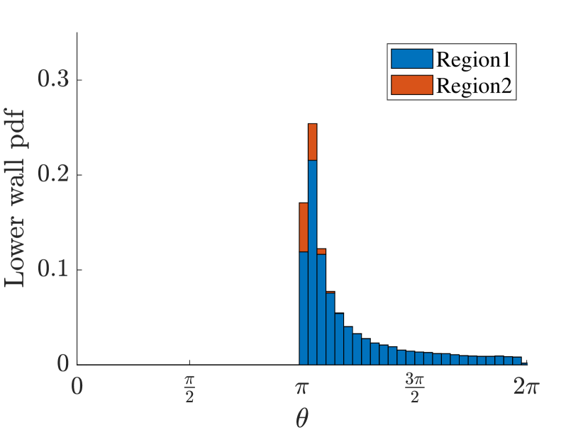
(g)

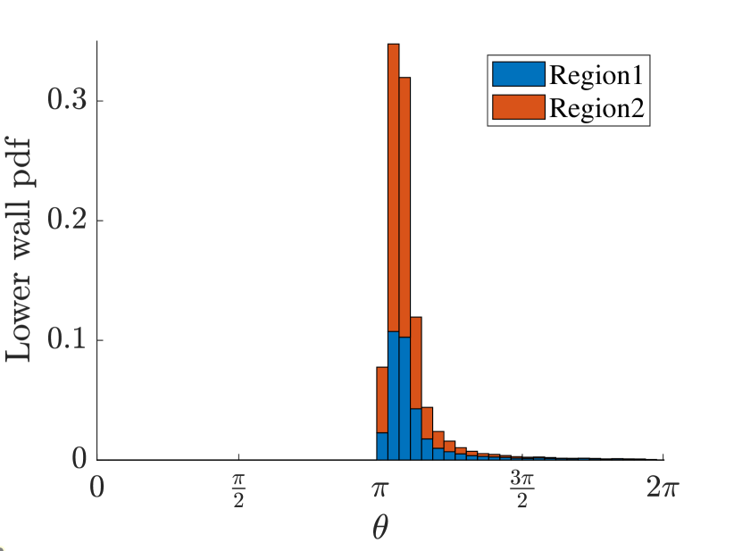
(h)

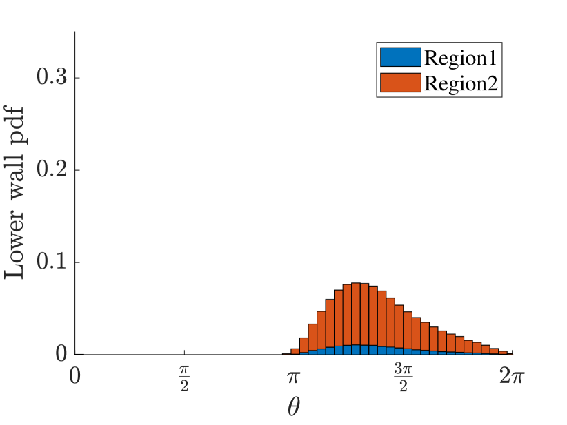
(i)

(j)

Figure 13: The impact of rotational diffusion the distributions of micro-swimmers which interact with the wall, and how the Péclet number affects what proportion of swimmers originate in region 1 (below the yellow deterministic separatrix from figure 8(e)). i.e. How important are these deterministically ‘trapped’ areas in the presence of rotational diffusion? Stacked probability distribution of angle of incidence for particles striking the lower wall ($y=-1$), for $\nu=0.04$ and $Pe_{T}=10^{6}$. The blue distribution correspond to particles which are expected to strike the wall in the absence of diffusive effects, and the red, correspond to particles who would not strike the bottom wall in the absence of diffusive effects. For $\beta=0$, (a)$Pe=10000$, (b)$Pe=100$, and (c)$Pe=1$; for $\beta=0.5$, (d)$Pe=10000$, (e)$Pe=100$, and (f)$Pe=1$; and for $\beta=0.99$, (g)$Pe=10000$, (h)$Pe=100$, and (i)$Pe=1$. (j) Proportion of wall interactions from region 1 for varying $\beta$ and Péclet numbers.

In the idealised case, in the absence of all diffusion, the trajectories of cells with specular reflection are predetermined. However, microswimmers like bacteria will experience diffusive effects in sufficciently weak flows, and therefore cross the deterministic streamlines. For a fixed simulation runtime, $T_{sim}=600$ we quantify the effect of increased diffusion on the cells interacting with the walls (figure 13). For this we consider stacked probability distributions which distinguish between cell–wall interactions based on initial positions $(\theta_{0},y_{0})$. Suppose the phase space domain can be split into two regions via a separatrix (e.g. the yellow separatrix in figure LABEL:Fig3c for $\beta=0.99$): the lower region where all cells (in the absence of diffusion) must interact with the wall, and upper region where all cells will not interact with the wall. The particles which originate in the region where the deterministic trajectories expected to have deterministic wall interactions are tracked as ‘region 1’ particles given in blue and those which would not, are tracked as ‘region 2’ particles given in red.

For $Pe=10^{4}$ (figures 13(a), 13(d) and 13(g)), for $\beta=0,0.5,0.99$, respectively, the orientation distribution peaks tend toward $\theta\rightarrow\pi$ as $\beta\rightarrow 1$. While the transition for the low rotational diffusion case is comparable to the shift in peak captured via the accumulation index, the tails for larger $\theta$ are flatter, and the peak for $\beta=0$ (figure 13(a)) occur at lower incident orientations, again caused by numerical leaking. For low diffusion, over 80% of all wall interaction originate from region 1, and decrease monotonically with $Pe$, irrespective of swimmer shape (see figure 9(f)). An increase in rotational diffusivity (figures 13(b), 13(e), and 13(h)) shift the peaks of the distribution $\theta_{peak}\rightarrow 3\pi/2$, and decreases the size of the peak with a decrease in $\beta$. A symmetric distribution about $\theta=3\pi/2$ is only possible as $\beta\rightarrow 0$, $Pe\rightarrow 0$.