Broadcasting solutions on networked systems of phase oscillators

Abstract

Networked systems have been used to model and investigate the dynamical behavior of a variety of systems. For these systems, different levels of complexity can be considered in the modeling procedure. On one hand, this can offer a more realistic and rich modeling option. On the other hand, it can lead to intrinsic difficulty in analyzing the system. Here, we present an approach to investigate the dynamics of Kuramoto oscillators on networks with different levels of connections: a network of networks. To do so, we utilize a construction in network theory known as the join of networks, which represents “intra-area” and “inter-area” connections. This approach provides a reduced representation of the original, multi-level system, where both systems have equivalent dynamics. Then, we can find solutions for the reduced system and broadcast them to the original network of networks. Moreover, using the same idea we can investigate the stability of these states, where we can obtain information on the Jacobian of the multi-level system by analyzing the reduced one. This approach is general for arbitrary connection schemes between nodes within the same area. Finally, our work opens the possibility of studying the dynamics of networked systems using a simpler representation, thus leading to a better understanding of the dynamical behavior of these systems.

I Introduction

Networked systems have been used to model and understand collective behaviors of several systems [1, 2, 3]. Examples can be found spanning from neuroscience [4] to ecology [5] to physical systems, like power-grids [6, 7, 8]. These systems can be understood as single, undirected small networks, or networks of networks, or even networks with higher-order interactions [9, 10]. In this context, one important approach to improve the modeling of real systems is given by networks with different levels of connections [11, 12, 13, 14]. This approach allows the study of important systems such as spreading processes [15], animal behavior [16], neural dynamics [17, 4], and synchronization phenomena [18, 19]. On the other hand, the addition of an extra level of connections makes the analysis process more complicated, especially for analytical and mechanistic insights. In this paper, we present an approach that offers a simplified way to analyze the dynamics of these networks, which allows us to obtain equilibrium points and analyze the stability for a large class of such systems.

Here, we focus particularly on systems that can be understood as a network of networks [13, 14, 20]. In this case, the system can have two levels of connections: on the first level, there are connections within each sub-network; on the higher level, there are connections between the sub-networks. This is similar to multilayer networks [11, 12]. In our case, though, we consider the same nature of coupling in all levels, i.e. the function describing the interaction is the same. We then consider different scale factors and connection architectures in each level. Due to these reasons, we use the two terms a network of networks and a multi-level network interchangeably throughout this article.

Based on the framework developed in [21, 22, 23], we can represent a network of networks, a multi-level system, by a join of matrices containing information about the connections in different levels. We then introduce a reduced representation of the system, which has a clear connection with the join matrix that represents the multi-level network. Thus, this reduced system allows us to study the dynamics of the sophisticated system in a simpler way. Then, we can find solutions for the reduced system and broadcast them to the original networks. In other words, we can use our reduced representation of the dynamical system to find solutions and then spread this dynamics to the multi-level network. This kind of approach has been used in the literature for the study of the dynamical behavior of these networks under different perspectives. For instance, Schaub et al. have introduced a comprehensive framework to study multilayer networks using a similar idea [24]. Further, cluster synchronization and its stability have been studied on these networks considering phase oscillators [25, 26].

Here, among various applications, our approach offers a direct way to find and analyze equilibrium points in a network of networks with an arbitrary number of sub-networks and arbitrary connection architecture (adjacency matrices) for nodes within the same sub-network. To study this problem, we consider the individual dynamics of each node given by the Kuramoto model [27, 28, 29], so each node is represented by a phase oscillator. The Kuramoto model is a central model for the studying of synchronization and the collective behavior of several systems. It has been used in problems spanning from social interactions [30] to biology [31, 32] and physics [33, 34]. Particularly, a variety of synchronization phenomena and spatiotemporal patterns has been observed in Kuramoto systems: phase synchronization [29, 35], remote synchronization [36], twisted states [37, 38], chimera states [39, 40], and Bellerophon states [41].

Furthermore, by considering the properties of joins of matrices and the idea of representing the multi-level network by the reduced system, we can investigate into the stability of equilibrium points for Kuramoto oscillators on these networks. When the solutions for the multi-level systems are obtained through the broadcasting process from the reduced system, we have found a relation between the Jacobian of both systems. In this sense, we can evaluate the spectrum of a simpler matrix - representing the reduced systems - and obtain information on the stability of the equilibrium points for the more sophisticated, multi-level networks.

In this paper, we first introduce Kuramoto oscillators on a network of networks and expose our approach with the reduced system and also show how we broadcast solutions to the multi-level system - Sec. II; we extend the approach to the linear stability analysis of multi-level networks - in Sec. III; in addition to this, we show numerical simulations and examples of Kuramoto network of networks and their reduced version, which corroborate the main approach introduced in this paper - Sec. IV; finally, we discuss the results presented here and their implications, and draw our conclusions - Sec. V.

II Kuramoto oscillators on a network of networks

The Kuramoto model [27, 28, 29] can be defined as the dynamical system governed by the equation

$$\frac{d\theta_{i}}{dt}=\omega_{i}+\sum_{j=1}^{\mathcal{N}}A_{ij}\sin(\theta_{j}-\theta_{i}),$$ (II.1)

where $\theta_{i}\in[-\pi,\,\pi]$ is the phase of the $i^{\mathrm{th}}$ oscillator, $\omega_{i}$ is its natural frequency, $\mathcal{N}$ is the number of oscillators in the system, and $A_{ij}$ are the elements of the weighted adjacency matrix that represents the connections of this system. That is, $A_{ij}=0$ if nodes $i$ and $j$ are not connected, and $A_{ij}>0$ if nodes $i$ and $j$ are connected. Here, we consider the case where all oscillators have the same natural frequency $\omega_{i}=\omega$ for all $i\in[1,\,\mathcal{N}]$.

II.1 Kuramoto model

For a network of networks, we can consider two levels of interactions: intra-area (within each sub-network) and inter-are (between sub-networks) connections. In this case, the Kuramoto model for the $i^{\mathrm{th}}$ oscillator in the $l^{\mathrm{th}}$ sub-network can be written as:

$$\frac{d(\bm{\theta}_{l})_{i}}{dt}=\omega+\underbrace{\sum_{j=1}^{N}(\bm{A}_{ll})_{ij}\sin((\bm{\theta}_{l})_{j}-(\bm{\theta}_{l})_{i})}_{\mathrm{intra-area}}+\underbrace{\sum_{k=1,k\neq l}^{M}\sum_{j=1}^{N}(\bm{A}_{lk})_{ij}\sin((\bm{\theta}_{k})_{j}-(\bm{\theta}_{l})_{i})}_{\mathrm{inter-area}},$$ (II.2)

where $i,j\in[1,\,N]$ and $l,k\in[1,\,M]$, $M$ being the number of sub-networks and $N$ the number of nodes in each one. Here, the coupling strength between two oscillators can assume different values based on the sub-network these oscillators belong to. Moreover, it is important to emphasize that the intra-area coupling considers the coupling between oscillators within a given sub-network, where we consider that each one has $N$ oscillator; the inter-area coupling considers the coupling between oscillators in different sub-networks.

In this paper, on the other hand, we consider a different representation of a network of networks system. Here, we use properties of joins of matrices to describe Kuramoto oscillators on multi-level networks as:

$$\frac{d\theta_{i}}{dt}=\omega+\sum_{j=1}^{NM}A_{ij}\sin(\theta_{j}-\theta_{i}),$$ (II.3)

where now $i\in[1,\,NM]$, such that:

$$\bm{\theta}=(\underbrace{\theta_{1},\theta_{2},\cdots,\theta_{N}}_{1^{\mathrm{st}}\mathrm{area}},\underbrace{\theta_{N+1},\theta_{N+2},\cdots,\theta_{2N}}_{2^{\mathrm{nd}}\mathrm{area}},\cdots,\underbrace{\theta_{N(M-1)+1},\theta_{N(M-1)+2},\cdots,\theta_{NM}}_{M^{\mathrm{th}}\mathrm{area}}).$$ (II.4)

The adjacency matrix describing the multi-level system is the $NM\times NM$ matrix:

$$\bm{A}=\left(\begin{array}[]{c|c|c|c}\bm{A}_{11}&\bm{A}_{12}&\cdots&\bm{A}_{1M}\\ \hline\cr\bm{A}_{21}&\bm{A}_{22}&\cdots&\bm{A}_{2M}\\ \hline\cr\vdots&\vdots&\ddots&\vdots\\ \hline\cr\bm{A}_{M1}&\bm{A}_{M2}&\cdots&\bm{A}_{MM}\end{array}\right),$$ (II.5)

where $\bm{A}_{lk}$ is a $N\times N$ matrix, which describes the connections between the oscillators in the $l^{\mathrm{th}}$ and $k^{\mathrm{th}}$ areas (sub-networks). In case $l=k$, the block represents the intra-area connections in the $l^{\mathrm{th}}$ area. In case $l\neq k$, the block represents the inter-area connections between oscillators in areas $l$ and $k$. Note that in our treatment these matrices absorb the information about the coupling strength. Here, our approach is able to handle multi-level networks where the coupling strength between two different areas (sub-networks) can be different given two different areas. This means that the coupling strength between the areas $l$ and $k$ can be different than the coupling strength between areas $l$ and $k+1$.

For details on the joins of matrices and on the mathematical background of our approach, see [21, 22, 23].

II.2 Reduced Kuramoto model and broadcasted solutions

In this paper we focus on networks satisfying a regularity condition: namely that the off-diagonal blocks $\bm{A}_{lk}$ for $l\neq k$ have the same row sum (that is, they are row-regular, or semimagic, matrices, [22]). In terms of the Kuramoto model, this assumption means that, for any pair of areas, each oscillator in the first sub-network is connected with the same number of oscillators in the other sub-network. To investigate the dynamics of such a system, we introduce an auxiliary reduced $M\times M$ network, in which each sub-network of the original system is condensed into one global oscillator. More concretely, the reduced system is described by the adjacency matrix

$$\bar{\bm{A}}=\begin{pmatrix}r_{\bm{A}_{11}}&r_{\bm{A}_{12}}&\cdots&r_{\bm{A}_{1M}}\\ r_{\bm{A}_{21}}&r_{\bm{A}_{22}}&\cdots&r_{\bm{A}_{2M}}\\ \vdots&\vdots&\ddots&\vdots\\ r_{\bm{A}_{M1}}&r_{\bm{A}_{M2}}&\cdots&r_{\bm{A}_{MM}}\end{pmatrix},$$ (II.6)

where $r_{\bm{A}_{lk}}$ is the row sum of $\bm{A}_{lk}$. At this point, it is important to emphasize that these matrices have information about the coupling strength for the intra-area and inter-area cases, thus the line sum captures this information.

We can now define the reduced Kuramoto model:

$$\frac{d\bar{\theta}_{i}}{dt}=\omega+\sum_{j=1}^{M}\bar{A}_{ij}\sin(\bar{\theta}_{j}-\bar{\theta}_{i}),$$ (II.7)

where now $i\in[1,\,M]$, and $\bar{\theta}_{i}\in[-\pi,\pi]$ is the phase of an oscillator representing the $i$th sub-network. We emphasize that the main diagonal of $\bar{\bm{A}}$ does not affect the dynamics of the system, since $\sin(\bar{\theta}_{i}-\bar{\theta}_{i})=0$ thus not having an effect on the dynamics of the Kuramoto networks. Therefore, in the following, we often make the harmless identification

$$\bar{\bm{A}}=\begin{pmatrix}r_{\bm{A}_{11}}&r_{\bm{A}_{12}}&\cdots&r_{\bm{A}_{1M}}\\ r_{\bm{A}_{21}}&r_{\bm{A}_{22}}&\cdots&r_{\bm{A}_{2M}}\\ \vdots&\vdots&\ddots&\vdots\\ r_{\bm{A}_{M1}}&r_{\bm{A}_{M2}}&\cdots&r_{\bm{A}_{MM}}\end{pmatrix}\simeq\begin{pmatrix}0&r_{\bm{A}_{12}}&\cdots&r_{\bm{A}_{1M}}\\ r_{\bm{A}_{21}}&0&\cdots&r_{\bm{A}_{2M}}\\ \vdots&\vdots&\ddots&\vdots\\ r_{\bm{A}_{M1}}&r_{\bm{A}_{M2}}&\cdots&0\end{pmatrix}.$$ (II.8)

The Kuramoto network on the multi-level system - Eq. (II.3) - represented by $\bm{A}$ - Eq. (II.5) - and the Kuramoto network on the reduced system - Eq. (II.7) - represented by $\bar{\bm{A}}$ - Eq. (II.6) - have the an equivalent dynamics. Thus, we can use the reduced system to better understand the dynamics on the more sophisticated, multi-level network.

More precisely, solutions for the reduced system can be broadcasted to the original network: given a solution of the reduced Kuramoto model:

$$\bar{\bm{\theta}}^{\ast}=(\bar{\theta}_{1}^{\ast},\bar{\theta}_{2}^{\ast},\cdots,\bar{\theta}_{M}^{\ast}),$$ (II.9)

then

$$\bm{\theta}^{\ast}=(\underbrace{\bar{\theta}_{1}^{\ast},\bar{\theta}_{1}^{\ast},\cdots,\bar{\theta}_{1}^{\ast}}_{1^{\mathrm{st}}\mathrm{area}},\underbrace{\bar{\theta}_{2}^{\ast},\bar{\theta}_{2}^{\ast},\cdots,\bar{\theta}_{2}^{\ast}}_{2^{\mathrm{nd}}\mathrm{area}},\cdots,\underbrace{\bar{\theta}_{M}^{\ast},\bar{\theta}_{M}^{\ast},\cdots,\bar{\theta}_{M}^{\ast}}_{M^{\mathrm{th}}\mathrm{area}}),$$ (II.10)

is the corresponding broadcasted solution of the multi-level system described by $\bm{A}$.

Moreover, we note the dependence of the dynamics on the coupling strength. The inter-area coupling controlled by $\epsilon$ is also presented in the reduced system, see Eq. (II.6). So, if we consider an equivalent initial state, both systems evolve to the equivalent final state. However, the stronger the coupling, the faster the transition, which we summarize in the following proposition whose proof follows from direct calculations (valid for nonzero coupling only):

Proposition II.1.

Suppose $\bar{\bm{\theta}}^{\ast}=(\bar{\theta}_{1}^{\ast},\bar{\theta}_{2}^{\ast},\cdots,\bar{\theta}_{M}^{\ast})$ is a solution of the Kuramoto model

$$\dot{\theta}_{i}=\epsilon\sum_{j}A_{ij}\sin(\theta_{j}-\theta_{i}),$$

with intial condition $\bm{\theta}(0)=\bm{\theta}_{0}.$ Let $\bm{\psi}(t)=\bar{\bm{\theta}}^{\ast}\big{(}\frac{\epsilon^{\prime}}{\epsilon}t\big{)}$. Then $\bm{\psi}(t)$ is a solution of the Kuramoto model

$$\dot{\psi}_{i}=\epsilon^{\prime}\sum_{j}A_{ij}\sin(\psi_{j}-\psi_{i}),$$

with the same initial condition $\bm{\psi}(0)=\bm{\theta}_{0}.$

Remark II.2.

We note that the idea presented in this section about the correspondence between the network of networks and the reduced system is valid even when the sub-networks have a different number of nodes. In this case, $\bm{A}$ would be a $\mathcal{M}\times\mathcal{M}$ matrix, where $\mathcal{M}=N_{1}+N_{2}+\cdots+N_{M}$. We presented here the version where the sub-network have the same number of nodes $N$ for simplicity purpose.

II.3 Kuramoto order parameter

In order to characterize the dynamical behavior of the system, we use the Kuramoto order parameter [29, 28]. The order parameter for the multi-level system is defined as

$$R(t)=\frac{1}{NM}\left|\sum\limits_{j=1}^{NM}\exp{(\mathrm{i}\theta_{j}(t))}\right|,$$ (II.11)

where $\theta(t)$ is given by Eq. (II.3). Here, $R(t)=1$ means that all oscillators in all sub-networks have the same phase at a given time $t$, which is defined as phase synchronization. If the oscillators are not phase synchronized, the order parameter is less than $1$. For the asynchronous behavior, $R$ assumes residual values. When the system is on a phase-locking solution, also called a twisted state, $R(t)=0$.

We also measure the level of synchronization of the Kuramoto network on the reduced representation using the Kuramoto order parameter. In this case, the order parameter is written as

$$\bar{R}(t)=\frac{1}{M}\left|\sum\limits_{j=1}^{M}\exp{(\mathrm{i}\bar{\theta}_{j}(t))}\right|,$$ (II.12)

where $\bar{R}(t)=1$ means the reduced system is phase synchronized at time $t$, an asynchronous behavior leads to a residual value of $\bar{R}$, and if the reduced system has a phase-locking solution (“twisted state”), then $\bar{R}=0$.

By the definition of the broadcasted solution and direct calculations, we have the following proposition.

Proposition II.3.

Suppose that $\bar{\bm{\theta}}^{\ast}$ is a solution of the Kuramoto model on $\bar{\bm{A}}$ and $\bm{\theta}^{\ast}$ is the corresponding broadcasted solution of the Kuramoto model on $\bm{A}.$ Then the two systems have the same Kuramoto order parameter for all times: $R(t)=\bar{R}(t),\,t\geq 0.$

III Stability of equilibrium points

We now propose to analyze the existence and stability of some equilibria for a network of networks through our knowledge of the existence and stability properties of equilibria in the reduced system. Of course, there is a loss in complexity when considering the reduced system and we cannot guarantee that its analysis provides a full picture of the whole multi-level system. However, we show that some crucial information can be obtained from the reduced system by simply broadcasting a known solution thereof to the multi-level network.

In this section, we require that connections between each pair of connected areas are dense, which we approximate by a mean-field (or all-to-all) coupling. In other words, we assume that if layers $l$ and $k$ are connected, then each node in area $l$ is connected to each node in area $k$. As we demonstrate later, we need to consider this assumption to utilize some known results from spectral graph theory when we analyze the correspondence between the multi-level system and the reduced one. Whereas these assumptions formally restrict the applicability of our method, they still cover a rather wide class of networked systems. It is furthermore quite standard to consider identical coupling strength within a networked system and to approximate unknown or uncertain couplings by mean-field interactions [42, 43, 44, 45, 46]. Formally, the above assumptions translate as:

1. $\bm{A}_{ll}$ is the adjacency matrix of an undirected, connected, weighted graph with positive weights.

2. For $l\neq k$, $\bm{A}_{lk}=\epsilon_{lk}\bm{1}_{N}$ where $\bm{1}_{N}$ is a matrix $N\times N$ with all entries equal to $1$.

As observed in the previous section, the (simpler) reduced system can be used to study the dynamics of the multi-level network. In particular, equilibrium points of the reduced system can be broadcast to equilibrium points of the multi-level one.

However, for stability analysis, we cannot extend the idea in a straightforward way. The reason is that a neighborhood of an equilibrium point for the network of networks $\bm{\theta}^{\ast}$ is $NM$-dimensional, while a neighborhood of an equilibrium point for the reduced system $\bm{\bar{\theta}}^{\ast}$ is $M$-dimensional. Broadcasting the neighborhood of $\bar{\bm{\theta}}^{\ast}$

$$B_{\varepsilon}(\bar{\bm{\theta}}^{\ast})=\left\{\bar{\bm{\theta}}^{\ast}+\bm{\varepsilon}\leavevmode\nobreak\ |\leavevmode\nobreak\ \|\bm{\varepsilon}\|_{2}<\varepsilon\right\}\,,$$ (III.1)

to the multi-level system yields an $M$-dimensional subset of the $NM$-dimensional neighborhood $B_{\varepsilon}(\bm{\theta})$.

In order to perform a stability analysis of the broadcasted fixed point, one needs a more in-depth analysis of the Jacobian matrix. Fortunately, we show that such an analysis can still be performed, and leverages our knowledge of the fixed point for the reduced system.

In order to study the stability of these solutions we can use the Jacobian of each system. Here we denote the Jacobian for the multi-level system at the equilibrium point $\bm{\theta}^{\ast}$ as $J(\bm{\theta}^{\ast})=J_{\bm{A}}(\bm{\theta}^{\ast})$, and the Jacobian for the reduced system at the equilibrium point $\bar{\bm{\theta}}^{\ast}$ as $J(\bar{\bm{\theta}}^{\ast})=J_{\bar{\bm{A}}}(\bar{\bm{\theta}}^{\ast})$.

We first recall the matrix $\bar{\bm{A}}$, defined in Eq. (II.6). Then, we notice that main diagonal of $\bar{\bm{A}}$ does not affect the dynamics of the system (since $\sin(\bar{\theta}_{i}-\bar{\theta}_{i})=0$), so we can write the matrix as

$$\bar{\bm{A}}=\begin{pmatrix}0&r_{\bm{A}_{12}}&\cdots&r_{\bm{A}_{1M}}\\ r_{\bm{A}_{21}}&0&\cdots&r_{\bm{A}_{2M}}\\ \vdots&\vdots&\ddots&\vdots\\ r_{\bm{A}_{M1}}&r_{\bm{A}_{M2}}&\cdots&0\end{pmatrix},$$ (III.2)

where, by definition, $r_{\bm{A}_{ij}}=N\epsilon_{ij}$. Based on this matrix, we can now write the Jacobian for the reduced system as

$$J(\bar{\bm{\theta}}^{\ast})=\begin{pmatrix}-\lambda_{1}&r_{\bm{A}_{12}}\cos(\bar{\theta}^{\ast}_{2}-\bar{\theta}^{\ast}_{1})&\cdots&r_{\bm{A}_{1M}}\cos(\bar{\theta}^{\ast}_{M}-\bar{\theta}^{\ast}_{1})\\ r_{\bm{A}_{21}}\cos(\bar{\theta}^{\ast}_{1}-\bar{\theta}^{\ast}_{2})&-\lambda_{2}&\cdots&r_{\bm{A}_{2M}}\cos(\bar{\theta}^{\ast}_{M}-\bar{\theta}^{\ast}_{2})\\ \vdots&\vdots&\ddots&\vdots\\ r_{\bm{A}_{M1}}\cos(\bar{\theta}^{\ast}_{1}-\bar{\theta}^{\ast}_{M})&r_{\bm{A}_{M2}}\cos(\bar{\theta}^{\ast}_{2}-\bar{\theta}^{\ast}_{M})&\cdots&-\lambda_{M}\end{pmatrix},$$ (III.3)

where

$$\lambda_{i}=\sum_{j=1,j\neq i}^{M}r_{\bm{A}_{ij}}\cos(\bar{\theta}^{\ast}_{j}-\bar{\theta}^{\ast}_{i}).$$ (III.4)

In particular, the above Jacobian matrices are semimagic square matrices with line sum zero.

In order to compute the Jacobian for the multi-level system $J(\bm{\theta}^{\ast})$, we first recall the definition of the Laplacian. For an undirected weighted graph $H$ with adjacency matrix $\bm{B}_{H}$ and degree matrix $\bm{D}_{H}$, the Laplacian is defined as:

$$\bm{L}_{H}=\bm{D}_{H}-\bm{B}_{H}.$$ (III.5)

We note that, as long as $H$ is undirected, $\bm{L}_{H}$ is always a symmetric semi-magic square matrix (with row sum equal to zero). Regarding the spectrum of $\bm{L}_{H}$, we have the following proposition. We emphasize that this proposition has been studied and demonstrated already in [47]. We show this proposition and its proof here for completeness.

Proposition III.1.

Let $\bm{L}_{H}$ be the weighted Laplacian matrix of an undirected, connected, weighted graph $H$. Then $\bm{L}_{H}$ has a unique zero eigenvalue and all other eigenvalues are strictly positive.

Proof.

By Gershgorin’s Discs Theorem [48, Theroem 6.1.1], all eigenvalues of $\bm{L}_{H}$ are nonnegative. Note also that the eigenvectors of $\bm{L}_{H}$ form an orthonormal basis of $\mathbb{R}^{n}$, because $\bm{L}_{H}$ is symmetric. Now assume that $\bm{v}$ is an eigenvector of $\bm{L}_{H}$ associated with the eigenvalue $0$. Then,

$$0 =\bm{v}^{\top}\bm{L}_{H}\bm{v}=\sum_{i<j}a_{ij}(v_{i}-v_{j})^{2}\,,$$ (III.6)

where $a_{ij}$ is the weight of the edge linking nodes $i$ and $j$. Each term in the sum above is necessarily zero. Therefore, for any pair of nodes $(i,j)$ that are connected, $v_{i}=v_{j}$. As the graph is connected, the eigenvector $\bm{v}$ is necessarily a multiple of the vector $(1,\ldots,1)^{\top}$. Hence $\bm{L}_{H}$ has a unique zero eigenvalue and all other eigenvalues are strictly positive. ∎

We now compute the Jacobian $J(\bm{\theta}^{\ast})$. Here, $G_{i}$ is the graph representing the $i^{\mathrm{th}}$ area, and $\epsilon_{ij}$ is the coupling strength between nodes in the area $i$ and $j$. By definition, for two indices $(i_{1},j_{1})$ such that $i_{1}\in V(G_{i}),j_{1}\in V(G_{j})$ where $i\neq j$ then

$$[J(\bm{\theta}^{\ast})]_{i_{1},j_{1}}=A_{i_{1},j_{1}}\cos(\bar{\theta}_{j}^{\ast}-\bar{\theta}_{i}^{\ast})=\epsilon_{ij}\cos(\bar{\theta}_{j}^{\ast}-\bar{\theta}_{i}^{\ast}).$$ (III.7)

We emphasize that for the stability analysis, the coupling between areas is considered uniform, i.e., oscillators in the area $i$ are connected to oscillators in the area $j$ with the same coupling strength.

If $i_{1},i_{2}\in V(G_{i})$ and $i_{1}\neq i_{2},$ then

$$[J(\bm{\theta}^{\ast})]_{i_{1},i_{2}}=(\bm{A}_{ii})_{i_{1},i_{2}}\cos(\bar{\theta}_{i}^{\ast}-\bar{\theta}_{i}^{\ast})=(\bm{A}_{ii})_{i_{1},i_{2}}.$$ (III.8)

Finally, we need to consider the case $i_{1}=i_{2}$ and $i_{1}\in V(G_{i})$. For this part, we observe that $J(\bm{\theta}{\ast})$ is a semimagic square matrix with line sums equal to zero. We can then see that

$$[J(\bm{\theta}^{\ast})]_{i_{1},i_{1}}=-\lambda_{i}-\deg(i_{1}).$$ (III.9)

with $\deg(i_{1})$ denoting the weighed degree of node $i_{1}$ and $\lambda_{i}$ being defined in Eq. (III.4).

By combining these facts, we can write the Jacobian for the network of networks at the equilibrium point $\bm{\theta}^{\ast}$ as:

$$J(\bm{\theta}^{\ast})=J_{\bm{A}}(\bm{\theta}^{\ast})=\left(\begin{array}[]{c|c|c|c}-\lambda_{1}\bm{I}-\bm{L}_{\bm{A}_{11}}&\epsilon_{12}\cos(\bar{\theta}_{2}^{\ast}-\bar{\theta}_{1}^{\ast}))\bm{1}&\cdots&\epsilon_{1M}\cos(\bar{\theta}_{M}^{\ast}-\bar{\theta}_{1}^{\ast})\bm{1}\\ \hline\cr\epsilon_{21}\cos(\bar{\theta}_{1}^{\ast}-\bar{\theta}_{2}^{\ast})\bm{1}&-\lambda_{2}\bm{I}-\bm{L}_{\bm{A}_{22}}&\cdots&\epsilon_{2M}\cos(\bar{\theta}_{M}^{\ast}-\bar{\theta}_{2}^{\ast})\bm{1}\\ \hline\cr\vdots&\vdots&\ddots&\vdots\\ \hline\cr\epsilon_{M1}\cos(\bar{\theta}_{1}^{\ast}-\bar{\theta}_{M}^{\ast})\bm{1}&\epsilon_{M2}\cos(\bar{\theta}_{2}^{\ast}-\bar{\theta}_{M}^{\ast})\bm{1}&\cdots&-\lambda_{M}\bm{I}-\bm{L}_{\bm{A}_{MM}}\end{array}\right).$$ (III.10)

where, we recall that $\epsilon_{ij}$ is the coupling between oscillators in areas $i$ and $j$.

One realizes, in particular, that $J(\bm{\theta}^{\ast})$ is a joined union of semimagic square matrices (see [21, 22] for details). Furthermore, we have the following equality

$$\overline{J_{\bm{A}}(\bm{\theta}^{\ast})}=J_{\bar{\bm{A}}}(\bar{\bm{\theta}}^{\ast}).$$ (III.11)

It is important to emphasize that Eq. (III.11) is valid if the equilibrium point $\bm{\theta}^{\ast}$ of the network of networks is obtained through the broadcasting of the solution $\bar{\bm{\theta}}^{\ast}$ of the reduced system - see Eqs. (II.9) and (II.10).

We summarize these ideas in the following proposition:

Proposition III.2.

Suppose $\bar{\bm{\theta}}^{\ast}$ is an equilibrium point of the Kuramoto model associated with the reduced system ($\bar{\bm{A}}$). Then $\bm{\theta}^{\ast}$ is an equilibrium point of the Kuramoto model on the multi-level system ($\bm{A}$) following Eq. (II.10). In addition to that, suppose that the matrices representing the inter-areas connections ($\bm{A}_{ij},\,i\neq j$) have all entries the same. The Jacobian $J_{\bar{\bm{A}}}(\bar{\bm{\theta}}^{\ast})$ and $J_{\bm{A}}(\bm{\theta}^{\ast})$ are given by Eq. (III.3) and Eq. (III.10), respectively. Furthermore, we have the following relation

$$\overline{J_{\bm{A}}(\bm{\theta}^{\ast})}=J_{\bar{\bm{A}}}(\bar{\bm{\theta}}^{\ast}).$$

For the next proposition, we need to introduce a couple of notations. For a set $S=\{s_{1},s_{2},\ldots,s_{m}\}\subset\operatorname{\mathbb{C}}^{m}$ and $a,b\in\operatorname{\mathbb{C}}$, we denote

$$aS-b=\{as_{1}-b,as_{2}-b,\ldots,as_{m}-b\}.$$

We also denote by $S\setminus s$ the set difference of $S$ by $s.$ By [22, Theorem 3.3], we have the following statement about the spectrum of $J_{\bm{A}}(\bm{\theta}^{\ast})$:

Proposition III.3.

The spectrum of $J_{\bm{A}}(\bm{\theta}^{\ast})$ can be defined in terms of:

• The spectra of the Laplacian matrices of each area, $\bm{L}_{\bm{A}_{i}}$;

• The Jacobian of the reduced system, $J_{\bar{\bm{A}}}(\bar{\bm{\theta}}^{\ast})$.

Namely,

$$\operatorname{{\rm Spec}}(\bm{J}_{\bm{A}}(\bm{\theta}^{\ast}))=\bigcup_{i=1}^{d}\left\{(-\operatorname{{\rm Spec}}(\bm{L}_{\bm{A}_{i}})\setminus\{0\})-\lambda_{i}\right\}\cup\operatorname{{\rm Spec}}(\bm{J}_{\bar{\bm{A}}}(\bar{\bm{\theta}}^{\ast}))\,.$$ (III.12)

In Sec. II, we showed how we can use the reduced system to broadcast solutions to the Kuramoto model on a network of networks. We can now study the stability of these solutions.

Proposition III.4.

The fixed point $\bar{\bm{\theta}}^{\ast}$ for the reduced system is linearly stable if and only if the corresponding broadcasted fixed point for the multi-level system is linearly stable.

Proof.

Assume that $\bar{\bm{\theta}}^{\ast}$ is linearly stable, then $J_{\bar{A}}(\bar{\bm{\theta}}^{\ast})$ is symmetric negative-semidefinite. By Sylvester’s criterion [49, Theorem 3.3.12], we know that $\lambda_{i}\geq 0.$ Furthermore, by Proposition III.1, we know that all eigenvalues of $\bm{L}_{\bm{A}_{i}}$, except 0, are positive. These two facts show that all elements in

$$\bigcup_{i=1}^{d}\left\{(-\operatorname{{\rm Spec}}(\bm{L}_{\bm{A}_{i}})\setminus\{0\})-\lambda_{i}\right\},$$

are negative. By Proposition III.3 and the assumption that $\bar{\bm{\theta}}^{\ast}$ is linearly stable, we conclude that all eigenvalues of $J_{\bm{A}}(\bm{\theta}^{\ast})$, other than $0$, must be negative. Hence $\bm{\theta}^{\ast}$ is linearly stable.

The other direction is straightforward. Indeed, by Proposition III.3, the spectrum of $\bm{J}_{\bar{A}}(\bar{\bm{\theta}}^{\ast})$ is a subset of the spectrum of $\bm{J}_{\bm{A}}(\bm{\theta}^{\ast})$. Therefore, if $\bm{\theta}^{\ast}$ is linearly stable, then $\bar{\bm{\theta}}^{\ast}$ is linearly stable as well. ∎

IV Numerical simulations and examples

In this section, we show examples and numerical simulations of Kuramoto oscillators on a network of networks and its respective reduced version that we introduce in this paper. Figure 1 shows a graphic representation of this approach. We study Kuramoto oscillators on multi-level networks, where each area is composed of $N$ nodes and has an internal connection structure and coupling (intra-coupling). These areas ($M$ in total) are then coupled with an external connection structure (inter-coupling), thus leading to a two-levels coupling scheme (left). In this paper, we introduced a reduced “inter-area” representation that allows us to investigate the dynamics of the multi-level system in a simplified way. In this simpler representation, each area is given by a node, which is connected to other nodes following the inter-coupling scheme (right). As shown in Sec. II, the reduced system and the network of networks have equivalent dynamics and we can broadcast solutions from the former to the latter.

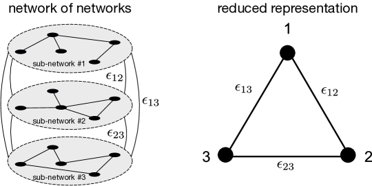
Figure 1: Graphic representation of the system. The network of networks is given by $M$ sub-networks with $N$ nodes each one. Here, we use a two-level system, where each sub-network (area) has internal connections in addition to the inter-area connections. Our approach allows us to study the dynamics of these systems using a reduced $M\times M$ system. This figure depicts an example with $M=3$ sub-networks.

IV.1 Phase synchronization

We first consider a network of networks with $M=3$, where each sub-network is composed of $N=100$ nodes. The internal connection structure of each sub-network is given by random networks. Particularly, we consider Erdős-Rényi matrices with probability given by $0.15$. The adjacency matrix for the internal coupling is given by $A_{ij,\,\text{intra}}=1$ if nodes $i$ and $j$ are connected, and by $A_{ij,\,\text{intra}}=0$ otherwise, while the internal coupling strength is given by $\epsilon_{\mathrm{intra}}=1.0$. The inter-layers coupling scheme is given by a complete graph, where all nodes in one layer are connected to all nodes in another layer with coupling strength that varies randomly between each pair of sub-networks in the interval of $\epsilon_{\mathrm{inter}}\in[0.005,0.01]$.

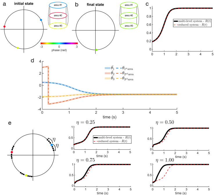
Figure 2: Dynamics on a network of networks and its reduced system with random initial conditions. In the beginning of the simulation, each area is phase synchronized but on different phases (a), therefore the multi-level system is nonsynchronized. (b) As time evolves, due to the inter-area coupling, the internal dynamics changes and the multi-level system transition to phase synchronization. (c) Here, the dynamics of the multi-level system and the reduced one are the same, which is expressed by the Kuramoto order parameter $R(t)$. (d) The trajectories for both the reduced system and the multi-level show that: (i) these systems have equivalent dynamics; and (ii) the network transitions to phase synchrony as time evolves. (e) Our approach can be used even when the oscillators within a sub-network do not have the same phase. We use the broadcast procedure and then apply a perturbation over the phases of the oscillators with amplitude $\eta$. The reduced system and the network of networks have equivalent dynamics even in the presence of this perturbation; however, if the perturbation is too big, our approach no longer can be applied.

The first example is depicted in Fig. 2. Here, the initial state is given by randomly selected phases for each area, which are represented in the unitary circle in color-code (Fig. 2a). All oscillators in each area have the same phase, therefore each sub-network is phase synchronized, but the entire, multi-level system is not – in the beginning of the simulation. As time evolves, the multi-level system transitions to phase synchrony due to the inter-area coupling, which leads all oscillators in all areas to depict the same phase in the final state (Fig. 2b).

The change on the dynamics over time is represented by the Kuramoto order parameter (Fig. 2c), which is evaluated through Eq. (II.11) for the network of networks and through Eq. (II.12) for the reduced system. Here, one can observe that both systems have equivalent dynamics: at $t=0$, $R$ has a low value due to the random phases on the initial state; due to the coupling, $R(t)$ increases as time evolves and, at $t\approx 2$, the order parameter reaches the unity once both systems reach phase synchronization.

In order to show details on the dynamical equivalence between the reduced system and the multi-level network, we plot the trajectories given by the phases of the oscillators in Fig. 2d. Here, the phases in the reduced system are represented by the solid-shaded lines, and the phases of the oscillators in the multi-level network are given by the dashed lines. This result emphasizes that: (i) these systems have equivalent dynamics, and also (ii) the network transitions to phase synchrony as time evolves since the oscillators converge to the same phase.

Furthermore, we can consider the case where the oscillators within each sub-network (area) do not have the same phase at the beginning of the analysis. To do so, we use the same broadcast procedure in addition to a random perturbation with amplitude $\eta$ (Fig. 2e). In this case, the phase of each oscillator within a sub-network is randomly chosen around the phase of this area in the reduced system. Figure 2e shows that the reduced system is able to capture the dynamics of the network of networks even in the presence of perturbation over the initial state. However, if the perturbation is too big, the reduced system and the multi-level network no longer have equivalent dynamics.

IV.2 Unstable twisted states

We use the same system to analyze a different kind of dynamical behavior: phase-locking states, where a constant phase difference is observed across oscillators [37]. This kind of state is also known as “twisted states”, and, for a network with $M$ units, the $p^{\mathrm{th}}$ twisted state is given by:

$$\bm{\theta}^{(p)}=\left(0,\frac{-2\pi p}{M},\cdots,\frac{-2\pi p(M-1)}{M}\right).$$ (IV.1)

We use this equation to obtain the twisted states for the reduced system and then use the broadcasting approach to extend this to the network of networks.

We consider here the same network as in Fig. 2: $3$ sub-networks, where each one is composed of $N=100$ nodes, and the internal connection structure of each area is given by a random network. Here, the internal coupling is given by $\epsilon_{\mathrm{intra}}=1.0$ and the coupling between sub-networks is given by $\epsilon_{\mathrm{inter}}=0.01$. The reduced system is then given by a $3$ nodes network, which is coupled in an all-to-all scheme. A possible phase-locking state for this network, following Eq. (IV.1) is represented in Fig. 3a, where constant difference of $\nicefrac{{2\pi}}{{3}}$ is observed. As stated before, all oscillators within a layer have the same phase, so each area is phase synchronized, but the entire system, in this particular case, has $R=0$, given the phase-locking solution.

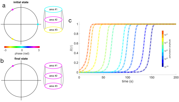
Figure 3: Dynamics on a network of networks and its reduced system on a phase-locking state. (a) We consider a twisted state for the reduced system following Eq. (IV.1) with $M=3$ and $p=1$. This leads to an initial state where a constant phase difference is observed across nodes. (b) However, this twisted state is not stable, so as time evolves, a transition to phase synchrony is observed, and all oscillators have the same phase in the final state. (c) The time at which this transition occurs, however, depends on the perturbation applied to the system. We considered different perturbations amplitudes (color-code) and analyze the Kuramoto order parameter as a function of time for the reduced system (solid-shaded lines) and for the multi-level network (dashed lines). The bigger the perturbation the faster the transition, and our approach shows a perfect match between the dynamics of the reduced system and the multi-level network.

This state, however, is not stable, so small perturbation, e.g. due to the coupling or perturbation on the initial state, can lead the system to transition to phase synchronization (Fig. 3b). Our approach is able to capture the details of this transition. To show this point, we perform a detailed simulation protocol, where different perturbations are applied to the initial state. This perturbation is given by a uniform, random distribution of phases, multiplied by an amplitude factor. Mathematically, the perturbation can be described by: $\mathcal{A}\,\mathcal{U}(-\pi,\pi)$, where $\mathcal{A}$ is the perturbation amplitude. Figure 3c depicts the Kuramoto order parameter as a function of time when different amplitudes are considered, which are represented in color-code. Here, the order parameter for the reduced system is shown in the solid-shaded lines, and the order parameter for the network of networks is shown in the dashed lines. We observe that the smaller the perturbation, the longer it takes for the phase-locking state to transition to phase synchrony. We emphasize that our reduced approach has equivalent dynamics to the multi-level system, so we observe a perfect match.

IV.3 Higher number of sub-networks

The approach introduced here through the reduced system and the broadcasting process is general to study network of networks with an arbitrary number of sub-networks and internal connection scheme. To show this point, we then analyze a multi-level system composed of $M=50$ sub-networks, where each one is given by a random network with $N=100$ nodes. Here, all sub-networks are connected, such that the reduced system is given by a complete graph with $M=50$ nodes, and the internal coupling strength is given by $\epsilon_{\mathrm{intra}}=1.0$ and inter-areas coupling varies in different simulations $\epsilon_{\mathrm{inter}}\in[0.001,0.005]$.

At first, we consider the case of random initial conditions for the reduced system and use the broadcast mechanism to obtain the initial conditions for the multi-level network. Figure 4a show the trajectories for the reduced (solid-shaded lines) and the multi-level systems (dashed lines) based on the phases of the oscillators ($\bar{\theta}$ and $\theta$). Due to the random initial conditions (see the inner panel for the initial state), the systems are desynchronized in the beginning of the simulation. However, as time evolves, phase synchronization is reached and all oscillators have the same phase (see inner panel for final state). This result also shows the equivalence in the dynamical behavior of both systems.

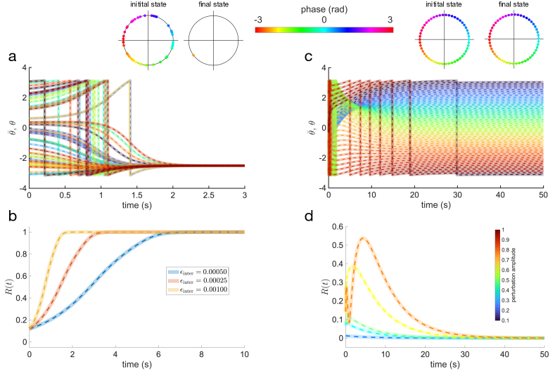
Figure 4: Dynamics on a network with $50$ sub-networks and its reduced system. We first consider the case where the inter-area coupling scheme is given by a complete graph (all-to-all). So, random initial conditions evolve to phase synchrony. Here, solid-shaded lines represent the reduced system, and dashed lines represent the network of networks. The trajectories of the systems emphasize this point (a) and also show the equivalent dynamics between the systems. When we consider higher coupling strengths, the systems transition to phase synchrony quicker (b). We then consider the case where the inter-area connection scheme is given by a first-neighborhood architecture, where each area is connected to two areas (one in each direction) with periodic boundary conditions. In this case, phase-locking solutions are stable. We then show that the systems assume the form of a twisted state (c); and that this is robust to different perturbations (d).

Moreover, if we consider different coupling strengths between the sub-networks (inter coupling), the transition to phase synchrony occurs at different times, as described in Prop. (II.1). To show that our approach is able to capture these details, we consider the same random initial conditions and we change the inter coupling strength. Figure 4b shows the order parameter for the reduced system (solid-shaded lines) and for the equivalent network of networks (dashed lines) as a function of time for different values of $\epsilon_{\mathrm{inter}}$. We observe that the higher the coupling the faster the transition to phase synchronization. Further, this follows from Prop. II.1, and, in addition to that, we are able to quantify to what extent the increase on the coupling $\epsilon_{\mathrm{inter}}$ reduces the time to reach phase synchronization, given by $R(t)=1$.

We also use the approach introduced in this paper to analyze the broadcasting of stable phase-locking states. To do so, we consider the multi-level system with $M=50$ sub-networks, each one being described by a random network with $N=100$ nodes. Each sub-network, however, is connected to two sub-networks only, in a first-neighborhood fashion. This leads to a reduced system being described as a ring graph with $N=50$ nodes, where each node has degree $2$ with periodic boundary conditions. This kind of network is known to support stable twisted states [37]. Particularly, we use Eq. (IV.1) with $M=50$ and $p=1$ to generate the stable phase-locking solution [37] for the reduced system, which is broadcasted to the network of networks following the approach described in this paper. Moreover, to show the stability of this solution and that our approach is able to capture these details, we apply perturbation to this phase-locking state using the same approach as before introduced: $\mathcal{A}\,\mathcal{U}(-\pi,\pi)$.

The trajectories for both, the reduced system and the network of networks are shown in Fig. 4c. In this case, the initial state is given by a twisted state as shown in the inner panel. We then apply a perturbation to this state, which leads to a change in the phase configuration. However, given the stability of the $1^{\mathrm{st}}$ ($p=1$) twisted state for this system, despite the perturbation, the phase-locking is recovered and we can observe the constant phase difference across the oscillators, which leads to the final state being exactly the same as the initial one without perturbation (Fig. 4c inner panels). Again, the phases for the reduced system are represented by the solid-shaded lines, and the phases for the multi-level networks are represented by the dashed lines.

We also consider different perturbation amplitudes applied to the initial state. Figure 4d shows the Kuramoto order parameter for both systems (solid-shaded lines represent the reduced system and dashed lines the multilayer network) as a function of time. The perturbation amplitude is shown in color-code. We observe that the stronger the amplitude the bigger the variation of the order parameter, but given the stability of this state, in the end, $R=0$ for all cases, which characterizes the solution for these systems.

V Discussions and conclusions

In this paper, we have introduced an alternative approach to study and predict the dynamical behavior of Kuramoto oscillators on a class of networks of networks. Based on the results presented in [21, 22], we can represent these networks as a join of matrices, each one representing a different connection between nodes either in the same sub-network or in different sub-networks. From this representation, we have developed a “reduced system” that holds the important information regarding the original, multi-level network. While the network of networks is composed of $M$ sub-networks with $N$ nodes, the reduced system is given by $M$ elements. We have shown that, when the initial state of the multi-level system has a relation with the initial state of the reduced one, both systems have equivalent dynamics. Thus, it allows us to investigate the dynamical behavior of the network of networks in a simpler way.

This problem has sparked a lot of interest due to its wide range of applications. The idea of finding a reduced, simpler version of a sophisticated system has been explored focusing on different aspects of multi-level networks and dynamics [12, 11, 24, 25, 26, 20, 14, 13]. In our paper, we have explored this problem in order to contribute to this discussion. Our results have shown that we can find solutions for the reduced system and broadcast them to the network of networks. This method offers an alternative and simple way to find equilibrium points for Kuramoto oscillators on these networks. This approach is general to arbitrary topologies for intra-areas connections (within each sub-network). Importantly, we have extended the discussion on multi-level networks and dynamics regarding the stability of a given solution. In our paper, we have shown that we can use the approach we have introduced to obtain information on the linear stability of equilibrium points in multi-level networks. We can write the Jacobian matrix for both systems, the multi-level and the reduced one, and, by using the results from [21], we can obtain the spectrum of the Jacobian of the multi-level network based on the spectrum of the Jacobian of the reduced system. Therefore, we are now able to investigate the linear stability of equilibrium points of network of networks in a simple way.

At the same time that our approach contributes to the discussion of the dynamics in multi-level systems, however, there are several open problems yet to be solved. The approach we have shown in this paper was studied in a simple version of a multi-level system. In this way, the extension of this approach to multilayer networks with different coupling functions and different individual dynamics, and the consideration of different dynamical states than phase synchronization within each sub-network are important features that would contribute to the study of the dynamical behavior of multi-level systems.

This is an important problem in modern science, since these networks have been used to model a variety of systems. Extensive numerical studies have shown a rich repertory of dynamical behavior [50, 51, 52]. Moreover, experimental analyses confirm this feature [53, 54]. Furthermore, the use of multi-level networks has been helpful in the understanding of complex systems, e.g. neural systems [4, 55]. However, analytical treatment for this kind of system is still an open problem in these diverse fields. Our approach thus offers a novel path in the study of multi-level network, opening the possibility of analytical and mechanistic insights into the dynamics of these important systems.

Code availability

An open-source code repository for this work is available on GitHub: mullerlab.github.io.