Automatically Score Tissue Images Like a Pathologist by Transfer Learning

Abstract

Cancer is the second leading cause of death in the world. Diagnosing cancer early on can save many lives. Pathologists have to look at tissue microarray (TMA) images manually to identify tumors, which can be time-consuming, inconsistent and subjective. Existing automatic algorithms either have not achieved the accuracy level of a pathologist or require substantial human involvements. A major challenge is that TMA images with different shapes, sizes, and locations can have the same score. Learning staining patterns in TMA images requires a huge number of images, which are severely limited due to privacy and regulation concerns in medical organizations. TMA images from different cancer types may share certain common characteristics, but combining them directly harms the accuracy due to heterogeneity in their staining patterns. Transfer learning is an emerging learning paradigm that allows borrowing strength from similar problems. However, existing approaches typically require a large sample from similar learning problems, while TMA images of different cancer types are often available in small sample size and further existing algorithms are limited to transfer learning from one similar problem. We propose a new transfer learning algorithm that could learn from multiple related problems, where each problem has a small sample and can have a substantially different distribution from the original one. The proposed algorithm has made it possible to break the critical accuracy barrier (the 75% accuracy level of pathologists), with a reported accuracy of 75.9% on breast cancer TMA images from the Stanford Tissue Microarray Database. It is supported by recent developments in transfer learning theory and empirical evidence in clustering technology. This will allow pathologists to confidently adopt automatic algorithms in recognizing tumors consistently with a higher accuracy in real time.

Index terms— Tissue image scoring, Transfer learning, Small training sample, Multiple small auxiliary sets

1 Introduction

Cancer continues to affect millions of people, yet many types of cancers, e.g. pancreatic cancer, mesothelioma, gallbladder cancer, brain cancer etc, have very low survival rates. This has left treatments such as surgery, chemotherapy, and radiation therapy as the main options. As early cancer treatment significantly improves survival rates, the need for early diagnosis is imperative. Despite the importance and necessity of early diagnosis, it can take up to weeks before pathology reports are delivered.

The tissue microarray (TMA) is an emerging technology to analyze tissue samples. It uses thin slices of tissue core samples that are arranged in an array format in paraffin blocks [16]. Biomarkers are applied and typically biomarker-specific dark colors of yellow stains are shown when there is presence of tumors. TMA images are then captured with a high-resolution microscope. The scoring of TMA images is based on the severity of tumors, and a common system for scoring TMA images uses a scale from 0 to 3, where a score of 0 indicates no tumors, and a score of 3 implies very severe tumors which corresponds to late stages of cancer progression, for example, Stage IV in a common 4-stage (Stage I, II, III, and IV) cancer grade system. TMA technology makes it possible to efficiently analyze many tissue samples together, thus normalizing conditions for comparative studies. These benefits give TMA images the potential to be widely used as an effective technique for diagnosis and prognosis oncology [20, 25]. A valuable source to explore TMA images is the Stanford TMA image database [23], publicly available from https://tma.im/tma_portal/, and work presented here is based on TMA images from this database.

The diagnosis for tumors—identifying tumors from staining patterns in tissue images—manually is time-consuming and can easily be inconsistent [7, 32]. Although structured procedures have been proposed, manual scoring can still be fairly subjective [33, 4], and the same pathologist may score differently at different sessions for the same image. Because of these issues, a number of algorithms, including ACIS, Ariol, TMALab, AQUA [6] and TACOMA [33], have been developed to automate this process. These algorithms, although transformative, are not widely adopted due to limits in their capabilities. They require substantial involvement of pathologists on tasks such as TMA image background subtraction, feature segmentation, thresholds of hue or pixel intensity, and the provision of representative TMA image patches etc.

The variability of staining patterns in TMA images and the scarcity of training samples make it particularly challenging to develop an automatic algorithm. Staining patterns in TMA images can have very different sizes, locations, shapes, and colors, despite having the same score. Figure 1 demonstrates the variability of staining patterns in the TMA images.

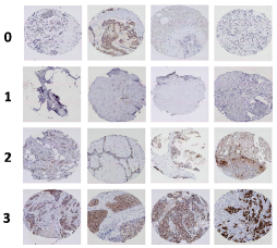
Figure 1: The staining patterns vary highly across TMA images. Images with the same score can look drastically different.

The high variability in the staining patterns also increases the need for larger sample sizes in training algorithms. Having more images would allow the algorithm to capture more variability in the staining patterns, leading to more consistent results. However, the number of TMA images is severely limited due to privacy and regularization concerns in medical organizations. Moreover, the TMA images currently available are for over 100 different types of cancers, with very few numbers of TMA images available for each individual cancer type. In recent years, deep learning [14] has become the method of choice for many image recognition tasks. However, that is not feasible for TMA image scoring due to the small sample size available for a given cancer type.

This work aims to develop an automatic algorithm for the scoring of TMA images at the accuracy level of pathologists by augmenting the training sample with transfer learning [8]. The key observation is that, some of the TMA images of a different cancer type may look similar (i.e., have a similar staining pattern) to those of the given cancer type and with the same score, thus making it possible for transfer learning. However, usual algorithms for transfer learning (many based on deep neural networks [29]) are not applicable since we do not have a large dataset from similar problems as the basis for knowledge transfer—while there exist many different cancer types, the number of TMA images of each individual type is small. This gives rise to a new transfer learning setting: there are multiple similar learning problems around but each has only a small training sample, and we wish to design an algorithm that could effectively transfer knowledge from all the similar learning problems. The approach we take is instance-based transfer learning [8], where we propose to selectively include TMA images of other cancer types with similar staining patterns as the cancer type of interest. With an enlarged training set, we can expect to improve accuracy on the scoring of TMA images of the original cancer type. Given the huge success of transfer learning in application domains such as natural language processing and image recognition, we expect that it would enable the automatic evaluation of cancer tumors in TMA images at the level of pathologists.

The remaining of this paper is organized as follows. In Section 2, we describe our approach and algorithms design. Experiments and results are presented in Section 3, along with a discussion of connections of our algorithm to recent theoretical developments in transfer learning. Finally we conclude in Section 4.

2 Methods

We formulate the scoring of TMA images as a classification problem. Our approach can be summarized as follows. A type of tumor-specific spatial histograms is used to capture key features characterizing the staining patterns in tissue images, then transfer learning is adopted to increase the training sample size by selectively including images of other cancer types. The enlarged training set is input to Random Forests (RF) [2] classifier to re-fit the classification model and results reported. The goal is to achieve or exceed the accuracy level of pathologists. A detailed description about spatial histogram, RF, transfer learning, and the algorithmic implementation of our approach will be presented in Sections 2.1, 2.2, 2.3, and 2.4, respectively.

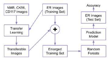
Figure 2: Illustration of the overall flow of the proposed algorithm. The ’+’ sign stands for combining images from multiple sources. ER is the name of biomarker associated with the target cancer type and we use it to indicate the corresponding TMA images, while NMB, CK56 and CD117 are those for other cancer types.

Figure 2 shows the overall flow of our approach. Note that here for illustration purpose, we use ‘ER’, the name of a biomarker for breast cancer, to indicate the cancer type of interest, while using ’NMB’, ‘CK56’, or ‘CD117’ for other cancer types. One major challenge in the automatic scoring of TMA images is the variability in the staining patterns, which may have different shapes, sizes, and locations despite having the same score. The staining patterns are encoded by spatial histograms, following work in [33]. The spatial histogram also helps to greatly reduce the data dimensionality, another challenge in the automatic scoring of TMA images which is caused by large image sizes (i.e., $1504\times 1410$). RF is used as the classifier for its strong built-in feature selection capability. To implement transfer learning, our main effort lies in evaluating whether an image of other cancer types is conformal to the hypothesis (or decision rule) induced by images of the original cancer type.

2.1 The spatial histogram

The staining patterns on TMA images can vary highly, even for those with the same score. Thus, it is desirable to look for image features that are relatively stable across images of the same score. The feature we use is a spatial histogram matrix (or gray level cooccurrence matrix in the remote sensing literature [17]), which is commonly used for textured images. It is a suitable image feature because TMA images belong to one of the two major classes of textured images—images taken from very far away in the sky (for example, remote sensing images) and those taken under a high resolution microscope. Indeed, the spatial histogram has been used in literature for TMA images [33] and fares well.

Similar to the conventional histogram, the spatial histogram is a collection of counting statistics about pairs of adjacent (or neighboring) pixels in an image and represented as a matrix.

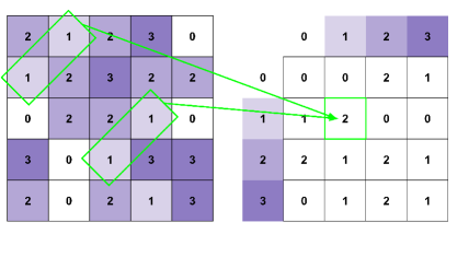
Figure 3: Illustration of a toy image and the spatial histogram matrix. The left panel stands for the original image where the numbers are the gray values, and the right is the resulting spatial histogram matrix with a dimension $4\times 4$. The two diagonally (i.e., along 45 °direction) neighboring pixels with both gray levels of 1 occur twice in the image, so the (1, 1)-entry of the spatial histogram matrix has a value of 2.

In generating a spatial histogram, we only consider neighboring pixels that have a predefined spatial relationship. That is, the two pixels need to have a pair of given pixel values and are neighbors along a certain direction. A typical choice for the direction is the $45\degree$ direction in the image grid. Figure 3 shows an example of such neighboring pixels where the pairs of pixels of interest are marked by green rectangles and both have grey value 1. The counting statistic is the total number of times such a pair occur in the image grid along the $45\degree$ direction, and this gives the value of the (1,1)-entry of the spatial histogram matrix. Similarly, pairs of pixels along the same direction but with pixel values $i$ and $j$, respectively, would produce a counting statistic for the (i,j)-entry of the matrix, and so on.

One can choose to use a different spatial relationship, like pairs along a direction of $0\degree$ or $135\degree$ etc in the image grid, and the difference in TMA image scoring would be small. Also, one can extend the distance between the neighboring pixels. The default distance is 1, indicating immediate neighbors. The two pairs of example pixels in Figure 3 all have a distance 1, while a distance of 2 or larger would indicate a larger staining pattern. In this work, a spatial distance of 2 is used.

One nice feature about the use of spatial histogram is dimension reduction. The TMA images are large in size, and those from the Stanford TMA image database [23] have a size of $1504\times 1440$. Directly working with such images would require enormous computing power and memory, and worse still, that will lead to the curse of dimensionality, as each image would be treated as a huge vector of a dimension more than 2 million (i.e., $1504\times 1440$). As the gray value of TMA image pixels have a range between 0 and 255, the spatial histogram will reduce the data dimension to a value, $256\times 256$, much smaller than that from the original image. One step further is to apply a quantization to the image gray values. That will lead to an even smaller spatial histogram matrix. We follow work in [33], and apply a linear quantization to the gray values into 51 levels. That is, a gray value of $5\cdot x+y$ for $0\leq x\leq 50$ and $0\leq y\leq 4$ will be transformed to $x+1$ (255 is converted to 51 for simplicity). Thus the spatial histogram matrix now has a dimension of $51\times 51$, and a vector (of dimension 2601) formed by collapsing this matrix is used as input to the RF classifier so that computation can be done very efficiently. Importantly, this also makes the resulting image features stable against small variations in image pixel values due to varying physical conditions such as lighting or illumination.

2.2 Random Forests

RF is used as the classification engine for our TMA image scoring algorithm. RF is an ensemble of decision trees, and each tree is grown by recursively splitting the data. At each node split, RF randomly samples a number of features (called number of tries) and selects one leading to their best partition of that node, according to some criterion. Each tree progressively narrows down the decision for an instance. The node split continues until there is only one point in the node (for classification) or when the node is pure (i.e., all the points in the node have the same label). At classification, an instance receives a vote on its class label from each tree in RF, and the final decision given by RF is a majority vote on the class labels, according to the number of votes that each label gets from all trees.

Many studies have reported excellent performances of RF [2, 9]. For TMA image classification, previous studies [19, 33] also show that RF outperforms competitors like SVM [10] or boosting [13]. Compared to its competitors, RF scales well against some main challenges in TMA image scoring, including high dimensionality and label noise, thanks to its strong feature selection ability and ensemble nature. RF is easy to use with very few tuning parameters—often one just need to set the number of trees and the number of tries at each node split.

2.3 Transfer learning

Transfer learning [8] is an emerging learning paradigm to address the problem of insufficient training data when there is a large set of auxiliary data (called auxiliary set) that entails knowledge helpful in solving the original problem. Transfer learning algorithms can be classified as instanced-based, mapping-based, representation-based, or feature-based transfer learning [29]. Instance-based transfer learning [11] transfers knowledge in the form of enlarging the original training set by finding instances in the auxiliary set that are consistent with the hypothesis learned on the original training set (such instances are called transferable). Mapping-based transfer learning [31] learns semantically sensible invariant representation across the original and auxiliary sets. Feature-based approaches [22] learn features that would help the learning of the original problem. Representation-based [15, 24] tries to find representations that can be transferred. Recently, deep transfer learning [14] has become very popular and achieves impressive performance in a number of domains, for example, large natural language processing systems such as BERT [12] and GPT-3 [3], and pre-trained image models [30]. The literature on transfer learning is enormous, and we can only mention a few here. More discussion can be seen in [26, 29, 1] and references therein.

The lack of a large auxiliary dataset makes transfer learning particularly challenging for the problem of TMA image scoring. The big family of deep neural networks based transfer learning algorithms are not applicable here due to the reliance on the training of large deep networks, which inevitably requires a huge training set. In the scoring of TMA images, there are multiple auxiliary sets available as images from a number of other cancer types can look very similar to those of the cancer type of interest. However, none of the auxiliary sets is large enough for the typical deep neural networks based approaches to be feasible. Thus, we now have a new problem setting for transfer learning, and we wish to enable knowledge transfer from multiple small auxiliary sets.

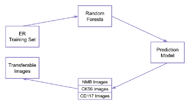
Figure 4: Illustration of transfer learning. ER is the name of biomarker associated with the target cancer type, while NMB, CK56 and CD117 are those for other cancer types.

The approach we take is instance-based transfer learning, and Figure 4 is an illustration of the algorithm. We first fit a prediction model (called original hypothesis) using RF on the original training set. Then from the auxiliary set, we try to identify TMA images that are consistent with the original hypothesis. Clearly we do not require a large auxiliary set to achieve this. We can add those transferable images to enlarge the original training set. For a small training set, increasing its size will likely improve performance on the test set. In Figure 5, the left 3 columns show example images for the target cancer type—breast cancer (indicated by ER) where each row corresponds to a different score. The right columns are example images from a different cancer type (marked by NMB, CK56 and CD117, respectively) that look similar (to certain extent) to the breast cancer images with the same score.

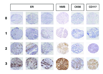
Figure 5: Example transferable images from other cancer types. The left 3 columns of images are TMA images for breast cancer and indicated by the associated biomarker estrigen receptor (ER). The right 3 columns are TMA images for cancer types indicated by biomarkers NMB, CK56 and CD117, respectively, which have a similar appearance as those for ER with the same label.

2.4 An algorithmic description

In our algorithm, transfer learning is implemented as function, $tmaTransfer()$, which finds transferable images from a given auxiliary set. The main function, $tmaScore()$, calls $tmaTransfer()$ to obtain transferable images from other cancer types, fits model on the enlarged training set via RF, and then reports final results on the test set.

$tmaTransfer()$ is implemented as follows. We first fit a classification model, $\mathbb{M}_{0}$, by RF on the original training set $\mathcal{T}_{0}$. Then we apply $\mathbb{M}_{0}$ to the set of auxiliary images, $\mathcal{W}$. If the predicted label for an image, $W\in\mathcal{W}$, is the same as its given label (note the label for these images in the auxiliary set are known since they come with the TMA images in the Stanford database), then we say image $W$ (along with its label) is consistent with the original model hypothesis $\mathbb{M}_{0}$. As there might be label noise for image $W$, we only transfer images that are predicted more confidently. The confidence in prediction can be estimated from the number of votes $W$ receives on different class labels (or scores) from trees in RF. If the majority class gets substantially more votes than other classes, then we say the instance is predicted with high confidence. Here, the majority class is the one that receives the most votes. An easy way to estimate the confidence is to use the difference in the fraction of votes received for the top and the second majority class (the class that receives the second most number of votes). Let $n_{1}(W)$ and $n_{2}(W)$ be number of votes $W$ gets on the top and second majority class, and $T$ be the number of trees in RF. We can estimate the confidence in predicting instance $W$ as follows

$$\beta(W)=\frac{n_{1}(W)-n_{2}(W)}{T}.$$ (1)

So $\beta(W)$ has a value in the range $[0,1]$, and a TMA image $W$ in the auxiliary set is selected if it is classified with a confidence larger than a predetermined level $\beta_{0}$. The choice of $\beta_{0}$ seeks to include TMA image instances that are valuable to the original problem. Singh and his coauthors [28] study the contribution of individual data points to algorithmic performance in semi-supervised classification problem, and they find that data points that are along the decision boundary barely help, while the value of a data point increases when the data point is slightly away from the boundary. Our definition of confidence aims to avoid data points that are along or very close to the decision boundary (such data points would be classified with very low confidence), while trying to include data points that are slightly away from the decision boundary. Note that a too big value of $\beta_{0}$ is not desirable either, as that will cause the inclusion of only data points far away from the decision boundary. Let $\mathcal{F}$ denote the transferable set (which is the set of images transferred from the auxiliary sets). The $tmaTransfer()$ function is implemented as Algorithm 1.

Algorithm 1   tmaTransfer($\mathbb{M}_{0},\mathcal{W},T,\beta_{0}$)

1:  Initialize the transferable set $\mathcal{F}\leftarrow\emptyset$;

2:  while $\mathcal{W}$ is not empty do

3:     Pick an image $W$ from $\mathcal{W}$, and set $\mathcal{W}\leftarrow\mathcal{W}\setminus\{W\}$;

4:     Apply the original model $\mathbb{M}_{0}$ to $W$;

5:     if predicted label on $W$ is different from its given label then

6:        Skip to the next round of the loop;

7:     end if

8:     Calculate the prediction confidence $\beta(W)$ for image $W$;

9:     if $\beta(W)\geq\beta_{0}$ then

10:        Add $W$ to the transferable set, $\mathcal{F}\leftarrow\mathcal{F}\cup\{W\}$;

11:     end if

12:  end while

13:  return($\mathcal{F}$);

To describe algorithm for the main function $tmaScore()$, assume that the other cancer types for transfer learning are associated with biomarkers NMB, CK56 and CD117 for simplicity of description. Let the set of auxiliary images for these cancer types be denoted by $\mathcal{W}_{nmb},\mathcal{W}_{ck56},\mathcal{W}_{cd117}$, respectively. Function $tmaScore()$ first fits a prediction model, $\mathbb{M}_{0}$, from the original training set using RF. Then, it identifies the transferable set from each auxiliary set in $\{\mathcal{W}_{nmb},\mathcal{W}_{ck56},\mathcal{W}_{cd117}\}$. Add the transferable set to the original training set $\mathcal{T}_{0}$, re-fit the prediction model, then apply it to the test set and report results. The main function is implemented as Algorithm 2.

Algorithm 2   tmaScore()

1:  Let the number of trees in Random Forests be $T$;

2:  Apply RF to the original training set $\mathcal{T}_{0}$;

3:  Let the fitted Random Forests model be $\mathbb{M}_{0}$;

4:  Pick a predefined confidence level $\beta_{0}$;

5:  Initialize the transferable set $\mathcal{F}\leftarrow\emptyset$;

6:  for $\mathcal{W}$ in $\{\mathcal{W}_{nmb},\mathcal{W}_{ck56},\mathcal{W}_{cd117}\}$ do

7:     Apply transfer learning to image set $\mathcal{W}$;

8:     $\mathcal{F}_{t}\leftarrow tmaTransfer(\mathbb{M}_{0},\mathcal{W},T,\beta_{0})$;

9:     Add $\mathcal{F}_{t}$ to the transfer set $\mathcal{F}\leftarrow\mathcal{F}\cup\mathcal{F}_{t}$;

10:  end for

11:  Add transferable set $\mathcal{F}$ to original training set $\mathcal{T}_{0}$ and re-fit RF;

12:  Apply the re-fitted model to test set $T_{s}$ and report accuracy;

3 Experiments and results

We conduct experiments using TMA images from the Stanford TMA image database. The cancer type we choose to work with is breast cancer, due to the fact that it is one of the best understood cancer types to date. The associated biomarker is estrogen receptor (ER). There are 690 images in total for ER in the database, and the training and testing sets are randomly split evenly. The reported results are averaged over 100 runs.

TMA images in the Stanford TMA database are from several dozens of different cancer types. One can use TMA images from all other different cancer types, but we take a more conservative approach. Transfer learning requires the auxiliary set to be consistent to hypothesis entailed by the original training set. We browse through the Stanford TMA image database, and determine that TMA images associated with biomarkers NMB, CK56, and CD117 are visually, to a certain extent, similar to TMA images for ER. Note that the actual set of images that can be used as auxiliary set, or images that are transferable, are broader that those visually similar images. In other words, some of the transferable images may not look so “similar” to images in the original training set. Part of our goal in using the term ‘visually similar images’ is for the purpose of describing our motivation with transfer learning.

We use the R package randomForest for our experiments. The number of tries at each node split is chosen among $\{\sqrt{p},2\sqrt{p}\}$, where $p$ is the input data dimension. For TMA images as we work on the spatial histogram matrix, we have $p=51\cdot 51=2601$. The number of trees in RF is fixed at $T=100$, adopting the value used in [33]; indeed we find the difference in results small when varying over a range of choices $\{50,100,200,500\}$. The confidence level $\beta_{0}$ for instance transfer is picked as 10%, implying that only instances with the top majority class leading the second majority class by at least 10% votes (out of $T=100$ trees) are considered to be transferable.

3.1 Results

The evaluation metric is the test set accuracy, which is the percent of test images with a predicted class label agreeing with the given one (that is, the label comes with the database). The results are shown in Figure 6. The accuracy achieved with transfer learning over auxiliary sets associated with NMB, CK56 and CD117 is 75.9%, outperforming the algorithm without transfer learning (shown as the first bar in the figure). The accuracy of pathologists is estimated to be around 75-84% [33], so transfer learning allows our algorithm to achieve the accuracy level of pathologists. It should be noted that the gold standard of comparison vs pathologists in this case would be through consensus scores produced by a group of well-trained pathologists. However, in the lack of consensus pathologists’ scores, estimation by [33] could be viewed as giving the accuracy level of pathologists (on the ER images). It is interesting to see that the achieved accuracy increases progressively when we apply transfer learning over more auxiliary sets, e.g., in the order of over $\mathcal{W}_{nmb}$ only, over two auxiliary sets $\{\mathcal{W}_{nmb},\mathcal{W}_{ck56}\}$, and over three auxiliary sets $\{\mathcal{W}_{nmb},\mathcal{W}_{ck56},\mathcal{W}_{cd117}\}$. Note that comparison with other popular classifiers such as support vector machines and boosting with the spatial histogram matrices as inputs was made previously in [33] for which an accuracy at 65.24% and 61.28% were reported, respectively. The reason why SVM and boosting substantially underperformed is possibly due to the fact that these two classifiers are not able to handle high dimensional and possibly noisy (in labels) inputs well, while RF has strong built-in ability in feature selection with high dimensional inputs and is also remarkably resistant to label noises.

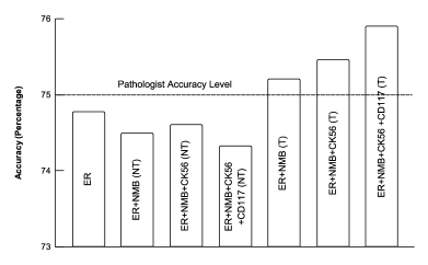
Figure 6: Comparison of accuracy. ’T’ and ’NT’ stand for transfer learning and without transfer learning, respectively, and ER, NMB, CK56, and CD117 indicate the TMA images associated with respective biomarkers.

We also conduct experiments by simply combining the training set of TMA images for ER with images in auxiliary sets $\mathcal{T}_{NMB}$, $\mathcal{T}_{CK56}$ and $\mathcal{T}_{CD117}$. This actually leads to a decrease in accuracy compared to that without transfer learning, as shown in the second thru the fourth bars in Figure 6. Although directly combining data from the auxiliary sets greatly increases the size of the training set, it also makes the data a lot more heterogeneous thus more challenging for classification as we now have to accommodate images of sub-models within the same class label. In comparison, transfer learning with our approach over images from other cancer types, even with different distributions, allows to improve the accuracy if we can properly control the confidence level.

3.2 Understanding the transfer learning scheme

We adopt instance-based transfer learning, and the particular scheme we propose improves the accuracy of TMA image classification. Our algorithm could be understood from recent theoretical developments in transfer learning, and is also empirically supported by experiments.

Transfer learning typically requires similarity in the distribution between the original and the auxiliary set. Recent work towards understanding of transfer learning focuses mainly on relaxing this ideal condition along two lines. One is the covariate-shift model where the marginal distribution of the original and the auxiliary data are different but their induced decision rules (or hypothesis) are similar. Here the marginal distribution refers to the probability distribution of the TMA images or their spatial histograms, while the induced decision rule is the rule that decides which class label (score) a TMA image gets given the pixel values or the spatial histogram of an image. Kpotufe and Martinet [21] study, under the covariate-shift model, how much the target performance is impacted by sample size and the difference in the original and the auxiliary distribution. The other is the posterior-drift model where the marginal distribution of the original and the auxiliary data are similar but their induced decision rules could be very different. Cai and Wei [5] study how fast the estimated decision rule converges to its limit in terms of the difference in the induced decision rules between the target and auxiliary data. For the scoring of TMA images, clearly the distribution of the original and the auxiliary data are different, and so are the induced decision rules. Our approach can be viewed as trying to satisfy the assumption of the covariate-shift model, i.e., it tries to find a subset of the auxiliary data such that the induced decision rule agrees to that from the original data. This is achieved by searching from the auxiliary set those TMA images with the same label as the predicted one under the decision rule learned from the original data (i.e., conformal to the original hypothesis). This effectively overcomes the difficulty in requiring a similar induced decision rule between the original and the entire auxiliary data. Thus, our approach gives a solution to the challenging problem of enabling knowledge transfer from multiple small auxiliary sets with each inducing a potentially different decision rule from that on the original data.

Next, we conduct some experiments. We first produce a visualization of the original training set (corresponding to breast cancer) and that enhanced by transfer learning from other cancer types, including those associated with NMB, CK56 and CD117. Each image in the training set can be viewed as a point in the high dimensional space, and the points are plotted along the first and second component from a principal component analysis [18] of the data. From Figure 7, it can be seen that for the enhanced training set, the separation of points become larger.

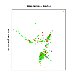
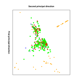
Figure 7: The original and transfer learning enlarged training set visualized by their first and second principal directions via principal component analysis. The top panel is for the original training set, and the bottom panel is for training set enhanced by transfer learning. Different colors correspond to TMA images with a different class label (or score).

In particular, points with color orange now becomes visible (previously they are mostly hiding among points with other colors or labels); some blue points are also better separated from the green and red point clouds. A better separation between classes would make the classification task easier, thus a better accuracy can be expected. Indeed, we can get a more precise characterization of the amount of class separation by the class separation ratio

$$\rho=\sum_{\text{All pairs of classes i, j}}(SSW_{i}+SSW_{j})/SSB_{i,j},$$ (2)

which is the ratio of the within-class sum of squared distances out of the between-class sum of squared distances calculated over all pairs of classes, and $SSW_{i}$ and $SSB_{i,j}$ are defined as

$$SSW_{i} = \sum_{\text{$a,b$ all with label $i$}}distance^{2}(a,b)$$

$$SSB_{i,j} = \sum_{\text{$a$ with label $i$, $b$ with label $j$}}distance^{2}(a,b),$$

where $distance(a,b)$ is the Euclidean distance between points $a$ and $b$. The class separation ratio $\rho$ measures the quality of clustering, so it gives hint on the difficulty in separating different classes. A smaller value of $\rho$ indicates that the within-class distances is small relative to the between-class distance, thus a better separation of classes. The mean class separation ratio is calculated as 15.6668 and 12.1379, averaged over 100 runs on the original and transfer learning enhanced training sets, respectively. This implies that, for the enlarged training set, different classes are better separated. This is consistent with our visualization and experimental results, thus giving empirical support to the transfer learning scheme we propose. Further experiments are expected to better understand this, which we leave for future work.

4 Conclusions

An algorithm has been proposed for the scoring of TMA images via transfer learning. By selectively including TMA images with similar staining patterns from other cancer types, the algorithm is able to achieve the accuracy level of a pathologist. This algorithm is fully automatic and without involvements from the pathologists. One desirable feature of the proposed algorithm is that as more transferable cancer types are considered, the accuracy is improved further. It is interesting to note that the accuracy would suffer if we simply combine TMA images from other cancer types without transfer learning. With this algorithm, pathologists are expected to diagnose cancer patients faster, more accurately, and consistently. Survival rates can be significantly improved because diagnoses can now be made in real-time and patients can be treated earlier.

It is worthwhile to note that we implement transfer learning in a nonstandard setting—the auxiliary set is small and there are potentially multiple auxiliary sets available. It is challenging as typical algorithms for transfer learning are no longer applicable here, and also we wish to enable knowledge transfer from as many auxiliary sets as possible. Our algorithm has sound theoretical support from recent developments in transfer learning. It can be understood as trying to carve out a portion of the auxiliary set so that the covariate-shift model applies, i.e., the selected subset from the auxiliary set is conformal to the original hypothesis.

Empirically, experiments have also been carried out to understand the algorithm. Data visualization shows that our algorithm increases the class separation, and a larger class separation often makes the classification problem easier and thus improved accuracy can be expected. This is corroborated by the empirical class (cluster) separation ratio, which measures the cluster quality, and the enhanced training set leads to a better class separation. One possibility of future work is to explore how to exclude unnecessary parts (or patterns) in TMA images or finding the most important features about TMA images to further increase the accuracy. Additionally, different notions of confidence may be explored for instance transfer, for example those using the concept of conformal classification [27].

5 Acknowledgments

I would like to thank my science research teacher, Mrs. Piscitelli, and Dr. Gordon Wu for their help and advice in the project. I am grateful to the editor, the associate editor, and the anonymous reviewers for their constructive comments and suggestions.

References

- [1] N. Agarwal, A. Sondhi, K. Chopra, and G. Singh. Transfer learning: Survey and classification. In Smart Innovations in Communication and Computational Sciences, pages 145–155, 2021.
- [2] L. Breiman. Random Forests. Machine Learning, 45(1):5–32, 2001.
- [3] T. Brown, B. Mann, N. Ryder, M. Subbiah, and J. Kaplan et al. Language models are few-shot learners. In Advances in Neural Information Processing Systems (NeurIPS), 2020.
- [4] T. Brunye, E. Mercan, D. L. Weaver, and J. G. Elmore. Accuracy is in the eyes of the pathologist: The visual interpretive process and diagnostic accuracy with digital whole slide images. Journal of Biomedical Informatics, 66:171–179, 2017.
- [5] T. Cai and H. Wei. Transfer learning for nonparametric classification: Minimax rate and adaptive classifier. The Annals of Statistics, 49(1):100-128, 2021.
- [6] R. Camp, G. Chung, D. Rimm, et al. Automated subcellular localization and quantification of protein expression in tissue microarrays. Nature medicine, 8(11):1323–1327, 2002.
- [7] R. Camp, V. Neumeister, and D. Rimm. A decade of tissue microarrays: progress in the discovery and validation of cancer biomarkers. Journal of Clinical Oncology, 26(34):5630–5637, 2008.
- [8] R. Caruana. Multitask learning. Machine Learning, 28:41–75, 1997.
- [9] R. Caruana, N. Karampatziakis, and A. Yessenalina. An empirical evaluation of supervised learning in high dimensions. In Proceedings of ICML, pages 96–103, 2008.
- [10] C. Cortes and V. N. Vapnik. Support-vector networks. Machine Learning, 20(3):273–297, 1995.
- [11] W. Dai, Q. Yang, G. Xue, and Y. Yu. Boosting for transfer learning. In Proceedings of the 24th International Conference on Machine Learning (ICML), 2007.
- [12] J. Devlin, M.-W. Lee, and K. Toutanova. Bert: Pre-training of deep bidirectional transformers for language understanding. In Proceedings of the Conference of the North American Chapter of the Association for Computational Linguistics: Human Language Technologies, 2019.
- [13] Y. Freund and R. Schapire. Experiments with a new boosting algorithm. In Proceedings of the 13rd International Conference on Machine Learning (ICML), 1996.
- [14] I. Goodfellow, Y. Bengio, and A. Courville. Deep Learning. The MIT Press, 2016.
- [15] I. Goodfellow, J. Pouget-Abadie, M. Mirza, B. Xu, D. Warde-Farley, S. Ozair, A. Courville, and Y. Bengio. Generative adversarial nets. In Advances in Neural Information Processing Systems (NIPS), 2014.
- [16] W. Grace-Jones. Tissue microarray. Theory and Practice of Histological Techniques (6th Edition), pages 527–535, 2012.
- [17] R. M. Haralick. Statistical and structural approaches to texture. Proceedings of IEEE, 67(5):786–803, 1979.
- [18] T. Hastie, R. Tibshirani, and J. Friedman. The Elements of Statistical Learning: Data Mining, Inference, and Prediction. Springer, 2001.
- [19] S. Holmes, A. Kapelner, and P. Lee. An interactive Java statistical image segmentation system: Gemident. Journal of Statistical Software, 30(10):1–20, 2009.
- [20] N. Jawhar. Tissue microarray: A rapidly evolving diagnostic and research tool. Annals of Saudi Medicine, 29(2):123–127, 2009.
- [21] S. Kpotufe and G. Martinet. Marginal singularity and the benefits of labels in covariate-shift. The Annals of Statistics, 49(6):3299-3323, 2021.
- [22] M. Long, Y. Cao, J. Wang, and M. Jordan. Learning transferable features with deep adaptation networks. In Proceedings of ICML, 2015.
- [23] R. Marinelli, K. Montgomery, C. Liu, N. Shah, W. Prapong, M. Nitzberg, Z. Zachariah, G. Sherlock, Y. Natkunam, R. West, et al. The Stanford tissue microarray database. Nucleic Acids Research, 36:D871–877, 2007.
- [24] M. Oquab, L. Bottou, I. Laptev, and J. Sivic. Learning and transferring mid-level image representations using convolutional neural network. In Proceedings of the 2014 IEEE Conference on Computer Vision and Pattern Recognition (CVPR), pages 1717–1724, 2014.
- [25] C. Page, A. Mes-Masson, and A. M. Magliocco. Tissue microarrays in studying gynecological cancers. Cancer Genomics, pages 65–76, 2014.
- [26] S. Pan and Q. Yang. A survey on transfer learning. IEEE Transaction on Knowledge and Data Engineering, 22(10):1345–1359, 2010.
- [27] G. Shafer and V. Vovk. A tutorial on conformal prediction. Journal of Machine Learning Research, 9:371–421, 2008.
- [28] A. Singh, R. Nowak and X. Zhu. Unlabeled data: Now it helps, now it doesn’t. In Proceedings of Neural Information Processing Systems (NeurIPS), 21:1513-1520, 2009.
- [29] C. Tan, F. Sun, T. Kong, W. Zhang, C. Yang, and C. Liu. A survey on deep transfer learning. In Proceedings of 27th International Conference on Artificial Neural Networks (ICANN), 2018.
- [30] C. Tan, F. Sun, T. Kong, W. Zhang, C. Yang, and C. Liu. Adversarially robust transfer learning. In International Conference on Learning Representations (ICLR), 2020.
- [31] E. Tzeng, J. Hoffman, N. Zhang, K. Saenko, and T. Darrell. Deep domain confusion: Maximizing for domain invariance. arXiv:1412.3474, 2014.
- [32] H. Vrolijk, W. Sloos, W. Mesker, P. Franken, R. Fodde, H. Morreau, and H. Tanke. Automated acquisition of stained tissue microarrays for high throughput evaluation of molecular targets. Journal of Molecular Diagnostics, 5(3):160–167, 2003.
- [33] D. Yang, P. Wang, B. S. Knudsen, M. Linden, and T. W. Randolph. Statistical methods for tissue microarray images–algorithmic scoring and co-training. The Annals of Applied Statistics, 6(3):1280–1305, 2012.