Testing Bayesian reconstruction methods from peculiar velocities

Abstract

Reconstructing the large scale density and velocity fields from surveys of galaxy distances, is a major challenge for cosmography. The data is very noisy and sparse. Estimated distances, and thereby peculiar velocities, are strongly affected by the Malmquist-like lognormal bias. Two algorithms have been recently introduced to perform reconstructions from such data: the Bias Gaussian correction coupled with the Wiener filter (BGc/WF) and the Hamlet implementation of the Hamiltonian Monte Carlo forward modelling. The two methods are tested here against mock catalogs that mimic the Cosmicflows-3 data. Specifically the reconstructed cosmography and moments of the velocity field (monopole, dipole) are examined. A comparison is made to the “exact” wiener filter as well - namely the Wiener Filter in the unrealistic case of zero observational errors. This is to understand the limits of the WF method. The following is found. In the nearby regime ($d\lesssim 40\,h^{-1}\,{\rm Mpc}$) the two methods perform roughly equally well. Hamlet does slightly better in the intermediate regime ($40\lesssim d\lesssim 120\,h^{-1}\,{\rm Mpc}$). The main differences between the two appear in the most distant regime ($d\gtrsim 120\,h^{-1}\,{\rm Mpc}$), close to the edge of the data. Hamlet outperforms the BGc/WF in terms of better and tighter correlations, yet close to the edge of the data Hamlet yields a slightly biased reconstruction. Such biases are missing from the BGc/WF reconstruction. In sum, both methods perform well and create reliable reconstructions with significant differences apparent when details are examined.

1 Introduction

Figure 1: The distance, in units of km/s, of the CF3 data points (magenta) and mock data points (green) projected on the three supergalactic principal planes. Note the ZOA is accurately reproduced in the mock catalogues.

Figure 2: From left to right, the distribution SGB, SGL and $z$. Note that in panels a and b the two curves are on top of one an other.

Mapping the large scale distribution of matter and its corresponding three-dimensional (3D) velocity field is of great interest. The motivation is threefold. For one, mankind at large, and astronomers in particular, explore their Universe by charting it. Making maps is a first step towards understanding ones surroundings and ones place within a greater environment. Mapping the large scale distribution of matter in the Universe is thus an end unto itself. Furthermore, explaining the large scale velocity and density fields within the context of the $\Lambda$CDM paradigm of structure formation allows for the estimation of cosmological parameters that are inherent to that model (Jaffe & Kaiser, 1995; Pike & Hudson, 2005; Feldman et al., 2010; Nusser & Davis, 2011; Carrick et al., 2015; Qin et al., 2019; Dupuy et al., 2019; Lilow & Nusser, 2021; Boruah et al., 2021b). A third motivation is to map these fields at high redshift, thereby allowing for the reconstruction of the initial conditions of the Local Universe (Yepes et al., 2009; Sorce et al., 2016; Hoffman et al., 2018; Libeskind et al., 2020; Sawala et al., 2021).

We focus here on mapping the large scale structure (LSS) of the universe from surveys of peculiar velocities, or rather from surveys of galaxies with measured distances from which the radial component of the peculiar velocities may be extracted. Measuring galaxy distances is a formidable challenge in observational cosmology. All distance measures rely on comparing an observed magnitude with an (inferred or assumed) absolute magnitude. There are many ways to estimate a galaxy’s distance. For example, scaling relations tie the size of an elliptical galaxy or the angular velocity of disc galaxy, to its intrinsic luminosity. Other methods include resolving stars at the tip of the red giant branch, measuring Supernovae light curves, Cepheid variables pulsations or the scale of fluctuations in a galaxies surface brightness. Each method has errors associated with it; a combination of instrumentational errors, systematic errors, or calibration errors.

As such, compilations of peculiar velocities are difficult to analyze (for a comprehensive review Strauss & Willick, 1995) and are usually a patchwork of various surveys and methods observed with different telescopes in different locations on earth (or in space). The POTENT method was the first attempt to produce continuous maps of the density and velocity fields based on peculiar velocities surveys (Bertschinger & Dekel, 1989). The main underlying assumption of the POTENT method is that galaxy velocities are drawn from an irrotational, potential flow. No further assumptions, were made on the statistical nature of the flow field beyond the existence of a galaxy bias (Kaiser, 1987). Therefore, its ability to handle the shortcomings of such peculiar velocity surveys was limited. Subsequent approaches to the reconstruction of the LSS from peculiar velocities have been formulated within Bayesian frameworks - these include the Wiener filter (WF) and constrained realizations (CRs) methodology (Ganon & Hoffman, 1993; Zaroubi et al., 1999; Tully et al., 2019) as well as Monte Carlo Markov Chain algorithms (MCMC Lavaux, 2016; Graziani et al., 2019; Boruah et al., 2021a; Prideaux-Ghee et al., 2022). They have been remarkably successful in “mapping the invisible” and recovering the underlying cosmic fields.

Beyond the issues of noisy, sparse data, plagued with inhomogenous errors, there is one additional inherent conceptual problem common to all surveys of peculiar velocities and that is that peculiar velocity itself is not observed but is a derived quantity. Given the redshift of and a distance to a galaxy, it is the radial component of its peculiar velocity that can be computed. But only the redshift is observed; distances themselves are not directly observed. What is measured is the distance modulus of a galaxy (cf. Tully et al., 2016). Because the error of the measured distance modulus is assumed to be normally distributed, the errors on the observed distances are thus log-normally distributed. This leads to a biased estimate of the distances and peculiar velocities with respect to the actual distances (see Hoffman et al., 2021). Often this bias is treated as yet another manifestation of the Malmquist bias (see Strauss & Willick, 1995). Here we refer to it as the log-normal bias. For the WF/CRs reconstruction algorithm, the log-normal bias is treated outside of the Bayesian framework in a separate process (Sorce et al., 2015; Tully et al., 2014; Hoffman et al., 2016, 2021). For Monte Carlo methodologies the log-normal bias is treated within a comprehensive algorithm (Lavaux, 2016; Graziani et al., 2019).

The Constrained Local UniversE Simulations (CLUES) project focuses on the reconstruction of LSS of our nearby cosmic neighbourhood from surveys of galactic distances and thereby peculiar velocities, in particular the Cosmicflows database (cf. Tully et al., 2016, and references therein). Two main methodologies have been employed by the CLUES for the reconstruction of the local LSS and the setting of initial conditions for constrained cosmological simulations - one that is based on the WF/CRs methodology (Hoffman & Ribak, 1992; Zaroubi et al., 1995) and the other on MCMC and of Hamiltonian Monte Carlo (HMC) sampling. In particular, within the WF/CRs framework the issue of the log-normal bias has been handled by two independent algorithms, that of Sorce et al. (2015) and that of Hoffman et al. (2021) and within the Monte Carlo sampling approach by Graziani et al. (2019) and Valade et al. (2022).

Our aim in this work is to test the quality of two methods that reconstruct the LSS from peculiar velocities: the WF/CRs method with a log-normal bias correction algorithm, known as the Bias Gaussian Correction (BGc; Hoffman et al., 2021) and the HAmiltonian Monte carlo reconstruction of the Local EnvironmenT (Hamlet  for short) method (Valade et al., 2022). These two methods are applied to a mock data catalogue drawn from a cosmological simulation designed to imitate the CosmicFlows-3 data (Tully et al., 2016). The original simulation is referred to as the target simulation. The two reconstructions are compared with the target simulation to gauge their fidelity.

This paper is structured as follows. In Section 2.1 the algorithm for constructing halo catalogues that mock the cosmic flows data is presented. In Section 2.2 the nature of the input data as well as its biases and a bias correction scheme are presented. In Sections 2.3 and 2.5 the Hamlet  and WF/CR reconstructions methods are briefly described. The results of applying to the two reconstruction methods to these mocks, as well as a comparison between them is presented in Section 3. A summary and conclusion is offered in Section 4.

2 Methods

2.1 Mock Catalogue construction

Figure 3: The distance of a galaxy as a function of its peculiar velocity is shown for the grouped CF3 data (magenta) as well as the mock catalogue (green). We can only make use of CF3 and not CF3+ as distances (and thus radial velocities) were not communicated for the pre-release of CF4. The log-normal bias is evident here in the lack of symmetry about $v_{r}=0$; beyond around 70Mpc$/h$ the universe appears to be systematically collapsing, in a so-called “breathing mode”. Bottom panel: after application of the BGc correction, symmetry is reestablished.

Figure 4: From left to right: a The distributions of the radial peculiar velocity, b the distance and c the redshift for the target (black solid lines), the BGc/WF (red dotted) and Hamlet  (Blue dash dotted) reconstruction methods. The Ex/WF method is shown in green dashed.

We wish to create a mock version of the grouped Cosmicflows catalogue that reproduces its main characteristics, since it is on these observational data that the methods studied here will eventually be applied (Valade et al, in prep). We start from the publicly available CF3 data release and add to this $\sim 4\,000$ points given to us by the authors of CF4 as a pre-release (Tully, private communications), resulting in a ensemble of $\sim 15\,000$ entries, hereafter named CF3+.

A mock catalogue is constructed from the MultiDark Planck 2 simulation (MDPL2, Riebe et al., 2013), a dark matter only $N$-body run of $N=3840^{3}$ particles in a periodic box of side length $L=1\,h^{-1}\,{\rm Gpc}$. The cosmological parameters of the simulation are from the 2nd Planck data release Ade et al. (2016) i.e.  a flat $\Lambda$CDM Universe $\Omega_{\rm m}=0.307,~{}\Omega_{\rm b}=0.048,~{}\Omega_{\Lambda}=0.693,~{}\sigma_{8}=0.8228,~{}n_{s}=0.96$ and a dimensionless Hubble parameter $h=0.678$ where $H_{0}=100\times h\,\,{\rm km/s}/{\rm Mpc}$ A Friend-Of-Friend’s (FOF) algorithm with a linking length of 0.2 times the mean inter particle separation is used to identify haloes whose mass is roughly $M_{200}$ (Davis et al., 1985). It is appropriate to use a FOF halo in this case since it is the grouped CF3 catalogue which is being mocked. Grouping the members of a virialized object together averages out nonlinear motions implying that the (e.g.) cluster’s peculiar velocity is a better traces of the flow field. Note that the MDPL2 box size of $L=1\,h^{-1}\,{\rm Gpc}$ is large enough to embed the CF3 catalogue, whose effective depth is roughly $160\,h^{-1}\,{\rm Mpc}$.

An “observer” is associated with a randomly selected halo of mass in the range of $[0.9\,\text{---}\,2.0]\times 10^{12}h^{-1}M_{\sun}$. The simulation is then re-centered on this halo and the simulation’s coordinate axes are then arbitrarily labelled as Supergalactic (SGX, SGY, SGZ). Furthermore a mock “sky projection” is made such that each halo is given a sky position (SGL, SGB).

The (proper) distance $d$ of each halo from the center, is used to compute a cosmological redshift $\bar{z}$ by numerically integrating:

$$d=cH{{}^{-1}_{0}}\int_{0}^{\bar{z}}\frac{1}{\sqrt{\Omega_{m}(1+\mathcal{Z})^{3}+(1-\Omega_{m})}}{\rm d}{\mathcal{Z}}$$ (1)

where $\Omega_{m}$ is the cosmological matter density parameter. The (proper) distance $d$ is also turned into a luminosity distances ${d}_{\text{\tiny L}}$ by

$${d}_{\text{\tiny L}}=d\times(1+\bar{z})$$ (2)

which is used to compute the halo’s distance modulus:

$$\mu=5\log{\bigg{(}\frac{{d}_{\text{\tiny L}}}{\rm Mpc}\bigg{)}}+25$$ (3)

The radial peculiar velocity $v_{r}$ is combined with the cosmological redshift to obtain the full redshift (Davis & Scrimgeour, 2014)

$$z+1=(\bar{z}+1)\left(\frac{v_{r}}{c}+1\right)$$ (4)

At this point each halo’s position relative to the observer has been transformed into two “observable” quantities: 1. a redshift $z$ (which includes a contribution from the radial peculiar velocity $v_{r}$) and 2. a distance modulus $\mu$.

The mock catalogue aims to have the same Probability Distribution Functions (PDF) of $P({\rm SGB})$, $P({\rm SGL})$ and $P(z)$ as in the CF3+ data. This is accomplished with a monte-carlo style algorithm in the following way: the same number of haloes as data points in CF3+ are drawn at random from the simulation, within a sphere of around $300\,h^{-1}\,{\rm Mpc}$. A merit is assigned to this initial set of haloes by computing the absolute difference between its $P({\rm SGB})$, $P({\rm SGL})$ and $P(z)$ and that of CF3+. Iterations proceed by adding and subtracting one halo at a time and evaluating the merit of the new $P({\rm SGB})$, $P({\rm SGL})$ and $P(z)$, compared to CF3+’s. If a new potential halo improves the merit of the distributions, it is kept; otherwise it is rejected. In this way, the process converges halo by halo, towards reproducing the distribution CF3+’s $P({\rm SGB})$, $P({\rm SGL})$ and $P(z)$.

Once the merit function has converged and a suitable mock catalogue has been constructed, the observational errors from the CF3 catalogue are added to the mock. Namely, the redshift and distance modulus of each CF3 data point is given as $z+\varepsilon_{z}$ and $\mu+\varepsilon_{\mu}$ where $\varepsilon_{z}$ and $\varepsilon_{\mu}$ denote the errors associated with each measurement. $\varepsilon_{z}$ is assumed to be entirely due to spectroscopic precision while $\varepsilon_{\mu}$ depends on which standard candle is used and may range from 5% for Supernova to 20% for scaling relations. Both $\varepsilon_{z}$ and $\varepsilon_{\mu}$ are assumed to be Gaussian with means of zero and standard deviations of $c\sigma_{z}=50\,{\rm km/s}$ and $\sigma_{\mu}$, respectively. The value of $\sigma_{\mu}$ associated to each halo is taken from the entry of CF3 whose redshift is the closest, so as to reproduce the dependency of the $\sigma_{\mu}$ with the distance.

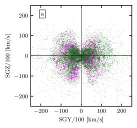
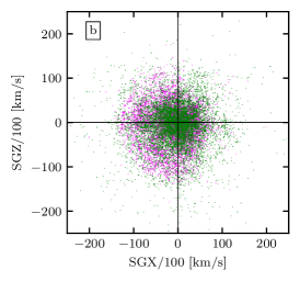
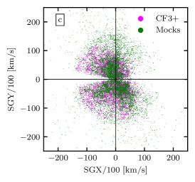
The fidelity of the mock to the CF3 catalogue, is shown in Figs. 1 and 2. Fig. 1 shows the three supergalactic projections with the mock data points in green and the CF3 constraints in purple. The Zone of Avoidance (ZOA) and visual distribution of the catalogues are well recovered. Quantitatively this is shown by looking at the distributions of $P({\rm SGB})$, $P({\rm SGL})$ and $P(z)$ themselves shown in Fig. 2a, b, and c, respectively. The distribution of SGB, SGL and $cz$ for the mock galaxies and CF3 constraints, are largely indistinguishable from each other. Fig. 2c shows that within $\sim 20\,h^{-1}\,{\rm Mpc}$, the number of CF3 constraints is much greater than the mock catalogues presented here. This is because of there are too many CF3 constraints in this region, with respect to the resolution of our simulation.

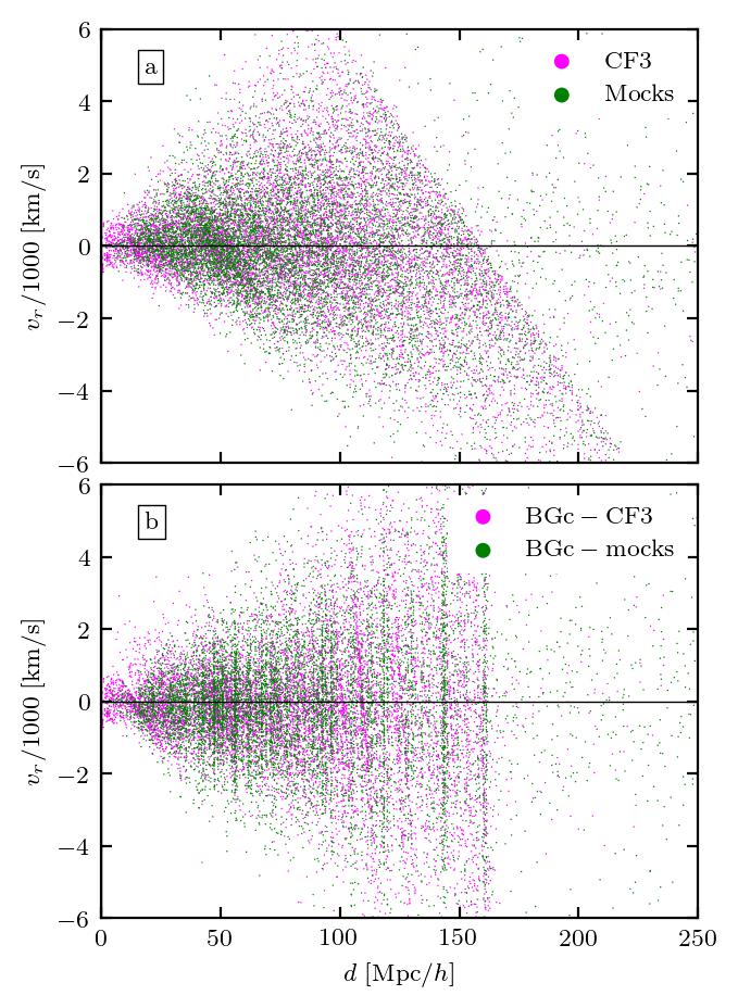
In principle the original unperturbed $d$, $d_{L}$, $\bar{z}$ and $v_{r}$ for each halo that in the mock can be “forgotten” and new values can be computed using the values of $z$ and $\mu$ that include the observational errors. These new values should exhibit similar biases to the observational data by construction. This is seen in Fig. 3, where the radial velocity as a function of distance is plotted. The diagonal cut in this plot is indicative of the log normal bias dicussed in Section 2.2. At a given distance there is an unequal number of galaxies moving towards and away from the observer, making it appear that the universe is contracting in a “breathing mode”. This log normal bias and its correction are presented in Section 2.2.

2.2 The log-normal bias and the Bias Gaussian correction (BGc)

One of the main purposes of constructing such a detailed mock catalogue as described above is to ensure that the log-normal bias is reproduced, thereby allowing us to gauge the ability of the two reconstruction methods to handle this bias. Much hand wringing and literature has been devoted to the handling of biases in peculiar velocity surveys, and we refer the reader to Strauss & Willick (1995) for a comprehensive explanation. Here we briefly explain what the log-normal bias is and how it is handled in the context of the BGc as proposed by Hoffman et al. (2021). We refer the reader to that work for a comprehensive description of the log-normal bias and its correction by the BGc algorithm.

As mentioned, a Gaussian error on the distance modulus transforms into a log-normal error on the luminosity distance (e.g. the inverse of Eq. 3). In other words, if the same galaxy is observed many times, the mean of the different distance measures will not coincide with its actual value. This bias changes the spatial distribution of the galaxies as well as their inferred peculiar velocities. The log-normal bias can be seen in Fig. 3 where the CF3 and mock catalogue peculiar velocity $v_{r}$ is plotted as a function of distance. Beyond around $\sim 70\,h^{-1}\,{\rm Mpc}$, there is no longer symmetry in the distribution of $v_{r}$ about zero: more galaxies have negative $v_{r}$ and the universe naively appears to be collapsing, a so-called “breathing” mode. In theory it can be corrected since the standard $\Lambda$CDM  model makes an explicit prediction that the expected scatter for the radial component of the velocity is roughly $\sigma_{v}\sim 275\,{\rm km/s}$.

The essence of the BGc scheme is to map the log-normal distribution of the inferred distances around their respective redshift distances into a normal distribution around the median of the log-normal one. The width of that normal distribution is treated as a free parameter set to be $\sim 2\,h^{-1}\,{\rm Mpc}$, in agreement with the $\Lambda$CDM  prediction that the intrinsic scatter of the radial velocities is $\sigma_{v}\sim 275\,{\rm km/s}$. The same procedure is applied to the observed radial velocities, retaining the median of the distribution of the radial velocities of data points in a given redshift bin. Yet for the velocities, unlike the inferred distances, the variance of the distribution is preserved as well. Namely the log-normal distribution of the observed distances is mapped to a Gaussian distribution, while preserving the median of the log-normal distribution. It is the invariance of the median under the normal - log-normal transformation which constitutes the backbone of the BGc scheme. After the application of the BGc scheme to the data, the breathing mode dissapears and the radial peculiar velocities scatter normally about 0 as can be seen in Fig. 3, bottom panel.

Figure 5: Scatter plots of the residual of the BGc/WF (panel a), of the Hamlet  (panel b) and of the WX/WF (panel c) reconstructed $v_{r}$s evaluated at the data points. The residual of the BGc/WF from the Hamlet  reconstructed $v_{r}$s at the data points is shown as well (panel d).

2.3 Wiener Filter and Constrained Realizations (WF/CRs)

The WF/CR method is a tried and tested algorithm for reconstructing the large scale density distribution of the universe, based on a limited number of peculiar velocity measurements. We refer the reader to the voluminous literature (Hoffman & Ribak, 1992; Zaroubi et al., 1995, 1999) reviewing just the essentials here.

The WF is a Bayesian estimator of the underlying velocity field (and associated over-density) given a set of observed radial velocities and a given assumed prior model of the distribution of the peculiar velocities. In cosmological applications of the WF the $\Lambda$CDM  concordance cosmological model is taken to be the prior model. Accordingly: (a) the WF provides the most probable continuous density and 3D velocity fields given a finite number of observed “noisy” radial velocities and the assumed $\Lambda$CDM  model; (b) the CRs sample the constrained residual around the WF field; and (c) the WF and CRs act so as to interpolate between data points and then extrapolate beyond it.

The WF/CRs methodology recovers the linear density and 3D velocity fields. In this context, the over-density field and the 3D velocity are linked through the linearized coupled continuity and Poisson equations

$$\delta=-\bm{\nabla}\cdot\bm{v}/H_{0}f(\Omega_{m}),$$ (5)

where $f(\Omega_{m})$ is the linear growth factor. At large scales, or at early cosmological times, the linear over-density is a good approximation for the fractional over-density, $\delta=\rho/\bar{\rho}-1$, where $\rho$ is the density and $\bar{\rho}$ is the cosmological mean. Unless stated otherwise, all the terms density and velocity refer to the linear density and velocity fields density. However, linear theory is clearly violated on small scales. Additionally, the density field is more susceptible to non-linear dynamics than the velocity field. The linear WF/CRs constitute a reasonable estimate of the actual velocity field down to the scale of roughly $5-10\,h^{-1}\,{\rm Mpc}$ (Zaroubi et al., 1999).

The WF estimator is the outcome of the “tug-of-war” between the data and the assumed prior, $\Lambda$CDM  in the present case. Where the data is has small errors, the estimated WF field is “close” to the input data point. Otherwise, where the data is weak the WF solution is dominated by the prior model, namely the solution tends to the mean density and null velocity fields. Consequently the constrained variance, i.e variance spanned by the CRs, is small in the good data regime and converges towards the cosmic variance as the data deteriorates.

2.4 Wiener Filter reconstruction from Exact data (Ex/WF)

As there exist no possibility to homogenize the sampling (namely the Zone of Avoidance will always inhibit full sky coverage), the only source of uncertainty that could, one day, be mitigated, is the observational uncertainty in the distance measurement. In order to test the methods’ inherent ability to reconstruct the underlying fields, an additional “method” is compared: the exact WF (hereafter labeled Ex/WF). This is the WF applied to a mock where the error on each data point has been artificially set to zero (and thus no BGc scheme is applied). This serves the purpose of testing the WF in the case where the only source of uncertainty is the sampling. In other words in Section 3, the reconstruction based on the BGc/WF, the Ex/WF and the Hamlet  method are presented.

2.5 Hamlet 

The second approach examined here utilizes a Hamiltonian Monte Carlo sampling of the posterior PDF via the HAmiltonian Monte carlo reconstruction of the Local EnvironmenT (Hamlet ​​) code, which is described in full in Valade et al. (2022).

Unlike the WF/CRs formalism, the Hamlet  algorithm treats the real distances of the data as unknown dynamical variables that need to be estimated, much in the same way as the density and velocity field. It is Bayesian in nature because an ab initio PDF of the variables that are to be estimated can be specified.

A Monte-Carlo technique is used to sample the various posterior PDFs that are under consideration: the cosmic density field, the velocity field and as the distances of the constraining data. The technical challenges of the Monte Carlo approach is twofold. First the (assumed) prior and posterior PDFs of the density and velocity field need to be extended to also include the distribution of distances. Then an efficient sampling of the posterior PDF needs to be devised. Given the extremely high dimensionality of the problem, the Hamiltonian Monte Carlo algorithm is the tool of choice to perform that sampling, outperforming Metropolis Sampling or Gibbs Sampling algorithms by many orders of magnitude (Valade et al., 2022).

Beyond its inhomogeneous distribution (e.g. the ZOA) the CF3+ catalogue has a fairly sharp cut off at around a redshift distance of $150\,h^{-1}\,{\rm Mpc}$ (see Fig. 2c). In practice this defines and limits the extent within which the Hamlet  reconstruction method is valid. Hinton et al. (2017) investigated the problem that occurs when sampling from a distribution that has an abrupt cut off. They show that the reconstructed fields (and inferred variables) close to the cut off will be biased, effectively nullifying the applicability of the reconstruction beyond a small amount closer than the cut off (say $\sim 90\%$). It is therefore expected that any reconstruction based on these data will not be valid beyond around $150\,h^{-1}\,{\rm Mpc}$.

3 Results

Figure 6: A comparison of the of the BGc/WF (left column), Ex/WF (central column) and the Hamlet  (right column) reconstructed over-density fields with the target simulation. For consistency, the over-density plotted for the target field is the linear over-density i.e. the divergence of the velocity field. The middle panels present the reconstructed $\delta$ and the bottom ones show the constrained variance normalized by the cosmic variance, $\Sigma_{\delta}/\sigma_{\delta}$. All plots refer to the $SGZ=0$ plane of the target simulation and all fields are Gaussian smoothed with a $5\,h^{-1}\,{\rm Mpc}$ kernel.

Figure 7: Density scatter plots of $\delta$ reconstructed versus $\delta$ target. Rows from bottom to top: Hamlet , Ex/WF BGc/WF. Columns from left to right: within spheres of $40$, $80$, $120$, $160\,h^{-1}\,{\rm Mpc}$. The red line represents the best fitted line whose line equation is $y=ax+b$. The parameters of the line and the Pearson correlation coefficient are given in the legend. The black line $y=x$ is shown for reference.

Figure 8: Statistics per shell of distance. Absolute value of the coefficient of correlation for $\delta$ between the different reconstructions and the target field. The error envelope represents the $2\sigma$ variation of the ensemble of realizations.

The results are presented in three sub-sections where we (a) compare how the predicted constraints themselves differ from their real values (Section 3.1); (b) examine the accuracy of the reconstruction of the cosmic fields (Section 3.2); and (c) compare the reconstructed monopole and dipole (i.e. bulk flow) multipoles with their target counterparts (Section 3.3).

3.1 Reconstructed data

After applying the BGc/WF and Hamlet  methods to the mock catalogues (as well as the WF to the exact, no error mocks), the first things to check is how well the distributions of radial peculiar velocities, distances and redshifts of the data points, match their target values. This is shown in Fig. 4a,b and c, respectively, where the target curve represents the true distributions of the mock catalogue; namely, the closer the BGc/WF or the Hamlet  curve is to the target, the more accurate the reconstructions. The values of the reconstructed $v_{r}$’s of the mock data points are obtained by interpolation over the grid points. The distances are obtained differently for the different methods. The Ex/WF’s distances are the true distances, thus they are identical to the target. For the BGc/WF method, the distances are the result of the application of the BGc to the data, before the WF is applied. Finally, for Hamlet , the distance of each constraint is the mean of all the distances sampled over the Monte-Carlo steps.

We remind the reader that the Exact WF (green dashed) represents the limits of the WF method. Fig. 4a shows that the Hamlet  reconstruction method does an exceptional job at recovering the distribution of radial peculiar velocities. Note also that the WF in its purest form too recovers the target distribution. The BGc/WF struggles slightly by narrowing the data’s distribution with a slight over emphasis on smaller values of the peculiar velocity at the expense of the large values. We note, as an aside, that the fact that the target (and hence the reconstructions) are not centered at $v_{r}=0$ is due to the specific nature of the mock observer chosen (i.e. cosmic variance). The BGc/WF suppression of the reconstructed radial velocities of the data points relative to the target is inherent in the WF algorithm, where the estimated signal is the weighted “compromise” between the data and the prior model. Where the data is not very strong the WF estimator is biased towards the null field predicted by the prior.

In Fig. 4b and c the distance and redshift distributions are examined. For both of these quantities the two reconstructions do a remarkably good job at matching the target, rendering their curves practically indistinguishable from the target. Note however that the BGc/WF method tends to “exaggerate” some of the peaks and valleys in the distance distributions (Fig. 4b). All models reliably follow the input’s form. In the absence of errors, i.e. the Ex/WF case, the reconstructed $v_{r}$’s of the data points should be equal to the input constraints taken from the target simulation (Hoffman & Ribak, 1992).

The slight mismatch between the $v_{r}$ histograms of the Ex/WF and the target seen in Fig. 4 occurs because the Ex/WF histogram is an interpolation over the course grid of the WF.

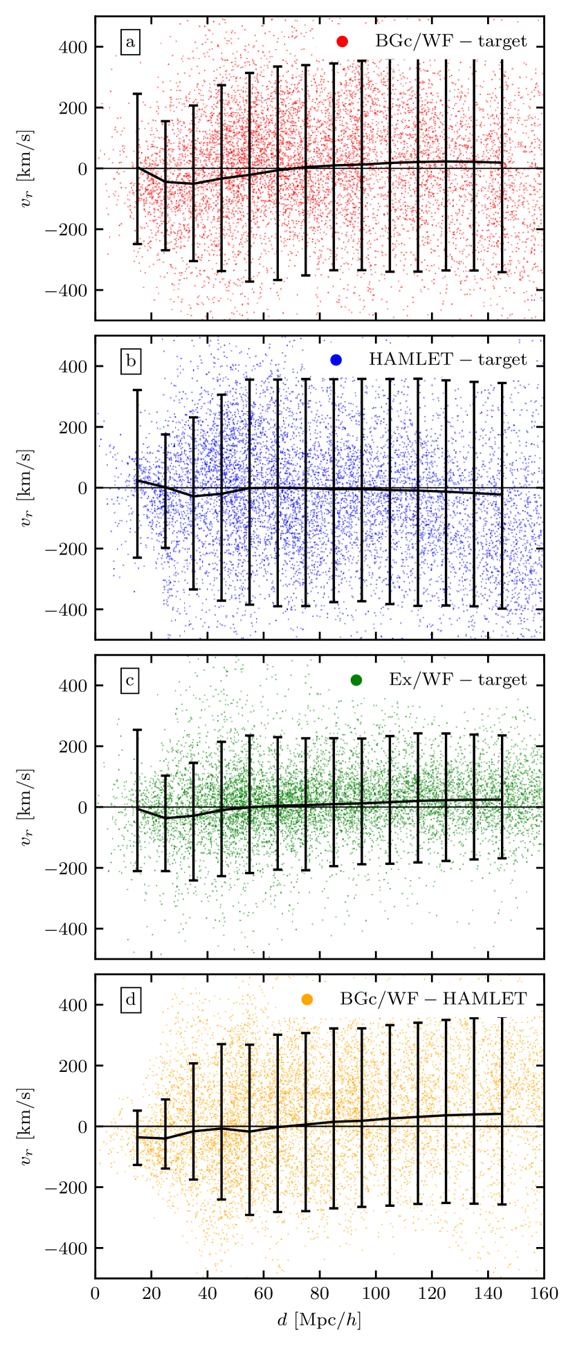
It is important to understand by how much each constraint shifts during the BGc and reconstruction procedures. In Fig. 5 the difference between the reconstructed $v_{r}$ and the input $v_{r}$ is compared on a constraint by constraint basis and as function of distance. From top to bottom this difference is shown for show the BGc/WF, Hamlet and the Ex/WF (respectively Fig. 5a, b and c). The difference between the two main reconstruction methods (BGc/WF and Hamlet ) is shown in the final panel, Fig. 5d. In these plots each constraint is a dot, the mean value of the difference is shown as a black line and the standard deviation of the distribution is designated with error bars. An examination of Fig. 5 reveals that the methods based on the WF tend to underestimate the $v_{r}$ in the inner most distance shells (below $\leq 60\,h^{-1}\,{\rm Mpc}$) while overestimating it in the outer shells. This is sure even for the ideal case of the Ex/WF. The mean of Hamlet  method, however (Fig. 5b) indicates the constraints are not systematically shifted in the region $\sim 40-110\,h^{-1}\,{\rm Mpc}$, but underestimate $v_{r}$ outside this range.

3.2 Reconstructed cosmic fields

In this section the reconstructed density and velocity fields are examined and compared with the target.

Figure 9: Same as Fig. 6 for the radial component of the velocity field.

Figure 10: Same as Fig. 7 for the radial component of the velocity field.

Figure 11: Same as Fig. 8 for the radial component of the velocity field.

Figure 12: The monopole moment (upper panel), the amplitude of the dipole moment (i.e. the bulk velocity; middle panel), and the cosine of the angle of alignment between the reconstructed and target bulk velocities (lower panel) are shown. The profiles present the mean and “$2\sigma$” scatter of the mean profile in spheres of radius $d$. The reconstructions correspond here to the Ex/WF (green dashed line), the BGc/WF (red dotted line) and the Hamlet  (blue dot-dashed line) case. The scatter is the constrained variance of the different reconstruction and the target simulation is presented by the black solid line (middle and upper panels).

3.2.1 Reconstructed density maps

The non-linear density field of the target simulation cannot be directly compared with the reconstructed linear density field. To enable a meaningful comparison we compare the divergence of the velocity field of the two (i.e. Eq. 5), terming both of these $\delta$, out of convenience.

In order to visually inspect the reconstructed density distribution, a $3.9\,h^{-1}\,{\rm Mpc}$ thick slab at the super galactic plane (SGZ=0) is chosen. This is not an arbitrary choice: given that the largest numbers of constraints are expected to lie in or close to SGZ=0, we expect this slab to be the most accurate. The fields are smoothed with a Gaussian kernel of $5\,h^{-1}\,{\rm Mpc}$.

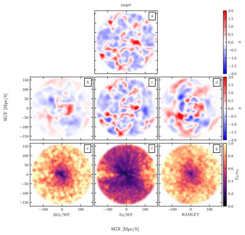
Fig. 6 examines the density distribution in this slab. Fig. 6a is the target density distribution. The column below it (namely the middle column, Fig. 6c, f shows the Ex/WF results, while the left column (Fig. 6b, e) shows the BGc/WF results and the right column (Fig. 6d, g) shows the Hamlet  results. The middle row (panels b, c, d) shows the reconstructed density distribution. Some conclusions may be drawn from a visual examination of Fig. 6b, c, d. The Ex/WF generally recovers the features of the local cosmography at all distances. The reconstruction is not exact; given that there are no “observational” errors here, this implies that the mismatch between the Ex/WF and the target (i.e. between Fig. 6c and Fig. 6a), are entirely due to the finite, inhomogenous and anisotropic sampling. Comparing the BGc/WF (Fig. 6b) with the target indicates a decline of power of the reconstructed density field with the distance from the observer, yet the general structure of the cosmic web of over- and under-dense regions is recovered. The Hamlet reconstructed $\delta$ field does not exhibit the same loss of power as in the BGc/WF case but it suffers from a loss of spatial resolution with distance (Fig. 6d). The more distant structures become more fuzzy and diffuse.

The bottom panels of Fig. 6 present the constrained variance $\Sigma^{2}_{\delta}$ of the three reconstructed $\delta$ fields. It is defined as the local, cell by cell, variance calculated over an ensemble of CRs for the Ex/WF and BGc/WF case and over a set of independent states of the Monte Carlo chain in the Hamlet case. The panels show the square root of constrained variance normalized by the cosmic variance, $\Sigma_{\delta}/\sigma_{\delta}$. The cosmic variance is calculated by calculating the variance over all CIC cells in each reconstructed $\delta$ field. The value of $\Sigma_{\delta}/\sigma_{\delta}$ gauges the constraining power of the constraints and the assumed prior model. When this equals to 0 the region is highly constrained and when it equals unity the reconstructions are as random as cosmic variance. Thus one expects it to be small close to the observer and to approach unity asymptotically with distance.

Fig. 6e, f, g quantifies what is visually apparent from (Fig. 6b, c, d) namely that the inner regions are well constrained but that this fades with increasing distance. The reconstruction methods that include errors (i.e. Fig. 6e,g) are never “perfect”, while the Ex/WF method Fig. 6f, does obtain values of $\Sigma_{\delta}/\sigma_{\delta}$ close to 0. Interestingly, the impact of the ZOA on the reconstruction method is apparent in Fig. 6f. Here it causes a very clear limitation of the expected ability to reconstruct the density field.

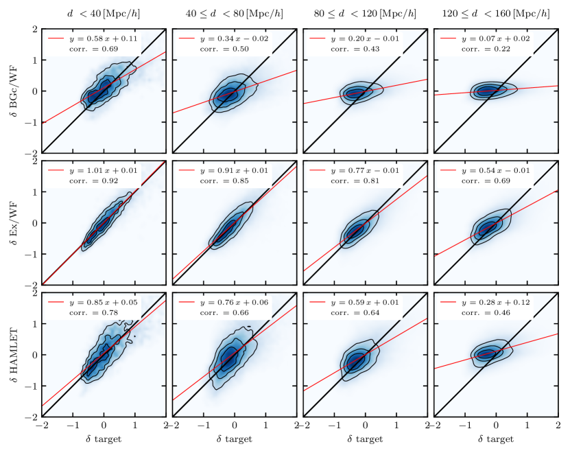
The accuracy of the density field reconstructions - specifically their accuracy as a function of distance - is shown in Fig. 7. These are scatter plots which compare, on a cell by cell basis, the density of the target with the BGc/WF (top row), Ex/WF (middle row) and Hamlet (bottom row). The line, $y=ax+b$, (or $\delta_{\rm method}=a\delta_{\rm target}+b$, to be more precise), which best describes the scatter is shown in red; its slope, $y$ intercept and the Pearson correlation coefficient is given in each sub-panel. In the ideal case where a reconstruction method perfectly matches the target this would simply be a slope of $a=1$ and an offset or bias of $b=0$ line with zero scatter (shown in black), with a Pearson correlation coefficient of unity. The columns in this figure denote different $40\,h^{-1}\,{\rm Mpc}$ thick radial shells under consideration. Note that a slope less than unity indicates that the reconstruction under-estimates the over-dense regions and over estimates the under-dense regions. A slope greater than unity represents the opposite (exaggerates over- and under-dense regions). An offset of $b\neq 0$ means a biased reconstruction.

There are a number of important features of this Fig. 7. First, considering the inner most bin (leftmost column) the Ex/WF reconstruction recovers very well the density of the target. A slope of unity and practically null offset of $b=0.01$ and a correlation coefficient of 0.92 indicates that in general in this region the Ex/WF reconstructions is very well recovered. This implies that the nearby sampling of the CF3 catalog is almost optimal. Obviously, the Hamlet and the BGc/WF methods do worse in recovering the density field. Moving to the outer shells all three density reconstruction systematically degrade with slopes and correlation coefficient decreasing. The slope in all cases is less than unity, indicating that the reconstructions suppress the power of the recovered density field. This diminishing of the power increases with the distance from the observer. The BGc/WF suffers more from the loss of correlation with distance than the Hamlet . Yet, the latter reconstruction is at large distances with $b=0.12$ for the distance range of $120\ \leq\ d\ \leq\ 160\ Mpch$. The BGC/WF behaves, on the other hand, by the “Bayesian book” - where the sampling is very sparse and the errors are much larger than the signal, the unbiased $\Lambda$CDM prior is recovered.

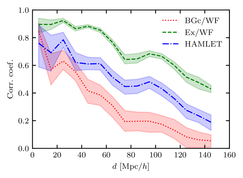
The correlation between the reconstructed mean field and the target is shown as a function of distance in Fig. 8. These are the correlation coefficients from the scatter plots (Fig. 7) plotted as a function of distance in order to gauge the degradation of the reconstruction methods as data becomes more sparse and volumes become large. Note that the binning is different hence the non identical values of the correlation coefficient between the two plots. The solid lines in Fig. 8 represent the mean correlation coefficient between the reconstruction and the target; the error corridor represents the 2$\sigma$ variance about this mean. As expected the Ex/WF is always a superior to the BGc/WF and the Hamlet method. With the exception of the inner most bin, the Hamlet   method achieved higher correlation coefficients than the BGc/WF method. At the edge of the data, no method achieves a correlation coefficient of greater than 0.5.

3.3 Reconstructed radial velocity maps

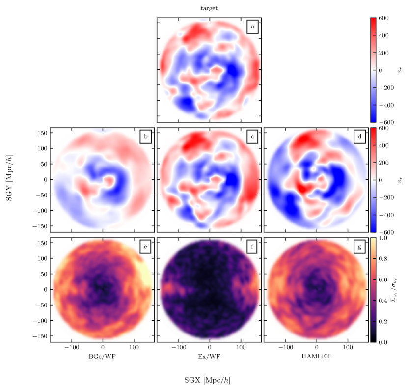
The examination of the radial component of the velocity field follows here that of the density field (§3.2.1). The same $SGZ=0$ and $4\,h^{-1}\,{\rm Mpc}$ thick slab is shown in Fig. 9. Again, the top panel is the target radial peculiar velocity field while the left column shows the BGc/WF reconstruction, the middle column the Ex/WF reconstruction and the right most column, the Hamlet  reconstruction. The fields are smoothed with a Gaussian kernel of $5\,h^{-1}\,{\rm Mpc}$.

The radial velocity field (Fig. 9b, c, d) appears much more accurately reconstructed than the density field. The same outflows and inflows are generally visible and the cosmographic landscape is recognisable in all three cases. Although the reader will note that the accuracy of the velocity reconstruction, like the density field, deteriorates at larger distances. Features are recognisable but distorted and smoothed out.

The constrained and cosmic variances of the radial velocity, $\Sigma_{v_{r}}$ and $\sigma_{v_{r}}$, are calculated much in the same way as in for the density field (§3.2.1). The imprint of the ZOA is clearly seen in the $\Sigma_{v_{r}}/\sigma_{v_{r}}$ map of the Ex/WF map. Yet, in all cases considered here the constrained variance, normalized by the cosmic variance, is much smaller than in the density case. Namely, the velocity field is much more constrained by the CF3 data than the density field. In general the reconstructed Hamlet  velocity field bares a closer resemblance to the target than the BGc/WF reconstruction.

A close inspection of Fig. 9d uncovers one troubling feature. At the edge of the reconstructed volume, at distances close to $150\,h^{-1}\,{\rm Mpc}$ the reconstructed is “bluer” than in the corresponding target and the Ex/WF maps. Namely the Hamlet  reconstructed velocity field has a spurious negative infall. This is a manifestation of the limitation of the method as described by Hinton et al. (2017) in Section 2.5.

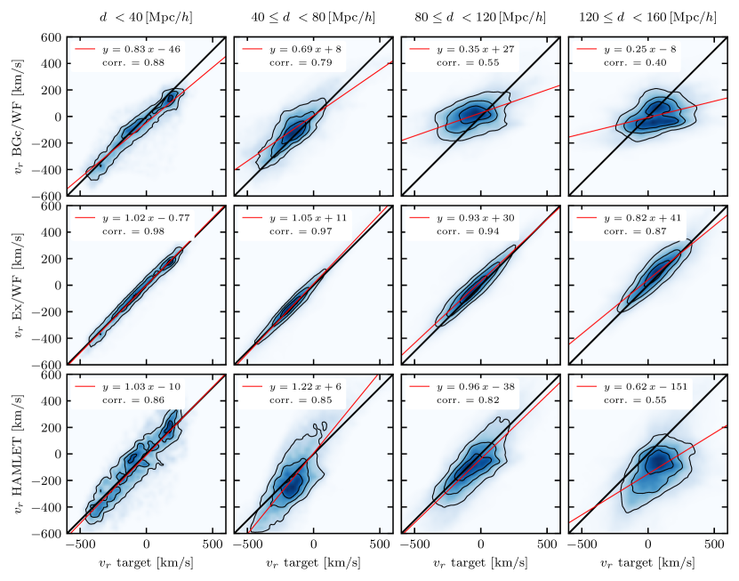
Again, we turn to a scatter plot, on a cell by cell basis to quantify the quality of the reconstruction as a function of distance in Fig. 10, which is structured identically to Fig. 7 - namely radial extent increasing column wise from left to right, while the rows from top to bottom being BGc/WF, Ex/WF and Hamlet . This figure is qualitatively identical to its density field counter part (Fig. 7) in that the same behavioural trends between the different reconstructions methods and as a function of distance exist. The correlation analysis of the Ex/WF and BGc/WF cases behaves much in the same way as for the density field - a degradation of the correlation with distance, a slope ($a$) that is close to unity nearby and diminishes with distance, and essentially with zero offset ($b\sim 0$). Yet, the quality of the reconstruction of the radial velocity is much better than that of the density. The Hamlet  reconstruction shows a somewhat unexpected behaviour. The slope of the best fit line for the distance range of $40\ \leq\ d\ \leq\ 80\ \,h^{-1}\,{\rm Mpc}$ exceeds unity, $a=1.22$, i.e. there is an excess of power compared with the target and the Ex/WF cases. This is unexpected for a Bayesian algorithm. The best linear fit for the range of $120\ \leq\ d\ \leq\ 160\ \,h^{-1}\,{\rm Mpc}$ yields a significant negative offset of $b=-151\,{\rm km/s}$, in agreement with the visual inspection of Fig. 9g.

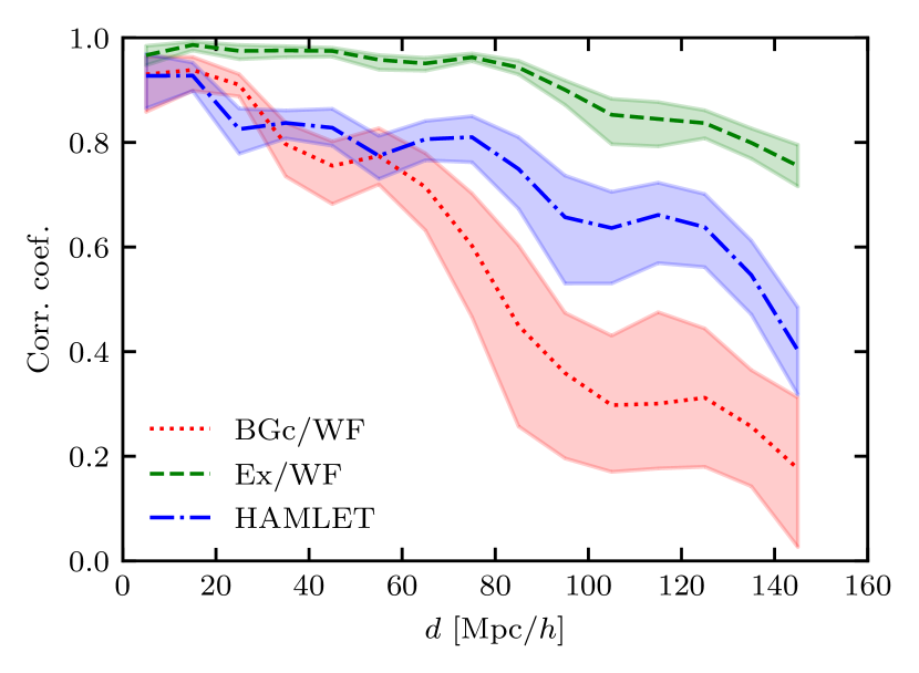
The correlation of the radial component of the velocity field between the reconstructions and the target is shown as a function of distance in Fig. 11. Similar to Fig. 8, these are the correlation coefficients computed from scatter plots (Fig. 10) plotted as a function of distance in order to gauge the degradation of the reconstruction methods as data becomes more sparse and volumes become large. The solid lines in Fig. 11 represent the mean correlation coefficient between the reconstruction and the target; the error corridor represents the 2$\sigma$ variance about this mean. As expected the Ex/WF is always a superior to both the BGc/WF and the Hamlet method. The Ex/WF reconstruction is very well correlated with the target out until $\sim 80\,h^{-1}\,{\rm Mpc}$, beyond which it begins to drop, although it is worth noting that it stays correlated for the full sample. This drop is a manifestation of the sampling and the decreasing number of the data (per volume) at these distances. The Hamlet  and BGc/WF method are roughly equal in the inner regions out to $\sim 70\,h^{-1}\,{\rm Mpc}$, and beyond it the Hamlet  method provides better correlation. At the edge of the data, no method achieves a correlation coefficient of greater than 0.5.

3.4 Multipole moments of the reconstructed velocity field

The first two moments of the velocity field, the monopole and dipole, are examined here. The effect of errors and sampling on the fidelity of these two physical quantities is of particular interest since the monopole and dipole are often used as probes of the scale of homogeneity and can affect probes of the cosmological model in particular.

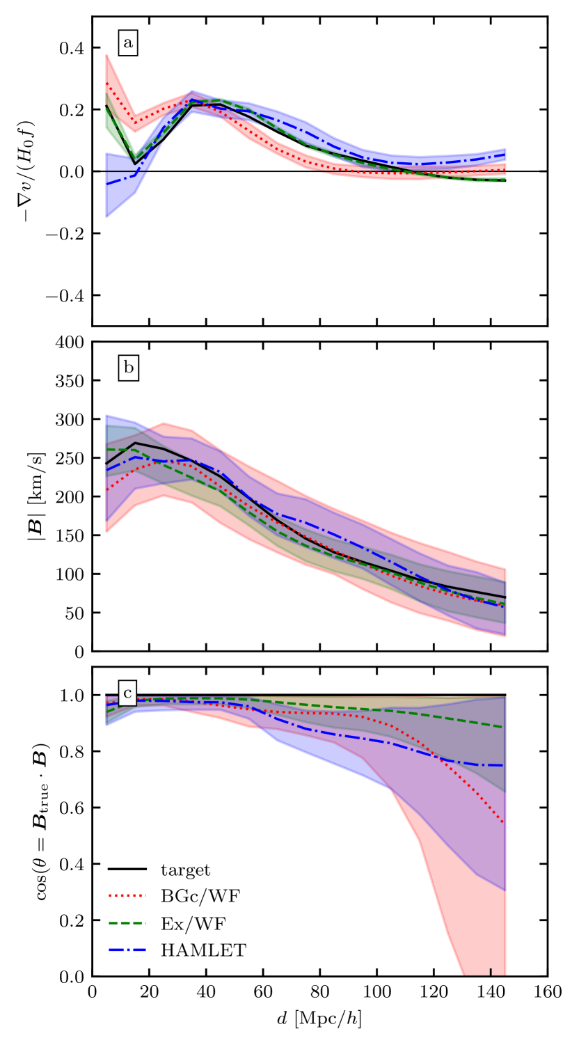
Fig. 12a shows the target and reconstructed velocity monopole as a function of distance. The same colouring and line style convention used in Fig. 8 and Fig. 11 is adopted here too, with the moments of the target simulation plotted in black. Note that the monopole - the mean infall or outflow of matter, is the zeroth order moment of the velocity field. It is the mean of the divergence of the velocity field in spheres of radius $d$ and as such is called the “breathing mode” of the velocity field. In the linear theory of the cosmological gravitational instability the density and velocity fields are related by Eq. 5, hence we opted here to present the monopole term by means of this equations. Thereby, Fig. 12a effectively presents the mean linear density with spheres of radius $d$. The Ex/WF is nearly indistinguishable from the target here: the error corridor (which corresponds to variance across all the constrained realisations) is tiny and the black and green dashed line are practically on top of each other.

The BGc/WF curve overestimates the monopole in the inner parts (within $\sim 50\ \,h^{-1}\,{\rm Mpc}$) while underestimating it outside that range. This increased monopole implies an overestimation of the density in the inner parts of the mock universe, which is confirmed by examining the equation of the best fit line to the scatter plot Fig. 7 (upper row, left column, $d<40\,h^{-1}\,{\rm Mpc}$). The best fit line has has an offset of $b=0.11$, meaning that there is a systematic increase in the estimated densities, consistent with the higher monopole. Both the reconstructions and the target tend to zero infall at these large scales. The Hamlet  method on the other hand behaves inversely to the BGc/WF method, underestimating the target monopole at small scales and over estimating it at large scales. The Hamlet ’s monopole term at the edge of the data reveals an excess of density at $d\sim(120-150)\,h^{-1}\,{\rm Mpc}$, in agreement with Fig. 7 (lower/right panel). Otherwise, the Hamlet  method succeeds in tracking the target monopole over a large range from $\sim 20$ to $\sim 100\,h^{-1}\,{\rm Mpc}$.

Fig. 12b and c shows the second moment of the velocity field, namely the dipole or the bulk flow. Fig. 12b refers to the magnitude of the bulk flow, while Fig. 12c refers to its direction. Accordingly all methods do a fine job of recovering the magnitude of the bulk flow beyond around $\sim 30\,h^{-1}\,{\rm Mpc}$. The Ex/WF has, predictably, a smaller error corridor than the other two methods, which are roughly similar in size. With respect to direction, Fig. 12c shows the dot product between the target bulk flow direction and the reconstructed one (hence in this plot there is no black target line). The bulk flow directions for the Hamlet  and BGc/WF method are aligned to within $\sim 15$ deg of the target out to a distance of $\sim 50\,h^{-1}\,{\rm Mpc}$, while the Ex/WF is well aligned to greater distances. Note that however, even the Ex/WF curve begins to deviate significantly at the reconstructed edge. This indicates that even in the best case scenario of zero errors, sampling at these great distances is a limiting factor in terms of recovering the direction of the cosmic dipole. Note that the accuracy recovered here is also restricted in its ability to recover the underlying dipole direction by the limited depth of the survey (Nusser et al., 2014). The problem is exacerbated when examining the BGc/WF and Hamlet  curves at large distances. Fig. 12 indicates that although the monopole and dipole are well recovered across a large range, the direction of the reconstructed dipole begins to deteriorate when the sampling drops.

4 Summary

The reconstruction of the large scale density and velocity fields from Cosmicflows-like databases of galaxy distances, and hence peculiar radial velocities, is challenging. The data is sparse, extremely noisy with Noise/Signal ratio larger than a few for the majority of the data, non-uniformly and anisotropically distributed. Furthermore the data suffers from the log-normal bias, which leads to a non-linear bias in the estimated distances and velocities.

A number of independent methods have been developed to reconstruct the local LSS and to produce constrained initial conditions for cosmological simulations designed to reproduce our local patch of the Universe (i.e Sorce et al., 2015). What is generally missing from the literature in this field is an understanding of the accuracy of these methods. Often the reconstructions are applied directly to observational data and only very limited conclusions can be drawn on the viability of a cosmography. The present paper compares the BGc/WF (Hoffman et al., 2021) and the Hamlet  algorithms (Valade et al., 2022) by testing them against a carefully crafted mock of an observational catalogue (an improved CF3-like survey) drawn from one the MultiDark cosmological simulations.

The quality of the reconstruction is gauged by studying the residual between the reconstructed and target density and velocity fields. The residual is mostly analyzed by quadratic measures and as such it is characterized by the mean and variance of the distribution. An optimal reconstruction should make the mean of the residual to be as close as possible to the null field and aim at minimizing its variance. A related measure is the linear correlation analysis which yields the best “line”, $y=ax+b$, that fits the linear dependence of reconstructed field on the target one, and the Pearson correlation coefficient. The values of the offset, $b$, for the case of the linear over-density and for the radial velocity are consistent with zero fro the BGc/WF, in agreement with the theoretical expectations. The distant data points are extremely noisy and very sparsely distributed, hence the WF reconstruction is dominated by the $\Lambda$CDM  prior model. The Hamlet ’s significant offset is however inconsistent with the prior model.

We define here three different regions: the nearby ($d\lesssim 40\,h^{-1}\,{\rm Mpc}$), the intermediate (($40\lesssim d\lesssim 120\,h^{-1}\,{\rm Mpc}$) and the distant one ($d\gtrsim 120\,h^{-1}\,{\rm Mpc}$). Based on the above criteria we conclude that nearby the BGc/WF and the Hamlet  methods are doing roughly equally well. The methods diverge at large distance - with the Hamlet  outperforming the BGc/WF with a tighter correlation and smaller variance but underperforming in terms of the bias. This is most noticeable for distant region (the right columns of Fig. 7 and Fig. 8).

The three panels of Fig. 12 deserve a special attention here. The upper panel shows the radial profile of the monopole moment. The four profiles shown there - target, Ex/WF, BGc/WF and Hamlet  - are all constructed under the assumption of $\Lambda$CDM  value of $H_{0}=67.7\,{\rm km/s/Mpc}$. Yet, the negative offset of the monopole moment at the edge of the data implies that the local value of $H_{0}$ is somewhat smaller than its global value. A phenomenon expected for any finite volume realization in the $\Lambda$CDM  cosmology (see Hoffman et al. (2021) for a quantitative assessment). A proper adjustment of the local value of $H_{0}$ would bring the target and Ex/WF profiles to converge to zero at the edge of the data, together with the BGc/WF asymptotic value. This would leave the Hamlet  positive offset standing out with a systematic bias. The amplitude of the dipole moment, namely the bulk velocity, is recovered equally well by the three reconstruction and is in very good agreement with the target. The bottom panel shows the cosine of the angle between the reconstructed and the target bulk velocities. The BGc/WF behaves as expected - the mean misalignment is consistent with the full alignment to within one $\sigma$ of the constrained variance. This is not the case with the Hamlet  reconstruction, where the misalignment is more than $2\sigma$ away from the expected alignment.

Our overall assessment of the Hamlet  and the BGc/WF reconstructions is that the former outperforms the latter one in terms of reduced scatter and tighter correlation between the reconstructed and the target density and velocity fields. Yet, the Hamlet  suffers from biases in the reconstructed LSS at the distant regime - ones that do not appear in the BGc/WF reconstruction. It follows that the Hamlet  should be the method of choice for the reconstruction of the LSS and the study of the cosmography of our local patch of the Universe. The BGc/WF reconstruction is the preferred tool for performing quantitative analysis and parameters estimation and possibly also for setting initial conditions for constrained cosmological simulations. One last comment is due here. The WF/CRs is a very well tested approach that is based on a solid theoretical foundations (Hoffman & Ribak, 1992; Zaroubi et al., 1995, 1999). As such it provides an attractive framework for performing Bayesian reconstruction of the nearby LSS. Yet, any bias in the observational data and in particular the log-normal one needs to be addressed and apply outside that framework in some ad-hoc and approximate way. The HMC methodology, and in particular its Hamlet  implementation, still suffer from some teething problems that need to be overcome. The ability of the MCMC methodology in general and the HMC in particular to address the issue of reconstruction of the LSS, the handling of observational biases and the estimation of cosmological parameters within one computational self-consistent framework makes Hamlet  a very attractive tool in the CLUES’ toolbox. The incredible improvement in the computational efficiency of the Hamlet  compared with previous implementation of MCMC algorithms makes it even more promising for future implementations within the CLUES project.

Data availability

The data underlying this article will be shared on reasonable request to the corresponding author.

References

- Ade et al. (2016) Ade P. A. R., et al., 2016, Astronomy & Astrophysics, 594, A13
- Bertschinger & Dekel (1989) Bertschinger E., Dekel A., 1989, ApJ, 336, L5
- Boruah et al. (2021a) Boruah S. S., Lavaux G., Hudson M. J., 2021a, arXiv e-prints, p. arXiv:2111.15535
- Boruah et al. (2021b) Boruah S. S., Hudson M. J., Lavaux G., 2021b, MNRAS, 507, 2697
- Carrick et al. (2015) Carrick J., Turnbull S. J., Lavaux G., Hudson M. J., 2015, MNRAS, 450, 317
- Davis & Scrimgeour (2014) Davis T. M., Scrimgeour M. I., 2014, Monthly Notices of the Royal Astronomical Society, 442, 1117
- Davis et al. (1985) Davis M., Efstathiou G., Frenk C. S., White S. D. M., 1985, The Astrophysical Journal, 292, 371
- Dupuy et al. (2019) Dupuy A., Courtois H. M., Kubik B., 2019, MNRAS, 486, 440
- Feldman et al. (2010) Feldman H. A., Watkins R., Hudson M. J., 2010, MNRAS, 407, 2328
- Ganon & Hoffman (1993) Ganon G., Hoffman Y., 1993, ApJ, 415, L5
- Graziani et al. (2019) Graziani R., Courtois H. M., Lavaux G., Hoffman Y., Tully R. B., Copin Y., Pomarède D., 2019, Monthly Notices of the Royal Astronomical Society, 488, 5438
- Hinton et al. (2017) Hinton S. R., Kim A., Davis T. M., 2017, arXiv e-prints, p. arXiv:1706.03856
- Hoffman & Ribak (1992) Hoffman Y., Ribak E., 1992, The Astrophysical Journal, 384, 448
- Hoffman et al. (2016) Hoffman Y., Nusser A., Courtois H. M., Tully R. B., 2016, MNRAS, 461, 4176
- Hoffman et al. (2018) Hoffman Y., et al., 2018, Nature Astronomy, 2, 680
- Hoffman et al. (2021) Hoffman Y., Nusser A., Valade A., Libeskind N. I., Tully R. B., 2021, MNRAS, 505, 3380
- Jaffe & Kaiser (1995) Jaffe A. H., Kaiser N., 1995, ApJ, 455, 26
- Kaiser (1987) Kaiser N., 1987, MNRAS, 227, 1
- Lavaux (2016) Lavaux G., 2016, Monthly Notices of the Royal Astronomical Society, 457, 172
- Libeskind et al. (2020) Libeskind N. I., et al., 2020, Monthly Notices of the Royal Astronomical Society, 498, 2968
- Lilow & Nusser (2021) Lilow R., Nusser A., 2021, MNRAS, 507, 1557
- Nusser & Davis (2011) Nusser A., Davis M., 2011, ApJ, 736, 93
- Nusser et al. (2014) Nusser A., Davis M., Branchini E., 2014, ApJ, 788, 157
- Pike & Hudson (2005) Pike R. W., Hudson M. J., 2005, ApJ, 635, 11
- Prideaux-Ghee et al. (2022) Prideaux-Ghee J., Leclercq F., Lavaux G., Heavens A., Jasche J., 2022, arXiv e-prints, p. arXiv:2204.00023
- Qin et al. (2019) Qin F., Howlett C., Staveley-Smith L., Hong T., 2019, MNRAS, 482, 1920
- Riebe et al. (2013) Riebe K., et al., 2013, Astronomische Nachrichten, 334, 691
- Sawala et al. (2021) Sawala T., Jenkins A., McAlpine S., Jasche J., Lavaux G., Johansson P. H., Frenk C. S., 2021, MNRAS, 501, 4759
- Sorce et al. (2015) Sorce J. G., et al., 2015, Monthly Notices of the Royal Astronomical Society, 455, 2078
- Sorce et al. (2016) Sorce J. G., Gottlöber S., Hoffman Y., Yepes G., 2016, MNRAS, 460, 2015
- Strauss & Willick (1995) Strauss M. A., Willick J. A., 1995, Phys. Rep., 261, 271
- Tully et al. (2014) Tully R. B., Courtois H., Hoffman Y., Pomarède D., 2014, Nature, 513, 71
- Tully et al. (2016) Tully R. B., Courtois H. M., Sorce J. G., 2016, The Astronomical Journal, 152, 50
- Tully et al. (2019) Tully R. B., Pomarède D., Graziani R., Courtois H. M., Hoffman Y., Shaya E. J., 2019, The Astrophysical Journal, 880, 24
- Valade et al. (2022) Valade A., Hoffman Y., Libeskind N. I., Graziani R., 2022, MNRAS, 513, 5148
- Yepes et al. (2009) Yepes G., Martínez-Vaquero L. A., Gottlöber S., Hoffman Y., 2009, in Balazs C., Wang F., eds, American Institute of Physics Conference Series Vol. 1178, 5th International Workshop on the Dark Side of the Universe. pp 64–75, doi:10.1063/1.3264558
- Zaroubi et al. (1995) Zaroubi S., Hoffman Y., Fisher K. B., Lahav O., 1995, The Astrophysical Journal, 449, 446
- Zaroubi et al. (1999) Zaroubi S., Hoffman Y., Dekel A., 1999, ApJ, 520, 413