On the response of the Einstein Telescope
to Doppler anisotropies

Abstract

We study the response function of the Einstein Telescope to kinematic Doppler anisotropies, which represent one of the guaranteed properties of the stochastic gravitational wave background. If the frequency dependence of the stochastic background changes slope within the detector frequency band, the Doppler anisotropic contribution to the signal can not be factorized in a part depending on frequency, and a part depending on direction. For the first time, we study the detector response function to Doppler anisotropies without making any factorizable Ansatz. Moreover, we do not assume that kinematic effects are small, and we derive general formulas valid for any relative velocity among frames. We apply our findings to three well-motivated examples of background profiles: power-law, broken power-law, and models with a resonance motivated by primordial black hole scenarios. We derive the signal-to-noise ratio associated with an optimal estimator for the detection of non-factorizable kinematic anisotropies, and we study it for representative examples.

1 Introduction

Once a stochastic gravitational wave background (SGWB) will be detected – see [1] for current prospects – the next goal for GW science will be to characterize its anisotropies. As for the cosmic microwave background (CMB), the anisotropies of the SGWB promise to provide information on the origin and evolution of the GW signal. SGWB anisotropies can be produced by the mechanisms that source the SGWB [2, 3, 4, 5, 6, 7, 8, 9, 10, 11, 12, 13, 14], or by propagation effects through a perturbed universe [15, 16, 17, 18, 19, 20, 21, 22]. Alternatively, they can have a kinematical origin, being induced by the detector motion with velocity $\vec{v}$ with respect to the rest frame of the SGWB. In this work we focus on this last kind of SGWB anisotropies, which have been recently theoretically investigated in [23, 24, 25] (see also [26, 27] for applications and further developments).

The fact that Doppler anisotropies can be relevant for observations of stochastic backgrounds is made manifest by the CMB kinematic dipole, whose amplitude is around two orders of magnitude larger than that of CMB intrinsic anisotropies [28, 29, 30, 31]. For the case of SGWB, in absence of detection, we do not yet know how sizeable SGWB Doppler anisotropies can be. The velocity $\vec{v}$ among the SGWB and our frames could be large: think for example of a SGWB produced in the early universe, during a phase transition within a cosmic fluid in relativistic coherent motion (see e.g. [32, 33] for general reviews on SGWB sources).

At the moment, given our ignorance on possible sources of SGWB, it is then wise to keep non-committal on the relative speed $\vec{v}$, and on the SGWB intrinsic properties. In order to forecast prospects of detection of Doppler anisotropies, the first step is to investigate the response of GW experiments to their possible features. Previous articles studied in detail the response of GW detectors to anisotropies, starting with [34, 35, 36, 37, 38, 39, 40, 41, 42, 43, 44] (see [45] for a general review). Usually, one assumes a factorizable Ansatz for the quantities describing the anisotropic signal. The signal should be described in terms of a contribution depending on GW frequency, times a contribution depending on GW direction only. However, in general, such an Ansatz is not suitable for describing Doppler anisotropies. In fact, building on [24], we show explicitly that if the SGWB slope changes within the detector frequency band – a very common possibility both for astrophysical and cosmological sources (see e.g. [46] in the context of LISA) – the aforementioned factorizable Ansatz is violated.

In this work we outline a method for studying the general case, making use of special simplifying conditions (first pointed out in [47]) for characterizing the study of SGWB with the Einstein Telescope [48, 49]: we apply it to the case of kinematic anisotropies. Our method does not implement any factorizable Ansatz, nor makes the hypothesis that the speed $\vec{v}$ among frames is small. We are able to express the detector response function to an anisotropic signal in terms of combinations of detector properties (the arm directions) contracted with the velocity vector $\vec{v}$: see sections 2 and 3. In particular, we find that the Einstein Telescope response depends in a non-linear (but computable) way on $\vec{v}$ as well as on the frequency dependence of the SGWB profile. As a byproduct, our findings indicate that SGWB Doppler anisotropies can provide us with independent measurements of key features of the SGWB.

We proceed in section 4 investigating the ET response function to three explicit examples of SGWB with well motivated frequency profiles: power law, broken power law (see e.g. [50] for a survey), and models with a resonance, motivated by second-order SGWB induced by the formation of primordial black holes (see e.g. [51, 52, 53, 54]). In section 5 we determine an optimal estimator for detecting Doppler anisotropies, exploiting the characteristic daily modulation of kinematic anisotropies [34]. We obtain the expression for the corresponding optimal signal-to-noise ratio, and we apply our results to representative examples of broken power law SGWB profiles, in order to investigate explicitly how the frequency dependence of the SGWB affects measurements of Doppler effects. Our conclusions in section 6 discuss possible further developments, and are followed by four technical appendixes.

2 Our setup

In order to characterise the interferometer response to Doppler anisotropies, we first present some basic ingredients, and fix the conventions we use for describing the stochastic gravitational wave background (SGWB). We expand the gravitational wave perturbation $h_{ab}(t,\vec{x})$ in Fourier modes as (setting $c=1$)

$$h_{ab}(t,\vec{x})\,=\,\sum_{\lambda}\int_{-\infty}^{+\infty}\,df\,\int d^{2}\hat{n}\,h_{\lambda}(f,\hat{n})\,{\bf e}^{(\lambda)}_{ab}(\hat{n})\,e^{2\pi\,i\,f(t-\hat{n}\cdot\vec{x})}\,,$$ (2.1)

where $\lambda\,=\,(+,\,\times)$ are the polarization indices, $f$ the GW frequency, and $\hat{n}$ a unit vector indicating the GW direction. To ensure that the GW fluctuation is real, we impose $h_{\lambda}(f,\hat{n})\,=\,h^{*}_{\lambda}(-f,\hat{n})$. The polarization tensors satisfy the condition ${\bf e}^{(\lambda)}_{ab}(\hat{n})\,=\,{\bf e}^{(\lambda)\,\,*}_{ab}(-\hat{n})$, and are normalized such that ${\bf e}^{(\lambda)}_{ab}(\hat{n})\,{\bf e}^{(\lambda^{\prime})}_{ab}(\hat{n})\,=\,2\,\delta^{\lambda\lambda^{\prime}}$. The two-point correlator for the Fourier modes $h_{\lambda}(f,\hat{n})$ reads

$$\langle h^{*}_{\lambda}(f,\hat{n})\,h_{\lambda^{\prime}}(f^{\prime},\hat{n}^{\prime})\rangle\,=\,\frac{\delta_{\lambda\lambda^{\prime}}}{2}\,\delta(f-f^{\prime})\,\frac{\delta^{(2)}(\hat{n}-\hat{n}^{\prime})}{4\pi}\,{\cal I}(f)\,{\bf P}(f,\hat{n})\,,$$ (2.2)

with ${\cal I}(f)$ being the GW intensity, an even function of frequency: ${\cal I}(f)\,=\,{\cal I}(|f|)$. The factor ${\bf P}(f,\hat{n})$ accounts for the SGWB anisotropy. Importantly, we do not assume a factorizable Ansatz for ${\bf P}$, and we allow it to be an arbitrary function of $f$ and $\hat{n}$. Our general treatment will suit our analysis of kinematic anisotropies in section 3. Nevertheless, we assume for simplicity that ${\bf P}=1$ if the two-point correlator (2.2) is isotropic, i.e. when the function ${\bf P}$ is independent of the GW direction $\hat{n}$.

The quantity we are interested in is the laser phase difference as measured by a planar ground-based interferometer: in particular, we have in mind the Einstein Telescope (ET) [48]. To characterize this quantity, we follow the discussion of [55] developed for LISA: we adapt it to the case of an anisotropic GW background measured by a ground-based instrument. We consider two arms $AB$ and $AC$ of the interferometer, and indicate with $\Phi_{A_{BC}}$ the phase-difference, as measured at the common vertex $A$. Such a phase-difference can be decomposed into two parts:

$$\Phi_{A_{BC}}(t)\,=\,\Delta\varphi_{A_{BC}}(t)+n_{A_{BC}}(t)\,.$$ (2.3)

In this expression, $\Delta\varphi_{A_{BC}}$ is the GW contribution (if any), and $n_{A_{BC}}$ is the noise. Introducing a standard nomenclature for GW physics (see e.g. [56]), the GW contribution can be expressed as

$$\Delta\varphi_{A_{BC}}(t)\,=\,\sum_{\lambda}\,\int_{-\infty}^{\infty}df\,\int d^{2}\hat{n}\,h_{\lambda}(f,\hat{n})\,e^{2\pi i\,ft}\,F_{A_{BC}}^{(\lambda)}(t,\hat{n})\,,$$ (2.4)

where $F_{A_{BC}}^{(\lambda)}$ is the detector pattern function. We work in a small-frequency limit, suitable for ET [47] for which $2\pi f\,L\ll 1$, with $L$ being the detector arm length. The detector pattern function reads

$$F_{A_{BC}}^{(\lambda)}(\hat{n},t)\,=\,e^{-2\pi\,i\,f\,\hat{n}\cdot\vec{x}_{A}(t)}{\bf e}_{ab}^{(\lambda)}(\hat{n})\,d_{A_{BC}}^{ab}(t)\,,$$ (2.5)

with $d_{A_{BC}}^{ab}$ being the detector tensor,

$$d_{A_{BC}}^{ab}(t)\,=\,\frac{1}{2}\,\left(\ell_{AB}^{a}(t)\ell_{AB}^{b}(t)-\ell_{AC}^{a}(t)\ell_{AC}^{b}(t)\right)\,,$$ (2.6)

and $\ell_{AB}(t)$ indicating the unit vector pointing between $A$ and $B$ vertexes. Notice that the quantity $d_{A_{BC}}^{ab}$ is traceless: $d_{A_{BC}}^{aa}\,=\,0$.

Assuming that noise and GW signals are uncorrelated, the two-point correlation function among phase differences can be expressed as

$$\langle\Phi_{A_{BC}}(t)\Phi_{X_{YZ}}(t^{\prime})\rangle\,=\,\frac{1}{2}\,\int_{-\infty}^{\infty}\,df\,e^{2\pi i\,f(t-t^{\prime})}\,\left[{\cal R}_{A_{BC},X_{YZ}}(f,t,t^{\prime})\,{\cal I}(f)+N_{A_{BC},X_{YZ}}(f)\right]\,.$$ (2.7)

Here $X_{YZ}$ denotes a vertex $X$ between two interferometer arms $XY$ and $XZ$. Those arms can belong to the same instrument as the arms $AB$ and $AC$ (i.e. a single version of the ET interferometer), or instead to a second independent ET-like instrument, as discussed in [47], in order to reduce the correlated noise. Our arguments can in principle apply to both situations. In eq (2.7), ${\cal I}$ is the GW intensity as introduced in eq (2.2), while $N_{A_{BC},X_{YZ}}$ the variance of the noise Fourier transform:

$$\langle\tilde{n}_{A_{BC}}^{*}\,\tilde{n}_{X_{YZ}}\rangle\,=\,\delta(f-f^{\prime})\,\delta^{(2)}(\hat{n}-\hat{n}^{\prime})\,N_{A_{BC},X_{YZ}}\,.$$ (2.8)

The function ${\cal R}_{A_{BC},X_{YZ}}$ in eq (2.7) is the detector response function that we wish to characterize. Collecting the results, such a response function can be expressed as

$${\cal R}_{A_{BC},X_{YZ}}(f,t,t^{\prime}) = \sum_{\lambda}\,\int\frac{d^{2}\hat{n}}{4\pi}\,{\bf P}(f,\hat{n})\,F_{A_{BC}}^{(\lambda)}(\hat{n},t)F_{X_{YZ}}^{(\lambda)}(\hat{n},t^{\prime})$$ (2.9)

$$= {d^{ab}_{A_{BC}}(t)}\,{d^{cd}_{X_{YZ}}(t^{\prime})}\,\Gamma_{abcd}(f)\,,$$

with $d^{ab}$ given in eq (2.6), while

$$\Gamma_{abcd}(f)\,=\,\sum_{\lambda}\,\int\frac{d^{2}\hat{n}}{4\pi}\,e^{-2\pi\,i\,f\,\hat{n}\cdot\Delta\vec{x}}{\bf P}(f,\,\hat{n})\,{\bf e}_{ab}^{(\lambda)}(\hat{n}){\bf e}_{cd}^{(\lambda)}(\hat{n})\,.$$ (2.10)

In eq (2.10), $\Delta\vec{x}$ denotes the spatial difference between the vertexes $A$ and $X$. The response function as defined above depends on the direction-dependent quantity ${\bf P}$ as introduced in (2.2), and controls the anisotropy of the GW correlator. The quantity $\Gamma_{abcd}(f)$ is symmetric under the interchanges $a\leftrightarrow b$, $c\leftrightarrow d$, $ab\leftrightarrow cd$. Moreover, $\Gamma_{aacd}(f)=0$. Eq (2.9) is an extension of well-known formulas (see e.g. [57]) to the case of anisotropic SGWB.

The covariant matrix of phase differences in each vertex can be diagonalized as explained in [47] in the context of the ET interferometer. We refer the reader to this work for details; we do not have anything to add to this topic. After diagonalization, one determines three diagonal channels (called $A$, $E$, $T$), denoted with the letters ${\cal O},{\cal O}^{\prime}$.

We aim at characterizing the response function ${\cal R}_{{\cal O},{\cal O}^{\prime}}(f,t)$ for each diagonal channel: for doing so, we need to analyze the structure of the quantity $\Gamma_{abcd}$ of eq (2.10). For the case of the Einstein Telescope, a major simplification arises, as first found and exploited in [47]. Since the instrument is mostly sensitive to relatively small values of the frequency, $f\sim 7$ Hz, the exponent depending on the vertex distance in eq (2.10) can be neglected. Indeed, we have $|2\pi\,f\,\Delta\vec{x}|\,\simeq\,6\times 10^{-5}\,\left(\frac{f}{\rm Hz}\right)\left(\frac{\Delta x}{\rm km}\right)\,$. This quantity is small (at most of order of percent) for correlations between the arms of a single ET interferometer; or, for correlations between two distinct interferometers located at different places on the Earth surface (but say within continental Europe, see [47]). Under this approximation, in what comes next we are going to determine the structure of the response function of the ET interferometer to Doppler anisotropies of SGWB, with no need to make any factorizable Ansatz for ${\bf P}(f,\hat{n})$, or to assume that kinematic effects are perturbatively small. In fact, we elaborate a method allowing us to compute (2.10), with no need of any expansion in spherical harmonics (which is not too well suited for general scenarios where ${\bf P}(f,\,\hat{n})$ is explicitly frequency-dependent, as ours).

3 ET response function to kinematic anisotropies

Kinematic anisotropies arise from the motion of our GW detector with respect to the rest frame of the SGWB source. These Doppler effects are expected to occur for any background of primordial or astrophysical origin, and can provide the largest anisotropic contribution to a SGWB signal. As a concrete example, for the CMB the amplitude of the kinematic dipole is two orders of magnitude larger than the typical size of intrinsic CMB anisotropies of primordial origin.

For the case of the SGWB, since we are ignorant about its source (if any) and its velocity with respect to us, we prefer to keep non-committal, and derive general formulas which can be applied to generic situations we might encounter. Data, if and when available, will provide information about the relative velocity among frames. We make use of the analytic formulas for kinematic anisotropies recently derived in [24], to obtain results that are valid for any speed of the GW source with respect to us, and for any frequency profile of SGWB signal. (We make the simplifying hypothesis, though, that the GW signal is isotropic in the rest-frame of the SGWB source.)

We indicate with $\Omega_{\rm GW}^{(A)}(f)$ the GW energy density in the rest frame of the SGWB source: as mentioned above, we assume it to be isotropic. The GW energy density becomes anisotropic in a boosted frame $(B)$ moving with velocity $\vec{v}$ wrt $(A)$. In fact, denoting with $\beta\,=\,|\vec{v}|$ (in units with $c=1$) the size of the relative velocity among frames, $\Omega_{\rm GW}^{(B)}$ results [24]

$$\Omega_{\rm GW}^{(B)}(f,\hat{n})\,=\,{\cal D}^{4}\,\Omega_{\rm GW}^{(A)}\left({\cal D}^{-1}\,f\right)\,,$$ (3.1)

with

$${\cal D}\,=\,\frac{\sqrt{1-\beta^{2}}}{1-\beta\,\hat{n}\cdot\hat{v}}\,,$$ (3.2)

and $\hat{n}$ and $\hat{v}$ are the unit vectors along GW direction and the relative velocity of the frame, respectively. Hence, $\Omega_{\rm GW}^{(B)}$ in eq (3.1) is anisotropic, and in general the effects of anisotropy can not be factorized in a part depending on frequency, and another one on direction [24]. Hence the analysis as commonly carried on in previous works should be accommodated to the present situation. Recall that, for the isotropic case, the SGWB energy dependence is related to the GW intensity ${\cal I}(f)$ by

$$\Omega^{\rm isotropic}_{\rm GW}(f)\,=\,\frac{4\pi^{2}\,f^{3}}{3\,H_{0}^{2}}\,{{\cal I}(f)}\,.$$ (3.3)

with $H_{0}$ being the present-day Hubble parameter. Using eq (3.1), we can then conveniently express the GW energy densities in frames $(A)$ and $(B)$ as

$$\Omega_{\rm GW}^{(A)}(f)\,=\,\frac{4\pi^{2}}{3\,H_{0}^{2}}\,f^{3}\,{\cal I}(f)\hskip 17.07182pt;\hskip 17.07182pt\Omega_{\rm GW}^{(B)}(f)\,=\,\frac{4\pi^{2}}{3\,H_{0}^{2}}\,f^{3}\,{\cal I}(f)\,{\bf P}_{\rm kin}(f,\,\hat{n})\,,$$ (3.4)

with (recall the definition (3.2))

$${\bf P}_{\rm kin}(f,\,\hat{n}) = \frac{{\cal D}\,}{{{\cal I}}(f)}\,{{\cal I}}({\cal D}^{-1}\,f)\,.$$ (3.5)

The expression in eq (3.5) demonstrates explicitly that ${\bf P}_{\rm kin}(f,\,\hat{n})$ can not be factorized in a part depending on frequency, times a part depending on direction (unless ${{\cal I}}$ is an exact power law). In fact, if the frequency profile of ${\cal I}$ changes within the detector frequency band, the dependence of (3.5) on ${\cal D}$ (hence on the anisotropy vector $\hat{v}$) changes at the positions where the slope of ${\cal I}$ changes. We will discuss examples of this possibility in the next sections. Notice that if $\beta=0$ (no kinematic anisotropy) then ${\bf P}_{\rm kin}\,=\,1$, as desired.

Fortunately, given the special properties of ET [47] which we discussed at the end of section 2, we can nevertheless derive an exact expression for the ET response function to kinematic anisotropies, with no need of simplifying Ansätze. As we show in the technical appendix A, the interferometer response function (2.9) relative to the $A,E,T$ channels can be expressed as a combination of three terms only, with transparent geometrical meanings:

$${\cal R}_{{\cal O},\,{\cal O}^{\prime}}(f,t,t^{\prime}) = \frac{4}{5}\left[1+\frac{5}{2}c_{1}(f)\right]\,{d^{ab}_{\cal O}(t)\,d_{{\cal O^{\prime}}\,ab}(t^{\prime})}$$ (3.6)

$$+4\,c_{2}(f)\,\left({\hat{v}}_{a}\,{d^{ab}_{{\cal O}}(t)\,d_{{\cal O}^{\prime}\,bc}(t^{\prime})}\,{\hat{v}}^{c}\right)$$

$$+c_{3}(f)\,\left(\hat{v}^{a}\hat{v}^{b}\,d_{ab\,{\cal O}}(t)\right)\,\left(\hat{v}^{c}\hat{v}^{d}\,d_{cd\,{\cal O^{\prime}}}(t^{\prime})\right)\,,$$

with ${\cal O},\,{\cal O}^{\prime}$ denoting the interferometer channels, $d^{ab}$ being the detector tensor (2.6), and $\hat{v}$ the unit velocity vector among the two frames. The quantities introduced in (3.6) read

$$c_{1} = \frac{K_{1}}{8}+\frac{3\,K_{2}}{4}+\frac{K_{3}}{8}\hskip 5.69046pt;\hskip 5.69046ptc_{2}\,=\,\frac{3\,K_{1}}{8}-\frac{3\,K_{2}}{4}-\frac{5\,K_{3}}{8}\hskip 5.69046pt;\hskip 5.69046ptc_{3}\,=\,\frac{3\,K_{1}}{8}-\frac{15\,K_{2}}{4}+\frac{35\,K_{3}}{8}\,,$$

(3.7)

where

$$K_{1} = \int\frac{d^{2}\hat{n}}{4\pi}\left({\bf P}_{\rm kin}-1\right)\hskip 8.5359pt;\hskip 8.5359ptK_{2}=\int\frac{d^{2}\hat{n}}{4\pi}\left({\bf P}_{\rm kin}-1\right)\,(\hat{n}\cdot\hat{v})^{2}\hskip 8.5359pt;\hskip 8.5359ptK_{3}=\int\frac{d^{2}\hat{n}}{4\pi}\left({\bf P}_{\rm kin}-1\right)\,(\hat{n}\cdot\hat{v})^{4}\,.$$

Some comments on the results so far:

• All the effects of kinematic anisotropies in the response function (3.6) are contained in the three terms proportional to the frequency-dependent coefficients $c_{i}(f)$ in eq (3.7). They depend on covariant contractions of the detector tensors $d^{ab}(t)$ with the direction $\hat{v}^{a}$ of the relative frame velocity. Their frequency dependence has important implications when discussing perspectives of detection, as we will discuss in what follows.

• The three independent terms of the response function (3.6) resemble in spirit the effects of the three multipoles $\ell\,=\,(0,\,2,\,4)$ that were found in [47] to contribute to anisotropies detectable by ET. We refrain from elaborating on this analogy in this work, since in our approach we do not implement a multipolar expansion of the anisotropic signal, given that we can not factorize it in frequency times direction. Nevertheless, it would be interesting to understand whether some alternative generalization of the approach of [47] to a non-factorizable Ansatz can lead to results as ours.

• Our method relies on the computation of the three integrals $K_{i}$ in eq (LABEL:def_intK), which can be easily performed by numerical tools, depending on the profile of ${\cal I}(f)$ (recall the definition of ${\bf P}_{\rm kin}$ in eq (3.5)). Notice that they all vanish when $\beta\,=\,0$ (no kinematic effects) or when ${\cal I}(f)$ is a linear function of frequency (see eq (3.5)) . But in general, our formulas are valid for any size of $0\leq\beta<1$, and encompass all kinematic effects with no need of any perturbative expansion in $\beta$.

• The geometrical quantities appearing in the response function (3.6) explicitly depend on time: in particular, the orientation of the detector(s) with respect to the velocity vector $\hat{v}$ experiences daily and annual modulations due to the motion of the Earth. This property will be crucial for determining the optimal estimator sensitive to kinematic anisotropies [34]: see section 5. Interestingly, our general formulas can also describe scenarios where the kinematic parameters $\beta$ and $\hat{v}$ have intrinsic time-dependence (not just due to the Earth motion). It would be interesting in future works to explore whether there can be SGWB sources realizing this possibility.

In the next section 4 we study three well-motivated examples of ${\cal I}(f)$, so as to concretely explore the effects of kinematic anisotropies on the response function of ET.

4 Three examples of SGWB frequency profiles

We apply our methods to three well motivated scenarios for the frequency dependence of ${\cal I}(f)$. We start discussing the case of an exact power-law profile, for which we are able to obtain fully analytic formulas valid for any value of $0\leq\beta<1$. We then continue discussing the cases of single and multiple broken power law, for which the function ${\bf P}_{\rm kin}$ – the quantity controlling the SGWB anisotropy – is not factorizable in parts depending respectively on frequency and direction. In such cases, we compute how anisotropies depend on the frequency profiles of ${\cal I}(f)$, with no restrictions on the size of $\beta$ within the interval $0\leq\beta<1$.

4.1 First example: a power-law SGWB profile

We start by considering a power-law intensity profile in the SGWB rest frame, as described by the Ansatz

$${\cal I}^{PL}(f)\,=\,I_{0}\,\left(\frac{f}{f_{\star}}\right)^{\alpha}\,,$$ (4.1)

where $I_{0}$ is a normalization factor, and $f_{\star}$ is a reference frequency. Relation (4.1) for the intensity implies, through eq (3.3), that $\Omega_{\rm GW}$ scales with frequency as

$$\Omega_{\rm GW}\,\propto\,f^{3+\alpha}\,.$$ (4.2)

The degree of kinematic anisotropy depends on the parameter $\alpha$ in eq (4.1). Making use of eq (3.5), the kinematic anisotropy parameter ${\bf P}_{\rm kin}$ reads

$${\bf P}_{\rm kin}\,=\,\frac{{\cal D}}{{{\cal I}^{PL}}(f)}\,\,{{\cal I}^{PL}}({\cal D}^{-1}\,f)\,=\,{\cal D}^{1-\alpha},$$ (4.3)

confirming that, in this particular case, the dependence on frequency cancels out. The integrals (LABEL:def_intK) can be done analytically, and we can build exact expressions for the quantities $c_{1,\,2,\,3}$ which enter in the response function of eq (3.6), for any values of $\alpha$ and $0\leq\beta\leq 1$. The complete formulas are rather long and we relegate them to Appendix B. In table 1 we present the exact results for the coefficients $c_{i}$ given in eq (3.7) as functions of $\beta$. We make three representative choices of the exponent $\alpha$.

	$\alpha=-3$	$\alpha=3$	$\alpha=5$
$c_{1}$	$-\frac{64\beta^{7}+66\beta^{5}-80\beta^{3}+30\left(\beta^{2}-1\right)^{3}\tanh^{-1}(\beta)+30\beta}{60\beta^{5}\left(\beta^{2}-1\right)}$	$\frac{64}{105}\,\frac{\beta^{2}}{1-\beta^{2}}$	$\frac{8\,\beta^{2}}{315}\,\frac{(81-10\,\beta^{2})}{\left(1-\beta^{2}\right)^{2}}$
$c_{2}$	$\frac{66\beta^{5}-80\beta^{3}+30\left(\beta^{2}-1\right)^{3}\tanh^{-1}(\beta)+30\beta}{12\beta^{5}\left(\beta^{2}-1\right)}$	$-\frac{4}{35}\,\frac{\beta^{2}}{1-\beta^{2}}$	$-\frac{8\,\beta^{2}}{315}\,\frac{(27+4\,\beta^{2})}{\left(1-\beta^{2}\right)^{2}}$
$c_{3}$	$\frac{96\beta^{7}-462\beta^{5}+560\beta^{3}-210\left(\beta^{2}-1\right)^{3}\tanh^{-1}(\beta)-210\beta}{12\beta^{5}\left(\beta^{2}-1\right)}$	$0$	$\frac{8}{315}\,\frac{\beta^{4}}{\left(1-\beta^{2}\right)^{2}}$

Table 1: The $c_{i}$ of eq (3.7) for three choices of exponents in the power-law Ansatz of eq (4.1).

In each case, the absolute value of the size of the anisotropy contributions to the detector response function monotonically increases, as $\beta$ increases towards $\beta\to 1$. The case $\alpha=-3$ corresponds to a scale-invariant GW density parameter, according to eq (4.2).

Notice that, in the small $\beta$ limit, contributions start only at order $\beta^{2}$ (or higher): the ET response is insensitive to linear contributions in $\beta$ to kinematic anisotropies, corresponding to the kinematic dipole. This reflects the fact that ET is insensitive to the dipolar anisotropies [47], at least within the approximation we are interested in.

In this power-law scenario, it is also instructive to investigate how the results vary with the exponent $\alpha$, while having $\beta$ fixed to a representative value. We plot the results in Fig 1, for two choices of the velocity parameter $\beta$, one with $\beta$ large, and one with $\beta$ relatively small. As expected, the amplitude of $c_{i}$ is quite sensitive to the value of $\beta$.

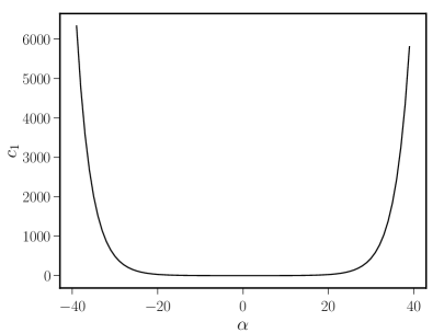
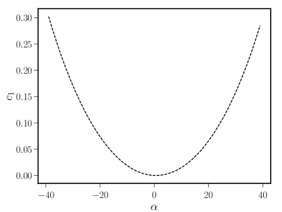
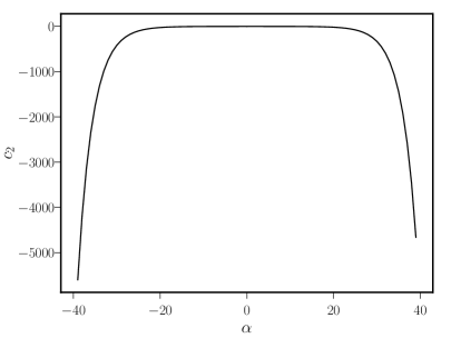
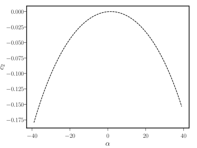
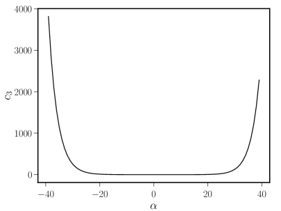
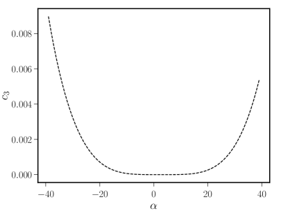
Figure 1: The $c_{i}$ for the power-law Ansatz (4.1). Left plots: We fix $\beta=0.3$ and vary the exponent $\alpha$. Right plots: We fix $\beta=0.04$ and vary the exponent $\alpha$.

The absolute values of the coefficients $c_{i}$ of eq (3.7) increase as the absolute value of $\alpha$ increases. The larger the exponent, the larger the kinematic effects on the anisotropies. For the coefficient $c_{3}$, there is a flat plateau around $\alpha=0$, approximately between $-1\leq\alpha\leq 5$. Such a flat plateau is present for both large and small values of $\beta$. These findings will be useful for interpreting the results of the scenarios we shall discuss next.

4.2 Second example: a broken power-law SGWB profile

We now turn to a broken power-law profile for the GW intensity ${\cal I}(f)$ in the SGWB rest frame. Many examples and realizations of such a profile exist in the literature, see e.g. the survey in [50]. In this case, the role of frequency is important, and kinematic anisotropies can not be factorized as frequency times direction. We consider the following Ansatz for the SGWB intensity as function of frequency [62, 63]:

$${\cal I}^{BPL}(f)\,=\,I_{0}\,\left(\frac{f}{f_{\rm fid}}\right)^{\gamma}\left[1+\left(\frac{f}{f_{\star}}\right)^{\frac{1}{\kappa}}\right]^{-\kappa(\gamma+\delta)}\,.$$ (4.4)

The exponents $\gamma$ and $\delta$ control the growing and decaying parts of the SGWB frequency profiles, respectively. The parameter $\kappa$ controls the smoothness of the transition. The quantity $I_{0}$ is a normalization factor. $f_{\rm fid}$ is a fiducial frequency, and $f_{\star}$ is a parameter controlling the frequency region where the profile changes slope. In Fig 2 we have plotted the SGWB intensity for concrete examples for representative choices of parameters.

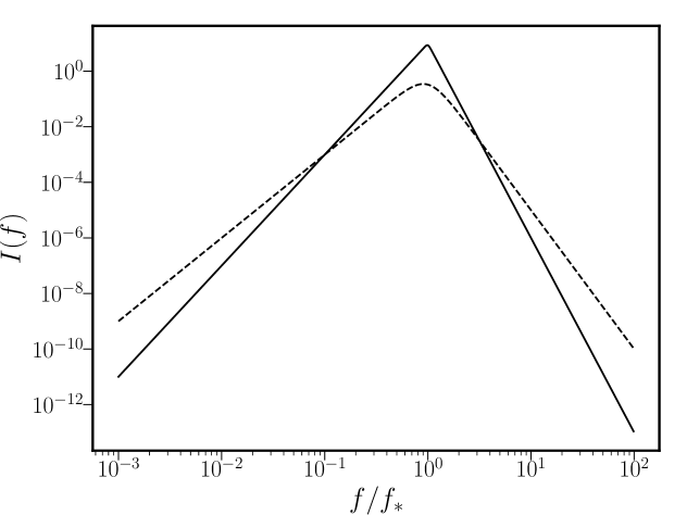
Figure 2: Logarithmic plot of the intensity for a broken power-law profile, eq (4.4). Solid line: $I_{0}=10^{-3}$, $\gamma=4$, $\delta=7$, $\kappa=0.02$, $f_{\rm fid}=f_{\star}/10$. Dashed line: $I_{0}=10^{-3}$, $\gamma=3$, $\delta=5$, $\kappa=0.2$, $f_{\rm fid}=f_{\star}/10$.

For the case of broken power-law, the quantities in eq (LABEL:def_intK) need to be integrated numerically. The coefficients $c_{i}$ in eq (3.6) explicitly depend on frequency. In fact, we expect them to be constant in the frequency ranges corresponding to a constant slope – in the regions of growth and decay of the intensity profile – following the behaviour described in section 4.1. Their non-trivial frequency dependence is amplified as $\beta$ increases. The frequency profiles of the plots in Fig 3 confirm these expectations. Notice that, for the choice of parameters corresponding to the dashed-line plot on the right panel of Fig 2, the size of the quantity $c_{3}$ in Fig 3 is one order of magnitude smaller than $c_{1,2}$. This is due to the fact that the growing and decaying slopes of the corresponding ${\cal I}(f)$ have been chosen to lie in the flat plateau of Fig 1 (right panel). We will reconsider this case in section 5.

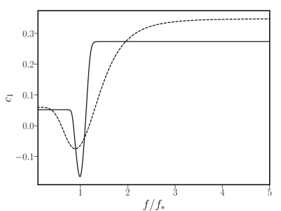
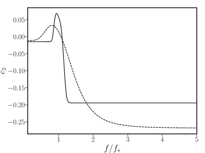
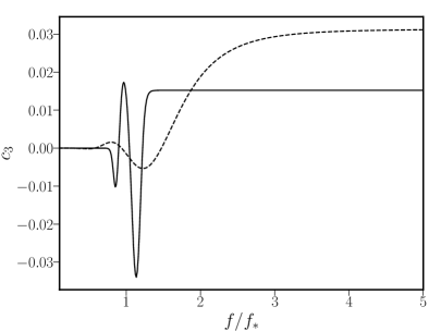
Figure 3: The quantities $c_{i}$ of eq (3.7) for the broken power-law Ansatz (4.4). Solid lines: $\beta=0.2$, and the same parameters as the solid line plot of Fig 2. Dashed lines: $\beta=0.3$, and the same parameters as the dashed line plot of Fig 2.

Furthermore, we also expect that the smaller the parameter $\kappa$ is in our Ansatz (4.4), the sharper the transition among the growing and decaying regions of the intensity profile will be. Therefore, when $\kappa$ is small, the features in the detector response as a function of frequency are further enhanced around $f_{\star}$. Fig 3 confirms these expectations. Notice also that, for sharp transitions, the absolute value of the amplitude of the $c_{i}$ around the transition can be larger than their value in the constant-slope regions (see e.g. fig 3, upper right panel). This indicates that the response function can be sensitive to sudden changes in slope, and kinematic anisotropies can be an indicator of such features.

4.3 Third example: double broken power-law, and resonance

As a last example, we consider a double power-law profile for the SGWB intensity ${\cal I}(f)$. Such a possibility is physically motivated by early-universe scenarios in which a SGWB is induced at second order in perturbations by a scalar power spectrum with a pronounced peak [51, 52, 53, 54]. Such models are frequently investigated in the context of primordial black hole production from inflation – see e.g. [64] for an exhaustive review. Interestingly, if the source scalar peak is sufficiently narrow, the induced SGWB profile has an initial bump, followed by a pronounced, narrow resonance. The details of the bump and of the resonance depend on properties of the source curvature spectrum, as well as on the underlying cosmological expansion. Nevertheless, analytical formulas are available for a number of examples [65, 66, 67]. Effects of Doppler anisotropies in these scenarios have been recently investigated in [24], in the small $\beta$ limit.

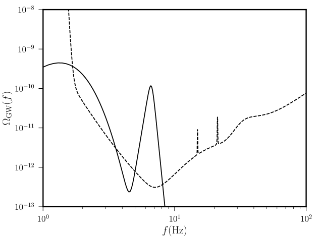
Figure 4: Logarithmic plot of the GW energy density for a double broken power-law profile, eq (4.5) (converted to $\Omega_{\rm GW}$ using eq (3.3)). We have chosen the following values for the parameters: $I_{1}\,=\,9H_{0}^{2}\times 10^{-11}/(8\pi^{2})$, $I_{2}=45H_{0}^{2}\times 10^{-13}/(8\pi^{2})$, $\gamma=4$, $\delta=25$ $\kappa=0.5$, $\gamma_{1}=20$, $\delta_{1}=33$, $\kappa_{1}=0.02$, $f_{1}=1/3$, $f_{\star}=10/3$, $f_{2}=5$, $f_{3}=20/3$ Hz. A mild bump is followed by a pronounced peak. In the dashed line we plot the Einstein Telescope sensitivity curve $\Sigma_{\rm GW}(f)$ to a stochastic background, with one year of data collection. See the discussion around eq (5.15) for explanations.

For simplicity, we model such a scenario in terms of double power-law, essentially duplicating the Ansatz of section 4.2:

$${\cal I}^{DPL}(f)\,=\,I_{1}\,\left(\frac{f}{f_{1}}\right)^{\gamma-3}\left[1+\left(\frac{f}{f_{\star}}\right)^{\frac{1}{\kappa}}\right]^{-\kappa(\gamma+\delta)}+I_{2}\,\left(\frac{f}{f_{\rm 2}}\right)^{\gamma_{1}-3}\left[1+\left(\frac{f}{f_{3}}\right)^{\frac{1}{\kappa_{1}}}\right]^{-\kappa_{1}(\gamma_{1}+\delta_{1})}\,,$$ (4.5)

where $I_{1,2}$ are normalization factors, $f_{1}$, $f_{2}$, $f_{3}$ are fiducial frequencies, and $f_{\star}$ a characteristic frequency around which the first bump occurs. The exponents have the same roles as in the single broken power-law case (see comments after eq (4.4)), controlling the slope of the spectrum. See Fig 4 for a phenomenological profile with the desired features. The position of the resonance has been chosen to lie within the best sensitivity region for the ET-D nominal configuration.

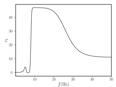
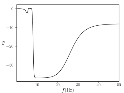
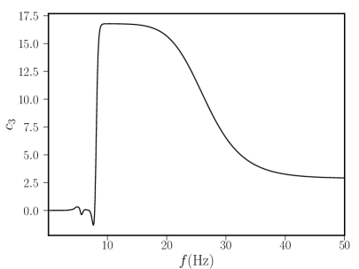
Figure 5: The quantities $c_{i}$ of eq (3.7) for the double broken power-law Ansatz (4.5). We choose $\beta=0.2$, and the remaining parameters are the same as in Fig 4.

With such a rich frequency dependence of the initial spectrum, we can also expect a rich frequency profile of the anisotropy parameters $c_{i}(f)$ of eq (3.6). In proximity of the resonance (the second peak) we expect drastic changes in the amplitude of the $c_{i}$ as a function of frequency, since the slopes of the intensity ${\cal I}(f)$ (or the GW density) reach large values. This expectation is confirmed by our results in Fig 5. In fact, for large slopes, the absolute value of the $c_{i}$ become large (see Fig 1): this property can enhance the prospects of detectability, as we will learn in section 5.3. In comparison, the initial mild bump, at frequencies smaller than the resonance peak, produces small oscillatory effects. Notice that Fig 5 indicates that the absolute values of the $c_{i}$ get larger for an intermediate frequency band, before stabilizing to constant values. The values of the $c_{i}$ are following the slopes of the spectrum as it increases, and then decreases, around the resonance region.

The general formulas we developed in section 3 can also be applied to any further physically motivated Ansätze for ${\cal I}(f)$. In fact, it would be interesting to carry out a more systematic investigation of the ET response function to kinematic anisotropies for a greater variety of frequency profiles. If any of the features associated with the kinematic anisotropy parameters can be detected, they might represent a further indirect probe of the frequency profile of ${\cal I}(f)$, besides direct methods [68]. We plan to investigate these subjects in future works.

5 Detectability and signal-to-noise ratio

In this section we investigate the prospects of detectability of kinematic anisotropies by means of ground-based interferometers, focussing on the Einstein Telescope. Our aim is to determine an optimal estimator for a quantity sensitive to kinematic anisotropies, study the corresponding signal-to-noise ratio, and consider some representative examples of non-monotonic frequency profiles.

We make the hypothesis that noise and GW signal (in the SGWB rest frame) are stationary. But recall that, as we learned in section 3, a feature of the ET response function to kinematic anisotropies is its time-dependence. The orientation of the detector with respect to the velocity vector between the ET and SGWB frames changes with time, following the daily and annual motions of the Earth. Such time-dependence of the signal is precisely the key for determining an optimal estimator sensitive to kinematic anisotropies.

5.1 Disentangling the signal time-dependence

Inspired by the works [34, 47], we start discussing a method to disentangle the daily time-dependence of the signal, and formulate time-independent quantities which are easier to deal with. So far, our results have been presented in a covariant form: see e.g. eq (3.6). To proceed, we choose a convenient reference frame. Let our reference system be anchored to the Earth, with $\hat{z}$ axis along the earth rotation axis. The detector tensors $d^{ab}$ in eq (3.6) are constants, and what varies with time is the velocity vector $\hat{v}$. For any given time $t$, we can split the velocity vector into two parts - one along the $\hat{z}$ axis, and the other perpendicular to it:

$$\hat{v} = \left(\hat{v}\cdot\hat{z}\right)\,\hat{z}+\left[\hat{v}-\left(\hat{v}\cdot\hat{z}\right)\,\hat{z}\right]\,.$$ (5.1)

The vector component parallel to $\hat{z}$, which we dub $\vec{v}_{\parallel}$, does not change with time, being along the Earth rotation axis. The vector component orthogonal to $\hat{z}$, which lies on the plane $(\hat{x},\,\hat{y})$, undergoes a sinusoidal daily modulation with period $T_{e}\,=\,24$ hours. Dubbing $\bar{f}_{e}\,=\,1/T_{e}$ the frequency of the Earth rotation, and indicating with ${\vec{v}}_{\perp}\,\cos{\left(2\pi\,\bar{f}_{e}\,t\right)}$ the time-dependent component of the velocity vector in the plane $(\hat{x},\,\hat{y})$, we can write

$$\hat{v}(t) = {\vec{v}}_{\parallel}+{\vec{v}}_{\perp}\,\cos{\left(2\pi\,\bar{f}_{e}\,t\right)}\,,$$ (5.2)

with ${\vec{v}}_{\parallel}$, ${\vec{v}}_{\perp}$ constant vectors.

Using the split of eq (5.2), we can decompose the response function ${\cal R}_{{\cal O},\,{\cal O}^{\prime}}$ of eq (3.6) into a finite set of terms, each one with its own dependence on time:

$${\cal R}_{{\cal O}\,{\cal O}^{\prime}}(f,t,t^{\prime}) = \sum_{m,m^{\prime}=-2}^{2}{\cal R}_{{\cal O}\,{\cal O}^{\prime}}^{(m,m^{\prime})}(f)\,e^{2\pi i\,\bar{f}_{e}(mt+m^{\prime}t^{\prime})}\,.$$ (5.3)

The time-independent (but frequency-dependent) ${\cal R}_{{\cal O}\,{\cal O}^{\prime}}^{(m,m^{\prime})}(f)$ coefficients are even under interchanges of $m\to-m$, $m^{\prime}\to-m^{\prime}$. Moreover, they have the property ${\cal R}_{{\cal O}\,{\cal O}^{\prime}}^{(m,m^{\prime})}\,=\,{\cal R}_{{\cal O}^{\prime}\,{\cal O}}^{(m^{\prime},m)}$. They can be found in appendix C, expressed in terms of contractions of detector tensors with the vectors $\vec{v}_{\parallel,\,\perp}$. Since eq (3.6) contains three contributions only, the sum in eq (5.3) spans only a finite number of terms.

5.2 Defining an optimal estimator

To continue, we follow [34, 47], introducing the notion of time-dependent Fourier transform as

$$\tilde{\Phi}_{\cal O}(t,f)\,\equiv\,\int_{t-\tau/2}^{t+\tau/2}\,dt^{\prime}\,e^{-2\pi i\,ft^{\prime}}\,\,\Phi_{\cal O}(t^{\prime})\,,$$ (5.4)

with $\tau$ being a convenient chopping time much longer than the time spent by light in travelling among different parts of the interferometer system (so as to ensure the signal develops correlations), but much shorter than the daily period of the Earth (so that the signal can be taken as constant during the interval $\tau$).

We define the quantity ${\cal C}(t)$ as

$${\cal C}(t)\,\equiv\,\sum_{{\cal O}{\cal O}^{\prime}}\,\int_{-\infty}^{\infty}df\,\,\tilde{Q}_{{\cal O}{\cal O}^{\prime}}(f)\,\tilde{\Phi}_{\cal O}(t,f)\,\tilde{\Phi}^{*}_{\cal O^{\prime}}(t,f)\,,$$ (5.5)

and use it as the estimator of kinematic anisotropies. The function $\tilde{Q}_{{\cal O}{\cal O}^{\prime}}(f)$ is the optimal filter to be determined. We disentangle the Earth rotation effects in the estimator by Fourier expanding:

$${\cal C}(t)\,=\,\sum_{m}\,{\cal C}_{m}e^{2\pi i\,m\,\bar{f}_{e}\,t}\,.$$ (5.6)

Hence, by inversion, the time-independent coefficients ${\cal C}_{m}$ are given by

$${\cal C}_{m}\,=\,\frac{1}{T}\int_{0}^{T}dt\,{\cal C}(t)\,e^{-2\pi im\,\bar{f}_{e}\,t}\,,$$ (5.7)

with $T$ being the total time of data collection, which we assume to be a multiple of $T_{e}$. The ${\cal C}_{m}$ are the constant quantities we are interested in for estimating the detectability of the signal. The corresponding SNR for each index $m$ is defined as

$${\text{SNR}}_{m}\,=\,\frac{\langle{\cal C}_{m}\rangle}{\langle{\cal C}^{2}_{m}\rangle^{1/2}}\,.$$ (5.8)

We derive the expression for the optimal ${\text{SNR}}_{m}$ in the technical appendix D. The crucial property we will use is that, for non-vanishing $m$, only the signal contributes to the numerator of eq (5.8), since the noise is stationary, and its contribution cancels when it appears within oscillatory integrals. This is why we can exploit the daily time modulation of the signal for extracting information on kinematic anisotropies.

The result is

$${\text{SNR}}_{m}\,=\,\sqrt{2T}\,\left(\int_{0}^{\infty}df\,{\cal S}_{m}^{2}(f)\,\frac{{\cal I}^{2}(f)}{N^{2}(f)}\right)^{1/2}\,,$$ (5.9)

for $m\neq 0$, under the hypothesis of common noise $N$ for any non-null channel. We introduced the combination of response functions

$${\cal S}_{m}(f)\,=\,\left|\sum_{{\cal O}{\cal O}^{\prime}}\sum_{m^{\prime},m^{\prime\prime}=-2}^{2}\,\delta_{K}(m-m^{\prime}-m^{\prime\prime}){\cal R}_{{\cal O}{\cal O}^{\prime}}^{(m^{\prime},\,m^{\prime\prime})}(f)\right|\,,$$ (5.10)

with $\delta_{K}$ being the Kronecker delta. We learn that the optimal SNR depends on the frequency-dependent quantities ${\cal R}_{{\cal O}{\cal O}^{\prime}}^{(m-m^{\prime},\,m^{\prime})}(f)$, associated with the Doppler anisotropies of the SGWB signal.

5.3 Representative examples

We now apply the previous findings to the representative example of SGWB with a broken power-law frequency profile. First, we select the same Ansatz as eq (4.4) for the GW intensity, convert it to energy density by writing

$$\Omega_{\rm GW}(f)\,=\,\Omega_{\rm GW}^{(0)}\,f^{3}\,\left(\frac{f}{f_{\rm fid}}\right)^{\gamma}\left[1+\left(\frac{f}{f_{\star}}\right)^{\frac{1}{\kappa}}\right]^{-\kappa(\gamma+\delta)}\,,$$ (5.11)

with $\Omega_{\rm GW}^{(0)}\,=\,{4\pi^{2}\,I_{0}}/{(3H_{0}^{2})}$, and represent in Fig 6 the profile of interest. We choose a convenient set of parameters in which the SGWB profile changes slope at the frequency $f=7$ Hz corresponding to the maximal sensitivity for ET-D.

Figure 6: Logarithmic plot of of the GW energy density for a broken power-law profile, eq (5.11). $\Omega_{\rm GW}^{(0)}=10^{-15}$, $\gamma=3$, $\delta=9$, $\kappa=0.2$, $f_{\rm fid}=1$ Hz, $f_{\star}=7$ Hz. In the dashed line we plot the sensitivity curve $\Sigma_{\rm GW}(f)$ of eq (5.15).

In this example, the slopes in the growing and decaying phases of the spectrum are small, and consequently we expect that the $c_{3}(f)$ function is much smaller than $c_{2}(f)$ (see the discussion in sections 4.1 and 4.2, in particular figures 1 and 3). We confirm this fact by computing the squares of $c_{2,3}(f)$ for the example at hand. (These are quantities we will need in a moment.) We plot the result in Fig 7: manifestly, the value of $c_{3}$ is orders of magnitude smaller than $c_{2}$ over the entire interesting range of frequencies. Moreover, both $c_{2}^{2}$ and $c_{3}^{2}$ act as high-pass filters in frequency, being vanishingly small for frequencies smaller than around $13$ Hz, and almost constant for frequencies above this value. Since both quantities enter in the response function and in the expression for ${\rm SNR}_{m}$, such a behaviour makes manifest the importance of frequency dependence of the signal ${\cal I}(f)$ for forecasting the detectability of kinematic anisotropies.

Depending on the index $m$, by evaluating the quantity ${\cal S}_{m}$, we can probe both the profiles for $c_{2}$ and $c_{3}$.

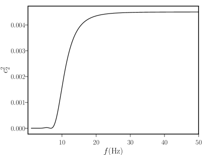
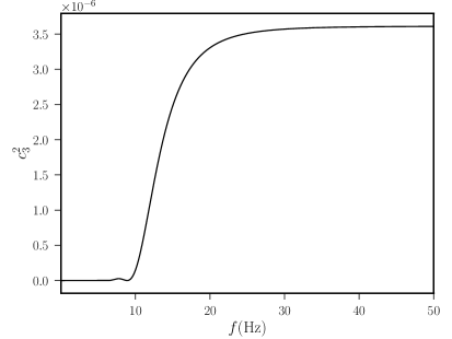
Figure 7: The profiles of $c_{2}^{2}$ and $c_{3}^{2}$ for the profile of Figure 6. We fix $\beta=0.1$.

Let us start focussing on the case $m=2$. The function ${\cal S}_{m}$ reads (we make use of the formulas in Appendix C)

$${\cal S}_{2}\,=\,\sum_{{\cal O}{\cal O}^{\prime}}{\cal R}_{{\cal O}{\cal O}^{\prime}}^{(1,1)}\,=\,c_{2}(f)\,\left(\sum_{\cal O\cal O^{\prime}}v_{\perp}^{a}\,d_{{\cal O}\,ab}\,d^{\,\,\,b}_{{\cal O}^{\prime}\,d}\,v_{\perp}^{d}\right)\,.$$ (5.12)

Here we have included only the contribution due to $c_{2}$, since the additional contribution of $c_{3}$, being subdominant, can be neglected (see Fig 7). The corresponding SNR₂ reads

$${\rm SNR}_{2}=\left(\sqrt{\frac{T}{1{\rm year}}}\times\frac{\Omega_{\rm GW}^{(0)}}{{10^{-12}}}\right)\left(\frac{\Sigma_{\mathcal{O}\mathcal{O^{\prime}}}\,v^{a}_{\perp}\,d_{\mathcal{O}\,ab}\,d_{\mathcal{O^{\prime}}\,d}^{b}\,v_{\perp}^{d}}{\frac{4}{5}\,\Sigma_{\mathcal{O}\mathcal{O^{\prime}}}\,d_{\mathcal{O}\,ab}\,d_{\mathcal{O^{\prime}}}^{ab}}\right)\left(\int_{f_{\rm min}}^{f_{\rm max}}\,{\rm d}f\,\mathcal{A}(f)\right)^{1/2},$$ (5.13)

with

$$\mathcal{A}(f)=c_{2}^{2}(f)\,\left(\frac{\Omega_{\rm GW}(f)}{\Omega_{\rm GW}^{(0)}}\right)^{2}\left(\frac{10^{-12}}{\Sigma_{\rm GW}(f)}\right)^{2},$$ (5.14)

where we use $1$ year$=365.25$ days $=31.56\times 10^{6}$ ${\rm Hz}^{-1}$, and we introduce the quantity

$$\Sigma_{\rm GW}(f)=\frac{4\,\pi^{2}\,f^{3}}{3\,H_{0}^{2}}\left(\frac{N(f)}{\frac{4}{5}\,\Sigma_{\mathcal{O}\mathcal{O^{\prime}}}\,d_{\mathcal{O}\,ab}\,d_{\mathcal{O^{\prime}}}^{ab}}\right)\left(\frac{1}{\sqrt{31.56\times 10^{6}}}\right),$$ (5.15)

which corresponds to the sensitivity curve for the detection of a stochastic background with one year of data collection – see Section IVA of [55], and Figure 14 of [49]. Besides the overall $f^{3}$ and constant factors, this function is defined in terms of the noise correlation $N$ of eq (2.8) (common to all non-null channels, and built in terms of publicly available ET-D specifications  [61]), over the response function for an isotropic background (defined as in eq (3.6) with all $c_{i}$ set to zero), and over the square root of one year expressed in Hz^-1.

The SNR₂ of eq (5.13) is then made of three coefficients, with transparent physical interpretations:

1. The overall square root of the observation time, as expected. We accompany it with the coefficient ${\Omega_{\rm GW}^{(0)}}/{10^{-12}}$, setting the fiducial overall normalization for the SGWB energy density as in Fig 6.

2. A purely geometrical contribution, depending on the orientation of the detector with respect to the projection of the velocity vector normal to the Earth rotation axis.

3. An integral in frequency, which depends on the profile of the SGWB, as well as on the detector specification. The integral is computed over the detectable frequency band of ET. It contains the square of the GW density (see Fig 6) and the square of the Doppler coefficient $c_{2}$ (see Fig 7, left panel), that makes it sensitive to the degree of kinematic anisotropy of the scenario. Finally, it also depends on the square of noise energy density (see eq (5.15)).

For definiteness, in Fig 8 we represent the function ${\cal A}(f)$ of eq (5.14), which appears in the frequency integral in eq (5.13). We notice a very pronounced peak at frequencies around $10$ Hz, nearby the maximal sensitivity of the instrument. It also corresponds to the region where the SGWB changes slope. Notice that the peak is slightly slanted towards high frequencies: we interpret this behaviour to be due to the ‘high-pass’ filter function $c_{2}^{2}$, as commented at the beginning of this subsection.

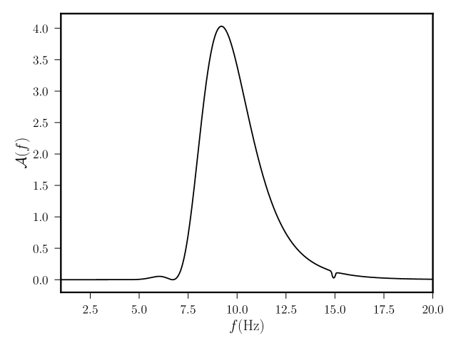
Figure 8: Plot of the integrand function ${\cal A}(f)$ of eq (5.14), computed for the example of Figs. 6, 7. This function has a peak at frequencies around $10$ Hz, in proximity of the region of maximal sensitivity of ET.

The integral over frequencies corresponding to the last factor of eq (5.13) can be numerically computed. We find

$$\left(\int_{1\,{\rm Hz}}^{10^{4}\,{\rm Hz}}\frac{df}{\rm 1\,Hz}\,{\cal A}(f)\right)^{1/2}\,=\,3.66\,.$$ (5.16)

Hence we learn that, if the geometrical second factor of eq (5.13) is of order one, we need an ${\Omega_{\rm GW}^{(0)}}\simeq{10^{-12}}$ for ensuring ${\rm SNR}_{2}>1$. The integral over frequencies in eq (5.16) helps in increasing the prospects of detectability - a feature that has been exploited in the past in the context of power-law sensitivity curves [69] (see also [70] for a recent proposal for the case of broken power-laws).

We now continue with the case $m=4$. The function ${\cal S}_{4}$ results (see Appendix C)

$${\cal S}_{4}\,=\,\sum_{{\cal O}{\cal O}^{\prime}}{\cal R}_{{\cal O}{\cal O}^{\prime}}^{(2,2)}\,=\,\frac{c_{3}}{16}\left(\sum_{\cal O\cal O^{\prime}}\,d_{{\cal O}\,ab}\,d_{{\cal O}^{\prime}\,cd}\,v_{\perp}^{a}\,v_{\perp}^{b}\,v_{\perp}^{c}\,v_{\perp}^{d}\right).$$ (5.17)

In this case, this quantity is insensitive to $c_{2}$: hence it can probe the function $c_{3}$ that – although small – is the only parameter contributing. Proceeding exactly as above, the corresponding SNR₄ reads

$${\rm SNR}_{4}=\left(\sqrt{\frac{T}{1{\rm year}}}\times\frac{\Omega_{\rm GW}^{(0)}}{{10^{-12}}}\right)\left(\frac{\Sigma_{\mathcal{O}\mathcal{O^{\prime}}}\,d_{\mathcal{O}\,ab}\,d_{\mathcal{O^{\prime}}\,cd}\,v_{\perp}^{a}\,v_{\perp}^{b}\,v_{\perp}^{c}\,v_{\perp}^{d}}{\frac{4}{5}\,\Sigma_{\mathcal{O}\mathcal{O^{\prime}}}\,d_{\mathcal{O}\,ab}\,d_{\mathcal{O^{\prime}}}^{ab}}\right)\left(\int_{f_{\rm min}}^{f_{\rm max}}\,{\rm d}f\,\mathcal{B}_{1}(f)\right)^{1/2},$$ (5.18)

with

$$\mathcal{B}_{1}(f)=3.9\times 10^{-3}\times c_{3}^{2}(f)\,\left(\frac{\Omega_{\rm GW}(f)}{\Omega_{\rm GW}^{(0)}}\right)^{2}\left(\frac{10^{-12}}{\Sigma_{\rm GW}(f)}\right)^{2}.$$ (5.19)

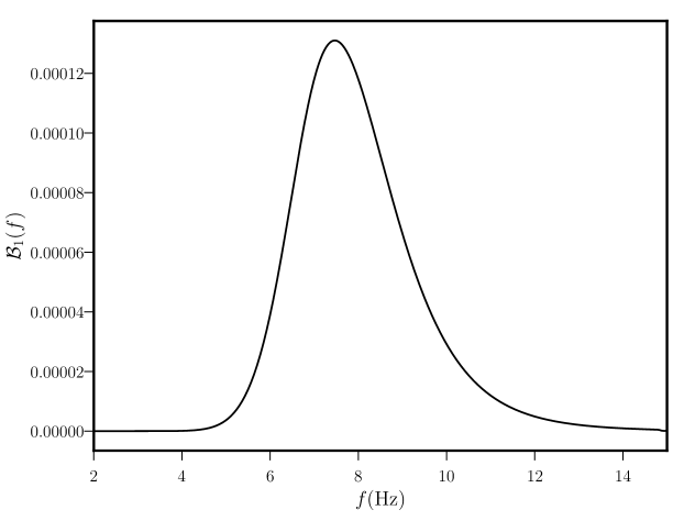
Figure 9: Plot of the function ${\cal B}_{1}(f)$ in eq (5.19), computed for the example of Figures 6, 7.

Again, the profile of the function (see Fig. 9) is peaked at frequencies around the maximal sensitivity of ET, and it is slightly slanted towards the right, because of the ‘high-pass’ behaviour of the weighted function $c_{3}^{2}$. This time, the integral can be numerically computed to be

$$\left(\int_{1\,{\rm Hz}}^{10^{4}\,{\rm Hz}}\frac{df}{\rm 1\,Hz}\,{\cal B}_{1}(f)\right)^{1/2}\,=\,3.96\times 10^{-4}\,,$$ (5.20)

making it harder to detect the effects of $c_{3}$ with respect to $c_{2}$. The remaining cases of $m\neq 2,\,4$ can be treated analogously to these ones, and we do not go through them explicitly.

As a last example, we compute the signal-to-noise ratio ${\rm SNR}_{4}$ for the case of double broken power-law of eq (4.5), that is, the profile with resonance in Fig 4, as discussed in Section 4.3. By making use of eq (3.3), we convert the GW intensity of eq (4.5) into GW energy density. The corresponding profile is

$${\Omega}_{\rm GW}(f)\,=\,{\Omega}_{1}\,\left(\frac{f}{f_{1}}\right)^{\gamma}\left[1+\left(\frac{f}{f_{\star}}\right)^{\frac{1}{\kappa}}\right]^{-\kappa(\gamma+\delta)}+{\Omega}_{2}\,\left(\frac{f}{f_{\rm 2}}\right)^{\gamma_{1}}\left[1+\left(\frac{f}{f_{3}}\right)^{\frac{1}{\kappa_{1}}}\right]^{-\kappa_{1}(\gamma_{1}+\delta_{1})}\,,$$ (5.21)

where ${\Omega}_{1,2}$ are normalization factors, and the meaning and implications of the remaining quantities are discussed after eq (4.5).

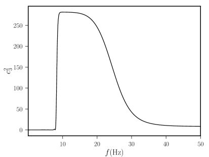
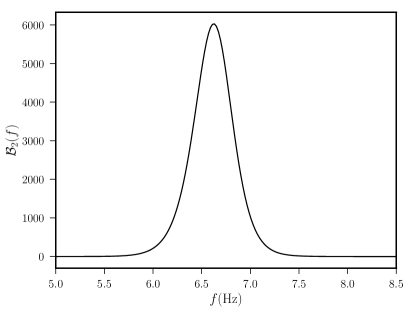
Figure 10: Left panel: The profile of the quantity $c_{3}^{2}$ in the scenario with energy profile (5.21), represented in Fig 4. It is non-vanishing only for a limited range of frequencies. Right panel: The function ${\cal B}_{2}(f)$ of eq (5.23).

We express the formula for the SNR for the case $m=4$ as

$${\rm SNR}_{4}=\left(\sqrt{\frac{T}{1{\rm year}}}\times\frac{\Omega_{\rm GW}^{(0)}}{{10^{-12}}}\right)\left(\frac{\Sigma_{\mathcal{O}\mathcal{O^{\prime}}}\,d_{\mathcal{O}\,ab}\,d_{\mathcal{O^{\prime}}\,cd}\,v_{\perp}^{a}\,v_{\perp}^{b}\,v_{\perp}^{c}\,v_{\perp}^{d}}{\frac{4}{5}\,\Sigma_{\mathcal{O}\mathcal{O^{\prime}}}\,d_{\mathcal{O}\,ab}\,d_{\mathcal{O^{\prime}}}^{ab}}\right)\left(\int_{f_{\rm min}}^{f_{\rm max}}\,{\rm d}f\,\mathcal{B}_{2}(f)\right)^{1/2},$$ (5.22)

with $\Omega_{\rm GW}^{(0)}$ being a ‘fiducial’ reference scale for the amplitude of the SGWB energy density, and

$$\mathcal{B}_{2}(f)=3.9\times 10^{-3}\times c_{3}^{2}(f)\,\left(\frac{\Omega_{\rm GW}(f)}{\Omega_{\rm GW}^{(0)}}\right)^{2}\left(\frac{10^{-12}}{\Sigma_{\rm GW}(f)}\right)^{2}.$$ (5.23)

The function ${\cal B}_{2}(f)$ depends on $c_{3}^{2}$, which assumes large values. The profile of ${\cal B}_{2}(f)$ is peaked for values of frequency at the maximal sensitivity of ET (see Fig. 10). The frequency integral in eq (5.22) can be evaluated to be

$$\left(\int_{1\,{\rm Hz}}^{10^{4}\,{\rm Hz}}\frac{df}{\rm 1\,Hz}\,{\cal B}_{2}(f)\right)^{1/2}\,=\,3.14\times 10^{3}.$$ (5.24)

Apparently, having pronounced resonances or features seems to enhance the detectability of anisotropic signals, a fact pointed out recently in [14].

6 Conclusions

We studied the response function of the Einstein Telescope to kinematic anisotropies of the stochastic gravitational wave background. For the first time we did not assume a factorizable Ansatz for the Doppler effects, nor did we assume the limit of small velocity among frames. We applied our findings to quantitatively study the response functions for three well motivated examples of gravitational wave background profiles: power-law, broken power-law, and models with resonances motivated by primordial black hole scenarios. We then derived the signal- to-noise ratio associated with an optimal estimator for the detection of non-factorizable kinematic anisotropies. We analyzed the signal-to-noise ratio for some representative examples of broken and doubly broken power-law profiles.

Our work can be extended in several directions. First of all, it would be interesting to study further examples of realistic background profiles, to investigate more systematically how Doppler kinematic effects depend on the background profile, and which scenarios lead to higher signal-to-noise ratio and are easier to detect. Also, it would be useful to quantify (as in [47]) corrections to the assumption of negligible vertex distance, as discussed towards the end of section 2, and investigate whether those corrections can be important for specific background profiles.

At the level of applications, the detection and precise measurements of kinematic anisotropies can represent a new indirect avenue for characterizing the properties of the stochastic gravitational wave background, and its sources. Suppose in fact that the yet-to-be detected stochastic background is made of different sources: their possible different speeds with respect to us make a difference in their contributions to Doppler anisotropies, and a measurement of the latter might allow us to distinguish among sources. These and other fascinating questions are left to future work.

Acknowledgments

We are partially funded by the STFC grant ST/T000813/1. For the purpose of open access, the authors have applied a Creative Commons Attribution (CC BY) licence to any Author Accepted Manuscript version arising.

Appendix A Proof of equation (3.6)

The aim of this Appendix is to prove eq (3.6). We write

$${\cal R}_{{\cal O}\,{\cal O}^{\prime}}(f,t,t^{\prime})\,=\,{d^{ab}_{{\cal O}}(t)\,d^{cd}_{{\cal O}^{\prime}}(t)}\,\Gamma_{abcd}(f,\beta,\hat{v})\,,$$ (A.1)

with

$$\Gamma_{abcd}(f,\beta,\hat{v})\,=\,\sum_{\lambda}\int\frac{d^{2}\hat{n}}{4\pi}{\bf P}(f,\,\hat{n})\,{\bf e}_{ab}^{(\lambda)}(\hat{n}){\bf e}_{cd}^{(\lambda)}(\hat{n})\,,$$ (A.2)

and, as in [47], we neglect separation distance among detectors, and ${\bf P}$ is given by eq (3.5). Since it is contracted with the $d^{ab}$’s, we will only be interested in the contributions $\Gamma_{abcd}$ which are traceless along the first and last two indexes. Moreover, $\Gamma_{abcd}$ is symmetric under the interchanges $a\leftrightarrow b$, $c\leftrightarrow d$, $ab\leftrightarrow cd$. We use the identity in Appendix A of [71]:

$$\sum_{\lambda}\,{\bf e}_{ab}^{(\lambda)}(\hat{n}){\bf e}_{cd}^{(\lambda)}(\hat{n}) = \left(\delta_{ac}-\hat{n}_{a}\hat{n}_{c}\right)\left(\delta_{bd}-\hat{n}_{b}\hat{n}_{d}\right)+\left(\delta_{ad}-\hat{n}_{a}\hat{n}_{d}\right)\left(\delta_{bc}-\hat{n}_{b}\hat{n}_{c}\right)$$ (A.3)

$$-\left(\delta_{ab}-\hat{n}_{a}\hat{n}_{b}\right)\left(\delta_{cd}-\hat{n}_{c}\hat{n}_{d}\right)\,.$$

The quantity we are after can be conveniently separated into two parts:

$$\Gamma_{abcd}\,=\,\Gamma_{abcd}^{\rm(iso)}+\Gamma_{abcd}^{\rm(aniso)}\,,$$ (A.4)

with

$$\Gamma_{abcd}^{\rm(iso)} = \sum_{\lambda}\int\frac{d^{2}\hat{n}}{4\pi}\,{\bf e}_{ab}^{(\lambda)}(\hat{n}){\bf e}_{cd}^{(\lambda)}(\hat{n})\,,$$ (A.5)

$$\Gamma_{abcd}^{\rm(aniso)} = \sum_{\lambda}\int\frac{d^{2}\hat{n}}{4\pi}\left({\bf P}-1\right)\,{\bf e}_{ab}^{(\lambda)}(\hat{n}){\bf e}_{cd}^{(\lambda)}(\hat{n})\,.$$ (A.6)

By symmetry considerations, (see e.g. [57]) the isotropic part can only be proportional to the combinations

$$\Gamma_{abcd}^{\rm(iso)}\,=\,{b_{1}}\,\left(\delta_{ac}\delta_{bd}+\delta_{ad}\delta_{bc}\right)+b_{2}\,\delta_{ab}\delta_{cd}\,,$$ (A.7)

where $b_{1,2}$ are functions of frequency. Using identity (A.3), and the fact that $\int{d^{2}\hat{n}}/{4\pi}\,=\,1$, we find that

$$\delta_{cd}\,\delta_{ab}\,\Gamma_{abcd}^{\rm(iso)} = 6\,b_{1}\,+9\,b_{2}\,\,=\,0\,,$$ (A.8)

$$\delta_{bd}\,\delta_{ac}\,\Gamma_{abcd}^{\rm(iso)} = 12\,b_{1}\,+3\,b_{2}\,\,=\,4\,.$$ (A.9)

Hence $b_{1}=2/5$, $b_{2}=-4/15$. The part proportional to $b_{2}$ will vanish upon contractions with the $d^{ab}_{\cal O}$ quantities.

The anisotropic part $\Gamma_{abcd}^{\rm(aniso)}$ can in principle be proportional to the following combinations:

$$\Gamma_{abcd}^{\rm(aniso)} = c_{1}\,\left(\delta_{ac}\delta_{bd}+\delta_{ad}\delta_{bc}\right)+c_{2}\left(\delta_{ac}\hat{v}_{b}\hat{v}_{d}+\delta_{ad}\hat{v}_{b}\hat{v}_{c}+\delta_{bc}\hat{v}_{a}\hat{v}_{d}+\delta_{bd}\hat{v}_{a}\hat{v}_{c}\right)+c_{3}\hat{v}_{a}\hat{v}_{b}\hat{v}_{c}\hat{v}_{d}\noindent$$

$$+ c_{4}\,\delta_{ab}\delta_{cd}+c_{5}\left(\delta_{ab}\hat{v}_{c}\hat{v}_{d}+\delta_{cd}\hat{v}_{a}\hat{v}_{b}\right)\,.$$

Considerations like the ones above lead to the identities

$$c_{1} = \frac{K_{1}}{8}+\frac{3\,K_{2}}{4}+\frac{K_{3}}{8}\,,$$ (A.10)

$$c_{2} = \frac{3\,K_{1}}{8}-\frac{3\,K_{2}}{4}-\frac{5\,K_{3}}{8}\,,$$ (A.11)

$$c_{3} = \frac{3\,K_{1}}{8}-\frac{15\,K_{2}}{4}+\frac{35\,K_{3}}{8}\,,$$ (A.12)

$$c_{4} = \frac{K_{1}}{8}-\frac{5\,K_{2}}{4}+\frac{K_{3}}{8}\,,$$ (A.13)

$$c_{5} = -\frac{5\,K_{1}}{8}+\frac{9\,K_{2}}{4}-\frac{5\,K_{3}}{8}\,.$$ (A.14)

The quantities $K$ are given in eq (LABEL:def_intK) of the main text. They vanish when $\beta=0$.

Assembling the results, we find that the structure of the response function is

$${\cal R}_{{\cal O}\,{\cal O}^{\prime}}(f,t,t^{\prime}) = \frac{4}{5}\left(1+\frac{5}{2}c_{1}\right)\,{d^{ab}_{{\cal O}}(t)\,d_{{\cal O}^{\prime}\,ab}(t)}+4\,c_{2}\,{d^{ab}_{{\cal O}}(t)\,d_{{\cal O}^{\prime}\,bc}(t)}\,{\hat{v}}^{c}\,{\hat{v}}_{a}$$ (A.15)

$$+c_{3}\,\left(\hat{v}^{a}\hat{v}^{b}\,d_{ab\,{\cal O}}(t)\right)\,\left(\hat{v}^{c}\hat{v}^{d}\,d_{cd\,{\cal O}^{\prime}}(t)\right)\,,$$

corresponding to eq (3.6) of the main text.

Appendix B Exact formulas for the power-law case

The aim of this Appendix is to present the general formulas for the coefficients $c_{i}$ for the power-law Ansatz of section 4.1. They are as follows (denoting $\beta_{\pm}\,=\,1\pm\beta$):

$$c_{1} = \frac{\text{$\beta_{-}$}^{\frac{1}{2}-\frac{\alpha}{2}}\text{$\beta_{+}$}^{\frac{1}{2}-\frac{\alpha}{2}}\left(\text{$\beta_{+}$}^{\alpha}-\text{$\beta_{-}$}^{\alpha}\right)}{\alpha(\text{$\beta_{+}$}-\text{$\beta_{-}$})}-1\,,$$ (B.1)

$$c_{2} = \frac{3\alpha^{2}\beta\text{$\beta_{-}$}^{\alpha}(\text{$\beta_{-}$}\text{$\beta_{+}$})^{3/2}-3\alpha^{2}\beta\text{$\beta_{+}$}^{\alpha}(\text{$\beta_{-}$}\text{$\beta_{+}$})^{3/2}-2\alpha(\alpha+1)(\alpha+2)\beta^{3}\text{$\beta_{+}$}(\text{$\beta_{-}$}\text{$\beta_{+}$})^{\alpha/2}}{6\alpha(\text{$\beta_{-}$}\text{$\beta_{+}$})^{\frac{\alpha}{2}}(\alpha+1)(\alpha+2)\beta^{3}\text{$\beta_{+}$}}$$

$$+\frac{6(\beta+1)\text{$\beta_{+}$}^{\alpha}\sqrt{\text{$\beta_{-}$}\text{$\beta_{+}$}}+3\alpha\beta\sqrt{\text{$\beta_{-}$}}\text{$\beta_{+}$}^{\alpha+\frac{3}{2}}(\alpha\text{$\beta_{+}$}+\beta-2)-3\text{$\beta_{+}$}^{3/2}\text{$\beta_{-}$}^{\alpha+\frac{1}{2}}(\alpha\beta(\alpha\text{$\beta_{+}$}+\beta+2)+2)}{6\alpha(\text{$\beta_{-}$}\text{$\beta_{+}$})^{\frac{\alpha}{2}}(\alpha+1)(\alpha+2)\beta^{3}\text{$\beta_{+}$}}$$

$$c_{3} = -\frac{2\alpha(\alpha+1)(\alpha+2)(\alpha+3)(\alpha+4)\beta^{5}(\text{$\beta_{-}$}\text{$\beta_{+}$})^{\alpha/2}}{10(\text{$\beta_{-}$}\text{$\beta_{+}$})^{\frac{\alpha}{2}}\alpha(\alpha+1)(\alpha+2)(\alpha+3)(\alpha+4)\beta^{5}}$$ (B.3)

$$-\frac{5(\alpha\beta((\alpha+1)\beta((\alpha+2)\beta((\alpha+3)\beta+4)+12)+24)+24)\text{$\beta_{-}$}^{\alpha}\sqrt{\text{$\beta_{-}$}\text{$\beta_{+}$}}}{10(\text{$\beta_{-}$}\text{$\beta_{+}$})^{\frac{\alpha}{2}}\alpha(\alpha+1)(\alpha+2)(\alpha+3)(\alpha+4)\beta^{5}}$$

$$+5\frac{(\alpha\beta((\alpha+1)\beta((\alpha+2)\beta((\alpha+3)\beta-4)+12)-24)+24)\text{$\beta_{+}$}^{\alpha}\sqrt{\text{$\beta_{-}$}\text{$\beta_{+}$}}}{10(\text{$\beta_{-}$}\text{$\beta_{+}$})^{\frac{\alpha}{2}}\alpha(\alpha+1)(\alpha+2)(\alpha+3)(\alpha+4)\beta^{5}}\,.$$

These expressions are valid for any $\alpha$ and $0<\beta<1$. Notice that in some specific limits these power-law results formally diverge, and the limits give logarithmic contributions, as in the $\alpha\to-3$ case discussed in the main text.

Appendix C The coefficients ${\cal R}^{(mm^{\prime})}$

We report here the explicit formulas for the coefficients ${\cal R}_{{\cal O}{\cal O}^{\prime}}^{(m,m^{\prime})}$ as discussed in section 5.1. They are as follows:

$${\cal R}_{{\cal O}{\cal O}^{\prime}}^{(0,0)} = \left(\frac{4}{5}+2c_{1}\right)\,d_{{\cal O}\,ab}\,d^{\,\,\,ab}_{{\cal O}^{\prime}}+4\,c_{2}\,v_{\parallel}^{a}\,d_{{\cal O}\,ab}\,d^{\,\,\,b}_{{\cal O}^{\prime}\,d}\,v_{\parallel}^{d}$$ (C.1)

$$+\frac{c_{3}}{4}\,d_{{\cal O}\,ab}\,d_{{\cal O}^{\prime}\,cd}\,\left(v_{\perp}^{a}\,v_{\perp}^{b}+2\,v_{\parallel}^{a}v_{\parallel}^{b}\right)\,\left(v_{\perp}^{c}\,v_{\perp}^{d}+2\,v_{\parallel}^{c}v_{\parallel}^{d}\right)\,,$$

$${\cal R}_{{\cal O}{\cal O}^{\prime}}^{(1,0)} = 2\,c_{2}\,v_{\perp}^{a}\,d_{{\cal O}\,ab}\,d^{\,\,\,b}_{{\cal O}^{\prime}\,d}\,v_{\parallel}^{d}+\frac{c_{3}}{2}\,d_{{\cal O}\,ab}\,d_{{\cal O}^{\prime}\,cd}\,v_{\perp}^{a}\,v_{\parallel}^{b}\,\left(v_{\perp}^{c}\,v_{\perp}^{d}+2\,v_{\parallel}^{c}v_{\parallel}^{d}\right)$$ (C.2)

$${\cal R}_{{\cal O}{\cal O}^{\prime}}^{(2,0)} = \frac{c_{3}}{8}\,d_{{\cal O}\,ab}\,d_{{\cal O}^{\prime}\,cd}\,v_{\perp}^{a}\,v_{\perp}^{b}\,\left(v_{\perp}^{c}\,v_{\perp}^{d}+2\,v_{\parallel}^{c}v_{\parallel}^{d}\right)\,,$$ (C.3)

$${\cal R}_{{\cal O}{\cal O}^{\prime}}^{(1,1)} = c_{2}\,v_{\perp}^{a}\,d_{{\cal O}\,ab}\,d^{\,\,\,b}_{{\cal O}^{\prime}\,d}\,v_{\perp}^{d}+{c_{3}}\,d_{{\cal O}\,ab}\,d_{{\cal O}^{\prime}\,cd}\,v_{\perp}^{a}\,v_{\parallel}^{b}\,v_{\perp}^{c}\,v_{\parallel}^{d}\,,$$ (C.4)

$${\cal R}_{{\cal O}{\cal O}^{\prime}}^{(2,1)} = \frac{c_{3}}{4}\,d_{{\cal O}\,ab}\,d_{{\cal O}^{\prime}\,cd}\,v_{\perp}^{a}\,v_{\perp}^{b}\,v_{\perp}^{c}\,v_{\parallel}^{d}\,,$$ (C.5)

$${\cal R}_{{\cal O}{\cal O}^{\prime}}^{(2,2)} = \frac{c_{3}}{16}\,d_{{\cal O}\,ab}\,d_{{\cal O}^{\prime}\,cd}\,v_{\perp}^{a}\,v_{\perp}^{b}\,v_{\perp}^{c}\,v_{\perp}^{d}\,.$$ (C.6)

The quantities ${\cal R}_{{\cal O}{\cal O}^{\prime}}^{(m,m^{\prime})}$ have the property that ${\cal R}_{{\cal O}{\cal O}^{\prime}}^{(m,m^{\prime})}\,=\,{\cal R}_{{\cal O}^{\prime}{\cal O}}^{(m^{\prime},m)}$.

Appendix D Computation of the SNR_m, and proof of eq (5.9)

The aim of this appendix is to compute the optimal signal-to-noise ratio

$${\text{SNR}}_{m}\,=\,\frac{\langle{\cal C}_{m}\rangle}{\langle{\cal C}^{2}_{m}\rangle^{1/2}}\,,$$ (D.1)

for the quantities defined in section 5. We proceed by first evaluating the numerator, then the denominator.

Evaluating $\langle{\cal C}_{m}\rangle$: For any $m\neq 0$, the stationary noise does not contribute to $\langle{\cal C}_{m}\rangle$. Hence, this key quantity is only sensitive to the anisotropy signal! Collecting results and definitions in the main text, we find that, for non-vanishing index $m$

$$\langle{\cal C}_{m}\rangle = \frac{1}{2\,T}\,\sum_{{\cal O}{\cal O}^{\prime}}\int_{0}^{T}dt\,e^{-2\pi\,im\,\bar{f}_{e}\,t}\int_{-\infty}^{\infty}df\,df^{\prime}\,\tilde{Q}_{{\cal O}{\cal O}^{\prime}}(f)\,\,\int_{t-\tau/2}^{t+\tau/2}dt^{\prime}\,dt^{\prime\prime}\,e^{2\pi i\left(f-f^{\prime}\right)\left(t^{\prime}-t^{\prime\prime}\right)}{\cal R}_{{\cal O}{\cal O}^{\prime}}(f^{\prime},t^{\prime\prime},t^{\prime})\,{\cal I}(f^{\prime})\,,$$ (D.2)

$$= \frac{1}{2\,T}\,\sum_{{\cal O}{\cal O}^{\prime}}\int_{0}^{T}dt\,e^{-2\pi im\,{\bar{f}}_{e}\,t}\int_{-\infty}^{\infty}df\,df^{\prime}\,\tilde{Q}_{{\cal O}{\cal O}^{\prime}}(f)\,\,{\cal I}(f^{\prime})$$

$$\times\sum_{m^{\prime}m^{\prime\prime}}\,\int_{t-\tau/2}^{t+\tau/2}dt^{\prime}\,dt^{\prime\prime}\,e^{2\pi it^{\prime}\left(f-f^{\prime}+m^{\prime}{\bar{f}}_{e}\right)}\,e^{-2\pi it^{\prime\prime}\left(f-f^{\prime}-m^{\prime\prime}{\bar{f}}_{e}\right)}\,{\cal R}_{{\cal O}{\cal O}^{\prime}}^{(m^{\prime}m^{\prime\prime})}(f^{\prime})\,.$$

To handle the nested integrals, we start performing the time integrals along $t^{\prime},t^{\prime\prime}$.

We use the definition of finite-size $\delta$-function

$$\int_{t-\tau/2}^{t+\tau/2}dt^{\prime}\,e^{2\pi it^{\prime}\left(f^{\prime}-f^{\prime\prime}+m^{\prime}{\bar{f}}_{e}\right)}\,=\,\delta_{\tau}\left(f^{\prime}-f^{\prime\prime}+m^{\prime}{\bar{f}}_{e}\right)\,e^{-2i\pi\,t\,\left(f^{\prime}-f^{\prime\prime}+m^{\prime}\,{\bar{f}}_{e}\right)}\,,$$ (D.3)

with $\delta_{\tau}\left(x\right)$ given by

$$\delta_{\tau}\left(x\right)\,\equiv\,\frac{\sin{(\pi\,x\,\tau)}}{\pi x}\hskip 28.45274pt,\hskip 28.45274pt\lim_{\tau\to\infty}\,\delta_{\tau}\left(x\right)\,=\,\delta_{D}\left(x\right)\,,$$ (D.4)

and $\delta_{D}$ being the Dirac delta. Then we get the expression

$$\langle{\cal C}_{m}\rangle = \frac{1}{2\,T}\,\sum_{{\cal O}{\cal O}^{\prime}}\,\sum_{m^{\prime}m^{\prime\prime}}\int_{0}^{T}dt\,e^{-2\pi im\,{\bar{f}}_{e}\,t}\int_{-\infty}^{\infty}df\,df^{\prime}\,\tilde{Q}_{{\cal O}{\cal O}^{\prime}}(f)\,\,{\cal I}(f^{\prime}){\cal R}_{{\cal O}{\cal O}^{\prime}}^{(m^{\prime}m^{\prime\prime})}(f^{\prime})$$ (D.5)

$$\times\delta_{\tau}\left(f-f^{\prime}+m^{\prime}{\bar{f}}_{e}\right)\,\delta_{\tau}\left(f-f^{\prime}-m^{\prime\prime}{\bar{f}}_{e}\right)\,e^{2i\pi\,t\,\left(m^{\prime}+m^{\prime\prime}\right)\,{\bar{f}}_{e}}\,.$$

Since ${\bar{f}}_{e}$ is much smaller than the frequency $f$ of GW, we can neglect the $m\,{\bar{f}}_{e}$ contributions in the argument of the $\delta_{\tau}$ functions. Moreover, $\tau$ is much longer than the inverse of GW frequencies. Hence we can treat one of the $\delta_{\tau}$ as Dirac delta-function $\delta_{D}$, and obtain

$$\langle{\cal C}_{m}\rangle = \frac{\tau}{2}\,\sum_{{\cal O}{\cal O}^{\prime}}\,\int_{-\infty}^{\infty}df\,\tilde{Q}_{{\cal O}{\cal O}^{\prime}}(f)\,{\cal S}_{{\cal O}{\cal O}^{\prime}}(f)\,{\cal I}(f),$$ (D.6)

for the numerator of eq (D.1), with

$${\cal S}^{(m)}_{{\cal O}{\cal O}^{\prime}}(f)\,=\,\sum_{m^{\prime},m^{\prime\prime}=-2}^{2}\,\delta_{K}(m-m^{\prime}-m^{\prime\prime}){\cal R}_{{\cal O}{\cal O}^{\prime}}^{(m^{\prime},\,m^{\prime\prime})}(f)\,,$$ (D.7)

and $\delta_{K}$ being the Kronecker delta.

Evaluating $\langle{\cal C}^{2}_{m}\rangle^{1/2}$: To evaluate the denominator of eq (D.1), we work under the hypothesis of noise-domination in eq (2.7), and compute the variance of the noise. The steps are very similar to the previous ones, and already carried out in [47], section 3.2. We report the result of the calculation:

$${\langle{\cal C}^{2}_{m}\rangle}\,=\,\frac{\tau^{2}}{4\,T}\,\sum_{{\cal O}{\cal O}^{\prime}}\,\int_{-\infty}^{\infty}df\,|\tilde{Q}_{{\cal O}{\cal O}^{\prime}}(f)|^{2}\,{N}_{{\cal O}}(f)\,{N}_{{\cal O}^{\prime}}(f)\,.$$ (D.8)

We refer the reader to [47] for details.

Estimating the optimal ${\text{SNR}}_{m}$. We now collect the results, and assume that the detector noise ${N}_{{\cal O}}\,=\,{N}$ is the same for all the non-null channels. The expression for the SNR is obtained by combining eqs (D.6) and (D.8):

$${\text{SNR}}_{m} = \sqrt{T}\,\frac{\sum_{{\cal O}{\cal O}^{\prime}}\int_{-\infty}^{\infty}df\,\tilde{Q}_{{\cal O}{\cal O}^{\prime}}(f)\,{\cal S}_{{\cal O}{\cal O}^{\prime}}(f)\,{\cal I}(f)}{\left(\int_{-\infty}^{\infty}df\,\sum_{{\cal O}{\cal O}^{\prime}}|\tilde{Q}_{{\cal O}{\cal O}^{\prime}}(f)|^{2}\,N^{2}(f)\right)^{1/2}}\,,$$ (D.9)

$$= \sqrt{2T}\,\frac{\sum_{{\cal O}{\cal O}^{\prime}}\int_{0}^{\infty}df\,\tilde{Q}_{{\cal O}{\cal O}^{\prime}}(f)\,{\cal S}_{{\cal O}{\cal O}^{\prime}}(f)\,{\cal I}(f)}{\left(\int_{0}^{\infty}df\,\sum_{{\cal O}{\cal O}^{\prime}}|\tilde{Q}_{{\cal O}{\cal O}^{\prime}}(f)|^{2}\,N^{2}(f)\right)^{1/2}}\,,$$

where in the second line we perform an integration only over positive frequencies (hence the $\sqrt{2}$ factor in front). We determine the optimal value for the filter $\tilde{Q}_{{\cal O}{\cal O}^{\prime}}(f)$, using standard techniques based on Wiener filtering [56]. We introduce a positive-definite scalar product $\left[\dots\right]$, defined as:

$$\left[A_{{\cal O}{\cal O}^{\prime}}(f),\,B_{{\cal O}{\cal O}^{\prime}}(f)\right]\,\equiv\,\,\sum_{{\cal O}{\cal O}^{\prime}}\int_{0}^{\infty}df\,A^{*}_{{\cal O}{\cal O}^{\prime}}(f)\,B_{{\cal O}{\cal O}^{\prime}}(f)\,N^{2}(f)\,.$$ (D.10)

Using this scalar product, we re-express (D.9) as

$${\text{SNR}}_{m}\,=\,\sqrt{2T}\,\frac{\left[\tilde{Q}_{{\cal O}{\cal O}^{\prime}}(f),\,{\cal S}_{{\cal O}{\cal O}^{\prime}}(f)\,{\cal I}(f)/N^{2}(f)\right]}{\left[\tilde{Q}_{{\cal O}{\cal O}^{\prime}}(f),\tilde{Q}_{{\cal O}{\cal O}^{\prime}}(f)\right]^{1/2}}\,.$$ (D.11)

This quantity is maximised choosing a filter $\tilde{Q}_{{\cal O}{\cal O}^{\prime}}(f)\,=\,{\cal S}_{{\cal O}{\cal O}^{\prime}}(f)\,{\cal I}(f)/N^{2}(f)$. Using it, the optimal signal-to-noise ratio results

$${\text{SNR}}_{m}\,=\,\sqrt{2T}\,\left(\int_{0}^{\infty}df\,\left|\sum_{{\cal O}{\cal O}^{\prime}}\,{\cal S}^{(m)}_{{\cal O}{\cal O}^{\prime}}(f)\,\,\frac{{\cal I}(f)}{N(f)}\right|^{2}\right)^{1/2}\,,$$ (D.12)

hence demonstrating eq (5.9).

References

- [1] A. I. Renzini, B. Goncharov, A. C. Jenkins, and P. M. Meyers, “Stochastic Gravitational-Wave Backgrounds: Current Detection Efforts and Future Prospects,” Galaxies 10 no. 1, (2022) 34, arXiv:2202.00178 [gr-qc].
- [2] S. Olmez, V. Mandic, and X. Siemens, “Anisotropies in the Gravitational-Wave Stochastic Background,” JCAP 07 (2012) 009, arXiv:1106.5555 [astro-ph.CO].
- [3] S. Kuroyanagi, K. Takahashi, N. Yonemaru, and H. Kumamoto, “Anisotropies in the gravitational wave background as a probe of the cosmic string network,” Phys. Rev. D 95 no. 4, (2017) 043531, arXiv:1604.00332 [astro-ph.CO].
- [4] G. Cusin, C. Pitrou, and J.-P. Uzan, “Anisotropy of the astrophysical gravitational wave background: Analytic expression of the angular power spectrum and correlation with cosmological observations,” Phys. Rev. D 96 no. 10, (2017) 103019, arXiv:1704.06184 [astro-ph.CO].
- [5] A. C. Jenkins and M. Sakellariadou, “Anisotropies in the stochastic gravitational-wave background: Formalism and the cosmic string case,” Phys. Rev. D 98 no. 6, (2018) 063509, arXiv:1802.06046 [astro-ph.CO].
- [6] G. Cusin, I. Dvorkin, C. Pitrou, and J.-P. Uzan, “First predictions of the angular power spectrum of the astrophysical gravitational wave background,” Phys. Rev. Lett. 120 (2018) 231101, arXiv:1803.03236 [astro-ph.CO].
- [7] A. C. Jenkins, M. Sakellariadou, T. Regimbau, and E. Slezak, “Anisotropies in the astrophysical gravitational-wave background: Predictions for the detection of compact binaries by LIGO and Virgo,” Phys. Rev. D 98 no. 6, (2018) 063501, arXiv:1806.01718 [astro-ph.CO].
- [8] R.-G. Cai, Z.-K. Guo, and J. Liu, “A New Picture of Cosmic String Evolution and Anisotropic Stochastic Gravitational-Wave Background,” arXiv:2112.10131 [astro-ph.CO].
- [9] M. Geller, A. Hook, R. Sundrum, and Y. Tsai, “Primordial Anisotropies in the Gravitational Wave Background from Cosmological Phase Transitions,” Phys. Rev. Lett. 121 no. 20, (2018) 201303, arXiv:1803.10780 [hep-ph].
- [10] C. Pitrou, G. Cusin, and J.-P. Uzan, “Unified view of anisotropies in the astrophysical gravitational-wave background,” Phys. Rev. D 101 no. 8, (2020) 081301, arXiv:1910.04645 [astro-ph.CO].
- [11] G. Capurri, A. Lapi, C. Baccigalupi, L. Boco, G. Scelfo, and T. Ronconi, “Intensity and anisotropies of the stochastic gravitational wave background from merging compact binaries in galaxies,” JCAP 11 (2021) 032, arXiv:2103.12037 [gr-qc].
- [12] E. Dimastrogiovanni, M. Fasiello, A. Malhotra, P. D. Meerburg, and G. Orlando, “Testing the early universe with anisotropies of the gravitational wave background,” JCAP 02 no. 02, (2022) 040, arXiv:2109.03077 [astro-ph.CO].
- [13] E. Dimastrogiovanni, M. Fasiello, and L. Pinol, “Primordial Stochastic Gravitational Wave Background Anisotropies: in-in Formalization and Applications,” arXiv:2203.17192 [astro-ph.CO].
- [14] E. Dimastrogiovanni, M. Fasiello, A. Malhotra, and G. Tasinato, “Enhancing gravitational wave anisotropies with peaked scalar sources,” arXiv:2205.05644 [astro-ph.CO].
- [15] V. Alba and J. Maldacena, “Primordial gravity wave background anisotropies,” JHEP 03 (2016) 115, arXiv:1512.01531 [hep-th].
- [16] C. R. Contaldi, “Anisotropies of Gravitational Wave Backgrounds: A Line Of Sight Approach,” Phys. Lett. B 771 (2017) 9–12, arXiv:1609.08168 [astro-ph.CO].
- [17] N. Bartolo, D. Bertacca, S. Matarrese, M. Peloso, A. Ricciardone, A. Riotto, and G. Tasinato, “Anisotropies and non-Gaussianity of the Cosmological Gravitational Wave Background,” Phys. Rev. D 100 no. 12, (2019) 121501, arXiv:1908.00527 [astro-ph.CO].
- [18] N. Bartolo, D. Bertacca, S. Matarrese, M. Peloso, A. Ricciardone, A. Riotto, and G. Tasinato, “Characterizing the cosmological gravitational wave background: Anisotropies and non-Gaussianity,” Phys. Rev. D 102 no. 2, (2020) 023527, arXiv:1912.09433 [astro-ph.CO].
- [19] D. Bertacca, A. Ricciardone, N. Bellomo, A. C. Jenkins, S. Matarrese, A. Raccanelli, T. Regimbau, and M. Sakellariadou, “Projection effects on the observed angular spectrum of the astrophysical stochastic gravitational wave background,” Phys. Rev. D 101 no. 10, (2020) 103513, arXiv:1909.11627 [astro-ph.CO].
- [20] N. Bartolo, D. Bertacca, V. De Luca, G. Franciolini, S. Matarrese, M. Peloso, A. Ricciardone, A. Riotto, and G. Tasinato, “Gravitational wave anisotropies from primordial black holes,” JCAP 02 (2020) 028, arXiv:1909.12619 [astro-ph.CO].
- [21] L. Valbusa Dall’Armi, A. Ricciardone, N. Bartolo, D. Bertacca, and S. Matarrese, “Imprint of relativistic particles on the anisotropies of the stochastic gravitational-wave background,” Phys. Rev. D 103 no. 2, (2021) 023522, arXiv:2007.01215 [astro-ph.CO].
- [22] V. Domcke, R. Jinno, and H. Rubira, “Deformation of the gravitational wave spectrum by density perturbations,” JCAP 06 (2020) 046, arXiv:2002.11083 [astro-ph.CO].
- [23] LISA Cosmology Working Group Collaboration, N. Bartolo et al., “Probing Anisotropies of the Stochastic Gravitational Wave Background with LISA,” arXiv:2201.08782 [astro-ph.CO].
- [24] G. Cusin and G. Tasinato, “Doppler boosting the stochastic gravitational wave background,” JCAP 08 no. 08, (2022) 036, arXiv:2201.10464 [astro-ph.CO].
- [25] LISA Cosmology Working Group Collaboration, P. Auclair et al., “Cosmology with the Laser Interferometer Space Antenna,” arXiv:2204.05434 [astro-ph.CO].
- [26] L. V. Dall’Armi, A. Ricciardone, and D. Bertacca, “The Dipole of the Astrophysical Gravitational-Wave Background,” arXiv:2206.02747 [astro-ph.CO].
- [27] A. K.-W. Chung, A. C. Jenkins, J. D. Romano, and M. Sakellariadou, “Targeted search for the kinematic dipole of the gravitational-wave background,” arXiv:2208.01330 [gr-qc].
- [28] G. F. Smoot, M. V. Gorenstein, and R. A. Muller, “Detection of Anisotropy in the Cosmic Black Body Radiation,” Phys. Rev. Lett. 39 (1977) 898.
- [29] A. Kogut et al., “Dipole anisotropy in the COBE DMR first year sky maps,” Astrophys. J. 419 (1993) 1, arXiv:astro-ph/9312056.
- [30] WMAP Collaboration, C. L. Bennett et al., “First year Wilkinson Microwave Anisotropy Probe (WMAP) observations: Preliminary maps and basic results,” Astrophys. J. Suppl. 148 (2003) 1–27, arXiv:astro-ph/0302207.
- [31] Planck Collaboration, N. Aghanim et al., “Planck 2013 results. XXVII. Doppler boosting of the CMB: Eppur si muove,” Astron. Astrophys. 571 (2014) A27, arXiv:1303.5087 [astro-ph.CO].
- [32] C. Caprini and D. G. Figueroa, “Cosmological Backgrounds of Gravitational Waves,” Class. Quant. Grav. 35 no. 16, (2018) 163001, arXiv:1801.04268 [astro-ph.CO].
- [33] T. Regimbau, “The astrophysical gravitational wave stochastic background,” Res. Astron. Astrophys. 11 (2011) 369–390, arXiv:1101.2762 [astro-ph.CO].
- [34] B. Allen and A. C. Ottewill, “Detection of anisotropies in the gravitational wave stochastic background,” Phys. Rev. D 56 (1997) 545–563, arXiv:gr-qc/9607068.
- [35] N. J. Cornish, “Mapping the gravitational wave background,” Class. Quant. Grav. 18 (2001) 4277–4292, arXiv:astro-ph/0105374.
- [36] C. Ungarelli and A. Vecchio, “Studying the anisotropy of the gravitational wave stochastic background with LISA,” Phys. Rev. D 64 (2001) 121501, arXiv:astro-ph/0106538.
- [37] N. Seto and A. Cooray, “LISA measurement of gravitational wave background anisotropy: Hexadecapole moment via a correlation analysis,” Phys. Rev. D 70 (2004) 123005, arXiv:astro-ph/0403259.
- [38] H. Kudoh and A. Taruya, “Probing anisotropies of gravitational-wave backgrounds with a space-based interferometer: Geometric properties of antenna patterns and their angular power,” Phys. Rev. D 71 (2005) 024025, arXiv:gr-qc/0411017.
- [39] A. Taruya and H. Kudoh, “Probing anisotropies of gravitational-wave backgrounds with a space-based interferometer. II. Perturbative reconstruction of a low-frequency skymap,” Phys. Rev. D 72 (2005) 104015, arXiv:gr-qc/0507114.
- [40] A. Taruya, “Probing anisotropies of gravitational-wave backgrounds with a space-based interferometer III: Reconstruction of a high-frequency skymap,” Phys. Rev. D 74 (2006) 104022, arXiv:gr-qc/0607080.
- [41] E. Thrane, S. Ballmer, J. D. Romano, S. Mitra, D. Talukder, S. Bose, and V. Mandic, “Probing the anisotropies of a stochastic gravitational-wave background using a network of ground-based laser interferometers,” Phys. Rev. D 80 (2009) 122002, arXiv:0910.0858 [astro-ph.IM].
- [42] C. M. F. Mingarelli, T. Sidery, I. Mandel, and A. Vecchio, “Characterizing gravitational wave stochastic background anisotropy with pulsar timing arrays,” Phys. Rev. D 88 no. 6, (2013) 062005, arXiv:1306.5394 [astro-ph.HE].
- [43] S. R. Taylor and J. R. Gair, “Searching For Anisotropic Gravitational-wave Backgrounds Using Pulsar Timing Arrays,” Phys. Rev. D 88 (2013) 084001, arXiv:1306.5395 [gr-qc].
- [44] J. Baker et al., “High angular resolution gravitational wave astronomy,” Exper. Astron. 51 no. 3, (2021) 1441–1470, arXiv:1908.11410 [astro-ph.HE].
- [45] J. D. Romano and N. J. Cornish, “Detection methods for stochastic gravitational-wave backgrounds: a unified treatment,” Living Rev. Rel. 20 no. 1, (2017) 2, arXiv:1608.06889 [gr-qc].
- [46] N. Bartolo et al., “Science with the space-based interferometer LISA. IV: Probing inflation with gravitational waves,” JCAP 12 (2016) 026, arXiv:1610.06481 [astro-ph.CO].
- [47] G. Mentasti and M. Peloso, “ET sensitivity to the anisotropic Stochastic Gravitational Wave Background,” JCAP 03 (2021) 080, arXiv:2010.00486 [astro-ph.CO].
- [48] M. Punturo et al., “The Einstein Telescope: A third-generation gravitational wave observatory,” Class. Quant. Grav. 27 (2010) 194002.
- [49] M. Maggiore et al., “Science Case for the Einstein Telescope,” JCAP 03 (2020) 050, arXiv:1912.02622 [astro-ph.CO].
- [50] S. Kuroyanagi, T. Chiba, and T. Takahashi, “Probing the Universe through the Stochastic Gravitational Wave Background,” JCAP 11 (2018) 038, arXiv:1807.00786 [astro-ph.CO].
- [51] K. N. Ananda, C. Clarkson, and D. Wands, “The Cosmological gravitational wave background from primordial density perturbations,” Phys. Rev. D 75 (2007) 123518, arXiv:gr-qc/0612013.
- [52] D. Baumann, P. J. Steinhardt, K. Takahashi, and K. Ichiki, “Gravitational Wave Spectrum Induced by Primordial Scalar Perturbations,” Phys. Rev. D 76 (2007) 084019, arXiv:hep-th/0703290.
- [53] R. Saito and J. Yokoyama, “Gravitational wave background as a probe of the primordial black hole abundance,” Phys. Rev. Lett. 102 (2009) 161101, arXiv:0812.4339 [astro-ph]. [Erratum: Phys.Rev.Lett. 107, 069901 (2011)].
- [54] R. Saito and J. Yokoyama, “Gravitational-Wave Constraints on the Abundance of Primordial Black Holes,” Prog. Theor. Phys. 123 (2010) 867–886, arXiv:0912.5317 [astro-ph.CO]. [Erratum: Prog.Theor.Phys. 126, 351–352 (2011)].
- [55] T. L. Smith and R. Caldwell, “LISA for Cosmologists: Calculating the Signal-to-Noise Ratio for Stochastic and Deterministic Sources,” Phys. Rev. D 100 no. 10, (2019) 104055, arXiv:1908.00546 [astro-ph.CO].
- [56] M. Maggiore, Gravitational Waves. Vol. 1: Theory and Experiments. Oxford Master Series in Physics. Oxford University Press, 2007.
- [57] B. Allen and J. D. Romano, “Detecting a stochastic background of gravitational radiation: Signal processing strategies and sensitivities,” Phys. Rev. D 59 (1999) 102001, arXiv:gr-qc/9710117.
- [58] M. Tinto, F. B. Estabrook, and J. W. Armstrong, “Time delay interferometry for LISA,” Phys. Rev. D 65 (2002) 082003.
- [59] M. Tinto and S. V. Dhurandhar, “TIME DELAY,” Living Rev. Rel. 8 (2005) 4, arXiv:gr-qc/0409034.
- [60] M. Vallisneri, “Geometric time delay interferometry,” Phys. Rev. D 72 (2005) 042003, arXiv:gr-qc/0504145. [Erratum: Phys.Rev.D 76, 109903 (2007)].
- [61] S. Hild et al., “Sensitivity Studies for Third-Generation Gravitational Wave Observatories,” Class. Quant. Grav. 28 (2011) 094013, arXiv:1012.0908 [gr-qc].
- [62] L. Sampson, N. J. Cornish, and S. T. McWilliams, “Constraining the Solution to the Last Parsec Problem with Pulsar Timing,” Phys. Rev. D 91 no. 8, (2015) 084055, arXiv:1503.02662 [gr-qc].
- [63] A. R. Kaiser, N. S. Pol, M. A. McLaughlin, S. Chen, J. S. Hazboun, L. Z. Kelley, J. Simon, S. R. Taylor, S. J. Vigeland, and C. A. Witt, “Disentangling Multiple Stochastic Gravitational Wave Background Sources in PTA Datasets,” arXiv:2208.02307 [astro-ph.CO].
- [64] G. Domènech, “Scalar Induced Gravitational Waves Review,” Universe 7 no. 11, (2021) 398, arXiv:2109.01398 [gr-qc].
- [65] J. R. Espinosa, D. Racco, and A. Riotto, “A Cosmological Signature of the SM Higgs Instability: Gravitational Waves,” JCAP 09 (2018) 012, arXiv:1804.07732 [hep-ph].
- [66] K. Kohri and T. Terada, “Semianalytic calculation of gravitational wave spectrum nonlinearly induced from primordial curvature perturbations,” Phys. Rev. D 97 no. 12, (2018) 123532, arXiv:1804.08577 [gr-qc].
- [67] S. Pi and M. Sasaki, “Gravitational Waves Induced by Scalar Perturbations with a Lognormal Peak,” JCAP 09 (2020) 037, arXiv:2005.12306 [gr-qc].
- [68] C. Caprini, D. G. Figueroa, R. Flauger, G. Nardini, M. Peloso, M. Pieroni, A. Ricciardone, and G. Tasinato, “Reconstructing the spectral shape of a stochastic gravitational wave background with LISA,” JCAP 11 (2019) 017, arXiv:1906.09244 [astro-ph.CO].
- [69] E. Thrane and J. D. Romano, “Sensitivity curves for searches for gravitational-wave backgrounds,” Phys. Rev. D 88 no. 12, (2013) 124032, arXiv:1310.5300 [astro-ph.IM].
- [70] D. Chowdhury, G. Tasinato, and I. Zavala, “The rise of the primordial tensor spectrum from an early scalar-tensor epoch,” JCAP 08 no. 08, (2022) 010, arXiv:2204.10218 [gr-qc].
- [71] V. Domcke, J. Garcia-Bellido, M. Peloso, M. Pieroni, A. Ricciardone, L. Sorbo, and G. Tasinato, “Measuring the net circular polarization of the stochastic gravitational wave background with interferometers,” JCAP 05 (2020) 028, arXiv:1910.08052 [astro-ph.CO].