An extensive numerical benchmark study of deterministic vs. stochastic derivative-free global optimization algorithms

Abstract

Research in derivative-free global optimization is under active development, and many solution techniques are available today. Therefore, the experimental comparison of previous and emerging algorithms must be kept up to date. This paper considers the solution to the bound-constrained, possibly black-box global optimization problem. It compares $64$ derivative-free deterministic algorithms against classic and state-of-the-art stochastic solvers. Among deterministic ones, a particular emphasis is on DIRECT-type, where, in recent years, significant progress has been made. A set of $800$ test problems generated by the well-known GKLS generator and $397$ traditional test problems from DIRECTGOLib v1.2 collection are utilized in a computational study. More than $239,400$ solver runs were carried out, requiring more than $531$ days of single CPU time to complete them. It has been found that deterministic algorithms perform excellently on GKLS-type and low-dimensional problems, while stochastic algorithms have shown to be more efficient in higher dimensions.

1 Introduction

Optimization methods are continuously used today to improve and optimize business processes in various areas of human activity and industry. In this paper, we consider a general single-objective optimization problem, which can be formally stated as:

$$\min_{\mathbf{x}\in D} f(\mathbf{x})$$ (1)

where $f:\mathbb{R}^{n}\rightarrow\mathbb{R}$ is a Lipschitz-continuous objective function (with an unknown Lipschitz constant), and $\mathbf{x}\in\mathbb{R}^{n}$ is the input vector of control variables. We assume that $f$ can be computed at any point of the feasible region, which is an $n$-dimensional hyper-rectangle

$$D=[\mathbf{a},\mathbf{b}]=\{\mathbf{x}\in\mathbb{R}^{n}:a_{j}\leq x_{j}\leq b_{j},j=1,\dots,n\}.$$

Moreover, $f$ can be non-linear, multi-modal, non-convex, and non-differentiable.

It is common practice in many fields of science and engineering to optimize a function derived from an experiment or a highly complex computer simulation. In addition, as the scale and complexity of applications increase, objective function evaluations become more expensive. Such situations make derivatives either impossible or impractical to calculate. Thus, this paper also assumes that the objective function is potentially “black-box.” Therefore, any analytical information about the objective function is unknown, and optimization solvers can only use the objective function values.

Numerical methods are commonly applied to solve “black-box” problems Zhigljavsky2008:book ; William2007 . The development of derivative-free optimization algorithms has a long history in the field of optimization, dating back to the work of Hooke and Jeeves Hooke1961 with their famous “direct search” approach. After several years of work, derivative-free techniques have lost popularity in the mathematical optimization community, as some of them converge slowly or even can not guarantee global convergence Xi2020 . However, in recent decades, derivative-free optimization has regained interest due to the growing number of applications and has attracted much attention from the optimization community Ezugwu2021 ; Jones2021 . Our collected data from the Web of Science (WoS) shows more than $1800$ publications related to derivative-free optimization (see Table 1).

Table 1: The number of publications related to derivative-free optimization (in WoS database).

Document Type	Record Count	Percentage
Articles	$1,064$	$57.64\%$
Proceedings Paper	$725$	$39.27\%$
Review Articles	$27$	$1.46\%$
Book Chapters	$29$	$1.57\%$
Book	$1$	$0.05\%$

The cumulative number of publications from $1991$ to $2021$ is plotted in Fig. 1. The number of “derivative-free” related publications grows each year consistently. Naturally, the number will be significantly higher in some other databases such as Google Scholar.

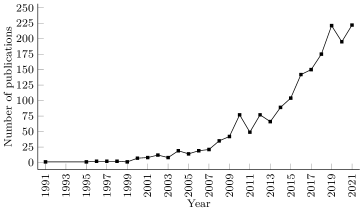
Figure 1: The number of publications related to derivative-free optimization from $1990$ to $2021$ (in WoS database).

Choosing the proper optimization algorithm (solver) for a solution to global optimization problems is complicated. First, the user needs to know how different solvers perform compared to other algorithms on an extensive set of different test and possibly (related) practical problems. The choice is further complicated because global optimization techniques are different. Stochastic nature-inspired global optimization algorithms incorporate probabilistic (stochastic) elements. The convergence is guaranteed only in a probabilistic sense, i.e., in infinite time, a global optimum will be found with probability one Zhigljavsky2008:book . Deterministic algorithms can guarantee that after a finite time a global optimum will be found within small prescribed tolerances Floudas1999book ; Horst1996:book .

Identification of the most effective derivative-free global optimization algorithms is a challenging task. Typically, the authors of new algorithms limit themselves to small efficiency studies against only a few related algorithms (see, e.g., Abdollahzadeh2021 ; Alsattar2020 ; Azizi2021 ; Stripinis2018a ; Liu2015 ). Therefore, the complete picture of the algorithm’s performance across state-of-the-art algorithms is unclear. Unfortunately, detailed comparative analyzes in the field are rare, and there is a constant need to update them by including recent algorithms.

1.1 Related surveys and benchmarks

Table 2 summarizes related works devoted to solving derivative-free global optimization problems. Here, the first three columns give the source of the research, the year of publication, and the impact expressed as the total number of citations (according to Google Scholar). The fourth column indicates the total number of solvers, while the fifth shows the total number of test problems used in the experimental studies. The last two columns give the range of the dimension and the function evaluation budget.

Most published surveys (see, e.g., Mongeau2000 ; Auger2009 ; Pham2011 ; Stripinis2021c ; Kvasov2018 ; Liu2019 ) are limited to relatively small-dimensional test problems. The largest number of derivative-free global optimization solvers was investigated in our recent publication Stripinis2021c , where the new DIRECTGO toolbox was introduced. Nevertheless, this paper considered only DIRECT-type Jones1993 algorithms. However, the most extensive study of derivative-free solvers was carried out in Rios2013 and currently has the most significant impact. The study was carried out using only a limited budget of objective function evaluations, typical for expensive global optimization problems. Since then, the number of new derivative-free optimization solvers significantly increased, and it is not clear whether the best-performing algorithms are still the best?

Table 2: History of derivative-free global optimization numerical studies

Source	Year	Impact	Number of		Range	Evaluation
			solvers	problems	of $n$	budget
Mongeau et al. Mongeau2000	$2000$	$80$	$6$	$11$	$1-20$	$700-30,000$
Hansen et al. Hansen2010	$2010$	$411$	$31$	$120$	$2-40$	$100,000,000n$
Auger et al. Auger2009	$2011$	$98$	$5$	$3$	$10-40$	$10,000,000$
Pham et al. Pham2011	$2011$	$58$	$5$	$16$	$20$	$100,000$
Rios et al. Rios2013	$2013$	$1,260$	$22$	$502$	$1-300$	$2,500$
Kvasov et al. Kvasov2018	$2018$	$78$	$13$	$134$	$1$	$10,000$
Liu et al. Liu2019	$2019$	$17$	$27$	$126$	$1$	$1,000$
Stripinis et al. Stripinis2021c	$2022$	$1$	$39$	$128$	$2-15$	$2,000,000$
This paper	$2022$	$0$	$64$	$1,197$	$2-100$	$2,500-500,000$

1.2 Main contributions

The main contributions of this research are the following:

• The largest set of solvers ($64$) considered in the experimental study of derivative-free global optimization.

• Large and diverse benchmark pool ($1,197$) consisting of:

  • The GKLS-type multi-modal box-constrained “black-box” global optimization problems Gaviano2003 (recently extended to generally-constrained problems Sergeyev2021gkls ).

  • Test and engineering global optimization problems from DIRECTGOLib v1.2 DIRECTGOLib2022 .

• All solvers tested using two different stopping conditions:

  • Assuming expensive global optimization and limiting function evaluation budget to $2,500$.

  • Assuming cheap problems and using $500,000$ function evaluation budget.

• Significantly expanded DIRECTGOLib v1.2 DIRECTGOLib2022 .

The rest of the paper is organized as follows. A brief review of considered algorithms is described in Section 2. Section 3 describes the experimental design. Extensive experimental results are reported in section 4, while section 5 summarizes the performance of the $64$ considered algorithms. Section 6 concludes the paper.

2 Brief review of considered algorithms

This section briefly reviews derivative-free global optimization techniques considered in this study.

2.1 Deterministic global search algorithms

In this subsection, we briefly review classes of deterministic derivative-free algorithms from which algorithms were selected for this study (see Table 3). In Table 3, the first two columns give a short algorithm’s description and source. The third column indicates the year of publication, while the fourth shows the total number of citations so far in Google Scholar. The fifth column indicates the class of the algorithm, while the sixth shows the acronym used in this paper. The last two columns give the source for the implementation and the exact version used in this study.

2.1.1 Branch-and-bound (BB) algorithms

Branch-and-bound algorithms sequentially partition the optimization domain and determine lower and upper bounds for the optimum. For example, Lipschitzian-based approaches (see, e.g., Shubert1972 ; Pinter1996book ; Paulavicius2006 ; Paulavicius2007 ) construct and optimize a function that underestimates the original one in a piecewise manner. The major drawback of the most traditional Lipschitz optimization algorithms is the requirement of knowing the Lipschitz constant. There exist solvers operating with an a priori given an estimate of the Lipschitz constant Sergeyev1998a , its adaptive estimates GERGEL1997 ; GERGEL1999163 ; Sergeyev1998a , and adaptive estimates of local Lipschitz constants Sergeyev1998a ; Sergeyev2008:book . Among all algorithms considered in this study, only the LGO* algorithm belongs to this class (see Table 3).

2.1.2 DIRECT-type algorithms

The DIRECT algorithm developed by Jones et al. Jones1993 extends classical Lipschitz optimization Paulavicius2006 ; Paulavicius2007 ; Paulavicius2008 ; Paulavicius2009b ; Pinter1996book ; Piyavskii1967 ; Sergeyev2011 ; Shubert1972 , where the need for the Lipschitz constant is eliminated. This feature made DIRECT-type algorithms especially attractive for solving various real-world optimization problems (see, e.g., Baker2000 ; Bartholomew2002 ; Carter2001 ; Cox2001 ; Serafino2011 ; Gablonsky2001 ; Liuzzi2010 ; Paulavicius2019:eswa ; Paulavicius2014:book ; Stripinis2018b and the references given therein).

Many DIRECT-type algorithms have been proposed, but almost all share the same basic structure (see left side of Fig. 2). The main three steps are selection, sampling, and partitioning. First, a specific DIRECT-type algorithm identifies the so-called potentially optimal hyper-rectangles (POHs). Then explores these POHs by performing new samples and subdividing them using some partitioning scheme.

Among various proposals, lots of attention was paid to improving the selection of POHs (see, e.g.,  Baker2000 ; Gablonsky2001:phd ; Mockus2017 ; Paulavicius2019:eswa ; Stripinis2018a ). Other authors (see, e.g., Jones2001 ; Liu2015b ; Paulavicius2016:jogo ; Paulavicius2013:jogo ; Sergeyev2006 ) have shown that applying different partitioning techniques can have a positive impact on the performance. Our recent analysis in Stripinis2021b revealed that better DIRECT-type algorithms are obtained by creating new combinations of existing selection and partitioning schemes. For a detailed, comprehensive descriptions and review of DIRECT-type algorithms published in the last 25 years, we refer toJones2021 . In total, $26$ DIRECT-type algorithms were chosen in this study (see Table 3).

         

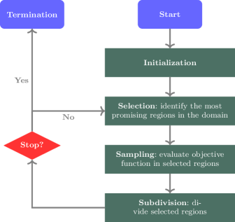
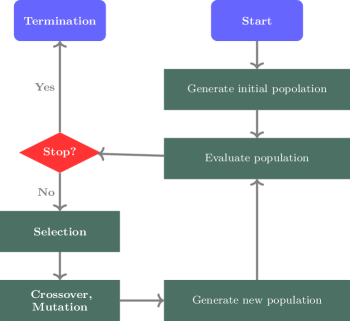
Figure 2: The basic structures of DIRECT-type (left side) and population-based (right side) algorithms.

Table 3: List of the deterministic algorithms (their implementations) in chronological order starting from the oldest.

Algorithm	Reference	Year	Impact	Class	Acronym	Implementation	Version
The original DIRECT	Jones1993	$1993$	$2,366$	DIRECT-type	DIRECT	DIRECTGO DIRECTGO2022	$1.1.0$
Multilevel coordinate search	Huyer1999	$1999$	$658$	MCS	MCS*	MCS* Arnold1999	$2.0$
Revised version of the DIRECT	Jones2001	$2001$	$401$	DIRECT-type	DIRECT-rev*	DIRECTGO DIRECTGO2022	$1.1.0$
Locally-biased form of the DIRECT	Gablonsky2001	$2001$	$365$	DIRECT-type	DIRECT-l	DIRECTGO DIRECTGO2022	$1.1.0$
Aggressive version of the DIRECT	Baker2000	$2001$	$73$	DIRECT-type	Ag. DIRECT	DIRECTGO DIRECTGO2022	$1.1.0$
Adaptive setting of the DIRECT parameters	Finkel2004aa	$2004$	$20$	DIRECT-type	DIRECT-restart	DIRECTGO DIRECTGO2022	$1.1.0$
Clustering technique-based hybridized DIRECT	Holmstrom2004	$2004$	$34$	DIRECT-type	glcCluster*	TOMLAB Holmstrom2010	$8.7$
Implementation of original DIRECT algorithm	Holmstrom2004	$2004$	$34$	DIRECT-type	glbSolve	TOMLAB Holmstrom2010	$8.7$
Multi-start scatter search algorithm	Holmstrom2004	$2004$	$34$	MS	OQNLP*	TOMLAB Holmstrom2010	$8.7$
Multi-start scatter search algorithm	Holmstrom2004	$2004$	$34$	MS	MSNLP*	TOMLAB Holmstrom2010	$8.7$
Hybridized branch-and-bound algorithm	Holmstrom2004	$2004$	$34$	BB	LGO*	TOMLAB Holmstrom2010	$8.7$
Additive scaling in DIRECT algorithm	Finkel2006	$2006$	$64$	DIRECT-type	DIRECT-m	DIRECTGO DIRECTGO2022	$1.1.0$
Adaptive diagonal curves	Sergeyev2006	$2006$	$118$	DIRECT-type	ADC	DIRECTGO DIRECTGO2022	$1.1.0$
Aggressively hybridized version of the DIRECT	Liuzzi2010	$2010$	$64$	DIRECT-type	DIRMIN*	DIRECTGO DIRECTGO2022	$1.1.0$
Linear scaling and the DIRECT algorithm	Liu2013	$2013$	$17$	DIRECT-type	DIRECT-a	DIRECTGO DIRECTGO2022	$1.1.0$
Simplicial partitioning technique based DIRECT	Paulavicius2013:jogo	$2013$	$58$	DIRECT-type	DISIMPL-C	DIRECTGO DIRECTGO2022	$1.1.0$
Simplicial partitioning technique based DIRECT	Paulavicius2013:jogo	$2013$	$58$	DIRECT-type	DISIMPL-V	DIRECTGO DIRECTGO2022	$1.1.0$
Multilevel DIRECT algorithm	Liu2015	$2015$	$30$	DIRECT-type	MrDIRECT${}_{\text{075}}$	DIRECTGO DIRECTGO2022	$1.1.0$
DIRECT using bisection of hyper-rectangles	Paulavicius2016:jogo	$2016$	$20$	DIRECT-type	BIRECT	DIRECTGO DIRECTGO2022	$1.1.0$
Pareto-Lipschitzian optimization	Mockus2017	$2017$	$16$	DIRECT-type	PLOR	DIRECTGO DIRECTGO2022	$1.1.0$
Pareto selection based DIRECT	Stripinis2018a	$2018$	$16$	DIRECT-type	DIRECT-G	DIRECTGO DIRECTGO2022	$1.1.0$
Two-step (Global-Local), selection based DIRECT	Stripinis2018a	$2018$	$16$	DIRECT-type	DIRECT-GL	DIRECTGO DIRECTGO2022	$1.1.0$
Globally-biased hybridized version of the BIRECT	Paulavicius2019:eswa	$2019$	$30$	DIRECT-type	BIRMIN*	DIRECTGO DIRECTGO2022	$1.1.0$
Globally-biased version of the BIRECT	Paulavicius2019:eswa	$2019$	$30$	DIRECT-type	Gb-BIRECT	DIRECTGO DIRECTGO2022	$1.1.0$
Improved aggressive version of the DIRECT-rev*	Stripinis2021b	$2022$	$0$	DIRECT-type	1-DTC-IA	DIRECTGO DIRECTGO2022	$1.1.0$
Improved aggressive version of the BIRECT	Stripinis2021b	$2022$	$0$	DIRECT-type	1-DBDV-IA	DIRECTGO DIRECTGO2022	$1.1.0$
Improved original selection based DIRECT-rev*	Stripinis2021b	$2022$	$0$	DIRECT-type	1-DTC-IO	DIRECTGO DIRECTGO2022	$1.1.0$
Improved original selection based BIRECT	Stripinis2021b	$2022$	$0$	DIRECT-type	1-DBDV-IO	DIRECTGO DIRECTGO2022	$1.1.0$
Two-step (Global-Local), selection based DIRECT-rev*	Stripinis2021b	$2022$	$0$	DIRECT-type	1-DTC-GL	DIRECTGO DIRECTGO2022	$1.1.0$
Two-step (Global-Local), selection based BIRECT	Stripinis2021b	$2022$	$0$	DIRECT-type	1-DBDV-GL	DIRECTGO DIRECTGO2022	$1.1.0$
* – Algorithm is hybridized with a local search procedures.

2.1.3 Multilevel coordinate search (MCS) algorithms

Similar to DIRECT, MCS partitions the search space into smaller hyper-rectangles. Each contains a distinguished point, the so-called base point, in which the objective function value is evaluated. The hyper-rectangular partitioning procedure is not uniform, and regions are preferred where better function values are expected to be found. Same as in DIRECT, MCS solver typically combine global search (a subdivision of the largest hyper-rectangles) and local search (a subdivision of the hyper-rectangles with good function values). The MCS* algorithm carries the multilevel technique for balancing global and local search in each iteration. MCS* was the only one included in our study of this class (see Table 3).

2.1.4 Multi-start (MS) search algorithms

The multi-start technique Hey1979 is a well-known stochastic approach that attempts to run local search procedures from a set of random starting points. When the initial points are chosen in a non-random way, the algorithm acquires the property of determinism. From this class, we consider two solvers (OQNLP* and MSNLP*), designed to find global optima of smooth constrained and mixed-integer nonlinear problems.

To summarize, the main advantages of deterministic techniques are the guarantee of the same result (output) and a typically low number of algorithmic input parameters Jones2021 . The main disadvantage is the limited efficiently on higher-dimensional global optimization problems Jones2021 ; Rios2013 .

2.2 Stochastic global search algorithms

Due to the non-deterministic nature, the guarantee of the optimal solution in stochastic algorithms is provided only in a probabilistic sense. The convergence of most stochastic techniques is based on the classical probability theory, “zero-one law.” In the following subsections, we will review several well-known classes of stochastic algorithms from which algorithms were chosen for this study (see Table 4). The structure of Table 3 is the same as for Table 4. The only difference is that in the last column, we specify the nature of the algorithm.

2.2.1 Pure Random Search (PRS)

The most straightforward stochastic global optimization is pure random search (PRS), implemented as Monte-Carlo algorithm (see Table 4). A set of uniformly distributed random points is generated in every iteration, and the objective function values at these points are recorded. The generation of the new points is constructed independently of previous sampled points, i.e., PRS does not use information from previous iterations. For this reason, the performance of the PRS technique is considered unrelated to the structure of the objective function.

2.2.2 Markovian Global Search (MGS)

MGS algorithms are yet simple but cleverer than PRS. The distribution of the points in MGS depends on the previously sampled point and the current best-recorded function value. The main criticism of MGS class algorithms is that they are often too myopic and do not make efficient use of information about the objective function achieved earlier. The most popular in this class is the well-known simulated annealing algorithm, which also has the highest impact score among all the considered algorithms (see Table 4).

Table 4: List of the stochastic algorithms (their implementations) in chronological order starting from the oldest.

Algorithm	Reference	Year	Impact	Class	Acronym	Implementation	Version	Based on
Monte-Carlo algorithm	Metropolis1949	$1955$	$8,117$	PRS	MC	MIC Tche2022	$1.0$	Random
Genetic algorithm	Holland1975	$1975$	$38,629$	PBS	ga	MATLAB MATLAB2022	$9.12.0$	Evolutionary
Simulated annealing	Kirkpatrick1983a	$1983$	$53,379$	MGS	simulannealbnd	MATLAB MATLAB2022	$9.12.0$	Nature
Adaptive Monte-Carlo algorithm	Patel1989	$1989$	$112$	PAS	AMC	MIC Tche2022	$1.0$	Random
Ant colony optimization	Dorigo1992O	$1992$	$16,032$	PBS	ACO	YPEA Kalami2020	$1.1.0.4$	Swarm
Cultural algorithm	Reynolds2008	$1994$	$1,258$	PBS	CA	YPEA Kalami2020	$1.1.0.4$	Evolutionary
Particle swarm optimization	Eberhart1995	$1995$	$17,922$	PBS	PSO	YPEA Kalami2020	$1.1.0.4$	Swarm
Differential evolution	Storn1997	$1997$	$29,527$	PBS	DE	YPEA Kalami2020	$1.1.0.4$	Population
Surrogate optimization algorithm	Gutmann2001	$2001$	$863$	MBO	surrogateopt	MATLAB MATLAB2022	$9.12.0$	Model-based
Harmony search	Geem2001	$2001$	$6,457$	PBS	HS	YPEA Kalami2020	$1.1.0.4$	Nature
Shuffled Frog Leaping Algorithm	Muzaffar2003	$2003$	$1,850$	PBS	SFLA	SFLA Yarpiz2022	$1.0.0.0$	Bio
Multi-start global random search	Holmstrom2004	$2004$	$34$	RMS	MULTIMIN*	TOMLAB Holmstrom2010	$8.7$	Random
Artificial bee colony	Karaboga2005ANIB	$2005$	$7,669$	PBS	ABC	YPEA Kalami2020	$1.1.0.4$	Swarm
Bees algorithm	Pham2006	$2006$	$1,535$	PBS	BE	YPEA Kalami2020	$1.1.0.4$	Swarm
Invasive Weed Optimization	Mehrabian2006	$2006$	$1,441$	PBS	IWO	YPEA Kalami2020	$1.1.0.4$	Swarm
Imperialist Competitive Algorithm	Gargari2007	$2007$	$2,912$	PBS	ICA	YPEA Kalami2020	$1.1.0.4$	Evolutionary
Multi-start global random search	Ugray2007	$2007$	$697$	RMS	MultiStart*	MATLAB MATLAB2022	$9.12.0$	Random
Multi-start global random search	Ugray2007	$2007$	$697$	RMS	GlobalSearch*	MATLAB MATLAB2022	$9.12.0$	Random
Stochastic Radial Basis Function	Regis2007	$2007$	$422$	MBO	StochasticRBF	StochasticRBF Julie2006	$1.0.0.0$	Model-based
Biogeography-based Optimization	Dan2008	$2008$	$3,659$	PBS	BBO	YPEA Kalami2020	$1.1.0.4$	Nature
Firefly algorithm	Yang2009as	$2009$	$4,306$	PBS	FA	YPEA Kalami2020	$1.1.0.4$	Swarm
Cuckoo search	Yang2009a	$2009$	$6,772$	PBS	CS	CS Yang2022a	$2.0.0$	Swarm
Bat-Inspired Algorithm	Yang2010as	$2010$	$5,179$	PBS	BAT	BAT Yang2022b	$2.0.0$	Swarm
Covariance matrix adaptation strategy	Iruthayarajan2010	$2010$	$72$	PBS	CMA-ES	YPEA Kalami2020	$2.0.0$	Evolutionary
Teaching-Learning-based Optimization	Rao2011	$2011$	$3,307$	PBS	TLBO	YPEA Kalami2020	$1.1.0.4$	Population
Improved State Transition Algorithm	Saravanakumar2015	$2015$	$4$	PBS	STA	STA sta2022	$1.0$	Population
Bayesian Adaptive Direct Search	Acerbi2017	$2017$	$152$	MBO	BADS	BADS Acerbi2022	$1.0.8$	Model-based
Chaotic neural network algorithm	Sadollah2018	$2018$	$125$	PBS	CNNA	CNNA Zhang2022	$1.0.0$	Bio
Neural Network Algorithm	Sadollah2018dynamic	$2018$	$130$	PBS	NNA	NNA Sadollah2018dynamic	$1.0.0$	Bio
Bald Eagle search optimization	Alsattar2020	$2020$	$100$	PBS	BESO	BESO Hassan2022	$1.0.0$	Nature
Fuzzy self-tuning differential evolution	Tsafarakis2020	$2020$	$19$	PBS	fstde	fstde Tsafarakis2020	$2.0.0$	Population
African Vulture Optimization algorithm	Abdollahzadeh2021	$2021$	$101$	PBS	AVOA	AVOA Abdollahzadeh2021	$1.0.2$	Nature
Atomic Orbital Search	Azizi2021	$2021$	$33$	PBS	AOS	AOS Azizi2022	$1.0.0$	Quantum
Sand Cat swarm optimization	Seyyedabbasi2022	$2022$	$0$	PBS	SCSO	SCSO amir2022	$1.0.0$	Nature
* – Algorithm is hybridized with local search procedures.

2.2.3 Pure Adaptive Search (PAS)

The PAS approach starts by generating a point uniformly distributed within the optimization domain, where the objective function value is recorded. The next point is generated from a uniform distribution over the region constructed by the intersection of the whole optimization region with the open level set of points with objective function values less than the best-recorded value. The approach proceeds iteratively in this manner until some stopping criterion is satisfied. This way, PAS performs samples in that part of the optimization domain that gives a strictly improving objective function value at each iteration. PAS technique has been implemented in the adaptive Monte-Carlo algorithm (see Table 4).

2.2.4 Random Multi-Start (RMS)

The multi-start calls a local search procedure with different initial values and returns the solutions and the optimal point from each started point. Random multi-start (RMS) is a well-known and well known global optimization algorithm in practice. Local search procedures are performed from several random points in the optimization domain. The point can be generated using PRS (as in the MULTIMIN*, MultiStart*, and GlobalSearch* algorithms) or PAS techniques.

2.2.5 Population-Based Search (PBS)

The population (set of points) evolves in PBS algorithms rather than single points. There are many publications on PBS, the majority of which deal with meta-heuristics rather than theory and generic methodology. The term “meta-heuristic” has been known for almost four decades GLOVER1986533 . Meta-heuristics are high-level random search techniques designed to intelligently locate optimal or at least near-optimal solutions for complex optimization problems Blum2003 . As many as $25$ meta-heuristic algorithms were used in this study (see Table 4).

In Gharehchopogh2019a ; Gharehchopogh2020 , the authors concluded that the design and development of meta-heuristic algorithms had been studied more than other optimization techniques due to four main factors: i) meta-heuristic algorithms are inspired by relatively simple concepts from nature that make them easy to implement; ii) these algorithms have many input parameters to control the performance efficiency without altering the algorithm’s structure, making them flexible solving various optimization problems; iii) most meta-heuristic algorithms are derivation-free; iv) meta-heuristic algorithms often escape from local optimum better than other algorithms.

The majority of meta-heuristic algorithms are based on biological evolution principles. In particular, they are based on simulations of various biological metaphors which differ in the nature of the representation schemes (structure, components, etc.). The two most common paradigms are evolutionary and swarm systems BLUM20114135 ; BOUSSAID201382 ; Zavala2014 .

Evolutionary algorithms. In the last decades, there has been a significant interest in evolutionary algorithms, which are based on the principles of natural evolution JangaReddy2020 . Evolutionary Algorithms simulate the biological progression of evolution at the cellular level using selection, crossover, mutation, and reproduction operators to generate increasingly better candidate solutions (chromosomes). The algorithms consist of a population of individuals, each representing a search point in the optimization domain. They are exposed to a collective learning process that proceeds from one generation to another. The initial population is randomly generated and then subjected to selection, crossover, and mutation procedures over several generations to force the newly produced generations to move into more favorable regions of the optimization domain. The progress in the search is achieved by evaluating the fitness (objective function) of all individuals in the population, selecting individuals with a better fitness value, and combining them to create new individuals with a higher probability of improving the previous fitness. In the long sequence of the generations, the algorithms converge, and the best individual represents the solution. Many different evolutionary approaches have been developed, but the basic algorithmic structure is very much the same for all the algorithms, see right side of Fig. 2.

The most popular evolutionary approach is the genetic algorithm (GA) Holland1975 (see Table 4). The GA is a population-based probabilistic search algorithm based on natural selection and genetics mechanics. A genetic algorithm begins its search with a set of individuals, called population, randomly generated to cover the entire search space uniformly. Individuals are associated with identity genes that define a fitness measure. Then, evaluation of the fitness, selection of parents, applying genetic operations, crossover operator for creating offspring, and mutation operation for perturbing the individuals to produce a new population is performed. The selection operator utilizes the “survival of the fittest” concept from Darwinian evolution theory and uses probabilistic rules to select the fittest candidate solutions (best in terms of the objective function) in the current population. The iterative process is repeated until one of the stopping conditions is satisfied.

Swarm intelligence. Swarm intelligence (or bio-inspired computation) is an integral part of the field of artificial intelligence. Mainly motivated by biological systems, swarm intelligence adopts the collective behavior of an organized group of animals as they seek to survive. The main algorithms that fall under swarm intelligence approaches include ant colony optimization (ACO) Dorigo1992O , particle swarm optimization (PSO) Eberhart1995 , artificial bee colony (ABC) Karaboga2005ANIB , bees algorithm (BE) Pham2006 , invasive weed optimization (IWO) Mehrabian2006 , firefly algorithms (FA) Yang2009as , cuckoo search (CS) Yang2009a , bat-inspired algorithm (BAT) Yang2010as . Similar to evolutionary algorithms, swarm intelligence models are population-based iterative solvers. The search begins with a randomly initialized population of individuals. These individuals are then iteratively manipulated and evolved by mimicking the behavior of insects or animals to find the optimum solution.

2.2.6 Model-based optimization (MBO)

Model-based optimization algorithms generate a population of new points by sampling from a model (or a distribution). The model (or a distribution) guides structural properties of the underlying real objective function $f$. Model-based optimization algorithms are based on the concept that the search is directed into regions with improved solutions by adopting the model (or the distribution). One of the essential ideas in model-based optimization is to substitute the expensive evaluations of the real objective function $f$ with evaluations of a cheap, grained model $\hat{f}$.

Bayesian optimization Jones1998 is one of the most popular model-based state-of-the-art machine learning frameworks for optimizing expensive black-box functions. The Bayesian optimization constructs a Gaussian process to approximate the objective function. A built model is a relatively low-cost surrogate to help guide the search toward promising/unknown regions. Three MBO technique-based algorithms are considered in this survey: the Bayesian adaptive direct search Acerbi2017 , surrogate optimization algorithm Gutmann2001 , and stochastic radial basis Function Regis2007 (see Table 4).

To sum up, the main advantages of stochastic techniques are robust performance on different optimization problems, including high-dimensional ones, and relative simplicity of implementation. At the same time, as main disadvantages are dependency on numerous input parameters zilinskas_zhigljavsky_2016 and the possibility of very slow convergence.

2.3 Additionally tested solvers

We have additionally investigated more solvers in this study. Here we briefly mention them and why they were not included in the final comparison:

1. TOMLAB/EGO – Implementation of efficient global optimization algorithm for expensive “black-box” functions Jones1998 .

2. TOMLAB/rbfSolve – Implementation of the radial basis function-based approach Bjorkman2000 that can handle expensive box-constrained “black-box” global optimization problems.

3. MATLAB/bayesopt – Implement the Bayesian optimization Bjorkman2000 that can handle expensive box-constrained “black-box” global optimization problems.

4. 1-DTDV-IA Implementation of the improved aggressive version of the ADC algorithm Stripinis2021b .

5. 1-DTDV-GL Implementation of the two-step-based (Global-Local) Pareto selection-based ADC algorithm Stripinis2021b .

The EGO, rbfSolve, and bayesopt algorithms are designed specifically for expensive objective functions, but the amount of computation involved in algorithmic steps has made these algorithms extremely slow. Similarly, the ADC algorithm’s partitioning scheme is considered slow, especially in high dimensions. The above-mentioned algorithms were not considered in further comparison studies for these reasons.

3 Experimental design

3.1 Test problems

This study uses two problem suites: DIRECTGOLib v1.2 DIRECTGOLib2022 and GKLS test problem generator Gaviano2003 . Problem attributes of uni-modality or multi-modality, low or high dimensional, and convex or non-convex geometries are covered.

3.1.1 GKLS test problems

The GKLS software Gaviano2003 generates non-differentiable, continuously differentiable, and twice continuously differentiable classes of test functions for multi-modal, multi-dimensional box-constrained global optimization. For each generated problem, all local and global minima are known. The test problems are constructed by defining a convex quadratic function (paraboloid) systematically distorted by polynomials to produce local minima. Each class of problems consists of 100 test functions. The complexity of the class is determined using the following parameters: problem dimension $(n)$, number of local minima $(h)$, the value of the global minimum $(f^{*})$, radius $(r)$ of the attraction region of the global minimizer and the distance $(d)$ from the global minimizer to the vertex of the quadratic function. The complete repeatability of experiments is an essential feature of the generator. If the same five parameters are provided to GKLS, the identical class of functions will be produced each time the generator is executed.

We use standard eight different complexity classes (see Table 5), which are the most widely and commonly used in other numerical studies Sergeyev2006 ; Paulavicius2014:jogo ; Paulavicius2019:eswa ; Stripinis2021b . The dimension ($n$) of generated test classes and other parameters are the same as in other mentioned studies. For each dimension $n$, two test classes were considered: the “simple” class and the “hard” one. For third and fourth dimensional classes, the difficulty is increased by enlarging the distance $d$ from the global optimum point $(\mathbf{x}^{*})$ to the paraboloid vertex. For second and fifth dimensional classes, this is achieved by decreasing the radius $r$.

Table 5: GKLS test classes used in numerical experiments.

Class	$\#$	Difficulty	$n$	$f^{*}$	$d$	$r$	$h$
$1$	$100$	simple	$2$	$-1$	$0.90$	$0.20$	$10$
$2$	$100$	hard	$2$	$-1$	$0.90$	$0.10$	$10$
$3$	$100$	simple	$3$	$-1$	$0.66$	$0.20$	$10$
$4$	$100$	hard	$3$	$-1$	$0.90$	$0.20$	$10$
$5$	$100$	simple	$4$	$-1$	$0.66$	$0.20$	$10$
$6$	$100$	hard	$4$	$-1$	$0.90$	$0.20$	$10$
$7$	$100$	simple	$5$	$-1$	$0.66$	$0.30$	$10$
$8$	$100$	hard	$5$	$-1$	$0.66$	$0.20$	$10$

3.1.2 DIRECTGOLib v1.2 test set

The second set of test problems chosen for the experiments comprises more traditional cases collected from the literature. Test problems from the most recent and significantly expanded ($69$ new test problems, including 18 published this year Layeb2022 ) DIRECTGOLib v1.2 DIRECTGOLib2022 library are used to evaluate considered algorithms.

Overview of all employed box-constrained optimization test problems from DIRECTGOLib v1.2 and their properties are given in Appendix 7 Tables 13 and 12. Here, the main features are reported: problem number (#), name of the problem, source, dimensionality ($n$), optimization domain ($D$), problem type, and the known minimum ($f^{*}$). Moreover, the original domains $D$ for some problems are perturbed ($\tilde{D}$) that the solutions are not located in their midpoints or other points favorable for any deterministic algorithms. Finally, newly added test problems are marked with the symbol $\beta$.

Some of these test problems have several variants, e.g., Ackley, Hartman, Shekel, and some of them, like Alpine, Csendes, Griewank, etc., can be tested for varying dimensionality. The $67$ test problems listed in Table 13 have fixed dimensions, while Table 12 presents $55$ test benchmarks that can be used by specifying any dimension size ($n$). For these test problems instances with $n=2,5,10,20,50,$ and $100$ variables were considered, leading in total to $397$ test problems (see summary in Table 6).

Various subsets (e.g., non-convex, multi-modal, etc.) of the whole set were used to deepen the investigation. The low-dimensional ($n\leq 10$) test set is designed to evaluate the performance of solvers on relatively small dimensional problems. The high-dimensional ($n\geq 11$) test set is used to test the efficiency of solvers on higher dimensions.

Table 6: Characteristics of DIRECTGOLib v1.2 test problems.

Dimension / type	convex	non-convex	uni-modal	multi-modal
$n\leq 10$	$55$	$176$	$41$	$190$
$n\geq 11$	$42$	$124$	$36$	$130$
Total	$97$	$300$	$77$	$320$

3.2 Experimental setup and basis of solver comparisons

All computations were performed on Intel R Core${}^{\textit{TM}}$ i5-10400 @ 2.90GHz Processor running MATLAB R2022a. The solutions returned by the solvers against the globally optimal solution for each problem were compared. A solver was considered to have successfully solved the test problem during a run if it returned a solution with an objective function value within $1\%$. For all analytical test cases with a priori known global optima $f^{*}$, the used stopping criterion is based on the percent error $(pe)$:

$$\ pe=100\%\times\begin{cases}\frac{f({\mathbf{x}})-f^{*}}{\mid f^{*}\mid},&f^{*}\neq 0,\\ f({\mathbf{x}}),&f^{*}=0,\end{cases}$$ (2)

where $f^{*}$ is the known global optimum. The algorithms were stopped when the percent error became smaller than the prescribed value $\varepsilon_{\rm pe}=1$ or when the number of function evaluations exceeded the prescribed limit ($M_{\rm max}$). We note that when the optimal value is large, the algorithm will terminate when the distance to the optimum is relatively large. However, there were only a few such tasks in the test set.

We used two different values of $M_{\rm max}$. First, like in Rios2013 , we use $2,500$ to evaluate which algorithms perform best for expensive objective problems. Additionally, $M_{\rm max}=500,000$ is used to evaluate the performance when the objective function evaluations are cheap. As all algorithms were implemented in the same environment (MATLAB), additionally we included the execution time in the comparison. A limit ($T_{\rm max}$) of $3,600$ CPU seconds was imposed on each run.

3.3 Algorithmic settings

The number of chosen algorithms is extensive, they are very different, and various algorithmic control structures determine their effectiveness. Algorithms also have different input parameters that can have a significant impact their performance. For example, DIRECT-type algorithms have a much smaller number of input parameters than meta-heuristic solvers, some of whom have none at all (e.g., Ag. DIRECT, DIRECT-G and DIRECT-GL from DIRECTGO toolbox Stripinis2021c ; DIRECTGO2022 ). The input parameters should be set in such a way as to ensure the best performance. Unfortunately, different input parameter values can drastically impact the algorithm’s performance. Thus, following the same idea used in the Rios2013 ; Stripinis2021c study, comparisons were carried out using the default parameter values for each algorithm.

Among the $64$ algorithms involved in the study, $11$ are hybridized with local search procedures. All of them are distinguished by adding the * symbol at the end of the title. Most of these algorithms (DIRECT-rev*, DIRMIN*, BIRMIN*, MultiStart*, and GlobalSearch*) are hybridized using the interior-point Byrd2000 algorithm, implemented in MATLAB nonlinear programming solver – fmincon. TOMLAB’s global optimization algorithms hybridize with SNPOT or NPSOL Holmstrom2010 local minimizers. No derivative information was provided for them. Thus, if needed, the local solvers could only use the function values to approximate gradients, e.g., by a finite difference technique. However, the use of finite differences has been broadly dismissed in the derivative-free literature as expensive in terms of function evaluations Shi2021 .

3.4 Benchmarking derivative-free optimization solvers

To analyze and compare the algorithms’ performance, we applied the data profiles More2009 to the convergence test (2). The data profile is a popular and widely used tool for bench-marking and evaluating the performance of several algorithms (solvers) when run on a large problem set. Benchmark results are generated by running a certain algorithm $v$ (from a set of algorithms $\mathcal{V}$ under consideration) for each problem $u$ from a benchmark set $\mathcal{U}$ and recording the performance measure of interest. The performance measure could be, for example, the number of function evaluations, the computation time, the number of iterations, or the memory used. We used a number of function evaluations and the execution (computation) time criteria.

The data profiles provide the percentage of problems that can be solved with a given budget of the desired performance measure. The data profile is defined

$$\lambda_{v}(\alpha)=\frac{1}{card(\mathcal{U})}\textrm{size}\left\{u\in\mathcal{U}:t_{u,v}\leq\alpha\right\},$$ (3)

where $t_{u,v}>0$ is the number of performance measure required to solve problem $u$ by the algorithm $v$, and $card(\mathcal{U})$ is the cardinality of $\mathcal{U}$. In our case, the $\lambda_{v}(\alpha)$ shows the percentage of problems that can be solved within $\alpha$ function evaluations, or seconds.

4 Numerical results

4.1 Computational results solving GKLS test problems

Numerical results on eight GKLS test classes from Table 5 are reported in Tables 7 and 8 for “simple” and “hard” classes of GKLS test problems using two different $M_{\rm max}$ values. The best results are given in bold. In both tables, the algorithms are ranked based on the average success rate (S.R.) reported in the sixth and eleventh columns.

Table 7: The average number ($f_{\rm avg.}$) and standard deviation ($f_{\rm s.d.}$) of function evaluations, the average value ($t_{\rm avg.}$) and standard deviation ($t_{\rm s.d.}$) of execution time, and the success rate (S. R.) for “simple” GKLS test problems using $M_{\rm max}=2,500$ and $M_{\rm max}=500,000$.

Evaluation budget	$M_{\rm max}=2,500$					$M_{\rm max}=500,000$
Criteria	$f_{\rm avg.}$	$f_{\rm s.d.}$	$t_{\rm avg.}$	$t_{\rm s.d.}$	S. R.	$f_{\rm avg.}$	$f_{\rm s.d.}$	$t_{\rm avg.}$	$t_{\rm s.d.}$	S. R.
BIRMIN*	$\mathbf{1,163}$	$-$	$0.21$	$-$	$\mathbf{0.73}$	$\mathbf{1,991}$	$-$	$0.40$	$-$	$\mathbf{1.00}$
Gb-BIRECT	$1,235$	$-$	$0.20$	$-$	$0.69$	$2,243$	$-$	$0.44$	$-$	$\mathbf{1.00}$
MSNLP*	$1,663$	$-$	$0.30$	$-$	$0.69$	$7,361$	$-$	$1.84$	$-$	$0.99$
DIRECT-a	$1,219$	$-$	$0.11$	$-$	$0.67$	$4,154$	$-$	$0.34$	$-$	$\mathbf{1.00}$
DIRECT-m	$1,233$	$-$	$0.12$	$-$	$0.67$	$5,080$	$-$	$0.42$	$-$	$\mathbf{1.00}$
MrDIRECT${}_{\text{075}}$	$1,288$	$-$	$0.24$	$-$	$0.67$	$7,785$	$-$	$1.42$	$-$	$\mathbf{1.00}$
DIRECT-G	$1,305$	$-$	$0.07$	$-$	$0.67$	$5,587$	$-$	$0.27$	$-$	$\mathbf{1.00}$
DIRECT	$1,231$	$-$	$0.18$	$-$	$0.66$	$4,284$	$-$	$0.37$	$-$	$\mathbf{1.00}$
glbSolve	$1,233$	$-$	$0.13$	$-$	$0.66$	$4,279$	$-$	$0.59$	$-$	$\mathbf{1.00}$
DIRECT-rev*	$1,288$	$-$	$0.19$	$-$	$0.66$	$3,839$	$-$	$0.54$	$-$	$\mathbf{1.00}$
BIRECT	$1,312$	$-$	$0.20$	$-$	$0.64$	$4,139$	$-$	$0.59$	$-$	$\mathbf{1.00}$
1-DBDV-IO	$1,312$	$-$	$0.21$	$-$	$0.64$	$4,139$	$-$	$0.62$	$-$	$\mathbf{1.00}$
1-DBDV-GL	$1,459$	$-$	$0.56$	$-$	$0.64$	$6,018$	$-$	$0.79$	$-$	$\mathbf{1.00}$
1-DTC-IO	$1,314$	$-$	$0.19$	$-$	$0.63$	$4,145$	$-$	$0.72$	$-$	$\mathbf{1.00}$
DIRECT-restart	$1,197$	$-$	$4.65$	$-$	$0.70$	$46,770$	$-$	$163.30$	$-$	$0.92$
DIRECT-GL	$1,465$	$-$	$0.09$	$-$	$0.62$	$7,010$	$-$	$0.36$	$-$	$\mathbf{1.00}$
1-DTC-GL	$1,391$	$-$	$0.08$	$-$	$0.61$	$8,879$	$-$	$0.32$	$-$	$\mathbf{1.00}$
1-DBDV-IA	$1,537$	$-$	$1.65$	$-$	$0.58$	$10,543$	$-$	$1.41$	$-$	$\mathbf{1.00}$
glcCluster*	$1,620$	$-$	$0.76$	$-$	$0.57$	$4,704$	$-$	$2.14$	$-$	$\mathbf{1.00}$
OQNLP*	$1,532$	$-$	$0.44$	$-$	$0.57$	$32,194$	$-$	$10.88$	$-$	$0.99$
MCS*	$1,601$	$-$	$1.15$	$-$	$0.55$	$7,879$	$-$	$4.73$	$-$	$\mathbf{1.00}$
ADC	$1,565$	$-$	$5.19$	$-$	$0.54$	$4,429$	$-$	$12.16$	$-$	$\mathbf{1.00}$
1-DTC-IA	$1,524$	$-$	$0.06$	$-$	$0.54$	$16,281$	$-$	$1.27$	$-$	$\mathbf{1.00}$
DIRECT-l	$1,440$	$-$	$1.67$	$-$	$0.55$	$27,988$	$-$	$11.44$	$-$	$0.98$
DISIMPL-V	$1,528$	$-$	$3.69$	$-$	$0.50$	$18,793$	$-$	$103.62$	$-$	$0.98$
DISIMPL-C	$1,664$	$-$	$5.31$	$-$	$0.45$	$49,439$	$-$	$488.99$	$-$	$0.97$
Ag. DIRECT	$1,809$	$-$	$0.09$	$-$	$0.43$	$34,903$	$-$	$1.37$	$-$	$0.98$
DIRMIN*	$1,901$	$-$	$0.32$	$-$	$0.41$	$23,477$	$-$	$3.72$	$-$	$\mathbf{1.00}$
PLOR	$1,577$	$-$	$4.16$	$-$	$0.47$	$88,448$	$-$	$293.94$	$-$	$0.88$
simulannealbnd	$1,972$	$432$	$1.24$	$4.41$	$0.36$	$21,497$	$16,336$	$21.14$	$82.60$	$0.99$
MultiStart*	$2,000$	$410$	$3.49$	$4.18$	$0.36$	$21,515$	$16,827$	$16.32$	$26.75$	$0.99$
StochasticRBF	$2,010$	$318$	$2.18$	$7.54$	$0.31$	$34,851$	$21,410$	$147.17$	$259.58$	$0.99$
SCSO	$1,825$	$306$	$1.33$	$5.50$	$0.41$	$80,896$	$53,683$	$10.02$	$13.71$	$0.86$
surrogateopt	$1,486$	$251$	$72.91$	$55.00$	$0.56$	$159,431$	$64,750$	$1,156.32$	$1,620.79$	$0.68$
BE	$1,978$	$278$	$0.51$	$0.18$	$0.42$	$123,802$	$105,942$	$16.33$	$28.34$	$0.76$
STA	$2,409$	$78$	$1.34$	$5.93$	$0.31$	$89,792$	$71,245$	$10.02$	$13.71$	$0.84$
AVOA	$1,984$	$340$	$0.03$	$0.01$	$0.34$	$125,968$	$70,637$	$1.73$	$2.72$	$0.80$
LGO*	$2,267$	$-$	$1.25$	$-$	$0.14$	$135,346$	$-$	$15.87$	$-$	$0.98$
MULTIMIN*	$2,470$	$17$	$0.33$	$0.17$	$0.13$	$25,702$	$4,193$	$3.26$	$7.51$	$0.98$
AOS	$2,026$	$373$	$0.13$	$0.05$	$0.32$	$162,610$	$69,751$	$10.02$	$13.71$	$0.76$
HS	$2,112$	$331$	$0.31$	$0.05$	$0.32$	$171,004$	$79,453$	$22.66$	$29.10$	$0.72$
AMC	$2,015$	$147$	$0.11$	$0.04$	$0.45$	$205,638$	$100,081$	$10.30$	$12.26$	$0.59$
GlobalSearch*	$2,500$	$0$	$0.52$	$0.00$	$0.00$	$29,892$	$19,291$	$6.48$	$10.03$	$0.99$
NNA	$2,292$	$150$	$0.08$	$0.01$	$0.22$	$140,758$	$71,521$	$1.29$	$1.79$	$0.75$
CNNA	$2,313$	$151$	$0.07$	$0.01$	$0.15$	$116,336$	$62,272$	$2.56$	$4.30$	$0.81$
PSO	$1,899$	$364$	$0.26$	$0.11$	$0.46$	$259,194$	$135,680$	$35.71$	$34.56$	$0.48$
ICA	$1,926$	$395$	$0.63$	$0.33$	$0.39$	$257,268$	$171,481$	$77.32$	$76.06$	$0.49$
ABC	$2,382$	$123$	$0.34$	$0.05$	$0.12$	$178,138$	$58,343$	$24.97$	$30.87$	$0.73$
CS	$2,373$	$127$	$0.03$	$0.01$	$0.15$	$154,038$	$139,577$	$1.84$	$2.72$	$0.69$
BESO	$2,230$	$192$	$0.07$	$0.02$	$0.24$	$254,856$	$112,329$	$7.62$	$7.41$	$0.49$
SFLA	$1,861$	$520$	$1.22$	$5.21$	$0.36$	$320,261$	$145,928$	$16.34$	$12.26$	$0.36$
TLBO	$2,215$	$260$	$0.32$	$0.09$	$0.25$	$287,069$	$126,127$	$39.51$	$33.79$	$0.44$
ga	$2,055$	$408$	$4.06$	$9.33$	$0.31$	$341,106$	$146,438$	$25.41$	$17.82$	$0.32$
BADS	$2,309$	$222$	$22.63$	$21.33$	$0.12$	$269,637$	$186,611$	$1,955.32$	$1,372.54$	$0.47$
fstde	$2,167$	$319$	$0.33$	$3.12$	$0.24$	$327,605$	$159,995$	$3.66$	$12.63$	$0.35$
BBO	$2,113$	$464$	$0.34$	$0.12$	$0.22$	$392,402$	$125,295$	$63.88$	$34.24$	$0.22$
IWO	$2,096$	$380$	$0.23$	$0.09$	$0.21$	$393,382$	$109,053$	$43.65$	$22.97$	$0.21$
FA	$2,075$	$510$	$0.37$	$0.15$	$0.20$	$398,582$	$123,555$	$64.66$	$33.29$	$0.20$
ACO	$2,267$	$285$	$0.32$	$0.08$	$0.14$	$405,410$	$113,734$	$65.94$	$33.39$	$0.19$
MC	$2,465$	$62$	$0.10$	$0.01$	$0.03$	$365,777$	$23,752$	$15.04$	$8.78$	$0.30$
DE	$2,171$	$415$	$0.50$	$0.18$	$0.15$	$422,807$	$98,451$	$98.60$	$43.70$	$0.15$
BAT	$2,304$	$267$	$0.04$	$0.01$	$0.09$	$452,293$	$66,491$	$7.77$	$2.82$	$0.09$
CMA-ES	$2,461$	$61$	$0.03$	$0.00$	$0.03$	$495,015$	$23,339$	$6.28$	$2.11$	$0.03$
CA	$2,466$	$36$	$0.32$	$0.03$	$0.02$	$487,905$	$12,731$	$62.01$	$10.49$	$0.02$

4.1.1 Comparison on “simple” GKLS problems with $M_{\rm max}=2,500$

The second, third, and sixth columns in Table 7 show the average number of function evaluations ($f_{\rm avg.}$), standard deviation ($f_{\rm s.d.}$), and success rate (S. R.) for all $400$ “simple” GKLS-type problems using $M_{\rm max}=2,500$. The hybridized BIRMIN* algorithm showed the best average number of function evaluations, solving $292$ problems within a budget of $2,500$ function evaluations. The best BIRMIN* algorithm is closely followed by the DIRECT-restart, which solved $280$, while Gb-BIRECT and MSNLP* solved $276$ test problems.

Table 8: The average number ($f_{\rm avg.}$) and standard deviation ($f_{\rm s.d.}$) of function evaluations, the average value ($t_{\rm avg.}$) and standard deviation ($t_{\rm s.d.}$) of execution time, and the success rate (S. R.) for “hard” GKLS test problems using $M_{\rm max}=2,500$ and $M_{\rm max}=500,000$.

Evaluation budget	$M_{\rm max}=2,500$					$M_{\rm max}=500,000$
Criteria	$f_{\rm avg.}$	$f_{\rm s.d.}$	$t_{\rm avg.}$	$t_{\rm s.d.}$	S. R.	$f_{\rm avg.}$	$f_{\rm s.d.}$	$t_{\rm avg.}$	$t_{\rm s.d.}$	S. R.
Gb-BIRECT	$\mathbf{1,594}$	$-$	$0.28$	$-$	$\mathbf{0.54}$	$7,482$	$-$	$1.91$	$-$	$\mathbf{1.00}$
BIRMIN*	$1,638$	$-$	$0.31$	$-$	$\mathbf{0.54}$	$\mathbf{7,384}$	$-$	$1.94$	$-$	$\mathbf{1.00}$
BIRECT	$1,795$	$-$	$0.28$	$-$	$0.46$	$18,735$	$-$	$4.22$	$-$	$\mathbf{1.00}$
1-DBDV-IO	$1,795$	$-$	$0.28$	$-$	$0.46$	$18,735$	$-$	$3.97$	$-$	$\mathbf{1.00}$
1-DTC-IO	$1,876$	$-$	$0.17$	$-$	$0.44$	$21,633$	$-$	$3.17$	$-$	$\mathbf{1.00}$
DIRECT-a	$1,838$	$-$	$0.18$	$-$	$0.44$	$24,121$	$-$	$2.51$	$-$	$0.99$
glbSolve	$1,847$	$-$	$0.21$	$-$	$0.44$	$25,604$	$-$	$10.05$	$-$	$0.99$
DIRECT	$1,847$	$-$	$0.28$	$-$	$0.44$	$31,770$	$-$	$73.64$	$-$	$0.99$
DIRECT-rev*	$1,907$	$-$	$0.30$	$-$	$0.42$	$31,176$	$-$	$5.50$	$-$	$0.99$
1-DBDV-GL	$1,880$	$-$	$1.09$	$-$	$0.42$	$52,264$	$-$	$3.18$	$-$	$0.98$
DIRECT-m	$1,892$	$-$	$0.20$	$-$	$0.40$	$32,943$	$-$	$3.62$	$-$	$0.99$
glcCluster*	$2,071$	$-$	$1.03$	$-$	$0.38$	$23,717$	$-$	$102.25$	$-$	$0.99$
ADC	$2,011$	$-$	$6.87$	$-$	$0.36$	$17,156$	$-$	$302.90$	$-$	$\mathbf{1.00}$
DIRECT-G	$2,007$	$-$	$0.13$	$-$	$0.32$	$50,997$	$-$	$3.14$	$-$	$0.98$
MCS*	$2,065$	$-$	$1.61$	$-$	$0.32$	$48,359$	$-$	$400.72$	$-$	$0.98$
1-DBDV-IA	$2,073$	$-$	$2.89$	$-$	$0.32$	$59,344$	$-$	$6.25$	$-$	$0.98$
DIRECT-GL	$1,995$	$-$	$0.14$	$-$	$0.35$	$70,499$	$-$	$4.50$	$-$	$0.95$
DIRECT-l	$1,961$	$-$	$2.25$	$-$	$0.40$	$99,258$	$-$	$70.67$	$-$	$0.88$
1-DTC-GL	$2,017$	$-$	$0.14$	$-$	$0.30$	$59,837$	$-$	$3.25$	$-$	$0.97$
MrDIRECT${}_{\text{075}}$	$2,066$	$-$	$0.43$	$-$	$0.28$	$67,746$	$-$	$19.93$	$-$	$0.97$
MSNLP*	$2,176$	$-$	$0.49$	$-$	$0.31$	$73,834$	$-$	$18.49$	$-$	$0.89$
DISIMPL-V	$1,973$	$-$	$4.69$	$-$	$0.37$	$102,617$	$-$	$818.48$	$-$	$0.82$
PLOR	$1,847$	$-$	$4.78$	$-$	$0.41$	$138,981$	$-$	$570.12$	$-$	$0.78$
OQNLP*	$2,039$	$-$	$0.64$	$-$	$0.31$	$101,334$	$-$	$34.49$	$-$	$0.87$
DIRECT-restart	$1,763$	$-$	$7.33$	$-$	$0.45$	$150,320$	$-$	$435.87$	$-$	$0.72$
simulannealbnd	$2,265$	$307$	$2.17$	$19.58$	$0.18$	$58,740$	$42,115$	$110.45$	$267.37$	$0.98$
1-DTC-IA	$2,160$	$-$	$0.11$	$-$	$0.22$	$87,158$	$-$	$5.28$	$-$	$0.94$
DISIMPL-C	$2,068$	$-$	$6.72$	$-$	$0.30$	$129,657$	$-$	$989.05$	$-$	$0.81$
DIRMIN*	$2,286$	$-$	$0.42$	$-$	$0.15$	$95,598$	$-$	$14.39$	$-$	$0.94$
MultiStart*	$2,320$	$249$	$4.13$	$6.94$	$0.15$	$89,525$	$51,552$	$74.58$	$115.32$	$0.94$
StochasticRBF	$2,321$	$171$	$2.04$	$0.82$	$0.13$	$141,541$	$73,122$	$765.35$	$1,073.29$	$0.92$
LGO*	$2,406$	$-$	$1.34$	$-$	$0.06$	$224,132$	$-$	$24.19$	$-$	$0.98$
SCSO	$2,174$	$234$	$0.60$	$3.04$	$0.23$	$152,263$	$60,166$	$13.75$	$14.66$	$0.75$
MULTIMIN*	$2,475$	$21$	$0.39$	$0.13$	$0.09$	$90,724$	$4,012$	$13.51$	$24.20$	$0.88$
GlobalSearch*	$2,500$	$0$	$0.51$	$0.00$	$0.00$	$77,313$	$47,342$	$17.26$	$25.92$	$0.96$
Ag. DIRECT	$2,268$	$-$	$0.12$	$-$	$0.15$	$149,890$	$-$	$6.13$	$-$	$0.79$
surrogateopt	$1,910$	$143$	$95.54$	$47.70$	$0.39$	$238,198$	$14,053$	$1,698.33$	$1,732.56$	$0.53$
STA	$2,459$	$52$	$0.78$	$4.29$	$0.14$	$173,779$	$77,085$	$13.75$	$14.66$	$0.72$
AVOA	$2,250$	$240$	$0.03$	$0.01$	$0.17$	$199,707$	$70,184$	$2.74$	$3.08$	$0.68$
BE	$2,305$	$228$	$0.63$	$0.26$	$0.21$	$207,543$	$84,412$	$27.13$	$32.86$	$0.59$
AMC	$2,156$	$177$	$0.11$	$0.03$	$0.34$	$279,752$	$97,760$	$14.33$	$12.66$	$0.44$
CNNA	$2,436$	$80$	$0.07$	$0.01$	$0.06$	$171,677$	$65,071$	$3.69$	$4.69$	$0.71$
NNA	$2,425$	$97$	$0.13$	$0.47$	$0.10$	$198,713$	$69,676$	$1.82$	$2.36$	$0.66$
AOS	$2,352$	$195$	$0.15$	$0.03$	$0.11$	$232,893$	$59,090$	$13.75$	$14.66$	$0.63$
HS	$2,397$	$134$	$0.31$	$0.03$	$0.11$	$271,837$	$79,842$	$35.62$	$30.14$	$0.54$
ABC	$2,479$	$35$	$0.36$	$0.02$	$0.02$	$316,453$	$46,668$	$43.34$	$30.77$	$0.44$
CS	$2,463$	$60$	$0.03$	$0.00$	$0.05$	$301,850$	$146,932$	$3.55$	$2.88$	$0.40$
PSO	$2,285$	$233$	$0.31$	$0.07$	$0.19$	$384,786$	$106,816$	$53.36$	$29.67$	$0.23$
BESO	$2,429$	$98$	$0.08$	$0.01$	$0.08$	$358,556$	$87,810$	$10.91$	$6.86$	$0.30$
BADS	$2,441$	$102.19$	$23.96$	$26.56$	$0.05$	$342,512$	$165,686$	$2,244.44$	$1,537.23$	$0.32$
ICA	$2,277$	$290$	$0.78$	$0.24$	$0.15$	$408,300$	$115,624$	$121.72$	$60.15$	$0.18$
MC	$2,488$	$21$	$0.12$	$0.43$	$0.01$	$379,183$	$31,939$	$15.71$	$8.14$	$0.30$
SFLA	$2,279$	$282$	$0.12$	$0.02$	$0.14$	$428,388$	$89,571$	$21.73$	$8.93$	$0.14$
TLBO	$2,465$	$45$	$0.36$	$0.05$	$0.04$	$394,521$	$79,375$	$55.15$	$28.56$	$0.22$
ga	$2,339$	$233$	$2.46$	$8.31$	$0.11$	$441,384$	$84,982$	$33.34$	$17.85$	$0.12$
fstde	$2,428$	$104$	$0.46$	$5.76$	$0.07$	$439,054$	$77,954$	$14.10$	$27.40$	$0.13$
IWO	$2,318$	$252$	$0.26$	$0.06$	$0.09$	$448,337$	$72,598$	$49.32$	$17.36$	$0.10$
FA	$2,347$	$238$	$0.41$	$0.10$	$0.07$	$463,779$	$56,774$	$72.76$	$22.25$	$0.07$
BBO	$2,397$	$165$	$0.38$	$0.07$	$0.06$	$469,301$	$48,668$	$73.59$	$19.68$	$0.06$
ACO	$2,458$	$63$	$0.35$	$0.03$	$0.03$	$472,440$	$40,534$	$77.53$	$20.99$	$0.06$
DE	$2,414$	$137$	$0.56$	$0.09$	$0.04$	$477,775$	$35,432$	$107.72$	$26.06$	$0.04$
BAT	$2,436$	$100$	$0.04$	$0.01$	$0.03$	$483,269$	$26,205$	$8.10$	$1.85$	$0.03$
CA	$2,494$	$3$	$0.32$	$0.01$	$0.01$	$498,013$	$1,477$	$60.25$	$5.63$	$0.01$
CMA-ES	$2,495$	$5$	$0.03$	$0.00$	$0.01$	$498,754$	$2,605$	$6.44$	$1.92$	$0.01$

Next, based on the obtained results (success rates), all $64$ algorithms are divided into four categories, Q1-Q4, sixteen in each. Q1 shows the top $16$ performing algorithms, Q2 the $17$th to $32$th places, Q3 the $33$st to $48$th, and Q4 the $49$th to $64$th. The data profiles on the left side of Fig. 3 illustrate the algorithmic performance on “simple” GKLS-type problems (see Table 5) using $M_{\rm max}=2,500$. The horizontal axis indicates the progress of the specific solver as the number of objective function evaluations slowly reached $2,500$. The left upper graph of Fig. 3 revealed that within a low function evaluation budget ($\leq 800$), there are at least six algorithms (DIRECT, DIRECT-restart, glbSolve, DIRECT-m, BIRMIN*, 1-DTC-IO) which perform very similarly and can solve about $50\%$ of all “simple” problems. Further, when the budget increases ($\geq 800$), the BIRMIN* algorithm is the most efficient and solves $73\%$ of test problems. Unexpectedly, all sixteen algorithms in the Q1 category are deterministic and even fifteen of them are DIRECT-type algorithms. Furthermore, $10$ out of the top $16$ in category Q2 belong to the DIRECT-type class.

The best average results were achieved among stochastic type algorithms using the surrogateopt algorithm. However, it ranks only $20$th among all the algorithms and solved only $56\%$ of these test problems. The second, third, and fourth best solvers in the pool of stochastic algorithms are two meta-heuristic PSO and BE approaches and the adaptive Monte-Carlo algorithm (AMC). Compared to the deterministic derivative-free algorithms, the best meta-heuristic PSO algorithm outperform only four of them, the DISIMPL-C, Ag. DIRECT, DIRMIN*, and LGO* algorithms.

Another important observation is that among the top $30$ algorithms, only five (BIRMIN*, MSNLP*, DIRECT-rev*, OQNLP*, and MCS*) are hybridized. It shows that local search procedures are not always practical when used excessively, and function evaluation budgets are limited. Algorithms such as BIRMIN* and DIRECT-rev*, which only use local searches when some improvement in the objective function is obtained, are more efficient than other strategy-based multi-start algorithms.

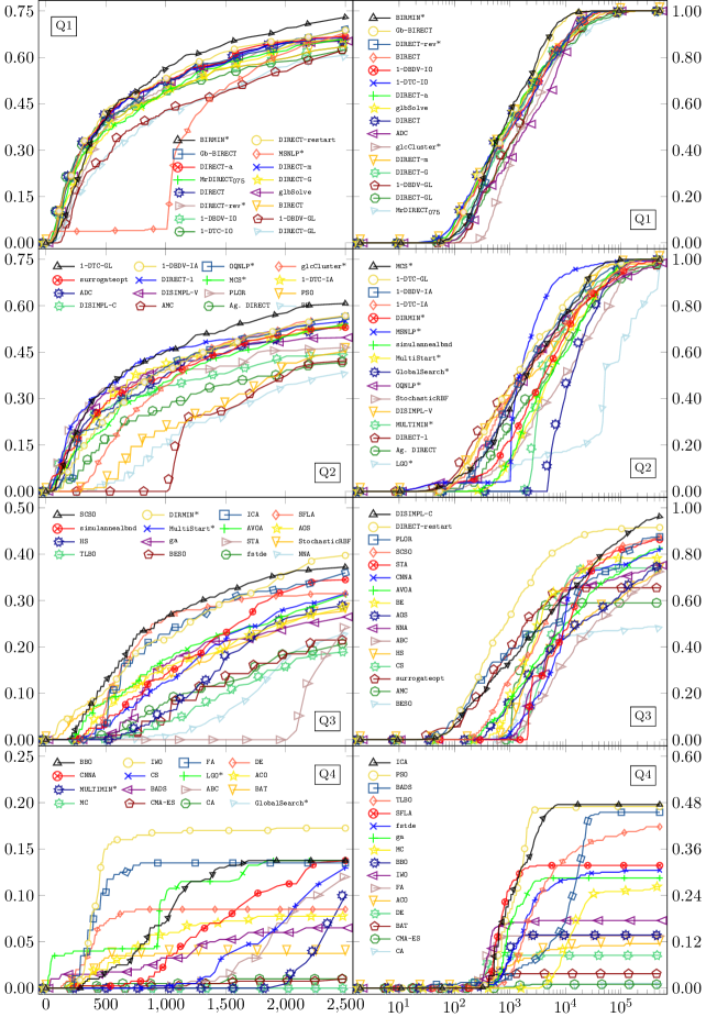
Figure 3: Data profiles: fraction of “simple” GKLS test problems solved within an allowable number of function evaluations show on the $x$-axis, while the $y$-axis shows the proportion of solved problems. On the left-side $M_{\rm max}=2,500$, while on the right-side $M_{\rm max}=500,000$ is used. Q1 shows the top-$16$ performing algorithms, Q2 the $17$th to $32$th places, Q3 the $33$st to $48$th, and Q4 the $49$th to $64$th.

The fourth and fifth columns in Table 7 presents the average number of execution time in seconds ($t_{\rm avg.}$) and standard deviation ($t_{\rm s.d.}$) for all $400$ “simple” GKLS-type problems using $M_{\rm max}=2,500$. Despite the poor performance of meta-heuristic algorithms based on the function evaluation criteria, they are often much faster than deterministic ones (see the fourth column in Table 7). Therefore, they can perform more function evaluations in the same time budget. The tree the fastest are the AVOA, CS, and CMA-ES algorithms. Among the fastest approaches, at least nine other approaches with an average speed of fewer than $0.1$ fractions of a second. Out of $64$ algorithms, only $18$ had an average time greater than one second. The model-based surrogateopt and BADS algorithms were the two slowest algorithms, of which the surrogateopt averaged more than one minute ($72.91$ s.).

4.1.2 Comparison on “simple” GKLS problems with $M_{\rm max}=500,000$

From seventh to eleventh columns in Table 7 shows the average number of function evaluations ($f_{\rm avg.}$), standard deviation ($f_{\rm s.d.}$), average time ($f_{\rm avg.}$), standard deviation ($t_{\rm s.d.}$), and success rate for all $400$ GKLS “simple” class test problems using $M_{\rm max}=500,000$. As the maximal budget for function evaluation increased significantly, the number of fails has accordingly decreased for most of the algorithms. Even $21$ algorithms out of $64$ demonstrated a perfect success rate (all are deterministic). However, even with $M_{\rm max}=500,000$, six hybridized algorithms (MSNLP*, OQNLP*, MultiStart*, LGO*, MULTIMIN*, and GlobalSearch*) suffered from a lack of success and surprisingly are significantly outperformed by the standard DIRECT-type algorithms. Again, quite surprisingly, increasing the budget for objective function evaluations for some algorithms (CA, DE, SFLA, IWO, BBO, FA, CMA-ES, and BAT) did not improve. The success ratio remained the same as within $M_{\rm max}=2,500$.

Again, the best average results were achieved using the hybridized BIRMIN* algorithm, closely followed by Gb-BIRECT. In contrast, the third DIRECT-rev* and fourth 1-DBDV-IO best algorithms deliver approximately $48\%$ and $52\%$ worse overall average number of function evaluations. Among the stochastic approaches, the best average results were achieved using simulannealbnd algorithm, but it ranks only in $23$rd place among all the best-performing algorithms. Another two algorithms dominating the stochastic pool are two hybridized MultiStart* and MULTIMIN* approaches, requiring approximately $91.75\%$ and $92.23\%$ more function evaluations than BIRMIN*. Also, when the number of function evaluations allowed is higher, twice as many stochastic algorithms make it into the top-$32$.

The data profiles on the right-side of Fig. 3 illustrate the performances of the algorithms within $M_{\rm max}=500,000$. The data profiles in the top right graph of Fig. 3 reveal that all the best algorithms in the Q1 category are DIRECT-type and perform very competitively. When the budget of function evaluation increases ($\geq 800$), the BIRMIN* algorithm gives slightly better performance efficiency and achieves an ideal success rate ($1.00$) within the $20,000$ budget. None of the $16$ Q1 algorithms needed more than $100,000$ function evaluations to reach the ideal success ratio. In the set of stochastic algorithms, the best performing algorithm was simulannealbnd, closely followed by MultiStart* and GlobalSearch*. All three stochastic algorithms were very close to the ideal success ratio ($0.99$), but the solvers needed to use a maximal budget ($M_{\rm max}=500,000$).

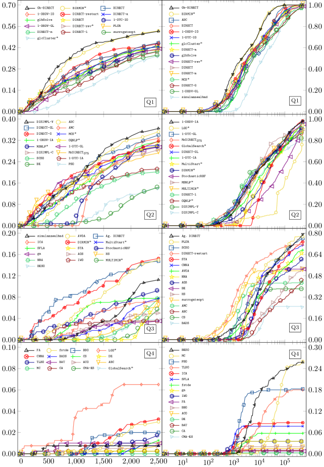
Figure 4: Data profiles: fraction of “hard” GKLS test problems solved within an allowable number of function evaluations show on the $x$-axis, while the $y$-axis shows the proportion of solved problems. On the left-side $M_{\rm max}=2,500$, while on the right-side $M_{\rm max}=500,000$ is used. Q1 shows the top-$16$ performing algorithms, Q2 the $17$th to $32$th places, Q3 the $33$st to $48$th, and Q4 the $49$th to $64$th.

Among the $64$ algorithms, 1-DTC-GL was the algorithm that solved all the problems fastest. Only fourteen algorithms managed to fit into the one minute. All approaches belong to the DIRECT-type class. As the budget for evaluating objective functions is significantly higher than $M_{\rm max}=2,500$, some algorithms have proven to be very inefficient with respect to running time. Model-based algorithms are clearly not the best choice for solving problems with large budgets for evaluating objective functions. The average time to solve $400$ “simple” class problems with the BADS algorithm is as high as $1,955.32$ seconds. The standard deviation shows that the algorithm is often terminated due to a violation of the time-limited ($M_{\rm max}=3,600$) stopping condition.

4.1.3 Comparison on “hard” GKLS problems with $M_{\rm max}=2,500$

The summarized results are shown in the second to sixth columns of Table 8. When the complexity increased, the performance efficiency significantly worsened, and the number of fails, was also increased. The BIRMIN* and Gb-BIRECT algorithms share the largest number ($214$) of solved test problems. Quite surprisingly the non-hybridized Gb-BIRECT algorithm requires approximately $3\%$ fewer objective function evaluations. The third and fourth-best algorithms were BIRECT and 1-DBDV-IO. Both solved slightly less than half ($184$) of these test problems within $M_{\rm max}=2,500$. Interestingly, the top four algorithms are based on the same partitioning scheme Paulavicius2016:jogo .

Among the stochastic algorithms, in the “hard” GKLS class, the surrogateopt algorithm is still the best but ranks only $15$th. The second and third best averages results and success rates were achieved by the AMC and SCSO stochastic algorithms. The remaining stochastic algorithms could not solve more than a fifth of these test problems within $M_{\rm max}=2,500$.

As in the previous study on $400$ “simple” test class GKLS problems, the fastest solvers (the lowest execution time) achieved with AVOA, CS, and CMA-ES.

Finally, the data profiles on the left side of Fig. 4 illustrate the performances of algorithms on “hard” problems up to $M_{\rm max}=2,500$. The best two solvers, BIRMIN* and Gb-BIRECT, share very similar performance and solved $54\%$ of test instances, followed by BIRECT and 1-DBDV-IO, which solved $46\%$. Among the stochastic algorithms, only the surrogateopt algorithm is the sole candidate in Q1. However, efficiency is one of the worst in this category.

4.1.4 Comparison on “hard” GKLS problems with $M_{\rm max}=500,000$

Finally, the seventh to tenth columns in Table 8 presents the average and standard deviation values of function evaluations and execution times, while the last column — success rate on all $400$ GKLS “hard” test problems using $M_{\rm max}=500,000$. Only six algorithms achieved a perfect success rate compared to $21$ for the “simple“ class. All of them are DIRECT-type algorithms. Once again, the two best-performing algorithms are BIRMIN* and Gb-BIRECT. The BIRMIN* required approximately $2.3$ and $2.5$ times fewer function evaluations than the third and fourth-best ADC and 1-DBDV-IO algorithms. The simulannealbnd approach ranks first among stochastic algorithms. However, compared to the best-performing BIRMIN* algorithm, it required approximately $92\%$ more objective function evaluations.

This time, the average execution time revealed that no one algorithm could make it into the one-second time interval within $500,000$. The top three algorithms (including Gb-BIRECT and BIRMIN*, which are the best performers in average function evaluations and success rates) had average times of just under two seconds.

Finally, data profiles on the right-side of Fig. 4 show the performance on “hard” GKLS up to $M_{\rm max}=500,000$. The two DIRECT-type algorithms (BIRMIN* and Gb-BIRECT) outperform the following best solvers in the Q1 group. As in the previous case, only one best stochastic algorithm (simulannealbnd) is in Q1.

4.2 Computational results solving DIRECTGOLib v1.2 test problems

Table 9 summarizes experimental results on $397$ test problems from DIRECTGOLib v1.2, where the best results are given in bold. As previously, the second to sixth columns presents the performance using with a low evaluation budget ($M_{\rm max}=2,500$), while from the seventh to eleventh columns show the performance when $M_{\rm max}=500,000$.

Table 9: The average number ($f_{\rm avg.}$) and standard deviation ($f_{\rm s.d.}$) of function evaluations, the average value ($t_{\rm avg.}$) and standard deviation ($t_{\rm s.d.}$) of execution time, and the success rate (S. R.) for DIRECTGOLib v1.2 test problems using $M_{\rm max}=2,500$ and $M_{\rm max}=500,000$.

Evaluation budget	$M_{\rm max}=2,500$					$M_{\rm max}=500,000$
Criteria	$f_{\rm avg.}$	$f_{\rm s.d.}$	$t_{\rm avg.}$	$t_{\rm s.d.}$	S. R.	$f_{\rm avg.}$	$f_{\rm s.d.}$	$t_{\rm avg.}$	$t_{\rm s.d.}$	S. R.
AVOA	$\mathbf{1,263}$	$180$	$0.04$	$0.17$	$\mathbf{0.62}$	$\mathbf{113,651}$	$9,305$	$1.67$	$3.73$	$\mathbf{0.80}$
OQNLP*	$1,315$	$-$	$0.68$	$-$	$0.54$	$149,927$	$-$	$52.03$	$-$	$0.73$
MCS*	$1,389$	$-$	$7.01$	$-$	$0.53$	$166,738$	$-$	$930.09$	$-$	$0.68$
BESO	$1,498$	$56$	$0.15$	$0.11$	$0.49$	$178,163$	$21,669$	$14.43$	$23.13$	$0.67$
SCSO	$1,458$	$110$	$0.19$	$0.17$	$0.52$	$189,452$	$12,209$	$21.92$	$42.57$	$0.63$
MSNLP*	$1,480$	$-$	$0.78$	$-$	$0.50$	$188,425$	$-$	$66.77$	$-$	$0.64$
LGO*	$1,528$	$-$	$2.25$	$-$	$0.44$	$207,080$	$-$	$44.53$	$-$	$0.62$
DIRMIN*	$1,601$	$-$	$0.89$	$-$	$0.43$	$202,417$	$-$	$70.78$	$-$	$0.61$
BIRMIN*	$1,529$	$-$	$8.98$	$-$	$0.46$	$218,943$	$-$	$1,376.18$	$-$	$0.57$
fstde	$1,770$	$61$	$0.46$	$0.28$	$0.38$	$185,126$	$12,402$	$45.49$	$72.16$	$0.65$
1-DTC-GL	$1,747$	$-$	$1.92$	$-$	$0.37$	$192,664$	$-$	$192.28$	$-$	$0.66$
DIRECT-rev*	$1,597$	$-$	$18.08$	$-$	$0.45$	$221,212$	$-$	$1,395.02$	$-$	$0.57$
AOS	$1,667$	$106$	$0.12$	$0.08$	$0.45$	$227,009$	$18,453$	$12.41$	$14.18$	$0.57$
CA	$1,536$	$157$	$0.64$	$0.48$	$0.48$	$239,902$	$23,049$	$97.59$	$165.04$	$0.52$
1-DBDV-GL	$1,838$	$-$	$1.26$	$-$	$0.33$	$199,097$	$-$	$104.76$	$-$	$0.66$
MultiStart*	$1,705$	$97$	$0.26$	$0.18$	$0.40$	$225,333$	$8,417$	$27.15$	$54.90$	$0.57$
1-DTC-IA	$1,799$	$-$	$0.87$	$-$	$0.35$	$213,808$	$-$	$64.89$	$-$	$0.62$
1-DBDV-IA	$1,836$	$-$	$0.91$	$-$	$0.34$	$216,331$	$-$	$60.69$	$-$	$0.62$
STA	$2,421$	$31$	$0.35$	$1.78$	$0.27$	$169,599$	$21,235$	$1.94$	$3.92$	$0.69$
1-DBDV-IO	$1,713$	$-$	$7.71$	$-$	$0.39$	$224,606$	$-$	$1,079.43$	$-$	$0.56$
1-DTC-IO	$1,704$	$-$	$8.69$	$-$	$0.38$	$241,479$	$-$	$1,288.62$	$-$	$0.53$
DIRECT-GL	$1,860$	$-$	$0.47$	$-$	$0.31$	$222,408$	$-$	$14.82$	$-$	$0.59$
PLOR	$1,800$	$-$	$2.15$	$-$	$0.34$	$233,973$	$-$	$251.50$	$-$	$0.55$
ACO	$1,861$	$81$	$1.16$	$0.76$	$0.35$	$237,220$	$20,908$	$157.31$	$246.80$	$0.54$
BADS	$1,576$	$141$	$454.06$	$356.54$	$0.44$	$276,024$	$10,680$	$2,007.41$	$1,754.28$	$0.45$
TLBO	$1,958$	$68$	$0.20$	$0.10$	$0.32$	$238,584$	$20,726$	$19.92$	$25.90$	$0.56$
DE	$1,834$	$96$	$0.52$	$0.29$	$0.35$	$243,004$	$36,269$	$63.24$	$76.15$	$0.53$
CNNA	$2,151$	$84$	$0.13$	$0.06$	$0.19$	$187,284$	$13,095$	$8.05$	$12.16$	$0.68$
SFLA	$1,872$	$80$	$0.58$	$0.37$	$0.35$	$245,699$	$27,318$	$77.09$	$127.82$	$0.52$
DIRECT-G	$1,871$	$-$	$0.44$	$-$	$0.31$	$243,025$	$-$	$14.61$	$-$	$0.55$
glbSolve	$1,855$	$-$	$1.78$	$-$	$0.30$	$250,617$	$-$	$204.10$	$-$	$0.56$
PSO	$2,046$	$75$	$0.31$	$0.13$	$0.29$	$227,322$	$27,376$	$29.57$	$31.69$	$0.56$
glcCluster*	$2,108$	$-$	$13.61$	$-$	$0.25$	$205,664$	$-$	$1,455.86$	$-$	$0.59$
ICA	$2,016$	$73$	$0.68$	$0.32$	$0.28$	$235,327$	$22,066$	$76.64$	$82.83$	$0.54$
NNA	$2,262$	$62$	$0.20$	$0.07$	$0.14$	$182,670$	$17,531$	$12.70$	$26.55$	$0.67$
ga	$2,020$	$115$	$0.16$	$0.08$	$0.27$	$247,560$	$35,022$	$15.23$	$20.07$	$0.54$
CS	$2,213$	$66$	$0.09$	$0.05$	$0.18$	$219,341$	$10,682$	$5.49$	$7.76$	$0.62$
DIRECT-l	$1,835$	$-$	$9.62$	$-$	$0.31$	$274,955$	$-$	$1,446.93$	$-$	$0.47$
BBO	$1,953$	$121$	$1.28$	$0.69$	$0.31$	$263,791$	$29,302$	$174.24$	$233.95$	$0.47$
BIRECT	$1,840$	$-$	$4.31$	$-$	$0.32$	$280,776$	$-$	$644.96$	$-$	$0.45$
FA	$1,957$	$104$	$0.36$	$0.11$	$0.28$	$257,724$	$26,112$	$38.75$	$37.66$	$0.49$
Gb-BIRECT	$1,864$	$-$	$6.02$	$-$	$0.31$	$284,990$	$-$	$914.77$	$-$	$0.45$
GlobalSearch*	$2,470$	$12$	$0.21$	$0.04$	$0.11$	$198,720$	$14,353$	$13.44$	$20.18$	$0.65$
MrDIRECT${}_{\text{075}}$	$1,875$	$-$	$1.53$	$-$	$0.29$	$281,020$	$-$	$180.80$	$-$	$0.46$
Ag. DIRECT	$1,991$	$-$	$0.47$	$-$	$0.26$	$276,015$	$-$	$10.69$	$-$	$0.48$
HS	$2,078$	$99$	$0.52$	$0.23$	$0.24$	$268,195$	$16,769$	$63.72$	$67.14$	$0.50$
BE	$2,102$	$77$	$0.40$	$0.10$	$0.24$	$262,122$	$16,767$	$39.29$	$38.12$	$0.49$
surrogateopt	$1,714$	$74$	$387.54$	$313.01$	$0.35$	$316,040$	$5,711$	$2,367.07$	$1,654.37$	$0.37$
DIRECT	$1,900$	$-$	$1.61$	$-$	$0.28$	$284,593$	$-$	$195.63$	$-$	$0.44$
DIRECT-m	$1,893$	$-$	$7.58$	$-$	$0.28$	$286,145$	$-$	$112.62$	$-$	$0.44$
DIRECT-restart	$1,857$	$-$	$6.32$	$-$	$0.30$	$295,712$	$-$	$1,001.60$	$-$	$0.42$
CMA-ES	$2,025$	$69$	$0.29$	$0.24$	$0.27$	$285,322$	$27,388$	$36.74$	$63.86$	$0.45$
AMC	$2,048$	$91$	$0.16$	$0.07$	$0.26$	$283,518$	$16,866$	$16.50$	$23.23$	$0.44$
DIRECT-a	$1,905$	$-$	$3.32$	$-$	$0.28$	$303,547$	$-$	$160.28$	$-$	$0.41$
StochasticRBF	$1,838$	$47$	$19.20$	$76.18$	$0.30$	$316,717$	$2,573$	$2,285.50$	$1,715.81$	$0.37$
IWO	$2,111$	$88$	$0.31$	$0.13$	$0.22$	$281,501$	$26,616$	$36.92$	$32.58$	$0.45$
ABC	$2,213$	$67$	$0.41$	$0.14$	$0.17$	$276,920$	$4,196$	$45.86$	$40.19$	$0.49$
ADC	$1,876$	$-$	$13.20$	$-$	$0.29$	$326,049$	$-$	$2,348.85$	$-$	$0.35$
DISIMPL-V	$1,938$	$-$	$1,996.45$	$-$	$0.26$	$323,428$	$-$	$2,335.31$	$-$	$0.36$
MULTIMIN*	$2,425$	$15$	$0.17$	$0.04$	$0.07$	$238,069$	$12,135$	$11.99$	$15.84$	$0.53$
simulannealbnd	$2,046$	$87$	$1.14$	$0.51$	$0.23$	$328,016$	$9,129$	$177.11$	$181.02$	$0.36$
DISIMPL-C	$2,009$	$-$	$1,997.31$	$-$	$0.22$	$349,459$	$-$	$2,256.41$	$-$	$0.32$
BAT	$2,008$	$122$	$0.06$	$0.04$	$0.25$	$369,555$	$28,028$	$4.55$	$4.28$	$0.26$
MC	$2,319$	$61$	$0.16$	$0.05$	$0.10$	$402,594$	$11,360$	$19.98$	$15.86$	$0.22$

Unlike in Section 4.1, where deterministic algorithms dominate over stochastic, the stochastic solvers are very competitive and often perform better. There have been five algorithms (AVOA, OQNLP*, MCS*, SCSO, and MSNLP*) that managed to achieve a success rate of $\geq 0.5$ within $M_{\rm max}=2,500$. Moreover, nine algorithms (AVOA, OQNLP*, STA, MCS*, CNNA, AMC, BESO, 1-DTC-GL, and 1-DBDV-GL) were able to solve at least two-thirds of the test problems when $M_{\rm max}=500,000$. Among all problems, the meta-heuristic nature-inspired AVOA algorithm showed the best performance in both cases (for $M_{\rm max}=2,500$, and $M_{\rm max}=500,000$). The success rates of the AVOA algorithm (in the $M_{\rm max}=2,500$ and $M_{\rm max}=500,000$ cases) are $62\%$ and $80\%$. The AVOA also proves to be the fastest when comparing the average execution time.

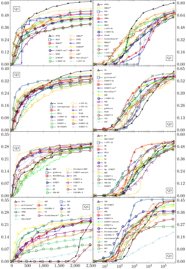
Figure 5: Data profiles: fraction of $397$ DIRECTGOLib v1.2 test problems solved as a function of allowable number of function evaluation. The horizontal coordinate equals a number of function evaluations or median value while the vertical coordinate equals a proportion of solved problems. The evaluation budget on the left is $2,500$, while on the right it is $500,000$. Also Q1 shows the top-$16$ performing algorithms, Q2 the $17$th to $32$th place, Q3 the $33$st to $48$th and Q4 the $49$th to $64$th.

The data profiles on the left-side of Fig. 5 illustrate the performance of algorithms up to $M_{\rm max}=2,500$. When the budget is meager ($\leq 500$), the best performing algorithms are OQNLP* and MCS* and solved approximately $45\%$ of all problems from DIRECTGOLib v1.2. However, when the budget increases ($>500$), the AVOA algorithm starts outperforming others. Among the top-$32$ solvers, fifteen are DIRECT-type, while ten are meta-heuristics.

Many hybridized algorithms did not perform well in the previous Section 4.1. However, lots of the DIRECTGOLib v1.2 test problems’ dimensions are much higher than the GKLS, and the hybridized solvers performed much better this time. Among the sixteen best-performing algorithms (Q1), eight are hybridized.

The data profiles on the right-side of Fig. 5 illustrate the performances using $M_{\rm max}=500,000$. The best two performing algorithms are the AVOA and OQNLP*. Using a higher budget, the efficiency of non-hybridized solvers has improved significantly. Now eleven out of the top sixteen algorithms are non-hybridized. Only six of the sixteen algorithms made into the Q1 when $M_{\rm max}=2,500$ remained here using $M_{\rm max}=500,000$.

Additionally, data profiles in Figs. 6, 7, 8 and 9 demonstrate a more detailed performance of the algorithms on different subsets of the DIRECTGOLib v1.2. The first observation is that four algorithms always make it into the Q1 — AVOA, OQNLP*, MCS*, and MSNLP*. The AVOA algorithm demonstrated the most significant advantage in solving high-dimensional, multi-modal, and non-convex test problems. On simpler uni-modal and/or convex test problems, the LGO* was the best performing algorithm, followed closely by OQNLP*, AVOA, and STA. For low-dimensional test problems, the best results are obtained using DIRECT-type algorithms, especially when $M_{\rm max}=500,000$.

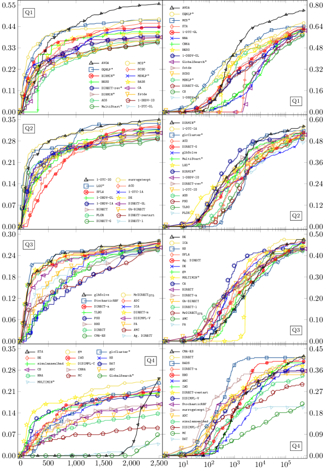
Figure 6: Data profiles: fraction of $320$ multi-modal and/or non-convex DIRECTGOLib v1.2 test problems solved within an allowable number of function evaluations show on the $x$-axis, while the $y$-axis shows the proportion of solved problems. On the left-side $M_{\rm max}=2,500$, while on the right-side $M_{\rm max}=500,000$ is used. Q1 shows the top-$16$ performing algorithms, Q2 the $17$th to $32$th places, Q3 the $33$st to $48$th, and Q4 the $49$th to $64$th.

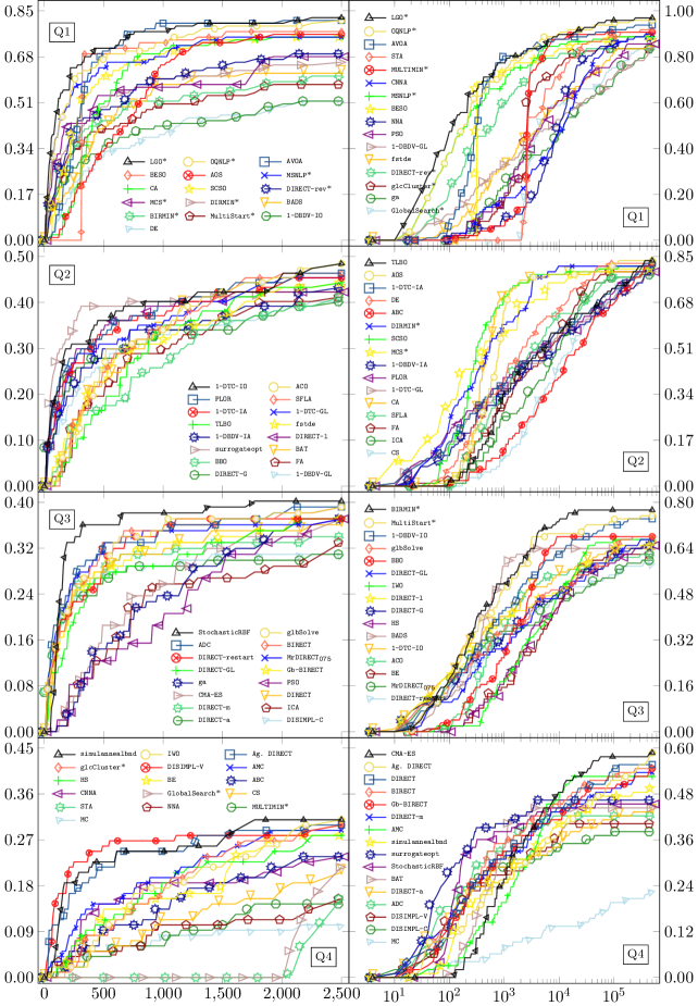
Figure 7: Data profiles: fraction of $97$ uni-modal and/or convex DIRECTGOLib v1.2 test problems solved within an allowable number of function evaluations show on the $x$-axis, while the $y$-axis shows the proportion of solved problems. On the left-side $M_{\rm max}=2,500$, while on the right-side $M_{\rm max}=500,000$ is used. Q1 shows the top-$16$ performing algorithms, Q2 the $17$th to $32$th places, Q3 the $33$st to $48$th, and Q4 the $49$th to $64$th.

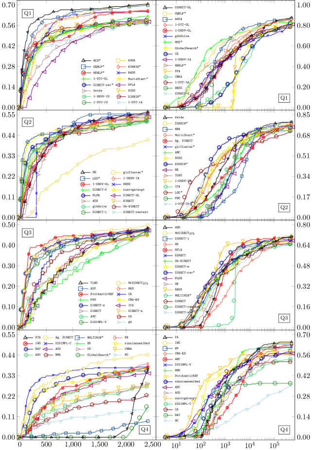
Figure 8: Data profiles: fraction of $231$ low-dimensional ($n\leq 10$) DIRECTGOLib v1.2 test problems solved within an allowable number of function evaluations show on the $x$-axis, while the $y$-axis shows the proportion of solved problems. On the left-side $M_{\rm max}=2,500$, while on the right-side $M_{\rm max}=500,000$ is used. Q1 shows the top-$16$ performing algorithms, Q2 the $17$th to $32$th places, Q3 the $33$st to $48$th, and Q4 the $49$th to $64$th.

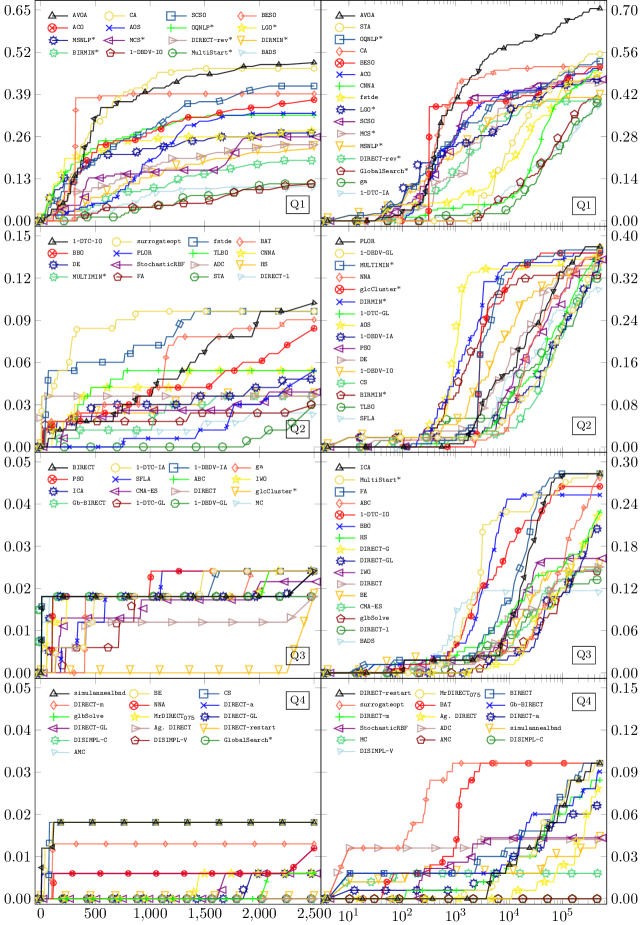
Figure 9: Data profiles: fraction of $166$ high-dimensional ($n>10$) DIRECTGOLib v1.2 test problems solved within an allowable number of function evaluations show on the $x$-axis, while the $y$-axis shows the proportion of solved problems. On the left-side $M_{\rm max}=2,500$, while on the right-side $M_{\rm max}=500,000$ is used. Q1 shows the top-$16$ performing algorithms, Q2 the $17$th to $32$th places, Q3 the $33$st to $48$th, and Q4 the $49$th to $64$th.

Table 10: The average number of function evaluations ($f_{\rm avg.}$), standard deviation (S. D.), and success rate (S. R.) when the solution is: at zero-point ($122$ cases), and at other non-zero locations ($198$ cases).

Evaluation budget	$M_{\rm max}=2,500$				$M_{\rm max}=500,000$
Minimum location	Zero-point		Non-zero		Zero-point		Non-zero
Criteria	$f_{\rm avg.}$	S. R.	$f_{\rm avg.}$	S. R.	$f_{\rm avg.}$	S. R.	$f_{\rm avg.}$	S. R.
AVOA	$972$	$0.81$	$1,671$	$0.40$	$21,239$	$0.97$	$198,287$	$0.63$
OQNLP*	$1,525$	$0.47$	$1,423$	$0.47$	$157,898$	$0.72$	$196,557$	$0.63$
MCS*	$1,508$	$0.47$	$1,432$	$0.50$	$168,392$	$0.69$	$194,373$	$0.62$
SCSO	$1,207$	$0.70$	$1,842$	$0.31$	$109,500$	$0.80$	$272,537$	$0.46$
BESO	$1,237$	$0.62$	$1,914$	$0.30$	$143,461$	$0.76$	$243,672$	$0.53$
MSNLP*	$1,677$	$0.42$	$1,615$	$0.44$	$226,343$	$0.56$	$215,091$	$0.59$
fstde	$1,882$	$0.36$	$1,751$	$0.36$	$191,994$	$0.67$	$222,718$	$0.56$
1-DTC-GL	$1,863$	$0.33$	$1,727$	$0.37$	$225,135$	$0.58$	$193,966$	$0.65$
DIRMIN*	$1,658$	$0.42$	$1,741$	$0.36$	$206,652$	$0.61$	$240,291$	$0.53$
STA	$2,433$	$0.32$	$2,398$	$0.26$	$143,206$	$0.76$	$231,138$	$0.56$
BIRMIN*	$1,647$	$0.40$	$1,534$	$0.46$	$252,237$	$0.51$	$237,463$	$0.53$
CA	$1,359$	$0.62$	$1,917$	$0.26$	$173,093$	$0.67$	$339,296$	$0.30$
1-DBDV-GL	$1,904$	$0.30$	$1,839$	$0.33$	$236,293$	$0.57$	$207,497$	$0.64$
DIRECT-rev*	$1,714$	$0.39$	$1,702$	$0.39$	$231,957$	$0.55$	$261,467$	$0.48$
AOS	$1,771$	$0.45$	$1,847$	$0.32$	$233,569$	$0.57$	$275,762$	$0.46$
1-DBDV-IA	$1,906$	$0.30$	$1,846$	$0.33$	$250,008$	$0.55$	$229,805$	$0.59$
LGO*	$1,594$	$0.41$	$1,862$	$0.30$	$247,416$	$0.54$	$260,493$	$0.52$
MultiStart*	$1,941$	$0.33$	$1,687$	$0.38$	$260,109$	$0.52$	$236,205$	$0.53$
1-DTC-IA	$1,949$	$0.30$	$1,794$	$0.34$	$266,705$	$0.52$	$224,916$	$0.59$
ACO	$1,907$	$0.35$	$1,908$	$0.32$	$223,801$	$0.59$	$255,436$	$0.49$
DIRECT-GL	$1,955$	$0.26$	$1,827$	$0.33$	$246,293$	$0.56$	$221,610$	$0.59$
1-DBDV-IO	$1,842$	$0.31$	$1,725$	$0.39$	$259,482$	$0.50$	$242,540$	$0.53$
1-DTC-IO	$1,783$	$0.34$	$1,731$	$0.36$	$242,585$	$0.52$	$262,260$	$0.48$
CNNA	$2,238$	$0.20$	$2,146$	$0.17$	$188,573$	$0.71$	$232,406$	$0.56$
DIRECT-G	$1,999$	$0.25$	$1,846$	$0.32$	$267,858$	$0.52$	$248,495$	$0.54$
BADS	$1,486$	$0.42$	$1,645$	$0.39$	$246,506$	$0.43$	$298,821$	$0.39$
glbSolve	$1,973$	$0.26$	$1,852$	$0.30$	$283,702$	$0.48$	$260,338$	$0.55$
NNA	$2,286$	$0.15$	$2,243$	$0.14$	$124,519$	$0.72$	$227,581$	$0.56$
glcCluster*	$2,205$	$0.21$	$2,078$	$0.26$	$215,249$	$0.57$	$245,672$	$0.52$
TLBO	$2,102$	$0.29$	$1,960$	$0.29$	$283,226$	$0.49$	$261,589$	$0.48$
SFLA	$1,966$	$0.34$	$1,901$	$0.30$	$281,684$	$0.47$	$275,514$	$0.44$
PSO	$2,127$	$0.28$	$2,042$	$0.27$	$266,552$	$0.51$	$259,321$	$0.48$
PLOR	$1,987$	$0.25$	$1,819$	$0.32$	$270,034$	$0.48$	$268,858$	$0.48$
DE	$1,804$	$0.30$	$1,858$	$0.31$	$195,629$	$0.48$	$279,593$	$0.44$
CS	$2,271$	$0.18$	$2,183$	$0.18$	$255,804$	$0.59$	$232,084$	$0.57$
ICA	$2,020$	$0.29$	$2,012$	$0.26$	$200,028$	$0.49$	$262,589$	$0.47$
ga	$2,079$	$0.28$	$2,038$	$0.24$	$262,609$	$0.53$	$286,766$	$0.44$
BIRECT	$1,937$	$0.26$	$1,831$	$0.33$	$297,452$	$0.43$	$285,983$	$0.43$
Gb-BIRECT	$1,978$	$0.25$	$1,825$	$0.34$	$315,525$	$0.39$	$278,499$	$0.45$
GlobalSearch*	$2,486$	$0.10$	$2,476$	$0.07$	$215,610$	$0.66$	$219,102$	$0.59$
BE	$2,112$	$0.25$	$2,095$	$0.22$	$239,363$	$0.49$	$279,700$	$0.45$
HS	$2,048$	$0.25$	$2,101$	$0.20$	$231,553$	$0.54$	$296,494$	$0.42$
DIRECT-l	$1,886$	$0.25$	$1,795$	$0.31$	$277,431$	$0.39$	$273,043$	$0.45$
BBO	$1,915$	$0.29$	$1,982$	$0.26$	$217,463$	$0.45$	$299,572$	$0.39$
Ag. DIRECT	$2,108$	$0.20$	$1,941$	$0.29$	$314,032$	$0.39$	$265,116$	$0.51$
MrDIRECT${}_{\text{075}}$	$1,999$	$0.25$	$1,854$	$0.30$	$314,277$	$0.39$	$282,801$	$0.44$
surrogateopt	$1,655$	$0.35$	$1,760$	$0.33$	$301,918$	$0.36$	$326,946$	$0.34$
DIRECT-m	$1,991$	$0.25$	$1,870$	$0.28$	$305,262$	$0.40$	$285,227$	$0.44$
AMC	$2,178$	$0.25$	$1,994$	$0.26$	$295,270$	$0.44$	$287,711$	$0.42$
DIRECT-a	$1,989$	$0.25$	$1,871$	$0.29$	$308,132$	$0.40$	$298,698$	$0.41$
FA	$1,934$	$0.27$	$1,975$	$0.25$	$219,650$	$0.41$	$287,129$	$0.42$
DIRECT	$1,980$	$0.25$	$1,920$	$0.26$	$292,914$	$0.43$	$301,685$	$0.41$
CMA-ES	$2,021$	$0.25$	$2,028$	$0.25$	$277,697$	$0.39$	$291,212$	$0.44$
DIRECT-restart	$1,988$	$0.24$	$1,827$	$0.32$	$335,458$	$0.34$	$300,210$	$0.40$
StochasticRBF	$1,877$	$0.24$	$1,807$	$0.30$	$321,375$	$0.33$	$313,119$	$0.37$
DISIMPL-V	$1,993$	$0.23$	$1,916$	$0.28$	$339,460$	$0.33$	$312,807$	$0.38$
ADC	$1,960$	$0.25$	$1,891$	$0.30$	$345,790$	$0.31$	$321,908$	$0.36$
IWO	$2,117$	$0.22$	$2,106$	$0.20$	$251,732$	$0.39$	$304,491$	$0.39$
simulannealbnd	$2,018$	$0.24$	$2,068$	$0.19$	$319,207$	$0.35$	$334,819$	$0.33$
ABC	$2,218$	$0.17$	$2,209$	$0.15$	$251,156$	$0.38$	$296,818$	$0.40$
MULTIMIN*	$2,483$	$0.08$	$2,462$	$0.02$	$270,024$	$0.50$	$293,981$	$0.40$
DISIMPL-C	$2,109$	$0.18$	$2,017$	$0.22$	$373,221$	$0.27$	$343,926$	$0.33$
BAT	$1,969$	$0.20$	$2,039$	$0.21$	$356,268$	$0.20$	$379,817$	$0.22$
MC	$2,319$	$0.13$	$2,320$	$0.07$	$411,733$	$0.22$	$395,536$	$0.22$

4.2.1 Investigating the impact of the solution lying at zero

Despite the outstanding performance of the AVOA and some other meta-heuristic algorithms, there is one crucial point that needs additional discussion. It is natural to assume that the algorithms are unbiased to the landscape of problems. However, during these experiments, it has been observed that some approaches give extra attention to exploring the region around the zero point. Of $397$ test problems, $173$ had solutions precisely at the zero point, and $122$ of these test problems were highly complex. Therefore, an additional study was carried out, and the results are summarized in Table 10. Here we have selected two subgroups depending on where the solutions are: highly complex problems with solutions at the zero point ($122$ cases) and all problems with a solution at other locations ($198$ cases).

Standard non-hybridized DIRECT-type algorithms make almost no difference whether the global solution is at the zero point or elsewhere. Furthermore, non-hybridized DIRECT-type solvers often perform better when the global solution is at a non-zero point. For example, the Ag. DIRECT algorithm manages to achieve $31\%$ greater success rate on non-zero problems using $M_{\rm max}=2,500$, and about $23\%$ when $M_{\rm max}=500,000$.

The results of the hybridized algorithms are also very similar. Some algorithms work slightly better when the global solution is at the zero point, and in some cases, the opposite is true. Seven (out of eleven) hybridized algorithms better solved non-zero problems. When $M_{\rm max}=2,500$, the best performing algorithm on non-zero problems is MCS*, followed by OQNLP* and BIRMIN* algorithms. When $M_{\rm max}=500,000$, the best results were achieved using the OQNLP* algorithm, closely followed by the MCS* and MSNLP*. However, in overall rating, the standard non-hybridized algorithms (1-DTC-GL and 1-DBDV-GL) proved to be better at solving non-zero problems, especially when $M_{\rm max}=500,000$.

The AVOA algorithm, which showed outstanding results in Table 9, does not perform so well on non-zero problems. When $M_{\rm max}=2,500$, AVOA is outperformed by four algorithms, while when $M_{\rm max}=500,000$, it shares the third-fourth places. Completely different results are obtained with the AVOA algorithm on $122$ zero-point test problems. Using $M_{\rm max}=2,500$, the success ratio of the AVOA algorithm is $0.81$, i.e., more than twice that higher compared the success ratio ($0.40$) on non-zero problems. When $M_{\rm max}=500,000$, the AVOA success ratio (on zero-point problems) was close to the ideal ($0.97$), while on non-zero problems, it reached only $0.63$. The AVOA algorithm required about $89\%$ fewer objective function evaluations on zero-point problems. Thus, even the AVOA algorithm’s initial population is generated randomly over $D$, but the algorithm naturally tends to converge to a zero-point.

Similar behavior has been observed for more meta-heuristic algorithms, such as SCSO, AOS, BESO, CNNA, CA, and STA. Using $M_{\rm max}=2,500$ nine algorithms achieved more than $25\%$ greater a success rate on zero-point problems. Eight of these nine algorithms are stochastic, and most of them ($5$) are population-based search (PBS) techniques. Similar trends persisted using $M_{\rm max}=500,000$.

5 Summary of numerical benchmarking

Two extensive different analyses on GKLS and DIRECTGOLib v1.2 test datasets did not reveal a clear dominant algorithm. On the contrary, it has revealed rather conflicting results. While deterministic (especially DIRECT-type) algorithms performed better in solving GKLS-generated test problems, various stochastic algorithms dominated and performed better in solving DIRECTGOLib v1.2 test problems. Therefore, to summarize all experimental results, we calculated the average success rates of all algorithms in Table 11. Here, the second and fifth columns show the average success rates on all GKLS problems using two different budgets, while the third and sixth columns show on DIRECTGOLib v1.2 test problems. The fourth and seventh columns present the combined average success rates on all $1,197$ test problems for each budget separately. Finally, the eighth column gives the overall average used to rank all considered algorithms.

Table 11: The average number of success rates using different test sets and evaluation budgets.

Evaluation budget	$M_{\rm max}=2,500$			$M_{\rm max}=500,000$
Test set	GKLS	DIRECTGOLib	Average	GKLS	DIRECTGOLib	Average	Overall average
BIRMIN*	$0.64$	$0.46$	$0.55$	$1.00$	$0.57$	$0.79$	$0.67$
OQNLP*	$0.44$	$0.54$	$0.49$	$0.93$	$0.73$	$0.83$	$0.66$
MCS*	$0.44$	$0.53$	$0.48$	$0.99$	$0.68$	$0.84$	$0.66$
MSNLP*	$0.50$	$0.50$	$0.50$	$0.94$	$0.64$	$0.79$	$0.65$
DIRECT-rev*	$0.54$	$0.45$	$0.50$	$1.00$	$0.57$	$0.78$	$0.64$
1-DBDV-GL	$0.53$	$0.33$	$0.43$	$0.99$	$0.66$	$0.83$	$0.63$
1-DBDV-IO	$0.55$	$0.39$	$0.47$	$1.00$	$0.56$	$0.78$	$0.63$
1-DTC-GL	$0.46$	$0.37$	$0.41$	$0.99$	$0.66$	$0.82$	$0.62$
1-DTC-IO	$0.54$	$0.38$	$0.46$	$1.00$	$0.53$	$0.77$	$0.61$
AVOA	$0.26$	$0.62$	$0.44$	$0.74$	$0.80$	$0.77$	$0.60$
glbSolve	$0.55$	$0.30$	$0.43$	$1.00$	$0.56$	$0.78$	$0.60$
1-DBDV-IA	$0.45$	$0.34$	$0.40$	$0.99$	$0.62$	$0.81$	$0.60$
Gb-BIRECT	$0.62$	$0.31$	$0.46$	$1.00$	$0.45$	$0.73$	$0.59$
DIRECT-GL	$0.49$	$0.31$	$0.40$	$0.98$	$0.59$	$0.78$	$0.59$
DIRECT-G	$0.50$	$0.31$	$0.40$	$0.99$	$0.55$	$0.77$	$0.59$
BIRECT	$0.55$	$0.32$	$0.44$	$1.00$	$0.45$	$0.73$	$0.58$
1-DTC-IA	$0.38$	$0.35$	$0.37$	$0.97$	$0.62$	$0.80$	$0.58$
glcCluster*	$0.48$	$0.25$	$0.36$	$1.00$	$0.59$	$0.79$	$0.58$
DIRMIN*	$0.28$	$0.43$	$0.36$	$0.97$	$0.61$	$0.79$	$0.57$
SCSO	$0.32$	$0.52$	$0.42$	$0.81$	$0.63$	$0.72$	$0.57$
DIRECT	$0.55$	$0.28$	$0.42$	$1.00$	$0.44$	$0.72$	$0.57$
DIRECT-m	$0.54$	$0.28$	$0.41$	$1.00$	$0.44$	$0.72$	$0.56$
DIRECT-a	$0.56$	$0.28$	$0.42$	$1.00$	$0.41$	$0.70$	$0.56$
MrDIRECT${}_{\text{075}}$	$0.48$	$0.29$	$0.38$	$0.99$	$0.46$	$0.72$	$0.55$
MultiStart*	$0.26$	$0.40$	$0.33$	$0.97$	$0.57$	$0.77$	$0.55$
DIRECT-l	$0.48$	$0.31$	$0.39$	$0.93$	$0.47$	$0.70$	$0.55$
PLOR	$0.44$	$0.34$	$0.39$	$0.83$	$0.55$	$0.69$	$0.54$
LGO*	$0.10$	$0.44$	$0.27$	$0.98$	$0.62$	$0.80$	$0.54$
DIRECT-restart	$0.58$	$0.30$	$0.44$	$0.82$	$0.42$	$0.62$	$0.53$
ADC	$0.45$	$0.29$	$0.37$	$1.00$	$0.35$	$0.68$	$0.52$
STA	$0.23$	$0.27$	$0.25$	$0.78$	$0.69$	$0.74$	$0.49$
DISIMPL-V	$0.44$	$0.26$	$0.35$	$0.90$	$0.36$	$0.63$	$0.49$
AOS	$0.22$	$0.45$	$0.33$	$0.70$	$0.57$	$0.63$	$0.48$
Ag. DIRECT	$0.29$	$0.26$	$0.28$	$0.89$	$0.48$	$0.68$	$0.48$
simulannealbnd	$0.27$	$0.23$	$0.25$	$0.99$	$0.36$	$0.67$	$0.46$
StochasticRBF	$0.22$	$0.30$	$0.26$	$0.96$	$0.37$	$0.67$	$0.46$
DISIMPL-C	$0.38$	$0.22$	$0.30$	$0.89$	$0.32$	$0.61$	$0.45$
surrogateopt	$0.48$	$0.35$	$0.41$	$0.61$	$0.37$	$0.49$	$0.45$
GlobalSearch*	$0.00$	$0.11$	$0.06$	$0.98$	$0.65$	$0.81$	$0.43$
CNNA	$0.11$	$0.19$	$0.15$	$0.76$	$0.68$	$0.72$	$0.43$
BE	$0.32$	$0.24$	$0.28$	$0.68$	$0.49$	$0.58$	$0.43$
BESO	$0.16$	$0.49$	$0.33$	$0.40$	$0.67$	$0.53$	$0.43$
NNA	$0.16$	$0.14$	$0.15$	$0.71$	$0.67$	$0.69$	$0.42$
MULTIMIN*	$0.11$	$0.07$	$0.09$	$0.93$	$0.53$	$0.73$	$0.41$
AMC	$0.40$	$0.26$	$0.33$	$0.52$	$0.44$	$0.48$	$0.40$
HS	$0.22$	$0.24$	$0.23$	$0.63$	$0.50$	$0.57$	$0.40$
PSO	$0.33$	$0.29$	$0.31$	$0.36$	$0.56$	$0.46$	$0.38$
CS	$0.10$	$0.18$	$0.14$	$0.55$	$0.62$	$0.58$	$0.36$
ICA	$0.27$	$0.28$	$0.28$	$0.34$	$0.54$	$0.44$	$0.36$
fstde	$0.16$	$0.38$	$0.27$	$0.24$	$0.65$	$0.45$	$0.36$
SFLA	$0.25$	$0.35$	$0.30$	$0.25$	$0.52$	$0.39$	$0.34$
TLBO	$0.15$	$0.32$	$0.23$	$0.33$	$0.56$	$0.45$	$0.34$
BADS	$0.08$	$0.44$	$0.26$	$0.40$	$0.45$	$0.42$	$0.34$
ABC	$0.07$	$0.17$	$0.12$	$0.59$	$0.49$	$0.54$	$0.33$
ga	$0.21$	$0.27$	$0.24$	$0.22$	$0.54$	$0.38$	$0.31$
ACO	$0.09$	$0.35$	$0.22$	$0.13$	$0.54$	$0.33$	$0.28$
DE	$0.10$	$0.35$	$0.22$	$0.10$	$0.53$	$0.31$	$0.27$
BBO	$0.14$	$0.31$	$0.23$	$0.14$	$0.47$	$0.31$	$0.27$
FA	$0.14$	$0.28$	$0.21$	$0.14$	$0.49$	$0.31$	$0.26$
CA	$0.02$	$0.48$	$0.25$	$0.02$	$0.52$	$0.27$	$0.26$
IWO	$0.15$	$0.22$	$0.19$	$0.16$	$0.45$	$0.30$	$0.24$
CMA-ES	$0.02$	$0.27$	$0.15$	$0.02$	$0.45$	$0.24$	$0.19$
MC	$0.02$	$0.10$	$0.06$	$0.30$	$0.22$	$0.26$	$0.16$
BAT	$0.06$	$0.25$	$0.16$	$0.06$	$0.26$	$0.16$	$0.16$

According to the results presented in column fourth, the best algorithm for expensive global optimization $(M_{\rm max}=2,500)$ is BIRMIN*, which solved $55\%$ of test problems. BIRMIN* was followed closely by MSNLP*, DIRECT-rev*, OQNLP*, and MCS*, which solved $50\%$, $50\%$, $49\%$, and $48\%$ of test problems respectively. All five algorithms are hybridized in nature. The best performing non-hybridized algorithm is 1-DBDV-IO, closely followed by 1-DTC-IO and Gb-BIRECT. We note that even $38$ algorithms solved less than $40\%$. Among stochastic, only three solvers (AVOA, SCSO, and surrogateopt) achieved a success ratio greater than $0.40$. The best from them (AVOA algorithm) shares only $9$–$11$ places in the overall ranking (together with BIRECT and glbSolve).

The seventh column in Table 11 presents the average success rate on all $1,197$ test problems using $M_{\rm max}=500,000$. In this case, the best performing algorithm is hybridized MCS*, which solved $84\%$ of all test problems. The OQNLP* and non-hybridized version of 1-DBDV-GL achieved almost the same success rate, and both solved $83\%$ of test problems. At least seventeen other algorithms solved more than three-quarters ($75\%$) of problems. Among the top-20, only four belong to the class of stochastic algorithms. The GlobalSearch*, which solved $81\%$, had the best success rate.

The last column in Table 11 presents the combined overall average success rate. The best overall performance has been observed using the BIRMIN* algorithm, closely followed by MCS*, OQNLP*, MSNLP*, and DIRECT-rev*. Quite surprisingly, all five algorithms are deterministic and hybridized with local searches. The best non-hybridized 1-DBDV-GL and 1-DBDV-IO algorithms solved only $4\%$ fewer problems than the best performing BIRMIN* algorithm and, therefore, are very competitive with hybridized counterparts. The best stochastic solver was AVOA, which ranks only tenth in the overall rankings. However, in the name of fairness, we want to stress the frequent leadership of stochastic solvers in solving difficult high-dimensional problems. Such problems are very often encountered in practice. Also, while the often weaker performance of meta-heuristic solvers was observed based on the function evaluation criteria, they were often much faster (concerning execution time) than deterministic ones. Therefore, they can perform more function evaluations in the same time budget.

Finally, a study a decade earlier Rios2013 using the same $(M_{\rm max}=2,500)$ concluded that the best-performing algorithms were MULTIMIN*, glcCluster*, MCS*, and LGO*. Unexpectedly, only the MCS* algorithm remained among the best-performing in this study. In contrast, the glcCluster* is on $28$th, while LGO* is only on $41$st. Therefore, these and similar experimental results should not be abstracted, but the best solver should be chosen according to the problem specifics.

6 Conclusions and possible extensions

Sixty-four state-of-the-art stochastic and deterministic derivative-free optimization algorithms were tested on two large publicly available test sets (GKLS and DIRECTGOLib v1.2). The computational results showed no single algorithm whose performance dominates all experiments.

For most stochastic algorithms, even low-dimensional GKLS test problems caused difficulties in finding solutions, even when the budget of function evaluation was large ($M_{\rm max}=500,000$). Unlike stochastic algorithms, deterministic ones (especially DIRECT-type) showed superior efficiency on GKLS test problems. The BIRMIN* and Gb-BIRECT algorithms were the most effective using the low $(M_{\rm max}=2,500)$ and extensive ($M_{\rm max}=500,000$) budget of function evaluations. Moreover, hybridized versions often cause excessive local search usage and worsen the performance compared to standard versions. Additionally, hybridized version did not guarantee the best result even when $M_{\rm max}=500,000$.

Experimentation on the DIRECTGOLib v1.2 test set revealed that stochastic algorithms are very competitive and often superior, especially in solving high-dimensional test problems. When $M_{\rm max}=2,500$, the meta-heuristic-based AVOA, SCSO, BESO, and CA are the best-performing algorithms. However, the performance of hybridized deterministic algorithms (OQNLP*, MCS*, MSNLP*, and BIRMIN*) is similar. When $M_{\rm max}=500,000$, AVOA, OQNLP*, and MCS* remain the best-performing ones. Moreover, this experimental part confirmed the well-known fact that DIRECT-type solvers are very effective for low-dimensional problems, but efficiency significantly decreases with dimensionality.

The summary of the entire set of test problems ($1,197$ in total) showed that, on average, the best-performing algorithms are deterministic hybrid versions: BIRMIN*, OQNLP*, MCS*, MSNLP*, and DIRECT-rev*. In sixth to ninth places, the standard non-hybridized DIRECT-type algorithms, 1-DBDV-GL, 1-DBDV-IO, 1-DTC-GL, and 1-DTC-IO, were introduced recently Stripinis2021b . The best stochastic algorithm, AVOA, ranks only tenth in this study. Although low-dimensional, GKLS test problems were very unfavorable for stochastic solvers and had a significant impact on generalized final rankings.

Finally, this paper has dealt with box-constrained global optimization problems. Therefore, it could be extended to a derivative-free constrained case. At the same time, the family of existing stochastic algorithms is much larger than that of deterministic ones. Therefore, including new ones could lead to discovering more competitive algorithms than those included in this study. The results also show that the performance of particular algorithms can be highly dependent on the test functions. Thus, the more extensive and diverse test problems are, the more reliable the results are. Therefore, increasing the number and diversity of test problems used in benchmarks must be continuous.

Data statement

DIRECTGOLib - DIRECT Global Optimization test problems Library is designed as a continuously-growing open-source GitHub repository to which anyone can easily contribute. The exact data underlying this article from DIRECTGOLib v1.2 can be accessed either on GitHub or at Zenodo:

• https://github.com/blockchain-group/DIRECTGOLib,

• https://zenodo.org/record/6617799,

and used under the MIT license. We welcome contributions and corrections to it.

Code availability

All $64$ solvers used in this study are implemented in MATLAB and references are given in Tables 3 and 4. Most solvers are open-source and freely available to everyone, except several solvers within the TOMLAB toolbox.

7 Appendix - DIRECTGOLib v1.2 library

Table 12: Key characteristics of box-constrained global optimization problems (with varying $n$) from DIRECTGOLib v1.2 DIRECTGOLib2022 .

#	Name	Source	$D$	$\tilde{D}$	Type	No. of minima	$f^{*}$
$1$	Ackleyα	Hedar2005 ; Derek2013	$[-15,30]^{n}$	$[-18,47]^{n}$	non-convex	multi-modal	$0.0000$
$2$	AlpineN1αβ	Gavana2021	$[-10,10]^{n}$	$[-10,7.5]^{n}$	non-convex	multi-modal	$0.0000$
$3$	Alpineα	Gavana2021	$[0,10]^{n}$	$[\sqrt[i]{2},8+\sqrt[i]{2}]^{i}$	non-convex	multi-modal	$-2.8081^{n}$
$4$	Brownβ	Jamil2013	$[-1,4]^{n}$	$-$	convex	uni-modal	$0.0000$
$5$	ChungRβ	Jamil2013	$[-100,350]^{n}$	$-$	convex	uni-modal	$0.0000$
$6$	Csendesα	Gavana2021	$[-10,10]^{n}$	$[-10,25]^{n}$	convex	multi-modal	$0.0000$
$7$	Cubicβ	Derek2013	$[-4,3]^{n}$	$-$	convex	uni-modal	$0.0000$
$8$	Deb01α	Gavana2021	$[-1,1]^{n}$	$[-0.55,1.45]^{n}$	non-convex	multi-modal	$-1.0000$
$9$	Deb02α	Gavana2021	$[0,1]^{n}$	$[0.225,1.225]^{n}$	non-convex	multi-modal	$-1.0000$
$10$	Dixon_and_Price	Hedar2005 ; Derek2013	$[-10,10]^{n}$	$-$	convex	multi-modal	$0.0000$
$11$	Dejongβ	Derek2013	$[-3,7]^{n}$	$-$	convex	uni-modal	$0.0000$
$12$	Exponentialβ	Jamil2013	$[-1,4]^{n}$	$-$	non-convex	multi-modal	$-1.0000$
$13$	Exponential2β	Derek2013	$[0,7]^{n}$	$-$	non-convex	multi-modal	$0.0000$
$14$	Exponential3β	Derek2013	$[-30,20]^{n}$	$-$	non-convex	multi-modal	$0.0000$
$15$	Griewankα	Hedar2005 ; Derek2013	$[-600,600]^{i}$	$[-\sqrt{600i},600\sqrt{i}^{-1}]^{i}$	non-convex	multi-modal	$0.0000$
$16$	Layeb01αβ	Layeb2022	$[-100,100]^{n}$	$[-100,90]^{n}$	convex	uni-modal	$0.0000$
$17$	Layeb02β	Layeb2022	$[-10,10]^{n}$	$-$	convex	uni-modal	$0.0000$
$18$	Layeb03αβ	Layeb2022	$[-10,10]^{n}$	$[-10,12]^{n}$	non-convex	multi-modal	$-n+1$
$19$	Layeb04β	Layeb2022	$[-10,10]^{n}$	$-$	non-convex	multi-modal	$(ln(0.001)-1)$$(n-1)$
$20$	Layeb05β	Layeb2022	$[-10,10]^{n}$	$-$	non-convex	multi-modal	$(ln(0.001))$ $(n-1)$
$21$	Layeb06β	Layeb2022	$[-10,10]^{n}$	$-$	non-convex	multi-modal	$0.0000$
$22$	Layeb07αβ	Layeb2022	$[-10,10]^{n}$	$[-10,12]^{n}$	non-convex	multi-modal	$0.0000$
$23$	Layeb08β	Layeb2022	$[-10,10]^{n}$	$-$	non-convex	multi-modal	$log(0.001)(n-1)$
$24$	Layeb09β	Layeb2022	$[-10,10]^{n}$	$-$	non-convex	multi-modal	$0.0000$
$25$	Layeb10β	Layeb2022	$[-100,100]^{n}$	$-$	non-convex	multi-modal	$0.0000$
$26$	Layeb11β	Layeb2022	$[-10,10]^{n}$	$-$	non-convex	multi-modal	$n-1$
$27$	Layeb12β	Layeb2022	$[-5,5]^{n}$	$-$	non-convex	multi-modal	$-(e+1)(n-1)$
$28$	Layeb13β	Layeb2022	$[-5,5]^{n}$	$-$	non-convex	multi-modal	$0.0000$
$29$	Layeb14β	Layeb2022	$[-100,100]^{n}$	$-$	non-convex	multi-modal	$0.0000$
$30$	Layeb15β	Layeb2022	$[-100,100]^{n}$	$-$	non-convex	multi-modal	$0.0000$
$31$	Layeb16β	Layeb2022	$[-10,10]^{n}$	$-$	non-convex	multi-modal	$0.0000$
$32$	Layeb17β	Layeb2022	$[-10,10]^{n}$	$-$	non-convex	multi-modal	$0.0000$
$33$	Layeb18β	Layeb2022	$[-10,10]^{n}$	$-$	non-convex	multi-modal	$ln(0.001)(n-1)$
$34$	Levy	Hedar2005 ; Derek2013	$[-5,5]^{n}$	$[-10,10]^{n}$	non-convex	multi-modal	$0.0000$
$35$	Michalewicz	Hedar2005 ; Derek2013	$[0,\pi]^{n}$	$-$	non-convex	multi-modal	$\chi$
$36$	Pinterα	Gavana2021	$[-10,10]^{n}$	$[-5.5,14.5]^{n}$	non-convex	multi-modal	$0.0000$
$37$	Qing	Gavana2021	$[-500,500]^{n}$	$-$	non-convex	multi-modal	$0.0000$
$38$	Quadraticβ	Derek2013	$[-2,3]^{n}$	$-$	convex	uni-modal	$0.0000$
$39$	Rastriginα	Hedar2005 ; Derek2013	$[-5.12,5.12]^{n}$	$[-5\sqrt[i]{2},7+\sqrt[i]{2}]^{i}$	non-convex	multi-modal	$0.0000$
$40$	Rosenbrockα	Hedar2005 ; Dixon1978	$[-5,10]^{n}$	$[-5\sqrt{i}^{-1},10\sqrt{i}]^{i}$	non-convex	uni-modal	$0.0000$
$41$	Rotated_H_Ellipα	Derek2013	$[-65.536,65.536]^{n}$	$[-35,95]^{n}$	convex	uni-modal	$0.0000$
$42$	Schwefelα	Hedar2005 ; Derek2013	$[-500,500]^{n}$	$[-500+100\sqrt{i}^{-1},$ $500-40\sqrt{i}^{-1}]^{i}$	non-convex	multi-modal	$0.0000$
$43$	SineEnvelopeβ	Gavana2021	$[-100,100]^{n}$	$-$	non-convex	multi-modal	$-2.6535(n-1)$
$44$	Sinenvsinαβ	Mishra2006	$[-100,100]^{n}$	$[-100,150]^{n}$	non-convex	multi-modal	$0.0000$
$45$	Sphereα	Hedar2005 ; Derek2013	$[-5.12,5.12]^{n}$	$[-2.75,7.25]^{n}$	convex	uni-modal	$0.0000$
$46$	Styblinski_Tang	Clerc1999	$[-5,5]^{n}$	$[-5,5+3^{1/i}]^{n}$	non-convex	multi-modal	$-39.1661n$
$47$	Sum_Squaresα	Clerc1999	$[-10,10]^{n}$	$[-5.5,14.5]^{n}$	convex	uni-modal	$0.0000$
$48$	Sum_Of_Powersα	Derek2013	$[-1,1]^{n}$	$[-0.55,1.45]^{n}$	convex	uni-modal	$0.0000$
$49$	Trid	Hedar2005 ; Derek2013	$[-100,100]^{n}$	$-$	convex	multi-modal	$-\frac{1}{6}n^{3}-\frac{1}{2}n^{2}+\frac{2}{3}n$
$50$	Trigonometricαβ	Hedar2005 ; Derek2013	$[-100,100]^{n}$	$[-100,150]^{n}$	non-convex	multi-modal	$0.0000$
$51$	Vincent	Clerc1999	$[0.25,10]^{n}$	$-$	non-convex	multi-modal	$-n$
$52$	WWavyαβ	Jamil2013	$[-\pi,\pi]^{n}$	$[-\pi,3\pi]^{n}$	non-convex	multi-modal	$0.0000$
$53$	XinSheYajngN1β	Jamil2013	$[-11,29]^{n}$	$[-11,29]^{n}$	non-convex	multi-modal	$-1.0000$
$54$	XinSheYajngN2αβ	Jamil2013	$[-\pi,\pi]^{n}$	$[-\pi,3\pi]^{n}$	non-convex	multi-modal	$0.0000$
$55$	Zakharovα	Hedar2005 ; Derek2013	$[-5,10]^{n}$	$[-1.625,13.375]^{n}$	convex	multi-modal	$0.0000$
$i$ – indexes used for variable bounds ($1,...,n$)
$\chi$ – solution depend on problem dimension
$\alpha$ – domain $D$ was perturbed
$\beta$ – New test problem in DIRECTGOLib v1.2

Table 13: Key characteristics of box-constrained global optimization problems (with fixed $n$) from DIRECTGOLib v1.2 DIRECTGOLib2022 .

#	Name	Source	$n$	$D$	$\tilde{D}$	Type	No. of minima	$f^{*}$
$1$	AckleyN2αβ	Jamil2013	$2$	$[-15,30]^{n}$	$[-18,47]^{n}$	uni-modal	convex	$-200$
$2$	AckleyN3αβ	Jamil2013	$2$	$[-15,30]^{n}$	$[-18,47]^{n}$	uni-modal	convex	$-186.4112$
$3$	AckleyN4αβ	Jamil2013	$2$	$[-15,30]^{n}$	$[-18,47]^{n}$	non-convex	multi-modal	$-4.5901$
$4$	Adjimanβ	Jamil2013	$2$	$[-1,2]^{n}$	$-$	non-convex	multi-modal	$-2.0218$
$5$	BartelsConnαβ	Jamil2013	$2$	$[-500,500]^{n}$	$[-300,700]^{n}$	non-convex	multi-modal	$1.0000$
$6$	Beale	Hedar2005 ; Derek2013	$2$	$[-4.5,4.5]^{n}$	$-$	non-convex	multi-modal	$0.0000$
$7$	BiggsEXP2β	Jamil2013	$2$	$[0,20]^{n}$	$-$	non-convex	multi-modal	$0.000$
$8$	BiggsEXP3β	Jamil2013	$3$	$[0,20]^{n}$	$-$	non-convex	multi-modal	$0.000$
$9$	BiggsEXP4β	Jamil2013	$4$	$[0,20]^{n}$	$-$	non-convex	multi-modal	$0.000$
$10$	BiggsEXP5β	Jamil2013	$5$	$[0,20]^{n}$	$-$	non-convex	multi-modal	$0.000$
$11$	BiggsEXP6β	Jamil2013	$6$	$[0,20]^{n}$	$-$	non-convex	multi-modal	$0.000$
$12$	Birdβ	Jamil2013	$2$	$[-2\pi,2\pi]^{n}$	$-$	non-convex	multi-modal	$-106.7645$
$13$	Bohachevsky1α	Hedar2005 ; Derek2013	$2$	$[-100,100]^{n}$	$[-55,145]^{n}$	convex	uni-modal	$0.0000$
$14$	Bohachevsky2α	Hedar2005 ; Derek2013	$2$	$[-100,100]^{n}$	$[-55,145]^{n}$	non-convex	multi-modal	$0.0000$
$15$	Bohachevsky3α	Hedar2005 ; Derek2013	$2$	$[-100,100]^{n}$	$[-55,145]^{n}$	non-convex	multi-modal	$0.0000$
$16$	Booth	Hedar2005 ; Derek2013	$2$	$[-10,10]^{n}$	$-$	convex	uni-modal	$0.0000$
$17$	Bradβ	Jamil2013	$3$	$[-0.25,0.25]\times[0.01,2.5]^{2}$	$-$	non-convex	multi-modal	$6.9352$
$18$	Branin	Hedar2005 ; Dixon1978	$2$	$[-5,10]\times[10,15]$	$-$	non-convex	multi-modal	$0.3978$
$19$	Bukin4β	Jamil2013	$2$	$[-15,-5]\times[-3,3]$	$-$	convex	multi-modal	$0.0000$
$20$	Bukin6	Derek2013	$2$	$[-15,5]\times[-3,3]$	$-$	convex	multi-modal	$0.0000$
$21$	CarromTableβ	Gavana2021	$2$	$[-10,10]^{n}$	$-$	non-convex	multi-modal	$-24.1568$
$22$	ChenBirdβ	Jamil2013	$2$	$[-500,500]^{n}$	$-$	non-convex	multi-modal	$-2000.0000$
$23$	ChenVβ	Jamil2013	$2$	$[-500,500]^{n}$	$-$	non-convex	multi-modal	$-2000.0009$
$24$	Chichinadzeβ	Jamil2013	$2$	$[-30,30]^{n}$	$-$	non-convex	multi-modal	$-42.9443$
$25$	Colaβ	Jamil2013	$17$	$[-4,4]^{n}$	$-$	non-convex	multi-modal	$12.0150$
$26$	Colville	Hedar2005 ; Derek2013	$4$	$[-10,10]^{n}$	$-$	non-convex	multi-modal	$0.0000$
$27$	Cross_functionβ	Gavana2021	$2$	$[-10,10]^{n}$	$-$	non-convex	multi-modal	$0.00004$
$28$	Cross_in_Tray	Derek2013	$2$	$[0,10]^{n}$	$-$	non-convex	multi-modal	$-2.0626$
$29$	CrownedCrossβ	Gavana2021	$2$	$[-10,15]^{n}$	$-$	non-convex	multi-modal	$0.0001$
$30$	Crosslegtable	Gavana2021	$2$	$[-10,15]^{n}$	$-$	non-convex	multi-modal	$-1.000$
$31$	Cubeβ	Gavana2021	$2$	$[-10,10]^{n}$	$-$	convex	multi-modal	$0.000$
$32$	Damavandi	Gavana2021	$2$	$[0,14]^{n}$	$-$	non-convex	multi-modal	$0.0000$
$33$	Dejong5β	Derek2013	$2$	$[-65.536,65.536]^{n}$	$-$	non-convex	multi-modal	$0.9980$
$34$	Dolanβ	Jamil2013	$5$	$[-100,100]^{n}$	$-$	non-convex	multi-modal	$-529.8714$
$35$	Drop_waveα	Derek2013	$2$	$[-5.12,5.12]^{n}$	$[-4,6]^{n}$	non-convex	multi-modal	$-1.0000$
$36$	Easomα	Hedar2005 ; Derek2013	$2$	$[-100,100]^{n}$	$[-100(i+1)^{-1},100i]^{i}$	non-convex	multi-modal	$-1.0000$
$37$	Eggholder	Derek2013	$2$	$[-512,512]^{n}$	$-$	non-convex	multi-modal	$-959.6406$
$38$	Giuntaβ	Gavana2021	$2$	$[-1,1]^{n}$	$-$	non-convex	multi-modal	$0.0644$
$39$	Goldstein_and_Priceα	Hedar2005 ; Dixon1978	$2$	$[-2,2]^{n}$	$[-1.1,2.9]^{n}$	non-convex	multi-modal	$3.0000$
$40$	Hartman3	Hedar2005 ; Derek2013	$3$	$[0,1]^{n}$	$-$	non-convex	multi-modal	$-3.8627$
$41$	Hartman4β	Hedar2005 ; Derek2013	$4$	$[0,1]^{n}$	$-$	non-convex	multi-modal	$-3.1344$
$42$	Hartman6	Hedar2005 ; Derek2013	$6$	$[0,1]^{n}$	$-$	non-convex	multi-modal	$-3.3223$
$43$	HelicalValleyβ	Gavana2021	$3$	$[-10,20]^{n}$	$-$	convex	multi-modal	$0.0000$
$44$	HimmelBlauβ	Gavana2021	$2$	$[-5,5]^{n}$	$-$	convex	multi-modal	$0.0000$
$45$	Holder_Table	Derek2013	$2$	$[-10,10]^{n}$	$-$	non-convex	multi-modal	$-19.2085$
$46$	Hump	Hedar2005 ; Derek2013	$2$	$[-5,5]^{n}$	$-$	non-convex	multi-modal	$-1.0316$
$47$	Langermann	Derek2013	$2$	$[0,10]^{n}$	$-$	non-convex	multi-modal	$-4.1558$
$48$	Leonβ	Gavana2021	$2$	$[-1.2,1.2]^{n}$	$-$	convex	multi-modal	$0.0000$
$49$	Levi13β	Gavana2021	$2$	$[-10,10]^{n}$	$-$	non-convex	multi-modal	$0.0000$
$50$	Matyasα	Hedar2005 ; Derek2013	$2$	$[-10,10]^{n}$	$[-5.5,14.5]^{n}$	convex	uni-modal	$0.0000$
$51$	McCormick	Derek2013	$2$	$[-1.5,4]\times[-3,4]$	$-$	convex	multi-modal	$-1.9132$
$52$	ModSchaffer1αβ	Mishra2006	$2$	$[-100,100]^{n}$	$[-100,150]^{n}$	non-convex	multi-modal	$0.0000$
$53$	ModSchaffer2αβ	Mishra2006	$2$	$[-100,100]^{n}$	$[-100,150]^{n}$	non-convex	multi-modal	$0.0000$
$54$	ModSchaffer3αβ	Mishra2006	$2$	$[-100,100]^{n}$	$[-100,150]^{n}$	non-convex	multi-modal	$0.0015$
$55$	ModSchaffer4αβ	Mishra2006	$2$	$[-100,100]^{n}$	$[-100,150]^{n}$	non-convex	multi-modal	$0.2925$
$56$	PenHolderβ	Hedar2005 ; Derek2013	$2$	$[-11,11]^{n}$	$-$	non-convex	multi-modal	$-0.9635$
$57$	Permdb4	Hedar2005 ; Derek2013	$4$	$[-i,i]^{i}$	$-$	non-convex	multi-modal	$0.0000$
$58$	Powell	Hedar2005 ; Derek2013	$4$	$[-4,5]^{n}$	$-$	convex	multi-modal	$0.0000$
$59$	Power_Sumα	Hedar2005 ; Derek2013	$4$	$[0,4]^{n}$	$[1,4+\sqrt[i]{2}]^{i}$	convex	multi-modal	$0.0000$
$60$	Shekel5	Hedar2005 ; Derek2013	$4$	$[0,10]^{n}$	$-$	non-convex	multi-modal	$-10.1531$
$61$	Shekel7	Hedar2005 ; Derek2013	$4$	$[0,10]^{n}$	$-$	non-convex	multi-modal	$-10.4029$
$62$	Shekel10	Hedar2005 ; Derek2013	$4$	$[0,10]^{n}$	$-$	non-convex	multi-modal	$-10.5364$
$63$	Shubert	Hedar2005 ; Derek2013	$2$	$[-10,10]^{n}$	$-$	non-convex	multi-modal	$-186.7309$
$64$	TestTubeHolderβ	Gavana2021	$2$	$[-10,10]^{n}$	$-$	non-convex	multi-modal	$-10.8722$
$65$	Trefethen	Gavana2021	$2$	$[-2,2]^{n}$	$-$	non-convex	multi-modal	$-3.3068$
$66$	Woodαβ	Mishra2006	$4$	$[-100,100]^{n}$	$[-100,150]^{n}$	non-convex	multi-modal	$0.0000$
$67$	Zettlβ	Gavana2021	$2$	$[-5,5]^{n}$	$-$	convex	multi-modal	$-0.0037$
$i$ – indexes used for variable bounds ($1,...,n$)
$\alpha$ – domain $D$ was perturbed
$\beta$ – New test problem in DIRECTGOLib v1.2

References

- (1) Abdesslem, L.: New hard benchmark functions for global optimization (2022). URL https://www.mathworks.com/matlabcentral. MATLAB Central File Exchange. Retrieved February 18, 2022.
- (2) Abdollahzadeh, B., Gharehchopogh, F.S., Mirjalili, S.: African vultures optimization algorithm: A new nature-inspired metaheuristic algorithm for global optimization problems. Computers & Industrial Engineering 158, 107408 (2021). DOI https://doi.org/10.1016/j.cie.2021.107408. URL https://www.sciencedirect.com/science/article/pii/S0360835221003120
- (3) Acerbi, L., Ma, W.J.: Bayesian adaptive direct search (bads) - v1.0.8 (2012). URL https://se.mathworks.com/matlabcentral/fileexchange/89162-bayesian-adaptive-direct-search-bads-optimizer?s_tid=srchtitle. MATLAB Central File Exchange. Retrieved June 22, 2022.
- (4) Acerbi, L., Ma, W.J.: Practical bayesian optimization for model fitting with bayesian adaptive direct search (2017)
- (5) ALSattar, H.: Bald eagle search optimization algorithm (bes) (2022). URL https://www.mathworks.com/matlabcentral/fileexchange/86862-bald-eagle-search-optimization-algorithm-bes. MATLAB Central File Exchange. Retrieved February 18, 2022.
- (6) Alsattar, H.A., Zaidan, A.A., Zaidan, B.B.: Novel meta-heuristic bald eagle search optimisation algorithm. Artificial Intelligence Review 53(3), 2237–2264 (2020). DOI 10.1007/s10462-019-09732-5. URL https://doi.org/10.1007/s10462-019-09732-5
- (7) Atashpaz-Gargari, E., Lucas, C.: Imperialist competitive algorithm: An algorithm for optimization inspired by imperialistic competition. In: 2007 IEEE Congress on Evolutionary Computation, pp. 4661–4667 (2007). DOI 10.1109/CEC.2007.4425083
- (8) Auger, A., Hansen, N., Perez Zerpa, J.M., Ros, R., Schoenauer, M.: Experimental comparisons of derivative free optimization algorithms. In: J. Vahrenhold (ed.) Experimental Algorithms, pp. 3–15. Springer Berlin Heidelberg, Berlin, Heidelberg (2009)
- (9) Azizi, M.: Atomic orbital search: A novel metaheuristic algorithm. Applied Mathematical Modelling 93, 657–683 (2021). DOI https://doi.org/10.1016/j.apm.2020.12.021. URL https://www.sciencedirect.com/science/article/pii/S0307904X20307198
- (10) Azizi, M.: Matlab code for atomic orbital search: A novel metaheuristic (2022). URL https://www.mathworks.com/matlabcentral/fileexchange/91160-matlab-code-for-atomic-orbital-search-a-novel-metaheuristic. MATLAB Central File Exchange. Retrieved February 18, 2022.
- (11) Baker, C.A., Watson, L.T., Grossman, B., Mason, W.H., Haftka, R.T.: Parallel global aircraft configuration design space exploration. In: A. Tentner (ed.) High Performance Computing Symposium 2000, pp. 54–66. Soc. for Computer Simulation Internat (2000)
- (12) Bartholomew-Biggs, M.C., Parkhurst, S.C., Wilson, S.P.: Using DIRECT to solve an aircraft routing problem. Computational Optimization and Applications 21(3), 311–323 (2002). DOI 10.1023/A:1013729320435
- (13) Björkman, M., Holmström, K.: Global Optimization of Costly Nonconvex Functions Using Radial Basis Functions. Optimization and Engineering 1(4), 373–397 (2000). DOI 10.1023/A:1011584207202. URL https://doi.org/10.1023/A:1011584207202
- (14) Blum, C., Puchinger, J., Raidl, G.R., Roli, A.: Hybrid metaheuristics in combinatorial optimization: A survey. Applied Soft Computing 11(6), 4135–4151 (2011). DOI https://doi.org/10.1016/j.asoc.2011.02.032. URL https://www.sciencedirect.com/science/article/pii/S1568494611000962
- (15) Blum, C., Roli, A.: Metaheuristics in combinatorial optimization: Overview and conceptual comparison. ACM Comput. Surv. 35(3), 268–308 (2003). DOI 10.1145/937503.937505. URL https://doi.org/10.1145/937503.937505
- (16) Boussaïd, I., Lepagnot, J., Siarry, P.: A survey on optimization metaheuristics. Information Sciences 237, 82–117 (2013). DOI https://doi.org/10.1016/j.ins.2013.02.041. URL https://www.sciencedirect.com/science/article/pii/S0020025513001588. Prediction, Control and Diagnosis using Advanced Neural Computations
- (17) Byrd, R.H., Gilbert, J.C., Nocedal, J.: A trust region method based on interior point techniques for nonlinear programming. Mathematical Programming 89(1), 149–185 (2000). DOI 10.1007/PL00011391. URL https://doi.org/10.1007/PL00011391
- (18) Carter, R.G., Gablonsky, J.M., Patrick, A., Kelley, C.T., Eslinger, O.J.: Algorithms for noisy problems in gas transmission pipeline optimization. Optimization and Engineering 2(2), 139–157 (2001). DOI 10.1023/A:1013123110266
- (19) Clerc, M.: The swarm and the queen: Towards a deterministic and adaptive particle swarm optimization. In: Proceedings of the 1999 Congress on Evolutionary Computation, CEC 1999 (1999). DOI 10.1109/CEC.1999.785513
- (20) Cox, S.E., Haftka, R.T., Baker, C.A., Grossman, B., Mason, W.H., Watson, L.T.: A comparison of global optimization methods for the design of a high-speed civil transport. Journal of Global Optimization 21(4), 415–432 (2001). DOI 10.1023/A:1012782825166
- (21) Di Serafino, D., Liuzzi, G., Piccialli, V., Riccio, F., Toraldo, G.: A modified DIviding RECTangles algorithm for a problem in astrophysics. Journal of Optimization Theory and Applications 151(1), 175–190 (2011). DOI 10.1007/s10957-011-9856-9
- (22) Dixon, L., Szegö, C.: The global optimisation problem: An introduction. In: L. Dixon, G. Szegö (eds.) Towards Global Optimization, vol. 2, pp. 1–15. North-Holland Publishing Company (1978)
- (23) Dorigo, M., Maniezzo, V., Colorni, A.: Ant system: optimization by a colony of cooperating agents. IEEE transactions on systems, man, and cybernetics. Part B, Cybernetics : a publication of the IEEE Systems, Man, and Cybernetics Society 26 1, 29–41 (1996)
- (24) Eberhart, R., Kennedy, J.: A new optimizer using particle swarm theory. In: MHS’95. Proceedings of the Sixth International Symposium on Micro Machine and Human Science, pp. 39–43 (1995). DOI 10.1109/MHS.1995.494215
- (25) Eusuff, M.M., Lansey, K.E.: Optimization of water distribution network design using the shuffled frog leaping algorithm. Journal of Water Resources Planning and Management 129(3), 210–225 (2003). DOI 10.1061/(ASCE)0733-9496(2003)129:3(210)
- (26) Ezugwu, A.E., Shukla, A.K., Nath, R., Akinyelu, A.A., Agushaka, J.O., Chiroma, H., Muhuri, P.K.: Metaheuristics: a comprehensive overview and classification along with bibliometric analysis. Artificial Intelligence Review 54(6), 4237–4316 (2021). DOI 10.1007/s10462-020-09952-0. URL https://doi.org/10.1007/s10462-020-09952-0
- (27) Finkel, D.E., Kelley, C.T.: An adaptive restart implementation of direct. Technical report CRSC-TR04-30, Center for Research in Scientific Computation, North Carolina State University, Raleigh (2004)
- (28) Finkel, D.E., Kelley, C.T.: Additive scaling and the DIRECT algorithm. Journal of Global Optimization 36(4), 597–608 (2006). DOI 10.1007/s10898-006-9029-9
- (29) Floudas, C.A.: Deterministic global optimization: theory, methods and applications, Nonconvex Optimization and Its Applications, vol. 37. Springer US (1999). DOI 10.1007/978-1-4757-4949-6
- (30) Gablonsky, J.M.: Modifications of the DIRECT algorithm. Ph.D. thesis, North Carolina State University (2001)
- (31) Gablonsky, J.M., Kelley, C.T.: A locally-biased form of the DIRECT algorithm. Journal of Global Optimization 21(1), 27–37 (2001). DOI 10.1023/A:1017930332101
- (32) Gavana, A.: Global optimization benchmarks and ampgo. http://infinity77.net/global_optimization/index.html. Online; accessed: 2021-07-22
- (33) Gaviano, M., Kvasov, D.E., Lera, D., Sergeyev, Y.D.: Algorithm 829: Software for generation of classes of test functions with known local and global minima for global optimization. ACM Transactions on Mathematical Software (TOMS) 29(4), 469–480 (2003). DOI 10.1145/962437.962444
- (34) Geem, Z.W., Kim, J.H., Loganathan, G.: A new heuristic optimization algorithm: Harmony search. SIMULATION 76(2), 60–68 (2001). DOI 10.1177/003754970107600201. URL https://doi.org/10.1177/003754970107600201
- (35) Gergel, V., Sergeyev, Y.: Sequential and parallel algorithms for global minimizing functions with lipschitzian derivatives. Computers and Mathematics with Applications 37(4), 163–179 (1999). DOI https://doi.org/10.1016/S0898-1221(99)00067-X. URL https://www.sciencedirect.com/science/article/pii/S089812219900067X
- (36) GERGEL, V.P.: A Global Optimization Algorithm for Multivariate Functions with Lipschitzian First Derivatives. Journal of Global Optimization 10(3), 257–281 (1997). DOI 10.1023/A:1008290629896. URL https://doi.org/10.1023/A:1008290629896
- (37) Gharehchopogh, F.S., Gholizadeh, H.: A comprehensive survey: Whale optimization algorithm and its applications. Swarm and Evolutionary Computation 48, 1–24 (2019). DOI https://doi.org/10.1016/j.swevo.2019.03.004. URL https://www.sciencedirect.com/science/article/pii/S2210650218309350
- (38) Gharehchopogh, F.S., Shayanfar, H., Gholizadeh, H.: A comprehensive survey on symbiotic organisms search algorithms. Artificial Intelligence Review 53(3), 2265–2312 (2020). DOI 10.1007/s10462-019-09733-4. URL https://doi.org/10.1007/s10462-019-09733-4
- (39) Glover, F.: Future paths for integer programming and links to artificial intelligence. Computers and Operations Research 13(5), 533–549 (1986). DOI https://doi.org/10.1016/0305-0548(86)90048-1. URL https://www.sciencedirect.com/science/article/pii/0305054886900481. Applications of Integer Programming
- (40) Gutmann, H.M.: A Radial Basis Function Method for Global Optimization. Journal of Global Optimization 19(3), 201–227 (2001). DOI 10.1023/A:1011255519438. URL https://doi.org/10.1023/A:1011255519438
- (41) Hansen, N., Auger, A., Ros, R., Finck, S., Pošík, P.: Comparing results of 31 algorithms from the black-box optimization benchmarking bbob-2009. In: Proceedings of the 12th Annual Conference Companion on Genetic and Evolutionary Computation, GECCO ’10, p. 1689–1696. Association for Computing Machinery, New York, NY, USA (2010). DOI 10.1145/1830761.1830790. URL https://doi.org/10.1145/1830761.1830790
- (42) Hedar, A.: Test functions for unconstrained global optimization. http://www-optima.amp.i.kyoto-u.ac.jp/member/student/hedar/Hedar_files/TestGO.htm (2005). Online; accessed: 2017-03-22
- (43) Heris, M.K.: Yarpiz evolutionary algorithms toolbox for matlab (ypea) (2020). URL https://se.mathworks.com/matlabcentral/fileexchange/71373-ypea?s_tid=srchtitle. MATLAB Central File Exchange. Retrieved February 18, 2022.
- (44) Hey, A.M.: Towards Global Optimisation 2. Journal of the Operational Research Society 30(9), 844 (1979). DOI 10.1057/jors.1979.201. URL https://doi.org/10.1057/jors.1979.201
- (45) Holland, J.: Adaptation in Natural and Artificial Systems. The University of Michigan Press, Ann Arbor (1975)
- (46) Holmström, K., Edvall, M.M.: The TOMLAB Optimization Environment, pp. 369–376. Springer US, Boston, MA (2004). DOI 10.1007/978-1-4613-0215-5˙19. URL https://doi.org/10.1007/978-1-4613-0215-5_19
- (47) Holmstrom, K., Goran, A.O., Edvall, M.M.: User’s guide for tomlab 7 (2010). URL https://tomopt.com/
- (48) Hooke, R., Jeeves, T.A.: “ direct search” solution of numerical and statistical problems. J. ACM 8(2), 212–229 (1961). DOI 10.1145/321062.321069. URL https://doi.org/10.1145/321062.321069
- (49) Horst, R., Tuy, H.: Global Optimization: Deterministic Approaches. Springer, Berlin (1996)
- (50) Huyer, W., Neumaier, A.: Global Optimization by Multilevel Coordinate Search. Journal of Global Optimization 14(4), 331–355 (1999). DOI 10.1023/A:1008382309369. URL https://doi.org/10.1023/A:1008382309369
- (51) Iruthayarajan, M.W., Baskar, S.: Covariance matrix adaptation evolution strategy based design of centralized pid controller. Expert systems with Applications 37(8), 5775–5781 (2010)
- (52) Jamil, M., Yang, X.S.: A literature survey of benchmark functions for global optimisation problems. International Journal of Mathematical Modelling and Numerical Optimisation 4(2), 150–194 (2013). DOI 10.1504/IJMMNO.2013.055204. URL https://www.inderscienceonline.com/doi/abs/10.1504/IJMMNO.2013.055204. PMID: 55204
- (53) Janga Reddy, M., Nagesh Kumar, D.: Evolutionary algorithms, swarm intelligence methods, and their applications in water resources engineering: a state-of-the-art review. H2Open Journal 3(1), 135–188 (2020). DOI 10.2166/h2oj.2020.128. URL https://doi.org/10.2166/h2oj.2020.128
- (54) Jones, D.R.: The Direct global optimization algorithm. In: C.A. Floudas, P.M. Pardalos (eds.) The Encyclopedia of Optimization, pp. 431–440. Kluwer Academic Publishers, Dordrect (2001)
- (55) Jones, D.R., Martins, J.R.R.A.: The DIRECT algorithm: 25 years Later. Journal of Global Optimization 79(3), 521–566 (2021). DOI 10.1007/s10898-020-00952-6. URL https://doi.org/10.1007/s10898-020-00952-6
- (56) Jones, D.R., Perttunen, C.D., Stuckman, B.E.: Lipschitzian optimization without the Lipschitz constant. Journal of Optimization Theory and Application 79(1), 157–181 (1993). DOI 10.1007/BF00941892
- (57) Jones, D.R., Schonlau, M., Welch, W.J.: Efficient Global Optimization of Expensive Black-Box Functions. Journal of Global Optimization 13(4), 455–492 (1998). DOI 10.1023/A:1008306431147. URL https://doi.org/10.1023/A:1008306431147
- (58) Julie: Stochastic radial basis function algorithm for global optimization (2022). URL https://www.mathworks.com/matlabcentral/fileexchange/42090-stochastic-radial-basis-function-algorithm-for-global-optimization. MATLAB Central File Exchange. Retrieved July 20, 2022.
- (59) K., M.S.: Some new test functions for global optimization and performance of repulsive particle swarm method (2006). DOI http://dx.doi.org/10.2139/ssrn.926132. URL https://ssrn.com/abstract=926132. MATLAB Central File Exchange. Retrieved February 18, 2022.
- (60) Karaboga, D.: An idea based on honey bee swarm for numerical optimization (2005)
- (61) Kirkpatrick, S., Gelatt, C.D., Vecchi, M.P.: Optimization by simulated annealing. Science 220(4598), 671–680 (1983). DOI 10.1126/science.220.4598.671. URL https://www.science.org/doi/abs/10.1126/science.220.4598.671
- (62) Kvasov, D.E., Mukhametzhanov, M.S.: Metaheuristic vs. deterministic global optimization algorithms: The univariate case. Applied Mathematics and Computation 318, 245–259 (2018). DOI https://doi.org/10.1016/j.amc.2017.05.014. URL https://www.sciencedirect.com/science/article/pii/S0096300317303028. Recent Trends in Numerical Computations: Theory and Algorithms
- (63) Liu, H., Xu, S., Wang, X., Wu, X., Song, Y.: A global optimization algorithm for simulation-based problems via the extended direct scheme. Engineering Optimization 47(11), 1441–1458 (2015). DOI 10.1080/0305215X.2014.971777
- (64) Liu, J., Ploskas, N., Sahinidis, N.V.: Tuning BARON using derivative-free optimization algorithms. Journal of Global Optimization 74(4), 611–637 (2019). DOI 10.1007/s10898-018-0640-3. URL https://doi.org/10.1007/s10898-018-0640-3
- (65) Liu, Q.: Linear scaling and the direct algorithm. Journal of Global Optimization 56, 1233–1245 (2013). DOI 10.1007/s10898-012-9952-x
- (66) Liu, Q., Zeng, J., Yang, G.: MrDIRECT: a multilevel robust DIRECT algorithm for global optimization problems. Journal of Global Optimization 62(2), 205–227 (2015). DOI 10.1007/s10898-014-0241-8
- (67) LIU, T.: Mic (2022). URL https://github.com/TcheL/MIC. Retrieved March 6, 2022
- (68) Liuzzi, G., Lucidi, S., Piccialli, V.: A DIRECT-based approach exploiting local minimizations for the solution of large-scale global optimization problems. Computational Optimization and Applications 45, 353–375 (2010). DOI 10.1007/s10589-008-9217-2
- (69) MATLAB: Matlab and global optimization toolbox release 2022a (2022)
- (70) Mehrabian, A., Lucas, C.: A novel numerical optimization algorithm inspired from weed colonization. Ecological Informatics 1(4), 355–366 (2006). DOI https://doi.org/10.1016/j.ecoinf.2006.07.003. URL https://www.sciencedirect.com/science/article/pii/S1574954106000665
- (71) Metropolis, N., Ulam, S.: The monte carlo method. Journal of the American Statistical Association 44(247), 335–341 (1949). DOI 10.1080/01621459.1949.10483310. URL https://www.tandfonline.com/doi/abs/10.1080/01621459.1949.10483310. PMID: 18139350
- (72) Michael: An improved sta (2022). URL https://www.mathworks.com/matlabcentral/fileexchange/69721-an-improved-sta. MATLAB Central File Exchange. Retrieved May 9, 2022.
- (73) Mockus, J., Paulavičius, R., Rusakevičius, D., Šešok, D., Žilinskas, J.: Application of Reduced-set Pareto-Lipschitzian Optimization to truss optimization. Journal of Global Optimization 67(1-2), 425–450 (2017). DOI 10.1007/s10898-015-0364-6
- (74) Mongeau, M., Karsenty, H., Rouzé, V., Hiriart-Urruty, J.: Comparison of public-domain software for black box global optimization. Optimization Methods and Software 13(3), 203–226 (2000). DOI 10.1080/10556780008805783. URL https://doi.org/10.1080/10556780008805783
- (75) Moré, J.J., Wild, S.M.: Benchmarking derivative-free optimization algorithms. SIAM Journal on Optimization 20(1), 172–191 (2009). DOI 10.1137/080724083
- (76) Neumaier, A.: Global optimization by multilevel coordinate search (1999). URL https://www.mat.univie.ac.at/~neum/software/mcs/. Retrieved March 21, 2022
- (77) Patel, N.R., Smith, R.L., Zabinsky, Z.B.: Pure adaptive search in monte carlo optimization. Mathematical Programming 43(1), 317–328 (1989). DOI 10.1007/BF01582296. URL https://doi.org/10.1007/BF01582296
- (78) Paulavičius, R., Chiter, L., Žilinskas, J.: Global optimization based on bisection of rectangles, function values at diagonals, and a set of Lipschitz constants. Journal of Global Optimization 71(1), 5–20 (2018). DOI 10.1007/s10898-016-0485-6
- (79) Paulavičius, R., Sergeyev, Y.D., Kvasov, D.E., Žilinskas, J.: Globally-biased DISIMPL algorithm for expensive global optimization. Journal of Global Optimization 59(2-3), 545–567 (2014). DOI 10.1007/s10898-014-0180-4
- (80) Paulavičius, R., Sergeyev, Y.D., Kvasov, D.E., Žilinskas, J.: Globally-biased BIRECT algorithm with local accelerators for expensive global optimization. Expert Systems with Applications 144, 11305 (2020). DOI 10.1016/j.eswa.2019.113052
- (81) Paulavičius, R., Žilinskas, J.: Analysis of different norms and corresponding Lipschitz constants for global optimization. Technological and Economic Development of Economy 36(4), 383–387 (2006). DOI 10.1080/13928619.2006.9637758
- (82) Paulavičius, R., Žilinskas, J.: Analysis of different norms and corresponding Lipschitz constants for global optimization in multidimensional case. Information Technology and Control 36(4), 383–387 (2007)
- (83) Paulavičius, R., Žilinskas, J.: Improved Lipschitz bounds with the first norm for function values over multidimensional simplex. Mathematical Modelling and Analysis 13(4), 553–563 (2008). DOI 10.3846/1392-6292.2008.13.553-563
- (84) Paulavičius, R., Žilinskas, J.: Global optimization using the branch-and-bound algorithm with a combination of Lipschitz bounds over simplices. Technological and Economic Development of Economy 15(2), 310–325 (2009). DOI 10.3846/1392-8619.2009.15.310-325
- (85) Paulavičius, R., Žilinskas, J.: Simplicial Lipschitz optimization without the Lipschitz constant. Journal of Global Optimization 59(1), 23–40 (2013). DOI 10.1007/s10898-013-0089-3
- (86) Paulavičius, R., Žilinskas, J.: Simplicial Global Optimization. SpringerBriefs in Optimization. Springer New York, New York, NY (2014). DOI 10.1007/978-1-4614-9093-7
- (87) Pham, D., Ghanbarzadeh, A., Koç, E., Otri, S., Rahim, S., Zaidi, M.: The bees algorithm – a novel tool for complex optimisation problems. In: D. Pham, E. Eldukhri, A. Soroka (eds.) Intelligent Production Machines and Systems, pp. 454–459. Elsevier Science Ltd, Oxford (2006). DOI https://doi.org/10.1016/B978-008045157-2/50081-X. URL https://www.sciencedirect.com/science/article/pii/B978008045157250081X
- (88) Pham, N., Malinowski, A., Bartczak, T.: Comparative study of derivative free optimization algorithms. IEEE Transactions on Industrial Informatics 7(4), 592–600 (2011). DOI 10.1109/TII.2011.2166799
- (89) Pintér, J.D.: Global optimization in action: continuous and Lipschitz optimization: algorithms, implementations and applications, Nonconvex Optimization and Its Applications, vol. 6. Springer US (1996). DOI 10.1007/978-1-4757-2502-5
- (90) Piyavskii, S.A.: An algorithm for finding the absolute minimum of a function. Theory of Optimal Solutions 2, 13–24 (1967). DOI 10.1016/0041-5553(72)90115-2. In Russian
- (91) Press, W.H., Teukolsky, S.A., Vetterling, W.T., Flannery, B.P.: Numerical Recipes 3rd Edition: The Art of Scientific Computing, 3 edn. Cambridge University Press, USA (2007)
- (92) Rao, R., Savsani, V., Vakharia, D.: Teaching–learning-based optimization: A novel method for constrained mechanical design optimization problems. Computer-Aided Design 43(3), 303–315 (2011). DOI https://doi.org/10.1016/j.cad.2010.12.015. URL https://www.sciencedirect.com/science/article/pii/S0010448510002484
- (93) Regis, R.G., Shoemaker, C.A.: A stochastic radial basis function method for the global optimization of expensive functions. INFORMS Journal on Computing 19(4), 497–509 (2007). DOI 10.1287/ijoc.1060.0182. URL https://doi.org/10.1287/ijoc.1060.0182
- (94) Reynolds, R.G.: An introduction to cultural algorithms (2008)
- (95) Rios, L.M., Sahinidis, N.V.: Derivative-free optimization: a review of algorithms and comparison of software implementations. Journal of Global Optimization 56(3), 1247–1293 (2007). DOI 10.1007/s10898-012-9951-y
- (96) Sadollah, A., Sayyaadi, H., Yadav, A.: A dynamic metaheuristic optimization model inspired by biological nervous systems: Neural network algorithm. Applied Soft Computing 71, 747–782 (2018). DOI https://doi.org/10.1016/j.asoc.2018.07.039. URL https://www.sciencedirect.com/science/article/pii/S1568494618304277
- (97) Sadollah, A., Sayyaadi, H., Yadav, A.: A dynamic metaheuristic optimization model inspired by biological nervous systems: Neural network algorithm. Applied Soft Computing 71, 747–782 (2018)
- (98) Saravanakumar, G., Valarmathi, K., Rajasekaran, M.P., Srinivasan, S., Kadhar, K.M.A.: State transition algorithm (sta) based tuning of integer and fractional-order pid controller for benchmark system. In: 2015 IEEE International Conference on Computational Intelligence and Computing Research (ICCIC), pp. 1–5 (2015). DOI 10.1109/ICCIC.2015.7435814
- (99) Sergeyev, Y.D.: Global one-dimensional optimization using smooth auxiliary functions. Mathematical Programming 81(1), 127–146 (1998). DOI 10.1007/BF01584848
- (100) Sergeyev, Y.D., Kvasov, D.E.: Global search based on diagonal partitions and a set of Lipschitz constants. SIAM Journal on Optimization 16(3), 910–937 (2006). DOI 10.1137/040621132
- (101) Sergeyev, Y.D., Kvasov, D.E.: Diagonal Global Optimization Methods. FizMatLit, Moscow (2008). In Russian
- (102) Sergeyev, Y.D., Kvasov, D.E.: Lipschitz global optimization. In: J.J. Cochran, L.A. Cox, P. Keskinocak, J.P. Kharoufeh, J.C. Smith (eds.) Wiley Encyclopedia of Operations Research and Management Science (in 8 volumes), vol. 4, pp. 2812–2828. John Wiley & Sons, New York (2011)
- (103) Sergeyev, Y.D., Kvasov, D.E., Mukhametzhanov, M.S.: A generator of multiextremal test classes with known solutions for black-box constrained global optimization. IEEE Transactions on Evolutionary Computation pp. 1–1 (2021). DOI 10.1109/TEVC.2021.3139263
- (104) amir seyyedabbasi: Sand cat swarm optimization (2022). URL https://www.mathworks.com/matlabcentral/fileexchange/110185-sand-cat-swarm-optimization. MATLAB Central File Exchange. Retrieved May 9, 2022.
- (105) Seyyedabbasi, A., Kiani, F.: Sand Cat swarm optimization: a nature-inspired algorithm to solve global optimization problems. Engineering with Computers (2022). DOI 10.1007/s00366-022-01604-x. URL https://doi.org/10.1007/s00366-022-01604-x
- (106) Shi, H.J.M., Xuan, M.Q., Oztoprak, F., Nocedal, J.: On the numerical performance of derivative-free optimization methods based on finite-difference approximations (2021). DOI 10.48550/ARXIV.2102.09762. URL https://arxiv.org/abs/2102.09762
- (107) Shubert, B.O.: A sequential method seeking the global maximum of a function. SIAM Journal on Numerical Analysis 9, 379–388 (1972). DOI 10.1137/0709036
- (108) Simon, D.: Biogeography-based optimization. IEEE Transactions on Evolutionary Computation 12(6), 702–713 (2008). DOI 10.1109/TEVC.2008.919004
- (109) Storn, R., Price, K.: Differential Evolution – A Simple and Efficient Heuristic for global Optimization over Continuous Spaces. Journal of Global Optimization 11(4), 341–359 (1997). DOI 10.1023/A:1008202821328. URL https://doi.org/10.1023/A:1008202821328
- (110) Stripinis, L., Paulavičius, R.: DIRECTGO: A new DIRECT-type MATLAB toolbox for derivative-free global optimization (2022). URL https://github.com/blockchain-group/DIRECTGO
- (111) Stripinis, L., Paulavičius, R.: An empirical study of various candidate selection and partitioning techniques in the direct framework. Journal of Global Optimization (2022). DOI 10.1007/s10898-022-01185-5. URL https://doi.org/10.1007/s10898-022-01185-5
- (112) Stripinis, L., Paulavičius, R., Žilinskas, J.: Improved scheme for selection of potentially optimal hyper-rectangles in DIRECT. Optimization Letters 12(7), 1699–1712 (2018). DOI 10.1007/s11590-017-1228-4
- (113) Stripinis, L., Paulavičius, R., Žilinskas, J.: Penalty functions and two-step selection procedure based DIRECT-type algorithm for constrained global optimization. Structural and Multidisciplinary Optimization 59(6), 2155–2175 (2019). DOI 10.1007/s00158-018-2181-2
- (114) Stripinis, L., Paulavičius, R.: Directgo: A new direct-type matlab toolbox for derivative-free global optimization. ACM Transactions on Mathematical Software (2022). DOI 10.1145/3559755. URL https://doi.org/10.1145/3559755
- (115) Stripinis, L., Paulavičius, R.: DIRECTGOLib - DIRECT Global Optimization test problems Library (2022). DOI 10.5281/zenodo.6617799. URL https://doi.org/10.5281/zenodo.6617799
- (116) Surjanovic, S., Bingham, D.: Virtual library of simulation experiments: Test functions and datasets. http://www.sfu.ca/~ssurjano/index.html (2013). Online; accessed: 2017-03-22
- (117) Tsafarakis, S., Zervoudakis, K., Andronikidis, A., Altsitsiadis, E.: Fuzzy self-tuning differential evolution for optimal product line design. European Journal of Operational Research 287(3), 1161–1169 (2020). DOI https://doi.org/10.1016/j.ejor.2020.05.018. URL https://www.sciencedirect.com/science/article/pii/S037722172030446X
- (118) Ugray, Z., Lasdon, L., Plummer, J., Glover, F., Kelly, J., Martí, R.: Scatter Search and Local NLP Solvers: A Multistart Framework for Global Optimization. INFORMS Journal on Computing 19(3), 328–340 (2007). DOI 10.1287/ijoc.1060.0175. URL https://doi.org/10.1287/ijoc.1060.0175
- (119) Žilinskas, A., Zhigljavsky, A.: Stochastic global optimization: A review on the occasion of 25 years of informatica. Informatica 27(2), 229–256 (2016). DOI 10.15388/Informatica.2016.83
- (120) Xi, M., Sun, W., Chen, J.: Survey of derivative-free optimization. Numerical Algebra, Control & Optimization 10(4), 537–555 (2020)
- (121) Yang, X.: The standard bat algorithm (ba) (2022). URL https://www.mathworks.com/matlabcentral/fileexchange/74768-the-standard-bat-algorithm-ba. MATLAB Central File Exchange. Retrieved February 18, 2022.
- (122) Yang, X.: The standard cuckoo search (cs) (2022). URL https://www.mathworks.com/matlabcentral/fileexchange/74767-the-standard-cuckoo-search-cs. MATLAB Central File Exchange. Retrieved February 18, 2022.
- (123) Yang, X.S.: Firefly algorithms for multimodal optimization. In: O. Watanabe, T. Zeugmann (eds.) Stochastic Algorithms: Foundations and Applications, pp. 169–178. Springer Berlin Heidelberg, Berlin, Heidelberg (2009)
- (124) Yang, X.S.: A New Metaheuristic Bat-Inspired Algorithm, pp. 65–74. Springer Berlin Heidelberg, Berlin, Heidelberg (2010). DOI 10.1007/978-3-642-12538-6˙6. URL https://doi.org/10.1007/978-3-642-12538-6_6
- (125) Yang, X.S., Deb, S.: Cuckoo search via lévy flights. In: 2009 World Congress on Nature Biologically Inspired Computing (NaBIC), pp. 210–214 (2009). DOI 10.1109/NABIC.2009.5393690
- (126) Yarpiz: Shuffled frog leaping algorithm (sfla) (2022). URL https://www.mathworks.com/matlabcentral/fileexchange/52861-shuffled-frog-leaping-algorithm-sfla
- (127) Zavala, G.R., Nebro, A.J., Luna, F., Coello Coello, C.A.: A survey of multi-objective metaheuristics applied to structural optimization. Structural and Multidisciplinary Optimization 49(4), 537–558 (2014). DOI 10.1007/s00158-013-0996-4. URL https://doi.org/10.1007/s00158-013-0996-4
- (128) yiying zhang: Cclnna for global optimization (2022). URL https://www.mathworks.com/matlabcentral/fileexchange/100601-cclnna-for-global-optimization. MATLAB Central File Exchange. Retrieved February 18, 2022.
- (129) Zhigljavsky, A., Žilinskas, A.: Stochastic Global Optimization. Springer, New York (2008)