Pressure gaps, Geometric potentials, and nonpositively curved manifolds

Abstract.

In this paper, we derive a general pressure gap criterion for closed rank 1 manifolds whose singular sets are given by codimension 1 totally geodesic flat subtori. As an application, we show that under certain curvature constrains, potentials that decay faster than geometric potentials (towards to the singular set) have pressure gaps and have no phase transitions. Along the way, we prove that geometric potentials are Hölder continuous near singular sets.

1. Introduction.

This paper is devoted to characterizing pressure gaps for nonuniformly hyperbolic dynamical systems arising from geometry. The absence of the pressures gap is one of the unique features in nonuniformly hyperbolic dynamical systems. Loosely speaking, the pressure gap can be interpreted as, from the view of a potential, the “magnitude” of “nonuniform hyperbolicity” gauged by the topological pressure is small. It has been shown that having the pressure gap is essential for a potential and its equilibrium states to possess ergodic properties as in uniform hyperbolic systems, including uniqueness, equidistribution, and the Bernoulli property.

Some initial works on pressure gaps were introduced by Burns, Climenhaga, Fisher and Thompson in [BCFT18] (see Historical remarks in this section). Nevertheless, the characterization of pressure gaps is still far from complete. The current paper plans to investigate the pressure gap in natural and concrete geometric contexts.

Let $M$ be a closed, connected, and smooth $n$-dimensional manifold, and $g$ be a $C^{m+2}$ ($m>0$) rank 1 Riemannian metric on $M$. Let $\mathcal{F}=(f_{t})_{t\in\mathbb{R}}$ be the geodesics flow on the unit tangent bundle of the Riemannian manifold $(M,g$). The topological pressure $P(\varphi)$ of a potential $\varphi$ is the supremum of the free energy $h_{\mu}({\mathcal{F}})+\int\varphi d\mu$ over ${\mathcal{F}}-$invariant Borel probability measures, where $h_{\mu}({\mathcal{F}})$ is the measure-theoretic entropy. We call a measure that realizes the supreme an equilibrium state of $\varphi$.

For the geodesic flow ${\mathcal{F}}$, we know that the “nonuniform hyperbolicity” comes from a geometric object on $T^{1}M$, namely, the singular set $\mathrm{Sing}$ (see Section 2 for the precise definition). We say a potential $\varphi$ has the pressure gap if $P(\mathrm{Sing},\varphi)<P(\varphi)$ where $P(\mathrm{Sing},\varphi)$ is the pressure restrict on the ${\mathcal{F}}-$invariant set $\mathrm{Sing}.$ In this paper, we prove that if $\varphi$ decays fast enough while approaching to the singular set, then $\varphi$ has the pressure gap.

Setting

To put our results in context, we shall start introducing notations and the setup. Throughout the paper, we assume:

1. $M$ is a closed rank 1 manifold with nonpositive sectional curvature;

2. $T_{0}\subset M$ is a codimension 1 totally geodesic flat torus;

3. $M$ is negatively curved away from $T_{0}$.

For this kind of manifold, it is convenient to study the the behavior of geodesics near $T_{0}$ by the Fermi coordinates (see Section 2.3 for more details). For $p\in M$, let $x(p)$ be the signed distance from $p$ to $T_{0}$. For $v\in T_{p}M$, we consider two components from its Fermi coordinates, namely, $x_{v}=x(p)$, and the signed angle $\phi_{v}$ between $v$ and the hypersurface $x=x(p)$. We define the normal curvature $K_{\perp}(v)$ at $v$ to be the sectional curvature of the tangent plane spanned by $\{v,\frac{\partial}{\partial x}\}$.

Remark.

Our argument in this paper applies equally well when $M$ has more than one codimension 1 totally geodesic flat torus. It is not hard to make corresponding changes. However, for the brevity and readability, we present our results in this simpler case.

We are particularly interested in the following two types of manifolds. We call:

1. $M$ is type 1, if $M$ has an order $m$ uniform curvature bounds, i.e., $K_{\perp}$ vanishes uniformly to order $m-1$ on $T_{0}$; see (4.2) for more details.

2. $M$ is type 2, if $\dim M=2$ and $M$ has an order $m$ nonuniform curvature bounds, i.e., the Gaussian curvature vanishes up to order $m-1$ on $T_{0}$; see (5.1) and (5.2).

In Example subsection, there are more discussions on manifolds satisfying the above hypotheses. See Figure 1.1 and Figure 1.2 for some pictures.

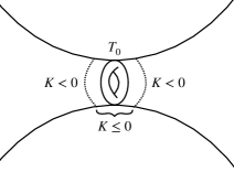
(a) No flat strips

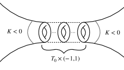
(b) With a flat strip

Figure 1.1. Type 1 manifolds

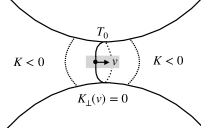
(a) No flat strips

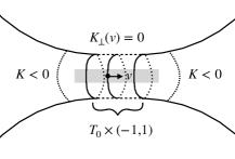
(b) With a flat strip

Figure 1.2. Type 2 surfaces

Pressure gap results:

Notice that when $M$ is type 1 or type 2, $\mathrm{Sing}$ is $T^{1}T_{0}$ or the unit tangent bundle of a (higher dimensional) flat strip containing $T_{0}$, i.e., $T^{1}\left(T_{0}\times\left(-1,1\right)\right)$; see Figure 1.1 and Figure 1.2 for examples. We are ready to state our first result on characterizing the pressure gap. We denote a radius $R$ tubular neighborhood of a set $S$ by $N_{R}(S)$.

Theorem A (Pressure gap criterion).

Let $M$ be a type 1 or type 2 manifold, and $\varphi:T^{1}M\to\mathbb{R}$ be a potential satisfying $\left.\varphi\right|_{\mathrm{Sing}}=C_{0}$ where $C_{0}$ is a constant. Suppose there exists $N_{R}(\mathrm{Sing})$ and constants $C,\varepsilon_{1},\varepsilon_{2}>0$ such that for $v\in N_{R}(\mathrm{Sing})$

(1.1) $$\varphi(v)-C_{0}\geq-C\left(|x_{v}|^{\frac{m}{2}+\varepsilon_{1}}+|\phi_{v}|^{\frac{m}{m+2}+\varepsilon_{2}}\right).$$

Then $P(\mathrm{Sing},\varphi)<P(\varphi)$.

Notice that via replacing $\varphi$ by $\varphi-C_{0}$, we may assume $\varphi|_{\mathrm{Sing}}=0$. We also remark that it is sufficient to have a lower bound of $\varphi-C_{0}$ near $\mathrm{Sing}$, since when $\varphi$ is much larger than $C_{0}$ it accumulates more pressure outside the singular set. In fact, we only need to exclude $\varphi$ that is very close to $C_{0}$ while it approaches $\mathrm{Sing}.$

Remark.

As mentioned in Example subsection, for the brevity and readability, we assume $M$ only contains only one flat torus $T_{0}$. Indeed, Theorem A holds given $\mathrm{Sing}$ is induced by finitely many codimension 1 totally geodesic flat subtori. Precisely, Theorem A is valid under the following assumptions:

1. $\mathrm{Sing}=\coprod_{i=0}^{k}T^{1}\mathsf{S}_{i}$, where $\mathsf{S}_{i}$ is a codimension 1 totally geodesic flat subtorus $T_{i}$ or a higher dimensional flat strip containing $T_{i}$.

2. $\varphi|_{T^{1}\mathsf{S}_{i}}=C_{i}$ is a constant for $i=0\cdots k$.

3. Without loss of generality, we assume $P(\varphi|_{T^{1}\mathsf{S}_{0}})=\max\{P(\varphi|_{T^{1}\mathsf{S}_{i}}):\ i=0\cdots k\}=P(\mathrm{Sing},\varphi)$. We only need $\varphi$ to satisfy (1.1) near $T^{1}\mathsf{S}_{0}$.

4. $M$ satisfies the curvature bounds near $\mathsf{S}_{0}$ as a type 1 or type 2 manifold.

Suppose $\mathrm{Sing}$ is induced by finitely many codimension 1 totally geodesic flat subtori. Then the result below in [BCFT18] follows the generalized version of Theorem A above.

Corollary (Locally constant potentials).

[BCFT18, Theorem B] If $\varphi$ is a locally constant function in a neighborhood of $\mathrm{Sing}$, then $P(\varphi)>P(\mathrm{Sing},\varphi)$.

Remark.

The biggest difference between [BCFT18] and our results is the shadowing orbit construction. [BCFT18] uses stable and unstable manifolds to build orbit segments that shadow orbit segments contained in the singular set. This approach works for all nonpositively curved manifolds, however, with less control. Our results require more delicate estimates on the shadowing orbits. To do this, we use bouncing orbits (see Figure 4.1) to shadow singular orbits, and the curvature bounds provide extra control over the shadowing orbits. See Section 3.1 for more discussions.

We call that a potential $\varphi$ has a phase transition at $q_{0}$ if the pressure map $q\mapsto P(q\varphi)$ fails to be differentiable at $q_{0}$. It is well-known that the uniqueness of equilibrium states implies the differentiability of the pressure map; see [Rue78].

Combining Theorem A and [BCFT18, Theorem A] we immediately get:

Theorem B (No phase transition).

Let $M$ and $\varphi$ be the same as in Theorem A. Suppose in addition that $\varphi$ is a Hölder continuous potential satisfying for $v\in N_{R}(\mathrm{Sing})$

(1.2) $$\left|\varphi(v)-C_{0}\right|\leq C\left(|x_{v}|^{\frac{m}{2}+\varepsilon_{1}}+|\phi_{v}|^{\frac{m}{m+2}+\varepsilon_{2}}\right).$$

Then $q\varphi$ has a unique equilibrium state for each $q\in\mathbb{R}$; thus, $\varphi$ has no phase transitions.

Remark.

The argument for Theorem B is still valid even if $\varphi$ is only controlled from below, i.e., satisfying (1.1). In a such case, the conclusion is that $q\varphi$ has a unique equilibrium state for $q>0$.

The proof of Theorem A follows an abstract pressure criterion (Proposition 7.2). For the readability, we postpone the details of this abstract result until Section 7. Roughly speaking, Proposition 7.2 shows that if the geodesic flow ${\mathcal{F}}$ possesses (1) “strong” specification property, (2) the singular set can be shadowed by nearby vectors, and if (3) the potential $\varphi$ decays fast enough, then $\varphi$ has a pressure gap.

Geometric potential results:

The second theme of this paper is contributed to studying behaviors of the geometric potential $\varphi^{u}:T^{1}M\to\mathbb{R}$ near $T_{0}$. Recall that $\varphi^{u}$ the geometric potential is defined as

$$\varphi^{u}(v):=-\lim_{t\to 0}\frac{1}{t}\log\det(df_{t}\mid_{E^{u}(v)})$$

where $E^{u}(v)$ is the unstable subspace (see Section 2 for details).

For type 2 surfaces without flat strips, Gerber-Niţică. [GN99, Theorem 3.1] and Gerber-Wilkinson [GW99, Lemma 3.3] gave Hölder continuity estimates for the geometric potential $\varphi^{u}$ near the $\mathrm{Sing}$. The following result shows that under a natural Ricci curvature constrain, similar Hölder continuity estimates can be extended to higher dimensional cases.

In what follows, we denote by $a(v)\approx b(v)$ near $S$, if there exists a neighborhood $N$ of $S$ and $C>1$ such that $C^{-1}b(v)\leq a(v)\leq Cb(v)$ for $v\in N$. We call $M$ has order $m$ Ricci curvature bounds, if the Ricci curvature ${\rm Ric}(v)$ vanishes uniformly to order $m-1$ on $T_{0}$; see (6.3).

Theorem C (Geometric potentials).

Let $M$ be a type 1 manifold without flat strips. Suppose $M$ has order $m$ Ricci curvature bounds, then near $\mathrm{Sing}$

$$-\varphi^{u}(v)\approx|x_{v}|^{\frac{m}{2}}+|\phi_{v}|^{\frac{m}{m+2}}.$$

Remark.

In general, normal curvature and the Ricci curvature have no strong relations. Only in the surface case, these two curvatures are the same. Nevertheless, we show, in the appendix, that if the Riemannian metric is a warped product, then Ricci curvature bounds and normal curvature bounds are equivalent.

In the majority of cases, the Hölder continuity of geometric potentials are unknown for nonuniformly hyperbolic systems, especially in higher dimension. As an immediate consequence of Theorem C, we have a partial result for higher dimensional manifolds:

Theorem D (Local Hölder continuity).

Under the same assumptions as Theorem C, the geometric potential $\varphi^{u}$ is Hölder continuous near $\mathrm{Sing}.$

On the other hand, as a consequence of Theorem C, we know that $\varphi^{u}$ is an edge case of the pressure gap criterion given in Theorem A (i.e., $\varepsilon_{1}=\varepsilon_{2}=0$). Moreover, it is known that manifolds (including surfaces) whose singular sets are unit tangent bundles of flat totally geodesic codimension 1 tori, the geometric potential $\varphi^{u}$ has a phase transition at $q=1$; see [BBFS21, P. 530] and [BCFT18, Theorem C].

In other words, Theorem C shows that the pressure gap criterion given in Theorem A is optimal, in the sense that there are examples on the boundary of our criterion which have no pressure gaps. (See Figure 1.3.)

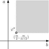
Figure 1.3. Region on which potentials $|\varphi(v)|\approx|x_{v}|^{a}+|\phi_{v}|^{b}$ have the pressure gap and no phase transitions.

In Figure 1.3 which describes the plane where each point on it corresponds to potentials $\varphi$ satisfying $-\varphi(v)\approx|x_{v}|^{a}+|\phi_{v}|^{b}$, the shaded region corresponds to potentials having the pressure gap and no phase transitions by Theorem A. The geometric potential $\varphi^{u}$ lies on the vertex $(\frac{m}{2},\frac{m}{m+2})$ of the shaded region.

We conclude this subsection by posting an open question:

Question.

Suppose $(a,b)$ lies on the boundary of the shaded region in Figure 1.3. Is there a potential $\varphi$ satisfying $|\varphi|\approx|x_{v}|^{a}+|\phi_{v}|^{b}$ near $\mathrm{Sing}$ such that $\varphi$ has a phase transition?

Examples:

The prototype of type 1 manifolds is the surface of revolution with profile $f(x)=1+|x|^{r}$, which is also the main example discussed in Lima-Matheus-Melbourne [LMM]. For higher dimension, one important example is the Heintze example (see Ballman-Brin-Eberlein [BBE85] or [BCFT18, Section 10.2].) The simplest version of the Heintze example is given by the following construction. One starts with a finite volume hyperbolic 3-manifold with one cusp, then removes the cusp and flattens the region near the cross-section. Recall that the cross-section of the cusp is a codimension 1 totally geodesic flat torus. We get the Heintze example by gluing two identical copies of the above 3-manifold along the cross-section; see Figure 1.1.

Type 2 surfaces (see Figure 1.2) were introduced in Gerber-Niţică [GN99] and Gerber-Wilkinson [GW99]. The archetype is a rank 1 nonpositive curved surface with an analytic metric. In such cases, it is a folklore result that $\mathrm{Sing}$ consists of unit tangent bundles of finitely many closed geodesics (see [BCFT18, Section 10.1] for a sketched proof).

We remark that for nonpositively curved surfaces Cao and Xavier [CX08] showed flat strips for nonpositively curved manifolds close up. However, in general we do not know if the singular geodesics or the (higher dimensional) zero curvature strips close up. Nevertheless, in all known examples, to the best of the authors knowledge, singular set all close up, and this leads to our hypothesis on the existence of $T_{0}$.

Historical remarks:

We remark that when the dynamical system is uniformly hyperbolic, there is no singular set. Hence, the pressure gap persists for nice a wide class of potentials and one can derive ergodic property for associated equilibrium states. The origin of this fact traces back to the work of Bowen [Bow74] for maps and Franco [Fra77] for flows. For nonuniformly hyperbolic systems, Climenhaga and Thompson [CT16] proposed to use the pressure gap as a condition to obtain ergodic properties of equilibrium states, especially, the uniqueness, as in the uniform hyperbolic cases.

[BCFT18] is the first work which analyzes the pressure gap condition in geometric contexts. They showed for closed rank 1 nonpositively curved manifolds, if $\varphi$ is locally constant near $\mathrm{Sing}$ then $\varphi$ has the pressure gap. It was inspired by Knieper’s work [Kni98] where the entropy gap $h_{{\rm top}}(\mathrm{Sing})<h_{{\rm top}}(\mathcal{F})$ was established as a consequence of the uniqueness of the measure of maximal entropy. Recall that the topological entropy $h_{{\rm top}}(\mathcal{F})$ is the pressure of the zero potential.

As in geometry, the Liouville measure is an equilibrium state for the geometric potential. Ergodic properties of equilibrium states have been studied extensively. There are several new contributions to this direction using the Climenhaga-Thompson strategy (see [CT21] for a survey for the strategy). For example, Chen, Kao, and Park [CKP20, CKP21] worked on no focal points setting; Climenhaga, Knieper, and War focused on no conjugate points manifolds [CKW21]; Call, Constantine, Erchenko, and Sawyer [CCE⁺] discussed flat surfaces with singularities.

There are many other relevant discussions on the ergodic properties of the equilibrium states. For instance, the uniqueness is also discussed in [GR19], the Kolmogorov property is studied in [CT22], the Bernoulli property is investigated in [Pes77, BG89, OW98, LLS16, CT22, ALP], and the central limit theorem is examined in [TW21, LMM].

For geometric potentials of rank 1 surfaces, Burns and Gelfert [BG14] pointed out the existence of the phase transition. This was also confirmed in [BCFT18] using a different approach. A recent work of Burns, Buzzi, Fisher, and Sawyer [BBFS21] further investigated the edge case of $\varphi=q\varphi^{u}$ for $q=1$. They showed that Liouville measure is the only equilibrium state not supported on $\mathrm{Sing}.$ However, the Hölder continuity of $\varphi^{u}$ is even less known. It is only assured by Gerber and Wilkinson [GW99, Theorem I] for type 2 surfaces. Much less is known about $\varphi^{u}$ in higher dimension cases.

Outline of paper:

In Section 2, we recall the relevant background materials from geometry and dynamics. In Section 3, we introduce the main shadowing technique and a key inequality for proving Theorem A. Section 4 and Section 5 are devoted to technical estimates in type 1 and type 2 settings by analyzing the relevant Riccati equations. Section 6 focuses on the geometric potential and the proof of Theorem C. The proof of Theorem A is presented in Section 7 as a consequence of a more general pressure gap criterion Proposition 7.2. In Appendix, we show that for warped product metrics normal curvature bounds and Ricci curvature bounds are equivalent.

Acknowledgments:

The authors are grateful to Amie Wilkinson for proposing this question, and to Keith Burns, Vaughn Climenhaga, Todd Fisher, and Dan Thompson for enlightening discussions. Lastly, the authors would like to dedicate this work to Todd Fisher for the inspirations that he brought to us in his too short but luminous life.

2. Preliminary

2.1. Geometry of nonpositively curved manifolds

In this subsection, we will survey relevant geometric features of nonpositively curved manifolds. More comprehensive survey of these results can be found in [Bal95, Ebe01].

Let $M$ be a closed nonpositively curved manifold, and $\{f_{t}\}_{t\in\mathbb{R}}$ the geodesic flow on the unit tangent bundle $T^{1}M$. The tangent bundle $TT^{1}M$ contains three $df_{t}$-invariant continuous bundles $E^{s},E^{u}$, and $E^{c}$. The bundle $E^{c}$ is one-dimensional along the flow direction, and the other two bundles $E^{s/u}$, which are orthogonal to $E^{c}$ with respect to the Sasaki metric, can be described via the use of Jacobi fields. If $M$ is negatively curved, then these three bundles form a splitting of $TT^{1}M$.

A Jacobi field $J$ along a geodesic $\gamma$ is a vector field along $\gamma$ satisfying the Jacobi equation

$$J^{\prime\prime}(t)+R(J(t),\gamma^{\prime}(t))\gamma^{\prime}(t)=0$$

where $R$ is a Riemannian curvature tensor. A Jacobi field $J$ is orthogonal if there exists $t_{0}\in\mathbb{R}$ such that $J(t_{0})$ and $J^{\prime}(t)$ are perpendicular to $\gamma^{\prime}(t_{0})$. It is well known that when this orthogonal property holds at some $t_{0}\in\mathbb{R}$, then it holds for all $t\in\mathbb{R}$. A Jacobi field $J$ is parallel if $J^{\prime}(t)=0$ for all $t\in\mathbb{R}$.

Denoting the space of orthogonal Jacobi fields along $\gamma$ by $\mathcal{J}^{\perp}(\gamma)$, we can identify $T_{v}T^{1}M$ with $\mathcal{J}^{\perp}(\gamma_{v})$ as follows. Consider a vector $v\in T_{p}M$. Using the Levi-Civita connection the tangent space $T_{v}TM$ at $v$ may be identified with the direct sum $H_{v}\oplus V_{v}$ of horizontal and vertical subspace, respectively, each isomorphic to $T_{p}M$ equipped with the norm induced from the Riemannian metric on $M$. The Sasaki metric on $TM$ is defined by declaring $H_{v}$ and $V_{v}$ to be orthogonal. Restricted to $T^{1}M$, the tangent space $T_{v}T^{1}M$ corresponds to $H_{v}\oplus v^{\perp}$ under this identification. Then any vector $\xi\in T_{v}T^{1}M$ for $v\in T^{1}M$ may be written as $(\xi_{h},\xi_{v})$ and can be identified with an orthogonal Jacobi field $J_{\xi}\in\mathcal{J}^{\perp}(\gamma_{v})$ along $\gamma_{v}$ with the initial conditions $(J_{\xi}(0),J^{\prime}_{\xi}(0))=(\xi_{h},\xi_{v})$. Moreover, the Sasaki norm of $df_{t}(\xi)$ satisfies

$$\|df_{t}(\xi)\|^{2}=\|J_{\xi}(t)\|^{2}+\|J^{\prime}_{\xi}(t)\|^{2}.$$

The stable subspace $E^{s}(v)$ at $v\in T^{1}M$ is then defined as

$$E^{s}(v):=\{\xi\in T_{v}T^{1}M\colon\|J_{\xi}(t)\|\text{ is bounded for }t\geq 0\}.$$

Similarly, the unstable subspace $E^{u}(v)$ consists of vectors $\xi\in T_{v}T^{1}M$ where $\|J_{\xi}(t)\|$ is bounded for $t\leq 0$. Notice that the subbundles $E^{u}(v)$ and $E^{s}(v)$ are integrable to the respective foliations $W^{u}(v)\subset T^{1}M$ and $W^{s}(v)\subset T^{1}M$. The footprints of $W^{u}(v)$ and $W^{s}(v)$ on $M$ are called the unstable and stable horospheres, which are denoted by $H^{u}(v)$ and $H^{s}(v)$, respectively.

The rank of a vector $v\in T^{1}M$ is the dimension of the space of parallel Jacobi fields along $\gamma_{v}$, which coincides with the number $1+\dim(E^{s}\cap E^{u})$. We say the manifold is rank 1 if it has at least one rank 1 vector. We will focus mainly on closed rank 1 nonpositively curved manifolds in this paper.

The singular set is a set of vectors on which the geodesic flow fails to display uniform hyperbolicity and it is defined by

$$\mathrm{Sing}:=\{v\in T^{1}M\colon E^{s}(v)\cap E^{u}(v)\neq 0\}.$$

The singular set is closed and $\mathcal{F}$-invariant, and in the case where $M$ is a surface the singular set can be characterized as the set of vectors $v$ where the Gaussian curvature $K(\gamma_{v}(t))$ vanishes for all $t\in\mathbb{R}$. The complement of the singular set is the regular set

$$\mathrm{Reg}:=T^{1}M\setminus\mathrm{Sing}.$$

The geodesic flow restricted to the regular set is hyperbolic, but the degree of hyperbolicity, which can be measured by the function

$$\lambda(v):=\min(\lambda^{u}(v),\lambda^{s}(v))$$

where $\lambda^{u}(v)$ is the minimum eigenvalue of the shape operator on the unstable horosphere $H^{u}(v)$ at $v$. Using $\lambda$ we can define nested compact subsets $\{\mathrm{Reg}(\eta)\}_{\eta>0}$ of $\mathrm{Reg}$ where

$$\mathrm{Reg}(\eta):=\{v\in\mathrm{Reg}\colon\lambda(v)\geq\eta\}.$$

These subsets may be viewed as uniformity blocks in the sense of Pesin theory, where the hyperbolicity is uniform. More details and properties of the function $\lambda$ can be found in [BCFT18].

The geometric potential $\varphi^{u}:T^{1}M\to\mathbb{R}$ is an important potential that measures the infinitesimal volume growth in the unstable direction:

$$\varphi^{u}(v):=-\lim_{t\to 0}\frac{1}{t}\log\det(df_{t}\mid_{E^{u}(v)})=-\frac{d}{dt}\Big{|}_{t=0}\log\det(df_{t}\mid_{E^{u}(v)}).$$

To study the geometric potential, it is convenient to study Riccati equations. Interestingly, the shape operator of unstable (and unstable) horosphere is a solution of a Riccati equation. To see this, we start from introducing terminologies.

Let $H\subset M$ be a hypersurface orthogonal to $\gamma_{v}$ at $\pi v$ where $\pi:T^{1}M\to M$ is the canonical projection. An orthogonal Jacobi field $J\in\mathcal{J}^{\perp}(\gamma_{v})$ is called a $H$-Jacobi field along $\gamma_{v}$, if $J$ comes from varying $\gamma_{v}$ through unit speed geodesics orthogonal to $H$. We denote the set of $H$- Jacobi fields by $\mathcal{J}_{H}(\gamma_{v})$ . The shape operator on $H$ is the symmetric linear operator $U:T_{\pi v}H\to T_{\pi v}H$ defined by $U(v)=\nabla_{v}N$, where $N$ is the unit normal vector field toward the same side as $v$.

We are particularly interested in the unstable horosphere $H=H^{u}(v)$ at $v$. In this case, $J_{H^{u}}(\gamma_{v})$ coincides with the space of unstable Jacobi field $J^{u}(\gamma_{v})$. For $t\in\mathbb{R}$, let $U_{v}^{u}(t):T_{\pi v}H^{u}(f_{t}v)\to T_{\pi v}H^{u}(f_{t}v)$ be the shape operator of the unstable horosphere $H^{u}(f_{t}v)$. We know $U_{v}^{u}(t)$ is a a positive semidefinite symmetric linear operator on $(f_{t}v)^{\perp}$, and for any unstable Jacobi field $J(t)$ it satisfies $J^{\prime}(t)=U_{v}^{u}(t)J(t)$; see [BCFT18, Lemma 2.9].

For any vector $v\in T^{1}M$, let $\mathcal{K}(v):v^{\perp}\to v^{\perp}$ is the symmetric linear map defined via $\langle\mathcal{K}(v)X,Y\rangle:=\langle R(X,v)v,Y\rangle$ for $X,Y\in v^{\perp}$. Using the Jacobi equation, for an unstable Jacobi field $J(t)$ we know $J^{\prime\prime}(t)+K(f_{t}v)J(t)=0$ and $J^{\prime}(t)=U_{v}^{u}(t)J(t)$. Thus we get the operator-valued Riccati equation:

(2.1) $$U_{v}^{u}(t)+\left(U_{v}^{u}(t)\right)^{2}+{\mathcal{K}}(\dot{\gamma}_{v}(t))=0;$$

see [BCFT18, (7.6)]. Using the above notation, the Ricci curvature ${\rm Ric}(v)$ at $v$ is defined as the trace of the map ${\mathcal{K}}(v)$.

2.2. Thermodynamic formalism

We now briefly survey relevant results in thermodynamic formalism. The general notion of topological entropy and pressure described below can be defined for an arbitrary flow $\mathcal{F}=\{f_{t}\}_{t\in\mathbb{R}}$ on a compact metric space $(X,d)$.

For any $t>0$, we define a new metric $d_{t}$ on $X$ where

$$d_{t}(x,y):=\max\limits_{0\leq\tau\leq t}d(f_{t}x,f_{t}y),$$

and the corresponding $\delta$-ball around $x\in X$ in $d_{t}$-metric will be denoted by $B_{t}(x,\delta)$. We say a subset $E$ of $X$ is $(t,\delta)$-separated if $d_{t}(x,y)\geq\delta$ for distinct $x,y\in E$. Moreover, we will identify $(x,t)\in X\times[0,\mathbb{R}^{+})$ with the orbit segment of length $t$ starting at $x$.

Let $\varphi\colon X\to\mathbb{R}$ be a continuous function on $X$, which we often call a potential. We define ${\displaystyle\Phi(x,t):=\int_{0}^{t}\varphi(f_{\tau}x)\,d\tau}$ to be the integral of $\varphi$ along an orbit segment $(x,t)$. For any subset $\mathcal{C}\in X\times[0,\mathbb{R}^{+})$, we let $\mathcal{C}_{t}$ be the subset of $\mathcal{C}$ consisting of orbit segments of length $t$. We define

$$\Lambda(\mathcal{C},\varphi,\delta,t)=\sup\Big{\{}\sum\limits_{x\in E}e^{\Phi(x,t)}\colon E\subset\mathcal{C}_{t}\text{ is }(t,\delta)-\text{separated}\Big{\}}.$$

The topological pressure of $\varphi$ on $\mathcal{C}$ is then defined by

$$P(\mathcal{C},\varphi):=\lim\limits_{\delta\to 0}\limsup\limits_{t\to\infty}\frac{1}{t}\log\Lambda(\mathcal{C},\varphi,\delta,t).$$

When $\mathcal{C}$ is the entire orbit space $X\times[0,\mathbb{R}^{+})$, then we denote it by $P(\varphi)$ and call it the topological pressure of $\varphi$. In the case where $\varphi\equiv 0$, the resulting pressure $P(0)$ is called the topological entropy of the flow $\mathcal{F}$ denoted by $h_{top}(\mathcal{F})$.

Denoting by $\mathcal{M}(\mathcal{F})$ the set of all $\mathcal{F}$-invariant measures on $X$, the pressure $P(\varphi)$ satisfies the variational principle

$$P(\varphi)=\sup\limits_{\mu\in\mathcal{M}(\mathcal{F})}\Big{\{}h_{\mu}(\mathcal{F})+\int\varphi\,d\mu\Big{\}}$$

where $h_{\mu}(\mathcal{F})$ is the measure-theoretic entropy of $\mu$. Any invariant measure $\mu\in\mathcal{M}(\mathcal{F})$ attaining the supremum is called an equilibrium state for $\varphi$. Likewise, any invariant measure attaining the supremum when $\varphi\equiv 0$ is called a measure of maximal entropy.

2.3. Codimension 1 totally geodesic flat torus and Fermi coordinates

Let $M$ be an $n$-dimensional closed rank 1 nonpositively curved manifold and $T_{0}$ a totally geodesic $(n-1)$-torus in $M$ with $K\equiv 0$ on any $x\in T_{0}$. We further suppose that the complement of $T_{0}$ is negatively curved and that curvature away from a small tubular neighborhood of $T_{0}$ admits a uniform upper bound strictly smaller than 0. A more precise control on the curvature on the tubular neighborhood will be specified later depending on the setting under consideration.

In what follows, we fix a fundamental domain in $\widetilde{M}$ the universal covering of $M$ and (abusing the notation) continue denoting the lifts of $p\in M$ and $v\in T_{p}M$ by $p$ and $v$, respectively. Recall that the Fermi coordinate of $p$ is given by $(s,x)$ where $s$ is an $(n-1)$-dimensional coordinate on $\widetilde{T}_{0}$ and $x$ measures the signed distance on $\widetilde{M}$ to $\widetilde{T}_{0}$.

For $p\in\widetilde{M}$ near $\widetilde{T}_{0}$, by $x(p)$ we mean the $x$-coordinate of $p$. For any $v\in T_{p}\widetilde{M}$ with $p$ near $\widetilde{T}_{0}$, we define $x_{v}:=x(p)$ and denote by $\phi_{v}$ the signed angle between $v$ and the hypersurface $x=x(p)$; we adopt the convention that $\phi_{v}=\pi/2$ when $v=\partial/\partial x$. We also define

(2.2) $$x_{v}(\tau):=x(\gamma_{v}(\tau))\text{ and }\phi_{v}(\tau):=\phi(\gamma_{v}^{\prime}(\tau)).$$

When there is no confusion, we may write $x_{v}$ and $\phi_{v}$ for $x_{v}(0)$ and $\phi_{v}(0)$, respectively.

Remark 2.1.

With respect to Fermi coordinates $(s,x)$, the curve $s=\text{const.}$ is always a geodesic perpendicular to $\widetilde{T}_{0}$, while $(s(t),x(t))$ with $x(t)\equiv x_{0}$ for some $x_{0}$ is not a geodesic unless $x_{0}=0$ and $s(t)$ is linear.

For $\varepsilon>0$ small, the Riemannian metric near $\widetilde{T}_{0}$ can be written as

(2.3) $$g=dx^{2}+g_{x},\quad|x|\leq\varepsilon$$

where $g_{x}$ is the Riemannian metric on $\widetilde{T}_{x}:=\widetilde{T}_{0}\times\{x\}$. In particular, $g_{0}$ is the Euclidean metric on $\widetilde{T}_{0}$.

Denoting by $X:=\partial/\partial x$ the vertical vector field, the second fundamental form on $\widetilde{T}_{x}$ is defined via

$$\text{II}(v,w):=\langle\nabla_{v}X,w\rangle,$$

for any $v,w\in T_{(s,x)}\widetilde{T}_{x}$. The shape operator $U(s,x):T_{(s,x)}\widetilde{T}_{x}\to T_{(s,x)}\widetilde{T}_{x}$ is defined via

$$\text{II}(v,w)=\langle U(s,x)v,w\rangle.$$

As II is bilinear and symmetric, the shape operator $U(s,x)$ is diagonalizable. Its eigenvalues

$$\lambda_{1}(s,x)\leq\lambda_{2}(s,x)\leq\cdots\leq\lambda_{n-1}(s,x)$$

are called principal curvatures at $(s,x)$.

For any geodesic $\gamma(t)=(s(t),x(t))$ near $\widetilde{T}_{0}$, by the first variation formula we have

(2.4) $$x^{\prime}=\sin\phi,$$

where $\phi(t):=\phi(\gamma^{\prime}(t))$, which then gives $x^{\prime\prime}=\phi^{\prime}\cos\phi$.

We denote by

$$\gamma^{\prime}_{\perp}(t):=\gamma^{\prime}(t)-\langle\gamma^{\prime}(t),X\rangle X$$

the component of $\gamma^{\prime}(t)$ that is orthogonal to $X$. Then $|\gamma^{\prime}_{\perp}|=\cos\phi$.

Lemma 2.2.

If $\gamma(t)=(s(t),x(t))$ is a geodesic on $\widetilde{M}$ near $\widetilde{T}_{0}$, we have

$$x^{\prime\prime}=\text{II}(\gamma^{\prime}_{\perp},\gamma^{\prime}_{\perp})\in[\lambda_{1}(s,x)\cos^{2}\phi,\lambda_{n-1}(s,x)\cos^{2}\phi].$$

Proof.

By (2.4), we have $x^{\prime}=\sin\phi=\langle X,\gamma^{\prime}(t)\rangle$. Thus

$$x^{\prime\prime}=\frac{d}{dt}\langle X,\gamma^{\prime}(t)\rangle=\langle\nabla_{\gamma^{\prime}(t)}X,\gamma^{\prime}(t)\rangle=\langle\nabla_{\gamma^{\prime}_{\perp}(t)}X,\gamma^{\prime}_{\perp}(t)\rangle=\text{II}(\gamma^{\prime}_{\perp},\gamma^{\prime}_{\perp}).$$

Note that the third equality uses the fact $\nabla_{X}X=0$; see Remark 2.1. Since $|\gamma^{\prime}_{\perp}|=\cos\phi$, we have

$$\text{II}(\gamma^{\prime}_{\perp},\gamma^{\prime}_{\perp})\geq\lambda_{1}(s,x)|\gamma^{\prime}_{\perp}|^{2}=\lambda_{1}(s,x)\cos^{2}\phi$$

and

$$\text{II}(\gamma^{\prime}_{\perp},\gamma^{\prime}_{\perp})\leq\lambda_{n-1}(s,x)\cos^{2}\phi.$$

This completes the proof. ∎

Remark 2.3.

When $M$ is a surface, then $T_{0}$ is a closed geodesic. In this case the Riemannian metric (2.3) near $\widetilde{T}_{0}$ may be written as

(2.5) $$g=dx^{2}+G(s,x)^{2}ds^{2}$$

with $G(s,0)\equiv 1$. The Gaussian curvature is given by $K=-G_{xx}/G$, and the second fundamental form at $\widetilde{T}_{x}$ is $G_{x}/G$. In particular, by Lemma 2.2, $x^{\prime\prime}$ admits the following expression

(2.6) $$x^{\prime\prime}=\lambda(s,x)\cos^{2}\phi=\frac{G_{x}}{G}\cos^{2}\phi.$$

3. Preparation and outline for pressure gaps results

3.1. Shadowing map

To distinguish vectors in $\mathrm{Sing}$ and generic vectors in $T^{1}M$, we will use different fonts to denote them, more precisely, we will write $\mathsf{v}\in\mathrm{Sing}$ and $v\in T^{1}M$. Given an orbit segment $(\mathsf{v},t)\in T^{1}M\times\mathbb{R}^{+}$ with $\mathsf{v}\in\mathrm{Sing}$, we now describe a method for constructing a new orbit segment that shadows $(\mathsf{v},t)$. Though simple, this construction will be crucial in proving Theorem A and Theorem D.

For any $\mathsf{v}\in\text{Sing}$, suppose $\pi(\tilde{\mathsf{v}})=(s_{0},0)$ for some $s_{0}$. For any $t>0$ and any $R>0$ such that the Fermi coordinates $(s,x)$ are well-defined for $|x|<R$, there exists $s_{1}\in\mathbb{R}$ such that the distance on $\widetilde{M}$ between $(s_{0},R)$ and $(\pi(\tilde{f}_{s_{1}}\tilde{\mathsf{v}}),R)$ is equal to $t$; see Figure 3.1. Denoting by $\tilde{\gamma}$ the geodesic connecting these two points and by $\gamma$ the corresponding geodesic in $M$, we define

(3.1) $$\Pi_{t,R}(\mathsf{v}):=\gamma^{\prime}(0).$$

Throughout the paper, we will often write $w_{\mathsf{v}}$, or simply $w$, to denote $\Pi_{t,R}(\mathsf{v})$ whenever the context is clear.

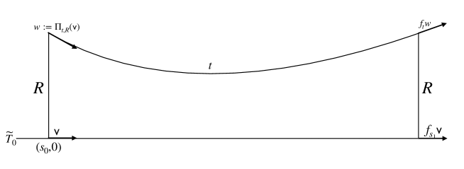
Figure 3.1. Construction of $\Pi_{t,R}$

The next few lemmas establish a few properties on the map $\Pi_{t,R}$.

Lemma 3.1.

For any $\mathsf{v}\in\mathrm{Sing}$ and $t>0$, the following statements hold:

1. For any $R>0$, the function $x_{w}(\tau)$ is convex for any $\tau\in[0,t]$.

2. There exists $R_{0}>0$ such that for any $R\in(0,R_{0})$,

   $$|\phi_{w}(\tau)|<\frac{\pi}{4}$$

   for all $\tau\in[0,t]$.

3. For any $R>0$, there exists $\eta=\eta(R)>0$ such that $w,f_{t}w\in\text{Reg}(\eta)$.

Proof.

For (1), it is not hard to see from the construction of $\Pi_{t,R}$ that $|\phi_{w}(\tau)|\leq\pi/2$ and $\phi_{w}^{\prime}(\tau)\geq 0$ for all $\tau\in[0,t]$. The statement then is a consequence of $x_{w}^{\prime\prime}(\tau)=\phi_{w}^{\prime}(\tau)\cos\phi_{w}(\tau)$ from (2.4).

For (2), it is clear that

$$|\phi_{w}(\tau)|\leq\max\{|\phi_{w}(0)|,|\phi_{w}(t)|\}$$

for all $\tau\in[0,t]$. We then observe that $|\phi_{w}(0)|\leq|\phi(\gamma^{\prime}_{w,s}(0))|$ where $\gamma_{w,s}$ is the geodesic with the same initial point as $\gamma_{w}$ that is forward asymptotic to $\widetilde{T}_{0}$. The statement then follows as the function

$$R\mapsto\sup\{|\phi(u)|\colon u\in W^{s}(\mathsf{v})\text{ for some }\mathsf{v}\in\mathrm{Sing}\text{ and }x(\pi u)=R\}$$

vanishes when $R=0$ and varies continuously in $R$. By repeating the same argument with the unstable manifolds $W^{u}(\mathsf{v})$ for $\mathsf{v}\in\mathrm{Sing}$, we can find $R_{0}>0$ with the desired property.

For (3), any unit vector $v\in T^{1}M$ whose lift $\tilde{v}\in T^{1}\widetilde{M}$ satisfies $x(\pi(\tilde{v}))\neq 0$ belongs to $\mathrm{Reg}$. Since $\mathrm{Reg}$ is exhausted by compact subsets $\mathrm{Reg}(\eta)$ and the flat torus $T_{0}$ in $M$ is compact, the statement follows. ∎

Lemma 3.2.

There exists $R_{1}>0$ such that for any $R\in[0,R_{1}]$, $t\gg 0$, $\delta>0$ sufficiently small, and a $(t,\delta)$-separated subset $E_{t,\delta}$ of $\mathrm{Sing}$, the its lift $\Pi_{t,R}(E_{t,\delta})$ is a $(t,\delta/4)$-separated subset in $T^{1}M$.

Proof.

Let $\tilde{d}$ be the Riemannian metric on $\widetilde{M}$ by lifting $d$, and $\tilde{d}_{t}$ be the lift of $d_{t}$. For any $R>0$ and $x\in\widetilde{T}_{0}$, let $x_{R}\in\widetilde{M}$ be the point corresponding to $(x,R)$ in the Fermi coordinates. We can choose $R_{1}>0$ such that for any $R\in[0,R_{1}]$ and any distinct $x,y\in\widetilde{M}$, we have

(3.2) $$\frac{\tilde{d}(x_{R},y_{R})}{\tilde{d}(x,y)}\in\Big{[}\frac{1}{2},2\Big{]}.$$

For any $\mathsf{v}_{1},\mathsf{v}_{2}\in\mathrm{Sing}$, $R\in[0,R_{1}]$, and $t\gg 0$, consider $w_{i}:=\Pi_{t,R}(\mathsf{v}_{i})$. Suppose $d_{t}(w_{1},w_{2})\leq\delta/4$. The lemma would follow once we establish $d_{t}(\mathsf{v}_{1},\mathsf{v}_{2})\leq\delta$.

First we have $\tilde{d}_{t}(\tilde{w}_{1},\tilde{w}_{2})\leq\delta/4$. We define two convex functions $\rho_{1}(\tau)$ and $\rho_{2}(\tau)$ for $\tau\in[0,t+1]$ as

$$\rho_{1}(\tau)=\tilde{d}(\gamma_{\tilde{\mathsf{v}}_{1}}(\tau),\gamma_{\tilde{\mathsf{v}}_{2}}(\tau))\text{ and }\rho_{2}(\tau)=\tilde{d}(\gamma_{\tilde{w}_{1}}(\tau),\gamma_{\tilde{w}_{2}}(\tau)).$$

From the definition of the metric $d_{t}$, the inequality $\tilde{d}_{t}(\tilde{w}_{1},\tilde{w}_{2})\leq\delta/4$ translates to $\rho_{2}(\tau)\leq\delta/4$ for all $\tau\in[0,t+1]$.

Since $(\gamma_{\tilde{\mathsf{v}}_{i}}(\tau),R)$ is equal to $\gamma_{\tilde{w}_{i}}(\tau)$ at $\tau=0$ and $\tau=t$, unless $\rho_{1}=0$ it follows from (3.2) that the ratio $\rho_{2}/\rho_{1}$ belongs in the range $[\frac{1}{2},2]$ at $\tau=0$ and $\tau=t$. From the convexity $\rho_{1}$ attains its maximum at an endpoint, and hence it is enough to show $\max(\rho_{1}(0),\rho_{1}(t+1))\leq\delta$ in order to conclude that $d_{t}(\mathsf{v}_{1},\mathsf{v}_{2})\leq\tilde{d}_{t}(\tilde{\mathsf{v}}_{1},\tilde{\mathsf{v}}_{2})\leq\delta$.

If $\rho_{1}(0)=0$, then $\rho_{1}(t)$ is necessarily non-zero, and applying (3.2) at $\tau=t$ gives $\rho_{1}(t)\leq\delta/2$. As geodesics in $\widetilde{T}_{0}$ are straight lines, $\rho_{1}$ is a linear function. Since $t\gg 0$, we then have $\rho_{1}(t+1)\leq\delta$ as required. If $\rho_{1}(t)=0$ instead, similar argument would show that $\rho_{1}(0)\leq\delta/2$ and $\rho_{1}(t+1)\leq\delta$.

In the case where neither $\rho_{1}(0)$ nor $\rho_{1}(t)$ is zero, we have $\rho_{1}(0)\leq\delta/2$ and $\rho_{1}(t)\leq\delta/2$ by (3.2). Again using the fact that $t\gg 0$ and geodesics in $\widetilde{T}_{0}$ are straight lines, we deduce $\rho_{1}(t+1)\leq\delta$ as required. ∎

Remark 3.3.

From here on, we will assume that $R$ belongs to $[0,\min(R_{0},R_{1})]$ with $R_{0},R_{1}$ defined as in above lemmas. In particular, we will often evoke Lemma 3.1 to use the inequality

$$\cos\phi_{w}(\tau)\leq\Big{[}\frac{\sqrt{2}}{2},1\Big{]}$$

for any $w=\Pi_{t,R}(\mathsf{v})$ and $\tau\in[0,t]$. Lemma 3.2 will mainly be used in establishing the pressure gap in Section 7.

3.2. Key inequality and the outline of Theorem A

In this subsection, we provide a brief outline of what consist of the remaining sections. Recall from Lemma 3.1 that $x_{w}(\tau)$ is a convex function on $\tau\in[0,t]$ for any $w=\Pi_{t,R}(\mathsf{v})$, and hence there exists a well-defined number $\tilde{t}\in[0,t]$ such that

(3.3) $$x_{w}(\tilde{t})=\min_{\tau\in[0,t]}x_{w}(\tau)$$

and that $\tilde{t}$ is the smallest among all such numbers. In the case where $x_{w}(\tau)$ is strictly convex, there is a unique $\tilde{t}$ which attains the minimum of $x_{w}(\tau)$. Notice that $x^{\prime}_{w}(\tau)\leq 0$ and $\phi_{w}(\tau)\leq 0$ for $\tau\in[0,\tilde{t}\,]$.

The goal of the next few sections is to establish bounds on the distance $x_{w}(\tau)$ and the angle $\phi_{w}(\tau)$ under the assumption that the normal curvature $K_{\perp}$ vanishes to the order of $m-1$ at $T_{0}$ and that the curvature near $T_{0}$ is controlled; see Section 4 and 5 for the precise description of the setting. In particular, we will show that for suitable $R>0$, there exists $Q=Q(R)>1$ independent of $t$ such that the shadowing vector $w=\Pi_{t,R}(\mathsf{v})$ for any $\mathsf{v}\in\mathrm{Sing}$ and any $t>0$ satisfies

(3.4) $$\begin{split}Q^{-1}(\tau+1)^{-\frac{2}{m}}\leq&x_{w}(\tau)\leq Q(\tau+1)^{-\frac{2}{m}},\\ &|\phi_{w}(\tau)|\leq Q[(\tau+1)^{-\frac{m+2}{m}}-(\tilde{t}+1)^{-\frac{m+2}{m}}]\end{split}$$

for any $\tau\in[0,\tilde{t}\,]$. From its derivation in Proposition 4.2 and 5.3, it will be clear that analogous inequality holds for $\tau\in[\tilde{t},t]$ by simply applying the symmetric argument starting from $\tau=t$ instead of $\tau=0$:

(3.5) $$\begin{split}Q^{-1}(t-\tau+1)^{-\frac{2}{m}}\leq&x_{w}(\tau)\leq Q(t-\tau+1)^{-\frac{2}{m}},\\ &|\phi_{w}(\tau)|\leq Q[(t-\tau+1)^{-\frac{m+2}{m}}-(\tilde{t}+1)^{-\frac{m+2}{m}}].\end{split}$$

In the setting considered in Section 4 where a uniform control on the curvature $K_{\perp}$ is assumed on the entire $\widetilde{T}_{0}$, the angle $|\phi_{w}(\tau)|$ from (3.4) and (3.5) admits the corresponding lower bound also; see Proposition 4.2.

These estimates, once established, are particularly useful when considered with potentials $\varphi$ satisfying (1.1) near $\mathrm{Sing}$ (with $C_{0}=0$):

$$\varphi(v)\geq-C\left(|x_{v}|^{\frac{m}{2}+\varepsilon_{1}}+|\phi_{v}|^{\frac{m}{m+2}+\varepsilon_{2}}\right)$$

for some $\varepsilon_{1},\varepsilon_{2},C>0$. In the setting considered by Gerber and Wilkinson [GW99] where $M$ is a surface (see Section 5 for details) fits in with the assumption on $K_{\perp}$ described in the above paragraph, and $\varphi$ satisfying (1.1) is related to the geometric potential as elaborated more in the next subsection.

Assuming the estimates (3.4) and (3.5), we now derive useful consequences from them when considered with potentials $\varphi$ satisfying (1.1). We will see in Section 7 that, along with certain properties of the geodesic flow, these results serve as sufficient criteria for the potential $\varphi$ to have the pressure gap. From direct integration using the estimates (3.4) and (3.5) we immediately get

Proposition 3.4.

For some $R>0$, suppose that the shadowing vector $w=\Pi_{t,R}(\mathsf{v})$ satisfies (3.4) and (3.5) and that there exist $\varepsilon_{1},\varepsilon_{2},C>0$ such that the potential $\varphi$ satisfies

$$\varphi(v)\geq-C\left(|x_{v}|^{\frac{m}{2}+\varepsilon_{1}}+|\phi_{v}|^{\frac{m}{m+2}+\varepsilon_{2}}\right)$$

near $\mathrm{Sing}$. Then there exists $Q=Q(R,C,\varepsilon_{1},\varepsilon_{2})>0$ such that for any $t>0$ and $\mathsf{v}\in\text{Sing}$, we have

$$\int_{0}^{t}\varphi(f_{\tau}w_{\mathsf{v}})d\tau\geq-Q.$$

Corollary 3.5 (Key inequality).

Under the assumptions of Proposition 3.4, for any sufficiently small $\delta>0$, there exists $Q>0$ independent of $t$ such that

$$\int_{0}^{t}\varphi(f_{\tau}u)d\tau\geq-Q$$

for any $u\in B_{t}(w,\delta)$ where $w=\Pi_{t,R}(\mathsf{v})$ for some $\mathsf{v}\in\mathrm{Sing}$.

Proof.

We begin by intersecting the geodesic $\gamma_{u}(\tau)$ with the hyperplane $x=R$ so that there are exactly two intersection points, each near $\pi(u)$ and $\pi(f_{t}u)$; see Figure 3.2. We denote by $(u_{0},t_{0})$ the orbit segment connecting such intersection points. Since two orbit segments $(u,t)$ and $(u_{0},t_{0})$ differ only at either ends by length at most $2\delta$, there exists a constant $C_{\delta}$ depending only on $\delta$ and $\|\varphi\|$ such that

$$\Big{|}\int_{0}^{t}\varphi(f_{\tau}u)d\tau-\int_{0}^{t_{0}}\varphi(f_{\tau}u_{0})d\tau\Big{|}<C_{\delta}.$$

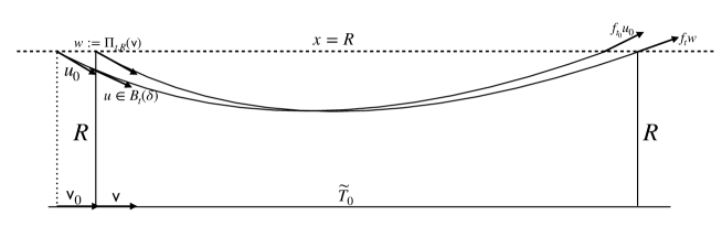
Figure 3.2. Figure for Corollary 3.5

Notice from its construction that $u_{0}$ is equal to $\Pi_{t_{0},R}(v_{0})$ for some $v_{0}\in\mathrm{Sing}$ near $v$, and hence, the integral ${\displaystyle\int_{0}^{t_{0}}\varphi(f_{\tau}u_{0})d\tau}$ admits a uniform lower bound independent of $t_{0}$ from the above proposition. Therefore, the same is true for ${\displaystyle\int_{0}^{t}\varphi(f_{\tau}u)d\tau}$ for $u\in B_{t}(w,\delta)$. ∎

4. Estimates for type 1 manifolds

Recalling that $X=\partial/\partial x$ is the vertical vector field, for any $v\in T\widetilde{M}$ that is not collinear with $X$ we define the normal curvature of $v$ by

(4.1) $$K_{\perp}(v):=K_{\sigma},\quad\sigma:=\text{span}\{v,X\}.$$

In this section, we will consider the first of the two settings which assumes that $K_{\perp}$ vanishes uniformly to order $m-1$. Namely, if $(s,x)$ are the Fermi coordinates along $\widetilde{T}_{0}$, there exists $C_{1},C_{2},\varepsilon>0$ such that

(4.2) $$-C_{1}|x(v)|^{m}\leq K_{\perp}(v)\leq-C_{2}|x(v)|^{m}$$

for any $v\perp X$ with $|x(v)|<\varepsilon$.

As outlined in Subsection 3.2, the main goal of this section is to prove that under the above assumption on $K_{\perp}$, the shadowing vector $w=\Pi_{t,R}(\mathsf{v})$ for any $\mathsf{v}\in\mathrm{Sing}$ satisfies the estimates on $x_{w}$ and $\phi_{w}$ claimed in (3.4).

Indeed, in this subsection we will derive estimates on $x_{v}(t)$ for generic vectors $v\in T^{1}M$ near $\tilde{T}_{0}$; namely, bouncing, asymptotic, and crossing vectors (see Definition 4.1). In Section 6, we will discuss behaviors of geometric potentials $\varphi^{u}$ with respect to bouncing, asymptotic and crossing vectors. Notice that by Definition 4.1, shadowing vectors $w=\Pi_{t,R}(\mathsf{v})$ are bouncing vectors.

Let $N_{R}(\widetilde{T}_{0}):=\left\{(s,x):s\in\widetilde{T}_{0}\ |x|<R\right\}$ be a tubular neighborhood of $\widetilde{T}_{0}$, $v\in T^{1}M$ and $\gamma_{v}(t)=(s_{v}(t),x_{v}(t))$ in the Fermi coordinates.

Definition 4.1.

Suppose $v\in T^{1}M$ such that $\gamma_{v}(0)\in N_{R}(\tilde{T}_{0})$. Let $-T_{1}=\inf\{t:\ \gamma_{v}(t)\in N_{R}(\widetilde{T}_{0})\}$ and $T_{2}=\sup\{t:\ \gamma_{v}(t)\in N_{R}(\widetilde{T}_{0})\}$. We say that $v$ (relative to $N_{R}(\widetilde{T}_{0})$) is

1. bouncing if $T_{1},T_{2}<\infty$ and $x_{v}(t)>0$ for $t\in(-T_{1},T_{2})$,

2. asymptotic if $T_{1}=\infty$ or $T_{2}=\infty$,

3. crossing if $T_{1},T_{2}<\infty$ and $x_{v}(t_{0})=0$ for $t_{0}\in(-T_{1},T_{2})$.

Please see Fig 4.1 for examples of these vectors. The definition and the study of these vectors are inspired by [LMM]. Notice that according to Lemma 5.5 the above definition is well-defined when $R$ is sufficiently small. Moreover, by definition all shadowing vectors are bouncing vectors and asymptotic vectors are limiting cases of the bouncing vectors. More precisely, one can regard asymptotic vectors as bouncing vectors $v$ with the minimal of $x_{v}$ (when $\phi(v)<0$) occurring at $\tilde{t}=\infty$ where, recalling from (3.3), $\tilde{t}$ is the the time (unique in this case) in which $x_{w}(t)$ attains its minimum.

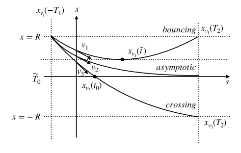
Figure 4.1. Bouncing, asymptotic and crossing vectors

For type 1 manifolds, the condition (3.4) is established in the proposition below (as for bouncing vectors):

Proposition 4.2.

For any $R>0$ sufficiently small (see Lemma 4.4 for the domain $R$ can take), there exists $Q=Q(R)>1$ independent of $t$ such that for any $v\in T^{1}M$ with $x_{v}(0)=R$ and $\phi_{v}(0)<0$,

1. if $v$ is a bouncing vector relative to $N_{R}(\widetilde{T}_{0})$, then for $\tau\in[0,\tilde{t}\,]$ we have

   $$Q^{-1}(\tau+1)^{-\frac{2}{m}}\leq x_{v}(\tau)\leq Q(\tau+1)^{-\frac{2}{m}};$$

   $$Q^{-1}[(\tau+1)^{-\frac{m+2}{m}}-(\tilde{t}+1)^{-\frac{m+2}{m}}]\leq|\phi_{v}(\tau)|\leq Q[(\tau+1)^{-\frac{m+2}{m}}-(\tilde{t}+1)^{-\frac{m+2}{m}}];$$

2. if $v$ is an asymptotic vector relative to $N_{R}(\widetilde{T}_{0})$, then for $\tau\in[0,\infty)$ we have

   $$Q^{-1}(\tau+1)^{-\frac{2}{m}}\leq x_{v}(\tau)\leq Q(\tau+1)^{-\frac{2}{m}};$$

   $$Q^{-1}[(\tau+1)^{-\frac{m+2}{m}}]\leq|\phi_{v}(\tau)|\leq Q[(\tau+1)^{-\frac{m+2}{m}}];$$

3. if $v$ is a crossing vector relative to $N_{R}(\widetilde{T}_{0})$, then for $\tau\in[0,t_{0}]$, we have

   $$Q^{-1}[(\tau+1)^{-\frac{2}{m}}-(t_{0}+1)^{-\frac{2}{m}}]\leq x_{v}(\tau)\leq Q[(\tau+1)^{-\frac{2}{m}}-(t_{0}+1)^{-\frac{2}{m}}];$$

   $$Q^{-1}(\tau+1)^{-\frac{m+2}{m}}\leq|\phi_{v}(\tau)|\leq Q(\tau+1)^{-\frac{m+2}{m}}.$$

Remark.

Proposition 4.2 is more general than (3.4). The lower bound of $|\phi_{v}(\tau)|$ is not necessary for deriving Proposition 3.4.

We begin by collecting relevant lemmas to prove this proposition, the first of which concerns with a general property of Riccati solutions.

Lemma 4.3.

There exists $R_{0}=R_{0}(C,m)$ such that for any $R\in[0,R_{0}]$, and any solution $U:[0,R]\to M_{n-1}(\mathbb{R})$ of the following Riccati equation

(4.3) $$U^{\prime}+U^{2}-Cx^{m}I_{n-1}=0,\quad U(0)=0,$$

we have

$$\frac{Cx^{m+1}}{2(m+1)}I_{n-1}\leq U(x)\leq\frac{Cx^{m+1}}{m+1}I_{n-1}.$$

Proof.

Let $\lambda:[0,R]\to\mathbb{R}$ be the solution of

$$\lambda^{\prime}+\lambda^{2}-Cx^{m}=0,\quad\lambda(0)=0.$$

Then $\lambda I_{n-1}$ satisfies (4.3). Since the solution of any first order ODE is unique, we have $U=\lambda I_{n-1}$.

Now we estimate $\lambda$. Since $\lambda^{\prime}=Cx^{m}-\lambda^{2}\leq Cx^{m}$, we have

$$\lambda(x)=\int_{0}^{x}\lambda^{\prime}(s)ds\leq\int_{0}^{x}Cs^{m}ds=\frac{C}{m+1}x^{m+1}.$$

establishing the required the upper bound on $U(x)$.

For the lower bound, let ${\displaystyle R_{0}:=\Big{(}\frac{(m+1)^{2}}{2C}\Big{)}^{\frac{1}{m+2}}}$. Then for any $x\in[0,R_{0}]$ the upper bound for $\lambda(x)$ gives

$$\lambda^{\prime}=Cx^{m}-\lambda^{2}\geq Cx^{m}-\frac{C^{2}}{(m+1)^{2}}x^{2m+2}\geq\frac{C}{2}x^{m}$$

which then gives ${\displaystyle\lambda(x)=\int_{0}^{x}\lambda^{\prime}(s)ds\geq\frac{C}{2(m+1)}x^{m+1}}$ as required. ∎

Recalling the notations $x_{v}(\tau):=x(\gamma_{v}(\tau))$ and $\phi_{v}(\tau):=\phi(\gamma_{v}^{\prime}(\tau))$ from (2.2), the following lemma uses the curvature bound (4.2) to compare $x^{\prime\prime}_{v}$ with $x_{v}^{m+1}$ for any shadowing vector $v$.

Lemma 4.4.

There exists $R_{1}=R_{1}(C_{1},C_{2},m)>0$ such that for any $R\in[0,R_{1}]$ and any $v$ with $x_{v}(0)<R$, we have

$$\frac{C_{2}}{4m+4}x_{v}^{m+1}\leq x_{v}^{\prime\prime}\leq\frac{C_{1}}{m+1}x_{v}^{m+1},$$

as long as $|x_{v}|<R$. In particular, $x_{v}$ is strictly convex and positive.

Proof.

Since $-C_{1}x(v)^{m}\leq K_{\perp}(v)\leq-C_{2}x(v)^{m},$ we have

$$-C_{1}x^{m}I_{n-1}\leq\mathcal{K}(X)\leq-C_{2}x^{m}I_{n-1}.$$

Using $R_{0}$ from the previous lemma, we claim that we can take

$$R_{1}:=\min\{R_{0}(C_{1},m),R_{0}(C_{2},m)\}.$$

For $i=1,2$ and $R\in(0,R_{1})$, let $U_{i}:[0,R]\to M_{n-1}(\mathbb{R})$ be the solution of

$$U_{i}^{\prime}+U_{i}^{2}-C_{i}x^{m}I_{n-1}=0,\quad U_{i}(0)=0.$$

By the main theorem in [EH90], the solutions satisfy

$$U_{2}\leq U\leq U_{1}$$

on $[0,R]$. By Lemmas 2.2 and 4.3 and Remark 3.3, we have

$$x^{\prime\prime}_{v}(x)\geq\frac{\lambda_{1}(s,x_{v})}{2}\geq\frac{C_{2}}{4m+4}x_{v}^{m+1}$$

and

$$x^{\prime\prime}_{v}(x)\leq\lambda_{n-1}(s,x_{v})\leq\frac{C_{1}}{m+1}x_{v}^{m+1}.$$

If $x_{v}$ vanishes somewhere in $(0,t)$, and assume $\tilde{a}$ is the smallest zero of $x_{w}$ in $(0,t)$. It is clear that $x_{w}^{\prime}(\tilde{a})\leq 0$ because if $x_{v}^{\prime}(\tilde{a})=0$, then it would imply $x_{v}\subseteq\widetilde{T}_{0}$ which is impossible. Thus $x_{v}^{\prime}(\tilde{a})<0$, and denote by $\tilde{b}$ the next zero of $x_{v}$. Then $x_{v}$ is a geodesic connecting two distinct points on a totally geodesic submanifold $\widetilde{T}_{0}$, which would imply $x_{v}\subseteq\widetilde{T}_{0}$, again resulting in a contradiction. Therefore, $x_{v}(\tau)$ is positive for all $\tau\in[0,t]$. ∎

We also need the following auxiliary lemma.

Lemma 4.5.

Let $f:[a,b]\to\mathbb{R}$ be a piecewise smooth strictly decreasing function with finitely many discontinuities. Assume that $f(b)>0$ and that there exists $0<Q_{1}<Q_{2},\alpha>0,\beta\in(0,1)$ with $\alpha\beta>1$ such that

$$-Q_{2}(f(\tau)^{\alpha}-f(b)^{\alpha})^{\beta}\leq f^{\prime}(\tau)\leq-Q_{1}(f(\tau)^{\alpha}-f(b)^{\alpha})^{\beta}$$

when $f$ is smooth at $\tau$. Then exists a constant $Q_{0}=Q_{0}(\alpha,\beta)>0$ independent of $a,b,f$ such that

$$(f(a)^{1-\alpha\beta}+Q_{2}(\alpha\beta-1)(\tau-a))^{\frac{1}{1-\alpha\beta}}\leq f(\tau)\leq Q_{0}(f(a)^{1-\alpha\beta}+Q_{1}(\alpha\beta-1)(\tau-a))^{\frac{1}{1-\alpha\beta}}$$

for all $\tau\in[a,b]$.

Proof.

We firstly consider the lower bound of $f$. Firstly we have

(4.4) $$\frac{d}{d\tau}f(\tau)^{1-\alpha\beta}=(\alpha\beta-1)(-f^{\prime})f(\tau)^{-\alpha\beta}\leq Q_{2}(\alpha\beta-1),$$

whenever $f$ is smooth. Thus

$$f(\tau)^{1-\alpha\beta}\leq f(a)^{1-\alpha\beta}+Q_{2}(\alpha\beta-1)(\tau-a).$$

Hence

$$f(\tau)\geq(f(a)^{1-\alpha\beta}+Q_{2}(\alpha\beta-1)(\tau-a))^{\frac{1}{1-\alpha\beta}}.$$

Now we compute the upper bound. Similar to the lower bound, we get

$$\frac{d}{d\tau}f(\tau)^{1-\alpha\beta}=(\alpha\beta-1)(-f^{\prime})f(\tau)^{-\alpha\beta}\geq Q_{1}(\alpha\beta-1)\left(1-\left(\frac{f(b)}{f(\tau)}\right)^{\alpha}\right)^{\beta},$$

whenever $f$ is smooth.

We then define an auxiliary piecewise smooth function

$$g(\tau):=\left(\frac{f(\tau)}{f(b)}\right)^{1-\alpha\beta}$$

which is strictly increasing on $[a,b]$ with $g(a)\in(0,1)$ and $g(b)=1$. Moreover,

(4.5) $$\frac{dg}{d\tau}\geq Q_{1}(\alpha\beta-1)f(b)^{\alpha\beta-1}\left(1-g^{\frac{\alpha}{\alpha\beta-1}}\right)^{\beta}.$$

Let $\tilde{g}$ be the solution of the ODE

(4.6) $$\frac{d\tilde{g}}{d\tau}=Q_{1}(\alpha\beta-1)f(b)^{\alpha\beta-1}\left(1-\tilde{g}^{1/\beta}\right)^{\beta},\quad\quad\tilde{g}(a)=g(a).$$

Since $\frac{\alpha}{\alpha\beta-1}>\frac{1}{\beta}$, from (4.5) and (4.6) we know that $\tilde{g}^{\prime}(a)<g^{\prime}(a)$, thus $\tilde{g}(\tau)<g(\tau)$ when $\tau$ is slightly larger than $a$. In fact, we have $\tilde{g}(\tau)<g(\tau)$ for all $\tau\in(a,b)$. This is because if $\tilde{g}(\tau)\geq g(\tau)$ for some $\tau$, then we can define $\tau_{0}\in(a,b)$ to be the smallest $\tau$ with $\tilde{g}(\tau)=g(\tau)$. Since $\tilde{g}(\tau)<g(\tau)$ on $(a,\tau_{0})$, the condition $\tilde{g}(\tau_{0})=g(\tau_{0})$ implies $\tilde{g}^{\prime}(\tau_{0})\geq g^{\prime}(\tau_{0})$. On the other hand, the condition $\tilde{g}(\tau_{0})=g(\tau_{0})$ considered with (4.5) and (4.6) implies $\tilde{g}^{\prime}(\tau_{0})<g^{\prime}(\tau_{0})$, deriving a contradiction. Thus $\tilde{g}<g$ on $(a,b)$.

By (4.6), we have

$$\left(1-\tilde{g}^{1/\beta}\right)^{-\beta}\frac{d\tilde{g}}{d\tau}=Q_{1}(\alpha\beta-1)f(b)^{\alpha\beta-1}.$$

Thus for any $\tau\in[a,b]$,

(4.7) $$F_{\beta}(\tilde{g}(\tau))-F_{\beta}(\tilde{g}(a))=Q_{1}(\alpha\beta-1)f(b)^{\alpha\beta-1}(\tau-a),$$

where

$$F_{\beta}(x):=\int_{0}^{x}(1-y^{1/\beta})^{-\beta}\,dy.$$

It is clear that $F_{\beta}$ is convex on $[0,1]$, thus $F^{\prime}_{\beta}(x)\geq F^{\prime}_{\beta}(0)=1$ for $x\in[0,1]$. Hence for any $x\in[0,1]$,

(4.8) $$F_{\beta}(x)\geq x.$$

On the other hand, since $F_{\beta}$ is convex and increasing, $F_{\beta}(x)/x$ is also increasing on $[0,1]$. Thus for any $x\in(0,1)$

(4.9) $$\frac{F_{\beta}(x)}{x}\leq F_{\beta}(1)=\int_{0}^{1}t^{\beta-1}(1-t)^{-\beta}dt=\mathcal{B}(\beta,1-\beta)<\infty,$$

where $\mathcal{B}$ is the beta function. By combining (4.7), (4.8), and (4.9), we get

$$\mathcal{B}(\beta,1-\beta)\tilde{g}(\tau)-\tilde{g}(a)\geq Q_{1}(\alpha\beta-1)f(b)^{\alpha\beta-1}(\tau-a).$$

Hence

$$\mathcal{B}(\beta,1-\beta)f(\tau)^{1-\alpha\beta}-f(a)^{1-\alpha\beta}\geq Q_{1}(\alpha\beta-1)(\tau-a).$$

Setting $Q_{0}:=\mathcal{B}(\beta,1-\beta)^{\frac{1}{\alpha\beta-1}}$, we have

$$f(\tau)\leq Q_{0}(f(a)^{1-\alpha\beta}+Q_{1}(\alpha\beta-1)(\tau-a))^{\frac{1}{1-\alpha\beta}}.$$

This completes the proof. ∎

We are now ready to prove Proposition 4.2.

Proof of Proposition 4.2.

For simplicity we will use $x$ to denote $x_{v}$. We will also use $Q$ to denote a generic constant that may need to be updated; this will be made more clear as they show up in the proof.

Case 1: $v$ is a bouncing vector. We will first prove the lower bound for $x(\tau)$ when $\tau\in[0,\tilde{t}\,]$. Noting that $x^{\prime}(\tilde{t})=0$, by Lemma 4.4, we have

$$x^{\prime}(\tau)^{2}=-\int_{\tau}^{\tilde{t}}2x^{\prime}x^{\prime\prime}ds\leq\frac{2C_{1}}{m+1}\int_{\tau}^{\tilde{t}}-x^{\prime}x^{m+1}ds\leq\frac{2C_{1}}{(m+1)^{2}}(x(\tau)^{m+2}-x(\tilde{t})^{m+2})$$

and

$$x^{\prime}(\tau)^{2}=-\int_{\tau}^{\tilde{t}}2x^{\prime}x^{\prime\prime}ds\geq\frac{C_{2}}{2m+2}\int_{\tau}^{\tilde{t}}-x^{\prime}x^{m+1}ds\geq\frac{C_{2}}{2(m+2)^{2}}(x(\tau)^{m+2}-x(\tilde{t})^{m+2}).$$

By taking $\alpha=m+2,\beta=1/2,f(a)=R$ in Lemma 4.5, we know that there exists $Q$ independent of $v,t$ such that for any $\tau\in[0,\tilde{t}]$,

$$Q^{-1}(\tau+1)^{-\frac{m}{2}}\leq x(\tau)\leq Q(\tau+1)^{-\frac{m}{2}}.$$

For $\phi$, recall that $x^{\prime}=\sin\phi$. Thus $(\sin\phi)^{\prime}=x^{\prime\prime}$. By Lemma 4.4 we have

$$Q^{-1}(\tau+1)^{-\frac{2(m+1)}{m}}\leq\frac{C_{2}}{4m+4}x^{m+1}\leq(\sin\phi)^{\prime}\leq\frac{C_{1}}{m+1}x^{m+1}\leq Q(\tau+1)^{-\frac{2(m+1)}{m}}.$$

Taking the integral on $[\tau,\tilde{t}]$, we get

$$Q^{-1}[(\tau+1)^{-\frac{m+2}{m}}-(\tilde{t}+1)^{-\frac{m+2}{m}}]\leq\sin\phi(\tau)\leq Q[(\tau+1)^{-\frac{m+2}{m}}-(\tilde{t}+1)^{-\frac{m+2}{m}}].$$

Since $\sin\phi/\phi\in[2/\pi,1]$, we have the same bounds for $\phi$.

Case 2: $v$ is an asymptotic vector. It is not hard to see that the above argument is valid when $\tilde{t}=\infty.$

Case 3: $v$ is a crossing vector. Denote by $a(t):=-\sin\phi(t)$. By Lemma 4.4, we know that whenever $|x|\leq R$,

$$\frac{C_{2}}{4m+4}x^{m+1}\leq x^{\prime\prime}\leq\frac{C_{1}}{m+1}x^{m+1}.$$

Thus

$$\frac{C_{2}}{4m+4}(-x^{\prime}x^{m+1})\leq-x^{\prime}x^{\prime\prime}\leq\frac{C_{1}}{m+1}(-x^{\prime}x^{m+1}).$$

Taking integral, we get

(4.10) $$\frac{C_{2}}{(2m+4)^{2}}x^{m+2}\leq a^{2}-a(t_{0})^{2}\leq\frac{C_{1}}{(m+1)^{2}}x^{m+2}.$$

Hence

$$\frac{(m+1)^{2}}{C_{1}}(a^{2}-a(t_{0})^{2})\leq x^{m+2}\leq\frac{(2m+4)^{2}}{C_{2}}(a^{2}-a(t_{0})^{2})$$

Since $x^{\prime}=-a$, we have $a^{\prime}=-x^{\prime\prime}$. Thus there exists $C>c>0$ independent of $v,t$ such that

$$-C(a^{2}-a(t_{0})^{2})^{\frac{m+1}{m+2}}\leq a^{\prime}\leq-c(a^{2}-a(t_{0})^{2})^{\frac{m+1}{m+2}}.$$

Setting $\alpha=2,\beta=\frac{m+1}{m+2}$ in Lemma 4.5, we have

(4.11) $$(a(0)^{-\frac{m}{m+2}}+C(\tau-a))^{-\frac{m+2}{m}}\leq a(\tau)\leq Q_{0}(a(0)^{-\frac{m}{m+2}}+c(\tau-a))^{-\frac{m+2}{m}}$$

Since $x_{v}(0)=R$ and $a(0)>0$, by compactness, $a(0)$ has a uniform lower bound depending on $R$. Thus we have

$$Q^{-1}(\tau+1)^{-\frac{m+2}{m}}\leq|\phi(\tau)|\leq Q(\tau+1)^{-\frac{m+2}{m}}.$$

Similar to Case 1, the bound of $x$ comes from $x(\tau)=\int_{\tau}^{t_{0}}a(s)ds$ and (4.11). ∎

Remark 4.6.

Note that we did not use the full strength of Lemma 4.5 in the above proof; that is, $x(\tau)$ had no discontinuities. The next section will make similar use of Lemma 4.5 applied to a function with discontinuities.

5. Estimates for type 2 surfaces

In this section, we consider a different setting considered by Gerber and Niţică [GN99] as well as Gerber and Wilkinson [GW99] where $M=S$ is a complete nonpositively curved surface, and $T_{0}$ is a closed geodesic of some length $\gamma_{0}$ on which the Gaussian curvature $K$ vanishes to order $m-1$. Namely, if $(s,x)$ are the Fermi coordinates along $\widetilde{T}_{0}$, there exists $C_{1},C_{2},\varepsilon>0$ and an interval $L=[0,\gamma_{1}]$ for some $\gamma_{1}\in(0,\gamma_{0})$ such that

(5.1) $$-C_{1}|x|^{m}\leq K(s,x)\leq 0$$

for all $|x|<\varepsilon$ and for all $s\in\mathbb{R}$ and

(5.2) $$-C_{1}|x|^{m}\leq K(s,x)\leq-C_{2}|x|^{m}$$

for all $|x|<\varepsilon$ and $s\in\tilde{L}$. In order to simplify the argument whenever applicable, we will adopt the notation for the Riemannian metric $g$ specified for a surface introduced in Remark 2.3.

Remark 5.1.

Compared to the assumption in the previous section, the underlying manifold considered in this section is 2-dimensional and the curvature assumption near $T_{0}$ is weakened: the neighborhood of only a small subset $L$ of $T_{0}$ is assumed to satisfy the uniform curvature bound as in (4.2).

On the complement of $L$ in $T_{0}$ and its neighborhood, only the trivial upper bound (ie, zero) is imposed on the curvature. Despite the weaker assumption on the curvature, the low dimensionality of the manifold enables us a finer analysis to prove the similar estimates (3.4) on $x_{w}$ and $\phi_{w}$ for $w=\Pi_{t,R}(\mathsf{v})$. Furthermore, unlike the previous section where $R$ from the definition (3.1) of the shadowing map $\Pi_{t,R}$ had to be carefully chosen, this setting is less sensitive to choice of $R$.

Remark 5.2.

One can continue using techniques developed in the previous section to study the bouncing, asymptotic and crossing vectors. Nevertheless, in the surface setting, the geometric potential estimates were well-studied in [GW99]. Without deviating from the main goal and to simplify the argument in this section, we will only focus on shadowing vectors $w=\Pi_{t,R}(\mathsf{v})$.

The goal of this section is to show that under this different set of assumptions the shadowing vector $w=\Pi_{t,R}(\mathsf{v})$ satisfies the estimates on $x_{w}$ and $\phi_{w}$ as claimed in (3.4). Recalling that $\gamma_{0}$ is the length of $T_{0}$, we state it as a proposition below, which is the analogue of Proposition 4.2.

Proposition 5.3.

There exists $Q=Q(R)>1$ independent of $t$ such that for any shadowing vector $w=\Pi_{t,R}(\mathsf{v})$ and $\tau\in[0,\tilde{t}]$ we have

$$Q^{-1}(\tau+1)^{-\frac{2}{m}}\leq x_{w}(\tau)\leq Q(\tau+1)^{-\frac{2}{m}},$$

and

$$|\phi_{w}(\tau)|\leq Q[(\tau+1)^{-\frac{m+2}{m}}-(\tilde{t}+1)^{-\frac{m+2}{m}}],$$

and for any $\tau\in[0,\tilde{t}-2\sqrt{2}\gamma_{0}]$,

$$|\phi_{w}(\tau)|\geq Q^{-1}[(\tau+1)^{-\frac{m+2}{m}}-(\tilde{t}+1)^{-\frac{m+2}{m}}].$$

Remark 5.4.

We do not expect the lower bound of $|\phi_{w}(\tau)|$ to hold for all $\tau\in[0,\tilde{t}\,]$ since we have little control of the metric near $\gamma(\tilde{t})$. For instance, when the metric near $\gamma(\tilde{t})$ is isometric to the surface of revolution of $1+x^{2m}$, by Proposition 3.1 we know that $\phi_{w}(\tau)$ is of the same scale as $(\tau+1)^{-\frac{m+1}{m}}-(\tilde{t}+1)^{-\frac{m+1}{m}}$ when $\tau$ is near $\tilde{t}$.

In order to prove the proposition, we need to exploit the assumptions on $K(s,x)$ and establish a few auxiliary lemmas. Consider any $w=\Pi_{t,R}(\mathsf{v})$ for some $t,R>0$ and $v\in\mathrm{Sing}$. Recall that $\tilde{t}\in[0,t]$ is the smallest number in which $x_{w}(\tau)$ attains the minimum. We can decompose $[0,\tilde{t}]$ into subintervals $I_{i}=[t_{i},t^{\prime}_{i}]$ and $I^{\prime}_{i}=(t^{\prime}_{i},t_{i+1})$ for $i=0,1,\cdots,n$ so that

$$s(\gamma_{w}(\tau))\in\tilde{L}\text{ when }\tau\in I_{i}$$

and

$$s(\gamma_{w}(\tau))\notin\tilde{L}\text{ when }\tau\in I^{\prime}_{i};$$

see Figure 5.1. Notice that $\tilde{t}\geq t_{n}$, thus $I_{n}$ is not empty (though it may be arbitrarily short), but $I^{\prime}_{n}$ may be empty.

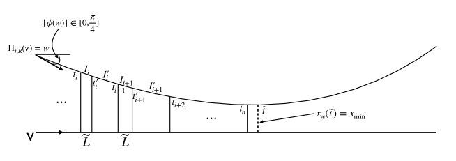
Figure 5.1. Division into $I_{i}$ and $I_{i}^{\prime}$.

Since the angle $\phi_{w}(\tau)$ satisfies $|\phi_{w}(\tau)|\in[0,\pi/4]$ for any $\tau\in[0,t]$ from Lemma 3.1, there exists $N\in\mathbb{N}$ so that

$$\min\limits_{i}|I_{i}|\geq\frac{1}{N}\max\limits_{i}|I^{\prime}_{i}|$$

where the maximum is taken over all possible $i$ and the minimum is taken over $i$ in $\{1,\ldots,n\}$ if $t_{0}\in I_{n}^{\prime}$ (i.e. $I_{n}^{\prime}$ is nonempty) or else (i.e. $\tilde{t}\in I_{n}$ and $I_{n}^{\prime}$ is empty) in $\{1,\ldots,n-1\}$ in order to exclude $|I_{n}|$ which could be arbitrarily small.

The following lemma shows $x_{w}^{\prime\prime}(\tau)$ admits a similar bound as in Lemma 4.4 when $\tau$ belongs to $I_{i}$ for some $i$.

Lemma 5.5.

There exists $C_{0}>0$ independent of $w$ such that

$$0\leq x_{w}^{\prime\prime}\leq C_{0}x_{w}^{m+1}$$

for all $\tau\in[0,\tilde{t}\,]$. Moreover, there exists $c_{0}\in(0,C_{0})$ such that whenever $\tau\in I_{i}$ for some $i$, we also have the lower bound

$$x_{w}^{\prime\prime}\geq c_{0}x_{w}^{m+1}.$$

Proof.

Since $G_{xx}=-KG\leq 2C_{1}x_{w}^{m}$ with $G_{x}(s,0)=0$ for all $s$, thus $G_{x}(s,x_{w})\leq 2C_{1}(m+1)^{-1}x_{w}^{m+1}$. Let $C_{0}:=2C_{1}(m+1)^{-1}$. By (2.6),

$$x^{\prime\prime}_{w}=\frac{G_{x}}{G}\cos^{2}\phi_{w}\leq\frac{G_{x}}{G}\leq C_{0}x_{w}^{m+1}.$$

For $t\in I_{i}$, we have $G_{xx}=-KG\geq C_{2}x_{w}^{m}$, thus $G_{x}(s,x_{w})\geq C_{2}(m+1)^{-1}x_{w}^{m+1}$. Let $c_{0}:=C_{2}(2m+2)^{-1}$. By Lemma 3.1 (1), we have

$$x^{\prime\prime}_{w}=\frac{G_{x}}{G}\cos^{2}\phi_{w}\geq\frac{G_{x}}{\sqrt{2}G}\geq c_{0}x_{w}^{m+1}.$$

This completes the proof. ∎

The following lemma we let ${\displaystyle t^{\prime\prime}_{i}:=\frac{t_{i}+t^{\prime}_{i}}{2}}$. For simplicity, in the remaining part of this section, we abbreviate $x=x_{w}$ and $\phi=\phi_{w}$ where $w=\Pi_{t,R}(\mathsf{v})$ for any $\mathsf{v}\in\mathrm{Sing}$ and $t,R>0$.

Lemma 5.6.

For any $i$ with $|I_{i}|\geq\gamma_{1}$ (namely, those $I_{i}$ not containing 0 or $t_{0}$), we have

1. ${\displaystyle\int_{t^{\prime\prime}_{i}}^{t^{\prime}_{i}}-x^{\prime}x^{m+1}ds\geq\frac{1}{2N+1}\int_{t^{\prime\prime}_{i}}^{t_{i+1}}-x^{\prime}x^{m+1}ds.}$

2. ${\displaystyle\int_{\tau}^{t^{\prime}_{i}}-x^{\prime}x^{m+1}ds\geq\frac{1}{2N+1}\int_{\tau}^{t_{i+1}}-x^{\prime}x^{m+1}ds}$ for any $\tau\in[t_{i},t^{\prime\prime}_{i}]$.

Proof.

For (1) consider any $s\in[t^{\prime\prime}_{i},t^{\prime}_{i}]$ and $s^{\prime}\in[t^{\prime}_{i},t_{i+1}]$. Since $x$ is convex and decreasing, we have $-x^{\prime}(s)\geq-x^{\prime}(s^{\prime})$ and $x(s)\geq x(s^{\prime})$. In particular,

$$-x^{\prime}(s)x(s)^{m+1}\geq-x^{\prime}(s^{\prime})x(s^{\prime})^{m+1}.$$

Since ${\displaystyle\min_{i}|I_{i}|\geq\frac{1}{N}\max_{i}|I^{\prime}_{i}|}$, we can divide $I^{\prime}_{i}$ into $2N$ subintervals of the same length. The integral on each subinterval, whose length is at most $|I_{i}|/2$, is no more than that on $[t^{\prime\prime}_{i},t^{\prime}_{i}]$. Hence

$$\int_{t^{\prime\prime}_{i}}^{t_{i+1}}-x^{\prime}x^{m+1}ds = \int_{t^{\prime\prime}_{i}}^{t^{\prime}_{i}}-x^{\prime}x^{m+1}ds+\int_{t^{\prime}_{i}}^{t_{i+1}}-x^{\prime}x^{m+1}ds$$

$$\leq \int_{t^{\prime\prime}_{i}}^{t^{\prime}_{i}}-x^{\prime}x^{m+1}ds+2N\int_{t^{\prime\prime}_{i}}^{t^{\prime}_{i}}-x^{\prime}x^{m+1}ds$$

$$= (1+2N)\int_{t^{\prime\prime}_{i}}^{t^{\prime}_{i}}-x^{\prime}x^{m+1}ds.$$

For (2), by (1) we have

$$\int_{\tau}^{t^{\prime}_{i}}-x^{\prime}x^{m+1}ds = \int_{\tau}^{t^{\prime\prime}_{i}}-x^{\prime}x^{m+1}ds+\int_{t^{\prime\prime}_{i}}^{t^{\prime}_{i}}-x^{\prime}x^{m+1}ds$$

$$\geq \int_{\tau}^{t^{\prime\prime}_{i}}-x^{\prime}x^{m+1}ds+\frac{1}{2N+1}\int_{t^{\prime\prime}_{i}}^{t_{i+1}}-x^{\prime}x^{m+1}ds$$

$$\geq \frac{1}{2N+1}\int_{\tau}^{t_{i+1}}-x^{\prime}x^{m+1}ds.$$

∎

Lemma 5.7.

There exists $C_{3}>0$ such that for any $i$ and $\tau\in[t_{i},t^{\prime\prime}_{i}]$,

$$x^{\prime}(\tau)\leq-2C_{3}\sqrt{x(\tau)^{m+2}-x(\,\tilde{t}\,)^{m+2}}.$$

Proof.

If $\tilde{t}\in I^{\prime}_{n}$, by Lemmas 5.5 and 5.6, we have

$$x^{\prime}(\tau)^{2} = \int_{\tau}^{\tilde{t}}-2x^{\prime}x^{\prime\prime}ds\geq 2c_{0}\left(\int_{\tau}^{t^{\prime}_{i}}-x^{\prime}x^{m+1}ds+\sum_{k=i+1}^{n}\int_{t_{k}}^{t^{\prime}_{k}}-x^{\prime}x^{m+1}ds\right)$$

$$\geq \frac{2c_{0}}{2N+1}\left(\int_{\tau}^{t_{i+1}}-x^{\prime}x^{m+1}ds+\sum_{k=i+1}^{n-1}\int_{t_{k}}^{t_{k+1}}-x^{\prime}x^{m+1}ds+\int_{t_{n}}^{\tilde{t}}-x^{\prime}x^{m+1}ds\right)$$

$$\geq \frac{2c_{0}}{2N+1}\int_{\tau}^{t_{0}}-x^{\prime}x^{m+1}ds\geq\frac{2c_{0}}{(m+2)(2N+1)}(x(\tau)^{m+2}-x(\,\tilde{t}\,)^{m+2}).$$

Similarly, if $\tilde{t}\in I_{n}$, we have

$$x^{\prime}(\tau)^{2} = \int_{\tau}^{\tilde{t}}-2x^{\prime}x^{\prime\prime}ds$$

$$\geq 2c_{0}\left(\int_{\tau}^{t^{\prime}_{i}}-x^{\prime}x^{m+1}ds+\sum_{k=i+1}^{n-1}\int_{t_{k}}^{t^{\prime}_{k}}-x^{\prime}x^{m+1}ds+\int_{t_{n}}^{\tilde{t}}-x^{\prime}x^{m+1}ds\right)$$

$$\geq \frac{2c_{0}}{2N+1}\left(\int_{\tau}^{t_{i+1}}-x^{\prime}x^{m+1}ds+\sum_{k=i+1}^{n-1}\int_{t_{k}}^{t_{k+1}}-x^{\prime}x^{m+1}ds+\int_{t_{n}}^{\tilde{t}}-x^{\prime}x^{m+1}ds\right)$$

$$\geq \frac{2c_{0}}{2N+1}\int_{\tau}^{\tilde{t}}-x^{\prime}x^{m+1}ds\geq\frac{2c_{0}}{(m+2)(2N+1)}(x(\tau)^{m+2}-x(\,\tilde{t}\,)^{m+2}).$$

We finish the proof by taking $C_{3}:=2^{-1/2}c_{0}^{1/2}(m+2)^{-1/2}(2N+1)^{-1/2}$. ∎

Proof of Proposition 5.3.

As did in Proposition 4.2, we will use $Q$ to denote a generic constant. The desired lower bound for $x(\tau)$ can be established just as done in Proposition 4.2. This is because the upper bound $0\leq x_{w}^{\prime\prime}\leq C_{0}x_{w}^{m+1}$ from Lemma 5.5 holds for all $\tau\in[0,\tilde{t}\,]$, and this is the only ingredient needed for the lower bound on $x(\tau)$ in Proposition 4.2. In particular, we have $x(\tau)\geq(R^{-\frac{m}{2}}+\sqrt{C_{0}}\tau)^{\frac{2}{m}}$ for all $\tau\in[0,\tilde{t}\,]$.

On the other hand, the desired upper bound for $x(\tau)$ is more difficult to obtain. The reason for introducing $t_{i}^{\prime\prime}$ and establishing Lemma 5.7 was to obtain the upper bound. We will prove the case where $0\in I^{\prime}_{0}$ and $\tilde{t}\in I_{n}$. Other cases are similar and we will comment on them at the end of the proof. We let $R_{t_{1}}>0$ be the lower bound on $x(t_{1})$ from the above paragraph.

First, define a sequence

$$S_{n}:=\Big{(}\sum_{k=1}^{n-1}|t^{\prime\prime}_{k}-t_{k}|\Big{)}+|\tilde{t}-t_{n}|,\leavevmode\nobreak\ S_{0}=0,\text{ and }S_{i}=\sum_{k=1}^{i}|t^{\prime\prime}_{k}-t_{k}|.$$

Then we have $0=S_{0}<S_{1}<\cdots<S_{n-1}<S_{n}$. Define a function $f:[0,S_{n}]\to\mathbb{R}$ via

$$f(\tau):=x(\tau-S_{i}+t_{i+1})\text{ when }\tau\in(S_{i},S_{i+1}].$$

Then $f$ is a piecewise smooth function with discontinuities at each $S_{i}$. Moreover, Lemma 5.7 shows that $f$ is strictly decreasing function satisfying the assumption of Lemma 4.5 with $Q=C_{3}$. Thus by Lemma 4.5, there exists $Q_{0}>1$ such that

$$f(\tau)\leq Q_{0}(f(0)^{-\frac{m}{2}}+C_{3}m\tau)^{-\frac{2}{m}}\leq Q_{0}(R_{t_{1}}^{-\frac{m}{2}}+C_{3}m\tau)^{-\frac{2}{m}}$$

for all $\tau\in[0,S_{n}]$. In particular, this inequality provides an upper bound for $x(\tau)$ for $\tau\in[t_{i},t_{i}^{\prime\prime}]$ for $1\leq i\leq n$; here $t_{n}^{\prime\prime}$ should be replaced by $\tilde{t}$ when $i=n$.

For $\tau\in[t_{i}^{\prime\prime},t_{i+1}]$, we have ${\displaystyle\frac{S_{i}}{\tau}\geq\frac{1}{2N+2}}$ from the choice of $N$. Thus for $\tau\in[t_{i}^{\prime\prime},t_{i+1}]$,

$$x(\tau) \leq x(t_{i}^{\prime\prime})=f(S_{i})\leq Q_{0}(f(0)^{-\frac{m}{2}}+C_{3}mS_{i})^{-\frac{2}{m}}$$

$$\leq Q_{0}\left(R_{t_{1}}^{-m/2}+\frac{C_{3}m}{2N+2}\tau\right)^{-\frac{2}{m}}.$$

For the last remaining subset of the domain when $\tau\in[0,t_{1}]$, which is due to the assumption that $0\in I^{\prime}_{0}$, we have $t_{1}\leq\sqrt{2}|\gamma_{0}|$. Therefore,

$$x(\tau)\leq x(0)=R\leq R(\sqrt{2}|\gamma_{0}|+1)^{\frac{2}{m}}(\tau+1)^{-\frac{2}{m}}.$$

In sum, we can find $Q>0$ such that

$$x(\tau)\leq Q(\tau+1)^{-\frac{2}{m}}$$

for all $\tau\in[0,\tilde{t}\,]$.

For $\phi$, using (2.4) and Lemmas 3.1 (1) and 5.5, there exists $Q>0$ such that

$$\phi^{\prime}\leq\sqrt{2}\phi^{\prime}\cos\phi=\sqrt{2}x^{\prime\prime}\leq\sqrt{2}C_{0}x^{m+1}\leq Q(\tau+1)^{-\frac{2(m+1)}{m}}.$$

Thus we get the required upper bound for $\phi$:

$$|\phi(\tau)|=\left|\int_{\tau}^{\tilde{t}}\phi^{\prime}ds\right|\leq\int_{\tau}^{\tilde{t}}|\phi^{\prime}|ds\leq Q\int_{\tau}^{\tilde{t}}(s+1)^{-\frac{2(m+1)}{m}}ds\leq Q[(\tau+1)^{-\frac{m+2}{m}}-(\tilde{t}+1)^{-\frac{m+2}{m}}].$$

This completes the proof when $0\in I^{\prime}_{0}$ and $\tilde{t}\in I_{n}$.

Other remaining cases can be dealt similarly. When $0\in I_{0}$ and $\tilde{t}\in I_{n}$, then exactly the same proof works; in fact, there is no need to separately consider $\tau\in[0,t_{1}]$ like we did above. In the case where $\tilde{t}\in I_{n}^{\prime}$, we can use proceed just as we did above by bounding $x(\tau)$ above by $x(t_{n}^{\prime\prime})$ for $\tau\in[t_{n}^{\prime\prime},\tilde{t}\,]$.

Now we consider the lower bound of $|\phi|$. For any $\tau\in[0,\tilde{t}-2\sqrt{2}\gamma_{0}]$, the interval $[\tau,\tilde{t}\,]$ contains at least one $[t_{i},t^{\prime}_{i}]$. Let $l$ (resp. $L$) be the minimal (resp. maximal) $i$ with $[t_{i},t^{\prime}_{i}]\subset[\tau,\tilde{t}\,]$. We firstly compare the integrals of $x(s)^{m+1}$ on $[\tau,t_{l}]$ and $[t_{l},t_{l+1}]$. Since $|\phi|<\pi/4$,

(5.3) $$t_{l+1}-t_{l}\geq\gamma_{0}\geq\frac{t_{l}-\tau}{\sqrt{2}}.$$

Moreover, we have

$$\frac{t_{l+1}+1}{\tau+1}=1+\frac{t_{l+1}-\tau}{\tau+1}\leq 1+2\sqrt{2}\gamma_{0}.$$

Hence

$$x(t_{l+1})\geq Q(t_{l+1}+1)^{-2/m}\geq Q(\tau+1)^{-2/m}\geq Qx(\tau).$$

Together with (5.3), since $x$ is non-increasing, we get

(5.4) $$\int_{t_{l}}^{t_{l+1}}x(s)^{m+1}ds\geq(t_{l+1}-t_{l})x(t_{l+1})^{m+1}\geq Q\frac{t_{l}-\tau}{\sqrt{2}}x(\tau)^{m+1}\geq Q\int_{\tau}^{t_{l}}x(s)^{m+1}ds.$$

Notice that $\phi^{\prime}=x^{\prime\prime}/\cos\phi\geq x^{\prime\prime}$, and $|I_{i}|/|I_{j}|\in[1/\sqrt{2},\sqrt{2}]$ for any $i,j$. Thus by (5.4),

$$|\phi(\tau)| = \int_{\tau}^{\tilde{t}}\phi^{\prime}(s)ds\geq\int_{\tau}^{\tilde{t}}x^{\prime\prime}(s)ds\geq c_{0}\sum_{i=l}^{L}\int_{t_{i}}^{t^{\prime}_{i}}x(s)^{m+1}\,ds$$

$$\geq \frac{c_{0}}{N+1}\sum_{i=l}^{L-1}\int_{t_{i}}^{t_{i+1}}x(s)^{m+1}ds+\frac{c_{0}}{N+1+\sqrt{2}}\int_{t_{L}}^{\tilde{t}}x(s)^{m+1}ds$$

$$\geq Q\int_{\tau}^{\tilde{t}}x(s)^{m+1}ds\geq Q\int_{\tau}^{\tilde{t}}(s+1)^{-2(m+1)/m}ds$$

$$\geq Q[(\tau+1)^{-\frac{m+2}{m}}-(\tilde{t}+1)^{-\frac{m+2}{m}}].$$

∎

6. Geometric potentials

The aim of this section is to prove Theorem C. Let $M$ be a closed rank 1 nonpositively curved manifold, and ${\mathcal{F}=}(f_{t})_{t\in\mathbb{R}}$ denote the geodesic flow on $T^{1}M.$ Recall that the geodesic potential is defined via

$$\varphi^{u}(v):=-\lim_{t\to 0}\frac{1}{t}\log\det(df_{t}|_{E^{u}(v)})=-\frac{d}{dt}\Big{|}_{t=0}\log\det(df_{t}|_{E^{u}(v)}).$$

As indicated in [BCFT18, Section 7.2], it is convenient to consider the following auxiliary function whose time evolution is governed by a Riccati equation:

$$\psi^{u}(v):=-\lim_{t\to 0}\frac{1}{t}\log\det(J_{v,t}^{u})=-\frac{d}{dt}\Big{|}_{t=0}\log\det(J_{v,t}^{u}),$$

where $J_{v,t}^{u}:w\in v^{\perp}\mapsto J(t)\in(f_{t}v)^{\perp}$ and $J(t)$ is a unstable Jacobi field along $\gamma_{v}$ such that $J(0)=w$. We also have $\psi^{u}(v)=-\text{tr }U_{v}^{u}(0)$ where $U_{v}^{u}(t)$ is the shape operator of the unstable horoshpere $H^{u}(f_{t}v)$.

Let $\pi:T^{1}M\to M$ be the canonical projection. Its derivative $d\pi_{v}:T_{v}T^{1}M\to T_{\pi v}M$ sends $E^{u}(v)$ onto $v^{\perp}.$ We have $df_{t}=d\pi_{f_{t}v}^{-1}\circ J_{v,t}^{u}\circ d\pi_{v}$, and thus

(6.1) $$\det(df_{t}|_{E^{u}(v)})=\det(d\pi_{f_{t}v})^{-1}\det(J_{v,t}^{u})\det(d\pi_{v}).$$

Thus

$$\varphi^{u}(v)-\psi^{u}(v)=\frac{d}{dt}\Big{|}_{t=0}\log\det(d\pi_{f_{t}v}).$$

For any $t$, since $U_{v}^{u}(t)$ is symmetric, we can take an orthonormal basis $\{e_{i}(t)\}_{i=1}^{n-1}$ of $v^{\perp}$ so that $U_{v}^{u}(t)e_{i}(t)=\lambda_{i}(t)e_{i}(t)$ with $\lambda_{i}(t)\geq 0$. Since $||df_{t}(\xi)||_{S}=\|J_{\xi}(t)\|^{2}+\|J^{\prime}_{\xi}(t)\|^{2}$ for $\xi\in E_{v}^{u}$, for any $t$, we have an orthonormal basis $\{\xi_{i}(t)\}_{i=1}^{n-1}$ of $E_{f_{t}v}^{u}$, where $\xi_{i}(t)$ is determined by

$$J_{\xi_{i}}(t)=\frac{e_{i}(t)}{\sqrt{1+\lambda_{i}(t)^{2}}},\quad J^{\prime}_{\xi_{i}}(t)=\frac{\lambda_{i}(t)e_{i}(t)}{\sqrt{1+\lambda_{i}(t)^{2}}}.$$

Thus $d\pi_{f_{t}v}(\xi_{i}(t))=e_{i}(t)/\sqrt{1+\lambda_{i}(t)^{2}}$ and the matrix of $d\pi_{f_{t}v}$ with respect to these two orthonormal basis is $\text{diag}((1+\lambda_{i}(t)^{2})^{-1/2},\cdots,(1+\lambda_{i}(t)^{2})^{-1/2})$. Hence

(6.2) $$\log\det(d\pi_{f_{t}v})=\log\prod_{i=1}^{n-1}(1+\lambda_{i}(t)^{2})^{-1/2}=-\frac{1}{2}\log\det(I_{n-1}+U_{v}^{u}(t)^{2}).$$

Now we use the following Jacobi formula for $A:\mathbb{R}\to M_{n-1}$:

$$\frac{d}{dt}\det A(t)=\det A(t)\text{ tr}\left(A(t)^{-1}\frac{dA(t)}{dt}\right).$$

For simplicity, denote by $U=U_{v}^{u}$ and $I=I_{n-1}$. By (6.1) and (6.2), we have

$$\varphi^{u}(v)-\psi^{u}(v) = -\frac{1}{2}\text{ tr}\left[(I+U(0)^{2})^{-1}(U^{\prime}(0)U(0)+U(0)U^{\prime}(0))\right]$$

$$= -\frac{1}{2}\text{ tr}\left[(U(0)(I+U(0)^{2})^{-1}+(I+U(0)^{2})^{-1}U(0))U^{\prime}(0)\right]$$

$$= -\text{ tr}\left[U(0)(I+U(0)^{2})^{-1}U^{\prime}(0)\right]$$

Since $U^{\prime}+U^{2}+\mathcal{K}=0$, $U$ is positive semidefinite, and $|\text{tr}(AB)|\leq|\text{tr}(A)||\text{tr}(B)|$ if $A,B$ are positive semidefinite, we have

$$|\varphi^{u}(v)-\psi^{u}(v)| \leq \text{ tr}\left[U^{3}(0)(I+U(0)^{2})^{-1}\right]+\text{ tr}\left[U(0)(I+U(0)^{2})^{-1}(-\mathcal{K})\right]$$

$$\leq (\text{tr }U(0))^{3}+\text{ tr}\left[U(0)(I+U(0)^{2})^{-1}]\text{ tr}(-\mathcal{K})\right]$$

$$= -\psi^{u}(v)^{3}-\psi^{u}(v)(-\text{Ric}(v))\leq-\psi^{u}(v)(\psi^{u}(v)^{2}-\text{Ric}(v)),$$

When $v$ is sufficiently close to Sing, $-\psi^{u}(v)$ and $-\text{Ric}(v)$ are small nonnegative numbers, thus we have $\varphi^{u}(v)\approx\psi^{u}(v)$ near $\mathrm{Sing}$. We summarize the above discussion below:

Proposition 6.1.

Suppose $M$ is a closed rank 1 nonpositively curved manifold. Then we have

$$|\varphi^{u}(v)-\psi^{u}(v)|\leq-\psi^{u}(v)(\psi^{u}(v)^{2}-\text{Ric}(v)).$$

In particular, we have $\varphi^{u}(v)\approx\psi^{u}(v)$ near $\mathrm{Sing}$.

6.1. The proof of Theorem C

The strategy of the proof is to study the auxiliary function $\psi^{u}$ through the associated Riccati equation. We establish a version of Theorem C for $\psi^{u}$. Then Theorem C follows Proposition 6.1.

We remark that the additional Ricci curvature constrain is essential in our argument. In the higher dimension scenario, it is not sufficient only having normal curvature controlled. Nevertheless, for some special Riemannian metrics, namely, warped products, the normal curvature $K_{\perp}(v)$ and Ricci curvature ${\rm Ric}(v)$ are comparable. Since this observation is not on the mainstream of the current paper, we leave the proof in Appendix A.

Let $M$ be a type 1 manifold with order $m-1$ Ricci curvature bounds, that is, there exists $k_{0},K_{0}>0$ such that

(6.3) $$-K_{0}|x_{v}|^{m}\leq\text{Ric}(v)\leq-k_{0}|x_{v}|^{m}$$

for all $v$ with $|x_{v}|\leq\varepsilon$.

Proposition 6.2.

Assume $M$ satisfies the normal curvature bound (4.2) and Ricci curvature bound (6.3), then $-\psi^{u}(v)\approx|x_{v}|^{m/2}+|\phi_{v}|^{m/(m+2)}$. In particular, we have the same scale estimation for $|\varphi^{u}|$.

To prove Proposition 6.2, we need the following lemma.

Lemma 6.3.

Assume there exist $K_{1}>k_{1}>0$ so that

1. $-K_{1}^{2}T^{-2}\leq\text{Ric}(\gamma^{\prime}_{v}(t))\leq-k_{1}^{2}T^{-2}$ for all $t\in[-T,0]$, then there exist $K_{2}>k_{2}>0$ depending on $k_{1},K_{1}$ so that

   $$k_{2}T^{-1}\leq-\psi^{u}(v)\leq K_{2}T^{-1}.$$

2. $-K_{1}^{2}T^{-2}\leq\text{Ric}(\gamma^{\prime}_{v}(t))\leq 0$ for all $t\in[0,k_{1}T]$, and $k_{3}T^{-1}\leq-\psi^{u}(v)\leq K_{3}T^{-1}$, then there exist $K_{4}>k_{4}>0$ depending on $k_{1},K_{1},k_{3},K_{3}$ so that

   $$k_{4}T^{-1}\leq-\psi^{u}(\gamma^{\prime}_{v}(t))\leq K_{4}T^{-1},$$

   for all $t\in[0,k_{1}T].$

Proof.

Denote by $u(t)=\frac{1}{n-1}\text{tr}(U_{v}^{u}(t))$. Since $U_{v}^{u}$ is diagonalizable and all eigenvalues $\lambda_{i}(t)$ are nonnegative, by Cauchy-Schwartz we have

$$\text{tr}((U_{v}^{u})^{2})\leq(n-1)^{2}u^{2}\leq(n-1)\text{tr}((U_{v}^{u})^{2}).$$

Thus by Riccati equation,

$$u^{\prime}=\frac{\text{tr}((U_{v}^{u})^{\prime})}{n-1}=-\frac{\text{tr}((U_{v}^{u})^{2})}{n-1}-\frac{\text{Ric}(\dot{\gamma})}{n-1}\leq-u^{2}-\frac{\text{Ric}(\dot{\gamma})}{n-1}.$$

On the other hand, denote by $w(t)=(n-1)u(t)=\text{tr}(U_{v}^{u}(t)).$ We have

$$w^{\prime}=-\text{tr}((U_{v}^{u})^{2})-\text{Ric}(\dot{\gamma})\geq-w^{2}-\text{Ric}(\dot{\gamma}).$$

1. Compare $u$ with the solution of

   $$\bar{u}^{\prime}+\bar{u}^{2}-K_{1}^{2}T^{-2}=0,\,\,\bar{u}(-T)=+\infty\quad\Rightarrow\quad\bar{u}(0)=K_{1}T^{-1}\coth K_{1}.$$

   By the main theorem in [EH90], we have

   $$-\psi^{u}(v)=(n-1)u(0)\leq(n-1)\bar{u}(0)=:K_{2}T^{-1}.$$

   Compare $w$ with the solution of

   $$\bar{w}^{\prime}+\bar{w}^{2}-k_{1}^{2}T^{-2}=0,\,\,\bar{w}(-T)=0\quad\Rightarrow\quad\bar{w}(0)=k_{1}T^{-1}\tanh k_{1}.$$

   We have

   $$-\psi^{u}(v)=w(0)\geq\bar{w}(0)=:k_{2}T^{-1}.$$

2. Compare $u$ with the solution of

   $$\bar{u}^{\prime}+\bar{u}^{2}-K_{1}^{2}T^{-2}=0,\,\,\bar{u}(0)=K_{3}T^{-1}.$$

   We have

   $$\bar{u}(t)=K_{1}T^{-1}\coth(K_{1}T^{-1}t+\coth^{-1}(K_{3}/K_{1})).$$

   Since $\coth$ is decreasing, so does $\bar{u}$. For $t\in[0,k_{1}T]$, we get

   $$-\psi^{u}(\gamma^{\prime}_{v}(t))=(n-1)u(t)\leq(n-1)\bar{u}(t)\leq(n-1)\bar{u}(0)=:K_{4}T^{-1}.$$

   Compare $w$ with the solution of

   $$\bar{w}^{\prime}+\bar{w}^{2}=0,\,\,\bar{w}(0)=k_{3}T^{-1}\quad\Rightarrow\quad\bar{w}(t)=(t+k_{3}^{-1}T)^{-1}.$$

   For $t\in[0,k_{1}T]$,

   $$-\psi^{u}(\gamma^{\prime}_{v}(t))=w(t)\geq\bar{w}(t)\geq(k_{1}T+k_{3}^{-1}T)^{-1}=:k_{4}T^{-1}.$$

∎

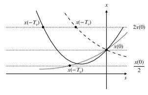
(a) Case 1

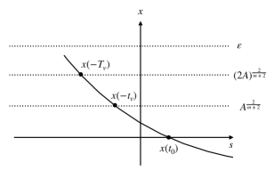
(b) Case 2

Figure 6.1. Proof of Proposition 6.2

Proof of Proposition 6.2.

We follow the main steps in the proof of [GW99, Lemma 3.3]. We use $x,\phi$ instead of $x_{v},\phi_{v}$ for simplicity.
Case 1: $v$ is bouncing or asymptotic. See Figure 6.1a. Since the asymptotic case is the bouncing case with $\tilde{t}=\infty$, we have only to consider the bouncing $v$. We may assume $0<x(0)\leq\varepsilon/2$. Denote by

$$T_{v}:=\max\{T>0:x(t)\in[x(0)/2,2x(0)],\forall-T\leq t\leq 0\}.$$

For any $t\in[-T_{v},0]$, we have $-K_{5}x(0)^{m}\leq\text{Ric}(\dot{\gamma}(t))\leq-k_{5}x(0)^{m}$. Moreover we have

Lemma 6.4.

$T_{v}\geq k_{6}x(0)^{-m/2}$ for some $k_{6}>0$ independent of $v$.

Proof.

Case 1: $x(-T_{v})=2x(0)$, and $x(t)$ is decreasing on $[-T_{v},0]$. By (4.4) with $\alpha=m+2,\beta=1/2$ , we have

$$x(0)^{-m/2}\leq(2x(0))^{-m/2}+K_{6}T_{v}.$$

Thus $T_{v}\geq k_{6}x(0)^{-m/2}$.

Case 2: $x(-T_{v})=x(0)/2$, similar to Case 1.

Case 3: $x(-T_{v})=2x(0)$, and $x(t)$ first decreases, then increases on $[-T_{v},0]$. Assume $T_{3}\in(0,T_{v})$ satisfies $x(-T_{3})=x(0)$. By Case 1 we know that $T_{v}>T_{v}-T_{3}\geq k_{6}x(0)^{-m/2}$. ∎

Take $T=k_{6}x(0)^{-m/2}$ in Lemma 6.3(1), we get

$$k_{7}x(0)^{m/2}\leq-\psi^{u}(v)\leq K_{7}x(0)^{m/2}.$$

By (3.6) we know that

$$|\phi(0)|^{m/(m+2)}\leq|2\sin\phi(0)|^{m/(m+2)}=(-2x^{\prime}(0))^{m/(m+2)}\leq Qx(0)^{m/2}.$$

Thus we finish the proof of Proposition 6.2 in this case.
Case 2: $v$ is crossing. See Figure 6.1b. Recall that $x(t_{0})=0$, and $a(t)=-\sin\phi(t)$. Denote by $A:=a(t_{0})$. Since $v$ is close to $\mathrm{Sing}$, we may assume that $2A<\varepsilon^{(m+2)/2}$ and $0\leq x(0)<A^{2/(m+2)}$. Since $x^{\prime}=\sin\phi$, by (4.10) we have

$$x(0)^{m/2}\leq A^{m/(m+2)}\leq|x^{\prime}(0)|^{m/(m+2)}\leq|\phi(0)|^{m/(m+2)},\text{and}$$

$$A\leq|x^{\prime}(0)|=|\sin\phi(0)|\leq\sqrt{A^{2}+K_{8}x(0)^{m+2}}\leq A\sqrt{1+K_{8}}.$$

Thus it suffices to prove

(6.4) $$k_{9}A^{m/(m+2)}\leq-\psi^{u}(v)\leq K_{9}A^{m/(m+2)}.$$

We firstly consider the case when $\phi(0)<0$. In this case, $t_{0}>0$ and $x^{\prime}<0$ for $t\in[0,t_{0}]$. Let $T_{v},t_{v}>0$ be the minimal solutions of

$$x(-T_{v})=(2A)^{2/(m+2)},\quad x(-t_{v})=A^{2/(m+2)}.$$

By the choice of $A$, we have $x(-t_{v})<x(-T_{v})<\varepsilon$. For $t\in[-T_{v},-t_{v}]$, by (4.10) and (4.4) with $\alpha=2,\beta=\frac{m+1}{m+2}$ , we have

$$A^{-\frac{m}{m+2}}\leq(2A)^{-\frac{m}{m+2}}+K_{10}(T_{v}-t_{v}).$$

Thus $T_{v}-t_{v}>k_{10}A^{-m/(m+2)}$. Take $T=k_{10}A^{-m/(m+2)}$ in Lemma 6.3(1), we have

(6.5) $$k_{11}A^{m/(m+2)}\leq-\psi^{u}(\gamma^{\prime}_{v}(-t_{v}))\leq K_{11}A^{m/(m+2)}.$$

Since $x^{\prime}=\sin\phi$, we have $\phi^{\prime}=x^{\prime\prime}\sec\phi\geq 0$, thus $|x^{\prime}|=|\sin\phi|\geq|\sin\phi(t_{0})|=A$ for all $t\in[-t_{v},t_{0}]$. Thus

(6.6) $$(t_{v}+t_{0})A\leq\int_{-t_{v}}^{t_{0}}-x^{\prime}(s)ds=-x(t_{0})+x(-t_{v})=A^{2/(m+2)}.$$

Thus $t_{v}\leq A^{-m/(m+2)}$. By (6.5), take $T=A^{-m/(m+2)}$ in Lemma 6.3(2), we get

(6.7) $$k_{12}A^{m/(m+2)}\leq-\psi^{u}(v)\leq K_{12}A^{m/(m+2)}.$$

When $\phi(0)>0$, we have $t_{0}<0$. By the above computation we know that

(6.8) $$k_{12}A^{m/(m+2)}\leq-\psi^{u}(\gamma^{\prime}_{v}(-t_{0}))\leq K_{12}A^{m/(m+2)},$$

and $|t_{0}|\leq A^{-m/(m+2)}$ by (6.6). Again take $T=A^{-m/(m+2)}$ in Lemma 6.3(2), we have

$$k_{13}A^{m/(m+2)}\leq-\psi^{u}(v)\leq K_{13}A^{m/(m+2)}.$$

Thus we get (6.4) for the $v$ that is crossing. ∎

We remark that the Hölder continuity of $\varphi^{u}$ is an important, yet still open, question in nonpositively curved geometry. Only some partial results are known for surfaces under certain conditions, including [GW99, Lemma 3.3] where Gerber and Wilkinson show the Hölder continuity of $\varphi^{u}$ for type 2 surfaces. Since Ricci curvature and Gaussian curvature are the same thing for surfaces, using Theorem C we obtain a partial generalization of [GW99, Lemma 3.3]:

Corollary 6.5.

Under the same assumptions as Theorem C, $\psi^{u}$ and $\varphi^{u}$ are Hölder continuous in a small neighborhood of $\mathrm{Sing}$.

7. Sufficient criteria for the pressure gap

Let $M$ be a closed Riemannian manifold and $\{f_{t}\}_{t\in\mathbb{R}}$ the geodesic flow on $T^{1}M$. In this section, we will describe an abstract result to establish the pressure gap for a given potential $\varphi\colon T^{1}M\to\mathbb{R}$. But first, we need to introduce the notion of specification in the following subsection.

7.1. Specification

While there are various definitions for it in the literature, roughly speaking specification is a property that allows one to find an orbit segment that shadows any given finite number of orbit segments at a desired scale with controlled transition time. It was introduced by Bowen [Bow74] as one of the conditions to establish the uniqueness of the equilibrium states for potentials over uniformly hyperbolic maps. Specification still plays a vital role in many generalizations of this result [BCFT18, CKP20, CKP21]. The following version of the specification is from [BCFT18, Theorem 4.1].

Definition 7.1 (Specification).

We say a set of orbit segments $\mathcal{C}$ satisfies the specification at scale $\rho>0$ if there exists $\mathcal{T}>0$ such that given finite orbit segments $(v_{1},t_{1}),\ldots,(v_{k},t_{k})\in\mathcal{C}$ and $T_{1},\ldots,T_{k}\in\mathbb{R}$ with $T_{j+1}-T_{j}\geq t_{j}+\mathcal{T}$ for all $1\leq j\leq k-1$, there is $u\in T^{1}M$ such that $f_{T_{j}}w\in B_{t_{j}}(v_{j},\rho)$ for all $1\leq j\leq k-1$.

This is a stronger version of specification that appears in [BCFT18] providing flexibility of the transition time. However, in practice, we will always take $T_{j}$’s such that $T_{j+1}-T_{j}=t_{j}+\mathcal{T}$; that is, the transition time is exactly equal to $\mathcal{T}$.

7.2. Abstract result on the pressure gap

We now list the conditions together which establish the pressure gap. Let $M$ be a closed rank 1 manifold with a codimension 1 flat subtorus and $\mathrm{Sing}$ are induced by the subtorus. One can easily extend results in this section to multiple subtori scenario as mentioned in the introduction. However, for the brevity, we stick on this simpler assumption.

By setting

$$\mathcal{C}(\eta)=\{(v,t)\in T^{1}M\times\mathbb{R}^{+}\colon v,f_{t}v\in\mathrm{Reg}(\eta)\}$$

to be the set of orbit segments with endpoints in $\mathrm{Reg}(\eta)$, we require that the geodesic flow $\{f_{t}\}$ and the potential $\varphi\colon T^{1}M\to\mathbb{R}$ satisfy the following property:

1. For any $\eta>0$ and $\rho>0$, the orbit segments $\mathcal{C}(\eta)$ satisfies the specification at scale $\rho$.

2. $\varphi$ restricted to the singular set is identically equal to zero.

3. There exists $R>0$ such that for every $t>0$ there exists a map

   $$\Pi_{t,R}\colon\mathrm{Sing}\to T^{1}M$$

   with the following properties: denoting by $w_{\mathsf{v}}:=\Pi_{t,R}(\mathsf{v})$ the shadowing vector of an arbitrary $\mathsf{v}\in\mathrm{Sing}$,

   1. The conclusion of Lemma 3.1 and 3.2 hold for $\Pi_{t,R}$.

   2. For any $\varepsilon>0$, there exists $L:=L(\varepsilon,R)$ such that for any $t>2L$, the vector $w_{\mathsf{v}}$ satisfies

      $$d(f_{\tau}w_{\mathsf{v}},\mathrm{Sing})<\varepsilon$$

      for all $\tau\in[L,t-L]$.

   3. For any $\delta>0$, there exists $C=C(\delta,R)>0$ independent of $t$ such that

      $$\int_{0}^{t}\varphi(f_{\tau}u)d\tau>-C$$

      for any $u\in B_{t}(w_{\mathsf{v}},\delta)$.

Regarding the last property (3c), another (perhaps more intuitive) way to think of it is $\displaystyle\Big{|}\int_{0}^{t}\varphi(f_{\tau}u)d\tau-\int_{0}^{t}\varphi(f_{\tau}\mathsf{v})d\tau\Big{|}<C$.

Proposition 7.2.

Suppose the geodesic flow $\{f_{t}\}_{t\in\mathbb{R}}$ and the potential $\varphi$ satisfy the above listed conditions. Then $\varphi$ has a pressure gap.

Prior to proving this proposition based on [BCFT18, Theorem B], we observe the following immediate corollary, which proves Theorem A.

Corollary 7.3.

Suppose that the manifold $M$ belongs to either class of manifolds described in Section 4 or 5 and that the potential $\varphi\colon T^{1}M\to\mathbb{R}$ satisfies $\varphi|_{\mathrm{Sing}}=0$ and admits the bound (1.1). Then $\varphi$ has the pressure gap.

Proof.

Each condition listed above can easily be verified as follows. The specification property (1) is already established in [BCFT18] for the geodesic flow $\{f_{t}\}$ over rank 1 nonpositively curved manifold. With $\Pi_{t,R}$ defined as in (3.1) via the Fermi coordinates, (3a) is immediate as we have already proved Lemma 3.1 and 3.2 for such $\Pi_{t,R}$. For (3b), we can take $L$ to be $(Q/\varepsilon)^{m/2}$ where $Q$ is the constant from Proposition 4.2 and 5.3. Lastly, since $\int_{0}^{t}\varphi(f_{\tau}v)d\tau=0$ for any $v\in\mathrm{Sing}$ and $t>0$, (3c) follows from Corollary 3.5. Hence, $\varphi$ has the pressure gap by the above proposition. ∎

Proof of Proposition 7.2.

The proof is almost identical to that of [BCFT18, Theorem B], so we will only provide a brief sketch here.

For $R>0$ given in condition (3), from Lemma 3.1 we get $\eta>0$ where $w,f_{t}w\in\mathrm{Reg}(\eta)$ for any $w=\Pi_{t,R}(\mathsf{v})$. We also obtain the constant $L$ from (3b) corresponding to $\varepsilon=R/2$. For any $\delta>0$ sufficiently small, using (1) we obtain the transition time $\mathcal{T}$ corresponding to the specification for $\mathcal{C}(\eta)$ at scale $\rho:=\delta/10$.

From the entropy-expansivity of the geodesic flow, for each $t>0$ we can choose a $(t,4\delta)$-separated set $E_{t}\subseteq\mathrm{Sing}$ approximating the pressure $P(\mathrm{Sing},\varphi)$; that is,

(7.1) $$\sum_{v\in E_{t}}e^{\int_{0}^{t}\varphi(f_{\tau}v)d\tau}\geq e^{tP(\mathrm{Sing},\varphi)}.$$

Such choice of $E_{t}$ is possible using [BCFT18, Lemma 8.3] because we are assuming that $\varphi|_{\mathrm{Sing}}=0$. Another thing to note in the above inequality is that although we are writing $P(\mathrm{Sing},\varphi)$ to denote the pressure restricted to $\mathrm{Sing}$, it is equal to the topological entropy of $\mathrm{Sing}$. Likewise, the integral $\int_{0}^{t}\varphi(f_{\tau}v)d\tau$ is equal to 0 for any $v\in\mathrm{Sing}$, although we choose to write it out in full.

Let $F_{t}=\Pi_{t,R}(E_{t})$ be the image of $E_{t}$ under $\Pi_{t,R}$ which, by Lemma 3.2, is $(t,\delta)$-separated. From the choice of $\eta$, the orbit segment $(v,t)$ belongs to $\mathcal{C}(\eta)$ for any $v\in F_{t}$.

We now set $\xi:=\mathcal{T}+2L$, and for each $N\in\mathbb{N}$ consider

$$\mathcal{A}:=\{\xi,2\xi,\ldots,(N-1)\xi\}\subseteq[0,N\xi]$$

For any small $\alpha>0$ such that $\alpha N\in\mathbb{N}$, consider any size $(\alpha N-1)$ subset

$$J=\{N_{1}\xi,\ldots,N_{\alpha N-1}\xi\}\subset\mathcal{A}$$

with $N_{i}\in\{1,\ldots,N-1\}$. Setting $N_{0}=0$ and $N_{\alpha N}=N$, such a subset can be viewed as a partition of the interval $[0,N\xi]$ into $\alpha N$ subintervals, each of length $n_{i}\xi$ for $n_{i}=N_{i}-N_{i-1}$.

We can also define a sequence of times $\{t_{i}\}_{1\leq i\leq\alpha N}$ where $t_{i}:=n_{i}\xi-\mathcal{T}$. For each $t_{i}$, we construct a $(t_{i},4\delta)$-separated subset $E_{t_{i}}\subset\mathrm{Sing}$ as in (7.1), and obtain the corresponding $(t_{i},\delta)$-separated set $F_{t_{i}}=\Pi_{t_{i},R}(E_{t_{i}})$. For each sequence $\mathsf{u}=(u_{1},\ldots,u_{\alpha N})$ in $\prod_{J}:=\prod\limits_{i=1}^{\alpha N}F_{t_{i}}$ where $u_{i}:=\Pi_{t_{i},R}(v_{i})$ for some $v_{i}\in E_{t_{i}}$, applying specification to the orbit segments $\{(u_{i},t_{i})\}_{1\leq i\leq\alpha N}$ we obtain a vector $w_{\mathsf{u}}\in T^{1}M$ such that

$$f_{N_{j-1}\xi}w_{\mathsf{u}}\in B_{t_{i}}(v_{i},\rho)$$

where $\rho=\delta/10$. In other words, $(w_{\mathsf{u}},N\xi-\mathcal{T})$ is an orbit segment that $\delta/10$-shadows each $(u_{i},t_{i})$ in order with transition time $\mathcal{T}$. By lengthening the orbit segment by length $\mathcal{T}$, we may view it as an orbit segment of length $N\xi$. Since the integral of $\varphi(f_{\tau}w_{\mathsf{u}})$ during each transition period is bounded below by $-\mathcal{T}\|\varphi\|$, we have

$$\int_{0}^{\xi N}\varphi(f_{\tau}w_{\mathsf{u}})d\tau\geq\Big{(}\sum\limits_{i=1}^{\alpha N}\int_{0}^{t_{i}}\varphi(f_{\tau}v_{i})d\tau\Big{)}-\alpha N(\mathcal{T}\|\varphi\|+C)$$

where $C>0$ is the constant from (3c). Exponentiating this inequality and summing over all possible $\mathsf{u}\in\prod_{J}$ gives

$$\sum\limits_{\mathsf{u}\in\prod_{J}}e^{\int_{0}^{\xi N}\varphi(f_{\tau}w_{\mathsf{u}})d\tau}\geq e^{-\alpha N(\mathcal{T}\|\varphi\|+C)}\prod\limits_{i=1}^{\alpha N}e^{t_{i}P(\text{Sing},\varphi)}$$

where we have used (7.1).

Since the number of subsets $J$ in $\mathcal{A}$ of size $(\alpha N-1)$ is ${N\xi-1\choose\alpha N-1}$, summing the above inequality over all possible subsets $J$ gives

$$\sum_{\begin{subarray}{c}\text{subset }J\text{ of }\mathcal{A}\\ \mathsf{u}\in\prod_{J}\end{subarray}}e^{\int_{0}^{N\xi}\varphi(f_{\tau}w_{\mathsf{u}})d\tau}\geq{N\xi-1\choose\alpha N-1}e^{-\alpha N(\mathcal{T}\|\varphi\|+C)}\prod\limits_{i=1}^{\alpha N}e^{t_{i}P(\text{Sing},\varphi)}.$$

Now we consider $w_{\mathsf{u}_{1}}$ and $w_{\mathsf{u}_{2}}$ for some distinct $u_{1}\in\Pi_{J_{1}}$ and $u_{2}\in\Pi_{J_{2}}$. If $J_{1}=J_{2}$, then it is clear that $w_{\mathsf{u}_{1}}$ and $w_{\mathsf{u}_{2}}$ are $(N\xi,\delta-2\rho)$-separated as each $F_{t_{i}}$ is $(t_{i},\delta)$-separated. If $J_{1}\neq J_{2}$, we can find $s\in J_{1}\setminus J_{2}$, and the construction of $w_{\mathsf{u}_{i}}$ along with (3b) ensures that

$$d(f_{s}w_{\mathsf{u}_{1}},\mathrm{Sing})>R-\rho\text{ and }d(f_{s}w_{\mathsf{u}_{2}},\mathrm{Sing})<\frac{R}{2}+\rho.$$

Recalling that $\delta$ is small and $\rho=\delta/10$, we conclude that the set consisting of $w_{\mathsf{u}}$ over all possible subsets $J$ and sequences $\mathsf{u}$ in $\prod_{J}$ forms a $(N\xi,\delta/3)$-separated subset. In particular, this implies that

$${\displaystyle P(\varphi)\geq\lim_{N\to\infty}\frac{1}{N\xi}\log\Big{(}\sum_{\begin{subarray}{c}\text{partition }J\text{ of }\mathcal{A}\\ \mathsf{u}\in\prod_{J}\end{subarray}}e^{\int_{0}^{N\xi}\varphi(f_{\tau}w_{\mathsf{u}})d\tau}\Big{)}.}$$

Combining the last two inequalities, the same argument in [BCFT18, CKP21] using a crude estimate of ${N\xi-1\choose\alpha N-1}$ establishes the pressure gap for $\varphi$ by taking $\alpha$ sufficiently small. ∎

Appendix A Ricci curvature bound and normal curvature bound comparison

Recall that $M$ is a $n-$dimensional manifold with nonpositive sectional curvature, and $T_{0}\subset M$ is a totally geodesic $(n-1)$-subtorus. We assume that $K(\sigma)=0$ for any $x\in T_{0}$ and any 2-plane $\sigma\subset T_{x}M$. On the universal cover $\widetilde{M}$, we define the Fermi coordinate $(s,x)$ near $\widetilde{T}_{0}$ in the following way: $s$ is the coordinate on $\widetilde{T}_{0}$, and $x$ measures the signed distance on $\widetilde{M}$ to $\widetilde{T}_{0}$. $s=\text{const.}$ is always a geodesic perpendicular to $\widetilde{T}_{0}$. The Riemannian metric near $\widetilde{T}_{0}$ is

(A.1) $$g=dx^{2}+g_{x},\quad|x|\leq\varepsilon$$

where $g_{x}$ is the Riemannian metric on $\widetilde{T}_{x}:=\widetilde{T}_{0}\times\{x\}$. In particular, $g_{0}$ is the Euclidean metric on $\widetilde{T}_{0}.$

If $g_{x}$ is a warped product, namely, $g=dx^{2}+f(x)^{2}g_{0}$. We have $f(0)=1$. Since $T_{0}$ is totally geodesic, we have $f^{\prime}(0)=0$.

Lemma A.1.

If $g=dx^{2}+f(x)^{2}g_{0}$, then the following conditions are equivalent:

1. There exists $C_{1},C_{2},\varepsilon>0$ so that

   $$-C_{1}|x_{v}|^{m}\leq K_{\perp}(v)\leq-C_{2}|x_{v}|^{m},\text{for any $v\perp X$ with }|x_{v}|<\varepsilon.$$

2. There exists $C_{1},C_{2},\varepsilon>0$ so that

   $$-C_{1}|x_{v}|^{m}\leq\text{Ric}(v)\leq-C_{2}|x_{v}|^{m},\text{for any $v$ with }|x_{v}|<\varepsilon.$$

3. There exists $C_{1},C_{2},\varepsilon>0$ so that

   $$C_{1}|x|^{m+2}\leq f(x)-1\leq C_{2}|x|^{m+2}.$$

Proof.

Since $g=dx^{2}+f(x)^{2}g_{0}$, the normal curvature is

$$K_{\perp}(v)=-\frac{f^{\prime\prime}(x_{v})}{f(x_{v})},$$

while the sectional curvature is given by

$$K_{\sigma}=-\frac{f^{\prime\prime}}{f}\cos^{2}\theta-\left(\frac{f^{\prime}}{f}\right)^{2}\sin^{2}\theta,$$

where $\theta$ be the angle between $X$ and $\sigma$.

Now we compute the Ricci curvature. If $v$ is normal, then $\text{Ric}(v)=(n-1)K_{\perp}(v)$ and we are done. Otherwise, denote by $v^{\perp}$ the perpendicular complement in $T_{p}M$, $\theta$ the angle between $v$ and $X$, and $H(v)$ the horizontal subspace at $v$. Since both $v^{\perp}$ and $H(v)$ have codimension 1, $v^{\perp}\cap H(v)$ has dimension $n-2$. We can construct an orthonormal basis $\{e_{i}\}_{i=1}^{n}$ such that $e_{1}=v$, $e_{3},\cdots,e_{n}\in v^{\perp}\cap H(v)$, and the section spanned by $e_{1},e_{2}$ is normal. Then we have

(A.2) $$\text{Ric}(v)=-\frac{f^{\prime\prime}}{f}+(n-2)\left(-\frac{f^{\prime\prime}}{f}\cos^{2}\theta-\left(\frac{f^{\prime}}{f}\right)^{2}\sin^{2}\theta\right)$$

When $\theta=0$, we get $\text{Ric}(v)=(n-1)K_{\perp}(v)$. Thus for any $v$, the Ricci curvature can be computed using (A.2).

$(1)\Rightarrow(2):$ Since $K_{\perp}=-f^{\prime\prime}/f$ and $f(0)=1$, we have $f^{\prime\prime}\approx|x|^{m}$. Since $f^{\prime}(0)=0$, $f^{\prime}\approx|x|^{m+1}$. Hence $\text{Ric}(v)\approx-|x_{v}|^{m}$ by (A.2).

$(2)\Rightarrow(3):$ Assume $f-1\approx|x|^{k}$ for some $k>2$. We have $(f^{\prime}/f)^{2}\approx|x|^{2k-2}$ and $f^{\prime\prime}/f\approx|x|^{k-2}$. Thus $f^{\prime\prime}/f$ is the dominating term in (A.2). Hence $k=m+2$.

$(3)\Rightarrow(1):$ Since $f-1\approx x^{m+2}$ and $f^{\prime}(0)=1$, we have $f^{\prime}\approx x^{m+1}$ and $f^{\prime\prime}\approx x^{m}$, thus $K_{\perp}=-f^{\prime\prime}/f\approx-|x|^{m}$. ∎

References

- [ALP] Ermerson Araujo, Yuri Lima, and Mauricio Poletti, Symbolic dynamics for nonuniformly hyperbolic maps with singularities in high dimension, preprint, arXiv:2010.11808.
- [Bal95] Werner Ballmann, Lectures on spaces of nonpositive curvature, vol. 25, Springer Science & Business Media, 1995.
- [BBE85] Werner Ballmann, Misha Brin, and Patrick Eberlein, Structure of manifolds of nonpositive curvature. I, Ann. of Math. (2) 122 (1985), no. 1, 171–203.
- [BBFS21] Keith Burns, Jérôme Buzzi, Todd Fisher, and Noelle Sawyer, Phase transitions for the geodesic flow of a rank one surface with nonpositive curvature, Dynamical Systems 36 (2021), no. 3, 527–535.
- [BCFT18] Keith Burns, Vaughn Climenhaga, Todd Fisher, and Daniel J Thompson, Unique equilibrium states for geodesic flows in nonpositive curvature, Geometric and Functional Analysis 28 (2018), no. 5, 1209–1259.
- [BG89] Keith Burns and Marlies Gerber, Real analytic Bernoulli geodesic flows on , Ergodic Theory Dynam. Systems 9 (1989), no. 1, 27–45.
- [BG14] Keith Burns and Katrin Gelfert, Lyapunov spectrum for geodesic flows of rank 1 surfaces, Discrete & Continuous Dynamical Systems 34 (2014), no. 5, 1841–1872.
- [Bow74] Rufus Bowen, Some systems with unique equilibrium states, Mathematical systems theory 8 (1974), no. 3, 193–202.
- [CCE+] Benjamin Call, David Constantine, Alena Erchenko, Noelle Sawyer, and Grace Work, Unique equilibrium states for geodesic flows on flat surfaces with singularities, preprint, arxiv:2101.11806.
- [CKP20] Dong Chen, Lien-Yung Kao, and Kiho Park, Unique equilibrium states for geodesic flows over surfaces without focal points, Nonlinearity 33 (2020), no. 3, 1118–1155.
- [CKP21] by same author, Properties of equilibrium states for geodesic flows over manifolds without focal points, Advances in Mathematics 380 (2021), 107564.
- [CKW21] Vaughn Climenhaga, Gerhard Knieper, and Khadim War, Uniqueness of the measure of maximal entropy for geodesic flows on certain manifolds without conjugate points, Adv. Math. 376 (2021), Paper No. 107452, 44.
- [CT16] Vaughn Climenhaga and Daniel J. Thompson, Unique equilibrium states for flows and homeomorphisms with non-uniform structure, Adv. Math. 303 (2016), 745–799.
- [CT21] by same author, Beyond Bowen’s specification property, Thermodynamic formalism, Lecture Notes in Math., vol. 2290, Springer, Cham, 2021, pp. 3–82.
- [CT22] Benjamin Call and Daniel J. Thompson, Equilibrium states for self-products of flows and the mixing properties of rank 1 geodesic flows, J. Lond. Math. Soc. (2) 105 (2022), no. 2, 794–824.
- [CX08] Jianguo Cao and Frederico Xavier, A closing lemma for flat strips in compact surfaces of non-positive curvature, preprint.
- [Ebe01] Patrick Eberlein, Geodesic flows in manifolds of nonpositive curvature, Proceedings of Symposia in Pure Mathematics, vol. 69, Providence, RI; American Mathematical Society; 1998, 2001, pp. 525–572.
- [EH90] J-H Eschenburg and Ernst Heintze, Comparison theory for riccati equations, Manuscripta mathematica 68 (1990), no. 1, 209–214.
- [Fra77] Ernesto Franco, Flows with unique equilibrium states, American Journal of Mathematics 99 (1977), no. 3, 486–514.
- [GN99] Marlies Gerber and Viorel Niţică, Hölder exponents of horocycle foliations on surfaces, Ergodic Theory Dynam. Systems 19 (1999), no. 5, 1247–1254.
- [GR19] Katrin Gelfert and Rafael O. Ruggiero, Geodesic flows modelled by expansive flows, Proc. Edinb. Math. Soc. (2) 62 (2019), no. 1, 61–95.
- [GW99] Marlies Gerber and Amie Wilkinson, Hölder regularity of horocycle foliations, Journal of Differential Geometry 52 (1999), no. 1, 41–72.
- [Kni98] Gerhard Knieper, The uniqueness of the measure of maximal entropy for geodesic flows on rank 1 manifolds, Annals of mathematics (1998), 291–314.
- [LLS16] François Ledrappier, Yuri Lima, and Omri Sarig, Ergodic properties of equilibrium measures for smooth three dimensional flows, Comment. Math. Helv. 91 (2016), no. 1, 65–106.
- [LMM] Yuri Lima, Carlos Matheus, and Ian Melbourne, Polynomial decay of correlations for nonpositively curved surfaces, preprint, arxiv:2107.11805.
- [OW98] Donald Ornstein and Benjamin Weiss, On the Bernoulli nature of systems with some hyperbolic structure, Ergodic Theory Dynam. Systems 18 (1998), no. 2, 441–456.
- [Pes77] Ja. B. Pesin, Characteristic Ljapunov exponents, and smooth ergodic theory, Uspehi Mat. Nauk 32 (1977), no. 4 (196), 55–112, 287.
- [Rue78] David Ruelle, An inequality for the entropy of differentiable maps, Bol. Soc. Brasil. Mat. 9 (1978), no. 1, 83–87.
- [TW21] Daniel J. Thompson and Tianyu Wang, Fluctuations of time averages around closed geodesics in non-positive curvature, Comm. Math. Phys. 385 (2021), no. 2, 1213–1243.