A posteriori error estimates of mixed discontinuous Galerkin method for the Stokes eigenvalue problem

Abstract

In this paper, for the Stokes eigenvalue problem in $d$-dimensional case $(d=2,3)$, we present an a posteriori error estimate of residual type of the mixed discontinuous Galerkin finite element method using $\mathbb{P}_{k}-\mathbb{P}_{k-1}$ element $(k\geq 1)$. We give the a posteriori error estimators for approximate eigenpairs, prove their reliability and efficiency for eigenfunctions, and also analyze their reliability for eigenvalues. We implement adaptive calculation, and the numerical results confirm our theoretical predictions and show that our method can achieve the optimal convergence order $O(dof^{\frac{-2k}{d}})$.

Key words. Stokes eigenvalue problem, discontinuous Galerkin method, residual type a posteriori error estimates, adaptive algorithm.

1 Introduction

Stokes eigenvalue problem is of great importance because of their role for the stability analysis in fluid mechanics. Hence, the development of efficient numerical methods for the problem is of great interest.
Adaptive finite element methods are favored in current science and engineering computing. For a given tolerance, adaptive finite element methods require little degrees of freedom. So far, many excellent works on the a posteriori error estimates and adaptive algorithm have been summarized in previous studies (see [1, 2, 3, 4, 5, 6, 7, 8], etc). For the Stokes eigenvalue problem, the a posteriori error estimates has received much attention. For example, [9, 10, 11] studied the a posteriori error estimates of conforming mixed method, Liu et al. [12] presented some super-convergence results and the related recovery type a posteriori error estimators for conforming mixed method, Jia et al. [13] discussed the a posteriori error estimate of low-order non-conforming finite element, Gedicke et al. [14] conducted the a posteriori error analysis for the Arnold-Winther mixed finite element method using the stress-velocity formulation, $\ddot{O}$nder T$\dot{u}$rk et al. [15] researched a stabilized finite element method for the two-field (displacement-pressure) and three-field (stress-displacement-pressure) formulations of the Stokes eigenvalue problem.
Discontinuous Galerkin finite element method (DGFEM) was first introduced by Reed and Hill [16] in 1973 and has been developed greatly (see, e.g., [17, 18, 19, 20, 21, 22, 24, 23]). DGFEM for eigenvalue problems has also been discussed in many papers (see [25, 26, 27, 28, 29, 30, 31, 32, 33, 34]). Among them Gedicke et al. [33] discussed the a posteriori error estimate for the divergence-conforming DGFEM using Raviart-Thomas element for velocity-pressure formulation of the Stokes eigenvalue problem on shape-regular rectangular meshes. Felipe Lepe et al. [34] analyzed symmetric and nonsymmetric discontinuous Galerkin methods for a pseudostress formulation of the Stokes eigenvalue problem. It can be seen that solving the Stokes eigenvalue problem by DGFEM has attracted extensive attention of scholars .
For the Stokes equations, it has been studied the mixed DGFEM using $\mathbb{P}_{k}-\mathbb{P}_{k-1}$ element (see [19, 35, 36, 37, 38]) and $\mathbb{Q}_{k}-\mathbb{Q}_{k-1}$ element (see [39, 43, 40]), which laid a foundation for us to further study the Stokes eigenvalue problem. Based on the above work, in this paper, we study the residual type a posteriori error estimate of the mixed DGFEM using $\mathbb{P}_{k}-\mathbb{P}_{k-1}$ element $(k=1,2,3,\cdots)$ for velocity-pressure formulation of the Stokes eigenvalue problem on shape-regular simplex meshes in $\mathbb{R}^{d}(d=2,3)$. In Section 2, we give the a prior error estimates for the mixed DGFEM of the Stokes eigenvalue problem based on the work of [35]. In Section 3, we give the a posterior error estimators for approximate eigenpair, and use the method of [2, 5] together with the enriching operator in [41, 42] and the lifting operator in [44, 43] to prove the reliability and efficiency of the estimator for eigenfunctions. In Section 4, we implement adaptive calculation. The numerical results show that the approximate eigenvalues obtained by our method have the same accuracy as those in [14, 33] and achieve the optimal convergence order $O(dof^{\frac{-2k}{d}})$, which validates that our method is effective.
The characteristic of the DGFEM discussed in this paper is that for the Stokes eigenvalue problem both in two and three-dimensional domains, it can use high-order elements so that it can not only capture smooth solutions but also achieve the optimal convergence order for local low smooth solutions (eigenfunctions have local singularity or local low smoothness) on adaptive locally refined graded meshes.
Throughout this paper, $C$ denotes a generic positive constant independent of the mesh size $h$, which may not be the same at each occurrence. We use the symbol $a\lesssim b$ to mean that $a\leq Cb$, and $a\backsimeq b$ to mean that $a\lesssim b$ and $b\lesssim a$.

2 Preliminary

Consider the following Stokes eigenvalue problem:

$$\begin{cases}-\mu\Delta\mathbf{u}+\nabla p=\lambda\mathbf{u},~{}~{}~{}~{}~{}in~{}~{}\Omega,\\ div\mathbf{u}=0,~{}~{}~{}~{}~{}~{}~{}~{}~{}~{}~{}~{}~{}~{}~{}~{}~{}in~{}~{}\Omega,\\ \mathbf{u}=0,~{}~{}~{}~{}~{}~{}~{}~{}~{}~{}~{}~{}~{}~{}~{}~{}~{}~{}~{}~{}~{}on~{}~{}\partial\Omega,\end{cases}$$ (2.1)

where $\Omega\subset\mathbb{R}^{d}(d=2,3)$ is a bounded polyhedral domain, $\mathbf{u}=(u_{1},...,u_{d})$ is the velocity of the flow, $p$ is the pressure and $\mu>0$ is the kinematic viscosity parameter of the fluid.
Note that for constant viscosity $\mu$, the velocity eigenfunctions do not change in $\mu$ and thus the eigenvalues as well as the pressure eigenfunctions scale linearly in $\mu$, i.e., the eigenpair for arbitrary constant $\mu$ is $(\mu\lambda,\mathbf{u},\mu p)$, where $(\lambda,\mathbf{u},p)$ denotes the eigenpair for $\mu=1$. Hence, in this paper we only consider the case of $\mu=1$.
In this paper, denote by $H^{\rho}(\Omega)$ the Sobolev space on $\Omega$ of order $\rho\geq 0$ equipped with the norm $\|\cdot\|_{\rho,\Omega}$ (denoted by $\|\cdot\|_{\rho}$ for simplicity). $H_{0}^{1}(\Omega)=\{v\in H^{1}(\Omega),v|_{\partial\Omega}=0\}$. For $\mathbf{v}=(v_{1},\cdots,v_{d})\in H^{\rho}(\Omega)^{d}$, denote $\|\mathbf{v}\|_{\rho}=\sum\limits_{i=1}^{d}\|v_{i}\|_{\rho}$. We also use the notation $(\cdot,\cdot)$ to denote the inner product in $L^{2}(\Omega)^{d}$ which is given by $(u,v)=\int_{\Omega}uvdx$ for $d=1$ and $(\mathbf{u},\mathbf{v})=\int_{\Omega}\mathbf{u}\cdot\mathbf{v}dx$ for $d=2,3$. Define $\mathbf{V}=H_{0}^{1}(\Omega)^{d}$ with the norm $\|\mathbf{v}\|_{\mathbf{V}}=(\nabla\mathbf{v},\nabla\mathbf{v})^{\frac{1}{2}}$, and define $Q=L_{0}^{2}(\Omega)=\{q\in L^{2}(\Omega):(q,1)=0\}$.
The weak formulation of (2.1) is given by: find $(\lambda,\mathbf{u},p)\in\mathbb{R}\times\mathbf{V}\times Q$, $\|\mathbf{u}\|_{0}=1$, such that

$$\mathcal{A}(\mathbf{u},\mathbf{v})+\mathcal{B}(\mathbf{v},p) =\lambda(\mathbf{u},\mathbf{v}),~{}~{}~{}\forall\mathbf{v}\in\mathbf{V}$$ (2.2)

$$\mathcal{B}(\mathbf{u},q) =0,~{}~{}~{}~{}\forall q\in Q,$$ (2.3)

where

$$\mathcal{A}(\mathbf{u},\mathbf{v})=(\nabla\mathbf{u},\nabla\mathbf{v}),$$

$$\mathcal{B}(\mathbf{v},q)=-(div\mathbf{v},q).$$

The existence and uniqueness of the velocity $\mathbf{u}$ follow from the Lax-Milgram lemma in the space $\mathbf{Z}=\{\mathbf{v\in\mathbf{V}}:b(\mathbf{v},q)=0,\forall q\in Q\}$. The stability of the pressure can be obtained by the well-known inf-sup condition (see [57]):

$$\beta\|q\|_{L^{2}(\Omega)}\leq\sup\limits_{\mathbf{v}\in\mathbf{V},\mathbf{v}\neq 0}\frac{\mathcal{B}(\mathbf{v},q)}{\|\mathbf{v}\|_{\mathbf{V}}},\forall q\in Q.$$

Let $\pi_{h}=\{\kappa\}$ be a regular partition of $\Omega$ with the mesh diameter $h=\max\limits_{\kappa\in\pi_{h}}h_{\kappa}$ where $h_{\kappa}$ is the diameter of element $\kappa$. Let $\varepsilon_{h}=\varepsilon_{h}^{i}\cup\varepsilon_{h}^{b}$ where $\varepsilon_{h}^{i}$ denotes the interior faces (edges) set and $\varepsilon_{h}^{b}$ denotes the set of faces (edges) lying on the boundary $\partial\Omega$. We denote by $|\kappa|$ and $|E|$ the measure of $\kappa$ and $E\in\varepsilon_{h}$, respectively. Let $(\cdot,\cdot)_{\kappa}$ and $(\cdot,\cdot)_{E}$ denote the inner product in $L^{2}(\kappa)$ and $L^{2}(E)$, respectively. We denote by $\omega(\kappa)$ the union of all elements having at least one face (edge) in common with $\kappa$, and denote by $\omega(E)$ the union of the elements having in common with $E$.
Define a broken Sobolev space

$$H^{1}(\Omega,\pi_{h})=\{v\in L^{2}(\Omega):v|_{\kappa}\in H^{1}(\kappa),~{}\forall\kappa\in\pi_{h}\}.$$

For any $E\in\varepsilon_{h}^{i}$, there are two simplices $\kappa^{+}$ and $\kappa^{-}$ such that $E=\kappa^{+}\cap\kappa^{-}$. Let $\mathbf{n}^{+}$ be the unit normal of $E$ pointing from $\kappa^{+}$ to $\kappa^{-}$ and let $\mathbf{n}^{-}=-\mathbf{n}^{+}$.
For any $v\in H^{1}(\Omega,\pi_{h})$, we define the jump and mean of $\mathbf{v}$ on $E$ by

$$[\![v]\!]=v^{+}\mathbf{n}^{+}+v^{-}\mathbf{n}^{-},~{}~{}~{}\mathbf{\{}v\mathbf{\}}=\frac{1}{2}(v^{+}+v^{-}),$$

where $v^{\pm}=v|_{\kappa^{\pm}}$.
For $\mathbf{v}\in H^{1}(\Omega,\pi_{h})^{d}$, we define the jump and mean of $\mathbf{v}$ on $E\in\varepsilon_{h}^{i}$ by

$$[\![\mathbf{v}]\!]=\mathbf{v}^{+}\cdot\mathbf{n}^{+}+\mathbf{v}^{-}\cdot\mathbf{n}^{-},~{}~{}~{}\{\mathbf{v}\}=\frac{1}{2}(\mathbf{v}^{+}+\mathbf{v}^{-}).$$

We also require the full jump of vector-valued functions. For $\mathbf{v}\in H^{1}(\Omega,\pi_{h})^{d}$ , we define the full jump by

$$[\![\underline{\mathbf{v}}]\!]=\mathbf{v}^{+}\otimes\mathbf{n}^{+}+\mathbf{v}^{-}\otimes\mathbf{n}^{-},$$

where for two vectors in Cartesian coordinates $\mathbf{a}=(a_{i})$ and $\mathbf{b}=(b_{j})$, we define the matrix $\mathbf{a}\otimes\mathbf{b}=[a_{i}b_{j}]_{1\leq i,j\leq d}$. Similarly, for tensors $\tau\in H^{1}(\Omega,\pi_{h})^{d\times d}$, the jump and mean on $E\in\varepsilon_{h}^{i}$ are defined as follows, respectively:

$$[\![\mathbf{\tau}]\!]=\tau^{+}\mathbf{n}^{+}+\tau^{-}\mathbf{n}^{-},~{}~{}~{}\{\tau\}=\frac{1}{2}(\tau^{+}+\tau^{-}).$$

For notational convenience, we also define the jump and mean on the boundary faces $E\in\varepsilon_{h}^{b}$ by modifying the above definitions appropriately. We use the definition of jump by understanding that $v^{-}=0$ (similarly, $\mathbf{v}^{-}=0$ and $\tau^{-}=0$) and the definition of mean by understanding that $v^{-}=v^{+}$(similarly, $\mathbf{v}^{-}=\mathbf{v}^{+}$ and $\tau^{-}=\tau^{+}$).
We define the following discrete velocity and pressure spaces:

$$\mathbf{V}_{h}=\{\mathbf{v}_{h}\in L^{2}(\Omega)^{d}:\mathbf{v}_{h}|_{\kappa}\in\mathbb{P}_{k}(\kappa)^{d},~{}\forall\kappa\in\pi_{h}\},$$

$$Q_{h}=\{q_{h}\in Q:q_{h}|_{\kappa}\in\mathbb{P}_{k-1}(\kappa),~{}\forall\kappa\in\pi_{h}\},$$

where $\mathbb{P}_{k}(\kappa)$ is the space of polynomials of degree less than or equal to $k\geq 1$ on $\kappa$.
The DGFEM for the problem (2.1) is to find $(\lambda_{h},\mathbf{u}_{h},p_{h})\in\mathbb{R}^{+}\times\mathbf{V}_{h}\times Q_{h}$, $\|\mathbf{u}_{h}\|_{0}=1$ such that

$$\mathcal{A}_{h}(\mathbf{u}_{h},\mathbf{v}_{h})+\mathcal{B}_{h}(\mathbf{v}_{h},p_{h}) =\lambda_{h}(\mathbf{u}_{h},\mathbf{v}_{h}),~{}~{}\forall\mathbf{v}_{h}\in\mathbf{V}_{h},$$ (2.4)

$$\mathcal{B}_{h}(\mathbf{u}_{h},q_{h}) =0,~{}~{}~{}\forall q_{h}\in Q_{h},$$ (2.5)

where

$$\mathcal{A}_{h}(\mathbf{u}_{h},\mathbf{v}_{h}) =\sum\limits_{\kappa\in\pi_{h}}\int_{\kappa}\nabla\mathbf{u}_{h}:\nabla\mathbf{v}_{h}dx-\sum\limits_{E\in\varepsilon_{h}}\int_{E}\{\nabla\mathbf{u}_{h}\}:[\![\underline{\mathbf{v}_{h}}]\!]ds$$

$$~{}~{}~{}-\sum\limits_{E\in\varepsilon_{h}}\int_{E}\{\nabla\mathbf{v}_{h}\}:[\![\underline{\mathbf{u}_{h}}]\!]ds+\sum\limits_{E\in\varepsilon_{h}}\int_{E}\frac{\gamma}{h_{E}}[\![\underline{\mathbf{u}_{h}}]\!]:[\![\underline{\mathbf{v}_{h}}]\!]ds,$$ (2.6)

$$\mathcal{B}_{h}(\mathbf{v}_{h},q_{h}) =-\sum\limits_{\kappa\in\pi_{h}}\int_{\kappa}q_{h}div\mathbf{v}_{h}dx+\sum\limits_{E\in\varepsilon_{h}}\int_{E}\{q_{h}\}[\![\mathbf{v}_{h}]\!]ds.$$ (2.7)

Here $\gamma/h_{E}$ is the interior penalty parameter. From Remark 2.1 in [45], in the actual numerical implentations we can set $\gamma=C_{1}k^{2}$ with $C_{1}=10$ and $k$ is the degree of the polynomial.
Define the DG-norm as follows:

$$\|\mathbf{v}_{h}\|_{h}^{2}=\sum\limits_{\kappa\in\pi_{h}}\|\nabla\mathbf{v}_{h}\|_{0,\kappa}^{2}+\sum\limits_{E\in\varepsilon_{h}}\int\limits_{E}\frac{\gamma}{h_{E}}[\![\underline{\mathbf{v}_{h}}]\!]^{2}ds,~{}~{}on\mathbf{V}_{h}+\mathbf{V};$$ (2.8)

$$|||\mathbf{v_{h}}|||^{2}=\|\mathbf{v}_{h}\|_{h}^{2}+\sum\limits_{E\in\varepsilon_{h}}\int_{E}\frac{h_{E}}{\gamma}|\nabla\mathbf{v}_{h}|^{2}ds,~{}~{}on\mathbf{V}_{h}+H^{1+\frac{1}{2}}(\Omega)^{d}.$$ (2.9)

Note that $\|\cdot\|_{h}$ is equivalent to $\||\cdot\||$ on $\mathbf{V}_{h}$.
It is easy to know that (see [19]) the following continuity and coercivity properties hold:

$$|\mathcal{A}_{h}(\mathbf{u}_{h},\mathbf{v}_{h})|\lesssim\||\mathbf{u}_{h}\||\||\mathbf{v}_{h}\||,~{}~{}~{}\forall\mathbf{u}_{h},\mathbf{v}_{h}\in\mathbf{V}_{h}+H^{1+s}(\Omega)^{d}~{}(s>\frac{1}{2})$$

$$\|\mathbf{u}_{h}\|^{2}_{h}\lesssim\mathcal{A}_{h}(\mathbf{u}_{h},\mathbf{u}_{h}),~{}~{}~{}\forall\mathbf{u}_{h}\in\mathbf{V}_{h}.$$

From [38] we obtain the discrete inf-sup condition (the stability of the pressure):

$$\inf\limits_{p_{h}\in Q_{h}}\sup\limits_{\mathbf{v}_{h}\in\mathbf{V}_{h}}\frac{\mathcal{B}_{h}(\mathbf{v}_{h},p_{h})}{\|\mathbf{v}_{h}\|_{h}\|p_{h}\|_{0}}\geq\beta^{*},$$

where $\beta^{*}$ is a positive constant independent of $h$.

We consider the source problem associated with the Stokes eigenvalue problem (2.1): Given $\mathbf{f}\in(L^{2}(\Omega))^{d}$,

$$\begin{cases}-\Delta\mathbf{u}^{f}+\nabla p^{f}=\mathbf{f},~{}~{}~{}in~{}~{}\Omega,\\ div\mathbf{u}^{f}=0,~{}~{}~{}~{}~{}~{}~{}~{}~{}~{}~{}~{}~{}in~{}~{}\Omega,\\ \mathbf{u}^{f}=0,~{}~{}~{}~{}~{}~{}~{}~{}~{}~{}~{}~{}~{}~{}~{}~{}~{}on~{}~{}\partial\Omega.\end{cases}$$ (2.10)

The weak formulation of (2.10) is given by: find $(\mathbf{u}^{f},p^{f})\in\mathbf{V}\times Q$ such that

$$\mathcal{A}(\mathbf{u}^{f},\mathbf{v})+\mathcal{B}(\mathbf{v},p^{f}) =(\mathbf{f},\mathbf{v}),~{}~{}~{}~{}\forall\mathbf{v}\in\mathbf{V},$$ (2.11)

$$\mathcal{B}(\mathbf{u}^{f},q) =0,~{}~{}~{}~{}~{}\forall q\in Q,$$ (2.12)

and its discontinuous Galerkin finite element form are as follows: find $(\mathbf{u}^{f}_{h},p^{f}_{h})\in\mathbf{V}_{h}\times Q_{h}$ such that

$$\mathcal{A}_{h}(\mathbf{u}^{f}_{h},\mathbf{v}_{h})+\mathcal{B}_{h}(\mathbf{v}_{h},p^{f}_{h}) =(\mathbf{f},\mathbf{v}_{h}),~{}~{}~{}~{}\forall\mathbf{v}_{h}\in\mathbf{V}_{h},$$ (2.13)

$$\mathcal{B}_{h}(\mathbf{u}^{f}_{h},q_{h}) =0,~{}~{}~{}~{}~{}~{}~{}~{}~{}\forall q_{h}\in Q_{h}.$$ (2.14)

We assume that the following regularity is valid: for any $\mathbf{f}\in(L^{2}(\Omega))^{d}(d=2,3)$, there exists $(\mathbf{u}^{f},p^{f})\in(H^{1+r}(\Omega)^{d}\times H^{r}(\Omega))\cap(W^{2,p}(\Omega)^{d}\times W^{1,p}(\Omega))~{}(\frac{1}{2}<r\leq 1,~{}p>\frac{2d}{d+1})$ satisfying (2.10) and

$$\|\mathbf{u}^{f}\|_{1+r}+\|p^{f}\|_{r}\leq C\|\mathbf{f}\|_{0},$$ (2.15)

where $C$ is a positive constant independent of $\mathbf{f}$.

From Lemma 6.5 in [19] we can obtain the consistency of the DGFEM, that is to say, when $(\mathbf{u}^{f},p^{f})$ is the solution of the source problem (2.10), there hold the following equations:

$$\mathcal{A}_{h}(\mathbf{u}^{f},\mathbf{v}_{h})+\mathcal{B}_{h}(\mathbf{v}_{h},p^{f})=(\mathbf{f},\mathbf{v}_{h}),~{}~{}\forall\mathbf{v}_{h}\in\mathbf{V}_{h},$$ (2.16)

$$\mathcal{B}_{h}(\mathbf{u}^{f},q_{h})=0,~{}~{}~{}\forall q_{h}\in Q_{h}.$$ (2.17)

From (2.13)-(2.14) and (2.16)-(2.17), we have

$$\mathcal{A}_{h}(\mathbf{u}^{f}-\mathbf{u}^{f}_{h},\mathbf{v}_{h})+\mathcal{B}_{h}(\mathbf{v}_{h},p^{f}-p^{f}_{h})=0,~{}~{}~{}\forall\mathbf{v}_{h}\in\mathbf{V}_{h},$$ (2.18)

$$\mathcal{B}_{h}(\mathbf{u}^{f}-\mathbf{u}^{f}_{h},q_{h})=0,~{}~{}~{}\forall q_{h}\in Q_{h}.$$ (2.19)

Since (2.11)-(2.12) and (2.13)-(2.14) are both uniquely solvable for each $\mathbf{f}\in L^{2}(\Omega)^{d}~{}(d=2,3)$ (see, e.g., Lemma 2.4 in [38], and Lemma 7 and Proposition 10 in [36]), we can define the corresponding solution operators as follows:

$$~{}~{}~{}~{}~{}~{}~{}T:L^{2}(\Omega)^{d}\rightarrow\mathbf{V},~{}~{}~{}~{}T\mathbf{f}=\mathbf{u}^{f},$$

$$~{}~{}~{}~{}~{}~{}~{}T_{h}:L^{2}(\Omega)^{d}\rightarrow\mathbf{V}_{h},~{}~{}~{}~{}T_{h}\mathbf{f}=\mathbf{u}^{f}_{h},$$

$$~{}~{}~{}~{}~{}~{}~{}S:L^{2}(\Omega)^{d}\rightarrow Q,~{}~{}~{}~{}~{}S\mathbf{f}=p^{f},$$

$$~{}~{}~{}~{}~{}~{}~{}S_{h}:L^{2}(\Omega)^{d}\rightarrow Q_{h},~{}~{}~{}~{}~{}S_{h}\mathbf{f}=p^{f}_{h}.$$

Then (2.2)-(2.3) and (2.4)-(2.5) can be written in the following equivalent operator forms:

$$\lambda T\mathbf{u}=\mathbf{u},~{}~{}S(\lambda\mathbf{u})=p,$$ (2.20)

$$\lambda_{h}T_{h}\mathbf{u}_{h}=\mathbf{u}_{h},~{}~{}S_{h}(\lambda_{h}\mathbf{u}_{h})=p_{h}.$$ (2.21)

It is easy to know that both $T$ and $T_{h}$ are self-adjoint and completely continuous and satisfy

$$\|T\mathbf{f}\|_{1}+\|S\mathbf{f}\|_{0}\lesssim\|\mathbf{f}\|_{0},~{}~{}~{}\||T_{h}\mathbf{f}\||+\|S_{h}\mathbf{f}\|_{0}\lesssim\|\mathbf{f}\|_{0}~{}~{}~{}.$$ (2.22)

From Corollary 3.3 and Theorem 4.1 in [35] we the following lemma.
Lemma 2.1.   Assume $(\mathbf{u}^{f},p^{f})\in H^{1+s}(\Omega)^{d}\times H^{s}(\Omega)$ for $r<s\leq k$ and $\mathbf{f}\in H^{l}(\Omega)^{d}$ for $0\leq l\leq k+1$, then

$$\|\mathbf{u}^{f}-\mathbf{u}^{f}_{h}\|_{h}+\|p^{f}-p^{f}_{h}\|_{0}\lesssim h^{s}(\|\mathbf{u}^{f}\|_{1+s}+\|p^{f}\|_{s})+h^{1+l}\|\mathbf{f}\|_{l}.$$ (2.23)

Denote $I_{h}:\mathbf{V}\cap C^{0}(\overline{\Omega})^{d}\to\mathbf{V}_{h}\cap\mathbf{V}$ as the interpolation operator, and denote $\varrho_{h}:~{}H^{s}(\Omega)\rightarrow Q_{h}$ as the local $L^{2}$ projection operator satisfying $\varrho_{h}p|_{\kappa}\in\mathbb{P}_{k-1}(\kappa)$ and

$$\int_{\kappa}(p-\varrho_{h}p)vdx=0,~{}~{}\forall v\in\mathbb{P}_{k-1}(\kappa),~{}~{}~{}\forall\kappa\in\pi_{h}.$$

Before estimating the error of velocity in the sense of $L^{2}$ norm, we introduce an auxiliary problem:

$$\mathcal{A}(\omega,\mathbf{v})+\mathcal{B}(\mathbf{v},q)=(\mathbf{u}^{f}-\mathbf{u}^{f}_{h},\mathbf{v}),~{}~{}~{}~{}\forall\mathbf{v}\in\mathbf{V},$$ (2.24)

$$\mathcal{B}(\omega,z)=0,~{}~{}~{}~{}~{}\forall z\in Q.$$ (2.25)

From (2.15) we have

$$\|\omega\|_{1+r}+\|q\|_{r}\lesssim\|\mathbf{u}^{f}-\mathbf{u}^{f}_{h}\|_{0}.$$ (2.26)

Referring to Theorem 6.12 in [19], by Nitsche’s technique we can deduce the following lemma.
Lemma 2.2.  Suppose that the conditions of Lemma 2.1 and (2.15) hold, then

$$\|\mathbf{u}^{f}-\mathbf{u}^{f}_{h}\|_{0}\lesssim h^{r}(\||\mathbf{u}^{f}-\mathbf{u}^{f}_{h}\||+\|p^{f}-p^{f}_{h}\|_{0}).$$ (2.27)

By the above error estimates of the DG method for the source problem, next we can deduce the error estimates of the DG method for the eigenvalue problem.
By (2.27), (2.23) and (2.15), we have

$$\|T_{h}-T\|_{0}\rightarrow 0,~{}~{}(h\rightarrow 0).$$ (2.28)

Thus, using Babu$\breve{s}$ka-Osborn spectral approximation theory [46, 47], we can get (see Lemma 2.3 in [48]):
Lemma 2.3.  Assume that the regularity estimate (2.15) is valid. Let $(\lambda,\mathbf{u},p)$ and $(\lambda_{h},\mathbf{u}_{h},p_{h})$ be the $j$th eigenpair of (2.2)-(2.3) and (2.4)-(2.5), respectively. Then

$$\|\mathbf{u}_{h}-\mathbf{u}\|_{0} \leq C\|(T-T_{h})u\|_{0},$$ (2.29)

$$\lambda_{h}-\lambda = \lambda^{-2}((T-T_{h})\mathbf{u},\mathbf{u})+R,$$ (2.30)

where $|R|\lesssim\|(T-T_{h})\mathbf{u}\|_{0}^{2}$.

From (2.8) and (2.9) we know that $|||\cdot|||$ is a norm stronger than $\|\cdot\|_{h}$, i.e., $\|v\|_{h}\lesssim|||v|||$. Additionally, we have

$$|||\mathbf{u}-\mathbf{u}_{h}|||^{2}\lesssim\|\mathbf{u}-\mathbf{u}_{h}\|_{h}^{2}+\sum\limits_{\kappa\in\mathcal{T}_{h}}h_{\kappa}^{2r}|\mathbf{u}-I_{h}\mathbf{u}|_{1+r,\kappa}^{2}.$$ (2.31)

In fact, from the inverse estimate, the interpolation estimate and the trace inequality, we deduce

$$\sum\limits_{E\in\varepsilon_{h}}h_{E}\|\nabla(\mathbf{u}-\mathbf{u}_{h})\|^{2}_{0,E}\lesssim\sum\limits_{E\in\varepsilon_{h}}h_{E}\|\nabla(I_{h}\mathbf{u}-\mathbf{u}_{h})\|^{2}_{0,E}+\sum\limits_{E\in\varepsilon_{h}}h_{E}\|\nabla(\mathbf{u}-I_{h}\mathbf{u})\|^{2}_{0,E}$$

$$~{}~{}~{}\lesssim\sum\limits_{\kappa\in\mathcal{T}_{h}}\|\nabla(I_{h}\mathbf{u}-\mathbf{u}_{h})\|^{2}_{0,\kappa}+\sum\limits_{\kappa\in\mathcal{T}_{h}}(h_{\kappa}^{-2}\|\mathbf{u}-I_{h}\mathbf{u}\|^{2}_{0,\kappa}+|\mathbf{u}-I_{h}\mathbf{u}|^{2}_{1,\kappa}+h_{\kappa}^{2r}|\mathbf{u}-I_{h}\mathbf{u}|_{1+r,\kappa}^{2})$$

$$~{}~{}~{}\lesssim\|\mathbf{u}-\mathbf{u}_{h}\|_{h}^{2}+\sum\limits_{\kappa\in\mathcal{T}_{h}}h_{\kappa}^{2r}|\mathbf{u}-I_{h}\mathbf{u}|_{1+r,\kappa}^{2}.$$

By the above inequality and (2.9) we obtain (2.31).

Theorem 2.1.  Let $(\lambda,\mathbf{u},p)$ and $(\lambda_{h},\mathbf{u}_{h},p_{h})$ be the $j$th eigenpair of (2.2)-(2.3) and (2.4)-(2.5), respectively. Assume that the regularity estimate (2.15) is valid, and $(\mathbf{u},p)\in H^{1+s}(\Omega)^{d}\times H^{s}(\Omega)$ $(r\leq s\leq k)$. Then

$$\|\mathbf{u}_{h}-\mathbf{u}\|_{0}\lesssim h^{r}(\||\mathbf{u}-\mathbf{u}_{h}\||+\|p-p_{h}\|_{0}),$$ (2.32)

$$\|\lambda_{h}-\lambda\|_{0}\lesssim h^{2s},$$ (2.33)

$$\|\mathbf{u}-\mathbf{u}_{h}\|_{h}+\|p-p_{h}\|_{0}\lesssim h^{s}(\|\mathbf{u}\|_{1+s}+\|p\|_{s}).$$ (2.34)

Proof.  Taking $\mathbf{f}=\lambda\mathbf{u}$ in (2.11)-(2.12) and (2.13)-(2.14), then we get $\mathbf{u}^{f}=\lambda T\mathbf{u}$, $\mathbf{u}^{f}_{h}=\lambda T_{h}\mathbf{u}$, $p^{f}=\lambda S\mathbf{u}$ and $p^{f}_{h}=\lambda S_{h}\mathbf{u}$. Therefore, from (2.23) we have

$$\|\lambda T\mathbf{u}-\lambda T_{h}\mathbf{u}\|_{h}+\|\lambda S\mathbf{u}-\lambda S_{h}\mathbf{u}\|_{0}\lesssim h^{s}(\|\mathbf{u}\|_{1+s}+\|p\|_{s}).$$ (2.35)

From (2.16) and (2.35) we deduce

$$((T-T_{h})\mathbf{u},\mathbf{u}) =\mathcal{A}_{h}((T-T_{h})\mathbf{u},T\mathbf{u})+\mathcal{B}_{h}((T-T_{h})\mathbf{u},S\mathbf{u})$$

$$=\mathcal{A}_{h}((T-T_{h})\mathbf{u},T\mathbf{u}-T_{h}\mathbf{u})+\mathcal{B}_{h}((T-T_{h})\mathbf{u},S\mathbf{u}-S_{h}\mathbf{u})$$

$$\lesssim h^{2s}(\|\mathbf{u}\|_{1+s}+\|p\|_{s})^{2}.$$ (2.36)

Substituting (2) and (2.27) into (2.30) yields (2.33).
A simple calculation shows that

$$|\||\mathbf{u}-\mathbf{u}_{h}\||-\||\lambda T\mathbf{u}-\lambda T_{h}\mathbf{u}\|||\leq\|\lambda_{h}T_{h}\mathbf{u}_{h}-\lambda T_{h}\mathbf{u}\|_{h}=\|T_{h}(\lambda_{h}\mathbf{u}_{h}-\lambda\mathbf{u}\|_{h}\lesssim\|\lambda_{h}\mathbf{u}_{h}-\lambda\mathbf{u}\|_{0},$$

$$|\|p-p_{h}\|_{0}-\|\lambda S\mathbf{u}-\lambda S_{h}\mathbf{u}\|_{h}|\leq\|\lambda_{h}S_{h}\mathbf{u}_{h}-\lambda S_{h}\mathbf{u}\|_{h}\lesssim\|\lambda_{h}\mathbf{u}_{h}-\lambda\mathbf{u}\|_{0},$$

thus, from (2.29), (2.30), (2.27) and the above two estimates, we deduce

$$\|\lambda_{h}\mathbf{u}_{h}-\lambda\mathbf{u}\|_{0}\lesssim|\lambda_{h}-\lambda|+\|\mathbf{u}_{h}-\mathbf{u}\|_{0}\lesssim\|\lambda T\mathbf{u}-\lambda T_{h}\mathbf{u}\|_{0}$$

$$~{}~{}~{}\lesssim h^{r}(\||\lambda T\mathbf{u}-\lambda T_{h}\mathbf{u}\||+\|\lambda S\mathbf{u}-\lambda S_{h}\mathbf{u}\|_{h})\simeq h^{r}(\||\mathbf{u}-\mathbf{u}_{h}\||+\|p-p_{h}\|_{0}).$$ (2.37)

Thus, we get (2.32). Since it is valid the relationship $\simeq$ in (2) and (2.35), we get (2.34).   $\Box$

3 A posteriori error estimate for the Stokes eigenvalue problem

3.1 The a posteriori error indicator and its reliability for the eigenfunctions

Let $(\lambda_{h},\mathbf{u}_{h},p_{h})\in R^{+}\times\mathbf{V}_{h}\times Q_{h}$ be an eigenpair approximation. To begin with, for each element $\kappa\in\pi_{h}$ we introduce the residuals

$$\eta^{2}_{R_{\kappa}}=h_{\kappa}^{2}\|\lambda_{h}\mathbf{u}_{h}+\Delta\mathbf{u}_{h}-\nabla p_{h}\|^{2}_{0,\kappa}+\|div\mathbf{u}_{h}\|_{0,\kappa}^{2},$$

$$\eta^{2}_{E_{\kappa}}=\frac{1}{2}\sum\limits_{E\subset\partial\kappa\setminus\partial\Omega}h_{E}\|[\![(p_{h}\mathbf{I}-\nabla\mathbf{u}_{h})]\!]\|^{2}_{0,E},$$

where $\mathbf{I}$ denotes the $d\times d$ $(d=2,3)$ identity matrix. Next, we introduce the following estimator $\eta_{J_{\kappa}}$ to measure the jump of the approximate solution $\mathbf{u}_{h}$:

$$\eta^{2}_{J_{\kappa}} =\sum\limits_{E\subset\partial\kappa,E\in\varepsilon^{i}_{h}}\gamma h_{E}^{-1}|[\![\underline{\mathbf{u}_{h}]\!]}|_{0,E}^{2}+\sum\limits_{E\subset\partial\kappa,E\in\varepsilon^{b}_{h}}\gamma h_{E}^{-1}|\mathbf{u}_{h}\otimes\mathbf{n}|_{0,E}^{2}.$$

The local error indictor is defined as

$$\eta^{2}_{\kappa}=\eta^{2}_{R_{\kappa}}+\eta^{2}_{E_{\kappa}}+\eta^{2}_{J_{\kappa}}.$$

Finally, we introduce the global a posteriori error estimator

$$\eta_{h}=(\sum\limits_{\kappa\in\pi_{h}}\eta^{2}_{\kappa})^{\frac{1}{2}}.$$

For $\kappa\in\pi_{h}$, denote $\theta_{\kappa}=$int$\{\bigcup\limits_{\overline{\kappa}_{i}\cap\overline{\kappa}\not=\emptyset}\bar{\kappa}_{i},\kappa_{i}\in\pi_{h}\}$ and $\theta_{E}$ is the set of all elements which share at least one node with face $E$. Let $\mathbf{v}^{I}$ be the Scott-Zhang interpolation function [49], then $\mathbf{v}^{I}\in\mathbf{V}\cap\mathbf{V}_{h}$ and

$$\|\mathbf{v}-\mathbf{v}^{I}\|_{0,\kappa}+h_{\kappa}\|\nabla(\mathbf{v}-\mathbf{v}^{I})\|_{0,\kappa}\lesssim h_{\kappa}|\mathbf{v}|_{1,\theta_{\kappa}},~{}~{}~{}~{}~{}~{}~{}\forall\kappa\in\pi_{h},$$ (3.1)

$$\|\mathbf{v}-\mathbf{v}^{I}\|_{0,E}\lesssim h_{E}^{\frac{1}{2}}|\mathbf{v}|_{1,\theta_{E}},~{}~{}~{}~{}~{}\forall E\subset\partial\kappa.$$ (3.2)

Denote

$$\underline{\sum}_{h}=\{\underline{\tau}\in L^{2}(\Omega)^{d\times d}:\underline{\tau}|_{\kappa}\in\mathbb{P}_{k}(\kappa)^{d\times d},\kappa\in\pi_{h}\}.$$

We introduce the lifting operator $\mathcal{L}:\mathbf{V}+\mathbf{V}_{h}\rightarrow\underline{\sum}_{h}$ by

$$\int_{\Omega}\mathcal{L}(\mathbf{v}):\underline{\tau}dx=\sum\limits_{E\in\varepsilon_{h}^{i}}\int_{E}[\![\underline{\mathbf{v}}]\!]:\{\underline{\tau}\}ds,~{}~{}\forall\underline{\tau}\in\underline{\sum}_{h}.$$ (3.3)

Moreover, from [44, 43], the lifting operator has the ability property

$$\|\mathcal{L}(\mathbf{v})\|_{0}^{2}\lesssim\sum\limits_{E\in\varepsilon_{h}^{i}}\|h_{E}^{-\frac{1}{2}}[\![\underline{\mathbf{v}}]\!]\|_{0,E}^{2},~{}~{}~{}\forall\mathbf{v}\in\mathbf{V}+\mathbf{V}_{h}.$$ (3.4)

Using this operator, we introduce an auxiliary bilinear form

$$\widetilde{\mathcal{A}}_{h}(\cdot,\cdot):V(h)\times V(h)\rightarrow R$$ (3.5)

defined by

$$\widetilde{\mathcal{A}}_{h}(\mathbf{w},\mathbf{v})=\sum\limits_{\kappa\in\pi_{h}}\int_{\kappa}\nabla\mathbf{w}:\nabla\mathbf{v}dx-\sum\limits_{\kappa\in\pi_{h}}\int_{\kappa}\mathcal{L}(\mathbf{v}):\nabla\mathbf{w}dx-\sum\limits_{\kappa\in\pi_{h}}\int_{\kappa}\mathcal{L}(\mathbf{w}):\nabla\mathbf{v}dx+\sum\limits_{E\in\varepsilon_{h}}\int_{E}\frac{\gamma}{h_{E}}[\![\underline{\mathbf{w}}]\!]:[\![\underline{\mathbf{v}}]\!]ds.$$ (3.6)

Since $\widetilde{\mathcal{A}}_{h}=\mathcal{A}_{h}$ on $V_{h}\times V_{h}$, the DGFEM presented in (2.4)-(2.5) is equivalent to finding $(\lambda_{h},\mathbf{u}_{h},p_{h})\in R^{+}\times V_{h}\times Q_{h}$ and satisfying

$$\widetilde{\mathcal{A}}_{h}(\mathbf{u}_{h},\mathbf{v}_{h})+\mathcal{B}_{h}(\mathbf{v}_{h},p_{h})=\lambda_{h}(\mathbf{u}_{h},\mathbf{v}_{h}),~{}~{}\forall\mathbf{v}_{h}\in\mathbf{V}_{h},$$ (3.7)

$$\mathcal{B}_{h}(\mathbf{u}_{h},q_{h})=0,~{}~{}~{}\forall q_{h}\in Q_{h}.$$

Lemma 3.1.  Let $(\mathbf{u}^{f},p^{f})$ and $(\mathbf{u}^{f}_{h},p^{f}_{h})$ be the solutions of (2.11)-(2.12) and (2.13)-(2.14), respectively. Then

$$\|\mathbf{u}^{f}-\mathbf{u}^{f}_{h}\|_{h}+\|p^{f}-p^{f}_{h}\|_{0}\backsimeq\sup\limits_{0\not=\mathbf{v}\in\mathbf{V}}\frac{|(\mathbf{f},\mathbf{v})-\widetilde{\mathcal{A}}_{h}(\mathbf{u}^{f}_{h},\mathbf{v})-\mathcal{B}_{h}(\mathbf{v},p^{f}_{h})|}{\|\mathbf{v}\|_{h}}+\inf\limits_{\mathbf{v}\in\mathbf{V}}\|\mathbf{u}^{f}_{h}-\mathbf{v}\|_{h}.$$ (3.8)

Proof.   For $\forall\mathbf{\bar{u}}\in\mathbf{V}$, from (2.11) we have

$$~{}~{}~{}\widetilde{\mathcal{A}}_{h}(\mathbf{u}^{f}-\mathbf{\bar{u}},\mathbf{u}^{f}-\mathbf{\bar{u}})=\widetilde{\mathcal{A}}_{h}(\mathbf{u}^{f},\mathbf{u}^{f}-\mathbf{\bar{u}})-\widetilde{\mathcal{A}}_{h}(\mathbf{\bar{u}},\mathbf{u}^{f}-\mathbf{\bar{u}})$$

$$=(\mathbf{f},\mathbf{u}^{f}-\mathbf{\bar{u}})-\mathcal{B}_{h}(\mathbf{u}^{f}-\mathbf{\bar{u}},p^{f})-\widetilde{\mathcal{A}}_{h}(\mathbf{u}^{f}_{h},\mathbf{u}^{f}-\mathbf{\bar{u}})+\widetilde{\mathcal{A}}_{h}(\mathbf{u}^{f}_{h}-\mathbf{\bar{u}},\mathbf{u}^{f}-\mathbf{\bar{u}}).$$

For $\forall\mathbf{\bar{u}}\in\mathbf{V}$, $\overline{p}\in Q$, we have

$$\mathcal{B}_{h}(\mathbf{u}^{f}-\mathbf{\bar{u}},p^{f}-\bar{p})=\mathcal{B}_{h}(\mathbf{u}^{f}-\mathbf{\bar{u}},p^{f})-\mathcal{B}_{h}(\mathbf{u}^{f}-\mathbf{\bar{u}},p^{f}_{h})-\mathcal{B}_{h}(\mathbf{u}^{f}-\mathbf{\bar{u}},\bar{p}-p^{f}_{h}).$$

Suming the above two equations and taking $\mathbf{v}=\mathbf{u}^{f}-\mathbf{\bar{u}}$, we deduce

$$\|\mathbf{u}^{f}-\mathbf{\bar{u}}\|_{h}\|\mathbf{v}\|_{h}+\mathcal{B}_{h}(\mathbf{v},p^{f}-\bar{p})=(\mathbf{f},\mathbf{v})-\mathcal{B}_{h}(\mathbf{v},p^{f})-\widetilde{\mathcal{A}}_{h}(\mathbf{u}^{f}_{h},\mathbf{v})$$

$$~{}~{}~{}~{}~{}~{}+\widetilde{\mathcal{A}}_{h}(\mathbf{u}^{f}_{h}-\mathbf{\bar{u}},\mathbf{v})+\mathcal{B}_{h}(\mathbf{v},p^{f})-\mathcal{B}_{h}(\mathbf{v},p^{f}_{h})-\mathcal{B}_{h}(\mathbf{v},\bar{p}-p^{f}_{h})$$

$$~{}~{}~{}=(\mathbf{f},\mathbf{v})-\widetilde{\mathcal{A}}_{h}(\mathbf{u}^{f}_{h},\mathbf{v})-\mathcal{B}_{h}(\mathbf{v},p^{f}_{h})+\widetilde{\mathcal{A}}_{h}(\mathbf{u}^{f}_{h}-\mathbf{\bar{u}},\mathbf{v})-\mathcal{B}_{h}(\mathbf{v},\bar{p}-p^{f}_{h}).$$ (3.9)

By the inf-sup condition we obtain

$$\sup\limits_{\mathbf{v}\in\mathbf{V}}\frac{\mathcal{B}_{h}(\mathbf{v},p^{f}-\bar{p})}{\|\mathbf{v}\|_{h}}\gtrsim\|p^{f}-\bar{p}\|_{0},$$

then, dividing both sides of (3.1) by $\|\mathbf{v}\|_{h}$ and taking supremum for $\mathbf{v}\in\mathbf{V}$, we get

$$\|\mathbf{u}^{f}-\mathbf{\bar{u}}\|_{h}+\|p^{f}-\bar{p}\|_{0}\lesssim\sup\limits_{\mathbf{v}\in\mathbf{V}}\frac{(\mathbf{f},\mathbf{v})-\widetilde{\mathcal{A}}_{h}(\mathbf{u}^{f}_{h},\mathbf{v})-\mathcal{B}_{h}(\mathbf{v},p^{f}_{h})}{\|\mathbf{v}\|_{h}}$$

$$~{}~{}~{}~{}~{}~{}+\|\mathbf{u}^{f}_{h}-\mathbf{\bar{u}}\|_{h}+\|\bar{p}-p^{f}_{h}\|_{0},~{}~{}~{}\forall(\mathbf{\bar{u}},\bar{p})\in\mathbf{V}\times Q.$$ (3.10)

From the triangle inequality we have

$$\|\mathbf{u}^{f}-\mathbf{u}^{f}_{h}\|_{h}+\|p^{f}-p^{f}_{h}\|_{0}\lesssim\sup\limits_{\mathbf{v}\in\mathbf{V}}\frac{(\mathbf{f},\mathbf{v})-\widetilde{\mathcal{A}}_{h}(\mathbf{u}^{f}_{h},\mathbf{v})-\mathcal{B}_{h}(\mathbf{v},p_{h}^{f})}{\|\mathbf{v}\|_{h}}$$

$$~{}~{}~{}~{}~{}~{}+\|\mathbf{u}^{f}_{h}-\mathbf{\bar{u}}\|_{h}+\|\bar{p}-p^{f}_{h}\|_{0},~{}~{}~{}\forall(\mathbf{\bar{u}},\bar{p})\in\mathbf{V}\times Q.$$ (3.11)

Since $(\mathbf{\bar{u}},\bar{p})$ is arbitrary and $\inf\limits_{\bar{p}\in Q}\|\bar{p}-p^{f}_{h}\|_{0}=0$, the part $\lesssim$ in (3.8) is valid. The other part $\gtrsim$ in (3.8) is obvious.   $\Box$
Lemma 3.1 can be extended to the eigenvalue problems.
Theorem 3.1.  Let $(\lambda,\mathbf{u},p)$ and $(\lambda_{h},\mathbf{u}_{h},p_{h})$ be the $j$th eigenpair of (2.2)-(2.3) and (2.4)-(2.5), respectively. Then

$$\|\mathbf{u}-\mathbf{u}_{h}\|_{h}+\|p-p_{h}\|_{0}\backsimeq\sup\limits_{0\not=\mathbf{v}\in\mathbf{V}}\frac{|\widetilde{\mathcal{A}}_{h}(\mathbf{u}-\mathbf{u}_{h},\mathbf{v})+\mathcal{B}_{h}(\mathbf{v},p-p_{h})|}{\|\mathbf{v}\|_{h}}+\inf\limits_{\mathbf{v}\in\mathbf{V}}\|\mathbf{u}_{h}-\mathbf{v}\|_{h}.$$ (3.12)

Proof.  By (2.22) we deduce

$$\|\mathbf{u}-\mathbf{u}_{h}\|_{h}+\|p-p_{h}\|_{0}=\|\lambda T\mathbf{u}-\lambda_{h}T\mathbf{u}_{h}+\lambda_{h}T\mathbf{u}_{h}-\lambda_{h}T_{h}\mathbf{u}_{h}\|_{h}$$ (3.13)

$$~{}~{}~{}~{}~{}~{}+\|\lambda S\mathbf{u}-\lambda_{h}S\mathbf{u}_{h}+\lambda_{h}S\mathbf{u}_{h}-\lambda_{h}S_{h}\mathbf{u}_{h}\|_{h}$$

$$~{}~{}~{}\leq\|\lambda_{h}T\mathbf{u}_{h}-\lambda_{h}T_{h}\mathbf{u}_{h}\|_{h}+\|\lambda_{h}S\mathbf{u}_{h}-\lambda_{h}S_{h}\mathbf{u}_{h}\|_{h}+\|\lambda\mathbf{u}-\lambda_{h}\mathbf{u}_{h}\|_{0}.$$

Taking $\mathbf{f}=\lambda_{h}\mathbf{u}_{h}$ in (2.11)-(2.12) and (2.13)-(2.14), then we get $\mathbf{u}^{f}=\lambda_{h}T\mathbf{u}_{h}$, $\mathbf{u}^{f}_{h}=\lambda_{h}T_{h}\mathbf{u}_{h}$, $p^{f}=\lambda_{h}S\mathbf{u}_{h}$ and $p^{f}_{h}=\lambda_{h}S_{h}\mathbf{u}_{h}$.Therefore, from (3.8) we have

$$~{}~{}~{}\|\lambda_{h}T\mathbf{u}_{h}-\lambda_{h}T_{h}\mathbf{u}_{h}\|_{h}+\|\lambda_{h}S\mathbf{u}_{h}-\lambda_{h}S_{h}\mathbf{u}_{h}\|_{0}$$

$$\lesssim\sup\limits_{0\not=\mathbf{v}\in\mathbf{V}}\frac{|(\mathbf{\lambda_{h}u_{h}},\mathbf{v})-\widetilde{\mathcal{A}}_{h}(\lambda_{h}T_{h}\mathbf{u}_{h},\mathbf{v})-\mathcal{B}_{h}(\mathbf{v},S_{h}(\lambda_{h}\mathbf{u}_{h}))|}{\|\mathbf{v}\|_{h}}+\inf\limits_{\mathbf{v}\in\mathbf{V}}\|\mathbf{u}_{h}-\mathbf{v}\|_{h}.$$ (3.14)

From (2.11) with $\mathbf{f}=\lambda_{h}\mathbf{u}_{h}$ and (2.22), we deduce

$$~{}~{}~{}|(\mathbf{\lambda_{h}u_{h}},\mathbf{v})-\widetilde{\mathcal{A}}_{h}(\lambda_{h}T_{h}\mathbf{u}_{h},\mathbf{v})-\mathcal{B}_{h}(\mathbf{v},S_{h}(\lambda_{h}\mathbf{u}_{h}))|$$

$$=|\widetilde{\mathcal{A}}_{h}(\lambda_{h}T\mathbf{u}_{h},\mathbf{v})+\mathcal{B}_{h}(\mathbf{v},S(\lambda_{h}\mathbf{u}_{h}))-\widetilde{\mathcal{A}}_{h}(\lambda_{h}T_{h}\mathbf{u}_{h},\mathbf{v})-\mathcal{B}_{h}(\mathbf{v},S_{h}(\lambda_{h}\mathbf{u}_{h}))|$$

$$=|\widetilde{\mathcal{A}}_{h}(\lambda_{h}T\mathbf{u}_{h}-\lambda_{h}T_{h}\mathbf{u}_{h},\mathbf{v})+\mathcal{B}_{h}(\mathbf{v},S(\lambda_{h}\mathbf{u}_{h})-S_{h}(\lambda_{h}\mathbf{u}_{h}))|$$

$$=|\widetilde{\mathcal{A}}_{h}(\lambda_{h}T\mathbf{u}_{h}-\lambda T\mathbf{u}+\mathbf{u}-\mathbf{u}_{h},\mathbf{v})+\mathcal{B}_{h}(\mathbf{v},S(\lambda_{h}\mathbf{u}_{h})-S(\lambda\mathbf{u})+p-p_{h})|$$

$$\leq|\widetilde{\mathcal{A}}_{h}(\mathbf{u}-\mathbf{u}_{h},\mathbf{v})+\mathcal{B}_{h}(\mathbf{v},p-p_{h}))|+C\|\lambda_{h}\mathbf{u}_{h}-\lambda\mathbf{u}\|_{0}\|\mathbf{v}\|_{h}.$$ (3.15)

Substituting (3.1) into (3.1), we get

$$~{}~{}~{}\|\lambda_{h}T\mathbf{u}_{h}-\lambda_{h}T_{h}\mathbf{u}_{h}\|_{h}+\|\lambda_{h}S\mathbf{u}_{h}-\lambda_{h}S_{h}\mathbf{u}_{h}\|_{0}$$

$$\lesssim\sup\limits_{0\not=\mathbf{v}\in\mathbf{V}}\frac{|\widetilde{\mathcal{A}}_{h}(\mathbf{u}-\mathbf{u}_{h},\mathbf{v})+\mathcal{B}_{h}(\mathbf{v},p-p_{h})|}{\|\mathbf{v}\|_{h}}+C(\|\lambda_{h}\mathbf{u}_{h}-\lambda\mathbf{u}\|_{0}+\inf\limits_{\mathbf{v}\in\mathbf{V}}\|\mathbf{u}_{h}-\mathbf{v}\|_{h}).$$ (3.16)

From Theorem 2.1 we know that $\|\lambda_{h}\mathbf{u}_{h}-\lambda\mathbf{u}\|_{0}$ is a small quantity of higher order compared with $\|\mathbf{u}-\mathbf{u}_{h}\|_{h}+\|p-p_{h}\|_{0}$. Substituting (3.1) into (3.1), the side $\lesssim$ in (3.12) is true. The other side $\gtrsim$ in (3.12) is obvious.   $\Box$
Lemma 3.2.  Under the conditions of Theorem 2.1, there holds

$$\widetilde{\mathcal{A}}_{h}(\mathbf{u}-\mathbf{u}_{h},\mathbf{v})+\mathcal{B}_{h}(\mathbf{v},p-p_{h})\lesssim\sum\limits_{\kappa\in\pi_{h}}\left(\eta_{R_{\kappa}}+\eta_{E_{\kappa}}+\eta_{J_{\kappa}}\right)\|\mathbf{v}\|_{h}+\|\lambda\mathbf{u}-\lambda_{h}\mathbf{u}_{h}\|_{0}\|\mathbf{v}\|_{h},~{}~{}~{}\forall v\in\mathbf{V}.$$ (3.17)

Proof.   Using (3.7), (3.6), (2.7) and Green’s formula we deduce that

$$\widetilde{\mathcal{A}}_{h}(\mathbf{u}-\mathbf{u}_{h},\mathbf{v})+\mathcal{B}_{h}(\mathbf{v},p-p_{h})=\widetilde{\mathcal{A}}_{h}(\mathbf{u},\mathbf{v})-\widetilde{\mathcal{A}}_{h}(\mathbf{u}_{h},\mathbf{v})+\mathcal{B}_{h}(\mathbf{v},p)-\mathcal{B}_{h}(\mathbf{v},p_{h})$$

$$~{}~{}~{}=\lambda(\mathbf{u},\mathbf{v})-\widetilde{\mathcal{A}}_{h}(\mathbf{u}_{h},\mathbf{v})-\mathcal{B}_{h}(\mathbf{v},p_{h})$$

$$~{}~{}~{}=\lambda\sum\limits_{\kappa\in\pi_{h}}\int_{\kappa}\mathbf{u}\mathbf{v}dx-\sum\limits_{\kappa\in\pi_{h}}\int_{\kappa}\nabla\mathbf{u}_{h}:\nabla\mathbf{v}dx+\sum\limits_{\kappa\in\pi_{h}}\int_{\kappa}\mathcal{L}(\mathbf{v}):\nabla\mathbf{u}_{h}dx$$

$$~{}~{}~{}~{}~{}+\sum\limits_{\kappa\in\pi_{h}}\int_{\kappa}\mathcal{L}(\mathbf{u}_{h}):\nabla\mathbf{v}dx+\sum\limits_{E\in\varepsilon_{h}}\int_{E}\frac{\gamma}{h_{E}}[\![\underline{\mathbf{u}_{h}}]\!]:[\![\underline{\mathbf{v}}]\!]ds+\sum\limits_{\kappa\in\pi_{h}}\int_{\kappa}div\mathbf{v}p_{h}dx$$

$$~{}~{}~{}=\lambda\sum\limits_{\kappa\in\pi_{h}}\int_{\kappa}\mathbf{u}\mathbf{v}dx+\sum\limits_{\kappa\in\pi_{h}}\int_{\kappa}\Delta\mathbf{u}_{h}\cdot\mathbf{v}dx-\sum\limits_{\kappa\in\pi_{h}}\sum\limits_{E\subset\partial\kappa}\int_{E}\frac{\partial\mathbf{u}_{h}}{\partial\mathbf{n}}\cdot\mathbf{v}ds+\sum\limits_{\kappa\in\pi_{h}}\int_{\kappa}\mathcal{L}(\mathbf{v}):\nabla\mathbf{u}_{h}dx$$

$$~{}~{}~{}~{}~{}~{}+\sum\limits_{\kappa\in\pi_{h}}\int_{\kappa}\mathcal{L}(\mathbf{u}_{h}):\nabla\mathbf{v}dx-\sum\limits_{\kappa\in\pi_{h}}\int_{\kappa}\nabla p_{h}\cdot\mathbf{v}dx+\sum\limits_{\kappa\in\pi_{h}}\sum\limits_{E\subset\partial\kappa}\int_{E}p_{{}_{h}}\mathbf{v}\cdot\mathbf{n}ds.$$ (3.18)

By $\mathbf{v}^{I}\in\mathbf{V}\cap\mathbf{V}_{h}$, (2.2)-(2.3) and (2.4)-(2.5), we obtain

$$\widetilde{\mathcal{A}}_{h}(\mathbf{u}-\mathbf{u}_{h},\mathbf{v})+\mathcal{B}_{h}(\mathbf{v},p-p_{h})=\widetilde{\mathcal{A}}_{h}(\mathbf{u}-\mathbf{u}_{h},\mathbf{v}-\mathbf{v}^{I})+\mathcal{B}_{h}(\mathbf{v}-\mathbf{v}^{I},p-p_{h})+\sum\limits_{\kappa\in\pi_{h}}\int_{\kappa}(\lambda\mathbf{u}-\lambda_{h}\mathbf{u}_{h})\cdot\mathbf{v}^{I}dx.$$

Using (3.6), Cauchy-Schwartz inequality, (3.1) and (3.2), (3.1) can be written as follows:

$$~{}~{}~{}\widetilde{\mathcal{A}}_{h}(\mathbf{u}-\mathbf{u}_{h},\mathbf{v})+\mathcal{B}_{h}(\mathbf{v},p-p_{h})$$

$$=\lambda\sum\limits_{\kappa\in\pi_{h}}\int_{\kappa}\mathbf{u}(\mathbf{v}-\mathbf{v}^{I})dx+\sum\limits_{\kappa\in\pi_{h}}\int_{\kappa}\Delta\mathbf{u}_{h}\cdot(\mathbf{v}-\mathbf{v}^{I})dx-\sum\limits_{\kappa\in\pi_{h}}\sum\limits_{E\subset\partial\kappa}\int_{E}\frac{\partial\mathbf{u}_{h}}{\partial\mathbf{n}}\cdot(\mathbf{v}-\mathbf{v}^{I})ds$$

$$~{}~{}~{}+\sum\limits_{\kappa\in\pi_{h}}\int_{\kappa}\mathcal{L}(\mathbf{v}-\mathbf{v}^{I}):\nabla\mathbf{u}_{h}dx+\sum\limits_{\kappa\in\pi_{h}}\int_{\kappa}\mathcal{L}(\mathbf{u}_{h}):\nabla(\mathbf{v}-\mathbf{v}^{I})dx-\sum\limits_{\kappa\in\pi_{h}}\int_{\kappa}\nabla p_{h}\cdot(\mathbf{v}-\mathbf{v}^{I})dx$$

$$~{}~{}~{}+\sum\limits_{\kappa\in\pi_{h}}\sum\limits_{E\subset\partial\kappa}\int_{E}p_{{}_{h}}(\mathbf{v}-\mathbf{v}^{I})\cdot\mathbf{n}ds+\sum\limits_{\kappa\in\pi_{h}}\int_{\kappa}(\lambda\mathbf{u}-\lambda_{h}\mathbf{u}_{h})\cdot\mathbf{v}^{I}dx$$

$$=\sum\limits_{\kappa\in\pi_{h}}\int_{\kappa}(\Delta\mathbf{u}_{h}+\lambda_{h}\mathbf{u}_{h}-\nabla p_{h})\cdot(\mathbf{v}-\mathbf{v}^{I})dx-\sum\limits_{\kappa\in\pi_{h}}\sum\limits_{E\subset\partial\kappa}\int_{E}\frac{\partial\mathbf{u}_{h}}{\partial\mathbf{n}}\cdot(\mathbf{v}-\mathbf{v}^{I})ds$$

$$~{}~{}~{}+\sum\limits_{\kappa\in\pi_{h}}\int_{\kappa}\mathcal{L}(\mathbf{v}-\mathbf{v}^{I}):\nabla\mathbf{u}_{h}dx+\sum\limits_{\kappa\in\pi_{h}}\int_{\kappa}\mathcal{L}(\mathbf{u}_{h}):\nabla(\mathbf{v}-\mathbf{v}^{I})dx$$

$$~{}~{}~{}+\sum\limits_{\kappa\in\pi_{h}}\sum\limits_{E\subset\partial\kappa}\int_{E}p_{{}_{h}}(\mathbf{v}-\mathbf{v}^{I})\cdot\mathbf{n}ds+\sum\limits_{\kappa\in\pi_{h}}\int_{\kappa}(\lambda\mathbf{u}-\lambda_{h}\mathbf{u}_{h})\cdot\mathbf{v}dx$$

$$=\sum\limits_{\kappa\in\pi_{h}}\int_{\kappa}(\Delta\mathbf{u}_{h}+\lambda_{h}\mathbf{u}_{h}-\nabla p_{h})\cdot(\mathbf{v}-\mathbf{v}^{I})dx+\sum\limits_{\kappa\in\pi_{h}}\sum\limits_{E\subset\partial\kappa\backslash\partial\Omega}\int_{E}(p_{h}\mathbf{I}-\nabla\mathbf{u}_{h})\mathbf{n}\cdot(\mathbf{v}-\mathbf{v}^{I})ds$$

$$~{}~{}~{}+\sum\limits_{\kappa\in\pi_{h}}\int_{\kappa}\mathcal{L}(\mathbf{v}-\mathbf{v}^{I}):\nabla\mathbf{u}_{h}dx+\sum\limits_{\kappa\in\pi_{h}}\int_{\kappa}\mathcal{L}(\mathbf{u}_{h}):\nabla(\mathbf{v}-\mathbf{v}^{I})dx+\sum\limits_{\kappa\in\pi_{h}}\int_{\kappa}(\lambda\mathbf{u}-\lambda_{h}\mathbf{u}_{h})\cdot\mathbf{v}dx$$

$$\equiv B_{1}+B_{2}+B_{3}+B_{4}+B_{5}.$$ (3.19)

Next, we will analyze each item on the right-hand side of (3.1). Using the Cauchy-Schwarz inequality and the approximation property (3.1) and (3.2), we have

$$|B_{1}| \leq\sum\limits_{\kappa\in\pi_{h}}\|\Delta\mathbf{u}_{h}+\lambda_{h}\mathbf{u}_{h}-\nabla p_{h}\|_{0,\kappa}\|\mathbf{v}-\mathbf{v}^{I}\|_{0,\kappa}$$

$$\lesssim\sum\limits_{\kappa\in\pi_{h}}h_{\kappa}\|\Delta\mathbf{u}_{h}+\lambda_{h}\mathbf{u}_{h}-\nabla p_{h}\|_{0,\kappa}\|\mathbf{v}\|^{2}_{1,\theta_{\kappa}}$$

$$\lesssim\left(\sum\limits_{\kappa\in\pi_{h}}h_{\kappa}^{2}\|\Delta\mathbf{u}_{h}+\lambda_{h}\mathbf{u}_{h}-\nabla p_{h}\|_{0,\kappa}^{2}\right)^{\frac{1}{2}}\|\mathbf{v}\|_{h}.$$

For the second term on the right-hand side of (3.1), from (3.2) we obtain

$$|B_{2}| =|\frac{1}{2}\sum\limits_{\kappa\in\pi_{h}}\sum\limits_{E\subset\partial\kappa\backslash\partial\Omega}\int_{E}[\![p_{h}\mathbf{I}-\nabla\mathbf{u}_{h}]\!]\cdot(\mathbf{v}-\mathbf{v}^{I})ds|$$

$$\leq\sum\limits_{\kappa\in\pi_{h}}\sum\limits_{E\subset\partial\kappa\backslash\partial\Omega}\|[\![p_{h}\mathbf{I}-\nabla\mathbf{u}_{h}]\!]\|_{0,E}Ch_{E}^{\frac{1}{2}}\|\mathbf{v}\|_{1,\theta_{E}}$$

$$\lesssim\left(\sum\limits_{\kappa\in\pi_{h}}\sum\limits_{E\subset\partial\kappa\backslash\partial\Omega}(h_{E}^{\frac{1}{2}}\|[\![p_{h}\mathbf{I}-\nabla\mathbf{u}_{h}]\!]\|_{0,E})^{2}\right)^{\frac{1}{2}}\|\mathbf{v}\|_{h}.$$

For the third term, by the properties of the interpolation function $\mathbf{v}^{I}$, we know $[\![\mathbf{v}-\mathbf{v}^{I}]\!]=0$. Therefore, from the definition of lifting operation $\mathcal{L}$ we have

$$B_{3}=\sum\limits_{\kappa\in\pi_{h}}\int_{\kappa}\mathcal{L}(\mathbf{v}-\mathbf{v}^{I}):\nabla\mathbf{u}_{h}ds=\sum\limits_{E\in\varepsilon_{h}}\int_{E}\{\underline{\nabla\mathbf{u}_{h}}\}:[\![\underline{\mathbf{v}-\mathbf{v}^{I}}]\!]ds=0.$$

For the fourth term, using the Cauchy-Schwarz inequality, (3.4) and (3.1) we get

$$|B_{4}| \leq\left(\sum\limits_{\kappa\in\pi_{h}}\|\mathcal{L}(\mathbf{u}_{h})\|_{0,\kappa}^{2}\right)^{\frac{1}{2}}\left(\sum\limits_{\kappa\in\pi_{h}}\|\nabla(\mathbf{v}-\mathbf{v}^{I})\|_{0,\kappa}^{2}\right)^{\frac{1}{2}}$$

$$\lesssim\left(\sum\limits_{E\in\varepsilon_{h}^{i}}\|h_{E}^{-\frac{1}{2}}[\![\underline{\mathbf{u}_{h}}]\!]\|_{0,E}^{2}\right)^{\frac{1}{2}}\left(\sum\limits_{\kappa\in\pi_{h}}\|\nabla(\mathbf{v}-\mathbf{v}^{I})\|_{0,\kappa}^{2}\right)^{\frac{1}{2}}\lesssim\left(\sum\limits_{E\in\varepsilon_{h}^{i}}\|h_{E}^{-\frac{1}{2}}[\![\underline{\mathbf{u}_{h}]\!]}\|_{0,E}^{2}\right)^{\frac{1}{2}}\|\mathbf{v}\|_{h}.$$

For the last term on the right-hand side of (3.1), we have

$$B_{5}=\sum\limits_{\kappa\in\pi_{h}}\int_{\kappa}(\lambda\mathbf{u}-\lambda_{h}\mathbf{u}_{h})\cdot\mathbf{v}dx\leq\|\lambda\mathbf{u}-\lambda_{h}\mathbf{u}_{h}\|_{0}\|\mathbf{v}\|_{0}.$$

Substituting $B_{1},B_{2},B_{3},B_{4},B_{5}$ into (3.1), we obtain the desired result (3.17).   $\Box$

In [41, 42] the authors construct the enriching operator $E_{h}:\mathbf{V}_{h}\to\mathbf{V}_{h}\cap\mathbf{V}$ by averaging and prove the following lemma.
Lemma 3.3. It is valid the following estimate:

$$\|\mathbf{u}_{h}-E_{h}\mathbf{u}_{h}\|_{h}\lesssim\sum\limits_{E\in\varepsilon_{h}^{i}}\gamma h_{E}^{-1}|[\![\underline{\mathbf{u}_{h}}]\!]|_{0,E}^{2}+\sum\limits_{E\in\varepsilon_{h}^{b}}\gamma h_{E}^{-1}|\mathbf{u}_{h}\otimes\mathbf{n}|_{0,E}^{2}.$$ (3.20)

Theorem 3.2.  Suppose that the conditions of Theorem 2.1 hold, then there holds

$$~{}~{}~{}~{}~{}~{}\|\mathbf{u}-\mathbf{u}_{h}\|_{h}+\|p-p_{h}\|_{0}\lesssim\eta_{h}.$$ (3.21)

Proof.  Substituting (3.17) and (3.20) into (3.12), we obtain (3.21).    $\Box$

3.2 The efficiency of the indicators for eigenfunctions

This section is devoted to prove an efficiency bound for $\eta$. To prove the results, we use the bubble function technique which was introduced in [2].
Let $\kappa$ be an element of $\pi_{h}$. Let $b_{\kappa}$ and $b_{E}$ be the standard bubble function on element $\kappa$ and face $E$ ($d=3$) or edge $E$ ($d=2$) of $\kappa$, respectively. Then, from [2, 5, 50] we have the following results.
Lemma 3.4.  For any vector-valued polynomial function $\mathbf{v}_{h}$ on $\kappa$, there hold

$$\|\mathbf{v}_{h}\|_{0,\kappa} \lesssim\|b_{\kappa}^{1/2}\mathbf{v}_{h}\|_{0,\kappa},$$ (3.22)

$$\|b_{\kappa}\mathbf{v}_{h}\|_{0,\kappa} \lesssim\|\mathbf{v}_{h}\|_{0,\kappa},$$ (3.23)

$$\|\nabla(b_{\kappa}\mathbf{v}_{h})\|_{0,\kappa} \lesssim h_{\kappa}^{-1}\|\mathbf{v}_{h}\|_{0,\kappa}.$$ (3.24)

For any vector-valued polynomial function $\sigma$ on $E$, it is valid that

$$\|b_{E}\sigma\|_{0,E} \lesssim\|\sigma\|_{0,E},$$ (3.25)

$$\|\sigma\|_{0,E} \lesssim\|b_{E}^{1/2}\sigma\|_{0,E}.$$ (3.26)

Furthermore, for each $b_{E}\sigma$, there exists an extension $\sigma_{b}\in H_{0}^{1}(\omega(E))$ satisfying $\sigma_{b}|_{E}=b_{E}\sigma$ and

$$\|\sigma_{b}\|_{0,\kappa} \lesssim h_{E}^{1/2}\|\sigma\|_{0,E},~{}~{}~{}\forall\kappa\in\omega(E),$$ (3.27)

$$\|\nabla\sigma_{b}\|_{0,\kappa} \lesssim h_{E}^{-1/2}\|\sigma\|_{0,E},~{}~{}~{}\forall\kappa\in\omega(E).$$ (3.28)

From the above lemma and using the standard arguments (see [26], Lemma 3.13), we can prove the following local bounds.
Lemma 3.5.  Under the conditions of Theorem 2.1, there holds

$$\eta_{R_{\kappa}}\lesssim\|\nabla(\mathbf{u}-\mathbf{u}_{h})\|_{0,\kappa}+\|p-p_{h}\|_{0,\kappa}+h_{\kappa}\|\lambda_{h}\mathbf{u}_{h}-\lambda\mathbf{u}\|_{0,\kappa}.$$ (3.29)

Proof.   For any $\kappa\in\pi_{h}$, define the function $R$ and $W$ locally by

$$R|_{\kappa}=\lambda_{h}\mathbf{u}_{h}+\triangle\mathbf{u}_{h}-\nabla p_{h}~{}~{}~{}and~{}~{}~{}W|_{\kappa}=h_{\kappa}^{2}Rb_{\kappa}.$$

From (3.22) and using $\lambda\mathbf{u}+\Delta\mathbf{u}-\nabla p=0$, we have

$$h_{\kappa}^{2}\|R\|_{0,\kappa}^{2} \lesssim\int_{\kappa}R\cdot(h_{\kappa}^{2}Rb_{\kappa})dx=\int_{\kappa}(\lambda_{h}\mathbf{u}_{h}+\Delta\mathbf{u}_{h}-\nabla p_{h})\cdot Wdx$$

$$=\int_{\kappa}(\lambda_{h}\mathbf{u}_{h}+\Delta\mathbf{u}_{h}-\nabla p_{h}-(\lambda\mathbf{u}+\Delta\mathbf{u}-\nabla p))\cdot Wdx$$

$$=\int_{\kappa}\Delta(\mathbf{u}_{h}-\mathbf{u})\cdot Wdx-\int_{\kappa}\nabla(p_{h}-p)\cdot Wdx+\int_{\kappa}(\lambda_{h}\mathbf{u}_{h}-\lambda\mathbf{u})\cdot Wdx.$$

Using integration by parts and $W|_{\partial\kappa}=0$, we obtain

$$h_{\kappa}^{2}\|R\|_{0,\kappa}^{2} \lesssim\int_{\kappa}\nabla(\mathbf{u}-\mathbf{u}_{h})\cdot\nabla Wdx+\int_{\kappa}(p_{h}-p)divWdx+\int_{\kappa}(\lambda_{h}\mathbf{u}_{h}-\lambda\mathbf{u})\cdot Wdx.$$

Applying Cauchy-Schwarz inequality yields

$$h_{\kappa}^{2}\|R\|_{0,\kappa}^{2}\lesssim\left(\|\nabla(\mathbf{u}-\mathbf{u}_{h})\|_{0,\kappa}+\|p-p_{h}\|_{0,\kappa}+h_{\kappa}\|\lambda_{h}\mathbf{u}_{h}-\lambda\mathbf{u}\|_{0,\kappa}\right)\left(\|\nabla W\|_{0,\kappa}+h_{\kappa}^{-1}\|W\|_{0,\kappa}\right).$$ (3.30)

From (3.23) and (3.24) we get

$$\|\nabla W\|_{0,\kappa}+h_{\kappa}^{-1}\|W\|_{0,\kappa}\lesssim h_{\kappa}\|R\|_{0,\kappa}.$$

Dividing (3.30) by $h_{\kappa}\|R\|_{0,\kappa}$ and noting $\|\nabla\cdot\mathbf{u}_{h}\|_{0}=\|\nabla\cdot(\mathbf{u}_{h}-\mathbf{u})\|_{0}$, we finish the proof.    $\Box$

Lemma 3.6.  Under the conditions of Theorem 2.1, there holds

$$\eta^{2}_{E_{\kappa}}\lesssim\|\nabla(\mathbf{u}-\mathbf{u}_{h})\|_{0,\omega(\kappa)}+\|p-p_{h}\|_{0,\omega(\kappa)}+\left(\sum\limits_{\kappa\in\omega(\kappa)}h_{\kappa}^{2}\|\lambda\mathbf{u}-\lambda_{h}\mathbf{u}_{h}\|_{0,\kappa}^{2}\right)^{\frac{1}{2}}.$$

Proof.   For any interior edge $E\in\varepsilon_{h}^{i}$, let the function $R$ and $\Lambda$ be such that

$$R|_{E}=[\![p_{h}\mathbf{I}-\nabla\mathbf{u}_{h}]\!]|_{E}~{}~{}~{}and~{}~{}~{}\Lambda=h_{E}Rb_{E}.$$

Using (3.26) and $[\![p\mathbf{I}-\nabla\mathbf{u}]\!]|_{E}=0$, we get

$$h_{E}\|R\|_{0,E}^{2}\lesssim\int_{E}R\cdot(h_{E}Rb_{E})ds=\int_{E}[\![(p_{h}-p)\mathbf{I}-\nabla(\mathbf{u}_{h}-\mathbf{u})]\!]\cdot\Lambda ds.$$

Applying Green’s formula over each of the two elements of $\omega(E)$, we derive

$$h_{E}\|R\|_{0,E}^{2}\lesssim\int_{E}[\![((p_{h}-p)\mathbf{I}-\nabla(\mathbf{u}_{h}-\mathbf{u}))]\!]\cdot\Lambda ds$$

$$=C(\sum\limits_{\kappa\in\omega(E)}\int_{\kappa}(-\Delta(\mathbf{u}-\mathbf{u}_{h})+\nabla(p-p_{h}))\cdot\Lambda dx-\sum\limits_{\kappa\in\omega(E)}\int_{\kappa}(\nabla(\mathbf{u}-\mathbf{u}_{h})-(p-p_{h})\mathbf{I}):\nabla\Lambda dx)$$

Using $\lambda\mathbf{u}+\Delta\mathbf{u}-\nabla p=0$, we obtain

$$h_{E}\|R\|_{0,E}^{2}\lesssim\sum\limits_{\kappa\in\omega(E)}\int_{K}(\lambda_{h}\mathbf{u}_{h}+\Delta\mathbf{u}_{h}-\nabla p_{h})\cdot\Lambda dx+\sum\limits_{\kappa\in\omega(E)}\int_{K}(\lambda\mathbf{u}-\lambda_{h}\mathbf{u}_{h})\cdot\Lambda dx$$

$$~{}~{}~{}+\sum\limits_{\kappa\in\omega(E)}\int_{K}(-\nabla(u-u_{h})+(p-p_{h})\mathbf{I}):\nabla\Lambda dx\equiv T_{1}+T_{2}+T_{3}.$$ (3.31)

Using Cauchy-Schwarz inequality, shape-regularity of the mesh, (3.27) and (3.28) yieids

$$T_{1}\lesssim\left(\sum\limits_{\kappa\in\omega(E)}\eta^{2}_{R_{\kappa}}\right)^{1/2}\left(\sum\limits_{\kappa\in\omega(E)}h^{-2}_{\kappa}\|\Lambda\|_{0,\kappa}^{2}\right)^{1/2}\lesssim\left(\sum\limits_{\kappa\in\omega(E)}\eta^{2}_{R_{\kappa}}\right)^{1/2}h_{E}^{1/2}\|R\|_{0,E},$$

$$T_{2}\lesssim\left(\sum\limits_{\kappa\in\omega(E)}\left(h^{2}_{\kappa}\|\lambda\mathbf{u}-\lambda_{h}\mathbf{u}_{h}\|^{2}_{0,\kappa}\right)\right)^{1/2}h_{E}^{1/2}\|R\|_{0,E},$$

$$T_{3}\lesssim\left(\sum\limits_{\kappa\in\omega(E)}(\|\nabla(\mathbf{u}-\mathbf{u}_{h})\|^{2}_{0,\kappa}+\|p-p_{h}\|^{2}_{0,\kappa})\right)^{1/2}h_{E}^{1/2}\|R\|_{0,E}.$$

Combing the above estimates of $T_{1}$, $T_{2}$ and $T_{3}$, dividing (3.31) by $h_{E}^{1/2}\|R\|_{0,E}$ and summing over all interior edges of $\kappa$, we get the desired result.    $\Box$

Lemma 3.7.  Under the conditions of Theorem 2.1, there holds

$$\eta^{2}_{J_{\kappa}} =\sum\limits_{E\subset\partial\kappa,E\in\varepsilon^{i}_{h}}\gamma h_{E}^{-1}|[\![\underline{\mathbf{u}_{h}-\mathbf{u}}]\!]|_{0,E}^{2}+\sum\limits_{E\subset\partial\kappa,E\in\varepsilon^{b}_{h}}\gamma h_{E}^{-1}|(\mathbf{u}_{h}-\mathbf{u})\otimes\mathbf{n}|_{0,E}^{2}.$$

Proof. For any $E\in\varepsilon_{h}^{i}(\Omega)$, $[\![\underline{\mathbf{u}}]\!]=0$, and for any $E\in\varepsilon_{h}\cap\partial\Omega$, $\mathbf{u}\otimes\mathbf{n}=0$. Therefore, we obtain the desired result.    $\Box$

Theorem 3.3.  Suppose that the conditions of Theorem 2.1 hold. Then the a posteriori error estimator $\eta_{h}$ is efficient:

$$\eta^{2}_{\kappa}\lesssim\sum\limits_{\kappa\in\omega(\kappa)}(\|\mathbf{u}-\mathbf{u}_{h}\|^{2}_{0,\kappa}+\|p-p_{h}\|^{2}_{0,\kappa}+h_{k}^{2}\|\lambda\mathbf{u}-\lambda_{h}\mathbf{u}_{h}\|^{2}_{0,\kappa}),$$ (3.32)

$$\eta^{2}_{h}\lesssim\|\mathbf{u}-\mathbf{u}_{h}\|^{2}_{h}+\|p-p_{h}\|^{2}+\sum\limits_{\kappa\in\pi_{h}}h_{k}^{2}\|\lambda\mathbf{u}-\lambda_{h}\mathbf{u}_{h}\|^{2}_{0,\kappa}.$$ (3.33)

Proof.   The conclusions follow from a combination of Lemmas 3.5-3.7.    $\Box$

3.3 The reliability of the indicators for the eigenvalues

Lemma 3.8.  Let $(\lambda,\mathbf{u},p)$ and $(\lambda_{h},\mathbf{u}_{h},p_{h})$ be the eigenpairs of (2.2)-(2.3) and (2.4)-(2.5), respectively, then

$$\lambda_{h}-\lambda=\mathcal{A}_{h}(\mathbf{u}-\mathbf{u}_{h},\mathbf{u}-\mathbf{u}_{h})+2\mathcal{B}_{h}(\mathbf{u}-\mathbf{u}_{h},p-p_{h})-\lambda(\mathbf{u}-\mathbf{u}_{h},\mathbf{u}-\mathbf{u}_{h}).$$ (3.34)

Proof.  By the consistency formulas (2.16)-(2.17) we get

$$\mathcal{A}_{h}(\mathbf{u},\mathbf{v}_{h})+\mathcal{B}_{h}(\mathbf{v}_{h},p)=\lambda(\mathbf{u},\mathbf{v}_{h}),~{}~{}\forall\mathbf{v}_{h}\in\mathbf{V}_{h},$$ (3.35)

$$\mathcal{B}_{h}(\mathbf{u},q_{h})=0,~{}~{}~{}\forall q_{h}\in Q_{h}.$$ (3.36)

From (2.2)-(2.3) with $(\mathbf{v},q)=(\mathbf{u},p)$, (2.4)-(2.5) with $(\mathbf{v}_{h},q_{h})=(\mathbf{u_{h}},p_{h})$ and (3.35)-(3.36), we deduce

$$\mathcal{A}_{h}(\mathbf{u}-\mathbf{u}_{h},\mathbf{u}-\mathbf{u}_{h})+2\mathcal{B}_{h}(\mathbf{u}-\mathbf{u}_{h},p-p_{h})-\lambda(\mathbf{u}-\mathbf{u}_{h},\mathbf{u}-\mathbf{u}_{h})$$

$$~{}~{}~{}=\mathcal{A}_{h}(\mathbf{u},\mathbf{u})-2\mathcal{A}_{h}(\mathbf{u},\mathbf{u}_{h})+\mathcal{A}_{h}(\mathbf{u}_{h},\mathbf{u}_{h})+2\mathcal{B}_{h}(\mathbf{u},p)-2\mathcal{B}_{h}(\mathbf{u}_{h},p)$$

$$~{}~{}~{}~{}~{}~{}-2\mathcal{B}_{h}(\mathbf{u},p_{h})+2\mathcal{B}_{h}(\mathbf{u}_{h},p_{h})-\lambda(\mathbf{u},\mathbf{u})+2\lambda(\mathbf{u},\mathbf{u}_{h})-\lambda(\mathbf{u}_{h},\mathbf{u}_{h})$$

$$~{}~{}~{}=\lambda_{h}(\mathbf{u}_{h},\mathbf{u}_{h})-\lambda(\mathbf{u}_{h},\mathbf{u}_{h})=\lambda_{h}-\lambda.$$

The proof is completed.    $\Box$

Theorem 3.4.   Under the conditions of Theorem 2.1, there holds

$$|\lambda-\lambda_{h}|\lesssim\eta_{h}^{2}+\sum\limits_{\kappa\in\mathcal{T}_{h}}h_{\kappa}^{2r}(|u-I_{h}\mathbf{u}|_{1+r,\kappa}^{2}+\|p-\varrho_{h}p\|_{r}^{2}).$$ (3.37)

Proof.   Theorem 2.1 shows $\|u-u_{h}\|_{0,\Omega}$ is a term of higher order than $\||\mathbf{u}-\mathbf{u}_{h}\||+\|p-p_{h}\|_{0}$. Hence, from (3.34) and (3.21), we obtain

$$|\lambda-\lambda_{h}|\lesssim\||\mathbf{u}-\mathbf{u}_{h}\||^{2}+\|p-p_{h}\|_{0}^{2}+\sum\limits_{E\in\varepsilon_{h}}h_{E}\|p-p_{h}\|_{0,E}^{2}.$$

Thus, from (2.31) and (3.21) we obtain (3.37).   $\Box$

Remark 3.1.  From Theorems 3.2 and 3.3, we know the indicator $\eta_{h}$ of the eigenfunction error $\|\mathbf{u}-\mathbf{u}_{h}\|_{h}+\|p-p_{h}\|_{0}$ is reliable and efficient up to data oscillation, so the adaptive algorithm based on the indicator can generate a good graded mesh, which makes the eigenfunction error $\|\mathbf{u}-\mathbf{u}_{h}\|_{h}+\|p-p_{h}\|_{0}$ can achieve the optimal convergence rate $O(dof^{-\frac{2k}{d}})$. Thus, referring to [51, 52] we are able to expect to get $\sum\limits_{\kappa\in\mathcal{T}_{h}}h_{\kappa}^{2r}(|u-I_{h}\mathbf{u}|_{1+r,\kappa}^{2}+\|p-\varrho_{h}p\|_{r}^{2})\lesssim dof^{-\frac{2k}{d}}$ , thereby from (3.37) we have $|\lambda-\lambda_{h}|\lesssim dof^{-\frac{2k}{d}}$. Therefore, we think that $\eta_{h}^{2}$ can be viewed as the error indicator of $\lambda_{h}$. The numerical experiments in Section 5 show $\eta_{h}^{2}$ as the error indicator of $\lambda_{h}$ is reliable and efficient.
Remark 3.2.  Assume that $\Omega$ can be subdivided into shape-regular affine meshes $\pi_{h}$ consisting of parallelograms $\kappa~{}(d=2)$ or parallelepipeds $\kappa~{}(d=3)$, and the discrete velocity and pressure spaces are given by

$$\mathbf{V}_{h}=\{\mathbf{v}_{h}\in L^{2}(\Omega)^{d}:\mathbf{v}_{h}|_{\kappa}\in\mathbb{Q}_{k}(\kappa)^{d},~{}\forall\kappa\in\pi_{h}\},$$

$$Q_{h}=\{q_{h}\in Q:q_{h}|_{\kappa}\in\mathbb{Q}_{k-1}(\kappa),~{}\forall\kappa\in\pi_{h}\},$$

where $\mathbb{Q}_{k}(\kappa)$ denotes the space of tensor product polynomials on $\kappa$ of degree $k$ in each coordinate direction.
For the Stokes equation (2.10), Houston et al.[40] studied the a posteriori error estimation of mixed DGFEM using the above $\mathbb{Q}_{k}-\mathbb{Q}_{k-1}$ element. For the Stokes eigenvalue problem (2.1), all analysis and conclusions in this paper are valid for the mixed DGFEM using the above $\mathbb{Q}_{k}-\mathbb{Q}_{k-1}$ element.

4 Numerical experiments

Using the a posteriori error indicators in this paper and consulting the existing standard algorithms (see, e.g., [53]), we present the following algorithm.
Algorithm 4.1.   Choose the parameter $0<\theta<1$.
Step 1. Pick any initial mesh $\pi_{h_{0}}$ with mesh size $h_{0}$ .
Step 2. Solve (2.4)-(2.5) on $\pi_{h_{0}}$ for discrete solution $(\lambda_{h_{0}},\mathbf{u}_{h_{0}},p_{h_{0}})$.
Step 3. Let $l=0$.
Step 4. Compute the local indicator $\eta_{\kappa}^{2}$.
Step 5. Construct $\widehat{\pi}_{h_{l}}\subset\pi_{h_{l}}$ by Marking Strategy E .
Step 6. Refine $\pi_{h_{l}}$ to get a new mesh $\pi_{h_{l+1}}$ by procedure REFINE .
Step 7. Solve (2.4)-(2.5) on $\pi_{h_{l+1}}$ for discrete solution $(\lambda_{h_{l+1}},\mathbf{u}_{h_{l+1}},p_{h_{l+1}})$.
Step 8. Let $l=l+1$ and go to step 4.
Marking Strategy E.
Given parameter $0<\theta<1$:
Step 1. Construct a minimal subset $\widehat{\pi}_{h_{l}}\subset\pi_{h_{l}}$ by selecting some elements in $\pi_{h_{l}}$ such that

$$\sum\limits_{\kappa\in\widehat{\pi}_{h_{l}}}\eta_{\kappa}^{2}\geq\theta\eta_{h_{l}}^{2}.$$

Step 2. Mark all elements in $\widehat{\pi}_{h_{l}}$.
The above marking strategy was introduced by D$\ddot{o}$rfler [3] (see also Morin et al. [4] ).
We use the following notations in our tables:
$l$: the $l$th iteration in Algorithm 4.1.
$\lambda_{1,h_{l}}$: the first discrete eigenvalue at the $l$th iteration of Algorithm 4.1.
$dof$: the degrees of freedom at the $l$th iteration.
$-$: the calculation cannot proceed since the computer runs out of memory.
We carry out experiments in $d$-dimensional cases ($d$=2, 3). Our program is compiled under the package of iFEM [54] and we use internal command ${}^{\prime}eigs^{\prime}$ in MATLAB to solve matrix eigenvalue problem.

4.1 The results in two-dimensional domains

We carry out experiments on three two-dimensional domains: $\Omega_{C}=(-1,1)^{2}\setminus\{{0\leq x\leq 1,y=0}\}$, $\Omega_{L}=(-1,1)^{2}\setminus[0,1]\times[-1,0]$ and $\Omega_{S}=(0,1)^{2}$. The discrete eigenvalue problems are solved in MATLAB 2018a on a DELL PC with 1.80GHZ CPU and 32GB RAM. We take $\theta=0.5$ and initial mesh $\pi_{h_{0}}$ ($h_{0}=\frac{\sqrt{2}}{16}$ ) for three two-dimensional domains. To compute the error of approximations of the first eigenvalue, we take $\lambda_{C}=29.9168629$, $\lambda_{L}=32.13269465$ and $\lambda_{S}=52.344691168$ (see [33]) as the reference values for two-dimensional domains $\Omega_{C}$, $\Omega_{L}$ and $\Omega_{S}$, respectively.
The adaptive refined meshes and the error curves are shown in Figures 1-8. We show some adaptively refined meshes for $k=1,2,3$ on the left side of Figures 1-8 from which we can see the strongly refinement towards the tip of the slit at the origin for $\Omega_{C}$ and $\Omega_{L}$ and a clear refinement near the four corners of $\Omega_{S}$. Furthermore, from Figures 1-8 we can see that the error curves and error indicators curves for DG methods using $\mathbb{P}_{k}-\mathbb{P}_{k-1}$ $(k=1,2,3)$ element are both approximately parallel to the line with slope $-k$, which indicates the error indicators are reliable and efficient and the adaptive algorithm can reach the optimal convergence order. It coincides with our theoretical results. It also can be seen from error curves that under the same $dof$, the approximations obtained by adaptive algorithm are more accurate than those computed on uniform meshes, and the approximations obtained by high order elements are more accurate than those computed by low order elements on both uniform meshes and adaptive meshes.
The approximations of the first eigenvalue for $\Omega_{C}$, $\Omega_{L}$ and $\Omega_{S}$ using $\mathbb{P}_{3}-\mathbb{P}_{2}$ element are listed in Tables 1-3. These eigenvalues have the same accuracy as those [14, 33], which further proves that our method is effective.

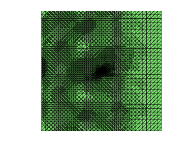
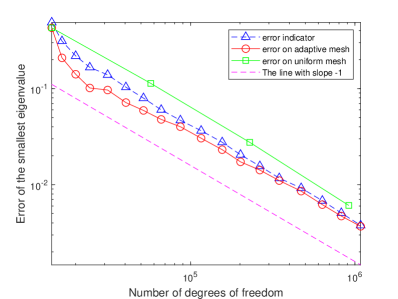
Figure 1: Adaptive mesh after $l$=7 refinement times (left) and error curves (right) of the smallest eigenvalue by DGFEM using $\mathbb{P}_{1}-\mathbb{P}_{0}$ element on $\Omega_{C}$.

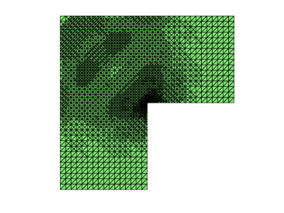
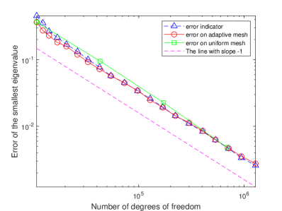
Figure 2: Adaptive mesh after $l$=7 refinement times (left) and the error curves (right) of the smallest eigenvalue by DGFEM using $\mathbb{P}_{1}-\mathbb{P}_{0}$ element on $\Omega_{L}$.

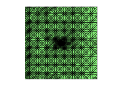
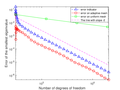
Figure 3: Adaptive mesh after $l$=15 refinement times (left) and the error curves (right) of the smallest eigenvalue by DGFEM using $\mathbb{P}_{2}-\mathbb{P}_{1}$ element on $\Omega_{C}$.

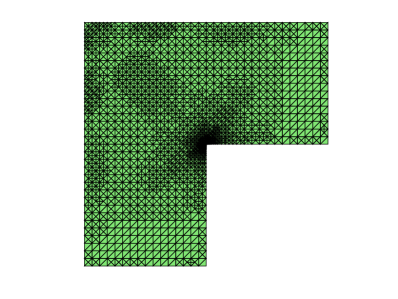
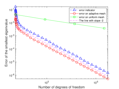
Figure 4: Adaptive mesh after $l$=15 refinement times (left) and error curves (right) of the smallest eigenvalue by DGFEM using $\mathbb{P}_{2}-\mathbb{P}_{1}$ element on $\Omega_{L}$.

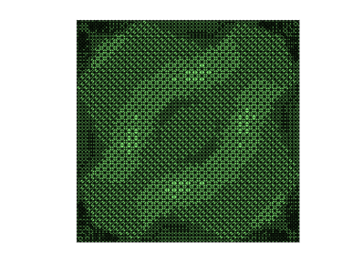
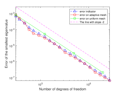
Figure 5: Adaptive mesh after $l$=7 refinement times (left) and the error curves (right) of the smallest eigenvalue by DGFEM using $\mathbb{P}_{2}-\mathbb{P}_{1}$ element on $\Omega_{S}$.

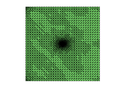
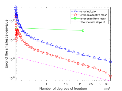
Figure 6: Adaptive mesh after $l$=25 refinement times (left) and the error curves (right) of the smallest eigenvalue by DGFEM using $\mathbb{P}_{3}-\mathbb{P}_{2}$ element on $\Omega_{C}$

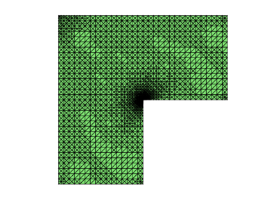
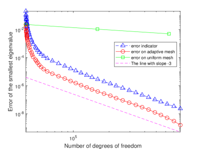
Figure 7: Adaptive mesh after $l$=25 refinement times (left) and the error curves (right) of the smallest eigenvalue by DGFEM using $\mathbb{P}_{3}-\mathbb{P}_{2}$ element on $\Omega_{L}$ .

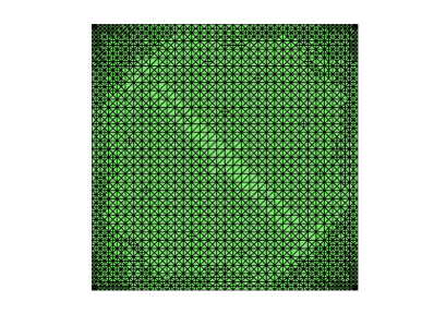
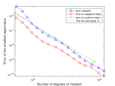
Figure 8: Adaptive mesh after $l$=5 refinement times (left) and the error curves (right) of the smallest eigenvalue by DGFEM using $\mathbb{P}_{3}-\mathbb{P}_{2}$ element on $\Omega_{S}$.

Table 1:  The smallest eigenvalue using $\mathbb{P}_{3}-\mathbb{P}_{2}$ element on adaptive mesh on $\Omega_{C}$.

$l$	$dof$	$\lambda_{1,h_{l}}$	$l$	$dof$	$\lambda_{1,h_{l}}$
1	53248	29.950023991	26	63206	29.916921865
2	53300	29.937640600	27	64610	29.916904165
5	53560	29.917626784	30	73424	29.916878484
10	54028	29.917180037	35	110630	29.916865373
11	54158	29.917248497	36	122876	29.916864735
14	54574	29.917406356	39	159094	29.916863538
15	54756	29.917731006	40	175812	29.916863378
21	57928	29.917153931	46	335842	29.916862940
22	58604	29.917092477	47	374920	29.916862915
23	59228	29.917021023	48	424814	29.916862902
24	60268	29.916986202	49	475852	29.916862889
25	61412	29.916940636	50	537862	29.916862882

Table 2:  The smallest eigenvalue using $\mathbb{P}_{3}-\mathbb{P}_{2}$ element on adaptive mesh on $\Omega_{L}$.

$l$	$dof$	$\lambda_{1,h_{l}}$	$l$	$dof$	$\lambda_{1,h_{l}}$
1	39936	32.155997914	27	53612	32.132716405
2	39988	32.148565928	28	56420	32.132709908
3	40092	32.147074075	29	60424	32.132705093
4	40196	32.141536961	30	66664	32.132701814
5	40248	32.139031080	31	75140	32.132699385
13	40924	32.134988686	39	181662	32.132694920
14	41080	32.134620945	40	205244	32.132694843
15	41288	32.134171324	41	229424	32.132694780
23	48048	32.132766985	49	616304	32.132694655
24	48880	32.132752576	50	703092	32.132694653
25	50128	32.132737367	51	796276	32.132694652
26	51688	32.132725042

Table 3:  The smallest eigenvalue using $\mathbb{P}_{3}-\mathbb{P}_{2}$ element on adaptive mesh on $\Omega_{S}$.

$l$	$dof$	$\lambda_{1,h_{l}}$	$l$	$dof$	$\lambda_{1,h_{l}}$
1	53248	52.3446926681	10	273780	52.3446911721
2	55900	52.3446918954	11	337324	52.3446911702
3	68952	52.3446915184	12	415636	52.3446911691
4	81588	52.3446913292	13	505544	52.3446911686
5	95316	52.3446912380	14	610376	52.3446911684
6	114192	52.3446912049	15	768560	52.3446911683
7	138372	52.3446911859	16	972192	52.3446911681
8	170612	52.3446911794	17	1186328	52.3446911679
9	220324	52.3446911751

4.2 The results in three-dimensional domains

We also carry out numerical experiments on two three-dimensional domains: $\Omega_{1}=(0,1)^{3}\setminus\{0\leq x\leq 0.5,0\leq y\leq 0.5,0.5\leq z\leq 1\}$ and $\Omega_{2}=(0,1)^{3}$. In computation we take $\theta=0.25$ and initial mesh $\pi_{h_{0}}$ ($h_{0}=\frac{\sqrt{3}}{8}$ ). To compute the error of the first eigenvalue for the Stokes eigenvalue problem, we choose the values $\lambda_{1}=70.98560$ and $62.17341$ which are obtained by adaptive procedure with as much degrees of freedom as possible as the reference values for the domains $\Omega_{1}$ and $\Omega_{2}$, respectively.                                
The initial meshes are shown in Figures 9-11, and the adaptive refined meshes and the error curves are shown in Figures 12-17. The numerical results on adaptive mesh are listed in Tables 1-3.
From Figures 12-17 we can see that the error curves and error indicators curves for DG methods using $\mathbb{P}_{k}-\mathbb{P}_{k-1}$ $(k=1,2,3)$ element are both approximately parallel to the line with slope $-\frac{2k}{3}$ , which indicates the error indicators are reliable and efficient and the adaptive algorithm can reach the optimal convergence order. It coincides with our theoretical analysis. It also can be seen from the error curves that under the same $dof$, the approximations obtained by high order elements are more accurate than those computed by low order elements on both uniform meshes and adaptive meshes.
We can also see from Table 2 that it provides an upper bound for the exact eigenvalue by $\mathbb{P}_{k}-\mathbb{P}_{k-1}$ element. Note that the numerical results in Table 5 in [55] provide a lower bound on the cubic domain by the CR element. Thus we get a range for the exact eigenvalue of Stokes eigenvalue problem on the cubic.

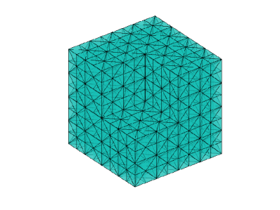
Figure 9: The initial mesh on $\Omega_{1}$(left) and $~{}\Omega_{2}$(right).

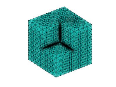
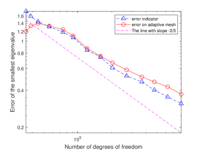
Figure 10: Adaptive mesh after $l$=10 refinement times (left) and the error curves (right) of the smallest eigenvalue by DGFEM using $\mathbb{P}_{1}-\mathbb{P}_{0}$ element on $\Omega_{1}$

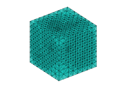
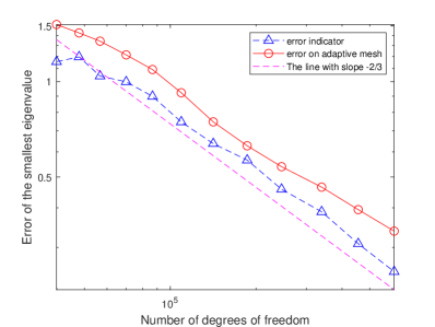
Figure 11: Adaptive mesh after $l$=10 refinement times (left) and the error curves (right) of the smallest eigenvalue by DGFEM using $\mathbb{P}_{1}-\mathbb{P}_{0}$ element on $\Omega_{2}$

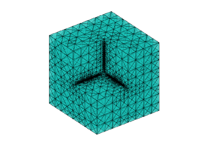
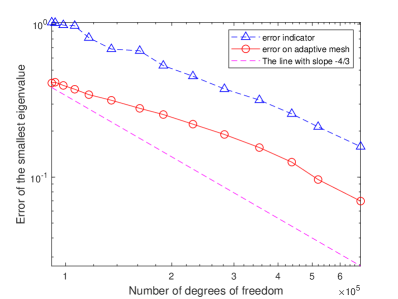
Figure 12: Adaptive mesh after $l$=14 refinement times (left) and the error curves (right) of the smallest eigenvalue by DGFEM using $\mathbb{P}_{2}-\mathbb{P}_{1}$ element on $\Omega_{1}$

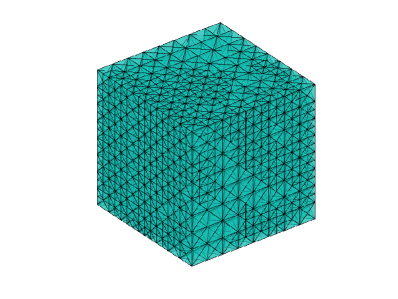
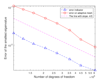
Figure 13: Adaptive mesh after $l$=8 refinement times (left) and the error curves (right) of the smallest eigenvalue by DGFEM using $\mathbb{P}_{2}-\mathbb{P}_{1}$ element on $\Omega_{2}$

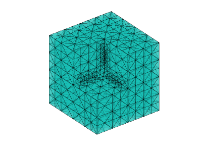
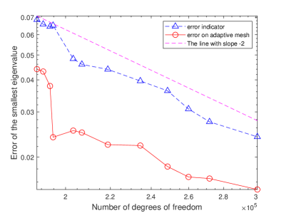
Figure 14: Adaptive mesh after $l$=12 refinement times (left) and the error curves (right) of the smallest eigenvalue by DGFEM using $\mathbb{P}_{3}-\mathbb{P}_{2}$ element on $\Omega_{1}$

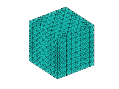
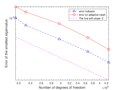
Figure 15: Adaptive mesh after $l$=5 refinement times (left) and the error curves (right) of the smallest eigenvalue by DGFEM using $\mathbb{P}_{3}-\mathbb{P}_{2}$ element on $\Omega_{2}$

Table 4:  The smallest eigenvalue on adaptive mesh on $\Omega_{1}$.

		$\mathbb{P}_{1}-\mathbb{P}_{0}$		$\mathbb{P}_{2}-\mathbb{P}_{1}$		$\mathbb{P}_{3}-\mathbb{P}_{2}$
$l$	$dof$	$\lambda_{1,h_{l}}$	$dof$	$\lambda_{1,h_{l}}$	$dof$	$\lambda_{1,h_{l}}$
1	34944	72.17893	91392	71.39751	188160	70.94156
2	38532	72.31180	93432	71.40261	190680	70.94249
3	44668	72.37533	98532	71.38286	193480	70.94775
4	56108	72.30857	106148	71.36073	194740	70.96169
5	74074	72.22436	116416	71.33137	203280	70.96023
6	91416	72.08199	134844	71.30330	207060	70.96067
7	121212	71.85217	162248	71.26700	218820	70.96323
8	159224	71.73561	189244	71.24186	234500	70.96341
9	202878	71.64715	229568	71.20735	248500	70.96722
10	270738	71.56537	281928	71.17551	259840	70.96886
11	369278	71.49289	354212	71.14148	271740	70.96910
12	475852	71.44762	437512	71.11079	300860	70.97064
13	623792	71.40660	519588	71.08194	412653	70.98560
14	822172	71.35097	685780	71.05522	-	-

Table 5:  The smallest eigenvalue on adaptive mesh on $\Omega_{2}$.

		$\mathbb{P}_{1}-\mathbb{P}_{0}$		$\mathbb{P}_{2}-\mathbb{P}_{1}$		$\mathbb{P}_{3}-\mathbb{P}_{2}$
l	$dof$	$\lambda_{1,h_{l}}$	$dof$	$\lambda_{1,h_{l}}$	$dof$	$\lambda_{1,h_{l}}$
1	39936	63.68761	104448	62.28426	215040	62.17483
2	47892	63.59785	128520	62.26349	231840	62.17461
3	56732	63.51520	160820	62.24599	296800	62.17423
4	70044	63.38799	207944	62.22633	366520	62.17393
5	86632	63.26514	267920	62.21249	427560	62.17376
6	109252	63.09579	352648	62.19957	491060	62.17341
7	141440	62.91980	448664	62.18869	-	-
8	186004	62.80083	611864	62.18345	-	-
9	245440	62.71246	-	-	-	-
10	339248	62.63796	-	-	-	-
11	455754	62.56792	-	-	-	-
12	608998	62.51093	-	-	-	-

References

- [1] I. Babuska, W. C. Rheinboldt, Error estimates for adaptive finite element computations, SIAM .J. Numer. Anal. vol. 15 (1978)pp. 736-754.
- [2] R. Verfrth, A Posteriori Error Estimation Techniques, Oxford University Press, New York, 1996.
- [3] W. Dorfler, A convergent adaptive algorithm for Poisson’s equation, SIAM J. Numer. Anal. vol. 33 (1996) pp. 1106-1124.
- [4] P. Morin, R. H. Nochetto, K. Siebert, Convergence of adaptive finite element methods, SIAM Rev. vol. 44 (2002)pp. 631-658.
- [5] M. Ainsworth, J. T. Oden, A Posteriori Error Estimation in Finite Element Analysis, Wiley-Interscience, New York, 2011.
- [6] S.C. Brenner, interior penalty methods, In Frontiers in Numerical Analysis-Durham 2010, Lecture Notes in Computational Science and Engineering, Springer-Verlag, vol. 85 (2012)pp. 79-147.
- [7] Z. Shi, M. Wang, Finite Element Methods, Scientific Publishers, Beijing, 2013.
- [8] J. Sun, A. Zhou, Finite Element Methods for Eigenvalue Problems, CRC Press, Taylor Francis Group, Boca Raton, London, New York, 2016.
- [9] C. Lovadina, M. Lyly, Stenberg, R.: A posteriori estimates for the Stokes eigenvalue problem. Numer. Methods Partial Differ. Equ. vol. 25 (1) (2009)pp. 244-257.
- [10] J. Han, Z. Zhang, Y. Yang, A new adaptive mixed finite element method based on residual type a posterior error estimates for the Stokes eigenvalue problem. Numer. Methods Partial Differ. Equ. vol. 31 (1) (2015)pp. 31-53.
- [11] M. G. Armentano, V. Moreno, A posteriori error estimates of stabilized low-order mixed finite elements for the Stokes eigenvalue problem, J. Comput. Appl. Math. vol. 269 (2014)pp. 132-149.
- [12] H. Liu, W. Gong, S. Wang, N. Yan, Superconvergence and a posteriori error estimates for the Stokes eigenvalue problems. BIT. vol. 53 (3) (2013)pp. 665-687.
- [13] S. Jia, F. Lu, H. Xie, A Posterior error analysis for the nonconforming discretization of Stokes eigenvalue problem. Acta Mathematica Sinica (English Series), 2014.
- [14] J. Gedicke, A. Khan, Arnold-Winther mixed finite elements for Stokes eigenvalue problems. SIAM J. Sci. Comput. vol. 40 (5) (2018)pp. A3449-A3469.
- [15] nder, Trk, Daniele, Ramon Codina. A stabilized finite element method for the two-field and three-field Stokes eigenvalue problems. Comput. Methods Appl. Mech. Engrg. 310 (2016) 886-905
- [16] W. H. Reed and T. R. Hill, Triangular mesh methods for the neutron transport equation, Technical Report LA-UR-73-479, Los Alamos Scientifik Laboratory, 1973.
- [17] B.Cockburn, G.E.Karniadakis, C. Shu, Discontinuous Galerkin Methods,Thoery, Computation and Applications, Springer-Verlag, 1999.
- [18] Jan S. Hesthaven, Tim Warburton, Nodal Discontinuous Galerkin Methods, Algorithms, Analysis, and Applications. Springer-Verlag, New York, 2008.
- [19] B. Rivire, Discontinuous Galerkin Methods for Solving Elliptic and Parabolic Equations. Theory and Implementation, SIAM. 2008.
- [20] D.A. Di Pietro and A. Ern, Discrete functional analysis tools for discontinuous Galerkin methods with application to the incompressible Navier-Stokes equations, Math. Camp. vol 79(271) (2010) pp.1303-1330.
- [21] A.Cangianl, Z.Dong, E.H.Georgoulis, P.Houston, hp-Version Discontinuous Galerkin Method on Polygonal and Polyhedral Meshes, Springer, 2010.
- [22] D. Antonio, E. Alexandre, Mathematical Aspects of Discntinuous Galerkin Methods, Springer-Verlag, 2012.
- [23] A. Ern, L J Ond Rm Gue, Finite Elements IIGalerkin approximation, elliptic and mixed PDEs. 2021.
- [24] F. Brezzi, G. Manzini, D. Marini, P. Pietra, A. Russo, Discontinuous Galerkin approximations for elliptic problems. Numer. Methods Partial Differ. Equ. 16 (4) (2000)pp. 365-378.
- [25] P. F. Antonietti, A. Buffa, I. Perugia, Discontinuous Galerkin approximation of the Laplace eigenproblem. Comput. Meth. Appl. Mech. Engrg. vol. 195 (25/28) (2006)pp. 3483-3503.
- [26] Y. Zeng, F. Wang, A posteriori error estimates for a discontinuous Galerkin approximation of Steklov eigenvalue problems. Appl. Math. vol. 62 (3) (2017)pp. 243-267.
- [27] S. C. Brenner, P. Monk, J. Sun, interior penalty Galerkin method for biharmonic eigenvalue problems. Spectral and High Order Methods for Partial Differential Equations, Lect. Notes Comput. Sci. Eng. 106 (2015) pp.3-15.
- [28] L. Wang, C. Xiong, H. Wu, F. Luo, A priori and a posteriori analysis for discontinuous Galerkin finite element approximations of biharmonic eigenvalue problems, Adv. Comput. Math. 45(5-6) (2019) pp. 2623-2646.
- [29] H. Geng, X. Ji, J. Sun, L. Xu, IP methods for the transmission eigenvalue problem, J. Sci, Comput. 68(2016) pp.326-338.
- [30] Y. Yang, H. Bi, H. Li, J. Han, A IPG method and its error estimates for the Helmholtz transmission eigenvalue problem, J. Comput. Appl. Math. vol. 326 (2017)pp. 71-86.
- [31] A. Buffa, I. Perugia, Discontinuous Galerkin approximation of the Maxwell eigenproblem, SIAM J. Numer. Anal. vol. 44(5) (2006)pp. 2198-2226.
- [32] A. Buffa, P. Houston, I. Perugia, Discontinuous Galerkin computation of the Maxwell eigenvalues on simplicial meshes, J. Comput. Appl. Math. vol. 204 (2007)pp. 317-333.
- [33] J. Gedicke , A. Khan , Divergence-conforming discontinuous Galerkin finite elements for Stokes eigenvalue problems, Numer. Math. 144 (3) (2019)pp. 585-611.
- [34] F. Lepea, Mora D . Symmetric and Nonsymmetric Discontinuous Galerkin Methods for a Pseudostress Formulation of the Stokes Spectral Problem. SIAM Journal on Scientific Computing, 42 (2) (2020)pp. A698-A722.
- [35] S. Badia, et al., Error analysis of discontinuous Galerkin methods for the Stokes problem under minimal regularity. IMA. J. Numer. Anal. vol. 34(2014)pp. 800-819.
- [36] P. Hansbo and M. G. Larson, Discontinuous Galerkin methods for incompressible and nearly incompressible elasticity by Nitsche’s method, Comput. Methods Appl. Mech. Engrg. vol. 191 (2002)pp. 1895-1908.
- [37] V. Girault, B. Rivie‘re, M.F. Wheeler, A discontinuous Galerkin method with non-overlapping domain decomposition for the Stokes and Navier-Stokes problems, Math. Comput. vol. 74 (2005)pp. 53-84.
- [38] B. Rivire and V. Girault, Discontinuous finite element methods for incompressible flows on subdomains with non-matching interfaces, Computer Methods in Applied Mechanics and Engineering, 195 (25/28) (2006) 3274-3292.
- [39] A. Toselli, hp discontinuous Galerkin approximations for the Stokes problem, Math. Models Methods Appl. Sci. vol. 12 (11) (2002)pp. 1565-1597
- [40] P. Houston, D. Schtzau, T.P. Wihler, Energy norm a posteriori error estimation for mixed discontinuous Galerkin approximations of the Stokes problem. J. Sci. Comput. vol. 22 (23) (2005)pp. 347-370.
- [41] O. A. Karakashian, F. Pascal, A posteriori error estimates for a discontinuous Galerkin approximation of second-order elliptic problems. SIAM J. Numer. Anal. vol. 41(6)(2004) pp. 2374-2399.
- [42] S.C. Brenner, Poincaré-Friedrichs inequalities for piecewise functions. SIAM J. Numer. Anal. vol. 41 (2003)pp. 306-324.
- [43] D. Schtzau, C. Schwab, A. Toselli, Mixed hp-DGFEM for incompressible flows. SIAM J. Numer. Anal. vol. 40 (6) (2002)pp. 2171-2194.
- [44] I. Perugia, D. Schtzau, The -local discontinuous Galerkin method for low-frequency time-harmonic Maxwell equations. Math. Comp. vol. 72 (2002)pp. 1179-1214.
- [45] P. Houston, I. Perugia, D. Schtzau. An a posteriori error indicator for discontinuous Galerkin discretizations of H(curl)-elliptic partial differential equations. IMA J. Numer. Anal. vol. 27 (2007)pp. 122-150.
- [46] I. Babuska, J.E. Osborn, Eigenvalue problems, in: P.G. Ciarlet, J.L. Lions (Eds.), Finite Element Methods (Part I), in: Handbook of Numerical Analysis, vol.2, North-Holland: Elsevier Science Publishers, (1991)pp. 641-787.
- [47] D. Boffi, Finite element approximation of eigenvalue problems, Acta Numer. vol. 19 (2010)pp. 1-120.
- [48] Y.Yang, Z. Zhang, F. Lin: Eigenvalue approximation from below using non-conforming finite elements. Sci. China, Math. vol. 53 (2010)pp. 137-150.
- [49] L. R. Scott, S. Zhang, Finite element interpolation of non-smooth functions satisfying boundary conditions, Math. Comp. vol. 54 (1990)pp. 483-493.
- [50] G. Kanschat, D. Schtzau. Energy norm a posteriori error estimation for divergence-free discontinuous Galerkin approximations of the Navier-Stokes equations. Int. J. Numer. Meth. in Fluids, 2008.
- [51] H. Wu, Z. Zhang, Can we have superconvergent gradient recovery under adaptive meshes, SIAM J. Numer. Anal. vol. 45 (2007)pp. 1701-1722.
- [52] Y. Yang, Y. Zhang, H. Bi, A type of adaptive non-conforming finite element method for the Helmholtz transmission eigenvalue problem, Comput. Methods Appl. Mech. Engrg, 360 (2020), Doi: 10.1016/j.cma.2019.112697.
- [53] X. Dai, J. Xu, A. Zhou, Convergence and optimal complexity of adaptive finite element eigenvalue computations, Numer. Math. vol. 110 (2008)pp. 313-355.
- [54] L. Chen, iFEM: An integrated finite element method package in matlab, Technical Report, University of California at Irvine, 2009.
- [55] L. Sun, Y. Yang, The a posteriori error estimates and adaptive computation of nonconforming mixed finite elements for the Stokes eigenvalue problem, Applied Mathematics and Computation, 421 (2022) 126951.
- [56] F. Lepe, G. Rivera, A virtual element approximation for the pseudostress formulation of the Stokes eigenvalue problem, Comput. Methods Appl. Mech. Engrg. 379 (2021) 113753.
- [57] V. Girault, P.A. Raviart, Finite Element Approximation of the Navier-Stockes Equations. Springer-Verlag, 1979.
- [58] B. Rivire and V. Girault, Discontinuous finite element methods for incompressible flows on subdomains with non-matching interfaces, Comput. Meth. Appl. Mech. Engrg. vol. 195(2006)pp. 3274-3292.