Independent Learning in Mean-Field Games: Satisficing Paths and Convergence to Subjective Equilibria

Abstract

Independent learners are agents that employ single-agent algorithms in multi-agent systems, intentionally ignoring the effect of other strategic agents. This paper studies mean-field games from a decentralized learning perspective, with two primary objectives: (i) to identify structure that can guide algorithm design, and (ii) to understand the emergent behaviour in systems of independent learners. We study a new model of partially observed mean-field games with finitely many players, local action observability, and a general observation channel for partial observations of the global state. Specific observation channels considered include (a) global observability, (b) local and mean-field observability, (c) local and compressed mean-field observability, and (d) only local observability. We establish conditions under which the control problem of a given agent is equivalent to a fully observed MDP, as well as conditions under which the control problem is equivalent only to a POMDP. Building on the connection to MDPs, we prove the existence of perfect equilibrium among memoryless stationary policies under mean-field observability. Leveraging the connection to POMDPs, we prove convergence of learning iterates obtained by independent learning agents under any of the aforementioned observation channels. We interpret the limiting values as subjective value functions, which an agent believes to be relevant to its control problem. These subjective value functions are then used to propose subjective Q-equilibrium, a new solution concept for partially observed n-player mean-field games, whose existence is proved under mean-field or global observability. We provide a decentralized independent learning algorithm for partially observed n-player mean-field games, and we show that it drives play to subjective Q-equilibrium by adapting the recently developed theory of satisficing paths to allow for subjectivity. Our algorithm is decentralized, in that it uses only local information for learning and allows players to use different, heterogenous policies during play. As such, it departs from the conventional representative agent approach common to other algorithms for mean-field games.

Keywords: Multi-agent reinforcement learning, independent learners, learning in games, mean-field games, decentralized systems

1 Introduction

Mean-field games are a theoretical framework for studying strategic environments with a large number of weakly coupled decision-making agents Huang et al. (2006, 2007); Lasry and Lions (2007). In a mean-field game, the cost and state dynamics of any particular agent are influenced by the collective behaviour of others only through a distributional mean-field term. Due to the ubiquity of large-scale decentralized systems in modern engineering, mean-field games have been used to model a diverse range of applications, such as resource management (e.g. Guéant et al. (2011) and Bauso et al. (2012)), social conventions Gomes et al. (2014), power control in telecommunications networks Yang et al. (2016), traffic control Chevalier et al. (2015), and opinion dynamics Stella et al. (2013) among many others.

Multi-agent reinforcement learning (MARL) is the study of the emergent behaviour in systems of interacting learning agents, with stochastic games serving as the most popular framework for modelling such systems Littman (1994); Zhang et al. (2021). In recent years, there has been a considerable amount of research in MARL that has aimed to produce algorithms with desirable system-wide performance and convergence properties. While these efforts have lead to a number of empirically successful algorithms, there are fewer works that offer formal convergence analyses of their algorithms, and the bulk of existing work is suitable only for systems with a small number of agents.

There are several competing paradigms for studying multi-agent learning. The Bayesian learning paradigm, popularized by Kalai and Lehrer (1993), studies agents who maintain beliefs on the policies used by other agents. Bayesian learners select policies to best-respond to their beliefs, while beliefs are updated as new information arrives during the course of play. In this framework, under certain conditions aligning the beliefs of agents with the actual policies used by other agents, several results on the convergence of play to (objective) equilibrium were proved. Despite its elegance and epistemic appeal, the Bayesian learning framework has two major shortcomings. First, the paradigm does not lend itself to tractable algorithms, as players must maintain beliefs over the strategies used by every other agent, and these strategies can be arbitrarily complex, history-dependent objects. The second shortcoming of Bayesian learning has to do with the restrictive conditions under which its results hold. We cite Nachbar (2005) as the most notable example of a negative result highlighting the limitations of Bayesian learning.

One desirable feature of the Bayesian framework is its explicit consideration of beliefs. Subjectivity and beliefs are relevant to MARL at large, as they allow for players to be uncertain of the model of the game being played, rather than allowing only for uncertainty in the policies of the other agents or unobservable hidden variables whose distributions are known. Kalai and Lehrer (1995) proposed a notion of subjective equilibrium for the Bayesian learning paradigm, in which players behave optimally with respect to their subjectively held beliefs and, furthermore, each player’s subjective beliefs satisfy a consistency condition with respect to the observed trajectory of play. Several other notions of subjective equilibrium have been proposed in the literature, some of which are structural and non-Bayesian, in that the agents believe a particular model to be true and act in accordance with their structural assumptions. We refer the reader to Arslan and Yüksel (2023) for a review. In this paper, we propose subjective Q-equilibrium, a new non-Bayesian notion of subjective equilibrium that we argue is well-suited to decentralized learning in large-scale systems, where agents suffer from a high degree of uncertainty and may need to make structural assumptions about their system for tractability. This equilibrium definition contributes to an emerging line of work that studies simple agents in complex, possibly non-Markovian environments with a perceived local state Dong et al. (2022); Chandak et al. (2022); Kara and Yüksel (2022, 2023). This will be discussed further later in the paper.

Outside of the Bayesian learning paradigm, the majority of theoretical contributions in MARL have focused on highly structured classes of stochastic games, such as two-player zero-sum games Daskalakis et al. (2021); Sayin et al. (2021, 2022) and $n$-player stochastic teams and their generalizations (Arslan and Yüksel (2017), Ding et al. (2022); Fox et al. (2022); Leonardos et al. (2021); Mguni et al. (2021); Unlu and Sayin (2023), Yongacoglu et al. (2022), Zhang et al. (2022)). In much of the existing literature on MARL, a great deal of information is assumed to be available to agents while they learn. These assumptions, such as full state observability (as assumed by Daskalakis et al. (2021) and Yongacoglu et al. (2022) among others) or action-sharing among all agents (as assumed by Littman and Szepesvári (1996); Hu and Wellman (2003) and Littman (2001)), are appropriate in some settings but are unrealistic in many large-scale, decentralized systems.

One issue with designing MARL algorithms that use global information about the local states and actions of all players is that such algorithms do not scale with the number of players. The so-called curse of many agents is a widely cited challenge to MARL, wherein the computational burden at each agent grows exponentially in the number of agents Wang et al. (2020).

Independent learners Matignon et al. (2009, 2012) are a class of MARL algorithms that are characterized by intentional obliviousness to the strategic environment: independent learners ignore the presence of other players, effectively treating other players as part of the environment rather than as the non-stationary learning agents that they actually are. By naively running a single-agent reinforcement learning algorithm using only local information, independent learners are relieved of the burden of excessive information, which may lead to scalable algorithms for large-scale decentralized systems. However, additional care must be taken when designing independent learners, as direct application of single-agent reinforcement learning has had mixed success in small empirical studies: see, for instance, the works of Condon (1990); Tan (1993); Sen et al. (1994) and Claus and Boutilier (1998). Here, we offer a new perspective on independent learners by framing their obliviousness as a subjective structural belief on the system within which they exist. Accordingly, agents may act rationally with respect to their (possibly incorrect) subjective beliefs. Building on this interpretation, we propose a new notion of subjective equilibrium that is inspired by, and therefore well-suited to, the analysis of independent learners in decentralized MARL. Structural properties of such subjective equilibria, such as their (non-) existence and their comparison to traditional solution concepts, may explain why independent learners lead to stable outcomes in certain MARL applications and not others.

The Learning Setting

In this paper, we study independent learners in partially observed $n$-player mean-field games. This finite agent model is closely related to the model presented in Saldi et al. (2018), but allows for a variety of observation channels through which agents can observe non-local information. Decentralization and learning are primary focuses of this study, and we are interested in online algorithms that involve minimal coordination between agents after play begins. Some salient characteristics of our model are the following:

Limited View of the Global State: Using a single, unified model, we consider four alternative observation channels by which players observe non-local state information. These are described below in summary of the contributions of this paper.

Local Action Information: A given player does not know the policies used by the remaining players, and the player does not observe the actions generated by these policies.

Decentralized, Online Feedback: In this study, players to not have access to the model governing the system, nor do they have access to a simulator/oracle/generative model for sampling data in an arbitrary order, nor do they have access to offline data sets that can be used for training. Instead, we assume that players view only the stream of data encountered during play, which is not shared across agents.

Decentralized Training: This work does not belong to the paradigm of centralized training with decentralized execution, in which a global value function is learned during training and players select policies that can be implemented in a decentralized manner informed by this global quantity. Examples of studies using this paradigm include the works of Peng et al. (2017); Lowe et al. (2017) and Foerster et al. (2018).

Heterogenous Policies during Learning: Since agents learn using different local information encountered during play, we avoid the common requirement that all agents employ the same policy at any given time.

Contributions:

1. In Section 2, we propose a new model of partially observed $n$-player mean-field games. This model is suitable for the study of decentralized learning and is flexible enough to model various alternative observation channels. In particular, each agent observes its own local actions and partially observes the global state. We consider several observation channels, including (a) global state observability, (b) local state and mean-field observability (c) local state and compressed mean-field information, and (d) only local state observability.

2. In Section 3, we show that if the remaining players follow (memoryless) stationary policies, then an individual faces a stochastic control problem equivalent to a POMDP (Lemma 6). Moreover, under mean-field observability and a symmetry condition on the policies of other players, Theorem 8 asserts that the player’s control problem is equivalent to a fully observed MDP. We also show that the MDP equivalence does not hold in general when one relaxes either mean-field observability or symmetry of the policies of the remaining players. This non-equivalence to an MDP in general is an important distinction between the finite player model studied here and the limit model with infinitely many agents studied elsewhere. In Theorem 12, for the case of mean-field observability, we prove the existence of perfect equilibrium policies in the set of (memoryless) stationary policies. This result builds on Theorem 8, and is of independent theoretical interest, beyond its relevance to independent learners.

3. We study the learning iterates obtained by independent learners in a partially observed $n$-player mean-field game. In Theorem 13, we show that when each agent uses a (memoryless) stationary policy and naively runs single-agent value estimation algorithms (Algorithm 1), its learning iterates converge almost surely under mild conditions on the game. In Appendix B, we characterize these almost sure limits in terms of underlying, implied MDPs faced by the agents. We offer a new perspective on independent learning, interpreting it as a subjective model adopted by the learning agent. The limiting values of the agent’s learning iterates are then interpreted as subjective value functions, in analogy to objective value functions in single-agent MDPs. With this interpretation, we define subjective $\epsilon$-best-responding in Definition 15 and we use this to define subjective $\epsilon$-equilibrium (also called subjective Q-equilibrium) in Definition 16. In Lemma 17, we show that subjective $\epsilon$-equilibrium exists under mean-field observability.

4. We present Algorithm 3, a decentralized independent learning algorithm for partially observed $n$-player mean-field games. We use a modified theory of satisficing paths to show that Algorithm 3 drives play to subjective $\epsilon$-equilibrium under mean-field observability (Theorem 25). Analogous results for other observation channels can be found in Appendix I: Algorithmic convergence under global observability is presented in Theorem 57, while an algorithmic result for compressed observability is given in Theorem 58, under an additional assumption on subjective equilibrium.

Organization

In §1.1 and §1.2, we survey related literature. The formal model is presented in Section 2. In Section 3, we examine the close connection between partially observed $n$-player mean-field games and partially/fully observed Markov decision problems (POMDP/MDPs). We provide conditions under which a player in a mean-field game faces a fully observed MDP, as well as conditions under which the player faces only a POMDP. We leverage this connection to prove existence of stationary (objective) perfect equilibria under mean-field observability. Independent learners and subjectivity are discussed in Section 4, where we show the convergence of iterates under partial observability. We discuss the interpretation of the limiting quantities as subjective value functions, and use this to define subjective Q-equilibrium (also called subjective $\epsilon$-equilibrium). Existence of subjective $\epsilon$-equilibrium is proved under mean-field observability. Algorithmic results are given in Section 5. The section begins by describing win-stay, lose-shift algorithms, and studies one such algorithm with oracle access to subjective value functions. Oracle access is subsequently relaxed, and a full-scale, decentralized learning algorithm is presented in Algorithm 3. The convergence of these algorithms to subjective $\epsilon$-equilibrium is analyzed using the theory of (subjective) satisficing paths. Results of a simulation study are presented in Section 6. Additional discussion on observation channels is given in Section 7. The final section concludes. Proofs omitted from the body of the paper are available in the appendices, along with a description of POMDPs and MDPs. An additional result on objective $\epsilon$-equilibrium under local observability is presented in Appendix G.

Notation: We use ${\rm Pr}$ to denote a probability measure on some underlying probability space, with additional superscripts and subscripts as needed. For a finite set $S$, we let $\mathbb{R}^{S}$ denote the real vector space of dimension $|S|$ where vector components are indexed by elements of $S$. We let $0\in\mathbb{R}^{S}$ denote the zero vector of $\mathbb{R}^{S}$ and $1\in\mathbb{R}^{S}$ denote the vector in $\mathbb{R}^{S}$ for which each component is 1. For standard Borel sets $S,S^{\prime}$, we let $\Delta(S)$ denote the set of probability measures on $S$ with the Borel $\sigma$-algebra on $S$, and we let $\mathcal{P}(S^{\prime}|S)$ denote the set of transition kernels on $S^{\prime}$ given $S$. We use $Y\sim\mu$ to denote that the random variable $Y$ has distribution $\mu$. For an event $\{\cdot\}$, we let $\textbf{1}\{\cdot\}$ denote the indicator function of the event $\{\cdot\}$’s occurrence. If a probability distribution $\mu$ is a mixture of distributions $\mu_{1},\dots,\mu_{n}$ with mixture weights $p_{1},\dots,p_{n}$, we write $Y\sim\sum_{i=1}^{n}p_{i}\mu_{i}$. For $s\in S$, we use $\delta_{s}\in\Delta(S)$ to denote the Dirac measure centered at $s$.

1.1 Related Work

A number of research items attempt to approximate solution concepts for mean-field games using learning algorithms. By and large, these works approach learning in mean-field games by analyzing the single-agent problem for a representative agent in the limiting case as $n\to\infty$, and equilibrium is defined using a best-responding condition as well as a consistency condition; see, for instance, (Subramanian and Mahajan, 2019, Definition 2.1). The solution concepts sought in these works are inherently symmetric: at equilibrium, all agents use the same policy as the representative agent. As a result, such equilibria may be difficult to learn in decentralized learning settings, where agents will use heterogenous policies during the learning process. We now describe a representative sample of works in this centralized learning tradition, and we refer the reader to Laurière et al. (2022) for a survey.

Guo et al. (2019) study a model of mean-field games that allows for costs and state dynamics to depend also on the distribution of actions of other players. Under somewhat stringent assumptions of Lipschitz continuity, an existence and uniqueness of equilibrium result is given, and an algorithm is presented for learning such an equilibrium with the assistance of a generative model for sampling transitions and cost data.

Subramanian and Mahajan (2019) study stationary mean-field games, in which optimality and equilibrium are defined in terms of the limiting invariant distribution of the mean-field state. The authors present multiple notions of equilibrium and study two-timescale policy gradient methods in this setting, wherein a representative agent updates its policy to best-respond to its (estimated) environment on the fast timescale and updates its estimate for the mean-field flow on the slow timescale. By assuming access to a simulator for obtaining data, convergence to a local notion of equilibrium is proved.

Mean-field games with a finite time horizon and uncountable state and action spaces are considered by Elie et al. (2020). A fictitious play algorithm of sorts is proposed and analyzed, though the question of learning to best-respond is black-boxed. Mguni et al. (2018) also present an algorithm based on fictitious play and make connections to the field of potential games. Another fictitious play algorithm is proposed by Xie et al. (2021). Their algorithm, which in some ways parallels the algorithm of Subramanian and Mahajan (2019), iteratively updates both the policy and the mean-field term at every step of its execution.

Anahtarcı et al. (2020) present a value iteration algorithm for computing stationary mean-field equilibrium in both discounted and average-cost mean-field games. The same authors extend and expand on this work in Anahtarci et al. (2023a), where they present results on the approximation of Nash equilibrium in the $n$-person game by mean-field equilibrium in the limiting regime. In a separate line of research, Anahtarci et al. (2023b) study regularized mean-field games and propose a learning algorithm based on fitted Q-learning. Algorithms and operators based on regularization are also studied by Cui and Koeppl (2021). Zaman et al. (2023a) present a two-timescale reinforcement learning algorithm that approximates stationary mean-field equilibrium, building on some analytical results presented in Cui and Koeppl (2021). The work of Zaman et al. (2023a) is closely related to that of Angiuli et al. (2022), which also presents a two-timescale algorithm.

An important special case of mean-field games, with linear state dynamics and quadratic costs, has been studied by several authors including Fu et al. (2019); Zaman et al. (2020a, b); Angiuli et al. (2022) and Zaman et al. (2023b).

In many of the preceding works, the authors restrict their attention to Markov policies that depend only on local state observations, without dependence on the mean-field distribution. At least two research items have considered learning with a focus on population-dependent policies, which condition one’s action choice on both the local state and the mean-field distribution. In this vein, Perrin et al. (2022) study the existence of so-called master policies and propose a learning algorithm for its computation. Mishra et al. (2023) propose an algorithm for learning mean-field equilibrium in finite horizon games, building on the sequential decomposition of Vasal (2023) and the common information approach of Nayyar et al. (2013).

A common theme uniting the works cited above is that they are centralized methods for finding equilibrium in a mean-field game modelling a decentralized system. The use of a simulator for obtaining data allows these algorithms to sample data as if it were generated by a population of agents using symmetric policies at each step of the algorithm. As a result, the problems studied are single-agent rather than multi-agent in flavour, due to the lack of strategic interaction in the mean-field limit. The principal aim of these papers is to use learning techniques to compute a (near) equilibrium for the mean-field games they study. In contrast, a primary aim of this paper is to understand the patterns of behaviour that emerge when agents use reasonable (if limited) learning algorithms in a shared environment. Our focus, then, is less computational and more descriptive in nature.

In many realistic settings, agents may employ different learning algorithms for a variety of reasons (e.g. due to differing prior beliefs on the system). Moreover, since distinct agents observe distinct local observation histories and feed these local observation histories to their learning algorithms, distinct agents may use radically different policies over the course of learning. Work in the computational tradition largely avoids such learning dynamics, and therefore does not encounter plausible equilibrium policies consisting of various heterogenous policies used by a population of homogenous players. In this paper, we depart from the traditional approach of mandating all agents to follow the same policy during learning.

The learning environment studied by Yardim et al. (2023) is perhaps the closest to the one considered in this paper. Yardim et al. (2023) study a decentralized learning problem in an $n$-player symmetric anonymous game with local observability and propose a mirror descent algorithm. Unlike the papers described earlier, the $n$ agents are allowed to use heterogenous policies during the course of learning. Under Lipschitz continuity assumptions on various operators, the authors show convergence to equilibrium in the regularized game, which can then be used to approximate mean-field equilibrium in a manner that depends on the degree of regularization.

At a high level, the primary objective of the literature surveyed above is to provide algorithms for the approximation of conventional variants of mean-field equilibrium. These works consider a variety of models for system interaction, a variety of objective criteria and time horizons, and at least two major solution concepts (predominantly stationary mean-field equilibrium, but occasionally non-stationary mean-field Nash equilibrium). To facilitate the design of such algorithms, many of these works conduct structural analysis on mean-field games, typically in the limiting regime with infinitely many players, and exclusively under symmetry conditions mandating that the entire population uses the policy of the representative agent.

Like the aforementioned papers, this paper makes contributions on the structure and analysis of mean-field games, focusing on the case with finitely many players and obtaining clear insights both with and without symmetry in policies. This is illustrated by the results and examples in Section 3. On the other hand, unlike the papers surveyed above, the goal of this paper is not the approximation of mean-field equilibria per se. Instead, the goal here is to better understand the outcomes of decentralized learning processes in large-scale systems. Since players use heterogenous, asymmetric policies during the learning process and iteratively adjust their behaviour as new information arrives, we do not restrict ourselves to the symmetric solution concepts of mean-field equilibrium. In Section 4, we propose a novel solution concept that we argue is well-suited for the study of decentralized learners in mean-field games. In considering alternative solution concepts for mean-field games, this paper is also related to the works of Lee et al. (2021); Subramanian et al. (2022b); Muller et al. (2022) and Campi and Fischer (2022).

Lee et al. (2021) study mean-field games with strategic complementarities. In that paper, the authors propose a trembling hand equilibrium concept and supply multiple algorithms for approximating it. Subramanian et al. (2022b) present an alternative model for decentralized mean-field games that is similar in spirit to the models put forth in Section 2 of the present paper. The authors then propose a model of decentralized mean-field equilibrium that attempts to capture heterogenous policies while preserving the overall consistency-optimality form of conventional mean-field equilibrium. Muller et al. (2022) propose mean-field correlated equilibrium and mean-field coarse correlated equilibrium, and show that, when compared to mean-field (Nash) equilibrium, these solution concepts can be learned under weaker assumptions on the game. In a related work, Campi and Fischer (2022) present and study a solution concept called the correlated solution of a mean-field game.

1.2 Applications of Mean-Field Games

We now describe a number of recent applications of mean-field games. This section is intended to serve as a sampling of the applied literature, rather than a comprehensive overview. For a survey of some classical applications of mean-field games, see Gomes and Saúde (2014).

Xia et al. (2019) study peer-to-peer energy markets in an electrical grid, in which agents act as producers and consumers at different times. The problem is modelled as a mean-field game with local observability, in which states are budgets. Consumers are paired with producers according to an external matching system, and they interact by exchanging bids for service provision. The mean-field quality of the application owes to the large population size and the random matching of consumers and producers, according to which a player’s best response depends on the distribution of other agents’ budgets.

Li et al. (2019) consider vehicle dispatch in a ride-sharing application from the driver’s perspective. The authors model the problem as an instance of independent learning in a mean-field game. The approach used there is philosophically well-aligned with the present paper: players observe an aggregate environmental state (describing weather conditions, traffic congestion, and so on) as well as local information about rides in their vicinity, and use this information to guide their action choice. The authors rule out the use of global Q-functions and algorithmic methods that track global data, and instead propose an independent MARL algorithm based on Q-learning. The method proposed by Li et al. (2019) results in the manipulation of an object resembling a Q-function: for agent $i$, they consider a quantity denoted $Q_{i}(o_{i},a_{i})$, which attempts to assign a value to playing action $a_{i}$ after observing the symbol $o_{i}$. Strictly speaking, this object is not a Q-function, since the agent does not face an MDP. Nevertheless, the authors observe that this approach leads to tractable, decentralized algorithms that outperform their centralized predecessors.

In addition to ride-dispatching, traffic routing in general is often modelled as a mean-field game, where overall travel time depends on the distribution of agents through the traffic network. Salhab et al. (2018) consider an instance of traffic routing as a mean-field game with mean-field observability, where availability of the mean-field is justified through the use of a mobile application. In a related study, Cabannes et al. (2021) model traffic routing as a mean-field game with local observability, where an agent’s local state is its location in the road network, its waiting time, and its destination node in the graph.

Resource allocation and management constitutes another major application of mean-field games, where a large number of agents compete for resources, often through auctions. Examples of applied work in this line includes service in a cellular network Manjrekar et al. (2019), auctions for advertisements Iyer et al. (2014), resource distribution in smart grids Li et al. (2018) and device-to-device wireless transmission Li et al. (2016).

2 Model

In this section, we present our model of partially observed $n$-player mean-field games, where several strategic agents interact in a shared environment. In subsequent sections, we will investigate the deep connection between our model of mean-field games and the single-agent model of partially observed Markov decision problems (POMDPs). Background material on POMDPs and fully observed MDPs can be found in Appendix A.

2.1 Partially Observed Mean-Field Games

For $n\in\mathbb{N}$, a partially observed $n$-player mean-field game is described by a list G:

$$\textnormal{{G}}=(\mathcal{N},\mathbb{X},\mathbb{Y},\mathbb{A},\{\varphi^{i}\}_{i\in\mathcal{N}},c,\gamma,P_{{\rm loc}},\nu_{0}).$$ (1)

The game G consists of $n$ players/agents, indexed by $\mathcal{N}=\{1,\dots,n\}$. At time $t\in\mathbb{Z}_{\geq 0}$, the local state for player $i\in\mathcal{N}$ is denoted by $x^{i}_{t}\in\mathbb{X}$, where $\mathbb{X}$ is a finite set of local states. We let $\textnormal{{X}}:=\times_{i\in\mathcal{N}}\mathbb{X}$ denote the $n$-fold cartesian product of $\mathbb{X}$, indexed by $\mathcal{N}$. An element of X is called a global state, and the global state at time $t$ is denoted by $\textnormal{{x}}_{t}=(x^{i}_{t})_{i\in\mathcal{N}}$. The mean-field associated with global state $\textnormal{{x}}_{t}$ is denoted by $\mu_{t}\in\Delta(\mathbb{X})$ and defined as the empirical measure of $\textnormal{{x}}_{t}$:

$$\mu_{t}(B):=\frac{1}{n}\sum_{i\in\mathcal{N}}\delta_{x^{i}_{t}}(B),\quad\forall B\subseteq\mathbb{X}.$$

Each player $i\in\mathcal{N}$ observes the global state $\textnormal{{x}}_{t}$ indirectly, making the local observation $y^{i}_{t}=\varphi^{i}(\textnormal{{x}}_{t})$, where $\mathbb{Y}$ is a finite set and $\varphi^{i}:\textnormal{{X}}\to\mathbb{Y}$ is player $i$’s observation function. Each player $i$ uses its locally observable history variable $h^{i}_{t}\in H_{t}$, to be defined shortly, to select an action $a^{i}_{t}\in\mathbb{A}$, where $\mathbb{A}$ is a finite set of actions. We denote the joint action of all players by $\textnormal{{a}}_{t}=(a^{i}_{t})_{i\in\mathcal{N}}$, and note that player $i$ only observes its own action $a^{i}_{t}$. After choosing action $a^{i}_{t}$, player $i$ incurs a stage cost of $c^{i}_{t}=c(x^{i}_{t},\mu_{t},a^{i}_{t})$, where $c:\mathbb{X}\times\Delta(\mathbb{X})\times\mathbb{A}\to\mathbb{R}$. Player $i$’s local state then evolves according to $x^{i}_{t+1}\sim P_{{\rm loc}}(\cdot|x^{i}_{t},\mu_{t},a^{i}_{t})$, where $P_{{\rm loc}}\in\mathcal{P}(\mathbb{X}|\mathbb{X}\times\Delta(\mathbb{X})\times\mathbb{A})$. Each player discounts its stream of costs using discount factor $\gamma\in(0,1)$, and the initial global state $\textnormal{{x}}_{0}$ has distribution $\nu_{0}$. The process repeats at time $t+1$ and so on.

Observation Channels and Local Information

In what follows, we refer to the pair $(\mathbb{Y},\{\varphi^{i}\}_{i\in\mathcal{N}})$ as the observation channel for the game G. To simplify the statement of assumptions on the observation channel, we define a function $\upmu:\textnormal{{X}}\to\Delta(\mathbb{X})$ that maps a global state to its empirical distribution:

$$\left(\upmu(\textnormal{{s}})\right)\left(B\right):=\frac{1}{n}\sum_{i\in\mathcal{N}}\delta_{s^{i}}(B),\quad B\subseteq\mathbb{X}.$$

With this notation, we have the mean-field state $\mu_{t}=\upmu(\textnormal{{x}}_{t})$ in the description of play above. We also define a finite subset ${\rm Emp}_{n}\subset\Delta(\mathbb{X})$ as ${\rm Emp}_{n}:=\{\upmu(\textnormal{{s}}):\textnormal{{s}}\in\textnormal{{X}}\}$.

In order to cover a diverse range of large, decentralized learning environments with a unified model, we now state some alternative observation channels that may be assumed.

Assumption 1 (Global Observability)

$\mathbb{Y}=\textnormal{{X}}$ and $\varphi^{i}(\textnormal{{s}})=\textnormal{{s}}$ for each global state $\textnormal{{s}}\in\textnormal{{X}}$ and player $i\in\mathcal{N}$.

Assumption 2 (Mean-Field Observability)

$\mathbb{Y}=\mathbb{X}\times{\rm Emp}_{n}$ and $\varphi^{i}(\textnormal{{s}})=(s^{i},\upmu(\textnormal{{s}}))$ for each global state $\textnormal{{s}}\in\textnormal{{X}}$ and player $i\in\mathcal{N}$.

Assumption 3 (Compressed Observability)

For $k\in\mathbb{N}$, let $[k]:=\{1,2,\dots,k\}$ and let $f:\Delta(\mathbb{X})\to[k]$. Then, $\mathbb{Y}=\mathbb{X}\times[k]$ and for each $i\in\mathcal{N}$, $\textnormal{{s}}\in\textnormal{{X}}$, we have $\varphi^{i}(\textnormal{{s}})=(s^{i},f(\upmu(\textnormal{{s}})).$

Assumption 4 (Local Observability)

$\mathbb{Y}=\mathbb{X}$ and $\varphi^{i}(\textnormal{{s}})=s^{i}$ for each $i\in\mathcal{N},\textnormal{{s}}\in\textnormal{{X}}$.

Assumptions 1–4 are presented in order of increasing decentralization. In practice, the particular choice of informational assumption will depend on one’s application area: in some instances, there will be a natural restriction of information leading to a particular observation channel. In other instances, agents may voluntarily compress a more informative observation variable for the purposes of function approximation. We now briefly describe these alternative observation channel assumptions. Additional discussion on this topic in Section 7.

In large-scale, decentralized systems, global observability is often unreasonable, but this case is included in our discussion as it is helpful for developing insights. This observational assumption appears in some works on linear-quadratic mean-field games, such as Zaman et al. (2020a, b). Mean-field observability is perhaps the most commonly considered observation channel in works on mean-field games. For examples of studies using mean-field observability, see Saldi et al. (2018), Zaman et al. (2023a) and the references therein. Local observability is also a commonly adopted assumption, see e.g. Muller et al. (2022); Yardim et al. (2023) and the references therein.

Compressed observability is an intermediate setting between mean-field and local observability. To our knowledge, this has not been explicitly considered in earlier work. Compressed observability can be motivated using the discussion above: it serves to lessen the computational burden at a given learning agent in a partially observed $n$-player mean-field game and, as we discuss in Section 7, may be a more appropriate modelling assumption in some applications. By taking $k=1$, we see that local state observability is in fact a special case of compressed state observability, where the compressed information about the mean-field state is uninformative. We include Assumption 4 separately to highlight the importance of this set-up.

Where possible, we conduct our analysis in a unified manner, without specifying the observation channel. In some instances, stronger results can be proved under richer observation channels. In such cases, our exposition and analysis centres on mean-field observability, with discussion on other information structures either omitted or postponed.

Local History Variables and Policies

We now formalize the action selection process by defining policies. We make distinctions between the overall system history and each player’s locally observable histories. For any $t\in\mathbb{Z}_{\geq 0}$, we define the sets

$$\textnormal{{H}}_{t} :=\left(\textnormal{{X}}\times\textnormal{{A}}\right)^{t}\times\textnormal{{X}},$$

$$H_{t} :=\Delta(\textnormal{{X}})\times\left(\mathbb{Y}\times\mathbb{A}\times\mathbb{R}\right)^{t}\times\mathbb{Y}.$$

For any $t\geq 0$, the set $\textnormal{{H}}_{t}$ represents the set of overall system histories of length $t$, while the set $H_{t}$ is the set of histories of length $t$ that an individual player in the game G may observe. Elements of $\textnormal{{H}}_{t}$ are called system histories of length $t$, and elements of $H_{t}$ are called observable histories of length $t$.

For each $t\geq 0$ and player $i\in\mathcal{N}$, we let

$$\textnormal{{h}}_{t} :=(\textnormal{{x}}_{0},\textnormal{{a}}_{0},\cdots,\textnormal{{x}}_{t-1},\textnormal{{a}}_{t-1},\textnormal{{x}}_{t}),$$

$$h^{i}_{t} :=(\nu_{0},y^{i}_{0},a^{i}_{0},c^{i}_{0},\cdots,y^{i}_{t-1},a^{i}_{t-1},c^{i}_{t-1},y^{i}_{t})$$

denote the $t^{\rm th}$ system history variable and player $i$’s $t^{\rm th}$ locally observable history variable, respectively. Note that $\textnormal{{h}}_{t}$ is a random quantity taking values in $\textnormal{{H}}_{t}$, while $h^{i}_{t}$ is a random quantity taking values in $H_{t}$.

Definition 1

A sequence $\pi^{i}=(\pi^{i}_{t})_{t\geq 0}$ with $\pi^{i}_{t}\in\mathcal{P}(\mathbb{A}|H_{t})$ for every $t\geq 0$ is called a policy for player $i$. We let $\Pi^{i}$ denote the set of all policies for player $i$.

Definition 2

A policy $\pi^{i}\in\Pi^{i}$ is called (memoryless) stationary (or simply stationary) if, for some $f^{i}\in\mathcal{P}(\mathbb{A}|\mathbb{Y})$, the following holds: for any $t\geq 0$ and any $\tilde{h}_{t}=(\nu,\tilde{y}_{0},\dots,\tilde{y}_{t})\in H_{t}$, we have $\pi^{i}_{t}(\cdot|\tilde{h}_{t})=f^{i}(\cdot|\tilde{y}_{t}).$ We let $\Pi^{i}_{S}$ denote the set of stationary policies for player $i$.

Remark: The set of policies—and therefore learning algorithms—available to an agent depends on the set of locally observable histories, which itself depends on the observation channel $(\mathbb{Y},\{\varphi^{i}\}_{i\in\mathcal{N}})$. In this paper, our focus is on independent learners, which are learners that do not use the joint action information in their learning algorithms. Here, we have chosen to incorporate this constraint into the information structure. Moreover, to underscore the importance of learning in our study, we also do not assume that the players know the cost function $c$. Instead, we assume only that they receive feedback costs in response to particular system interactions. These assumptions on the information structure resemble those of other work on independent learners, for example the works of Daskalakis et al. (2021); Sayin et al. (2021); Yongacoglu et al. (2022); Matignon et al. (2009, 2012); Wei and Luke (2016); Yongacoglu et al. (2023). A rather different information structure is that of joint action learners, as studied by Littman and Szepesvári (1996); Claus and Boutilier (1998); Hu and Wellman (2003) and Littman (2001), where the locally observable history variables also include the joint action history.

Notation: We let $\bm{\Pi}:=\times_{i\in\mathcal{N}}\Pi^{i}$ denote the set of joint policies. To isolate player $i$’s component in a particular joint policy $\bm{\pi}\in\bm{\Pi}$, we write $\bm{\pi}=(\pi^{i},\bm{\pi}^{-i})$, where $-i$ is used in the agent index to represent all agents other than $i$. Similarly, we write the joint policy set as $\bm{\Pi}=\Pi^{i}\times\bm{\Pi}^{-i}$, a joint action may be written as $\textnormal{{a}}=(a^{i},\textnormal{{a}}^{-i})\in\textnormal{{A}}:=\mathbb{A}^{\mathcal{N}}$, and so on.

Value Functions, Best-Responding, and Objective Equilibrium

For each player $i\in\mathcal{N}$, we identify the set of stationary policies $\Pi^{i}_{S}$ with the set $\mathcal{P}(\mathbb{A}|\mathbb{Y})$ of transition kernels on $\mathbb{A}$ given $\mathbb{Y}$. When convenient, a stationary policy $\pi^{i}\in\Pi^{i}_{S}$ is treated as if it were an element of $\mathcal{P}(\mathbb{A}|\mathbb{Y})$, and reference to the locally observable history variable is omitted. For each $i\in\mathcal{N}$, we introduce the metric $d^{i}$ on $\Pi^{i}_{S}$, defined by

$$d^{i}(\pi^{i},\tilde{\pi}^{i}):=\max\{|\pi^{i}(a^{i}|y)-\tilde{\pi}^{i}(a^{i}|y)|:y\in\mathbb{Y},a^{i}\in\mathbb{A}\},\quad\forall\pi^{i},\tilde{\pi}^{i}\in\Pi^{i}_{S}.$$

We metrize the set of stationary joint policies $\bm{\Pi}_{S}$ with a metric d, defined as

$$\textnormal{{d}}(\bm{\pi},\tilde{\bm{\pi}}):=\max_{i\in\mathcal{N}}d^{i}(\pi^{i},\tilde{\pi}^{i}),\quad\forall\bm{\pi},\tilde{\bm{\pi}}\in\bm{\Pi}_{S}.$$

A metric $\textnormal{{d}}^{-i}$ for the set $\bm{\Pi}^{-i}_{S}$ is defined analogously to d. We have that the sets $\{\Pi^{i}_{S}\}_{i\in\mathcal{N}}$, $\{\bm{\Pi}^{-i}_{S}\}_{i\in\mathcal{N}}$ and $\bm{\Pi}_{S}$ are all compact in the topologies induced by the corresponding metrics.

For any joint policy $\bm{\pi}=(\pi^{i})_{i\in\mathcal{N}}$ and initial distribution $\nu\in\Delta(\textnormal{{X}})$, there exists a unique probability measure ${\rm Pr}^{\bm{\pi}}_{\nu}$ on trajectories in $(\textnormal{{X}}\times\textnormal{{A}})^{\infty}$ satisfying the following, for all $t\geq 0$: (i) ${\rm Pr}^{\bm{\pi}}_{\nu}\left(\textnormal{{x}}_{0}\in\cdot\right)=\nu(\cdot)$; (ii) For any $i\in\mathcal{N}$, ${\rm Pr}^{\bm{\pi}}_{\nu}\left(a^{i}_{t}\in\cdot\middle|h^{i}_{t}\right)=\pi^{i}_{t}\left(\cdot|h^{i}_{t}\right)$; (iii) The collection $\{a^{j}_{t}\}_{j\in\mathcal{N}}$ is jointly independent given $\textnormal{{h}}_{t}$. (iv) For any $i\in\mathcal{N}$ and $t\geq 0$, local states evolve according to ${\rm Pr}^{\bm{\pi}}_{\nu}\left(x^{i}_{t+1}\in\cdot\middle|\textnormal{{h}}_{t},\textnormal{{a}}_{t}\right)=P_{{\rm loc}}\left(\cdot\middle|x^{i}_{t},\mu_{t},a^{i}_{t}\right)$. (v) The collection $\{x^{j}_{t+1}\}_{j\in\mathcal{N}}$ is jointly independent given $(\textnormal{{h}}_{t},\textnormal{{a}}_{t})$.

We let $E^{\bm{\pi}}_{\nu}$ denote the expectation associated with ${\rm Pr}^{\bm{\pi}}_{\nu}$ and we use it to define player $i$’s objective function, also called the (state) value function:

$$J^{i}(\bm{\pi},\nu):=E^{\bm{\pi}}_{\nu}\left[\sum_{t=0}^{\infty}\gamma^{t}c^{i}_{t}\right]=E^{\bm{\pi}}_{\nu}\left[\sum_{t=0}^{\infty}\gamma^{t}c(x^{i}_{t},\mu_{t},a^{i}_{t})\right].$$

Lemma 3

For any initial measure $\nu\in\Delta(\textnormal{{X}})$ and any player $i\in\mathcal{N}$, the mapping $\bm{\pi}\mapsto J^{i}(\bm{\pi},\nu)$ is continuous on $\bm{\Pi}_{S}$.

The proof of Lemma 3 resembles that of (Yongacoglu et al., 2023, Lemma 2.10), and is therefore omitted.

From the final expression in the definition of $J^{i}(\bm{\pi},\nu)$, one can see that player $i$’s objective is only weakly coupled with the rest of the system: player $i$’s costs depend on the global state and joint action sequences $\{\textnormal{{x}}_{t},\textnormal{{a}}_{t}\}_{t\geq 0}$ only through player $i$’s components $\{x^{i}_{t},a^{i}_{t}\}_{t\geq 0}$, the mean-field state sequence $\{\mu_{t}\}_{t\geq 0}$, and the subsequent influence that $\{\mu_{t}\}_{t\geq 0}$ has on the evolution of $\{x^{i}_{t}\}_{t\geq 0}$. Nevertheless, player $i$’s objective function does depend on the policies of the remaining players. This motivates the following definitions.

Definition 4

Let $\epsilon\geq 0$, $\nu\in\Delta(\textnormal{{X}})$, $i\in\mathcal{N}$, and $\bm{\pi}^{-i}\in\bm{\Pi}^{-i}$. A policy $\pi^{*i}\in\Pi^{i}$ is called an $\epsilon$-best-response to $\bm{\pi}^{-i}$ with respect to $\nu$ if

$$J^{i}(\pi^{*i},\bm{\pi}^{-i},\nu)\leq\inf_{\pi^{i}\in\Pi^{i}}J^{i}({\pi}^{i},\bm{\pi}^{-i},\nu)+\epsilon.$$

For $i\in\mathcal{N}$, $\bm{\pi}^{-i}\in\bm{\Pi}^{-i}$, $\epsilon\geq 0$, and $\nu\in\Delta(\textnormal{{X}})$, we let ${\rm BR}^{i}_{\epsilon}(\bm{\pi}^{-i},\nu)\subseteq\Pi^{i}$ denote player $i$’s set of $\epsilon$-best-responses to $\bm{\pi}^{-i}$ with respect to $\nu$. If, additionally, $\pi^{i}\in{\rm BR}^{i}_{\epsilon}(\bm{\pi}^{-i},\nu)$ for all $\nu\in\Delta(\textnormal{{X}})$, then $\pi^{i}$ is called a uniform $\epsilon$-best-response to $\bm{\pi}^{-i}$. The set of uniform $\epsilon$-best-responses to a policy $\bm{\pi}^{-i}$ is denoted ${\rm BR}^{i}_{\epsilon}(\bm{\pi}^{-i})$.

Definition 5

Let $\epsilon\geq 0$, $\nu\in\Delta(\textnormal{{X}})$, and $\bm{\pi}^{*}\in\bm{\Pi}$. The joint policy $\bm{\pi}^{*}$ is called an $\epsilon$-equilibrium with respect to $\nu$ if $\pi^{*i}$ is an $\epsilon$-best-response to $\bm{\pi}^{*-i}$ with respect to $\nu$ for every player $i\in\mathcal{N}$. Additionally, if $\bm{\pi}^{*}\in\bm{\Pi}$ is an $\epsilon$-equilibrium with respect to every $\nu\in\Delta(\textnormal{{X}})$, then $\bm{\pi}^{*}$ is called a perfect $\epsilon$-equilibrium.

For $\epsilon\geq 0$ and $\nu\in\Delta(\textnormal{{X}})$, we let $\bm{\Pi}^{\epsilon{\rm\text{-}eq}}(\nu)\subset\bm{\Pi}$ denote the set of $\epsilon$-equilibrium policies with respect to $\nu$, and we let $\bm{\Pi}^{\epsilon{\rm\text{-}eq}}$ denote the set of perfect $\epsilon$-equilibrium policies. Furthermore, we let $\bm{\Pi}^{\epsilon{\rm\text{-}eq}}_{S}(\nu):=\bm{\Pi}^{\epsilon{\rm\text{-}eq}}(\nu)\cap\bm{\Pi}_{S}$ for each $\nu\in\Delta(\textnormal{{X}})$ and we let $\bm{\Pi}^{\epsilon{\rm\text{-}eq}}_{S}:=\bm{\Pi}^{\epsilon{\rm\text{-}eq}}\cap\bm{\Pi}_{S}$.

Further Comments on Models of Mean-Field Games

The model above differs from the classical model of mean-field games, which assumes a continuum of agents. Here, we consider models with a possibly large but finite number of symmetric, weakly coupled agents. Our model closely resembles the one used by Saldi et al. (2018), which studies existence of equilibrium and allows for general state and actions spaces. In contrast to Saldi et al. (2018), we consider games with finite state and action spaces, and we consider a variety of observation channels. Mean-field games can be viewed as limit models of $n$-player symmetric stochastic games, where players are exchangeable and symmetric. A number of papers have formally examined the connection between games with finitely many players and the corresponding limit model, including the works of Fischer (2017); Saldi et al. (2018) and Sanjari et al. (2022).

3 From Games to MDPs and Back: Existence of Equilibrium

In this section, we explore the deep connection between POMDPs and $n$-player mean-field games. We begin by observing that, in any partially observed $n$-player mean-field game, player $i$ faces a stochastic control problem equivalent to a POMDP whenever its counterparts use a stationary policy. Next, under mean-field observability and a symmetry condition on the joint policy $\bm{\pi}^{-i}$, we prove that player $i$ faces a problem equivalent to a fully observed MDP. This result is of independent interest, but it additionally enables a proof that, under mean-field observability, the set of stationary joint policies admits a perfect equilibrium.

Lemma 6

Let G be a partially observed $n$-player mean-field game. Fix $i\in\mathcal{N}$ and let $\bm{\pi}^{-i}\in\bm{\Pi}^{-i}_{S}$ be a stationary policy for the remaining players. Then, player $i$ faces a partially observed Markov decision problem $\mathcal{M}_{\bm{\pi}^{-i}}$, with partially observed state process $\{\textnormal{{x}}_{t}\}_{t\geq 0}$ and observation process $\{y^{i}_{t}\}_{t\geq 0}$.

Lemma 6, whose proof is straightforward and omitted, gives conditions under which a player faces a POMDP. Under certain additional conditions, such as those presented in Lemma 8, one can show that player $i\in\mathcal{N}$ faces a fully observed MDP. When player $i$ faces an MDP in its observation variable, the classical theory of MDPs and reinforcement learning can be brought to bear on player $i$’s optimization problem, leading to results on the existence of certain equilibrium policies and characterization of one’s best-response set.

3.1 An MDP Reduction under Mean-Field Observability

In the context of mean-field games with mean-field observability, we now state and prove Theorem 8, the first of two main results of this section. Theorem 8 provides sufficient conditions for a given player to face an MDP in the mean-field game. Theorem 8 will later play a critical role in the proof of Theorem 12, the second main result of this section, which asserts that the game admits a perfect equilibrium in the set of stationary policies.

Definition 7

Let $i,j\in\mathcal{N}$ and let $\pi^{i}\in\Pi^{i}_{S}$, $\pi^{j}\in\Pi^{j}_{S}$ be stationary policies. We say that the policies $\pi^{i}$ and $\pi^{j}$ are symmetric if both are identified with the same transition kernel in $\mathcal{P}(\mathbb{A}|\mathbb{Y})$. For any subset of players $I\subset\mathcal{N}$, a collection of policies $\{\pi^{i}\}_{i\in I}$ is called symmetric if, for every $i,j\in I$, we have that $\pi^{i}$ and $\pi^{j}$ are symmetric.

Theorem 8

Let G be a partially observed $n$-player mean-field game, let $i\in\mathcal{N}$, and let Assumption 2 hold. If $\bm{\pi}^{-i}\in\bm{\Pi}^{-i}_{S}$ is symmetric, then $i$ faces a fully observed MDP $\mathcal{M}_{\bm{\pi}^{-i}}$ with controlled state process $\{y^{i}_{t}\}_{t\geq 0}$, where $y^{i}_{t}=\varphi^{i}(\textnormal{{x}}_{t})=(x^{i}_{t},\upmu(\textnormal{{x}}_{t}))$ for all $t\geq 0$.

For the proof of Theorem 8, we introduce the following notation: $\Sigma_{\mathcal{N}}$ is the set of permutations on $\mathcal{N}$. For a given permutation $\sigma\in\Sigma_{\mathcal{N}}$ and a global state $\textnormal{{s}}=(s^{i})_{i\in\mathcal{N}}$, let $\sigma(\textnormal{{s}})$ be the global state in which $\sigma(\textnormal{{s}})^{i}:=s^{\sigma(i)}$ for each player $i\in\mathcal{N}$. In other words, the local state of player $i$ in global state $\sigma(\textnormal{{s}})$ is given by the local state of player $\sigma(i)$ in global state s. Similarly, for a joint action $\textnormal{{a}}=(a^{i})_{i\in\mathcal{N}}$, we let $\sigma(\textnormal{{a}})^{i}:=a^{\sigma(i)}$ for each player $i\in\mathcal{N}$.

Proof  Fix $i\in\mathcal{N}$. Recall that $\mathbb{Y}=\mathbb{X}\times{\rm Emp}_{n}$ and player $i$’s observation function $\varphi^{i}:\textnormal{{X}}\to\mathbb{Y}$ is given by $\varphi^{i}(\textnormal{{s}})=(s^{i},\upmu(\textnormal{{s}}))$ for any $\textnormal{{s}}\in\textnormal{{X}}$. For any $k\geq 0$, we let $y^{i}_{k}:=\varphi^{i}(\textnormal{{x}}_{k})=(x^{i}_{k},\upmu(\textnormal{{x}}_{k}))$.

Let $\nu\in\Delta(\textnormal{{X}})$ be any initial distribution of the global state variable and let $\bm{\pi}^{-i}\in\bm{\Pi}^{-i}_{S}$ be a symmetric policy for the remaining players. Let $\pi^{i}\in\Pi^{i}$ be any policy for player $i$, and let $\bm{\pi}=(\pi^{i},\bm{\pi}^{-i})$. Note that player $i$’s cost at time $t$, $c^{i}_{t}$, is a measurable function of $(y^{i}_{t},a^{i}_{t})$:

$$c^{i}_{t}=c(x^{i}_{t},\upmu(\textnormal{{x}}_{t}),a^{i}_{t})=c(y^{i}_{t},a^{i}_{t}),\,\forall t\geq 0.$$

That is, player $i$’s observation variable $y^{i}_{t}$ summarizes the cost-relevant part of the system history for player $i$. Therefore, we must show that the following holds for all $t\geq 0$, any $\Upsilon\subseteq\mathbb{Y}$, and in a time invariant manner:

$${\rm Pr}^{\bm{\pi}}_{\nu}\left[y^{i}_{t+1}\in\Upsilon\middle|\{y^{i}_{k},a^{i}_{k}:0\leq k\leq t\}\right]={\rm Pr}^{\bm{\pi}}_{\nu}\left[y^{i}_{t+1}\in\Upsilon\middle|y^{i}_{t},a^{i}_{t}\right],$$

${\rm Pr}^{\bm{\pi}}_{\nu}$-almost surely.

Fix $t\geq 0$. For any $\Upsilon\subseteq\mathbb{Y}$, let $\textbf{1}_{\Upsilon}$ denote the indicator function of the event $\{y^{i}_{t+1}\in\Upsilon\}$. Using the law of iterated expectations and conditioning on the (finer) $\sigma$-algebra generated by the random variables $\{\textnormal{{x}}_{k},a^{i}_{k}:0\leq k\leq t\}$, we have

$$E^{\bm{\pi}}_{\nu}\left(\textbf{1}_{\Upsilon}\middle|\{y^{i}_{k},a^{i}_{k}:0\leq k\leq t\}\right)= E^{\bm{\pi}}_{\nu}\left[E^{\bm{\pi}}_{\nu}\left(\textbf{1}_{\Upsilon}\middle|\{\textnormal{{x}}_{k},a^{i}_{k}:0\leq k\leq t\}\right)\middle|\{y^{i}_{k},a^{i}_{k}:0\leq k\leq t\}\right]$$

$$= E^{\bm{\pi}}_{\nu}\left[E^{\bm{\pi}}_{\nu}\left(\textbf{1}_{\Upsilon}\middle|\textnormal{{x}}_{t},a^{i}_{t}\right)\middle|\{y^{i}_{k},a^{i}_{k}:0\leq k\leq t\}\right].$$

Thus, it suffices to show that

$$E^{\bm{\pi}}_{\nu}\left(\textbf{1}_{\Upsilon}\middle|\textnormal{{x}}_{t},a^{i}_{t}\right)=E^{\bm{\pi}}_{\nu}\left(\textbf{1}_{\Upsilon}\middle|y^{i}_{t},a^{i}_{t}\right)$$ (2)

holds for all $\Upsilon\subseteq\mathbb{Y}$: since the left side of (2) does not vary with $t$, this will establish that $\{y^{i}_{t}\}_{t\geq 0}$ is a (time homogenous) controlled Markov process controlled by $\{a^{i}_{t}\}_{t\geq 0}$. Moreover, since $\mathbb{Y}$ is a finite set, it suffices to show that this holds for all singletons $\Upsilon=\{w\}$, $w\in\mathbb{Y}$.

Fix $w\in\mathbb{Y}$ and note that the events $\{y^{i}_{t+1}=w\}$ and $\{\textnormal{{x}}_{t+1}\in\left(\varphi^{i}\right)^{-1}(w)\}$ are equivalent. We claim that

$${\rm Pr}^{\bm{\pi}}_{\nu}\left[\textnormal{{x}}_{t+1}\in\left(\varphi^{i}\right)^{-1}(w)\middle|\textnormal{{x}}_{t}=\textnormal{{s}},a^{i}_{t}=a^{i}\right]$$

$$= {\rm Pr}^{\bm{\pi}}_{\nu}\left[\textnormal{{x}}_{t+1}\in\left(\varphi^{i}\right)^{-1}(w)\middle|\textnormal{{x}}_{t}\in\left(\varphi^{i}\right)^{-1}(\varphi^{i}(\textnormal{{s}})),a^{i}_{t}=a^{i}\right]$$ (3)

holds for any $\textnormal{{s}}\in\textnormal{{X}}$ and any $a^{i}\in\mathbb{A}$, where $\left(\varphi^{i}\right)^{-1}(\varphi^{i}(\textnormal{{s}}))$ denotes the pre-image of $\varphi^{i}(\textnormal{{s}})$. Under the assumption of mean-field observability, we can explicitly characterize the set $\left(\varphi^{i}\right)^{-1}(\varphi^{i}(\textnormal{{s}}))$ as

$$\left(\varphi^{i}\right)^{-1}(\varphi^{i}(\textnormal{{s}})) =\left\{\tilde{\textnormal{{s}}}\in\textnormal{{X}}:\varphi^{i}(\tilde{\textnormal{{s}}})=\varphi^{i}(\textnormal{{s}})\right\}$$

$$=\left\{\tilde{\textnormal{{s}}}\in\textnormal{{X}}:\tilde{s}^{i}=s^{i}\text{ and }\upmu(\tilde{\textnormal{{s}}})=\upmu(\textnormal{{s}})\right\}$$

$$={\left\{\sigma(\textnormal{{s}})\middle|\sigma\in\Sigma_{\mathcal{N}}:\sigma(i)=i\right\}.}$$ (4)

The final expression is obtained from the observation that $\varphi^{i}(\textnormal{{s}})=\varphi^{i}(\tilde{\textnormal{{s}}})$ if and only if $\tilde{\textnormal{{s}}}$ can be obtained from s by permuting the local states of other players while leaving $i$’s local state fixed.

To verify the claim in (3.1), let $\tilde{\textnormal{{s}}}\in\left(\varphi^{i}\right)^{-1}(\varphi^{i}(\textnormal{{s}}))$ be an arbitrary global state with $\varphi^{i}(\tilde{\textnormal{{s}}})=\varphi^{i}(\textnormal{{s}})$. Let $\sigma\in\Sigma_{\mathcal{N}}$ be a permutation of the players such that $\sigma(i)=i$ and $\tilde{s}^{j}=s^{\sigma(j)}$ for all $j\in\mathcal{N}\setminus\{i\}$. Using the notational conventions described earlier, we have that $\tilde{\textnormal{{s}}}=\sigma(\textnormal{{s}})$.

Since the policies $\pi^{j}$ and $\pi^{\sigma(j)}$ are symmetric, for any $\textnormal{{s}}\in\textnormal{{X}}$ and $\textnormal{{a}}\in\textnormal{{A}}$, one has

$${\rm Pr}^{\bm{\pi}}_{\nu}\left(\textnormal{{a}}_{t}=\textnormal{{a}}\middle|\textnormal{{x}}_{t}=\textnormal{{s}},a^{i}_{t}=a^{i}\right)={\rm Pr}^{\bm{\pi}}_{\nu}\left(\textnormal{{a}}_{t}=\sigma(\textnormal{{a}})\middle|\textnormal{{x}}_{t}=\sigma(\textnormal{{s}}),a^{i}_{t}=a^{i}\right)$$ (5)

Then, since the local state variables $\{x^{j}_{t+1}\}_{j\in\mathcal{N}}$ are conditionally independent given $\textnormal{{x}}_{t}$ and $\textnormal{{a}}_{t}$, the global state transition function has a product structure, which is invariant under permutations of its terms:

$${\rm Pr}^{\bm{\pi}}_{\nu}\left(\textnormal{{x}}_{t+1}=\textnormal{{s}}^{\prime}\middle|\textnormal{{x}}_{t}=\textnormal{{s}},\textnormal{{a}}_{t}=\textnormal{{a}}\right) =\prod_{j\in\mathcal{N}}P_{{\rm loc}}\left(s^{\prime j}\middle|s^{j},\upmu(\textnormal{{s}}),a^{j}\right)$$

$${=\prod_{j\in\mathcal{N}}P_{{\rm loc}}\left(s^{\prime\sigma(j)}\middle|s^{\sigma(j)},\upmu(\sigma(\textnormal{{s}})),a^{\sigma(j)}\right)}$$

$${={\rm Pr}^{\bm{\pi}}_{\nu}\left(\textnormal{{x}}_{t+1}=\sigma(\textnormal{{s}}^{\prime})\middle|\textnormal{{x}}_{t}=\sigma(\textnormal{{s}}),\textnormal{{a}}_{t}=\sigma(\textnormal{{a}})\right)}.$$ (6)

Using the law of total probability, conditioning on $\textnormal{{a}}_{t}$, and recalling that $\tilde{\textnormal{{s}}}=\sigma(\textnormal{{s}})$, it follows that for any $\textnormal{{s}}^{\prime}\in\textnormal{{X}}$,

$${\rm Pr}^{\bm{\pi}}_{\nu}\left[\textnormal{{x}}_{t+1}=\textnormal{{s}}^{\prime}\middle|\textnormal{{x}}_{t}=\textnormal{{s}},a^{i}_{t}=a^{i}\right]={\rm Pr}^{\bm{\pi}}_{\nu}\left[\textnormal{{x}}_{t+1}=\sigma(\textnormal{{s}}^{\prime})\middle|\textnormal{{x}}_{t}=\tilde{\textnormal{{s}}},a^{i}_{t}=a^{i}\right].$$ (7)

Noting that $\upmu(\textnormal{{s}}^{\prime})=\upmu(\sigma(\textnormal{{s}}^{\prime}))$, we have that $\textnormal{{s}}^{\prime}\in\left(\varphi^{i}\right)^{-1}(w)\iff\sigma(\textnormal{{s}}^{\prime})\in\left(\varphi^{i}\right)^{-1}(w)$. Thus,

$${\left(\varphi^{i}\right)^{-1}(w)=\bigcup_{\textnormal{{s}}^{\prime}\in\left(\varphi^{i}\right)^{-1}(w)}\{\textnormal{{s}}^{\prime}\}=\bigcup_{\textnormal{{s}}^{\prime}\in\left(\varphi^{i}\right)^{-1}(w)}\{\sigma(\textnormal{{s}}^{\prime})\}.}$$ (8)

It follows that

$${\rm Pr}^{\bm{\pi}}_{\nu}\left(\textnormal{{x}}_{t+1}\in\left(\varphi^{i}\right)^{-1}(w)\middle|\textnormal{{x}}_{t}=\textnormal{{s}},a^{i}_{t}=a^{i}\right)= \sum_{\textnormal{{s}}^{\prime}\in\left(\varphi^{i}\right)^{-1}(w)}{\rm Pr}^{\bm{\pi}}_{\nu}\left(\textnormal{{x}}_{t+1}=\textnormal{{s}}^{\prime}\middle|\textnormal{{x}}_{t}=\textnormal{{s}},a^{i}_{t}=a^{i}\right)$$

$$= \sum_{\textnormal{{s}}^{\prime}\in\left(\varphi^{i}\right)^{-1}(w)}{\rm Pr}^{\bm{\pi}}_{\nu}\left(\textnormal{{x}}_{t+1}=\sigma(\textnormal{{s}}^{\prime})\middle|\textnormal{{x}}_{t}=\sigma(\textnormal{{s}}),a^{i}_{t}=a^{i}\right)$$

$$= \quad{\rm Pr}^{\bm{\pi}}_{\nu}\left(\textnormal{{x}}_{t+1}\in\left(\varphi^{i}\right)^{-1}(w)\middle|\textnormal{{x}}_{t}=\sigma(\textnormal{{s}}),a^{i}_{t}=a^{i}\right).$$

Since $\tilde{\textnormal{{s}}}\in\left(\varphi^{i}\right)^{-1}(\varphi^{i}(\textnormal{{s}}))$ was arbitrary, using (3.1), we see that

$${\rm Pr}^{\bm{\pi}}_{\nu}\left(\textnormal{{x}}_{t+1}\in\left(\varphi^{i}\right)^{-1}(w)\middle|\textnormal{{x}}_{t}=\textnormal{{s}},a^{i}_{t}=a^{i}\right)={\rm Pr}^{\bm{\pi}}_{\nu}\left(\textnormal{{x}}_{t+1}\in\left(\varphi^{i}\right)^{-1}(w)\middle|\textnormal{{x}}_{t}=\bar{\textnormal{{s}}},a^{i}_{t}=a^{i}\right),$$ (9)

for any $\bar{\textnormal{{s}}}\in\left(\varphi^{i}\right)^{-1}(\varphi^{i}(\textnormal{{s}}))$. We conclude that (3.1) holds by applying iterated expectations to its right-hand side, conditioning on $\{\textnormal{{x}}_{t},a^{i}_{t}\}$, and using (9) to simplify the resulting summation.

Finally, the event $\{\textnormal{{x}}_{t}\in\left(\varphi^{i}\right)^{-1}(\varphi^{i}(\textnormal{{s}}))\}$ is equivalent to the event $\{y^{i}_{t}=\varphi^{i}(\textnormal{{s}})\}$ and $\{\textnormal{{x}}_{t+1}\in\left(\varphi^{i}\right)^{-1}(w)\}$ is equivalent to $\{y^{i}_{t+1}=w\}$. We have therefore shown that

$${\rm Pr}^{\bm{\pi}}\left[\textnormal{{x}}_{t+1}\in\left(\varphi^{i}\right)^{-1}(w)\middle|\textnormal{{x}}_{t}=\textnormal{{s}},a^{i}_{t}=a^{i}\right]={\rm Pr}^{\bm{\pi}}\left[y^{i}_{t+1}=w\middle|y^{i}_{t}=\varphi^{i}(\textnormal{{s}}),a^{i}_{t}=a^{i}\right],$$

for any $w\in\mathbb{Y}$, $\textnormal{{s}}\in\textnormal{{X}}$, and $a^{i}\in\mathbb{A}$. The result follows.  

Comments on the Proof of Theorem 8

The proof of Theorem 8 depends critically on the connection between local observations and hidden global states described in (3.1) : under mean-field observability, two global states $\textnormal{{s}},\tilde{\textnormal{{s}}}\in\textnormal{{X}}$ give rise to the same local observation for player $i$, i.e. $\varphi^{i}(\textnormal{{s}})=\varphi^{i}(\tilde{\textnormal{{s}}})$, if and only if they agree on the local state of player $i$ (i.e. $s^{i}=\tilde{s}^{i}$) and one can be obtained from the other by permuting the local states of the remaining agents. This specific characterization of pre-images of $\varphi^{i}$ holds only for mean-field observability and fails under compressed or local observability. As a result, the proof above cannot be used in those settings. Indeed, we will show by counterexample in Section 3.3 that both mean-field observability and symmetry of the policy $\bm{\pi}^{-i}$ were necessary in Theorem 8 and cannot be relaxed without loss of generality.

A byproduct of the proof of Theorem 8 concerns the conditional distribution of player $i$’s observation-action trajectories, $\{y^{i}_{t},a^{i}_{t}\}_{t\geq 0}$, conditional on the initial observation $y^{i}_{0}$. In particular, with $\pi^{i}$ arbitrary and $\bm{\pi}^{-i}\in\bm{\Pi}^{-i}_{S}$ symmetric, putting $t=0$ in equation (2) and then invoking Theorem 8, one obtains the following equality for any initial measures $\nu,\nu^{\prime}\in\Delta(\textnormal{{X}})$:

$${\rm Pr}^{\bm{\pi}}_{\nu}\left(\{y^{i}_{t},a^{i}_{t}\}_{t\geq 0}\in\cdot\>\middle|y^{i}_{0}=y,a^{i}_{0}=a^{i}\right)$$

$$= {\rm Pr}^{\bm{\pi}}_{\nu^{\prime}}\left(\{y^{i}_{t},a^{i}_{t}\}_{t\geq 0}\in\cdot\>\middle|y^{i}_{0}=y,a^{i}_{0}=a^{i}\right),\quad\forall(y,a^{i})\in\mathbb{Y}\times\mathbb{A}.$$ (10)

Q-Functions Under Mean-Field Observability and Symmetry

In light of Theorem 8, we define the Q-function for player $i$ when playing G against a symmetric policy $\bm{\pi}^{-i}\in\bm{\Pi}^{-i}_{S}$ as

$$Q^{*i}_{\bm{\pi}^{-i}}(y,a^{i}):=E^{(\pi^{*i},\bm{\pi}^{-i})}_{\nu}\left[\sum_{t=0}^{\infty}\gamma^{t}c(x^{i}_{t},\upmu(\textnormal{{x}}_{t}),a^{i}_{t})\middle|y^{i}_{0}=y,a^{i}_{0}=a^{i}\right],\quad\forall a^{i}\in\mathbb{A},$$

for every $y\in\varphi^{i}(\textnormal{{X}})=\{\varphi^{i}(\textnormal{{s}}):\textnormal{{s}}\in\textnormal{{X}}\}$, where $\pi^{*i}\in{\rm BR}^{i}_{0}(\bm{\pi}^{-i})\cap\Pi^{i}_{S}$ is a best-response to $\bm{\pi}^{-i}$ and $\nu\in\Delta(\textnormal{{X}})$ is arbitrary. For elements $y\in{\color[rgb]{0,0,0}\mathbb{Y}}\setminus\varphi^{i}(\textnormal{{X}})$, which do not arise as the observation output of any global state, we may define $Q^{*i}_{\bm{\pi}^{-i}}(y,a^{i})$ arbitrarily, say $Q^{*i}_{\bm{\pi}^{-i}}(y,\cdot)\equiv 0$.

For any player $i\in\mathcal{N}$, we let $\bm{\Pi}^{-i}_{S,{\rm sym}}\subset\bm{\Pi}^{-i}_{S}$ denote the set of symmetric joint policies for the remaining players, and we let $\bm{\Pi}_{S,{\rm sym}}\subset\bm{\Pi}_{S}$ denote the set of stationary joint policies that are symmetric. We note that the sets $\Pi^{i}_{S}$ and $\bm{\Pi}^{-i}_{S,{\rm sym}}$ are in bijection, and we define ${\rm sym}^{i}:\Pi^{i}_{S}\to\bm{\Pi}^{-i}_{S,{\rm sym}}$ by ${\rm sym}^{i}(\pi^{i})=\left(\pi^{i}\right)_{j\in\mathcal{N}\setminus\{i\}}$, for all $\pi^{i}\in\Pi^{i}_{S}.$

We metrize $\bm{\Pi}^{-i}_{S,{\rm sym}}$ using the metric $d^{i}$ on $\Pi^{i}_{S}$:

$$\textnormal{{d}}^{-i}_{{\rm sym}}\left({\rm sym}^{i}(\pi^{i}),{\rm sym}^{i}(\tilde{\pi}^{i})\right):=d^{i}(\pi^{i},\tilde{\pi}^{i}),\quad\forall\pi^{i},\tilde{\pi}^{i}\in\Pi^{i}_{S}.$$ (11)

We note that the metric $\textnormal{{d}}^{-i}_{{\rm sym}}$ is equivalent to the metric $\textnormal{{d}}^{-i}$ restricted to $\bm{\Pi}^{-i}_{S,{\rm sym}}$. We also define an analogous metric $\textnormal{{d}}_{{\rm sym}}$ on $\bm{\Pi}_{S,{\rm sym}}$.

We now state some lemmas on the continuity of various functions, where continuity is with respect to the metrics defined above. The proofs of these lemmas resemble those of (Yongacoglu et al., 2023, Lemmas 2.10-2.13) and are omitted. In each of the lemmas below, we let G be an $n$-player mean-field game with mean-field observability (Assumption 2), and let $i\in\mathcal{N}$ be any player.

Lemma 9

Fix $(y,a^{i})\in\mathbb{Y}\times\mathbb{A}$. The mapping $\bm{\pi}^{-i}\mapsto Q^{*i}_{\bm{\pi}^{-i}}(y,a^{i})$ is continuous on $\bm{\Pi}^{-i}_{S,{\rm sym}}$.

Lemma 10

Fix $y\in\mathbb{Y}$. The mapping $\bm{\pi}^{-i}\mapsto\min_{a^{i}\in\mathbb{A}}Q^{*i}_{\bm{\pi}^{-i}}(y,a^{i})$ is continuous on $\bm{\Pi}^{-i}_{S,{\rm sym}}$.

Lemma 11

Fix $\bm{\pi}^{-i}\in\bm{\Pi}^{-i}_{S,{\rm sym}}$. The following mapping is continuous on $\Pi^{i}_{S}$:

$$\pi^{i}\mapsto\max_{s\in\textnormal{{X}}}\left(J^{i}(\pi^{i},\bm{\pi}^{-i},\textnormal{{s}})-\min_{a^{i}\in\mathbb{A}}Q^{*i}_{\bm{\pi}^{-i}}(\varphi^{i}(\textnormal{{s}}),a^{i})\right).$$

3.2 Existence of Stationary Equilibrium under Mean-Field Observability

With the results and objects introduced above, we are ready to prove the second main result of this section, Theorem 12, which states that a stationary perfect equilibrium exists when the game has mean-field observability. The proof technique parallels that of (Fink, 1964, Theorem 2), making the required modifications to account for partial observability of the global state.

Theorem 12

Let G be a partially observed $n$-player mean-field game satisfying Assumption 2. For any $\epsilon\geq 0$, there exists a perfect $\epsilon$-equilibrium policy in $\bm{\Pi}_{S}$. That is, $\bm{\Pi}^{\epsilon{\rm\text{-}eq}}_{S}\not=\varnothing.$

Proof  Fix player $i\in\mathcal{N}$. We define a point-to-set mapping $\mathcal{B}^{i}:\Pi^{i}_{S}\to 2^{\Pi^{i}_{S}}$ with

$$\mathcal{B}^{i}(\pi^{i})={\rm BR}^{i}_{\epsilon}({\rm sym}^{i}(\pi^{i}))\cap\Pi^{i}_{S},\quad\forall\pi^{i}\in\Pi^{i}_{S}.$$

By Lemma 8, $\mathcal{B}^{i}(\pi^{i})\subseteq\Pi^{i}_{S}$ is non-empty, convex, and compact for each $\pi^{i}\in\Pi^{i}_{S}$.

If $({\rm sym}^{i}(\tilde{\pi}^{i}_{k}))_{k\geq 0}$ is a sequence of symmetric joint policies in $\bm{\Pi}^{-i}_{S,{\rm sym}}$ converging to some ${\rm sym}^{i}(\tilde{\pi}^{i}_{\infty})\in\bm{\Pi}^{-i}_{S,{\rm sym}}$ and $(\pi^{i}_{k})_{k\geq 0}$ is a sequence in $\Pi^{i}_{S}$ such that (1) $\lim_{k\to\infty}\pi^{i}_{k}=\pi^{i}_{\infty}\in\Pi^{i}_{S}$ and (2) for every $k\geq 0$, we have that $\pi^{i}_{k}\in{\rm BR}^{i}_{\epsilon}({\rm sym}^{i}(\tilde{\pi}^{i}_{k}))$, then one can use Lemma 3, Lemmas 9–11, and Lemma 31 to conclude that $\pi^{i}_{\infty}\in{\rm BR}^{i}_{\epsilon}({\rm sym}^{i}(\tilde{\pi}^{i}_{\infty}))\cap\Pi^{i}_{S}=\mathcal{B}^{i}(\tilde{\pi}^{i}_{\infty})$. This implies that the point-to-set mapping $\mathcal{B}^{i}$ is upper hemicontinuous.

We invoke Kakutani’s fixed point theorem on $\mathcal{B}^{i}$ to obtain a fixed point

$$\pi^{*i}\in\mathcal{B}^{i}(\pi^{*i})={\rm BR}^{i}_{\epsilon}({\rm sym}^{i}(\pi^{*i}))\cap\Pi^{i}_{S}.$$

It follows by symmetry that $\left(\pi^{*i},{\rm sym}^{i}(\pi^{*i})\right)\in\Pi^{i}_{S}\times\bm{\Pi}^{-i}_{S,{\rm sym}}\subset\bm{\Pi}_{S}$ is a perfect $\epsilon$-equilibrium for G.  

To the best of our knowledge, this result is new. It differs from earlier results in that it considers a setting with finitely many players, discrete time, discounted costs, and partial observability. The (person-by-person) optimality of each player’s policy holds without approximation ($\epsilon=0$) and holds over all admissible policies and not merely over the player’s stationary policies. Moreover, this optimality holds for any initial distribution, and with no restriction on the number of players. To better situate this result in the literature, we now describe some related results.

In the continuous time literature, Arapostathis et al. (2017) prove the existence of equilibrium in games with finitely many players and an ergodic (average) cost criterion. Lacker (2015) studies existence of Markov equilibrium in the limiting regime with infinitely many players. For games with finitely many players, several results about equilibria among feedback strategies with global observability are given in Lacker (2020). Further discussion on the topic can be found in Fischer (2017).

In discrete-time, Perrin et al. (2022) consider the limiting regime and study what they call population-dependent policies, with the goal of obtaining solutions that perform well across initial distributions. This consideration of the initial distribution is the defining feature of uniform best-responding and perfect equilibrium as studied here. In our framework, their notion of population-dependent policies corresponds to our notion of stationary policies under mean-field observability.

Also in the discrete-time setting, Biswas (2015) studies mean-field games with finitely many players and local observability. Using the ergodic (average) cost criterion, the existence of a certain kind of equilibrium is proved. The equilibrium considered by Biswas (2015) is somewhat less demanding than the one considered here: in our definition of a perfect equilibrium, each player $i$’s policy must be optimal over its complete set of admissible policies $\Pi^{i}$, rather than optimal over the restricted set $\Pi^{i}_{S}\subsetneq\Pi^{i}$. By contrast, the optimization in Biswas (2015) is over a further subset of policies in $\Pi^{i}_{S}$.

3.3 Counterexamples to MDP Equivalence

It is natural to ask whether the conditions appearing in Theorem 8 can be relaxed: if one were to relax the mean-field observability assumption but retain the symmetry of the policy $\bm{\pi}^{-i}$, would player $i$ face an MDP with state $\{y^{i}_{t}\}_{t\geq 0}$? Alternatively, if one were to retain the mean-field observability assumption but relax the symmetry of $\bm{\pi}^{-i}$, would player $i$ face an MDP with state $\{y^{i}_{t}\}_{t\geq 0}$? In this section, we will provide explicit counterexamples showing that both of these questions can be conclusively answered in the negative: in general, player $i$ will not face an MDP in $\{y^{i}_{t}\}_{t\geq 0}$ when either mean-field observability or symmetry of $\bm{\pi}^{-i}$ fail to hold.

Example 1: On Relaxing the Symmetry of $\bm{\pi}^{-i}$

We now show that if one relaxes the symmetry assumption in Theorem 8, then the controlled Markov property of $\{y^{i}_{t}\}_{t\geq 0}$ is lost in general, even under mean-field observability. We illustrate this using a simple example, with $\mathbb{X}=\mathbb{A}=\{0,1,2\}$ and $n=3$, but note that the example easily extends to any number of players. In this example, local state transition probabilities of $P_{{\rm loc}}$ depend only on local state and action without dependence on the mean-field term. The relevant transition probabilities are summarized in Figure 1, with $\epsilon\in(0,0.5)$ arbitrarily chosen and transitions from states 1 or 2 to state 0 omitted for visual clarity.

Figure 1: Local State Transition Probabilities for Example 1

In words, the transition probabilities out of state 0 are independent of both action and the mean-field state, with transitions to states 1 and 2 being equally likely, with probability $0.5-\epsilon$. Transitions out of states 1 and 2 are deterministic, with $x^{j}_{t+1}=a^{j}_{t}$ for any agent $j$. That is, $P_{{\rm loc}}(a|s,\mu,a)=1$, for $s\in\{1,2\}$, $\mu\in{\rm Emp}_{n}$, and $a\in\{0,1,2\}$.

We define a cost function $c:\mathbb{X}\times\Delta(\mathbb{X})\times\mathbb{A}$ as

$$c(x,\mu,a):=\kappa\cdot\textbf{1}\left\{\mu(x)\geq 0.5\right\},\quad\forall(x,\mu,a)\in\mathbb{X}\times\Delta(\mathbb{X})\times\mathbb{A},$$

where $\kappa>0$ is a penalty for being in the same state as the majority of all agents. Although the mean-field term $\mu_{t}$ does not appear in its local state transition probabilities, the mean-field term is nevertheless relevant to a given player’s cost.

We define two stationary policies, denoted $\pi_{\rm stay}\in\mathcal{P}(\mathbb{A}|\mathbb{Y})$ and $\pi_{\rm go2}\in\mathcal{P}(\mathbb{A}|\mathbb{Y})$. These policies are given by $\pi_{\rm stay}(\cdot|s,\mu):=\delta_{s}$ and $\pi_{\rm go2}(\cdot|s,\mu):=\delta_{2}$, for all $(s,\mu)\in\mathbb{Y}$. In words, the policy $\pi_{\rm stay}$ always chooses $a^{j}_{t}=x^{j}_{t}$, while $\pi_{\rm go2}$ always chooses $a^{j}_{t}=2$.

We fix $i=3$ to be the index of the last player in the game, and we consider the non-symmetric stationary joint policy $\bm{\pi}^{-i}\in\bm{\Pi}^{-i}_{S}$ given by

$$\pi^{j}=\begin{cases}\pi_{\rm stay},&\text{ for }j=1,\\ \pi_{\rm go2},&\text{ for }j=2,\end{cases}$$

and we let $\bm{\pi}=(\pi^{i},\bm{\pi}^{-i})$, where $\pi^{i}\in\Pi^{i}$ is arbitrary.

Suppose that the initial distribution $\nu\in\Delta(\textnormal{{X}})$ is such that each player $j$’s initial state is $x^{j}_{0}=0$ with probability 1. Writing an element $(x^{i},\mu)\in\mathbb{Y}$ as $\left(x^{i},[\mu(0),\mu(1),\mu(2)]\right)$, one can establish the following inequality

$${\rm Pr}^{\bm{\pi}}_{\nu}\left(y^{i}_{t+1}=\left(2,[0,0,1]\right)\middle|y^{i}_{t}=\left(0,\left[\frac{1}{3},\frac{1}{3},\frac{1}{3}\right]\right),a^{i}_{t}=a^{i}\right)>0.$$

On the other hand, conditioning also on $y^{i}_{t-1}$, one has the following:

$${\rm Pr}^{\bm{\pi}}_{\nu}\left(y^{i}_{t+1}=\left(2,[0,0,1]\right)\middle|y^{i}_{t}=y^{i}_{t-1}=\left(0,\left[\frac{1}{3},\frac{1}{3},\frac{1}{3}\right]\right)\right)=0.$$

To see that this equality holds, note that the condition $y^{i}_{t}=y^{i}_{t-1}$ here implies that (a) player 2 (who changes state from 1 to 2 given the chance) was already in state 2 at time $t-1$, and (b) player 1 (who remains in whatever state it is already in) was in state 1 at time $t-1$. Hence, neither will choose to change its state at time $t$.

In summary, as $a^{i}_{t}$ did not feature in the analysis above, we have observed that

$${\rm Pr}^{\bm{\pi}}_{\nu}\left(y^{i}_{t+1}\in\cdot\middle|y^{i}_{t},a^{i}_{t}\right)\not={\rm Pr}^{\bm{\pi}}_{\nu}\left(y^{i}_{t+1}\in\cdot|\left\{y^{i}_{k},a^{i}_{k}:0\leq k\leq t\right\}\right),$$

which establishes that $\{y^{i}_{t},a^{i}_{t}\}_{t\geq 0}$ is not a controlled Markov process. $\diamond$

Example 2: On Relaxing Mean-Field Observability

We now show that if one relaxes the mean-field observability assumption in Theorem 8, then player $i$ does not face an MDP with state $\{y^{i}_{t}\}_{t\geq 0}$. In this example, one sees that the local observation can fail to capture the cost-relevant history and furthermore can fail to satisfy the controlled Markov property, even under symmetry of the joint policy $\bm{\pi}^{-i}$. Thus, both defining features of MDPs are violated in the counterexample below.

Consider an $n$-player mean-field game G with local observability and the following components: we put $\mathbb{X}=\{1,\dots,10\}$ and let $\mathbb{A}={\rm Emp}_{n}$. We define the cost function by $c(s,\mu,a)=\|\mu-a\|_{2}$ for each $(s,\mu,a)\in\mathbb{X}\times\Delta(\mathbb{X})\times\mathbb{A}$. Fixing $\delta>0$, the transition kernel $P_{{\rm loc}}$ is given by

$$P_{{\rm loc}}(s^{\prime}|s,\mu,a)=\begin{cases}\delta,&\text{if }s^{\prime}=10\\ 1-\delta,&\text{if }s^{\prime}=\left\lceil\sum_{\bar{s}\in\mathbb{X}}\bar{s}\mu(\bar{s})\right\rceil\\ 0,&\text{else.}\end{cases}$$

In words, player $i$’s local state transitions either to the mean of the mean-field (rounding up to the nearest integer) or to the maximum possible value of 10. One notes that decreases in a player’s local state inform the player about the mean of the preceding mean-field term: if $x^{i}_{t+1}=\omega+1<x^{i}_{t}$, then one can infer that the mean of $\mu_{t}$ lies in $(\omega,\omega+1]$. One also notes that the means of $\{\mu_{t}\}_{t\geq 0}$ are non-decreasing.

The discount factor $\gamma\in(0,1)$ is set arbitrarily, and the initial distribution $\nu_{0}\in\Delta(\textnormal{{X}})$ is chosen such that $\{x^{j}_{0}\}_{j\in\mathcal{N}}$ is independently and identically distributed according to the uniform distribution on $\mathbb{X}$.

Each player $i$’s cost function depends only on its chosen action and the empirical distribution associated with the global state. Thus, each player $i$ minimizes its costs by tracking the (unobserved) mean-field process $\{\mu_{t}\}_{t\geq 0}$. It is clear that player $i$’s cost at time $t$ is not measurable with respect to $(y^{i}_{t},a^{i}_{t})=(x^{i}_{t},a^{i}_{t})$. By itself, this shows that $\{y^{i}_{t}\}_{t\geq 0}$ is not the state variable for an MDP, since it does not summarize the cost-relevant history. However, we can also show that $\{y^{i}_{t}\}_{t\geq 0}$ does not satisfy the Markov property.

Since actions to not appear in the local state dynamics, let $\bm{\pi}$ be any joint policy. We have ${\rm Pr}^{\bm{\pi}}_{\nu_{0}}\left(x^{i}_{t+1}\leq 4\middle|x^{i}_{t}=10\right)>0.$ On the other hand, since decreases in one’s local state are informative about the mean-field, conditioning further on $y^{i}_{t-1}$ and $y^{i}_{t-2}$ can change this strict inequality to an equality:

$${\rm Pr}^{\bm{\pi}}_{\nu_{0}}\left(x^{i}_{t+1}=4\middle|x^{i}_{t}=10,x^{i}_{t-1}=5,x^{i}_{t-2}=10\right)=0.$$

Thus, we have shown that the local observation sequence $\{y^{i}_{t}=x^{i}_{t}\}_{t\geq 0}$ is not a controlled Markov process. In summary, the discussion above shows that the control problem faced by player $i$ in a partially observed $n$-player mean-field game with compressed or local observability is not generally equivalent to a fully observed MDP. This may occur either because the observation variable fails to summarize the cost-relevant history of the system, because the observation variable fails to satisfy the controlled Markov property, or both. $\diamond$

3.4 Further Comments on Equilibrium in $n$-Player Mean-Field Games

On MDP Equivalence and Equilibrium Under Global Observability

When an $n$-player mean-field game has global observability, the result is a fully observed stochastic game. In this case, results analogous to Theorems 8 and 12 are well-known Fink (1964). The results above do not follow from this well-known theory due to the partial observability of the global state variable.

Toward Equilibrium under Compressed Observability

Under compressed or local observability, we have seen that players do not face stochastic control problems equivalent to a fully observed MDP. Instead, players face POMDPs, and best-responding to their counterparts generally requires use of non-stationary policies. As such, one cannot guarantee the existence of perfect equilibrium policies among the stationary policies without loss of generality. For example, the game in Example 2 admits no perfect 0-equilibrium policies in the set of stationary joint policies. With this in mind, it is natural to ask what conditions are sufficient for the existence of stationary perfect equilibrium policies, even at the cost of generality.

To answer the question above in a systematic way, we examine the proof of Theorem 8 to see what structure was lost when passing from mean-field to compressed observability. In fact, by imposing symmetry on $\bm{\pi}^{-i}$, most steps of the proof of Theorem 8 remain valid even under compressed or local observability. For instance, fixing $\sigma\in\Sigma_{\mathcal{N}}$ such that $\sigma(i)=i$ and assuming that $\bm{\pi}^{-i}$ is symmetric, one has that equations (5), (3.1), (7), and (8) all remain valid under compressed or local observability.

The key enabler for Theorem 8 is equation (9), which shows that transition probabilities for the observation symbols are equal when conditioning on any two global states $\textnormal{{s}},\bar{\textnormal{{s}}}$ satisfying $\varphi^{i}(\textnormal{{s}})=\varphi^{i}(\bar{\textnormal{{s}}})$. However, equation (9) hinges on the characterization (3.1) of pre-images under $\varphi^{i}$. It is precisely at this step that the proof ceases to be valid when one goes from mean-field observability to compressed or local observability.

If one wishes to ensure that stationary perfect equilibrium exist under compressed or local observability, and one wishes to use the line of argument appearing in the proof of Theorem 12, then one must place assumptions on the cost function $c$ and the transition kernel $P_{{\rm loc}}$ so as to guarantee that player $i$ faces a fully observed MDP when $\bm{\pi}^{-i}$ is stationary and symmetric. This can perhaps be done by assuming that $c$ and $P_{{\rm loc}}$ depend on the mean-field term only through its compression, but entails a loss of generality.

Rather than providing restrictive conditions on the game under which stationary perfect equilibrium exist for compressed or local observability, we treat these observation channels differently in the following sections. When existence of (perfect) $\epsilon$-equilibrium among the stationary policies is needed and one of Assumptions 3 or 4 hold, we will typically state results by including existence as a hypothesis.

An alternative approach to guaranteeing existence of $\epsilon$-equilibrium among the stationary policies involves taking the number of players to be large enough that the strategic coupling is negligible and the mean-field sequence $\{\mu_{t}\}_{t\geq 0}$ is essentially constant over the effective planning horizon. For a result on existence of objective $\epsilon$-equilibrium under Assumption 4 as well as further discussion, we refer the reader to Appendix G. We note that the resulting equilibrium will generally be an equilibrium respect to a particular initial distribution, rather than being a perfect equilibrium.

4 Independent Learning and Subjectivity

In the previous section, we established connections between single-agent sequential decision models and the stochastic control problem faced by an agent in an $n$-player mean-field game. In this section, we study decentralized, independent learning in $n$-player mean-field games by harnessing these connections.

4.1 Independent Learning

In large-scale, decentralized systems, learning agents have limited information about the overall system. For instance, the policies, actions, and local states of other agents may be unobservable or difficult to estimate using local data. Moreover, since the size of the global state and joint action spaces grow exponentially with the number of agents, maintaining estimates of various associated quantities introduces a massive computational and communication burden at each agent.

Independent learning is one approach to learning in decentralized settings. In this paradigm, agents use only local information and run single-agent learning algorithms, treating their environment as though it were a fully observed (single-agent) MDP. Such intentional obliviousness is characteristic of independent learners and is used to alleviate the computational burden at each agent. In effect, each independent learning agent makes an (erroneous) simplifying assumption about its environment to obtain tractable, scalable algorithms in complex multi-agent settings. In this paper, we interpret this simplifying assumption as implying subjective beliefs held by the player on the system in which it exists.

The independent learning paradigm is similar in spirit to various single-agent RL algorithms designed for non-Markovian environments. In such settings, to ensure optimality among all feasible policies, one must use non-stationary, history-dependent policies for action selection. This leads to learning and planning problems of tremendous complexity that are generally intractable. Recently, some authors have proposed use of simpler surrogates for the full system history, in an effort to inform tractable algorithm design in highly complex environments. Examples of work in this line includes the agent state concept introduced by Dong et al. (2022), the approximate information state concept of Subramanian et al. (2022a), and the approximate belief state of Kara and Yüksel (2022). Viewed as an instance of this approach, independent learners in games are simple agents in complex, non-stationary environments and local observations can be seen as agent states or approximate belief states.

In the literature on multi-agent reinforcement learning with independent learning agents, learning and policy adjustment are typically interleaved: agents follow a particular stationary policy to collect feedback data for a number of interactions, and then update their policy parameters using estimates of value functions or some other object. (For one example, see the work on regret testers by Foster and Young (2006).) It is therefore important to understand the properties of estimates arising from the learning process. In this section, we study the convergence properties of value function estimates obtained by independent learners in $n$-player mean-field games. A full learning algorithm, with policy dynamics interleaved with value estimation, is presented in Section 5.

4.2 Single-Agent Learning Estimates under Stationary Policies

In this section, we study the learning iterates of agents who attempt to naively estimate their Q-function and state value function, treating their local observation variables, as though they were a controlled Markovian state process. We study the evolution of these learning iterates under stationary policies, leaving aside the challenge of non-stationarity that arises when policies are adjusted during play, which will be considered in ensuing sections.

In Algorithm 1, below, each player runs two stochastic approximation algorithms, one that takes the form of Q-learning and one that takes the form of value function estimation. As we saw in Section 3, player $i\in\mathcal{N}$ in our mean-field game G does not generally face a fully observed MDP in its observation variable $\{y^{i}_{t}\}_{t\geq 0}$. As a result, the Q-function and state value function of single-agent RL theory need not be expressible as a function of player $i$’s local observations. For this reason, we interpret Algorithm 1 as learning subjective value functions that are compatible with player $i$’s beliefs on the system but need not have a meaningful connection to the objective functions presented in earlier sections.

1

2Initialize Soft $\bm{\pi}\in\bm{\Pi}_{S}$, $\bar{Q}^{i}_{0}=0\in\mathbb{R}^{\mathbb{Y}\times\mathbb{A}}$ and $\bar{J}^{i}_{0}=0\in\mathbb{R}^{\mathbb{Y}}$

3

4for $t\geq 0$ ($t^{th}$ stage)

5      

6      Simultaneously, each player $j\in\mathcal{N}$ selects $a^{j}_{t}\sim\pi^{j}(\cdot|y^{j}_{t})$

7      

8      Player $i$ observes $y^{i}_{t+1}$ and cost $c^{i}_{t}:=c(x^{i}_{t},\upmu(\textnormal{{x}}_{t}),a^{i}_{t})$

9      

10      $n^{i}_{t}:=\sum_{k=0}^{t}\textbf{1}\{(y^{i}_{k},a^{i}_{k})=(y^{i}_{t},a^{i}_{t})\}$

11      

12      $m^{i}_{t}:=\sum_{k=0}^{t}\textbf{1}\{y^{i}_{k}=y^{i}_{t}\}$

13      

14      Q-factor update:

$$\bar{Q}^{i}_{t+1}(y^{i}_{t},a^{i}_{t})=\left(1-\frac{1}{n^{i}_{t}}\right)\bar{Q}^{i}_{t}(y^{i}_{t},a^{i}_{t})+\frac{1}{n^{i}_{t}}\left(c^{i}_{t}+\gamma\min_{a^{i}\in\mathbb{A}}\bar{Q}^{i}_{t}(y^{i}_{t+1},a^{i})\right),$$

15      and $\bar{Q}^{i}_{t+1}(y,a^{i})=\bar{Q}^{i}_{t}(y,a^{i})$ for all $(y,a^{i})\not=(y^{i}_{t},a^{i}_{t})$.

16       Value function update:

$$\bar{J}^{i}_{t+1}(y^{i}_{t})=\left(1-\frac{1}{m^{i}_{t}}\right)\bar{J}^{i}_{t}(y^{i}_{t})+\frac{1}{m^{i}_{t}}\left(c^{i}_{t}+\gamma\bar{J}^{i}_{t}(y^{i}_{t+1})\right),$$

and $\bar{J}^{i}_{t+1}(y)=\bar{J}^{i}_{t}(y)$ for all $y\not=y^{i}_{t}$.

Algorithm 1 Independent Learning of (Subjective) Value Functions

We now study the convergence properties of the iterate sequences $\{\bar{Q}^{i}_{t},\bar{J}^{i}_{t}\}_{t\geq 0}$, and we provide sufficient conditions for their almost sure convergence. As we will describe, these sufficient conditions are relatively mild and can be further relaxed if desired. Importantly, the convergence of iterates does not depend on whether or not player $i$ faces an MDP in its observation variable $\{y^{i}_{t}\}_{t\geq 0}$.

We begin with an assumption on the transition kernel $P_{{\rm loc}}$. For intuitive simplicity, we state this assumption in terms of the underlying state process.

Assumption 5

Under any stationary policy $\bm{\pi}\in\bm{\Pi}_{S}$ and initial distribution $\nu\in\Delta(\textnormal{{X}})$, the global state process $\{\textnormal{{x}}_{t}\}_{t\geq 0}$ is an irreducible, aperiodic Markov chain on X.

Assumption 5 is satisfied, for instance, when $P_{{\rm loc}}(s^{\prime}|s,\mu,a)>0$ for any arguments $(s^{\prime},s,\mu,a)\in\mathbb{X}\times\mathbb{X}\times\Delta(\mathbb{X})\times\mathbb{A}$, but applies much more broadly. As it happens, Assumption 5 is sufficient but not necessary for the following results: it can be relaxed by assuming only that, for each soft $\bm{\pi}\in\bm{\Pi}_{S}$, there exists a unique probability measure $\nu^{\infty}_{\bm{\pi}}\in\Delta(\textnormal{{X}})$ such that the time averaged occupancy measure converges to $\nu^{\infty}_{\bm{\pi}}$. That is, one can relax Assumption 5 by assuming only that, for any initial measure $\nu_{0}$, we have

$$\frac{1}{T}\sum_{t=0}^{T-1}{\rm Pr}^{\bm{\pi}}_{\nu_{0}}\left[\textnormal{{x}}_{t}\in\cdot\right]\to\nu^{\infty}_{\bm{\pi}},\text{ as }T\to\infty.$$

Theorem 13

Let G be a partially observed $n$-player mean-field game for which Assumption 5 holds, and let $\bm{\pi}\in\bm{\Pi}_{S}$ be soft. Suppose player $i\in\mathcal{N}$ uses Algorithm 1. For deterministic functions ${V}^{*i}_{\bm{\pi}}:\mathbb{Y}\to\mathbb{R}$ and ${W}^{*i}_{\bm{\pi}}:\mathbb{Y}\times\mathbb{A}\to\mathbb{R}$, defined in Appendix B, we have the following:

1. For any $\nu\in\Delta(\textnormal{{X}})$, ${\rm Pr}^{\bm{\pi}}_{\nu}$ almost surely, we have

   $$\lim_{t\to\infty}\bar{J}^{i}_{t}=V^{*i}_{\bm{\pi}}\quad\text{and}\quad\lim_{t\to\infty}\bar{Q}^{i}_{t}={W}^{*i}_{\bm{\pi}}.$$

2. If Assumption 1 holds, then ${V}^{*i}_{\bm{\pi}}(\textnormal{{s}})=J^{i}(\bm{\pi},\textnormal{{s}})$ for all $\textnormal{{s}}\in\textnormal{{X}}$ and ${W}^{*i}_{\bm{\pi}}=Q^{*i}_{\bm{\pi}^{-i}}$.

3. If Assumption 2 holds and $\bm{\pi}^{-i}$ is symmetric, then ${V}^{*i}_{\bm{\pi}}(\varphi^{i}(\textnormal{{s}}))=J^{i}(\bm{\pi},\textnormal{{s}})$ for all $\textnormal{{s}}\in\textnormal{{X}}$ and ${W}^{*i}_{\bm{\pi}}=Q^{*i}_{\bm{\pi}^{-i}}$.

We note that the first part of Theorem 13 holds for any observation channel and any soft stationary joint policy $\bm{\pi}\in\bm{\Pi}_{S}$. In particular, it holds under mean-field, compressed, or local observability and even when $\bm{\pi}$ is not symmetric, and thus holds when player $i$ faces a POMDP and not an MDP. As a result, the convergence of the iterates $\{\bar{Q}^{i}_{t},\bar{J}^{i}_{t}\}_{t\geq 0}$ is not a simple consequence of celebrated results in stochastic approximation, such as those of Tsitsiklis (1994), since those results hold for fully observed MDPs.

Proof  By Lemma 6, player $i$ faces a POMDP with observation sequence $\{y^{i}_{t}\}_{t\geq 0}$ and underlying state process $\{\textnormal{{x}}_{t}\}_{t\geq 0}$. By Assumption 5 and the assumed softness of $\bm{\pi}$, we have that all pairs $(\textnormal{{s}},a^{i})\in\textnormal{{X}}\times\mathbb{A}$ are visited infinitely often ${\rm Pr}^{\bm{\pi}}_{\nu}$-almost surely for any $\nu\in\Delta(\textnormal{{X}})$. We can therefore invoke (Kara and Yüksel, 2022, Theorem 4(i)) to establish the almost sure convergence of Q-factor iterates $\{\bar{Q}^{i}_{t}\}_{t\geq 0}$. The same analysis can be used to establish the convergence of the value function iterates $\{\bar{J}^{i}_{t}\}_{t\geq 0}$. This proves the first part.

Under Assumption 1, player $i$ faces an MDP with state process $\{\textnormal{{x}}_{t}\}_{t\geq 0}$. Again by the softness of $\bm{\pi}$ and Assumption 5, each $(\textnormal{{s}},a^{i})\in\textnormal{{X}}\times\mathbb{A}$ is visited infinitely often almost surely. The convergence of Q-factors under these conditions is well-known; see for instance Tsitsiklis (1994). The same analysis can be used to prove that $\lim_{t\to\infty}\bar{J}^{i}_{t}(\textnormal{{s}})=J^{i}(\bm{\pi},\textnormal{{s}})$ almost surely for each $\textnormal{{s}}\in\textnormal{{X}}$, proving the second part.

The proof of the third part parallels that of the second part, replacing $\textnormal{{x}}_{t}$ by $y^{i}_{t}=(x^{i}_{t},\upmu(\textnormal{{x}}_{t}))$ and using Theorem 8 to see that player $i$ faces an MDP in $\{y^{i}_{t}\}_{t\geq 0}$.  

Remarks: In Appendix B, we explicitly define the functions $V^{*i}_{\bm{\pi}}$ and $W^{*i}_{\bm{\pi}}$. In Kara and Yüksel (2022), the authors show that the function ${W}^{*i}_{\bm{\pi}}$, restricted to $\{\varphi^{i}(\textnormal{{s}}):\textnormal{{s}}\in\textnormal{{X}}\}\times\mathbb{A}$, is in fact the Q-function for some fully observed Markov decision problem with state space $\varphi^{i}(\textnormal{{X}}):=\{\varphi^{i}(\textnormal{{s}}):\textnormal{{s}}\in\textnormal{{X}}\}$. The same argument used there can be used to establish that ${V}^{*i}_{\bm{\pi}}$, restricted to $\varphi^{i}(\textnormal{{X}})$, is the state value function for the same MDP. A complete specification of this MDP is possible, but is deferred to Appendix B. For now, we offer the following important notes:

• The MDP with state space $\varphi^{i}(\textnormal{{X}})$ described above is an instance of what Kara and Yüksel (2022) call an approximate belief MDP with memory length 0.

• Under Assumption 5, each soft policy $\tilde{\bm{\pi}}\in\bm{\Pi}_{S}$ gives rise to a unique invariant measure $\nu_{\tilde{\bm{\pi}}}\in\Delta(\textnormal{{X}})$, and we have that, for any $\nu\in\Delta(\textnormal{{X}})$, ${\rm Pr}^{\tilde{\bm{\pi}}}_{\nu}\left(\textnormal{{x}}_{t}\in\cdot\right)\to\nu_{\tilde{\bm{\pi}}}(\cdot)$ in total variation as $t\to\infty$. The remark after Assumption 5 says that it suffices to replace this convergence of laws by the convergence of their ergodic averages to $\nu_{\tilde{\bm{\pi}}}$.

• The MDP described above, with state space $\varphi^{i}(\textnormal{{X}})$, depends on the joint policy $\bm{\pi}$ through the invariant measure $\nu_{\bm{\pi}}$. In particular, this MDP depends on the entire joint policy $(\pi^{i},\bm{\pi}^{-i})$, not merely on $\bm{\pi}^{-i}$. Crucially, this means that the limiting quantities depend, in general, on the policy $\pi^{i}$ used by player $i$. This is in contrast to MDP settings (such as the specific cases in Parts 2) and 3) of Theorem 13), where the limiting values of Q-learning and value function learning are the same for different (soft/sufficiently exploratory) policies.

• In general, player $i$ does not actually face the particular MDP on $\varphi^{i}(\textnormal{{X}})\subseteq\mathbb{Y}$ described in item (iii). The limiting quantities ${V}^{*i}_{\bm{\pi}}$ and ${W}^{*i}_{\bm{\pi}}$ do not, in general, have any inherent relevance to player $i$’s objective function in the game G. These quantities should instead be interpreted as the subjective beliefs of player $i$, which were arrived at through a naive independent learning process.

4.3 Independent Learners and Subjectivity

In an $n$-player mean-field game, each cost minimizing player’s true objective is to select a best-response to the policies of its counterparts. The solution concepts of ($\epsilon$-) equilibrium, both perfect and with respect to an initial distribution, are then defined in terms of these objective functions. These definitions are inherently objective notions: optimality and equilibrium are defined without any approximation, estimation, or modelling of beliefs. When studying the game G as an environment for decentralized multi-agent learning, one remarks that a given agent $i$ may not be able to objectively verify whether a given policy $\pi^{i}$ is an $\epsilon$-best-response to a policy $\bm{\pi}^{-i}$ of its counterparts. Indeed, player $i$ does not know the system data defining G, does not know the joint policy $\bm{\pi}^{-i}$, and does not even observe the actions of other agents. In this section, we formalize our notion of subjective Q-equilibrium and motivate it as a learning-relevant solution concept that accounts for decentralized information and independent learning in mean-field games.

Independent learners model their environment as an MDP and run single-agent reinforcement learning algorithms, treating their local observations as though they are controlled Markovian state variables. This simplifying assumption is made to reduce the computational burden, so that tractable and scalable—if suboptimal—algorithms can be employed. By making the simplifying assumption on its environment, player $i$ effectively adopts a subjective model of the system. Due to model uncertainty and decentralized information inherent to its environment, player $i$ cannot verify whether a given policy is an objective $\epsilon$-best-response to the behaviour of others. On the other hand, player $i$ can check whether a given policy is subjectively $\epsilon$-optimal for its assumed model, an MDP, using reinforcement learning techniques to estimate its (subjective) Q-function and value function.

Definition 14 (Subjective Function Family)

For each player $i\in\mathcal{N}$ and stationary joint policy $\bm{\pi}\in\bm{\Pi}_{S}$, let $V^{*i}_{\bm{\pi}}$ and $W^{*i}_{\bm{\pi}}$ be the functions appearing in Theorem 13, which are defined in Appendix B. We define two families of functions

$$\mathcal{V}^{*}:=\left\{V^{*i}_{\bm{\pi}}:\mathbb{Y}\to\mathbb{R}\middle|i\in\mathcal{N},\bm{\pi}\in\bm{\Pi}_{S}\right\}\quad\text{and}\quad\mathcal{W}^{*}:=\left\{W^{*i}_{\bm{\pi}}:\mathbb{Y}\times\mathbb{A}\to\mathbb{R}\middle|i\in\mathcal{N},\bm{\pi}\in\bm{\Pi}_{S}\right\}$$

The pair $(\mathcal{V}^{*},\mathcal{W}^{*})$ is called the subjective function family for G.

Definition 15 (Subjective Best-Responding)

Let $i\in\mathcal{N}$, $\epsilon\geq 0$, $\bm{\pi}^{-i}\in\bm{\Pi}^{-i}_{S}$. A policy $\pi^{*i}\in\Pi^{i}_{S}$ is called a $(\mathcal{V}^{*},\mathcal{W}^{*})$-subjective $\epsilon$-best-response to $\bm{\pi}^{-i}$ if we have

$$V^{*i}_{(\pi^{*i},\bm{\pi}^{-i})}(y)\leq\min_{a^{i}\in\mathbb{A}}W^{*i}_{(\pi^{*i},\bm{\pi}^{-i})}(y,a^{i})+\epsilon,\quad\forall y\in\mathbb{Y}.$$

Remark: In the language of Definition 32 of Appendix A.1, the condition for $(\mathcal{V}^{*},\mathcal{W}^{*})$-subjective $\epsilon$-best-responding is equivalent to $V^{*i}_{(\pi^{*i},\bm{\pi}^{-i})}$ being subjectively $\epsilon$-optimal with respect to $W^{*i}_{(\pi^{*i},\bm{\pi}^{-i})}$.

Definition 16 (Subjective (Q-) Equilibrium)

Let $\epsilon\geq 0$. A joint policy $\bm{\pi}^{*}\in\bm{\Pi}_{S}$ is called a $(\mathcal{V}^{*},\mathcal{W}^{*})$-subjective $\epsilon$-equilibrium for G if $\pi^{*i}$ is a $(\mathcal{V}^{*},\mathcal{W}^{*})$-subjective $\epsilon$-best-response to $\bm{\pi}^{*-i}$ for every $i\in\mathcal{N}$.

We will alternate between several terms for this solution concept: it will be called $(\mathcal{V}^{*},\mathcal{W}^{*})$-subjective $\epsilon$-equilibrium in instances where ambiguity is possible; it may be called subjective Q-equilibrium to distinguish this solution concept from earlier notions of subjective equilibrium; or it may simply be called subjective ($\epsilon$-) equilibrium, when doing so causes no confusion. Similarly, we will often refer to $(\mathcal{V}^{*},\mathcal{W}^{*})$-subjective ($\epsilon$-) best-responding simply as subjective ($\epsilon$-) best-responding.

The (possibly empty) set of $(\mathcal{V}^{*},\mathcal{W}^{*})$-subjective $\epsilon$-best-responses for player $i\in\mathcal{N}$ against stationary $\bm{\pi}^{-i}\in\bm{\Pi}^{-i}_{S}$ will be denoted by ${\rm Subj\text{-}BR}^{i}_{\epsilon}(\bm{\pi}^{-i},\mathcal{V}^{*},\mathcal{W}^{*})\subseteq\Pi^{i}_{S}.$ Similarly, we let ${\rm Subj}_{\epsilon}(\mathcal{V}^{*},\mathcal{W}^{*})\subseteq\bm{\Pi}_{S}$ denote the (possibly empty) set of $(\mathcal{V}^{*},\mathcal{W}^{*})$-subjective $\epsilon$-equilibrium policies for G.

Interpretations of Subjective Best-Responding and Equilibrium

We now argue that the notions of subjective best-responding and equilibrium are natural and well-suited to decentralized learning applications, and address certain deficiencies of their objective counterparts.

Centrality of Learning: Formally, the subjective functions $V^{*i}_{\bm{\pi}}$ and $W^{*i}_{\bm{\pi}}$ are defined in Appendix B as fixed points of suitably defined Bellman operators. However, from Theorem 13, one sees that they are also the limiting values of the independent learning process described by Algorithm 1. Thus, the optimality criterion and the equilibrium condition above are both defined in terms of quantities relevant to independent learning.

Centrality of Local Information and Subjectivity: Independent learning agents make a simplifying assumption about their environment so as to obtain tractable, scalable algorithms. As such, decisions about how to modify one’s behaviour are not made using objective, unverifiable information (such as whether one is objectively best-responding), but rather using information that can be learned or estimated using local observations.

Since the independent learner in a mean-field game subjectively models its environment as an MDP, we have defined subjective $\epsilon$-best-responding in analogy to a characterization of $\epsilon$-optimality of MDPs (Lemma 31). That is, the definition of subjective best-responding is given with reference to the world model adopted by the learning agent. (As we discuss below, this has implications for the explanatory power of the definition.)

Along the same lines, one advantage subjective equilibrium enjoys over its objective counterpart is such: players can approximately learn whether they are subjectively $\epsilon$-best-responding using local information. Thus, unlike objective equilibrium, subjective equilibrium can be approximately verified using only locally available information and without knowledge of the system data defining the game.

Room for Asymmetry: A common approach to studying equilibrium in mean-field games involves leveraging the symmetry of the problem by studying a single representative agent. This approach is valuable for analysis of the existence of various types of objective equilibrium, but suffers from a drawback in the context of decentralized learning: in online, decentralized learning applications, players observe different feedback trajectories, which will then be used to update their policies in an uncoordinated manner. As a result, in the absence of centralization or significant communication, it is unreasonable to expect the whole population to follow a single symmetric policy. The solution concept of subjective equilibrium (Definition 16) allows of asymmetry of policies, and applies equally well to a population of heterogenous agents, each using a distinct policy. Thus, it is suitable for online, decentralized learning applications, unlike various competing definitions of mean-field equilibrium.

Explanatory and Predictive Power: As previously mentioned, the subjective functions $V^{*i}_{\bm{\pi}}$ and $W^{*i}_{\bm{\pi}}$ correspond to the objective state value function and Q-function for some MDP $\mathcal{M}^{i}_{\bm{\pi}}$, with state space $\varphi^{i}(\textnormal{{X}})$ and action set $\mathbb{A}$, where $\mathcal{M}^{i}_{\bm{\pi}}$ depends on the policy $\bm{\pi}\in\bm{\Pi}_{S}$ and is characterized in Appendix B. However, player $i$ in the mean-field game G playing against the joint policy $\bm{\pi}^{-i}$ does not generally face this MDP. As such, the definition of subjective best-responding is not necessarily meaningfully related to the definition of objective best-responding. In particular, objective best-responses are generally history-dependent and non-stationary, and when a subjective $\epsilon$-best-response exists, it may be more than $\epsilon$-suboptimal in the objective sense.

Therefore, the merits and advantages of considering subjective notions of best-responding and equilibrium do not lie in their ability to approximate their objective analogs. Rather, these notions have merit because of their explanatory and predictive power when studying independent learners in decentralized settings. Independent learners engage in an iterative learning process to (subjectively) evaluate their policies. If the joint policy constitutes a subjective equilibrium, then the learning process and modelling assumption of each agent ensures that the agent will assess itself to be behaving optimally. As a result, each agent will continue to use the policy it is already using. In this sense, this definition of subjective equilibrium is self-reinforcing and individually rational given one’s subjective beliefs.

In the coming sections, we will show that sensible independent learners converge to subjective equilibrium. That is, one sees that subjective equilibrium policies are stable points for independent learning, and stability may be desirable from a system design point of view. With this perspective, the subjective framework can serve to explain the advantages and shortcomings of existing works that apply single-agent algorithms to multi-agent settings.

In summary, the definition of subjective equilibrium proposed here is advantageous because it is defined in terms of quantities that arise from a decentralized, independent learning process. This definition captures modelling assumptions made by the agents, and is therefore well-suited for predicting the behavioural changes of agents made in response to their learning. Furthermore, the notion of subjective equilibrium defined here accommodates asymmetric, heterogenous policies that may arise in decentralized learning, and can be verified using online learning using only local information.

4.4 Existence of Subjective Equilibrium

Existence of Subjective Equilibrium under Mean-Field Observability

Lemma 17

Let G be a partially observed $n$-player mean-field game satisfying Assumptions 2 and 5. Let $\epsilon>0$. Then, there exists a $(\mathcal{V}^{*},\mathcal{W}^{*})$-subjective $\epsilon$-equilibrium. That is, ${\rm Subj}_{\epsilon}(\mathcal{V}^{*},\mathcal{W}^{*})\not=\varnothing$.

The proof of Lemma 17 can be found in Appendix C. We note that Lemma 17 does not rule out the existence of subjective-but-not-objective $\epsilon$-equilibrium policies, i.e. policies in ${\rm Subj}_{\epsilon}(\mathcal{V}^{*},\mathcal{W}^{*})\setminus\bm{\Pi}^{\epsilon{\rm\text{-}eq}}$.

Existence of Subjective Equilibrium under Global Observability

A result analogous to Lemma 17 holds when mean-field observability (Assumption 2) is strengthened to global observability (Assumption 1). We refrain from including this result, since it mirrors the result above. Moreover, under global observability, the notion of subjective equilibrium essentially coincides with objective equilibrium. This is the case because, under global observability and supposing other players use stationary policies, the stochastic control problem faced by a given player is an MDP equivalent to the approximate belief MDP of memory 0, as described in the remarks following Theorem 13.

4.5 On Subjective Equilibrium under Compressed Observability

The proof techniques used to guarantee the existence of both objective and subjective equilibria under Assumption 1 and 2 do not apply to partially observed $n$-player mean-field games with the observation channels of compressed observability (Assumption 3) or local observability (Assumption 4). In the convergence results and analysis of the coming sections, we will be assuming the existence of subjective equilibria when one of Assumptions 3 or 4 holds.

Establishing existence of subjective equilibrium under compressed or local observability is an open problem, the resolution of which is closely related to other solution concepts in both $n$-player mean-field games and the $n\to\infty$ limit models. Under various names, several solution concepts have been proposed for mean-field games, and a number of approximation results relate these solutions concepts to one another. Some of these approximation results relate solution concepts for models with finitely many players to solution concepts for models with an infinite number of players, while others relate alternative solution concepts within a single model. For a sampling of works in this line, we cite Weintraub et al. (2005, 2008); Adlakha et al. (2015); Saldi et al. (2018) and Arslan and Yüksel (2023) and the references therein.

Due to similarities between the model considered here and the model considered by Arslan and Yüksel (2023), it may be possible to modify the analysis of (Arslan and Yüksel, 2023, Theorem 4.1) and use that line of argument to establish the existence of subjective equilibrium when $n$ is sufficiently large by relying on the existence of (objective) equilibrium in the associated limit model. In Appendix G of this paper, we present a result of the aforementioned type (Theorem 47). We also describe how this approximation result may be used to establish the existence of subjective $\epsilon$-equilibrium in some partially observed $n$-player mean-field games.

5 Subjective Satisficing: Algorithm and Convergence Result

In this section, we present an independent learning algorithm suitable for decentralized learning in partially observed $n$-player mean-field games. This algorithm belongs to the paradigm of win-stay, lose-shift algorithms, in which agents assess the performance of a given policy by learning, and then update their policies in response to this assessment. This paradigm is popular in works on independent learners, as the structure is relatively simple and (subjectively) individually rational. Due to its win-stay, lose-shift structure, the algorithm we present in Section 5.4 is representative of a variety of independent learning algorithms. Analysis of the convergence behaviour of Algorithm 3 is, therefore, informative for interpreting or predicting the behaviour of over independent learners and win-stay, lose-shift algorithms in large-scale, decentralized systems. We will show that Algorithm 3 drives policies to subjective $\epsilon$-equilibrium, which illustrates the predictive and explanatory power of this new solution concept.

For clarity of presentation, this section studies games with mean-field observability. Analogous structural results (without learning) under global, compressed, and local observability are given in Appendix H. Analogous learning results under these observation channels are given in Appendix I.

5.1 Win-Stay, Lose-Shift Algorithms

Win-Stay, Lose-Shift Algorithms are a class of game theoretic learning algorithms of the following form: players do not switch policies when they are winning/satisfied with their performance, but are free to experiment with other policies when they are losing/unsatisfied. This approach is based on the idea of satisficing Simon (1956), which posits that an agent may tolerate a small amount—but not a large amount—of suboptimality in its performance. Thus, if an agent supposes, correctly or incorrectly, that its performance is $\epsilon$-optimal, it will not switch policies. Otherwise, if the agent suppose its performance is not $\epsilon$-optimal, it may switch policies in an exploratory manner. In this work, we use the term satisficing synonymously with win-stay, lose-shift.

The overarching structure described above allows for different satisfaction criteria, and unifies a number of different MARL algorithms, such as those of Chien and Sinclair (2011); Chasparis et al. (2013); Candogan et al. (2013); Posch (1999) and Yongacoglu et al. (2022).

In what follows, we adopt the satisfaction criterion of subjective $\epsilon$-best-responding, using the subjective functions of $(\mathcal{V}^{*},\mathcal{W}^{*})$ described in Section 4 and defined in Appendix B. We will focus on win-stay, lose-shift algorithms in which players select their successor policies from a subset of their stationary policies. In symbols, player $i$ will select its policies from some set $\widehat{\Pi}^{i}\subset\Pi^{i}_{S}$. This restriction can be motivated either by bounded rationality or by player $i$’s ability to represent policies with only finite precision. With these specifications in mind, the win-stay, lose-shift dynamics we consider take the following form: at time $k$, player $i\in\mathcal{N}$ selects its policy $\pi^{i}_{k+1}$ with reference to $\bm{\pi}_{k}=(\pi^{i}_{k},\bm{\pi}^{-i}_{k})$ as follows:

$$\pi^{i}_{k+1}=\begin{cases}\pi^{i}_{k},&\text{ if }\pi^{i}_{k}\in{\rm Subj\text{-}BR}^{i}_{\epsilon}(\mathcal{V}^{*},\mathcal{W}^{*})\\ \tilde{\pi}^{i}\sim\uplambda^{i}(\cdot|\bm{\pi}_{k})&\text{ else, }\end{cases}$$

where $\uplambda^{i}(\cdot|\bm{\pi}_{k})$ is a distribution over $\widehat{\Pi}^{i}$ that may depend on the joint policy $\bm{\pi}_{k}$.

5.2 A Subjective Satisficing Algorithm with Oracle Access

To facilitate the exposition, this section studies the behaviour of win-stay, lose-shift algorithms in a simplified setting, where an oracle provides each player with the relevant subjective functions for use in its policy update. A full learning algorithm is presented in Section 5.4. The complete learning algorithm can be interpreted as a noisy analog of the oracle algorithm below.

1

2Set Parameters

3 $e^{i}\in(0,1)$: experimentation probability when not subjectively $\epsilon$-best-responding

4 $\widehat{\Pi}^{i}\subset\widehat{\Pi}^{i}_{S}$: a subset of stationary policies.

5

6Initialize $\pi_{0}^{i}\in\widehat{\Pi}^{i}$: initial policy

7

8for $k\geq 0$ ($k^{th}$ policy update)

9      

10      Receive $V^{*i}_{\bm{\pi}_{k}}$ and $W^{*i}_{\bm{\pi}_{k}}$ from oracle

11      

12      

13      if  $V^{*i}_{\bm{\pi}_{k}}(y)\leq\min_{a^{i}}W^{*i}_{\bm{\pi}_{k}}(y,a^{i})+\epsilon$ for all $y\in\mathbb{Y}$  then

14             $\pi^{i}_{k+1}=\pi^{i}_{k}$

15      else

16             $\pi^{i}_{k+1}\sim(1-e^{i})\delta_{\pi^{i}_{k}}+e^{i}\text{Unif}(\widehat{\Pi}^{i})$

17      Go to $k+1$

18      

Algorithm 2 Subjective $\epsilon$-satisficing Policy Revision (for player $i\in\mathcal{N}$)

Algorithm 2 induces a time homogenous Markov chain on the set $\widehat{\bm{\Pi}}=\times_{i\in\mathcal{N}}\widehat{\Pi}^{i}$. One can readily see that $\bm{\pi}^{*}\in\widehat{\bm{\Pi}}$ is an absorbing state for this Markov chain if and only if it is a $(\mathcal{V}^{*},\mathcal{W}^{*})$-subjective $\epsilon$-equilibrium. At this point, the set $\widehat{\bm{\Pi}}$ has not been explicitly defined, so the question of whether $\widehat{\bm{\Pi}}$ admits a subjective equilibrium requires examination. Appropriate selection of $\widehat{\bm{\Pi}}$ is discussed in the next subsection. Moreover, even if $\widehat{\bm{\Pi}}$ contains subjective equilibrium, it is not clear a priori that such subjective equilibrium are accessible from particular non-equilibrium joint policies by a process of policy adjustment in which satisfied agents do not change their policies. This consideration leads to the following definitions. For the following definitions, let G be a partially observed $n$-player mean-field game, let $i\in\mathcal{N}$, let $\epsilon\geq 0$, and recall that $(\mathcal{V}^{*},\mathcal{W}^{*})$ denotes the subjective function family for G and was defined in Definition 14.

Definition 18

A sequence of policies $(\bm{\pi}_{k})_{k\geq 0}$ in $\bm{\Pi}_{S}$ is called a subjective $\epsilon$-satisficing path if, for every $i\in\mathcal{N}$ and $k\geq 0$, we have

$$\pi^{i}_{k}\in{\rm Subj\text{-}BR}^{i}_{\epsilon}(\bm{\pi}^{-i}_{k},\mathcal{V}^{*},\mathcal{W}^{*})\Rightarrow\pi^{i}_{k+1}=\pi^{i}_{k}.$$

Intuitively, when agents jointly update their policies along a subjective $\epsilon$-satisficing path, an agent only switches its policy when it (subjectively) deems the policy to be performing poorly. No further restrictions are placed on how an agent is allowed to switch (or not switch) its policy when it is subjectively unsatisfied.

Definition 19

Let $\widehat{\bm{\Pi}}\subseteq\bm{\Pi}_{S}$. The game G is said to have the subjective $\epsilon$-satisficing paths property in $\widehat{\bm{\Pi}}$ if the following holds: for every $\bm{\pi}\in\widehat{\bm{\Pi}}$, there exists a subjective $\epsilon$-satisficing path $(\bm{\pi}_{k})_{k\geq 0}$ such that (i) $\bm{\pi}_{0}=\bm{\pi}$, (ii) $\bm{\pi}_{k}\in\widehat{\bm{\Pi}}$ for all $k\geq 0$, and (iii) for some $K<\infty$, $\bm{\pi}_{K}\in{\rm Subj}_{\epsilon}(\mathcal{V}^{*},\mathcal{W}^{*})$.

The structure described above can be seen as a subjective analog of the objective satisficing paths theory proposed in Yongacoglu et al. (2023) for Markov games. We now describe how one may use quantization to select the policy subset $\widehat{\bm{\Pi}}$ such that the game G has the subjective $\epsilon$-satisficing paths property within $\widehat{\bm{\Pi}}$.

5.3 Quantization of the Policy Space

In this section, we describe the quantization/discretization of policy sets. We argue that if the restricted set of policies $\widehat{\bm{\Pi}}$ is obtained via a sufficiently fine quantization of the original set $\bm{\Pi}_{S}$, then the performance loss for agent $i$ will be negligible when it optimizes over $\widehat{\Pi}^{i}$ instead of $\Pi^{i}_{S}$. Moreover, we argue that if the restricted subset of policies is suitably fine, symmetric, and soft, then it will contain a subjective $\epsilon$-equilibrium and, further, satisficing dynamics will drive policies to such subjective equilibria from any initial joint policy.

For the following definitions, let G be a partially observed $n$-player mean-field game with mean-field observability, and let $i\in\mathcal{N}$. Recall that $d^{i}$ is a metric on the set $\Pi^{i}_{S}$.

Definition 20

Let $\xi>0$ and $\tilde{\Pi}^{i}\subseteq\Pi^{i}_{S}$. A mapping $q^{i}:\tilde{\Pi}^{i}\to\tilde{\Pi}^{i}$ is called a $\xi$-quantizer (on $\tilde{\Pi}^{i}$) if (1) $q^{i}(\tilde{\Pi}^{i}):=\{q^{i}(\pi^{i}):\pi^{i}\in\tilde{\Pi}^{i}\}$ is a finite set and (2) $d^{i}(\pi^{i},q^{i}(\pi^{i}))<\xi$ for all $\pi^{i}\in\tilde{\Pi}^{i}$.

Definition 21

Let $\xi>0$ and let $\tilde{\Pi}^{i}\subseteq\Pi^{i}_{S}$. A set of policies $\widehat{\Pi}^{i}\subseteq\tilde{\Pi}^{i}$ is called a $\xi$-quantization of $\tilde{\Pi}^{i}$ if $\widehat{\Pi}^{i}=q^{i}(\tilde{\Pi}^{i})$, where $q^{i}$ is some $\xi$-quantizer on $\tilde{\Pi}^{i}$.

A set $\widehat{\Pi}^{i}\subseteq\Pi^{i}_{S}$ is called a quantization of $\Pi^{i}_{S}$ if it is a $\xi$-quantization of $\Pi^{i}_{S}$ for some $\xi>0$. A quantization $\widehat{\Pi}^{i}$ is called soft if each policy $\pi^{i}\in\widehat{\Pi}^{i}$ is soft. The expression “fine quantization” will be used to reflect that a policy subset is a $\xi$-quantization for suitably small $\xi$. We extend the definitions above and each of these terminological conventions to also refer to quantizers and quantizations of sets of joint policies. For instance, $\widehat{\bm{\Pi}}=\times_{i\in\mathcal{N}}\widehat{\Pi}^{i}\subset\bm{\Pi}_{S}$ is a $\xi$-quantization of $\bm{\Pi}_{S}$ if each $\widehat{\Pi}^{i}$ is a $\xi$-quantization of $\Pi^{i}_{S}$, and so on.

Definition 22

Let $\widehat{\bm{\Pi}}\subset\bm{\Pi}_{S}$ be a quantization of $\bm{\Pi}_{S}$. We say that $\widehat{\bm{\Pi}}$ is symmetric if $\widehat{\Pi}^{i}=\widehat{\Pi}^{j}$ for each $i,j\in\mathcal{N}$.

Lemma 23

Let G be a partially observed $n$-player mean-field game satisfying Assumptions 2 and 5. Let $\epsilon>0$. There exists $\xi=\xi(\epsilon)>0$ such that if $\widehat{\bm{\Pi}}\subset\bm{\Pi}_{S}$ is any soft, symmetric $\xi$-quantization of $\bm{\Pi}_{S}$, then we have

1. $\bm{\Pi}^{\epsilon{\rm\text{-}eq}}\cap\widehat{\bm{\Pi}}\not=\varnothing$ and ${\rm Subj}_{\epsilon}(\mathcal{V}^{*},\mathcal{W}^{*})\cap\widehat{\bm{\Pi}}\not=\varnothing$, and

2. G has the $(\mathcal{V}^{*},\mathcal{W}^{*})$-subjective $\epsilon$-satisficing paths property in $\widehat{\bm{\Pi}}$.

The first part of Lemma 23 can be seen using the proof of Lemma 17. The proof of the second part resembles the proof of (Yongacoglu et al., 2023, Theorem 3.6), which considered $n$-player symmetric stochastic games with full observability of the (global) state. One modification is needed here for partial observability: Corollary 2.9 of Yongacoglu et al. (2023) must be replaced by a partial observations analog, Lemma 39, whose statement and proof is given in Appendix D

Lemma 23 guarantee that the game G has the $(\mathcal{V}^{*},\mathcal{W}^{*})$-subjective $\epsilon$-satisficing paths property within finely quantized subsets of policies. This has two desirable consequences for algorithm design purposes. First, players can restrict their policy search from an uncountable set (all stationary policies) to a finite subset of policies with only a small loss in performance.

The second desirable consequence is such: since the game G has the $(\mathcal{V}^{*},\mathcal{W}^{*})$-subjective $\epsilon$-satisficing paths property within $\widehat{\bm{\Pi}}$, play can be driven to (subjective) $\epsilon$-equilibrium by changing only the policies of those players that are “$\epsilon$-unsatisfied,” so to speak. We thus obtain a stopping condition, whereby player $i$ can settle on a policy whenever it is subjectively $\epsilon$-best-responding. In contrast, the stability of $\epsilon$-equilibrium may be threatened when an algorithm requires a player to change policies while already $\epsilon$-best-responding. We selectively cite Mertikopoulos et al. (2018); Mazumdar et al. (2019) and Mazumdar et al. (2020) as recent works showing non-convergence of policies to equilibrium when each agent runs a policy gradient algorithm.

Taken together, these points remove the need for coordinated search of the joint policy space $\bm{\Pi}_{S}$: since $(\mathcal{V}^{*},\mathcal{W}^{*})$-subjective $\epsilon$-satisficing paths to equilibrium exist within $\widehat{\bm{\Pi}}$ and $\widehat{\bm{\Pi}}$ is finite, play can be driven to subjective $\epsilon$-equilibrium even by random policy updating by those players that are not subjectively $\epsilon$-best-responding. Moreover, this structure also removes the need for specialized policy updating rules (such as inertial best-responding, as used by Arslan and Yüksel (2017) or gradient ascent, as studied by Daskalakis et al. (2021)) that taken into account special structure in the game.

The preceding remarks are formalized in Lemma 24, below.

Lemma 24

Let G be a partially observed $n$-player mean-field game satisfying Assumptions 2 and 5, and let $\epsilon>0$. Let $\widehat{\bm{\Pi}}\subset\bm{\Pi}_{S}$ be a quantization of $\bm{\Pi}_{S}$ and suppose $\widehat{\bm{\Pi}}$ satisfies (1) $\widehat{\bm{\Pi}}\cap{\rm Subj}_{\epsilon}(\mathcal{V}^{*},\mathcal{W}^{*})\not=\varnothing$; (2) $\widehat{\Pi}^{i}=\widehat{\Pi}^{j}$ for all $i,j\in\mathcal{N}$; and (3) every policy $\bm{\pi}\in\widehat{\bm{\Pi}}$ is soft.

Suppose that each agent $i\in\mathcal{N}$ updates is policy sequence $\{\pi^{i}_{k}\}_{k\geq 0}$ according to Algorithm 2 and that, for each $k\geq 0$, the policy updates for $\bm{\pi}_{k+1}$ are conditionally independent across agents given $\bm{\pi}_{k}$. Then, $\lim_{k\to\infty}{\rm Pr}(\bm{\pi}_{k}\in\widehat{\bm{\Pi}}\cap{\rm Subj}_{\epsilon}(\mathcal{V}^{*},\mathcal{W}^{*}))=1.$

$$\lim_{k\to\infty}{\rm Pr}(\bm{\pi}_{k}\in\bm{\Pi}\cap{\rm Subj}_{\epsilon}(\mathcal{V}^{*},\mathcal{W}^{*}))=1.$$

The proof of Lemma 24 can be found in Appendix D. The proof crucially leverages the subjective satisficing structure described in the second part of Lemma 23. At a glance, the result of Lemma 24 may seem straightforward, but the graph theoretic structure allowing for paths to subjective equilibrium described in Lemma 23 is non-trivial.

Remark: The choice to update the policy according to $\pi^{i}_{k+1}\sim(1-e^{i})\delta_{\pi^{i}_{k}}+e^{i}\text{Unif}(\widehat{\Pi}^{i})$, in Line 10 of Algorithm 2, was somewhat arbitrary. In particular, the choice to uniformly mix over $\widehat{\Pi}^{i}$ with probability $e^{i}>0$ was made to ensure the paths to equilibrium exist in the Markov chain of Lemma 24. The choice to remain with one’s old policy with probability $1-e^{i}$ was arbitrarily picked for ease of exposition, and can be replaced by any suitable distribution over $\widehat{\Pi}^{i}$ according to the taste of the system designer. Some choices may include gradient descent projected back onto $\widehat{\Pi}^{i}$ or selecting a best-response to $\bm{\pi}^{-i}_{k}$ within $\widehat{\Pi}^{i}$. Such changes may result in a significant speed-up of convergence to equilibrium when they are well-suited to the underlying game, but the guarantee holds in any case due to the uniform randomization.

5.4 An Independent Learning Algorithm for $n$-Player Mean-Field Games

We now present Algorithm 3, an independent learning algorithm for partially observed $n$-player mean-field games. Algorithm 3 is a win-stay, lose-shift algorithm that does not rely on non-local information and does not require the many constituent agents in the system to use identical policies during learning. As such, Algorithm 3 is suitable for online, decentralized learning applications in large-scale systems, where agents have a limited understanding of the system.

At a high level, Algorithm 3 is a noise-perturbed, learning-based analog of Algorithm 2. Rather than receiving subjective function information from an oracle, here the subjective functions are learned using system feedback. The learned subjective functions are then used to estimate whether the agent is (subjectively) $\epsilon$-best-responding.

1

2Set Parameters

3 $\widehat{\Pi}^{i}\subset\Pi^{i}_{S}$ : a fine quantization of $\Pi^{i}_{S}$

4

5$\{T_{k}\}_{k\geq 0}$: a sequence in $\mathbb{N}$ of learning phase lengths

6 set $t_{0}=0$ and $t_{k+1}=t_{k}+T_{k}$ for all $k\geq 0.$

7 $e^{i}\in(0,1)$: random policy updating probability

8 $d^{i}\in(0,\infty)$: tolerance level for sub-optimality

9

10Initialize $\pi_{0}^{i}\in\widehat{\Pi}^{i}$ (arbitrary), $\widehat{Q}_{0}^{i}=0\in\mathbb{R}^{\mathbb{Y}\times\mathbb{A}}$, $\widehat{J}^{i}_{0}=0\in\mathbb{R}^{\mathbb{Y}}$

11

12for $k\geq 0$ ($k^{th}$ exploration phase)

13       for $t=t_{k},t_{k}+1,\dots,t_{k+1}-1$

14             Observe $y^{i}_{t}=\varphi^{i}(\textnormal{{x}}_{t})$

15             Select $a^{i}_{t}\sim\pi^{i}_{k}(\cdot|y^{i}_{t})$

16            

17            Observe $c^{i}_{t}:=c(x^{i}_{t},\upmu(\textnormal{{x}}_{t}),a^{i}_{t})$ and $y^{i}_{t+1}$

18             Set $n_{t}^{i}=\sum_{\tau=t_{k}}^{t}\textbf{1}\{(y^{i}_{\tau},a^{i}_{\tau})=(y^{i}_{t},a^{i}_{t})\}$

19             Set $m_{t}^{i}=\sum_{\tau=t_{k}}^{t}\textbf{1}\{y^{i}_{\tau}=y^{i}_{t}\}$

20             $\widehat{Q}_{t+1}^{i}(y^{i}_{t},a_{t}^{i})=\left(1-\frac{1}{{n_{t}^{i}}}\right)\widehat{Q}_{t}^{i}(y^{i}_{t},a_{t}^{i})+\frac{1}{{n_{t}^{i}}}\big{[}c^{i}_{t}+\gamma\min_{\tilde{a}^{i}}\widehat{Q}_{t}^{i}(y^{i}_{t+1},\tilde{a}^{i})\big{]}$

21             $\widehat{J}^{i}_{t+1}(y^{i}_{t})=\left(1-\frac{1}{{m^{i}_{t}}}\right)\widehat{J}^{i}_{t}(y^{i}_{t})+\frac{1}{{m^{i}_{t}}}\left[c^{i}_{t}+\gamma\widehat{J}^{i}_{t}(y^{i}_{t+1})\right]$

22            

23      

24      if  $\widehat{J}^{i}_{t_{k+1}}(y)\leq\min_{a^{i}}\widehat{Q}^{i}_{t_{k+1}}(y,a^{i})+\epsilon+d^{i}$ $\forall y\in\mathbb{Y}$, then

25             $\pi^{i}_{k+1}=\pi^{i}_{k}$

26      else

27            $\pi^{i}_{k+1}\sim(1-e^{i})\delta_{\pi^{i}_{k}}+e^{i}\text{Unif}(\widehat{\Pi}^{i})$

28       Reset $\widehat{J}^{i}_{t_{k+1}}=0\in\mathbb{R}^{\mathbb{Y}}$ and $\widehat{Q}^{i}_{t_{k+1}}=0\in\mathbb{R}^{\mathbb{Y}\times\mathbb{A}}$

29      

Algorithm 3 Independent Learning

Learning with Mean-Field State Information

We now present a result on the convergence behaviour of Algorithm 3 under mean-field observability. Analogous results for other observation channels can be found in Appendix I.

Under mean-field observability, policy iterates obtained from Algorithm 3 drive play to $(\mathcal{V}^{*},\mathcal{W}^{*})$-subjective $\epsilon$-equilibrium with high probability. In order to state this result formally in Theorem 25, we now fix $\epsilon>0$ and make the following assumptions on the various parameters of Algorithm 3.

Assumption 6

Fix $\epsilon>0$. Let $\widehat{\bm{\Pi}}$ be a fine quantization of $\bm{\Pi}_{S}$ satisfying: (1) $\widehat{\Pi}^{i}=\widehat{\Pi}^{j}$ for all $i,j\in\mathcal{N}$; (2) $\widehat{\bm{\Pi}}\cap{\rm Subj}_{\epsilon}(\mathcal{V}^{*},\mathcal{W}^{*})\not=\varnothing$; (3) For any $\bm{\pi}\in\widehat{\bm{\Pi}}$, $\bm{\pi}$ is soft.

Next we present a restriction on the parameters $\{d^{i}\}_{i\in\mathcal{N}}$. For each player $i\in\mathcal{N}$, the tolerance parameter $d^{i}$ is taken to be positive, to account for noise in the learned estimates, but small, so that poorly performing policies are not mistaken for subjective $\epsilon$-best-responses. The bound $\bar{d}_{{\rm MF}}$ below is defined analogous to the term $\bar{d}$ in Yongacoglu et al. (2023) and depends on both $\epsilon$ and $\widehat{\bm{\Pi}}$.

Assumption 7

For all $i\in\mathcal{N}$, $d^{i}\in(0,\bar{d}_{{\rm MF}})$, where $\bar{d}_{{\rm MF}}=\bar{d}_{{\rm MF}}(\epsilon,\widehat{\bm{\Pi}})$ is specified in Appendix F.

Theorem 25

Let G be a partially observed $n$-player mean-field game satisfying Assumptions 2 and 5, and let $\epsilon>0$. Suppose the policy set $\widehat{\bm{\Pi}}$ and the tolerance parameters $\{d^{i}\}_{i\in\mathcal{N}}$ satisfy Assumptions 6 and 7, and suppose all players follow Algorithm 3. For any $\xi>0$, there exists $\tilde{T}=\tilde{T}(\xi,\epsilon,\widehat{\bm{\Pi}},\{d^{i}\}_{i\in\mathcal{N}})$ such that if $T_{k}\geq\tilde{T}$ for all $k$, then

$${\rm Pr}\left(\bm{\pi}_{k}\in\widehat{\bm{\Pi}}\cap{\rm Subj}_{\epsilon}(\mathcal{V}^{*},\mathcal{W}^{*})\right)\geq 1-\xi,$$

for all sufficiently large $k$.

A proof of Theorem 25 is available in Appendix F. This result does not rule out the possibility that play settles at a subjective equilibrium that is not an objective equilibrium. That is, it is possible that $\left(\widehat{\bm{\Pi}}\cap{\rm Subj}_{\epsilon}(\mathcal{V}^{*},\mathcal{W}^{*})\right)\setminus\bm{\Pi}^{\epsilon{\rm\text{-}eq}}\not=\varnothing$, and that Algorithm 3 drives play to such a policy.

Remark: The policy update $\pi^{i}_{k+1}\sim(1-e^{i})\delta_{\pi^{i}_{k}}+e^{i}\text{Unif}(\widehat{\Pi}^{i})$ was chosen for expositional clarity. One can replace $\delta_{\pi^{i}_{k}}$ by any distribution over $\widehat{\Pi}^{i}$ without losing the convergence guarantees of Theorem 25. More generally, $\delta_{\pi^{i}_{k}}$ can be replaced by any transition kernel in $\mathcal{P}(\widehat{\Pi}^{i}|\widehat{\Pi}^{i}\times\mathbb{R}^{\mathbb{Y}}\times\mathbb{R}^{\mathbb{Y}\times\mathbb{A}})$, where the distribution over $\widehat{\Pi}^{i}$ depends on $\pi^{i}_{k}$, $\widehat{J}^{i}_{t_{k+1}}$, and $\widehat{Q}^{i}_{t_{k+1}}$. Furthermore, each agent $i\in\mathcal{N}$ may use a different transition kernel for this update, allowing for heterogeneity in the learning dynamics. This remark parallels a comment made in Section 5.3.

Learning Under Other Observation Channels

Analogous convergence results can be stated under global observability (Theorem 57), compressed observability, or local observability. The latter two cases are described in Theorem 58, where the convergence result requires an additional assumption on the existence of subjective $\epsilon$-equilibrium.

6 Simulation Study

In this section, we present the results of a simulation study. We ran Algorithm 3 on a partially observed 20-player mean-field game with compressed observability, described below in (12). This game can be interpreted as a model for decision-making during an epidemic or as a model for vehicle use decisions in a traffic network.

The game G used for our simulation is given by the following list:

$$\textnormal{{G}}=(\mathcal{N},\mathbb{X},\mathbb{Y},\mathbb{A},\{\varphi^{i}\}_{i\in\mathcal{N}},P_{{\rm loc}},c,\gamma,\nu_{0},).$$ (12)

The components of G are given below, with interpretations attached:

• $\mathcal{N}=\{1,2,\dots,20\}$.

• $\mathbb{X}=$ {bad, medium, good}. The local state of an agent is interpreted as the agent’s overall health condition.

• $\mathbb{A}=$ {go, wait, heal}. The agent selects between “go” (proceeding with one’s usual activities), “wait” (avoiding activities with high risk of disease transmission), and “heal” (seek healthcare).

• $\mathbb{Y}=\mathbb{X}\times${low, high}, where each agent receives a signal that the proportion of agents in bad condition is either “low” or “high”, as elaborated below.

• For each $i\in\mathcal{N}$ and $\textnormal{{s}}\in\textnormal{{X}}$, $\varphi^{i}(\textnormal{{s}})=(s^{i},f(\upmu(\textnormal{{s}})))$, where for any $\nu\in\Delta(\mathbb{X})$, $f(\nu)$ is given by

  $$f(\nu)=\begin{cases}\text{low}&\text{ if }\nu(\text{bad})<0.35,\\ \text{high}&\text{ if }\nu(\text{bad})\geq 0.35.\end{cases}$$

• $P_{{\rm loc}}\in\mathcal{P}(\mathbb{X}|\mathbb{X}\times\Delta(\mathbb{X})\times\mathbb{A})$ is described below.

• The stage cost function $c:\mathbb{X}\times\Delta(\mathbb{X})\times\mathbb{A}\to\mathbb{R}$ is given by

  $$c(s,\nu,a):= -R_{\rm go}\cdot\textbf{1}\{a=\text{go}\}+R_{\rm bad}\cdot\textbf{1}\{s=\text{bad}\}+R_{\rm heal}\cdot\textbf{1}\{a=\text{heal}\}$$

  $$= -5\cdot\textbf{1}\{a=\text{go}\}+10\cdot\textbf{1}\{s=\text{bad}\}+3\cdot\textbf{1}\{a=\text{heal}\},$$

• for all $(s,\nu,a)\in\mathbb{X}\times\Delta(\mathbb{X})\times\mathbb{A},$ where $R_{\rm go}=5$ is a reward for undertaking one’s usual business, $R_{\rm bad}=10$ is a penalty for being in bad condition, and $R_{\rm heal}=3$ is the cost of seeking healthcare. We note that the stage cost $c(s,\nu,a)$ depends only on $(s,a)$, and the only strategic coupling in G is through coupled state dynamics.

• The discount factor $\gamma=0.8$.

• $\nu_{0}\in\Delta(\textnormal{{X}})$ is the product uniform distribution: $x^{i}_{0}\sim\text{Unif}(\mathbb{X})$ for each $i\in\mathcal{N}$ and the random variables $\{x^{i}_{0}\}_{i\in\mathcal{N}}$ are jointly independent.

We now describe the transition kernel $P_{{\rm loc}}$, which captures the state transition probabilities as a function of one’s local state, the mean-field state, and one’s local action.

• For any $s\in\mathbb{X}$ and $\nu\in\Delta(\mathbb{X})$, we have $P_{{\rm loc}}(\cdot|s,\nu,\text{wait})=\delta_{\{s\}}$. That is, when a player waits, its local state is left unchanged with probability 1.

• For each $s\in\mathbb{X}$ and $\nu\in\Delta(\mathbb{X})$, we summarize $P_{{\rm loc}}(\cdot|s,\nu,\text{heal})$ and $P_{{\rm loc}}(\cdot|s,\nu,\text{go})$ in the tables below:

	$P_{{\rm loc}}(\text{bad}|s,\nu,\text{heal})$	$P_{{\rm loc}}(\text{medium}|s,\nu,\text{heal})$	$P_{{\rm loc}}(\text{good}|s,\nu,\text{heal})$
$s=\text{bad}$	0.25	0.5	0.25
$s=\text{medium}$	0.0	0.25	0.75
$s=\text{good}$	0.0	0.0	1.0

To succinctly describe $P_{{\rm loc}}(\cdot|s,\nu,\text{go})$ for each $s\in\mathbb{X}$ and $\nu\in\Delta(\mathbb{X})$, we introduce a function to describe the likelihood of minor condition degradation (e.g. from good to medium or medium to bad; not included is a degradation from good condition to bad condition in one step) as a function of $\nu(\text{bad})$:

$$m(\nu):=\frac{\exp(12[\nu(\text{bad})-0.3])}{1+\exp(12[\nu(\text{bad})-0.3])}$$

We also encode a fixed 0.15 chance of severe condition deterioration whenever an agent in medium or good condition plays go, independent of the mean-field term. This leads to the following transition probabilities:

$s$	$P_{{\rm loc}}(\text{bad}|s,\nu,\text{go})$	$P_{{\rm loc}}(\text{medium}|s,\nu,\text{go})$	$P_{{\rm loc}}(\text{good}|s,\nu,\text{go})$
bad	1.0	0.0	0.0
medium	$0.15+0.85\cdot m(\nu)$	$1-(0.15+0.85\cdot m(\nu))$	0.0
good	0.15	$0.85\cdot m(\nu)$	$1-(0.15+0.85\cdot m(\nu))$

The transition probabilities are designed to capture the following idea: as the number of agents in bad condition increases, the risk of degrading one’s own condition when playing “go” also increases. The increase in risk rises slowly at first, then abruptly as the proportion of agents approaches and surpasses a threshold quantity. (Here, this threshold quantity is controlled by the parameter 0.3, which determines an inflection point for the sigmoid function describing our function $m$. The fixed parameter 12 determines the steepness of the sigmoid about this inflection point.)

At a high level, the model data in (12) has been chosen so as to encourage the following splitting behaviour: an agent in bad condition should always seek healthcare; an agent in good condition should always play “go”; and an agent in medium condition should play “wait” when it observes the compressed mean-field state information that the proportion of bad agents is high, while it should play “go” otherwise.

This seemingly sensible pattern of behaviour is not, however, a dominant strategy in the game theoretic sense: if, for some reason, a large number of agents choose to play “go” when in bad condition, then an agent in medium condition does not stand to gain anything by waiting, since the proportion of agents in bad condition in the following period will likely remain high. In this circumstance, the agent in medium condition may prefer to either risk playing “go” in a highly infected population or the player may prefer to seek healthcare. As such, the dynamics to subjective equilibrium (if it exists) are non-trivial.

Using the game in (12), we ran 250 independent trials of self-play under Algorithm 3, were each trial consisted of 20 exploration phases and each exploration phase consisted for 25,000 stage games. Our chosen parameters were $\epsilon=5$, $d^{i}\equiv 1.5$, and $e^{i}\equiv 0.25$.

We define $\tilde{\Pi}\subset\mathcal{P}(\mathbb{A}|\mathbb{Y})$ to be the following finite subset of stationary policies:

$$\tilde{\Pi}:=\{\tilde{\pi}\in\mathcal{P}(\mathbb{A}|\mathbb{Y}):10^{2}\cdot\tilde{\pi}(a|y)\in\mathbb{Z}\,,\;\forall y\in\mathbb{Y},a\in\mathbb{A}\}.$$

That is, policies in $\tilde{\Pi}$ can be described using only two places after the decimal point in each component probability distribution. We then define a quantizer ${\rm quant}:\mathcal{P}(\mathbb{A}|\mathbb{Y})\to\mathcal{P}(\mathbb{A}|\mathbb{Y})$ as

$${\rm quant}(\pi)=\begin{cases}\pi,&\text{ if }\pi\text{ is 0.025-soft}\\ 0.9\cdot\pi+0.1\cdot\pi_{\rm uniform}&\text{ otherwise,}\end{cases}$$

where $\pi_{\rm uniform}$ is the policy such that $\pi_{\rm uniform}(\cdot|y)=\text{Unif}(\mathbb{A})$ for each $y\in\mathbb{Y}$. In our simulation, players select policies from the finite set $\widehat{\Pi}:={\rm quant}(\tilde{\Pi})$.

Our results, which are in line with our theoretical findings, are summarized below in Figures 2 and 3 and in Table 1. In Figure 2, we plot the frequency of subjective $\epsilon$-equilibrium against the exploration phase index. For our purposes, a policy at a given exploration phase is considered a subjective $\epsilon$-equilibrium if all 20 players perceive themselves to be $\epsilon$-best-responding, given their subjective state and action functions. We observe that the frequency steadily rises to over 84% by the 20th exploration phase. A subset of this data is included in Table 1.

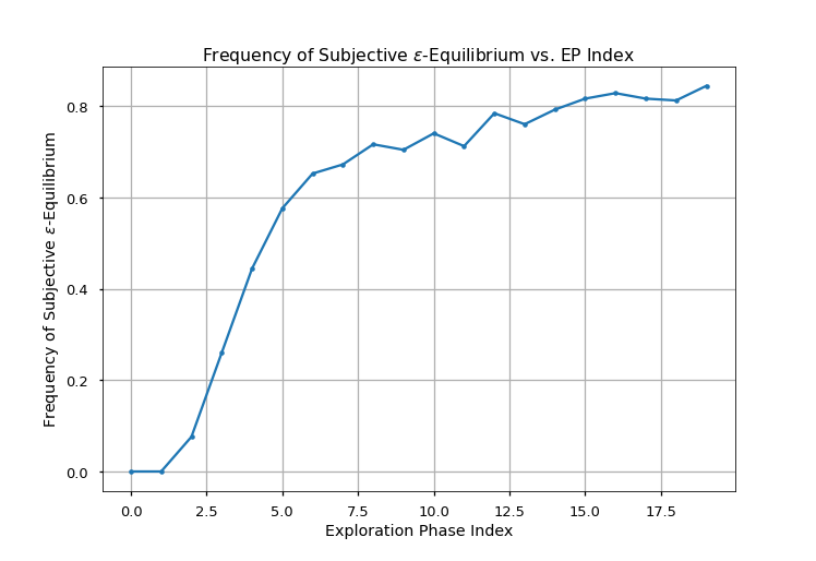
Figure 2: Frequency of subjective $\epsilon$-equilibrium plotted against the exploration phase index, averaged over 250 trials.

Exploration Phase Index $k$	$\frac{1}{250}\sum_{\tau=1}^{250}\textbf{1}\{\bm{\pi}_{k,\tau}\in{\rm Subj}_{\epsilon}(\mathcal{V}^{*},\mathcal{W}^{*})\}$
$k=0$	0.0
$k=5$	$0.576$
$k=10$	$0.74$
$k=15$	$0.816$
$k=19$	$0.844$

Table 1: Frequency of Subjective $\epsilon$-equilibrium. $\bm{\pi}_{k,\tau}$ denotes the policy for EP $k$ during the $\tau^{th}$ trial.

In Figure 3, we plot two curves. The blue curve reports the mean number of agents, out of 20, that are subjectively $\epsilon$-best-responding at a given exploration phase index. This quantity quickly rises to, and remains at, 19.75, reflecting that a great majority of agents are $\epsilon$-satisfied even when the system is not at subjective $\epsilon$-equilibrium. Figure 3 also reports the number of agents using the quantized version of the (presumably) “sensible policy” $\pi_{\rm sensible}\in\mathcal{P}(\mathbb{A}|\mathbb{Y})$ defined as

$$\pi_{\rm sensible}(\cdot|x,\sigma)=\begin{cases}\delta_{\rm go},&\text{ if }x=\text{ good}\\ \delta_{\rm wait},&\text{ if }x=\text{ bad}\\ \delta_{\rm go},&\text{ if }(x,\sigma)=\text{ (medium, low)}\\ \delta_{\rm heal},&\text{ if }(x,\sigma)=\text{ (medium, high) }\end{cases}$$

The orange curve in Figure 3 reports the mean number of agents following the policy ${\rm quant}(\pi_{\rm sensible})$. Interestingly, this curve appears to lag considerably below the blue curve, reflecting that play often settled at an asymmetric joint policy that forms a subjective $\epsilon$-equilibrium.

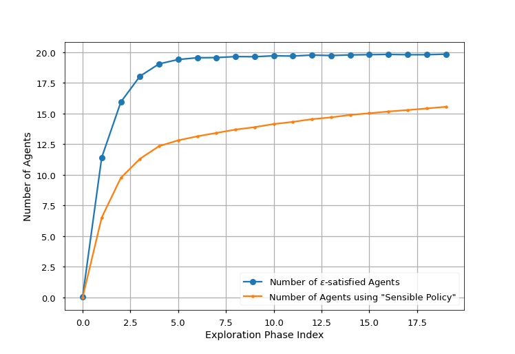
Figure 3: Mean Number of players who are subjective $\epsilon$-best-responding vs. exploration phase index, averaged over 250 trials.

7 Discussion

As previously described, the standard information structure available to players mean-field games is that of mean-field observability (Assumption 2), wherein at time $t\geq 0$, player $i\in\mathcal{N}$ observes its local state $x^{i}_{t}$ and the mean-field state $\mu_{t}=\upmu(\textnormal{{x}}_{t})$, a probability distribution over $\mathbb{X}$. We now consider situations in which compressed observability (Assumption 3) may be the more appropriate model for decentralized information.

To determine the most appropriate observation channel used in the model for a particular application, it is natural to begin by asking how a player’s observations are actually obtained in the application itself. (Here, we emphasize that the actual observation channel encountered need not be the same as the observation channel used in the model of the game.) We envision three (actual) observation channels as being the most plausible:

1. An agent may obtain its own readings on the global state variable through its own local sensors. Such an (actual) observation channel is truly decentralized and would result in a rather limited view of the overall system. Consequently, this may give rise to compressed observability in and of itself, and the actual observation channel may be used as the model’s observation channel.

2. Agents may use local sensors to obtain a partial view of the system, and then supplement this knowledge by communicating with nearby agents. This, too, would give rise to a limited view of the overall system. Here, too, one may naturally take the model’s observation channel to be the same as the actual observation channel, and Assumption 3 may be more appropriate than Assumption 2.

3. Agents may obtain their observations through some type of centralized entity, which monitors the local states of all agents and then computes and broadcasts a (possibly compressed) signal about the mean-field state. For example, in an application where agents are autonomous vehicles, local states are locations in a traffic network, and action selection corresponds to selection of a path to one’s destination, agents may rely on a satellite navigation system to locate themselves in the traffic network and also to identify which road links are congested. In this set-up, if the central entity broadcasts a compressed signal, then the actual observation channel gives rise to compressed observability. Such is the case, for instance, with navigation systems that report road congestion using a three-tiered system of low-, moderate-, and high-congestion road links.

In addition to applications where the actual observation channel results in a limited view of the overall system, compressed observability may also arise in systems with rich (actual) observation channels if players voluntarily choose to discard information in their learning process. When the number of players, $n$, and the number of local states, $|\mathbb{X}|$, are both moderately large, the set of empirical measures ${\rm Emp}_{n}=\{\upmu(\textnormal{{s}}):\textnormal{{s}}\in\textnormal{{X}}\}$ becomes unwieldy for the purposes of (tabular) learning. As such, it is reasonable to expect that naive independent learning agents will employ some form of function approximation, with quantization of ${\rm Emp}_{n}$ offering the simplest form of function approximation. Moreover, a common compression scheme may be shared by all agents in such an application, perhaps as the result of some shared “conventional wisdom” about the system.

8 Conclusion

In this paper, we considered partially observed $n$-player mean-field games from the point of view of decentralized independent learners. Independent learning is characterized by ignoring the presence of other strategic agents in the system, treating one’s environment as if it were a single agent MDP, and naively running single agent learning algorithms to select one’s policy. We studied the convergence of naive single-agent learning iterates in the game setting, proving almost sure convergence under mild conditions on the game. By analogy to near-optimality criteria for MDPs, we used the limiting values of these learning iterates to develop a notion of subjective $\epsilon$-equilibrium for partially observed $n$-player mean-field games. After establishing the existence of objective perfect equilibrium as well as subjective $\epsilon$-equilibrium under mean-field observability, we extended the notion of (objective) $\epsilon$-satisficing paths of Yongacoglu et al. (2023) to subjective value functions. In this framework, we studied the structural properties of $n$-player mean-field games and showed that subjective $\epsilon$-satisficing paths to subjective $\epsilon$-equilibrium exist under various information structures for partially observed $n$-player mean-field games.

Apart from the structural and conceptual contributions described above, we have also presented Algorithm 3, a decentralized independent learner for playing partially observed $n$-player mean-field games, and we have argued that Algorithm 3 drives policies to subjective $\epsilon$-equilibrium under self-play. Unlike the bulk of results on learning in mean-field games, the convergence guarantees of Algorithm 3 do not mandate that players use the same policy at a given time or the same policy update rule to switch policies at the end of an exploration phase. As such, our algorithm is capable of describing learning dynamics for a population of homogenous agents that may arrive at a joint policy consisting of heterogenous policies. The learning dynamics presented here result in system stability, in that policies settle to a particular joint policy, but the emergent behaviour need not be an objective equilibrium. Convergence to non-equilibrium policies may arise in real-world strategic environments, and our notion of subjective equilibrium may present an interpretation for such real-world stability in some instances.

This paper leaves open the question of whether subjective $\epsilon$-equilibrium always exist in mean-field games with compressed or local observability. Determining sufficient conditions for the existence of subjective equilibrium is an interesting topic for future research.

Appendices

Appendix A Fully and Partially Observed Markov Decision Problems

A finite, partially observed Markov decision problem (POMDP) with the discounted cost criterion is given by a list $\mathcal{M}$:

$$\mathcal{M}=\left(\mathcal{X},\mathcal{Y},\mathcal{A},C,P_{\mathcal{M}},\upphi,\upgamma,\upnu_{0}\right).$$ (13)

At time $t\in\mathbb{Z}_{\geq 0}$, the system’s state is denoted $X_{t}$ and takes values in the finite set $\mathcal{X}$, with $X_{0}\sim\upnu_{0}$. An observation $Y_{t}$ taking values in the finite set $\mathcal{Y}$ is generated according to a noisy reading of $X_{t}$ through the observation channel $\upphi\in\mathcal{P}(\mathcal{Y}|\mathcal{X})$, as $Y_{t}\sim\upphi(\cdot|X_{t})$. The agent uses its observable history variable, $\mathcal{h}^{\rm ob}_{t}$, to be defined shortly, to select its action $A_{t}$ from the finite set $\mathcal{A}$. The agent then incurs a stage cost $C_{t}$, given by the cost function $C$ as $C_{t}:=C(X_{t},A_{t})$. The system’s state subsequently evolves according to $X_{t+1}\sim P_{\mathcal{M}}(\cdot|X_{t},A_{t})$, where $P_{\mathcal{M}}\in\mathcal{P}(\mathcal{X}|\mathcal{X}\times\mathcal{A})$. A discount factor $\upgamma\in(0,1)$ is used to discount the sequence of costs incurred by the agent.

We define the system history sets $\{\mathcal{H}_{t}\}_{t\in\mathbb{Z}_{\geq 0}}$ as follows:

$$\mathcal{H}_{t}:=\left(\mathcal{X}\times\mathcal{Y}\times\mathcal{A}\right)^{t}\times\mathcal{X}\times\mathcal{Y},\quad\forall t\geq 0.$$

Elements of $\mathcal{H}_{t}$ are called system histories of length $t$. We define a random quantity $\mathcal{h}_{t}$, taking values in $\mathcal{H}_{t}$ and given by

$$\mathcal{h}_{t}=(X_{0},Y_{0},A_{0},\cdots,X_{t-1},Y_{t-1},A_{t-1},X_{t},Y_{t}),$$

and we use $\mathcal{h}_{t}$ to denote the $t^{\rm th}$ system history variable. To capture the information actually observed by the agent controlling the system, we define observable history sets $\{\mathcal{H}^{\rm ob}_{t}\}_{t\geq 0}$ as

$$\mathcal{H}^{\rm ob}_{t}:=\Delta(\mathcal{X})\times\left(\mathcal{Y}\times\mathcal{A}\times\mathbb{R}\right)^{t}\times\mathcal{Y},\quad\forall t\geq 0.$$

Elements of $\mathcal{H}^{\rm ob}_{t}$ are called observable histories of length $t$, and we let

$$\mathcal{h}^{\rm ob}_{t}=(\upnu_{0},Y_{0},A_{0},C_{0},\cdots,C_{t-1},Y_{t}),$$

denote the $\mathcal{H}^{\rm ob}_{t}$-valued random quantity representing the $t^{\rm th}$ observable history variable.

Definition 26

A sequence $\pi=(\pi_{t})_{t\geq 0}$ such that $\pi_{t}\in\mathcal{P}(\mathcal{A}|\mathcal{H}^{\rm ob}_{t})$ for each $t$ is called a policy for the POMDP $\mathcal{M}$.

We denote the set of all policies for the POMDP $\mathcal{M}$ by $\Pi_{\mathcal{M}}$. Fixing a policy $\pi\in\Pi_{\mathcal{M}}$ and an initial measure $\upnu\in\Delta(\mathcal{X})$ induces a unique probability measure ${\rm Pr}^{\pi}_{\upnu}$ on the trajectories of play, i.e. on sequences $(X_{t},Y_{t},A_{t},C_{t})_{t=0}^{\infty}$. We let $E^{\pi}_{\upnu}$ denote the expectation associated with ${\rm Pr}^{\pi}_{\upnu}$ by define the agent’s objective function as

$$\mathcal{J}_{\mathcal{M}}(\pi,\upnu):=E^{\pi}_{\upnu}\left[\sum_{t\geq 0}\upgamma^{t}C(X_{t},A_{t})\right],\quad\forall\pi\in\Pi_{\mathcal{M}},\upnu\in\Delta(\mathcal{X}).$$

In the special case that $\upnu=\delta_{s}$ for some state $s\in\mathcal{X}$, we simply write $\mathcal{J}_{\mathcal{M}}(\pi,s)$.

Definition 27 (Optimal Policy)

For $\epsilon\geq 0$, a policy $\pi^{*}\in\Pi_{\mathcal{M}}$ is called $\epsilon$-optimal with respect to $\upnu\in\Delta(\mathcal{X})$ if

$$\mathcal{J}_{\mathcal{M}}(\pi^{*},\upnu)\leq\inf_{\pi\in\Pi_{\mathcal{M}}}\mathcal{J}_{\mathcal{M}}(\pi,\upnu)+\epsilon.$$

If $\pi^{*}$ is $\epsilon$-optimal with respect to every $\upnu\in\Delta(\mathcal{X})$, then $\pi^{*}$ is called uniformly $\epsilon$-optimal.

If $\epsilon=0$ in the preceding definition, we simply refer to $\pi^{*}$ as being optimal, either uniformly or with respect to a given initial distribution $\upnu$.

Definition 28 (Stationary Policies)

A policy $\pi\in\Pi_{\mathcal{M}}$ is called (memoryless) stationary (or simply stationary) if, for some $g\in\mathcal{P}(\mathcal{A}|\mathcal{Y})$, the following holds: for any $t\geq 0$ and $\tilde{\mathcal{h}}^{\rm ob}_{t}=(\tilde{\nu},\tilde{Y}_{0},\dots,\tilde{Y}_{t})\in\mathcal{H}^{\rm ob}_{t}$, we have

$$\pi_{t}(\cdot|\tilde{\mathcal{h}}^{\rm ob}_{t})=g(\cdot|\tilde{Y}_{t}).$$

We let $\Pi_{\mathcal{M},S}$ denote the set of stationary policies for the POMDP $\mathcal{M}$.

Definition 29 (Soft Policies)

For $\xi>0$, a policy $\pi\in\Pi_{\mathcal{M}}$ is called $\xi$-soft if, for any $t\geq 0$ and $\tilde{\mathcal{h}}^{\rm ob}_{t}\in\mathcal{H}^{\rm ob}_{t}$, we have $\pi(a|\tilde{\mathcal{h}}^{\rm ob}_{t})\geq\xi$ for all $a\in\mathcal{A}$. A policy $\pi\in\Pi_{\mathcal{M}}$ is called soft if it is $\xi$-soft for some $\xi>0$.

The goal for an agent controlling the POMDP $\mathcal{M}$ is to find an optimal policy.

Remark: We have chosen to present a model in which costs are measurable functions of the state and action. One can also allow for costs to be random variables with expectation given by the cost function $C$. Since our objective involves an expectation, this does not change the ensuing analysis, and we opt for the simpler model.

One can also generalize the POMDP model above (or the MDP model below) to allow the transition/observation probabilities and cost function to additionally depend on time. Such models may be called time inhomogenous. By contrast, the models presented here are time homogenous, as the transition/observation probabilities and cost function do not vary across time. Any reference to a POMDP (or fully observed MDP) in this article shall be understood to refer to a time homogenous POMDP (or MDP).

A.1 Fully Observed Markov Decision Problems

Definition 30 (MDP)

A fully observed Markov decision problem (or simply an MDP) is a POMDP for which $\mathcal{X}=\mathcal{Y}$ and $\upphi(\cdot|s)=\delta_{s}$ for each state $s\in\mathcal{X}$.

It is well-known that if $\mathcal{M}$ is an MDP, then there exists a (uniformly) optimal policy $\pi^{*}\in\Pi_{\mathcal{M},S}$, and furthermore it suffices to check for optimality along Dirac distributions $\{\delta_{s}:s\in\mathcal{X}\}$. Using the existence of an optimal policy $\pi^{*}\in\Pi_{\mathcal{M},S}$, we define the (optimal) Q-function for the MDP $\mathcal{M}$ as follows: $Q^{*}_{\mathcal{M}}:\mathcal{X}\times\mathcal{A}\to\mathbb{R}$ is given by

$$Q^{*}_{\mathcal{M}}(s,a):=E^{\pi^{*}}_{\upnu}\left[\sum_{t=0}^{\infty}\upgamma^{t}C(X_{t},A_{t})\middle|X_{0}=s,A_{0}=a\right],\quad\forall(s,a)\in\mathcal{X}\times\mathcal{A},$$

where $\pi^{*}\in\Pi_{\mathcal{M},S}$ is an optimal policy for $\mathcal{M}$ and $\upnu\in\Delta(\mathcal{X})$ is any initial state distribution. One can show that, for any $s\in\mathcal{X}$, we have $\mathcal{J}_{\mathcal{M}}(\pi^{*},s)=\min_{a\in\mathcal{A}}Q^{*}_{\mathcal{M}}(s,a)$.

Lemma 31

Let $\pi\in\Pi_{\mathcal{M},S}$, $\epsilon\geq 0$. Then, $\pi$ is $\epsilon$-optimal for the MDP $\mathcal{M}$ if and only if

$$\mathcal{J}_{\mathcal{M}}(\pi,s)\leq\min_{a\in\mathcal{A}}Q^{*}_{\mathcal{M}}(s,a)+\epsilon,\quad\forall s\in\mathcal{X}.$$ (14)

Under mild conditions on the MDP $\mathcal{M}$, the action value function $Q^{*}_{\mathcal{M}}$ can be learned iteratively using the Q-learning algorithm Watkins (1989). Similarly, for stationary policies $\pi\in\Pi_{\mathcal{M},S}$, the value function $\mathcal{J}_{\mathcal{M}}(\pi,\cdot)$ can be learned iteratively. That is, the agent can produce sequences of iterates $\{\widehat{J}_{t},\widehat{Q}_{t}\}_{t\geq 0}$, with $\widehat{J}_{t}\in\mathbb{R}^{\mathcal{X}}$ and $\widehat{Q}_{t}\in\mathbb{R}^{\mathcal{X}\times\mathcal{A}}$ for each $t$, such that, almost surely,

$$\widehat{Q}_{t}\to Q^{*}_{\mathcal{M}}\quad\text{and}\quad\widehat{J}_{t}(s)\to\mathcal{J}_{\mathcal{M}}(\pi,s),\quad\forall s\in\mathcal{X}.$$

Thus, an agent controlling the MDP $\mathcal{M}$ using a stationary policy $\pi\in\Pi_{\mathcal{M},S}$ may use an estimated surrogate of the inequality of (14)—involving stochastic estimates of $Q^{*}_{\mathcal{M}}$ and $\mathcal{J}_{\mathcal{M}}(\pi,\cdot)$—as a stopping condition when searching for an $\epsilon$-optimal policy. This idea will feature heavily in the subsequent sections. In particular, we will use an analogous condition for our definition of subjective best-responding. As a preview of forthcoming definitions, we now state a definition that is motivated by analogy to (14).

Definition 32

Let $\widehat{J}\in\mathbb{R}^{\mathcal{X}}$ and $\widehat{Q}\in\mathbb{R}^{\mathcal{X}\times\mathcal{A}}$. The function $\widehat{J}$ is said to be subjectively $\epsilon$-optimal with respect to $\widehat{Q}$ if

$$\widehat{J}(s)\leq\min_{a\in\mathcal{A}}\widehat{Q}(s,a)+\epsilon,\quad\forall s\in\mathcal{X}.$$

The intuition underlying Definition 32 is that $\widehat{J}(s)$ plays the role of $\mathcal{J}_{\mathcal{M}}(\pi,s)$ while $\widehat{Q}(s,a)$ plays the role of $Q^{*}_{\mathcal{M}}(s,a)$ in (14), with $\widehat{J}$ and $\widehat{Q}$ arising from a learning process. In employing such a comparison to test for $\epsilon$-optimality of $\pi$, the agent replaces objective quantities with learned estimates that represent subjective knowledge obtained through system interaction and learning.

Appendix B Implied MDPs and Subjective Functions

In this section, we explicitly characterize the subjective value functions of Theorem 13 in Section 4. These subjective value functions arise as the limit points of an independent learning process, in which each agent used a stationary policy during the learning process and obtained a sequence of stochastic iterates meant to approximate action values and state values of an assumed MDP. However, as described in Lemma 6, each agent does not face a fully observed MDP but rather a POMDP. To understand the limiting values of the learning process in Algorithm 1, we introduce implied MDPs associated with POMDPs. We then use the connection between $n$-player mean-field games and POMDPs to define the subjective functions of Theorem 13 using the language of implied MDPs.

B.1 Implied MDPs and Subjective Functions for Ergodic POMDPs

To begin, let $\mathcal{M}=\left(\mathcal{X},\mathcal{Y},\mathcal{A},C,P_{\mathcal{M}},\upphi,\upgamma,\upnu_{0}\right)$ be a POMDP as described in (13). Recall that $\Pi_{\mathcal{M},S}$ denotes the set of stationary policies for the POMDP $\mathcal{M}$, and is identified with the set $\mathcal{P}(\mathcal{A}|\mathcal{Y})$ of transition kernels on $\mathcal{A}$ given $\mathcal{Y}$. We now define several objects relevant to the analysis of learning algorithms for POMDPs.

Definition 33

For $\lambda\in\Delta(\mathcal{X})$, the backward channel $B^{\lambda}\in\mathcal{P}(\mathcal{X}|\mathcal{Y})$ is a transition kernel on $\mathcal{X}$ given $\mathcal{Y}$ defined by

$$B^{\lambda}(x|y):=\frac{\upphi(y|x)\lambda(x)}{\sum_{s\in\mathcal{X}}\upphi(y|s)\lambda(s)},\quad\forall x\in\mathcal{X},y\in\mathcal{Y}.$$

One may interpret the quantity $B^{\lambda}(x|y)$ as the posterior probability that $x_{0}=x$ given that $x_{0}\sim\lambda$ and the first observation symbol was $y_{0}=y$.

Definition 34

For $\lambda\in\Delta(\mathcal{X})$, the implied transition kernel $\mathcal{T}_{\lambda}\in\mathcal{P}(\mathcal{Y}|\mathcal{Y}\times\mathcal{A})$ is given by

$$\mathcal{T}_{\lambda}(y^{\prime}|y,a):=\sum_{s^{\prime}\in\mathcal{X}}\upphi(y^{\prime}|s^{\prime})\sum_{s\in\mathcal{X}}\mathcal{T}(s^{\prime}|s,a)B^{\lambda}(s|y),\quad\forall y,y^{\prime}\in\mathcal{Y},a\in\mathcal{A}.$$

The quantity $\mathcal{T}_{\lambda}(y^{\prime}|y,a)$ represents the conditional probability that the observation $y_{1}=y^{\prime}$ given $y_{0}=y,u_{0}=u$ and $x_{0}\sim\lambda$.

Definition 35

For $\lambda\in\Delta(\mathcal{X})$, the implied cost function $C_{\lambda}:\mathcal{Y}\times\mathcal{A}\to\mathbb{R}$ is given by

$$C_{\lambda}(y,a):=\sum_{x\in\mathcal{X}}C(x,a)B^{\lambda}(x|y),\quad\forall y\in\mathcal{Y},a\in\mathcal{A}.$$

We will employ the following standing assumption for the remainder of this section.

Assumption 8

For any policy $\pi\in\Pi_{\mathcal{M},S}$, there exists unique $\lambda_{\pi}\in\Delta(\mathcal{X})$ such that

$$\lim_{t\to\infty}{\rm Pr}^{\pi}_{\lambda_{0}}\left(X_{t}\in\cdot\right)=\lambda_{\pi}(\cdot),\quad\forall\lambda_{0}\in\Delta(\mathcal{X}).$$

In words, this assumption says that the law of the hidden state at time $t$, $X_{t}$, converges, as $t\to\infty$, to some invariant ergodic distribution $\lambda_{\pi}\in\Delta(\mathcal{X})$. The invariant distribution will depend on the policy $\pi$, but convergence to this distribution holds for any distribution $\lambda_{0}\in\Delta(\mathcal{X})$ of the initial state $X_{0}$.

Remark: Assumption 8 is made for clarity of presentation, and in fact can be relaxed. For the results below, one can alternatively assume the following.

Assumption 8^⋆ For any policy $\pi\in\Pi_{\mathcal{M},S}$, there exists unique $\lambda_{\pi}\in\Delta(\mathcal{X})$ such that

$$\lim_{T\to\infty}\frac{1}{T}\sum_{t=0}^{T-1}{{\rm Pr}^{\pi}_{\lambda_{0}}}\left(X_{t}\in\cdot\right)=\lambda_{\pi}(\cdot),\quad\forall\lambda_{0}\in\Delta(\mathcal{X}).$$

Under either Assumption 8 or Assumption 8^⋆, each stationary policy is assigned a corresponding backward channel, implied transition kernel, and implied cost function: for each $\pi\in\Pi_{\mathcal{M},S}$, we say that $B^{\lambda_{\pi}}$ is the backward channel associated with $\pi$, $\mathcal{T}_{\lambda_{\pi}}$ is the implied transition kernel associated with $\pi$, and $C_{\lambda_{\pi}}$ is the implied cost unction associated with $\pi$.

For each $\pi\in\Pi_{\mathcal{M},S}$, we define an operator $f_{\pi}:\mathbb{R}^{\mathcal{Y}\times\mathcal{A}}\to\mathbb{R}^{\mathcal{Y}\times\mathcal{A}}$, whose $(y,a)$-component mapping is given by

$$\left[f_{\pi}Q\right](y,a):=C_{\lambda_{\pi}}(y,a)+\gamma\sum_{y^{\prime}\in\mathcal{Y}}\min_{a^{\prime}\in\mathcal{A}}Q(y^{\prime},a^{\prime})\mathcal{T}_{\lambda_{\pi}}(y^{\prime}|y,a),\quad\forall\>Q\in\mathbb{R}^{\mathcal{Y}\times\mathcal{A}}.$$

It is easily verified that $f_{\pi}$ is a $\gamma$-contraction on $\mathbb{R}^{\mathcal{Y}\times\mathcal{A}}$ and therefore admits a unique fixed point, which we denote by $\mathcal{Q}^{*}_{\mathcal{M},\pi}\in\mathbb{R}^{\mathcal{Y}\times\mathcal{A}}$.

Definition 36

The implied Q-function associated with $\pi$ is defined as $\mathcal{Q}^{*}_{\mathcal{M},\pi}$.

Structurally, one can see that the implied Q-function $\mathcal{Q}^{*}_{\mathcal{M},\pi}$ is the optimal Q-function for a suitably defined implied MDP, namely that with state space $\mathcal{Y}$, action space $\mathcal{A}$, stage cost function $C_{\lambda_{\pi}}$, and transition kernel $\mathcal{T}_{\lambda_{\pi}}$.

Remark: To be clear, we do not claim that using the greedy policy with respect to $\mathcal{Q}^{*}_{\mathcal{M},\pi}$ will yield meaningful performance guarantees for the POMDP $\mathcal{M}$.

In addition to the operator $f_{\pi}$, we define an operator $g_{\pi}:\mathbb{R}^{\mathcal{Y}}\to\mathbb{R}^{\mathcal{Y}}$, whose $y$-component mapping is given by

$$\left[g_{\pi}J\right](y):=\sum_{a\in\mathcal{A}}\pi(a|y)\left\{C_{\lambda_{\pi}}(y,a)+\gamma\sum_{y^{\prime}\in\mathcal{Y}}J(y^{\prime})\mathcal{T}_{\lambda_{\pi}}(y^{\prime}|y,a)\right\},\quad\forall J\in\mathbb{R}^{\mathcal{Y}}.$$

As with $f_{\pi}$, one can verify that $g_{\pi}$ is a contraction and admits a unique fixed point, which we denote by $\mathcal{J}^{*}_{\mathcal{M},\pi}\in\mathbb{R}^{\mathcal{Y}}$.

Definition 37

The implied value function associated with $\pi$ is defined as $\mathcal{J}^{*}_{\mathcal{M},\pi}$.

One can interpret the function $\mathcal{J}^{*}_{\mathcal{M},\pi}$ as the state value function of the policy $\pi\in\Pi_{\mathcal{M},S}$ in the same implied MDP as before, with state space $\mathcal{Y}$, action space $\mathcal{A}$, stage cost function $C_{\lambda_{\pi}}$, and transition kernel $\mathcal{T}_{\lambda_{\pi}}$.

B.2 Implied MDPs and Subjective Functions in Partially Observed $n$-Player Mean-Field Games

Let $\textnormal{{G}}=(\mathcal{N},\mathbb{X},\mathbb{Y},\mathbb{A},\{\varphi^{i}\}_{i\in\mathcal{N}},c,\gamma,P_{{\rm loc}},\nu_{0})$ be a partially observed $n$-player mean-field game, with the symbols inheriting their meanings from (1). By Lemma 6, we have that if $\bm{\pi}^{-i}\in\bm{\Pi}^{-i}_{S}$ is a stationary policy for the remaining players, then player $i$ faces a POMDP $\mathcal{M}_{\bm{\pi}^{-i}}$, with partially observed state process $\{\textnormal{{x}}_{t}\}_{t\geq 0}$ and observation process $\{y^{i}_{t}=\varphi^{i}(\textnormal{{x}}_{t})\}_{t\geq 0}$.

Under Assumption 5, if $(\pi^{i},\bm{\pi}^{-i})\in\Pi^{i}_{S}\times\bm{\Pi}^{-i}_{S}$ is stationary, then the ergodicity condition of Assumption 8 holds for the POMDP $\mathcal{M}_{\bm{\pi}^{-i}}$. Thus, for any stationary policy $\pi^{i}\in\Pi^{i}_{S}$, we may define the objects of the preceding section: that is, we may define backward channels, implied transition kernels, implied cost functions, implied Q-functions, and implied value functions associated with $\pi$ in the POMDP $\mathcal{M}_{\bm{\pi}^{-i}}$.

Definition 38

Let G be a partially observed $n$-player mean-field game satisfying Assumption 5. For each player $i\in\mathcal{N}$ and policy $\bm{\pi}^{-i}\in\bm{\Pi}^{-i}_{S}$, let $\mathcal{M}_{\bm{\pi}^{-i}}$ denote the POMDP faced by player $i$.

For any $\bm{\pi}=(\pi^{i},\bm{\pi}^{-i})\in\Pi^{i}_{S}\times\bm{\Pi}^{-i}_{S}$, the subjective value function $V^{*i}_{\bm{\pi}}$ is defined as the implied value function associated with $\pi^{i}$ in the POMDP $\mathcal{M}_{\bm{\pi}^{-i}}$. That is, $V^{*i}_{\bm{\pi}}:={\mathcal{J}^{\star}_{\mathcal{M}_{\bm{\pi}^{-i}},\pi^{i}}}$.

For any $\bm{\pi}=(\pi^{i},\bm{\pi}^{-i})\in\Pi^{i}_{S}\times\bm{\Pi}^{-i}_{S}$, the subjective Q-function $W^{*i}_{\bm{\pi}}$ is defined as the implied Q-function associated with $\pi^{i}$ in the POMDP $\mathcal{M}_{\bm{\pi}^{-i}}$. That is, $W^{*i}_{\bm{\pi}}:={\mathcal{Q}^{\star}_{\mathcal{M}_{\bm{\pi}^{-i}},\pi^{i}}}$.

Appendix C Proof of Lemma 17

For any $i\in\mathcal{N}$, the sets $\bm{\Pi}_{S,{\rm sym}}$ and $\bm{\Pi}^{-i}_{S,{\rm sym}}$ are compact under the topologies induced by the metrics $\textnormal{{d}}_{{\rm sym}}$ and $\textnormal{{d}}^{-i}_{{\rm sym}}$, respectively. By compactness, Lemma 3, and Lemma 10, we see that the functions of Lemmas 3 and 10 are in fact uniformly continuous on $\bm{\Pi}_{S,{\rm sym}}$ and $\bm{\Pi}^{-i}_{S,{\rm sym}}$. It follows that there exists $\xi>0$ such that if two joint policies $\bm{\pi},\bm{\pi}^{\prime}\in\bm{\Pi}_{S,{\rm sym}}$ satisfy $\textnormal{{d}}_{{\rm sym}}(\bm{\pi},\bm{\pi}^{\prime})<\xi$, then

$$\left|J^{i}(\bm{\pi},\textnormal{{s}})-J^{i}(\bm{\pi}^{\prime},\textnormal{{s}})\right|<\frac{\epsilon}{2}\quad\text{and}\quad\left|\min_{a^{i}\in\mathbb{A}}Q^{*i}_{\bm{\pi}^{-i}}(\varphi^{i}(\textnormal{{s}}),a^{i})-\min_{a^{i}\in\mathbb{A}}Q^{*i}_{\bm{\pi}^{\prime-i}}(\varphi^{i}(\textnormal{{s}}),a^{i})\right|<\frac{\epsilon}{2},$$ (15)

for any $\textnormal{{s}}\in\textnormal{{X}}$, where $\varphi^{i}(\textnormal{{s}})=(s^{i},\upmu(\textnormal{{s}}))$ due to Assumption 2. We fix $\bm{\pi}^{*}\in\bm{\Pi}^{0{\rm\text{-}eq}}_{S}\cap\bm{\Pi}_{{\rm sym}}$ to be a symmetric perfect equilibrium policy, which exists by Theorem 12. (That a symmetric perfect equilibrium exists can be seen from the proof of Theorem 12.) Let $\bm{\pi}_{\rm soft}\in\bm{\Pi}_{S,{\rm sym}}$ be a soft, symmetric joint policy satisfying $\textnormal{{d}}_{{\rm sym}}(\bm{\pi}^{*},\bm{\pi}_{\rm soft})<\xi$.

By part 3 of Theorem 13, since $\bm{\pi}_{\rm soft}$ is soft, we have that

$$W^{*i}_{\bm{\pi}_{\rm soft}}=Q^{*i}_{\bm{\pi}^{-i}_{\rm soft}}\quad\text{and}\quad V^{*i}_{\bm{\pi}_{\rm soft}}(\varphi^{i}(\textnormal{{s}}))=J^{i}(\bm{\pi}_{\rm soft},\textnormal{{s}}),\quad\forall i\in\mathcal{N},\textnormal{{s}}\in\textnormal{{X}}.$$

Combining this with (15), it follows that, for any $\textnormal{{s}}\in\textnormal{{X}}$ and $i\in\mathcal{N}$, we have $V^{*i}_{\bm{\pi}_{\rm soft}}(\varphi^{i}(\textnormal{{s}}))\leq\min_{a^{i}\in\mathbb{A}}W^{*i}_{\bm{\pi}_{\rm soft}}(\varphi^{i}(\textnormal{{s}}),a^{i})+\epsilon$, which shows that $\bm{\pi}_{\rm soft}\in{\rm Subj}_{\epsilon}(\mathcal{V}^{*},\mathcal{W}^{*})$. $\square$

Appendix D Proof of Lemma 24

To prove Lemma 24, we first need an auxiliary result.

Lemma 39

Let G be a partially observed $n$-player mean-field game for which Assumptions 2 and 5 hold, and let $\epsilon\geq 0$. Let $\bm{\pi}\in\bm{\Pi}_{S}$ be soft. For $i,j\in\mathcal{N}$, suppose $\pi^{i}$ and $\pi^{j}$ are symmetric. Then, we have

$$\pi^{i}\in{\rm Subj\text{-}BR}^{i}_{\epsilon}(\bm{\pi}^{-i},\mathcal{V}^{*},\mathcal{W}^{*})\iff\pi^{j}\in{\rm Subj\text{-}BR}^{j}_{\epsilon}(\bm{\pi}^{-j},\mathcal{V}^{*},\mathcal{W}^{*}).$$

Proof  To prove this result, we argue that the subjective functions of players $i$ and $j$ satisfy $V^{*i}_{\bm{\pi}}=V^{*j}_{\bm{\pi}}$ and $W^{*i}_{\bm{\pi}}=W^{*j}_{\bm{\pi}}$ whenever $\pi^{i}$ and $\pi^{j}$ are symmetric and soft. In Section 4, we observed that, under Assumptions 2 and 5, the learned values $V^{*i}_{\bm{\pi}}$ and $W^{*i}_{\bm{\pi}}$ were in fact the state value and action value functions, respectively, for an MDP with state space $\{\varphi^{i}(\textnormal{{s}}):\textnormal{{s}}\in\textnormal{{X}}\}\subseteq\mathbb{Y}$. An analogous remark holds for $V^{*j}_{\bm{\pi}}$ and $W^{*j}_{\bm{\pi}}$ and player $j$. The MDP in question was called an approximate belief MDP by Kara and Yüksel (2022), and can be characterized in terms of the implied MDP construction of Appendix B.

We will argue that the approximate belief MDP on $\{\varphi^{i}(\textnormal{{s}}):\textnormal{{s}}\in\textnormal{{X}}\}$ faced by player $i$ is equivalent to the approximate belief MDP on $\{\varphi^{j}(\textnormal{{s}}):\textnormal{{s}}\in\textnormal{{X}}\}$ faced by player $j$. Then, since player $i$ and $j$’s policies are symmetric, they correspond to the same stationary policy for this approximate belief MDP, and are therefore both either $\epsilon$-optimal for that MDP or not; the result will follow.

To see that the approximate belief MDP facing player $i$ is equivalent to that facing player $j$, we observe that the construction of Kara and Yüksel (2022) depends only on the stage cost function, the observation channel, and the unique invariant distribution on the underlying state space. The stage cost and observation channel are symmetric and shared by players $i$ and $j$, so it suffices to show that the unique invariant distribution on X, say $\nu_{\bm{\pi}}$, is symmetric in the following sense:

$$\nu_{\bm{\pi}}({\rm swap}_{ij}(\textnormal{{s}}))=\nu_{\bm{\pi}}(\textnormal{{s}}),\quad\forall\textnormal{{s}}\in\textnormal{{X}},$$ (16)

where, for any $\textnormal{{s}}\in\textnormal{{X}}$, ${\rm swap}_{ij}(\textnormal{{s}})\in\textnormal{{X}}$ is the global state satisfying (1) ${\rm swap}_{ij}(\textnormal{{s}})^{p}=s^{p}$ for each $p\in\mathcal{N}\setminus\{i,j\}$, and (2) we have ${\rm swap}_{ij}(\textnormal{{s}})^{j}=s^{i}$ and ${\rm swap}_{ij}(\textnormal{{s}})^{i}=s^{j}$.

To see that (16) holds, note that by Assumption 5, $\{\textnormal{{x}}_{t}\}_{t\geq 0}$ is an irreducible, aperiodic Markov chain on X under the soft policy $\bm{\pi}$. Thus, we have for any $\tilde{\nu}\in\Delta(\textnormal{{X}})$.

$${\rm Pr}^{\bm{\pi}}_{\tilde{\nu}}(\textnormal{{x}}_{t}\in\cdot)\to\nu_{\bm{\pi}}(\cdot),$$

as $t\to\infty$, where $\nu_{\bm{\pi}}$ is the (unique) invariant measure on X induced by $\bm{\pi}$. In particular, putting the initial measure $\tilde{\nu}=\text{Unif}(\textnormal{{X}})$, we have that for each $t\geq 0$ and each $\textnormal{{s}}\in\textnormal{{X}}$,

$${\rm Pr}^{\bm{\pi}}_{\tilde{\nu}}(\textnormal{{x}}_{t}=\textnormal{{s}})={\rm Pr}^{\bm{\pi}}_{\tilde{\nu}}(\textnormal{{x}}_{t}={\rm swap}_{ij}(\textnormal{{s}})).$$

It follows that

$$\nu_{\bm{\pi}}(\textnormal{{s}}):=\lim_{t\to\infty}{\rm Pr}^{\bm{\pi}}_{\tilde{\nu}}(\textnormal{{x}}_{t}=\textnormal{{s}})=\lim_{t\to\infty}{\rm Pr}^{\bm{\pi}}_{\tilde{\nu}}(\textnormal{{x}}_{t}={\rm swap}_{ij}(\textnormal{{s}}))=:\nu_{\bm{\pi}}({\rm swap}_{ij}(\textnormal{{s}})).$$

From this, it follows that the approximate belief MDP on $\mathbb{Y}$ faced by player $i$ is the same as the approximate belief MDP on $\mathbb{Y}$ faced by player $j$.  

Proof of Lemma 24

We have that $\{\bm{\pi}_{k}\}_{k\geq 0}$ is a time homogenous Markov chain on $\widehat{\bm{\Pi}}$. For any subjective $\epsilon$-equilibrium $\bm{\pi}^{*}\in\widehat{\bm{\Pi}}\cap{\rm Subj}_{\epsilon}(\mathcal{V}^{*},\mathcal{W}^{*})$, we have that the singleton $\{\bm{\pi}^{*}\}$ is an absorbing set for this Markov chain. By part 2 of Lemma 23, the game G has the $(\mathcal{V}^{*},\mathcal{W}^{*})$-subjective $\epsilon$-satisficing paths property in $\widehat{\bm{\Pi}}$. For any $\bm{\pi}\in\widehat{\bm{\Pi}}$, let $L_{\bm{\pi}}<\infty$ denote the length of a shortest $(\mathcal{V}^{*},\mathcal{W}^{*})$-subjective $\epsilon$-satisficing path within $\widehat{\bm{\Pi}}$ that starts at $\bm{\pi}$ and terminates at a policy in $\widehat{\bm{\Pi}}\cap{\rm Subj}_{\epsilon}(\mathcal{V}^{*},\mathcal{W}^{*})$. Call such a policy $\bm{\pi}^{*}$ and note it depends on $\bm{\pi}$. We also define $p_{\bm{\pi}}>0$ as the probability the Markov chain follows this path when starting at $\bm{\pi}$, i.e.

$$p_{\bm{\pi}}:={\rm Pr}(\bm{\pi}_{L_{\bm{\pi}}}=\bm{\pi}^{*}|\bm{\pi}_{0}=\bm{\pi})>0,\quad\forall\bm{\pi}\in\widehat{\bm{\Pi}}.$$

Define $L:=\max\{L_{\bm{\pi}}:\bm{\pi}\in\widehat{\bm{\Pi}}\}$ and $\hat{p}:=\min\{p_{\bm{\pi}}:\bm{\pi}\in\widehat{\bm{\Pi}}\}>0$. For any $m\geq 0$, we have

$${\rm Pr}\left(\bigcap_{j=1}^{m}\{\bm{\pi}_{jL}\notin\widehat{\bm{\Pi}}\cap{\rm Subj}_{\epsilon}(\mathcal{V}^{*},\mathcal{W}^{*})\}\right)\leq(1-\hat{p})^{m}.$$

Taking $m\to\infty$ gives the result.

Appendix E Approximation Results on the Sequences of Learning Iterates

Remark: The contents of this and the next section closely resembles that of (Yongacoglu et al., 2023, Appendix A). The proof technique used here parallels the proof technique of (Yongacoglu et al., 2023, Theorem 5.1).

In the coming sections, we prove that Algorithm 3 leads to the convergence of joint policies as described in Theorems 25, 57, and 58. Since the evolution of the policy process $\{\bm{\pi}_{k}\}_{k\geq 0}$ depends on the evolution of the learning iterates $\{\widehat{J}^{i}_{t},\widehat{Q}^{i}_{t}\}_{t\geq 0,i\in\mathcal{N}}$, we begin by studying the convergence behaviour of these iterates. We argue that if parameters are suitably selected, then these learning iterates sampled at the end of each exploration phase will closely approximate the subjective functions for that exploration phase, and consequently the policy process of Algorithm 3 approximates the policy process of the Markov chain resulting from Algorithm 2.

We note that when each agent $i\in\mathcal{N}$ uses Algorithm 3, it is actually following a particular randomized, non-stationary policy. When all agents use Algorithm 3, we use ${\rm Pr}$ (with no policy index in the superscript and optional initial distribution in the subscript, e.g. ${\rm Pr}_{\nu}$ for some $\nu\in\Delta(\textnormal{{X}})$) to denote the resulting probability measure on trajectories of states and actions. For all other policies $\tilde{\bm{\pi}}\in\bm{\Pi}$, we continue to use ${\rm Pr}^{\tilde{\bm{\pi}}}_{\nu}$, as before.

The policy process $\{\bm{\pi}_{k}\}_{k\geq 0}$ depends on the sequences $\{\widehat{J}^{i}_{t},\widehat{Q}^{i}_{t}\}_{t\geq 0,i\in\mathcal{N}}$ only through these sequences sampled at the end of exploration phases; that is, the iterate sequences are relevant to the updating of policies only along the subsequence of times $\{t_{k}\}_{k\geq 0}$. Recall that we used $\{\bar{Q}^{i}_{t}\}_{t\geq 0}$ and $\{\bar{J}^{i}_{t}\}_{t\geq 0}$ to denote the naively learned stochastic iterates obtained when player $i\in\mathcal{N}$ employed Algorithm 1 and all players followed a soft stationary policy. We now analyze the sequences $\{\widehat{Q}^{i}_{t}\}_{t\geq 0}$ and $\{\widehat{J}^{i}_{t}\}_{t\geq 0}$ by comparison to the sequences $\{\bar{Q}^{i}_{t}\}_{t\geq 0}$ and $\{\bar{J}^{i}_{t}\}_{t\geq 0}$.

The sequences $\{\widehat{Q}^{i}_{t}\}_{t\geq 0}$ and $\{\bar{Q}^{i}_{t}\}_{t\geq 0}$ are related through the Q-factor update. There are, however, two major differences. First, Algorithm 3 instructs player $i$ to reset its counters at the end of the $k^{th}$ exploration phase (i.e. after the update at time $t_{k+1}$, before the update at time $t_{k+1}+1$), meaning the step sizes differ for the two iterate sequences $\{\bar{Q}^{i}_{t}\}_{t\geq 0}$ and $\{\widehat{Q}^{i}_{t}\}_{t\geq 0}$ even when the state-action-cost trajectories observed by player $i$ are identical. Second, Algorithm 3 instructs player $i$ to reset its Q-factors at the end of the $k^{th}$ exploration phase, while Algorithm 1 does not involve any resetting.

Consequently, one sees that the process $\{\widehat{Q}^{i}_{t}\}_{t\geq 0}$ depends on the initial condition $\widehat{Q}^{i}_{0}=0\in\mathbb{R}^{\mathbb{Y}\times\mathbb{A}}$, the state-action trajectory, and the resetting times $\{t_{k}\}_{k\geq 0}$. In contrast, the process $\{\bar{Q}^{i}_{t}\}_{t\geq 0}$ depends only on the initial value $\bar{Q}^{i}_{0}=0\in\mathbb{R}^{\mathbb{Y}\times\mathbb{A}}$ and the state-action trajectory. Analogous remarks hold relating $\{\widehat{J}^{i}_{t}\}_{t\geq 0}$ and $\{\bar{J}^{i}_{t}\}_{t\geq 0}$.

Recall that the $k^{th}$ exploration phase begins with the stage game at time $t_{k}$ and ends before the stage game at time $t_{k+1}=t_{k}+T_{k}$. During the $k^{th}$ exploration phase, the sequences $\{\widehat{Q}^{i}_{t}\}_{t=t_{k}}^{t_{k}+T_{k}}$ and $\{\widehat{J}^{i}_{t}\}_{t=t_{k}}^{t_{k}+T_{k}}$ depend only on the the state-action trajectory $\textnormal{{x}}_{t_{k}},\textnormal{{a}}_{t_{k}},\cdots,\textnormal{{a}}_{t_{k}+T_{k}-1},\textnormal{{x}}_{t_{k}+T_{k}}$. This leads to the following useful observation:

$${\rm Pr}\left(\{\textnormal{{x}}_{t_{k}+T_{k}}=\textnormal{{s}}_{T_{k}}\}\bigcap_{j=0}^{T_{k}-1}\{\textnormal{{x}}_{t_{k}+j}=\textnormal{{s}}_{j},\textnormal{{a}}_{t_{k}+j}=\tilde{\textnormal{{a}}}_{j}\}\middle|\textnormal{{x}}_{t_{k}}=\textnormal{{s}},\bm{\pi}_{k}=\bm{\pi}\right)$$

$$= {\rm Pr}^{\bm{\pi}}_{\textnormal{{s}}}\left(\{\textnormal{{x}}_{T_{k}}=\textnormal{{s}}_{T_{k}}\}\bigcap_{j=0}^{T_{k}-1}\{\textnormal{{x}}_{j}=\textnormal{{s}}_{j},\textnormal{{a}}_{j}=\tilde{\textnormal{{a}}}_{j}\}\right),$$

holds for any $(\textnormal{{s}}_{0},\textnormal{{s}}_{1},\cdots,\textnormal{{s}}_{T_{k}})\in\textnormal{{X}}^{T_{k}+1}$ and $(\tilde{\textnormal{{a}}}_{0},\cdots,\tilde{\textnormal{{a}}}_{T_{k}-1})\in\textnormal{{A}}^{T_{k}}$, where $\textnormal{{A}}=\times_{i\in\mathcal{N}}\mathbb{A}$.

In words, once players following Algorithm 3 select a policy $\bm{\pi}$ for the $k^{th}$ exploration phase, then the conditional probabilities of the trajectories restricted to time indices in that exploration phase can be described by ${\rm Pr}^{\bm{\pi}}$, with the indices of the events suitably shifted to start at time 0. This leads to a series of useful lemmas, which we include below for completeness.

Lemma 40

For any $i\in\mathcal{N},\bm{\pi}\in\widehat{\bm{\Pi}},k\geq 0$ and global state $\textnormal{{s}}\in\textnormal{{X}}$, we have

$${\rm Pr}\left(\widehat{Q}^{i}_{t_{k+1}}\in\cdot\middle|\bm{\pi}_{k}=\bm{\pi},\textnormal{{x}}_{t_{k}}=\textnormal{{s}}\right)={\rm Pr}^{\bm{\pi}}_{\textnormal{{s}}}\left(\bar{Q}^{i}_{T_{k}}\in\cdot\right)$$

and

$${\rm Pr}\left(\widehat{J}^{i}_{t_{k+1}}\in\cdot\middle|\bm{\pi}_{k}=\bm{\pi},\textnormal{{x}}_{t_{k}}=\textnormal{{s}}\right)={\rm Pr}^{\bm{\pi}}_{\textnormal{{s}}}\left(\bar{J}^{i}_{T_{k}}\in\cdot\right).$$

Combining Lemma 40 with Theorem 13, we get the following result.

Lemma 41

For any joint policy $\bm{\pi}\in\widehat{\bm{\Pi}}$, global state $\textnormal{{s}}\in\textnormal{{X}}$, and player $i\in\mathcal{N}$, we have

1. ${\rm Pr}^{\bm{\pi}}_{\textnormal{{s}}}\left(\lim_{t\to\infty}\bar{Q}^{i}_{t}=W^{*i}_{\bm{\pi}}\right)=1$.

2. ${\rm Pr}^{\bm{\pi}}_{\textnormal{{s}}}\left(\lim_{t\to\infty}\bar{J}^{i}_{t}=V^{*i}_{\bm{\pi}}\right)=1$.

3. For any $\xi>0$, there exists $T=T(i,\bm{\pi},\xi)\in\mathbb{N}$ such that

   $${\rm Pr}^{\bm{\pi}}_{\textnormal{{s}}}\left(\sup_{t\geq T}\left\|\bar{Q}^{i}_{t}-W^{*}_{\bm{\pi}}\right\|_{\infty}<\xi\right)\geq 1-\xi,\text{ and }{\rm Pr}^{\bm{\pi}}_{\textnormal{{s}}}\left(\sup_{t\geq T}\left\|\bar{J}^{i}_{t}-V^{*}_{\bm{\pi}}\right\|_{\infty}<\xi\right)\geq 1-\xi$$

Finally, we combine Lemmas 40 and 41 to obtain the following useful result on conditional probabilities.

Lemma 42

Let $k,\ell\in\mathbb{Z}_{\geq 0}$ and suppose $k\leq\ell$. Let $\mathcal{F}_{k}$ denote the $\sigma$-algebra generated by the random variables $\bm{\pi}_{k}$ and $\textnormal{{x}}_{t_{k}}$. For any $\xi>0$, there exists $T=T(\xi)\in\mathbb{N}$ such that if $T_{\ell}\geq T$, then ${\rm Pr}$-almost surely, we have

$${\rm Pr}\left(\bigcap_{i\in\mathcal{N}}\left\{\left\|\widehat{Q}^{i}_{t_{\ell+1}}-W^{*i}_{\bm{\pi}_{\ell}}\right\|_{\infty}<\xi\right\}\cap\left\{\left\|\widehat{J}^{i}_{t_{\ell+1}}-V^{*i}_{\bm{\pi}_{\ell}}\right\|_{\infty}<\xi\right\}\middle|\mathcal{F}_{k}\right)\geq 1-\xi.$$

Appendix F Proof of Theorem 25

We begin by introducing the quantity $\bar{d}_{{\rm MF}}$, which will serve as the upper bound for the tolerance parameters $d^{i},i\in\mathcal{N}$. The quantity $\bar{d}_{{\rm MF}}$, depends on both $\epsilon>0$ and the subset of policies $\widehat{\bm{\Pi}}\subset\bm{\Pi}_{S}$ as follows: $\bar{d}_{{\rm MF}}:=\min\mathcal{O}_{{\rm MF}}$, where $\mathcal{O}_{{\rm MF}}:=S_{{\rm MF}}\setminus\{0\}$, and $S_{{\rm MF}}$ is given by

$$S_{{\rm MF}}:=\left\{\left|\epsilon-\left(V^{*i}_{\bm{\pi}}(y)-\min_{a^{i}\in\mathbb{A}}W^{*i}_{\bm{\pi}}(y,a^{i})\right)\right|:i\in\mathcal{N},\bm{\pi}\in\widehat{\bm{\Pi}},y\in\mathbb{Y}\right\}.$$

That is, $S_{{\rm MF}}$ is the collection of (subjective) $\epsilon$-optimality gaps of the various joint policies in $\widehat{\bm{\Pi}}$, and $\bar{d}_{{\rm MF}}$ is the minimum non-zero separation between $\epsilon$ and the (subjective) suboptimality gap of some player $i$’s performance.

In Assumption 7, we assumed that each player’s $d^{i}$ parameter, which represents tolerance for suboptimality in their policy evaluation step and is included to account for noise in the learning iterates, is positive and small: $d^{i}\in(0,\bar{d}_{{\rm MF}})$ for each $i\in\mathcal{N}$.

We define $\Xi:=\frac{1}{2}\min_{i\in\mathcal{N}}\{d^{i},\bar{d}_{{\rm MF}}-d^{i}\}$. The quantity $\Xi$ will serve as a desirable upper bound on learning error: if players jointly follow a joint policy $\bm{\pi}\in\widehat{\bm{\Pi}}$ and engage in Q-learning and value function estimation, then convergence to within $\Xi$ of the limiting values ensures that each player correctly assesses whether it is $(\mathcal{V}^{*},\mathcal{W}^{*})$-subjectively $\epsilon$-best-responding by using the comparison of Line 17 of Algorithm 3. We formalize this below.

For $k\geq 0$, we define ${\rm Event}(\Xi,k)$ as

$${\rm Event}(\Xi,k):=\left\{\max\left\{\|\widehat{J}^{i}_{t_{k+1}}-V^{*i}_{\bm{\pi}_{k}}\|_{\infty},\|\widehat{Q}^{i}_{t_{k+1}}-W^{*i}_{\bm{\pi}_{k}}\|_{\infty}:i\in\mathcal{N}\right\}<\Xi\right\}.$$

Given ${\rm Event}(\Xi,k)$, we have that for any player $i\in\mathcal{N}$,

$$\pi^{i}_{k}\in{\rm Subj\text{-}BR}^{i}_{\epsilon}(\bm{\pi}^{-i}_{k},\mathcal{V}^{*},\mathcal{W}^{*})\iff\widehat{J}^{i}_{t_{k+1}}(\varphi^{i}(\textnormal{{x}}))\leq\min_{a^{i}\in\mathbb{A}}\widehat{Q}^{i}_{t_{k+1}}(\varphi^{i}(\textnormal{{x}}),a^{i})+\epsilon+d^{i}\quad\forall\textnormal{{x}}\in\textnormal{{X}}.$$

For convenience, we also define the following intersection of events. For any $k,\ell\in\mathbb{Z}_{\geq 0}$, let

$$E_{k:k+\ell}:=\cap_{j=0}^{\ell}{\rm Event}(\Xi,k+j).$$

That is, $E_{k:k+\ell}$ is the event where all agents obtain $\Xi$-accurate learning estimates in each of the exploration phases $k,k+1,\cdots,k+\ell$. For $k\in\mathbb{Z}_{\geq 0}$, we let $G_{k}$ denote the event that the policy $\bm{\pi}_{k}$ is an $\epsilon$-equilibrium: $G_{k}:=\{\bm{\pi}_{k}\in\bm{\Pi}\cap{\rm Subj}_{\epsilon}(\mathcal{V}^{*},\mathcal{W}^{*})\}$.

From the preceding discussion on $\bar{d}_{{\rm MF}},\{d^{i}\}_{i\in\mathcal{N}}$ and the choice of $\Xi$, we have that for any $\ell\geq 0$,

$${\rm Pr}\left(G_{k+\ell}\middle|G_{k}\cap E_{k:k+\ell}\right)=1.$$ (17)

Recall the quantity $L:=\max\{L_{\bm{\pi}_{0}}:\bm{\pi}_{0}\in\widehat{\bm{\Pi}}\}$, where for each $\bm{\pi}_{0}\in\widehat{\bm{\Pi}}$, the number $L_{\bm{\pi}_{0}}<\infty$ is defined as the shortest $(\mathcal{V}^{*},\mathcal{W}^{*})$-subjective $\epsilon$-satisficing path within $\widehat{\bm{\Pi}}$ starting at $\bm{\pi}_{0}$ and ending in $\widehat{\bm{\Pi}}\cap{\rm Subj}_{\epsilon}(\mathcal{V}^{*},\mathcal{W}^{*})$. From our assumptions on $\widehat{\bm{\Pi}}$, such a path exists for every $\bm{\pi}_{0}\in\widehat{\bm{\Pi}}$. If $L_{\bm{\pi}_{0}}<L$ for a particular initial policy $\bm{\pi}_{0}$, we may extend this path to have length $L$ by repeating the final term. Thus, for every $\bm{\pi}\in\widehat{\bm{\Pi}}$, we obtain the inequality

$${\rm Pr}\left(G_{k+L}\middle|\{\bm{\pi}_{k}=\bm{\pi}\}\cap E_{k:k+L}\right)\geq p_{\min}>0,$$ (18)

where $p_{\min}:=\prod_{i\in\mathcal{N}}\left(\frac{e^{i}}{|\widehat{\Pi}^{i}|}\right)^{L}>0$. The bound $p_{\min}$ is obtained through the following loose lower bounding argument: beginning at $\bm{\pi}_{k}=\bm{\pi}$, the joint policy process $\bm{\pi}_{k},\dots,\bm{\pi}_{k+L}$ follows the $(\mathcal{V}^{*},\mathcal{W}^{*})$-subjective $\epsilon$-satificing path of length $L$ described above with probability no less than the event that—at each step—the “correct” unsatisfied player updates to the “correct” policy uniformly at random, which occurs with probability no less than the probability given by the ratio in the product.

Fix $u^{*}\in(0,1)$ such that

$$\frac{u^{*}p_{\min}}{1-u^{*}+u^{*}p_{\min}}>1-\frac{\xi}{2}.$$

Combining Lemma 42 with a union bound, we have that there exists $\tilde{T}\in\mathbb{N}$ such that if $T_{l}>\tilde{T}$ for all $l\geq 0$, then ${\rm Pr}\left(E_{k:k+L}|\bm{\pi}_{k}=\bm{\pi}\right)\geq u^{*}$ for all $k\geq 0$ and any $\bm{\pi}\in\widehat{\bm{\Pi}}$. Thus, we have ${\rm Pr}\left(E_{k:k+L}\middle|G_{k}\right)\geq u^{*}$ and ${\rm Pr}\left(E_{k:k+L}\middle|G^{c}_{k}\right)\geq u^{*}$ for each $k\geq 0$.

We now lower bound ${\rm Pr}(G_{k+L})$ by conditioning on $G_{k}$ and $G_{k}^{c}$ as follows.

$${\rm Pr}\left(G_{k+L}\right)={\rm Pr}(G_{k+L}|G_{k}){\rm Pr}(G_{k})+{\rm Pr}(G_{k+L}|G_{k}^{c})(1-{\rm Pr}(G_{k})).$$

We then lower bound each of the terms above by conditioning on $E_{k:k+L}$ and invoking inequalities (17) and (18):

$${\rm Pr}(G_{k+L})\geq 1\cdot{\rm Pr}(E_{k:k+L}|G_{k})\cdot{\rm Pr}(G_{k})+p_{\min}{\rm Pr}(E_{k:k+L}|G_{k}^{c})(1-{\rm Pr}(G_{k})).$$

Assume now that $T_{l}>\tilde{T}$ for all $l\geq 0$. We have

$${\rm Pr}(G_{k+L})\geq u^{*}{\rm Pr}(G_{k})+u^{*}p_{\min}(1-{\rm Pr}(G_{k})),\quad\forall k\geq 0.$$

For each $k\in\{0,1,\dots,L-1\}$, define $y^{(k)}_{0}:={\rm Pr}(G_{k})$, and for $m\geq 0$ define $y^{(k)}_{m+1}:=u^{*}y^{(k)}_{m}+u^{*}p_{\min}\left(1-y^{(k)}_{m}\right).$ By induction, one can show that

$${\rm Pr}(G_{k+mL})\geq y^{(k)}_{m},\quad\forall m\geq 0.$$ (19)

Observe that $y^{(k)}_{m+1}$ can be written as

$$y^{(k)}_{m+1}=\left(u^{*}-u^{*}p_{\min}\right)^{m+1}y^{(k)}_{0}+u^{*}p_{\min}\sum_{j=0}^{m}\left(u^{*}-u^{*}p_{\min}\right)^{j}.$$

Since $0<u^{*}-u^{*}p_{\min}<1$, we have that $\lim_{m\to\infty}y^{(k)}_{m}=\frac{u^{*}p_{\min}}{1-u^{*}+u^{*}p_{\min}}>1-\frac{\xi}{2}$. Then, by (19), we have that ${\rm Pr}(G_{k+mL})\geq 1-\xi/2$ holds for all sufficiently large $m$, which completes the proof.

Appendix G An Approximation Result Relating to Mean-Field Equilibrium

In this section, we present results relating various solution concepts in mean-field games. The aim of this section is to suggest how one may use approximation results to establish the existence of subjective $\epsilon$-equilibrium in partially observed $n$-player mean-field games with local observability. We begin by introducing the concept of stationary mean-field equilibrium (SMFE) and giving sufficient conditions for the existence of SMFE. We then argue that, under some additional conditions on the transition probabilities, a SMFE can be used to obtain an (objective) $\epsilon$-equilibrium for a particular partially observed $n$-player mean-field game with sufficiently large $n$. We conclude this section with high-level discussion on how these results can be used to establish existence of subjective $\epsilon$-equilibrium.

G.1 Mean-Field System

To facilitate passing from a model with finitely many players to a model with infinitely many players, we now introduce the terminology of mean-field systems, upon which the games will be defined or re-defined. The mean-field system underlying the mean-field game is a partial list of problem data, $G$, given by

$$G=(\mathbb{X},\mathbb{A},c,P_{{\rm loc}},\gamma).$$

The symbols in $G$ retain their earlier meanings: $\mathbb{X}$ is a finite set of states, $\mathbb{A}$ is a finite set of actions, $c:\mathbb{X}\times\Delta(\mathbb{X})\times\mathbb{A}\to\mathbb{R}$ is a cost function, $P_{{\rm loc}}\in\mathcal{P}(\mathbb{X}|\mathbb{X}\times\Delta(\mathbb{X})\times\mathbb{A})$ is a local state transition kernel, and $\gamma\in(0,1)$ is a discount factor.

G.2 Mean-Field MDPs

We now introduce a family of single-agent MDPs, denoted M, whose elements are indexed by mean-field terms in $\Delta(\mathbb{X})$. For each $\nu\in\Delta(\mathbb{X})$, we let

$$\mathcal{M}_{\nu}=(\mathbb{X},\mathbb{A},c_{\nu},P_{\nu},\gamma)$$

be the MDP with state space $\mathbb{X}$, action set $\mathbb{A}$, discount factor $\gamma$, and where the stage cost function $c_{\nu}$ and transition kernel $P_{\nu}$ are given by

$$P_{\nu}(\cdot|x,a):=P_{{\rm loc}}(\cdot|x,\nu,a),\quad c_{\nu}(x,a):=c(x,\nu,a),\quad\forall(x,a)\in\mathbb{X}\times\mathbb{A}.$$

To be clear, $\nu\in\Delta(\mathbb{X})$ need not be the initial distribution for the MDP $\mathcal{M}_{\nu}$: it is used merely to define the cost function and state transition probabilities by fixing the mean-field term at $\nu$. In this section, any MDP of this form is called a mean-field MDP.

We let $\textnormal{{M}}:=\{\mathcal{M}_{\nu}:\nu\in\Delta(\mathbb{X})\}$. For each MDP $\mathcal{M}_{\nu}\in\textnormal{{M}}$, the history sets are defined as $H_{0}:=\mathbb{X}$ and $H_{t+1}:=H_{t}\times\mathbb{A}\times\mathbb{X}$ for each $t\geq 0$. An admissible policy is defined as a sequence of transition kernels $\pi=(\pi_{t})_{t\geq 0}$ such that $\pi_{t}\in\mathcal{P}(\mathbb{A}|H_{t})$ for each $t\geq 0$. The set of all policies for any MDP $\mathcal{M}_{\nu}\in\textnormal{{M}}$ is denoted by $\Pi_{\textnormal{{M}}}$, and we note that this set of admissible policies is common to every MDP in M. As usual, $\Pi_{\textnormal{{M}},S}$ denotes the set of stationary policies. Here, we identify stationary policies with transition kernels in $\mathcal{P}(\mathbb{A}|\mathbb{X})$.

In accordance with the notation of Section A.1, the objective function for the MDP $\mathcal{M}_{\nu}$ controlled by policy $\pi\in\Pi_{\textnormal{{M}}}$ is denoted

$$\mathcal{J}_{\mathcal{M}_{\nu}}(\pi,\nu_{0})=E^{\pi}_{\nu_{0}}\left[\sum_{t=0}^{\infty}\gamma^{t}c_{\nu}(x_{t},a_{t})\right],$$

where the expectation $E^{\pi}_{\nu_{0}}$ denotes that $x_{0}\sim\nu_{0}$, and that for each $t\geq 0$ we have that $x_{t+1}\sim P_{\nu}(\cdot|x_{t},a_{t})$ and $a_{t}$ is selected according to $\pi$. When $\nu_{0}=\delta_{s}$ for some $s\in\mathbb{X}$, we simply write $\mathcal{J}_{\mathcal{M}_{\nu}}(\pi,s)$. Later, it will be necessary to add further indices to distinguish limiting objects from a sequence indexed by $n$. For this reason, we will also denote the preceding expectation $E^{\pi}_{\nu_{0}}$ as $E^{\pi,\infty}_{\nu_{0}}$.

We observe that the optimization problem faced by an agent controlling the single-agent MDP $\mathcal{M}_{\nu}$ is equivalent to the optimization problem faced by an agent in a partially observed $n$-player mean-field game wherein the mean-field sequence $\{\mu_{t}\}_{t\geq 0}$ is constant and given by $\mu_{t}=\nu$ for each $t\geq 0$.

Optimality Multi-Function: Since $\mathcal{M}_{\nu}$ is an MDP for each $\nu\in\Delta(\mathbb{X})$, the set of stationary optimal policies for $\mathcal{M}_{\nu}$ is non-empty. We define ${\rm opt}:\Delta(\mathbb{X})\to 2^{\Pi_{\textnormal{{M}},S}}$ as

$${\rm opt}(\nu):=\left\{\pi^{*}\in\Pi_{\textnormal{{M}},S}:\mathcal{J}_{\mathcal{M}_{\nu}}(\pi^{*},x)=\min_{\pi\in\Pi_{\textnormal{{M}}}}\mathcal{J}_{\mathcal{M}_{\nu}}(\pi,x)\>\forall x\in\mathbb{X}\right\},\quad\forall\nu\in\Delta(\mathbb{X}).$$

Note that the set ${\rm opt}(\nu)$ is compact and convex for each $\nu\Delta(\mathbb{X})$.

Population Update Function: Lastly, we define a function $\Phi:\Delta(\mathbb{X})\times\Pi_{\textnormal{{M}},S}\to\Delta(\mathbb{X})$ as follows:

$$\Phi\left(\nu,\pi\right)(s^{\prime}):=\sum_{s\in\mathbb{X}}\sum_{a\in\mathbb{A}}P_{{\rm loc}}(s^{\prime}|s,a)\pi(a|s)\nu(s),\quad\forall s^{\prime}\in\mathbb{X}.$$

For each $s^{\prime}\in\mathbb{X}$, $\Phi(\nu,\pi)(s^{\prime})$ may be interpreted as the probability of $x_{1}=s^{\prime}$, where $x_{0}\sim\nu$, $a_{0}\sim\pi(\cdot|x_{0})$, and $x_{1}\sim P_{{\rm loc}}(\cdot|x_{0},\nu,u_{0})$.

G.3 Stationary Mean-Field Equilibrium: Definition and Existence

We now formally introduce the notion of stationary mean-field equilibrium (c.f. (Subramanian and Mahajan, 2019, Definition 2.1)) and give sufficient conditions for its existence.

Definition 43

A pair $(\pi^{*},\nu^{*})\in\Pi_{\textnormal{{M}},S}\times\Delta(\mathbb{X})$ is called a stationary mean-field equilibrium (SMFE) for the mean-field system $G=(\mathbb{X},\mathbb{A},c,P_{{\rm loc}},\gamma)$ if (i) $\Phi(\nu^{*},\pi^{*})=\nu^{*}$, and (ii) $\pi^{*}\in{\rm opt}(\nu^{*})$.

Assumption 9

For each stationary policy $\pi\in\Pi_{\textnormal{{M}},S}$, there exists a unique invariant probability measure $\nu_{\pi}\in\Delta(\mathbb{X})$ satisfying $\Phi(\nu_{\pi},\pi)=\nu_{\pi}$. Furthermore, the mapping $\pi\mapsto\nu_{\pi}$ is continuous on $\Pi_{\textnormal{{M}},S}$.

Assumption 10

For each $(s,a)\in\mathbb{X}\times\mathbb{A}$, the mapping $\nu\mapsto c(s,\nu,a)$ is continuous on $\Delta(\mathbb{X})$.

Lemma 44

For the mean-field system $G=(\mathbb{X},\mathbb{A},c,P_{{\rm loc}},\gamma)$ defined above, if Assumptions 9 and 10 hold, then there exists a stationary mean-field equilibrium $(\pi^{*},\nu_{\pi^{*}})\in\Pi_{\textnormal{{M}},S}\times\Delta(\mathbb{X})$.

Proof  We define a point-to-set mapping $\mathcal{B}:\Pi_{\textnormal{{M}},S}\to 2^{\Pi_{\textnormal{{M}},S}}$ as follows: for each $\pi\in\Pi_{\textnormal{{M}},S}$, $\mathcal{B}(\pi):={\rm opt}(\nu_{\pi})$, where $\nu_{\pi}$ is the unique solution to $\Phi(\nu,\pi)=\nu$.

As previously noted, the correspondence $\nu\mapsto{\rm opt}(\nu)$ is convex-valued and compact-valued for each measure $\nu\in\Delta(\mathbb{X})$, and therefore so is ${\rm opt}(\nu_{\pi})$ for each $\pi\in\Pi_{\textnormal{{M}},S}$. The continuity conditions imposed by Assumptions 9 and 10 ensure that $\mathcal{B}$ is upper hemicontinuous. We then invoke Kakutani’s fixed point theorem and obtain our result.  

For the remainder of this section, we suppose Assumptions 9 and 10 hold, and we fix $(\pi^{*},\nu_{\pi^{*}})\in\Pi_{\textnormal{{M}},S}\times\Delta(\mathbb{X})$ to be a stationary mean-field equilibrium.

G.4 A Family of Partially-Observed $n$-Player Mean-Field Games

To state the approximation result of this section, in which SMFE is used to obtain an objective $\epsilon$-equilibrium in an $n$-player game when $n$ is sufficiently large, we now introduce a family $\mathscr{G}$ of partially observed $n$-player mean-field games with local state observability. This family of games will be indexed both by the number of players, $n\in\mathbb{N}$, as well as mean-field terms relevant to the initial distribution of the local states, $\nu\in\Delta(\mathbb{X})$.

For the analysis, it will also be necessary to introduce a second family of partially observed $n$-player mean-field games with local state observability. This second family of $n$-player games is denoted by $\bar{\mathscr{G}}$.

For each $n\geq 1$ and $\nu\in\Delta(\mathbb{X})$, we define a partially observed $n$-player mean-field game

$$\mathcal{G}_{n}(\nu)=\left(\mathcal{N}_{(n)},\mathbb{X}_{(n)},\mathbb{Y}_{(n)},\mathbb{A}_{(n)},\{\varphi^{i}_{(n)}\}_{i\in\mathcal{N}_{(n)}},c_{(n)},P^{(n)}_{{\rm loc}},\gamma_{(n)},\bm{\nu}^{(n)}\right).$$

Here, $\mathcal{N}_{(n)}=\{1,\dots,n\}$ is a set of $n$ players, and we use $(n)$ to note that the objects in the definition of $\mathcal{G}_{n}(\nu)$ depend on the number of players. We put $\mathbb{X}_{(n)}=\mathbb{X}$, $\mathbb{Y}_{(n)}=\mathbb{X}$, $\mathbb{A}_{(n)}=\mathbb{A}$, $c_{(n)}=c$, $P^{(n)}_{{\rm loc}}=P_{{\rm loc}}$, $\gamma_{(n)}=\gamma$, and note that $\mathbb{X}$, $\mathbb{A}$, $c$, $P_{{\rm loc}}$, and $\gamma$ retain their meanings from the mean-field system $G$. The set of global states is therefore $\mathbb{X}^{n}$, and the observation functions $\varphi^{i}_{(n)}:\mathbb{X}^{n}\to\mathbb{Y}_{(n)}$ are given by $\varphi^{i}_{(n)}(x^{1},\dots,x^{n})=x^{i}$ for each $i\in\mathcal{N}_{(n)}$ and $(x^{1},\dots,x^{n})\in\mathbb{X}^{n}$.

For the approximation results to follow, it will not be necessary to discuss $n$-player games with arbitrary initial distributions of global states. Our claims and analysis will be restricted to the special case where the local states of all agents are independently and identically distributed. We therefore let $\bm{\nu}^{(n)}\in\Delta(\mathbb{X}^{n})$ denote the product distribution with marginals given by $\nu$.

For any $n\in\mathbb{N}$ and player $i\in\mathcal{N}_{n}$, we let $\Pi^{i}_{(n)}$ denote player $i$’s set of policies for the game $\mathcal{G}_{n}(\nu)$. We note that $\Pi^{i}_{(n)}$ is in natural bijection with $\Pi_{\textnormal{{M}}}$, the set of admissible policies for any mean-field MDPs in the family M. The set of stationary policies for player $i\in\mathcal{N}_{n}$ is denoted by $\Pi^{i}_{(n),S}$ and is in bijection with the set $\Pi_{\textnormal{{M}},S}$ of stationary policies for the mean-field MDPs in M. We then denote the joint policy set for $\mathcal{G}_{n}(\nu)$ by $\bm{\Pi}^{(n)}$, and we let $\bm{\Pi}^{(n)}_{S}$ denote the set of joint stationary policies for $\mathcal{G}_{n}(\nu)$.

The family of $n$-player mean-field games $\mathscr{G}$ is defined as $\mathscr{G}=\left\{\mathcal{G}_{n}(\nu):n\in\mathbb{N},\nu\in\Delta(\mathbb{X})\right\}$.

To distinguish state and action variables associated with different games in the family $\mathscr{G}$, we index local states, local actions, and mean-field states with $(n)$: for instance, the local state of player $i\in\mathcal{N}_{n}$ at time $t$ in the game $\mathcal{G}_{n}(\nu)$ is denoted $x^{i,(n)}_{t}$. Actions and mean-field states are similarly denoted $a^{i,(n)}_{t}$ and $\mu^{(n)}_{t}$. Dependence on $\nu$ will be reflected in the expectation operator and objective function, and is not included in the random variables.

The objective function for player $i\in\mathcal{N}_{n}$ in the game $\mathcal{G}_{n}(\nu)$ is denoted by

$$J^{i}_{(n)}\left(\pi^{i}_{(n)},\bm{\pi}^{-i}_{(n)},\bm{\nu}^{(n)}\right)=E^{\bm{\pi}_{(n)}}_{\bm{\nu}^{(n)}}\left[\sum_{t=0}^{\infty}\gamma^{t}c\left(x^{i,(n)}_{t},a^{i,(n)}_{t},\mu^{(n)}_{t}\right)\right],$$

for every $n\in\mathbb{N}$, $i\in\mathcal{N}_{n}$, $\bm{\pi}_{(n)}\in\bm{\Pi}^{(n)}$, and $\nu\in\Delta(\mathbb{X})$.

Finally, we introduce special notation to capture the performance of a policy $\pi\in\Pi_{\textnormal{{M}}}$ used in the game $\mathcal{G}_{n}(\nu)$ while all other agents in $\mathcal{N}_{n}$ follow a fixed stationary policy. Let $(\pi^{*},\nu_{\pi^{*}})\in\Pi_{\textnormal{{M}},S}\times\Delta(\mathbb{X})$ be the stationary mean-field equilibrium fixed after Lemma 44. For each $n\geq 1$, we fix player $1\in\mathcal{N}_{n}$ and let $\bm{\pi}^{*-1}_{(n)}$ denote the $\left(n-1\right)$-player joint policy according to which all agents $j\not=1$ use policy $\pi^{*}$. Then, we define

$$\mathscr{J}^{(n)}_{\pi}(\nu_{\pi^{*}}):=J^{1}_{(n)}\left(\pi,\bm{\pi}^{*-1}_{(n)},\bm{\nu}^{(n)}_{\pi^{*}}\right),\quad\forall n\geq 1,\pi\in\Pi_{\textnormal{{M}}}.$$

G.5 A Second Family of Partially-Observed $n$-Player Mean-Field Games

For approximation purposes, we must introduce a second family of partially observed $n$-player mean-field games with local observability. The second family is denoted by $\bar{\mathscr{G}}$, and game in this family will serve to approximate games in the family $\mathscr{G}$.

First, recall that for each $\nu\in\Delta(\mathbb{X})$, we defined the transition kernel $P_{\nu}\in\mathcal{P}(\mathbb{X}|\mathbb{X}\times\mathbb{A})$ by $P_{\nu}(\cdot|s,a)=P_{{\rm loc}}(\cdot|s,\nu,a)$ for every $(s,a)\in\mathbb{X}\times\mathbb{A}$. Now, we extend $P_{\nu}$ to obtain a transition kernel $\bar{P}_{\nu}\in\mathcal{P}(\mathbb{X}|\mathbb{X}\times\Delta(\mathbb{X})\times\mathbb{A})$: for each $\nu\in\Delta(\mathbb{X})$, define

$$\bar{P}_{\nu}(\cdot|s,\tilde{\nu},a)=P_{\nu}(\cdot|s,a),\quad\forall\tilde{\nu}\in\Delta(\mathbb{X}).$$

For each $n\geq 1$ and $\nu\in\Delta(\mathbb{X})$, we define a partially observed $n$-player mean-field game $\bar{\mathcal{G}}_{n}(\nu)$ with local observability:

$$\bar{\mathcal{G}}_{n}(\nu):=\left(\mathcal{N}_{(n)},\mathbb{X}_{(n)},\mathbb{Y}_{(n)},\mathbb{A}_{(n)},\{\varphi^{i}_{(n)}\}_{i\in\mathcal{N}_{(n)}},c_{(n)},\bar{P}_{\nu},\gamma_{(n)},\bm{\nu}^{(n)}\right).$$

In the list above, the objects $\mathcal{N}_{(n)},\mathbb{X}_{(n)},\mathbb{Y}_{(n)},\mathbb{A}_{(n)},\{\varphi^{i}_{(n)}\}_{i\in\mathcal{N}_{(n)}},c_{(n)}$, $\gamma_{(n)}$, and $\bm{\nu}^{(n)}$ retain their meaning from the definition of $\mathcal{G}_{n}(\nu)$. The major difference between the definition of $\mathcal{G}_{n}(\nu)$ and $\bar{\mathcal{G}}_{n}(\nu)$ is the transition kernel: in $\bar{\mathcal{G}}_{n}(\nu)$, the transition kernel has $\nu$ fixed as its mean-field term, and local state transitions do not depend on the empirical distribution of the population. We return to this point below.

As in the case of $\mathcal{G}_{n}(\nu)$, the game $\bar{\mathcal{G}}_{n}(\nu)$ has local observability, and the global state space is $\mathbb{X}^{n}$. The joint action set is $\mathbb{A}^{n}$. As before, the set of policies for a given player $i\in\mathcal{N}_{n}$ coincide with the set of policies $\Pi_{\textnormal{{M}}}$ for the mean-field MDPs in M. Due to this natural bijection, we use the symbols $\Pi^{i}_{(n)}$, $\Pi^{i}_{(n),S}$, $\bm{\Pi}^{(n)}$, and $\bm{\Pi}^{(n)}_{S}$, retaining their meanings from before.

The family of games $\bar{\mathscr{G}}$ is given by $\bar{\mathscr{G}}:=\left\{\bar{\mathcal{G}}_{n}(\nu):n\in\mathbb{N},\nu\in\Delta(\mathbb{X})\right\}$.

We now describe the construction of probability measures on sequences of global states and joint actions that describe probabilities for games in $\bar{\mathscr{G}}:=\{\bar{\mathcal{G}}_{n}(\nu)\}_{n,\nu}$. To avoid mixing notation between analogous games $\mathcal{G}_{n}(\nu)$ and $\bar{\mathcal{G}}_{n}(\nu)$, we employ the symbol “ $\bar{}$ ” to identify that a quantity refers to $\bar{\mathcal{G}}_{n}(\nu)$. That is, a sequence in $\mathbb{X}^{n}\times\mathbb{A}^{n}$ of global states and joint actions obtained from a game in $\bar{\mathscr{G}}$ is expressed as

$$\left(\bar{\textnormal{{x}}}^{(n)}_{t},\bar{\textnormal{{a}}}^{(n)}_{t}\right)_{t\geq 0},\text{ where }\left(\bar{\textnormal{{x}}}^{(n)}_{t},\bar{\textnormal{{a}}}^{(n)}_{t}\right)=\left(\bar{x}^{i,(n)}_{t},\bar{a}^{i,(n)}_{t}\right)_{i\in\mathcal{N}_{n}},\>\forall\,t\geq 0.$$

We define the empirical distribution of local states at time $t$ in the $n$-player game $\bar{\mathcal{G}}_{n}(\nu)$ in the natural way and denote it $\{\bar{\mu}^{(n)}_{t}:t\geq 0\}$.

For $t\geq 0$, we use

$$\bar{\textnormal{{h}}}^{(n)}_{t}=\left(\bar{\textnormal{{x}}}^{(n}_{0},\bar{\textnormal{{a}}}^{(n)}_{0},\dots,\bar{\textnormal{{x}}}^{(n)}_{t-1},\bar{\textnormal{{a}}}^{(n)}_{t-1},\bar{\textnormal{{x}}}^{(n)}_{t}\right)$$

to denote the system history at time $t$, and for each $i\in\mathcal{N}_{n}$ we let $\bar{h}^{i,(n)}_{t}$ denote player $i$’s suitably defined locally observable history. As before, the initial distribution $\bm{\nu}^{(n)}\in\Delta(\mathbb{X}^{n})$ is defined such that $\{\bar{x}^{i,(n)}_{0}\}_{i\in\mathcal{N}_{n}}$ is an i.i.d. family of random variables with common distribution $\nu\in\Delta(\mathbb{X})$.

For each $\bm{\pi}\in\bm{\Pi}^{(n)}$, $\overline{{\rm Pr}}^{\bm{\pi},(n)}_{\nu}$ is the unique canonically defined probability measure on $\left(\mathbb{X}^{n}\times\mathbb{A}^{n}\right)^{\infty}$ such that:

• $\overline{{\rm Pr}}^{\bm{\pi},(n)}_{\nu}\left(\bar{\textnormal{{x}}}^{(n)}_{0}\in\cdot\right)=\bm{\nu}^{(n)}(\cdot)$;

• For every $i\in\mathcal{N}_{n}$ and $t\geq 0$, $\overline{{\rm Pr}}^{\bm{\pi},(n)}_{\nu}\left(\bar{a}^{i,(n)}_{t}\in\cdot\middle|\bar{h}^{i,(n)}_{t}\right)=\pi^{i}_{t}(\cdot|\bar{h}^{i,(n)}_{t})$, and the collection $\{\bar{a}^{j,(n)}_{t}\}_{j\in\mathcal{N}_{n}}$ is jointly independent given $\bar{\textnormal{{h}}}^{(n)}_{t}$;

• For every $i\in\mathcal{N}_{n}$ and $t\geq 0$, $\bar{x}^{i,(n)}_{t+1}\sim\bar{P}_{\nu}\left(\cdot\middle|\bar{x}^{i,(n)}_{t},\bar{\mu}^{(n)}_{t},\bar{a}^{i,(n)}_{t}\right)$, and the collection $\{\bar{x}^{j}_{t+1}\}_{j\in\mathcal{N}_{n}}$ is jointly independent given $(\bar{\textnormal{{h}}}^{(n)}_{t},\bar{\textnormal{{a}}}^{(n)}_{t})$.

For each $n\geq 1$, $\nu\in\Delta(\mathbb{X})$, player $i\in\mathcal{N}_{n}$, and joint policy $\bm{\pi}\in\bm{\Pi}^{(n)}$, we define player $i$’s objective function in the game $\bar{\mathcal{G}}_{n}(\nu)$ under joint policy $\bm{\pi}$ as

$$\bar{J}^{i}_{(n)}\left(\bm{\pi},\bm{\nu}^{(n)}\right):=\bar{E}^{\bm{\pi},(n)}_{\nu}\left[\sum_{t\geq 0}\gamma^{t}c\left(\bar{x}^{i,(n)}_{t},\bar{\mu}^{(n)}_{t},\bar{a}^{i,(n)}_{t}\right)\right].$$

where $\bar{E}^{\bm{\pi},(n)}_{\nu}$ is the expectation associated with $\overline{{\rm Pr}}^{\bm{\pi},(n)}_{\nu}$.

Remark: Due to our definition of $\bar{P}_{\nu}$, we have that $\bar{x}^{i,(n)}_{t+1}\sim\bar{P}_{\nu}\left(\cdot\middle|\bar{x}^{i,(n)}_{t},\bar{\mu}^{(n)}_{t},\bar{a}^{i,(n)}_{t}\right)$ is equivalent to $\bar{x}^{i,(n)}_{t+1}\sim P_{{\rm loc}}\left(\cdot\middle|\bar{x}^{i,(n)}_{t},\nu,\bar{a}^{i,(n)}_{t}\right)$. This distinction is crucial to the analysis below. In the game $\bar{\mathcal{G}}_{n}(\nu)$, the local state transitions for each player $i\in\mathcal{N}_{n}$ are totally uncoupled from the mean-field state. Although each player’s local state evolution is uncoupled from the mean-field state in the game $\bar{\mathcal{G}}_{n}(\nu)$, player $i$’s objective nevertheless depends on the mean-field sequence $\{\bar{\mu}^{(n)}_{t}\}_{t\geq 0}$, which appears in the stage costs.

Finally, for each $n\geq 1$ and policy $\pi\in\Pi_{\textnormal{{M}}}$, we fix agent $1\in\mathcal{N}_{n}$, we define

$$\bar{\mathscr{J}}^{(n)}_{\pi}\left(\nu_{\pi^{*}}\right):=\bar{J}^{1}_{(n)}\left(\pi,\bm{\pi}^{*-1}_{(n)},\bm{\nu}^{(n)}_{\pi^{*}}\right),\quad\forall n\geq 1,\pi\in\Pi_{\textnormal{{M}}},$$

where $(\pi^{*},\nu_{\pi^{*}})$ is the same SMFE as was used in the definition of $\mathscr{J}^{(n)}_{\pi}(\nu_{\pi^{*}})$, and $\bm{\pi}^{*-1}_{(n)}$ is the same joint policy as appeared in that definition.

G.6 From Stationary Mean-Field Equilibrium to Objective Equilibrium in an $n$-Player Game

We now proceed to the main result of this section, in which we show that for fixed $\epsilon>0$, if $n$ is sufficiently large, then the joint policy $\bm{\pi}^{*}_{(n)}:=(\pi^{*},\cdots,\pi^{*})\in\bm{\Pi}^{(n)}$ is an $\epsilon$-equilibrium with respect to $\bm{\nu}^{(n)}_{\pi^{*}}$ for the game $\mathcal{G}_{n}(\nu_{\pi^{*}})$. This result requires an additional assumption on the transition kernel $P_{{\rm loc}}$, as well as two intermediate lemmas to facilitate the analysis.

In what follows, we suppose Assumptions 9 and 10 hold, and we let $(\pi^{*},\nu_{\pi^{*}})$ denote the stationary mean-field equilibrium used in the preceding definitions (e.g. the definition of $\mathscr{J}^{(n)}_{\pi}(\nu_{\pi^{*}})$).

Assumption 11

There exists a function $F:\mathbb{X}\times\Delta(\mathbb{X})\times\mathbb{A}\times[0,1]\to\mathbb{X}$ and a probability measure $\mathcal{L}$ on $[0,1]$ such that

$$P_{{\rm loc}}(s^{\prime}|s,\nu,a)=\int_{[0,1]}\textbf{1}_{\{\xi\in[0,1]:F(s,\nu,a,\xi)=s^{\prime}\}}(\tau)\,d\mathcal{L}(\tau),$$

for each $s^{\prime}\in\mathbb{X}$ and every $(s,\nu,a)\in\mathbb{X}\times\Delta(\mathbb{X})\times\mathbb{A}$. Furthermore, there exists $\rho>0$ such that if $\|\nu-\nu_{\pi^{*}}\|_{\infty}<\rho$, then $F(s,\nu,a,\xi)=F(s,\nu_{\pi^{*}},a,\xi)$ holds for any $(s,a,\xi)\in\mathbb{X}\times\mathbb{A}\times[0,1]$.

Lemma 45

Let $\epsilon>0$ and suppose Assumptions 9, 10, and 11 hold. There exists $N(\epsilon)\in\mathbb{N}$ such that if $n\geq N(\epsilon)$, then for any policy $\pi\in\Pi_{\textnormal{{M}}}$, we have

$$|\mathscr{J}^{(n)}_{\pi}(\nu_{\pi^{*}})-\bar{\mathscr{J}}^{(n)}_{\pi}(\nu_{\pi^{*}})|<\epsilon/4.$$

Proof  We use a coupling argument: for each $\pi\in\Pi_{\textnormal{{M}}}$ and $n\geq 1$, we construct a probability space $(\Omega_{n,\pi},\mathcal{F}_{n,\pi},{\rm Prob}^{n,\pi})$ on which both $\mathcal{G}_{n}(\nu_{\pi^{*}})$ and $\bar{\mathcal{G}}_{n}(\nu_{\pi^{*}})$ are defined, where agent $1\in\mathcal{N}_{n}$ uses policy $\pi$ and the remaining agents all use the stationary policy $\pi^{*}$. The component projections give rise to the appropriate marginal probability measures, i.e. ${\rm Pr}^{\bm{\pi},(n)}_{\bm{\nu}_{\pi^{*}}}$ and $\overline{{\rm Pr}}^{\bm{\pi},(n)}_{\bm{\nu}_{\pi^{*}}}$ with suitably defined policy $\bm{\pi}\in\bm{\Pi}^{(n)}$, but are otherwise closely coupled.

Let $\Omega_{n,\pi}:=\left(\mathbb{X}^{n}\times\mathbb{X}^{n}\times[0,1]^{n}\times\mathbb{A}^{n}\times\mathbb{A}^{n}\times[0,1]^{n}\right)^{\infty}$, and let $\mathcal{F}_{n,\pi}$ be the $\sigma$-algebra generated by finite dimensional cylinders in $\Omega_{n,\pi}$. Components of $\Omega_{n,\pi}$ will be denoted by sequences $(\bar{\textnormal{{x}}}^{(n)}_{t},\textnormal{{x}}^{(n)}_{t},\bm{\eta}^{(n)}_{t},\bar{\textnormal{{a}}}^{(n)}_{t},\textnormal{{a}}^{(n)}_{t},\bm{\xi}^{(n)}_{t})_{t\geq 0}$. The probability measure ${\rm Prob}^{n,\pi}$ is constructed as follows:

• For each $j\in\mathcal{N}_{n}$, ${\rm Prob}^{n,\pi}\left(\bar{x}^{j,(n)}_{0}\in\cdot\right)=\nu_{\pi^{*}}(\cdot)$, and the collection $\left\{\bar{x}^{j,(n)}_{0}\right\}_{j\in\mathcal{N}_{n}}$ is jointly independent.

• ${\rm Prob}^{n,\pi}\left(\textnormal{{x}}^{(n)}_{0}=\bar{\textnormal{{x}}}^{(n)}_{0}\right)=1$.

• Let $\mathcal{K}$ be a probability measure on $[0,1]$, let $g:\left(\cup_{t\geq 0}H_{t}\right)\times[0,1]\to\mathbb{A}$, and let $g^{*}:\mathbb{X}\times[0,1]\to\mathbb{A}$ satisfy

  $$\pi_{t}(a|h_{t})=\int_{[0,1]}\textbf{1}_{\{\xi\in[0,1]:g(h_{t},\xi)=a\}}(\tau)\,d\mathcal{K}(\tau),\quad\forall t\geq 0,h_{t}\in H_{t},a\in\mathbb{A},$$

• where $\pi=(\pi_{t})_{t\geq 0}$, and

  $$\pi^{*}(a|s)=\int_{[0,1]}\textbf{1}_{\{\xi\in[0,1]:g^{*}(s,\xi)=a\}}(\tau)\,d\mathcal{K}(\tau),\quad\forall s\in\mathbb{X},a\in\mathbb{A}.$$

• For any $t\geq 0$, we have ${\rm Prob}^{n,\pi}\left(\eta^{j,(n)}_{t}\in\cdot\right)=\mathcal{K}(\cdot)$ for all $j\in\mathcal{N}_{n}$, the collection $\{\eta^{j,(n)}_{t}\}_{j\in\mathcal{N}_{n}}$ is jointly independent, and $\bm{\eta}^{(n)}_{t}$ is independent of the history up to $\textnormal{{x}}_{t}^{(n)}$.

• For $j\not=1$ and $t\geq 0$, we have $\bar{a}^{j}_{t}=g^{*}\left(\bar{x}^{j}_{t},\eta^{j,(n)}_{t}\right)$ and $a^{j}_{t}=g^{*}\left(x^{j}_{t},\eta^{j,(n)}_{t}\right)$.

• For agent $1\in\mathcal{N}_{n}$ and $t\geq 0$, we have $\bar{a}^{1,(n)}_{t}=g\left(\bar{h}^{1,(n)}_{t},\eta^{1,(n)}_{t}\right)$ and $a^{1,(n)}_{t}=g\left(h^{1,(n)}_{t},\eta^{1,(n)}_{t}\right)$.

• For any $t\geq 0$ and agent $j\in\mathcal{N}_{n}$, we have ${\rm Prob}^{n,\pi}\left(\xi^{j,(n)}_{t}\in\cdot\right)=\mathcal{L}(\cdot)$, where $\mathcal{L}$ is the probability measure introduced in Assumption 11. Furthermore, the collection $\{\xi^{j,(n)}_{t}\}_{j\in\mathcal{N}_{n}}$ is jointly independent, and $\bm{\xi}^{(n)}_{t}$ is independent of the history up to $\textnormal{{a}}^{(n)}_{t}$;

• For every $t\geq 0$ and agent $j\in\mathcal{N}_{n}$, we have

  $$\bar{x}^{j,(n)}_{t+1}=F(\bar{x}^{j}_{t},\nu_{\pi^{*}},\bar{a}^{j,(n)}_{t},\xi^{j,(n)}_{t})\text{ and }x^{j,(n)}_{t+1}=F(x^{j,(n)}_{t},\mu^{(n)}_{t},a^{j,(n)}_{t},\xi^{j,(n)}_{t}),$$

• where $\mu^{(n)}_{t}$ is defined as the empirical measure of $\textnormal{{x}}^{(n)}_{t}$.

The measure ${\rm Prob}^{n,\pi}$ is then the unique extension of the conditional probabilities above to $(\Omega_{n,\pi},\mathcal{F}_{n,\pi})$. We now observe some consequences of this construction.

First, observe that the state transitions resulting in $\{\bar{x}^{j,(n)}_{t+1}\}_{j\in\mathcal{N}_{n}}$ are uncoupled. For any $\pi\in\Pi_{\textnormal{{M}}}$, $n\geq 1$, and $j\not=1\in\mathcal{N}_{n}$, since player $j$ uses policy $\pi^{*}$, since $\bar{x}^{j,(n)}_{0}\sim\nu_{\pi^{*}}$, and since $\Phi(\nu_{\pi^{*}},\pi^{*})=\nu_{\pi^{*}}$, we have that (1) $\bar{x}^{j,(n)}_{t}\sim\nu_{\pi^{*}}$ for every $t\geq 0$; (2) the collection $\{\bar{x}^{j,(n)}_{t}\}_{j\in\mathcal{N}_{n}}$ is independent; (3) the distribution of $\{\bar{x}^{j,(n)}_{t}\}_{j\in\mathcal{N}_{n}}$ does not depend on the policy $\pi$ for player $1\in\mathcal{N}_{n}$. Together, this implies that for any $t\geq 0$ and $\epsilon^{\prime}>0$, we have

$$\lim_{n\to\infty}{\rm Prob}^{n,\pi}\left(\|\bar{\mu}^{(n)}_{t}-\nu_{\pi^{*}}\|_{\infty}<\epsilon^{\prime}\right)=1,\quad\forall\pi\in\Pi_{\textnormal{{M}}}.$$

In particular, this holds for $\epsilon^{\prime}=\rho$, where $\rho>0$ is the radius introduced in Assumption 11.

We fix $T\in\mathbb{N}$ such that $\frac{\gamma^{T}\|c\|_{\infty}}{1-\gamma}<\frac{\epsilon}{32}$. By the preceding remarks, we have that for any $\epsilon_{1}>0$, there exists $N_{1}(\epsilon_{1})\in\mathbb{N}$ such that if $n\geq N_{1}(\epsilon_{1})$, we have

$${\rm Prob}^{n,\pi}\left(\bigcap_{t=0}^{T-1}\{\|\bar{\mu}^{(n)}_{t}-\nu_{\pi^{*}}\|_{\infty}<\rho\}\right)\geq 1-\epsilon_{1},\quad\forall\pi\in\Pi_{\textnormal{{M}}}.$$ (20)

We now argue that the preceding inequalities enable the following claim: for any $\epsilon_{2}>0$, there exists $N_{2}(\epsilon_{2})\in\mathbb{N}$ such that if $n\geq N_{2}(\epsilon_{2})$, then

$${\rm Prob}^{n,\pi}\left(\bigcap_{t=0}^{T-1}\left\{\bar{\textnormal{{x}}}^{(n)}_{t}=\textnormal{{x}}^{(n)}_{t},\bar{\textnormal{{a}}}^{(n)}_{t}=\textnormal{{a}}^{(n)}_{t}\right\}\right)\geq 1-\epsilon_{2},\quad\forall\pi\in\Pi_{\textnormal{{M}}}.$$ (21)

To see this, we take $\tau>0$ such that $1-\tau>\left(\max\{\frac{1}{2},1-\epsilon_{2}\}\right)^{1/T}.$ From the discussion above, there exists $N_{1}(\tau/2)\in\mathbb{N}$ such that if $n\geq N_{1}(\tau/2)$, then (20) holds with $\epsilon_{1}=\tau/2$. For each $k\in\{0,1,\dots,T-1\}$, let ${\rm Event}(k,n):=\{\bar{\textnormal{{x}}}^{(n)}_{k}=\textnormal{{x}}^{(n)}_{k},\bar{\textnormal{{a}}}^{(n)}_{k}=\textnormal{{a}}^{(n)}_{k}\}$. Observe the following three facts, which hold for any $t\in\{0,1,\dots,T-1\}$:

1. By construction,

   $${\rm Prob}^{n,\pi}\left({\rm Event}(t+1,n)\middle|\cap_{k=0}^{t}{\rm Event}(k,n),\left\|\bar{\mu}^{(n)}_{t}-\nu_{\pi^{*}}\right\|_{\infty}<\rho\right)=1.$$

2. If ${\rm Prob}^{n,\pi}\left(\cap_{k=0}^{t}{\rm Event}(k,n)\right)\geq(1-\tau)^{t}$, then by our choice of $\tau$ and $t\leq T$, this implies ${\rm Prob}^{n,\pi}\left(\cap_{k=0}^{t}{\rm Event}(k,n)\right)\geq\frac{1}{2}$. Then, by our choice of $n\geq N_{1}(\tau/2)$, we have ${\rm Prob}^{n,\pi}\left(\left\|\bar{\mu}^{(n)}_{t}-\nu_{\pi^{*}}\right\|_{\infty}<\rho\right)\geq 1-\tau/2$. Putting the two together,, we obtain

   $${\rm Prob}^{n,\pi}\left(\left\|\bar{\mu}^{(n)}_{t}-\nu_{\pi^{*}}\right\|_{\infty}<\rho\middle|\bigcap_{k=0}^{t}{\rm Event}(k,n)\right)\geq 1-\tau.$$

3. If ${\rm Prob}^{n,\pi}\left(\cap_{k=0}^{t}{\rm Event}(k,n)\right)\geq(1-\tau)^{t}$, then by the previous two items, we have

   $${\rm Prob}^{n,\pi}\left({\rm Event}(t+1,n)\middle|\bigcap_{k=0}^{t}{\rm Event}(k,n)\right)\geq(1-\tau)^{t+1}.$$

4. By construction, we have that the base case for item 2 holds with $t=0$. Thus, we repeatedly apply item 3 to see that, indeed, the inequality of (21) holds for $n\geq N_{2}(\epsilon_{2}):=N_{1}(\tau/2)$.

Now, we argue that the existence result summarized in (21) implies the result. For each $n\geq 1$ and $\pi\in\Pi_{\textnormal{{M}}}$, let $\mathbb{E}^{n,\pi}$ be the expectation associated with ${\rm Prob}^{n,\pi}$. Observe that, for any $n\geq 1$ and $\pi\in\Pi_{\textnormal{{M}}}$, we have

$$\mathscr{J}^{(n)}_{\pi}(\nu_{\pi^{*}})=\mathbb{E}^{n,\pi}\left[\sum_{t=0}^{\infty}\gamma^{t}c\left(x^{1,(n)}_{t},\mu^{(n)}_{t},a^{1,(n)}_{t}\right)\right],$$

and

$$\bar{\mathscr{J}}^{(n)}_{\pi}(\nu_{\pi^{*}})=\mathbb{E}^{n,\pi}\left[\sum_{t=0}^{\infty}\gamma^{t}c\left(\bar{x}^{1,(n)}_{t},\bar{\mu}^{(n)}_{t},\bar{a}^{1,(n)}_{t}\right)\right].$$

Then, for each $n\geq 1,\pi\in\Pi_{\textnormal{{M}}}$, we let $\mathscr{J}^{(n),T}_{\pi}(\nu_{\pi^{*}})$ and $\bar{\mathscr{J}}^{(n),T}_{\pi}(\nu_{\pi^{*}})$ denote the associated series truncated after the summand with index $T-1$. That is,

$$\mathscr{J}^{(n),T}_{\pi}(\nu_{\pi^{*}}):=\mathbb{E}^{n,\pi}\left[\sum_{t=0}^{T-1}\gamma^{t}c(x^{1,(n)}_{t},\mu^{(n)}_{t},a^{1,(n)}_{t})\right],$$

and $\bar{\mathscr{J}}^{(n),T}_{\pi}(\nu_{\pi^{*}})$ is defined analogously.

By our choice of $T$ to satisfy $\frac{\gamma^{T}\|c\|_{\infty}}{1-\gamma}<\frac{\epsilon}{32}$, we have the following for any $n\geq 1,\pi\in\Pi_{\textnormal{{M}}}$:

$$\left|\mathscr{J}^{(n)}_{\pi}(\nu_{\pi^{*}})-\mathscr{J}^{(n),T}_{\pi}(\nu_{\pi^{*}})\right|<\frac{\epsilon}{16}\text{ and }\left|\bar{\mathscr{J}}^{(n)}_{\pi}(\nu_{\pi^{*}})-\bar{\mathscr{J}}^{(n),T}_{\pi}(\nu_{\pi^{*}})\right|<\frac{\epsilon}{16}.$$

Applying the triangle inequality twice, we then obtain

$$\left|\mathscr{J}^{(n)}_{\pi}(\nu_{\pi^{*}})-\bar{\mathscr{J}}^{(n)}_{\pi}(\nu_{\pi^{*}})\right|\leq\frac{\epsilon}{8}+\left|\mathscr{J}^{(n),T}_{\pi}(\nu_{\pi^{*}})-\bar{\mathscr{J}}^{(n),T}_{\pi}(\nu_{\pi^{*}})\right|.$$

By the deductions above culminating in (21), we have that for any $\epsilon_{3}>0$, there exists $N_{3}(\epsilon_{3})$ such that if $n\geq N_{3}(\epsilon_{3})$, we have

$$\left|\mathscr{J}^{(n),T}_{\pi}(\nu_{\pi^{*}})-\bar{\mathscr{J}}^{(n),T}_{\pi}(\nu_{\pi^{*}})\right|<\epsilon_{3}.$$

In particular, this is true for $\epsilon_{3}=\frac{\epsilon}{8}$. This proves the result, with $N(\epsilon)=N_{3}(\epsilon/8)$.  

For the next approximation result, recall that for $\nu\in\Delta(\mathbb{X})$, $\mathcal{J}_{\mathcal{M}_{\nu}}(\pi,\nu^{\prime})$ is the objective performance of policy $\pi\in\Pi_{\textnormal{{M}}}$ when controlling the MDP $\mathcal{M}_{\nu}$ with initial state distributed according to $\nu^{\prime}$. In the lemma below, we fix both $\nu=\nu^{\prime}=\nu_{\pi^{*}}$ to be the probability distribution appearing in the stationary mean-field equilibrium $(\pi^{*},\nu_{\pi^{*}})$.

Lemma 46

Let $\epsilon>0$ and suppose Assumptions 9, 10, and 11 hold. There exists $N(\epsilon)\in\mathbb{N}$ such that if $n\geq N(\epsilon)$, then for any policy $\pi\in\Pi_{\textnormal{{M}}}$, we have

$$|\mathcal{J}_{\mathcal{M}_{\nu_{\pi^{*}}}}(\pi,\nu_{\pi^{*}})-\bar{\mathscr{J}}^{(n)}_{\pi}(\nu_{\pi^{*}})|<\epsilon/4.$$

Proof  For each $n\geq 1$ and $\pi\in\Pi_{\textnormal{{M}}}$, recall the probability spaces $(\Omega_{n,\pi},\mathcal{F}_{n,\pi},{\rm Prob}^{n,\pi})$ used in the coupling argument of the proof of Lemma 45 and recall the definition of $T\in\mathbb{N}$. For the MDP $\mathcal{M}_{\nu_{\pi^{*}}}$, we let ${\rm Pr}^{\pi,\infty}_{\nu_{\pi^{*}}}$ denote the probability measure on sequences of local states and actions when the MDP is controlled by $\pi$.

We note that, by construction of $(\Omega_{n,\pi},\mathcal{F}_{n,\pi},{\rm Prob}^{n,\pi})$, the marginal distributions on (local) state-action trajectories for player $1\in\mathcal{N}_{n}$ are equal to those in the MDP $M_{\nu_{\pi^{*}}}$ controlled by policy $\pi$. That is,

$${\rm Prob}^{n,\pi}\left(\{\bar{x}^{1,(n)}_{t},\bar{a}^{1,(n)}_{t}\}_{t=0}^{T-1}\in\cdot\right)={\rm Pr}^{\pi,\infty}_{\nu_{\pi^{*}}}\left(\{x_{t},a_{t}\}_{t=0}^{T-1}\in\cdot\right).$$

Thus, the expected costs $\mathcal{J}_{\mathcal{M}_{\nu_{\pi^{*}}}}(\pi,\nu_{\pi^{*}})$ and $\bar{\mathscr{J}}^{(n)}_{\pi}(\nu_{\pi^{*}})$ differ in the mean-field term, which is posited to be constant at $\nu_{\pi^{*}}$ in the former, while in the latter the mean-field sequence $\{\bar{\mu}^{(n)}_{t}\}_{t\geq 0}$ is random.

For each $n\geq 1$ and $\pi\in\Gamma$, we recall the object $\bar{\mathscr{J}}^{(n),T}_{\pi}(\nu_{\pi^{*}})$ from the proof of Lemma 45. We then define an analogous quantity involving the MDP $M_{\nu_{\pi^{*}}}$ controlled by policy $\pi$:

$$\mathcal{J}^{T}_{\mathcal{M}_{\nu_{\pi^{*}}}}(\pi,\nu_{\pi^{*}}):=E^{\pi,\infty}_{\nu_{\pi^{*}}}\left[\sum_{t=0}^{T-1}\gamma^{t}c(x_{t},\nu_{\pi^{*}},a_{t})\right].$$

By our choice of $T$, $\left|\bar{\mathscr{J}}^{(n)}_{\pi}(\nu_{\pi^{*}})-\bar{\mathscr{J}}^{(n),T}_{\pi}(\nu_{\pi^{*}})\right|<\frac{\epsilon}{16}$ and $\left|\mathcal{J}_{\mathcal{M}_{\nu_{\pi^{*}}}}(\pi,\nu_{\pi^{*}})-\mathcal{J}^{T}_{\mathcal{M}_{\nu_{\pi^{*}}}}(\pi,\nu_{\pi^{*}})\right|<\frac{\epsilon}{16}$, thus

$$\left|\bar{\mathscr{J}}^{(n)}_{\pi}(\nu_{\pi^{*}})-\mathcal{J}_{\mathcal{M}_{\nu_{\pi^{*}}}}(\pi,\nu_{\pi^{*}})\right|\leq\frac{\epsilon}{8}+\left|\bar{\mathscr{J}}^{(n),T}_{\pi}(\nu_{\pi^{*}})-\mathcal{J}^{T}_{\mathcal{M}_{\nu_{\pi^{*}}}}(\pi,\nu_{\pi^{*}})\right|.$$

As we argued in the proof of Lemma 45, for any $\xi_{1},\xi_{2}>0$, there exists $N=N(\xi_{1},\xi_{2})\in\mathbb{N}$ such that if $n\geq N$, we have

$${\rm Prob}^{n,\pi}\left(\bigcap_{t=0}^{T-1}\left\{\left\|\bar{\mu}^{(n)}_{t}-\nu_{\pi^{*}}\right\|_{\infty}<\xi_{1}\right\}\right)\geq 1-\xi_{2},\quad\forall\pi\in\Gamma.$$

By Assumption 10, the mapping $\nu\mapsto c(s,\nu,a)$ is continuous on $\Delta(\mathbb{X})$ for all $(s,a)\in\mathbb{X}\times\mathbb{A}$. Thus, there exists $\xi>0$ such that $\|\nu-\nu_{\pi^{*}}\|_{\infty}<\xi$ implies $|c(s,\nu,a)-c(s,\nu_{\pi^{*}},a)|\leq\frac{\epsilon}{8T}$ for any $(s,a)\in\mathbb{X}\times\mathbb{A}$. The result then follows another mechanical computation.  

Theorem 47

Let $(\pi^{*},\nu_{\pi^{*}})$ be a stationary mean-field equilibrium for $(\mathbb{X},\mathbb{A},c,P_{{\rm loc}},\\ gamma)$, and suppose Assumptions 9, 10, and 11 hold. Let $\epsilon>0$ be given. There exists $N(\epsilon)\in\mathbb{N}$ such that if $n\geq N(\epsilon)$, then, in the game $\mathcal{G}_{n}(\nu_{\pi^{*}})$, the policy $\bm{\pi}^{*}_{(n)}\in\bm{\Pi}^{(n)}_{S}$, in which every agent uses $\pi^{*}$, is an $\epsilon$-equilibrium with respect to $\bm{\nu}_{\pi^{*}}$.

Proof  By Lemmas 45 and 46, there exists $\bar{N}(\epsilon)\in\mathbb{N}$ such that if $n\geq\bar{N}(\epsilon)$, then both

$$\left|\mathscr{J}^{(n)}_{\pi}(\nu_{\pi^{*}})-\bar{\mathscr{J}}^{(n)}_{\pi}(\nu_{\pi^{*}})\right|<\frac{\epsilon}{4}\;\text{ and }\left|\bar{\mathscr{J}}^{(n)}_{\pi}(\nu_{\pi^{*}})-\mathcal{J}_{\mathcal{M}_{\nu_{\pi^{*}}}}(\pi,\nu_{\pi^{*}})\right|<\frac{\epsilon}{4}\quad\forall\pi\in\Pi_{\textnormal{{M}}}.$$ (22)

Since $(\pi^{*},\nu_{\pi^{*}})$ is a SMFE for the system, we know $\mathcal{J}_{\mathcal{M}_{\nu_{\pi^{*}}}}(\pi^{*},\nu_{\pi^{*}})\leq\mathcal{J}_{\mathcal{M}_{\nu_{\pi^{*}}}}(\pi,\nu_{\pi^{*}})$ for any $\pi\in\Pi_{\textnormal{{M}}}$. Then, by (22), we have

$$\mathcal{J}_{\mathcal{M}_{\nu_{\pi^{*}}}}(\pi,\nu_{\pi^{*}})\leq\mathscr{J}^{(n)}_{\pi}(\nu_{\pi^{*}})+\frac{\epsilon}{2},\quad\forall\pi\in\Pi_{\textnormal{{M}}}.$$

Also by (22), we have $\mathscr{J}^{(n)}_{\pi^{*}}(\nu_{\pi^{*}})\leq\mathcal{J}_{\mathcal{M}_{\nu_{\pi^{*}}}}(\pi^{*},\nu_{\pi^{*}})+\epsilon/2.$ Combining the previous observations, we have that

$$\mathscr{J}^{(n)}_{\pi^{*}}(\nu_{\pi^{*}})\leq\mathscr{J}^{(n)}_{\pi}(\nu_{\pi^{*}})+\epsilon,\quad\forall\pi\in\Pi_{\textnormal{{M}}}.$$

This shows that $\pi^{*}$ is an $\epsilon$-best-response to $\bm{\pi}^{*-1}_{(n)}$ with respect to the initial measure $\bm{\nu}^{(n)}_{\pi^{*}}$ in the game $\mathcal{G}_{n}(\nu_{\pi^{*}})$.  

Remarks

As we have observed in the preceding analysis, under some regularity conditions on the partially observed $n$-player mean-field game with local state observability, if the number of agents is sufficiently large and the agents happen to be using the policy $\pi^{*}$ given by a stationary mean-field equilibrium, and if the initial global state is distributed according to the associated invariant measure $\nu_{\pi^{*}}$, then the environment faced by a learning agent is approximated by the MDP $M_{\nu_{\pi^{*}}}$.

Although the summary above is highly qualified, we observe that if every agent uses policy $\pi^{*}$ during a given exploration phase during the running of Algorithm 3 and (for one reason or another) does not switch policies at the end of that exploration phase, then the initial state of the subsequent exploration phase will be distributed according to a measure that is close to $\nu_{\pi^{*}}$, due to the assumed ergodicity of the system. Thus, it is conceivable that the naive learning iterates of an agent in the $n$-player game will be approximated by the Q-function and state value function for the MDP $M_{\nu_{\pi^{*}}}$, leading to a possible avenue for establishing subjective $\epsilon$-equilibrium in the truly decentralized problem.

Appendix H Satisficing Under Other Observation Channels

Subjective Satisficing Paths under Global Observability

Definition 48

Let G be a partially observed $n$-player mean-field game for which Assumption 1 is satisfied, and let $i\in\mathcal{N}$. A stationary policy $\pi^{i}\in\Pi^{i}_{S}$ is said to be of the mean-field type if there exists $f^{i}\in\mathcal{P}(\mathbb{A}|\mathbb{X}\times{\rm Emp}_{N})$ such that $\pi^{i}(\cdot|\textnormal{{s}})=f^{i}\left(\cdot\middle|s^{i},\upmu(\textnormal{{s}})\right)$ for every global state $\textnormal{{s}}\in\textnormal{{X}}$.

We identify each stationary policy of the mean-field type with its associated transition kernel in $\mathcal{P}(\mathbb{A}|\mathbb{X}\times{\rm Emp}_{N})$.

Definition 49

Let G be a partially observed $n$-player mean-field game for which Assumption 1 is satisfied. For $i,j\in\mathcal{N}$, let $\pi^{i}\in\Pi^{i}_{S}$ and $\pi^{j}\in\Pi^{j}_{S}$ both be of the mean-field type. We say that $\pi^{i}$ and $\pi^{j}$ are mean-field symmetric if they are identified with the same transition kernel in $\mathcal{P}(\mathbb{A}|\mathbb{X}\times{\rm Emp}_{N})$.

Lemma 50

Let G be a partially observed $n$-player mean-field game for which Assumptions 1 and 5 are satisfied, and let $\epsilon\geq 0$. Let $\bm{\pi}\in\bm{\Pi}_{S}$ be a soft stationary joint policy for which $\pi^{p}$ is of the mean-field type for each player $p\in\mathcal{N}$. Suppose that, for some $i,j\in\mathcal{N}$, we have that $\pi^{i}$ and $\pi^{j}$ are mean-field symmetric, then we have

$$\pi^{i}\in{\rm Subj\text{-}BR}^{i}_{\epsilon}(\bm{\pi}^{-i},\mathcal{V}^{*},\mathcal{W}^{*})\iff\pi^{j}\in{\rm Subj\text{-}BR}^{j}_{\epsilon}(\bm{\pi}^{-j},\mathcal{V}^{*},\mathcal{W}^{*}).$$

Proof  Let $i,j\in\mathcal{N}$. For each $\textnormal{{s}}\in\textnormal{{X}}$, we define ${\rm swap}_{ij}(\textnormal{{s}})\in\textnormal{{X}}$ to be the global state such that (1) ${\rm swap}_{ij}(\textnormal{{s}})^{p}=s^{p}$ for each $p\in\mathcal{N}\setminus\{i,j\}$, and (2) we have ${\rm swap}_{ij}(\textnormal{{s}})^{j}=s^{i}$ and ${\rm swap}_{ij}(\textnormal{{s}})^{i}=s^{j}$.

By Theorem 13, we have that $V^{*i}_{\bm{\pi}}(\textnormal{{s}})=J^{i}(\bm{\pi},\textnormal{{s}})$ for each $\textnormal{{s}}\in\textnormal{{X}}$, $W^{*i}_{\bm{\pi}}=Q^{*i}_{\bm{\pi}^{-i}}$, $V^{*j}_{\bm{\pi}}(\textnormal{{s}})=J^{j}(\bm{\pi},\textnormal{{s}})$ for each $\textnormal{{s}}\in\textnormal{{X}}$, and $W^{*j}_{\bm{\pi}}=Q^{*j}_{\bm{\pi}^{-j}}$. Thus, we have that $\pi^{i}\in{\rm Subj\text{-}BR}^{i}_{\epsilon}(\bm{\pi}^{-i},\mathcal{V}^{*},\mathcal{W}^{*})$ if and only if $\pi^{i}\in{\rm BR}^{i}_{\epsilon}(\bm{\pi}^{-i})$, and analogously for $j$.

Toward obtaining a contradiction, assume that $\pi^{i}\in{\rm Subj\text{-}BR}^{i}_{\epsilon}(\bm{\pi}^{-i},\mathcal{V}^{*},\mathcal{W}^{*})$ while $\pi^{j}\notin{\rm Subj\text{-}BR}^{j}_{\epsilon}(\bm{\pi}^{-j},\mathcal{V}^{*},\mathcal{W}^{*})$. Equivalently, assume that $\pi^{i}\in{\rm BR}^{i}_{\epsilon}(\pi^{-i})$ while $\pi^{j}\notin{\rm BR}^{i}_{\epsilon}(\pi^{-j})$. That is, we have that

$$J^{i}(\bm{\pi},\textnormal{{s}})\leq\inf_{\tilde{\pi}^{i}\in\Pi^{i}_{S}}J^{i}(\tilde{\pi}^{i},\bm{\pi}^{-i},\textnormal{{s}})+\epsilon,\quad\forall\textnormal{{s}}\in\textnormal{{X}},$$

while there exists $\textnormal{{s}}^{*}\in\textnormal{{X}}$ such that $J^{j}(\bm{\pi},\textnormal{{s}}^{*})>\inf_{\tilde{\pi}^{j}\in\Pi^{j}_{S}}J^{j}(\tilde{\pi}^{j},\bm{\pi}^{-j},\textnormal{{s}}^{*})+\epsilon.$

Observe that if $\bm{\pi}\in\bm{\Pi}_{S}$ is of the mean-field type and $\tilde{\pi}^{i}\in\Pi^{i}_{S}$ is any stationary policy for player $i$ (not necessarily of the mean-field type), then defining a policy $\tilde{\pi}^{j}\in\Pi^{j}_{S}$ state-wise by $\tilde{\pi}^{j}(\cdot|\textnormal{{s}})=\tilde{\pi}^{i}(\cdot|{\rm swap}_{ij}(\textnormal{{s}}))$ for all s, we have that

$$J^{i}(\tilde{\pi}^{i},\bm{\pi}^{-i},\textnormal{{s}})=J^{j}(\tilde{\pi}^{j},\bm{\pi}^{-j},{\rm swap}_{ij}(\textnormal{{s}})),\quad\forall\textnormal{{s}}\in\textnormal{{X}}.$$

It follows that, first, we have $J^{i}(\bm{\pi},\textnormal{{s}})=J^{j}(\bm{\pi},{\rm swap}_{ij}(\textnormal{{s}}))$ for each $\textnormal{{s}}\in\textnormal{{X}}$ and furthermore

$$\inf_{\tilde{\pi}^{i}\in\Pi^{i}_{S}}J^{i}(\tilde{\pi}^{i},\bm{\pi}^{-i},\textnormal{{s}})=\inf_{\tilde{\pi}^{j}\in\Pi^{j}_{S}}J^{j}(\tilde{\pi}^{j},\bm{\pi}^{-j},{\rm swap}_{ij}(\textnormal{{s}})),\quad\forall\textnormal{{s}}\in\textnormal{{X}}.$$

In particular, this holds for ${\rm swap}_{ij}(\textnormal{{s}}^{*})$, which yields

$$J^{j}(\bm{\pi},\textnormal{{s}}^{*})>\inf_{\tilde{\pi}^{j}\in\Pi^{j}_{S}}J^{j}(\tilde{\pi}^{j},\bm{\pi}^{-j},\textnormal{{s}}^{*})+\epsilon =\inf_{\tilde{\pi}^{i}\in\Pi^{i}_{S}}J^{i}(\tilde{\pi}^{i},\bm{\pi}^{-i},{\rm swap}_{ij}(\textnormal{{s}}^{*}))+\epsilon$$

$$\geq J^{i}(\bm{\pi},{\rm swap}_{ij}(\textnormal{{s}}^{*}))=J^{j}(\bm{\pi},\textnormal{{s}}^{*}),$$

a contradiction, which completes the proof.  

Lemma 51

Let G be a partially observed $n$-player mean-field game satisfying Assumptions 1 and 5. Let $\epsilon>0$. There exists $\xi=\xi(\epsilon)>0$ such that if $\widehat{\bm{\Pi}}\subset\bm{\Pi}_{S}$ is any soft $\xi$-quantization of $\bm{\Pi}_{S}$, then we have

1. $\bm{\Pi}^{\epsilon{\rm\text{-}eq}}\cap\widehat{\bm{\Pi}}\not=\varnothing$ and ${\rm Subj}_{\epsilon}(\mathcal{V}^{*},\mathcal{W}^{*})\cap\widehat{\bm{\Pi}}\not=\varnothing$.

Moreover, if $\tilde{\bm{\Pi}}\subset\bm{\Pi}_{S}$ is the set of joint stationary policies of the mean-field type, there exists $\xi=\xi(\epsilon)>0$ such that if ${\bm{\Pi}}^{\prime}$ is a soft, symmetric $\xi$-quantization of $\tilde{\bm{\Pi}}$, then we have

1. ${\rm Subj}_{\epsilon}(\mathcal{V}^{*},\mathcal{W}^{*})\cap\bm{\Pi}^{\prime}\not=\varnothing$;

2. G has the $(\mathcal{V}^{*},\mathcal{W}^{*})$-subjective $\epsilon$-satisficing paths property within $\bm{\Pi}^{\prime}$.

Proposition 52

Let G be a partially observed $n$-player mean-field game for which Assumptions 1 and 5 hold. Let $\epsilon>0$, and let $(\mathcal{V}^{*},\mathcal{W}^{*})$ be the subjective function family for G. Suppose $\widehat{\bm{\Pi}}\subset\bm{\Pi}_{S}$ is a subset of stationary joint policies satisfying the following properties: (i) Every $\bm{\pi}\in\widehat{\bm{\Pi}}$ is of the mean-field type; (ii) $\widehat{\bm{\Pi}}\cap{\rm Subj}_{\epsilon}(\mathcal{V}^{*},\mathcal{W}^{*})\not=\varnothing$; (iii) the set $\widehat{\bm{\Pi}}$ is symmetric, i.e. $\widehat{\Pi}^{i}=\widehat{\Pi}^{j}$ for each $i,j\in\mathcal{N}$; (iv) every $\bm{\pi}\in\widehat{\bm{\Pi}}$ is soft.

Then, G has the $(\mathcal{V}^{*},\mathcal{W}^{*})$-subjective $\epsilon$-satisficing paths property within $\widehat{\bm{\Pi}}$.

The proof of Proposition 52 is omitted, as it parallels that of (Yongacoglu et al., 2023, Theorem 3.6), which was in the context of symmetric, $n$-player stochastic games with global observability. One important difference, which explains the need for Lemma 50 and restriction to policies of the mean-field type, is that here the global state dynamics do not satisfy the conditions outlined in Yongacoglu et al. (2023). This occurs because of the the added structure on the global state space present in mean-field games.

Subjective Satisficing Paths under Compressed Observability

In light of our previous discussion on the possible non-existence of subjective $\epsilon$-equilibrium in games with compressed observability, we now give a qualified result analogous to Proposition 52 for the case with compressed observability. In contrast to the earlier results, here we must assume the existence of subjective equilibrium.

Definition 53

Let G be a partially observed $n$-player mean-field game and let $i\in\mathcal{N}$. A policy $\pi^{i}\in\Pi^{i}_{S}$ is said to be of the local type if there exists a transition kernel $g^{i}\in\mathcal{P}(\mathbb{A}|\mathbb{X})$ such that

$$\pi^{i}(\cdot|\varphi^{i}(\textnormal{{s}}))=g^{i}(\cdot|s^{i}),\quad\forall\textnormal{{s}}\in\textnormal{{X}}.$$

Each policy of the local type is identified with the corresponding transition kernel in $\mathcal{P}(\mathbb{A}|\mathbb{X})$. For players $i,j\in\mathcal{N}$, if the policies $\pi^{i}\in\Pi^{i}_{S},\pi^{j}\in\Pi^{j}_{S}$ are both of the local type and are identified with the same transition kernel, we say $\pi^{i}$ and $\pi^{j}$ are locally symmetric.

Lemma 54

Let G be a partially observed $n$-player mean-field game for which Assumptions 3 and 5 hold. Let $\bm{\pi}\in\bm{\Pi}_{S}$ be soft. For $i,j\in\mathcal{N}$, suppose $\pi^{i}$ and $\pi^{j}$ are locally symmetric. Then, we have $\pi^{i}\in{\rm Subj\text{-}BR}^{i}_{\epsilon}(\bm{\pi}^{-i},\mathcal{V}^{*},\mathcal{W}^{*})$ if and only if $\pi^{j}\in{\rm Subj\text{-}BR}^{j}_{\epsilon}(\bm{\pi}^{-j},\mathcal{V}^{*},\mathcal{W}^{*}).$

The proof of Lemma 54 mirrors the proof of Lemma 39 and is therefore omitted.

Proposition 55

Let G be a partially observed $n$-player mean-field game for which Assumptions 3 and 5 hold. Let $\epsilon>0$. Assume that ${\rm Subj}_{\epsilon}(\mathcal{V}^{*},\mathcal{W}^{*})\not=\varnothing$. Suppose $\widehat{\bm{\Pi}}\subset\bm{\Pi}_{S}$ is a subset of policies satisfying (i) $\widehat{\bm{\Pi}}\cap{\rm Subj}_{\epsilon}(\mathcal{V}^{*},\mathcal{W}^{*})\not=\varnothing$; (ii) the set $\widehat{\bm{\Pi}}$ is symmetric, i.e. $\widehat{\Pi}^{i}=\widehat{\Pi}^{j}$ for each $i,j\in\mathcal{N}$; (iii) each policy $\bm{\pi}\in\widehat{\bm{\Pi}}$ is soft. Then, G has the $(\mathcal{V}^{*},\mathcal{W}^{*})$-subjective $\epsilon$-satisficing paths property within $\widehat{\bm{\Pi}}$.

As with Proposition 52, Proposition 55 can be proved using the argument of (Yongacoglu et al., 2023, Theorem 3.6), suitably modified to use Lemma 54 instead of (Yongacoglu et al., 2023, Corollary 2.9).

Convergence of the Oracle Algorithm under Global Observability

Lemma 56

Let G be a partially observed $n$-player mean-field game satisfying Assumptions 1 and 5, and let $\epsilon>0$. Let $\widehat{\bm{\Pi}}\subset\bm{\Pi}_{S}$ be a quantization of the subset of policies of the mean-field type, $\{\bm{\pi}\in\bm{\Pi}_{S}:\pi^{i}\text{ is of the mean-field type }\forall i\in\mathcal{N}\}$. Suppose $\widehat{\bm{\Pi}}$ satisfies (1) $\widehat{\bm{\Pi}}\cap{\rm Subj}_{\epsilon}(\mathcal{V}^{*},\mathcal{W}^{*})\not=\varnothing$; (2) $\widehat{\Pi}^{i}=\widehat{\Pi}^{j}$ for all $i,j\in\mathcal{N}$; and (3) every policy $\bm{\pi}\in\widehat{\bm{\Pi}}$ is soft.

Suppose that each agent $i\in\mathcal{N}$ updates is policy sequence $\{\pi^{i}_{k}\}_{k\geq 0}$ according to Algorithm 2 and that, for each $k\geq 0$, the policy updates for $\bm{\pi}_{k+1}$ are conditionally independent across agents given $\bm{\pi}_{k}$. Then, $\lim_{k\to\infty}{\rm Pr}(\bm{\pi}_{k}\in\widehat{\bm{\Pi}}\cap\bm{\Pi}^{\epsilon{\rm\text{-}eq}})=1.$

The proof of Lemma 56 is essentially the same as that of Lemma 24. One important difference between Lemmas 56 and 24 is such: in the former, convergence to an objective equilibrium is guaranteed, while in the latter one only has convergence to a subjective equilibrium.

Appendix I Learning Results Under Other Observation Channels

I.1 Learning with Global Observability

We now present convergence results for Algorithm 3 under global observability, the richest of the information structures that we consider. Under Assumption 1, strong convergence guarantees can be made. These are presented below in Theorem 57. In order to state this result, we now fix $\epsilon>0$ and make the following assumptions on the various parameters of Algorithm 3.

Assumption 12

Fix $\epsilon>0$. For each $i\in\mathcal{N}$ define $\Pi^{i}_{S,{\rm MF}}$ as

$$\Pi^{i}_{S,{\rm MF}}:=\{\pi^{i}\in\Pi^{i}_{S}:\pi^{i}\text{ is of the mean-field type.}\}.$$

Assume that $\widehat{\bm{\Pi}}\subset\times_{i\in\mathcal{N}}\Pi^{i}_{S,{\rm MF}}$ is a fine quantization of $\times_{i\in\mathcal{N}}\Pi^{i}_{S,{\rm MF}}$ satisfying: (1) $\widehat{\Pi}^{i}=\widehat{\Pi}^{j}$ for all $i,j\in\mathcal{N}$; (2) $\widehat{\bm{\Pi}}\cap\bm{\Pi}^{\epsilon{\rm\text{-}eq}}\not=\varnothing$; (3) For any $\bm{\pi}\in\widehat{\bm{\Pi}}$, $\bm{\pi}$ is soft.

Next we present a restriction on the parameters $\{d^{i}\}_{i\in\mathcal{N}}$. For each player $i\in\mathcal{N}$, the tolerance parameter $d^{i}$ is taken to be positive, to account for noise in the learned estimates, but small, so that poorly performing policies are not mistaken for $\epsilon$-best-responses. The bound $\bar{d}_{G}$ below is defined analogous to the term $\bar{d}$ in Yongacoglu et al. (2023) and depends on both $\epsilon$ and $\widehat{\bm{\Pi}}$.

Assumption 13

For each player $i\in\mathcal{N}$, $d^{i}\in(0,\bar{d}_{G})$, where $\bar{d}_{G}=\bar{d}_{G}(\epsilon,\widehat{\bm{\Pi}})$ is defined as $\bar{d}_{G}:=\min\mathcal{O}_{G}$, where $\mathcal{O}_{G}:=S_{G}\setminus\{0\}$, and $S_{G}$ is given by

$$S_{G}:=\left\{\left|\epsilon-\left(V^{*i}_{\bm{\pi}}(y)-\min_{a^{i}\in\mathbb{A}}W^{*i}_{\bm{\pi}}(y,a^{i})\right)\right|:i\in\mathcal{N},\bm{\pi}\in\widehat{\bm{\Pi}},y\in\mathbb{Y}\right\}.$$

Theorem 57

Let G be a partially observed $n$-player mean-field game satisfying Assumptions 1 and 5, and let $\epsilon>0$. Suppose the policy set $\widehat{\bm{\Pi}}$ and the tolerance parameters $\{d^{i}\}_{i\in\mathcal{N}}$ satisfy Assumptions 12 and 13, and suppose all players follow Algorithm 3. For any $\xi>0$, there exists $\tilde{T}=\tilde{T}(\xi,\epsilon,\widehat{\bm{\Pi}},\{d^{i}\}_{i\in\mathcal{N}})$ such that if $T_{k}\geq\tilde{T}$ for all $k$, then

$${\rm Pr}\left(\bm{\pi}_{k}\in\widehat{\bm{\Pi}}\cap\bm{\Pi}^{\epsilon{\rm\text{-}eq}}\right)\geq 1-\xi,$$

for all sufficiently large $k$.

The details of the proof of Theorem 57 resemble those of Theorem 25, with the following exceptions: here, $\bar{d}_{G}$ replaces $\bar{d}_{{\rm MF}}$, and the term $\Xi$ is now defined as $\Xi:=\frac{1}{2}\min_{i\in\mathcal{N}}\{d^{i},\bar{d}_{G}-d^{i}\}$. With these modifications, the mechanics of the proofs are identical.

I.2 Learning with Compressed Observability State

We conclude with a discussion of convergence guarantees for Algorithm 3 under compressed observability (Assumption 3). As we have discussed previously, there is no guarantee that the set $\bm{\Pi}_{S}$ contains $\epsilon$-equilibrium policies—either in the objective sense or in the subjective sense using the naively learned subjective function family $(\mathcal{V}^{*},\mathcal{W}^{*})$. As a result, the convergence guarantees in this setting are highly qualified, and must be made with a potentially restrictive assumption that subjective $\epsilon$-equilibrium exist within the set of policies $\widehat{\bm{\Pi}}$.

Assumption 14

Fix $\epsilon>0$. Assume that the set of $(\mathcal{V}^{*},\mathcal{W}^{*})$-subjective $\epsilon$-equilibrium is non-empty. That is, ${\rm Subj}_{\epsilon}(\mathcal{V}^{*},\mathcal{W}^{*})\not=\varnothing.$

Assumption 15

Fix $\epsilon>0$. Assume that $\widehat{\bm{\Pi}}$ is a fine quantization of $\bm{\Pi}_{S}$ satisfying: (1) $\widehat{\Pi}^{i}=\widehat{\Pi}^{j}$ for all $i,j\in\mathcal{N}$; (2) $\widehat{\bm{\Pi}}\cap{\rm Subj}_{\epsilon}(\mathcal{V}^{*},\mathcal{W}^{*})\not=\varnothing$; (3) For any $\bm{\pi}\in\widehat{\bm{\Pi}}$, $\bm{\pi}$ is soft.

Assumption 16

For all $i\in\mathcal{N}$, $d^{i}\in(0,\bar{d}_{\rm comp})$, where $\bar{d}_{\rm comp}=\bar{d}_{\rm comp}(\epsilon,\widehat{\bm{\Pi}})$ is defined as $\bar{d}_{{\rm comp}}:=\min\mathcal{O}_{{\rm comp}}$, where $\mathcal{O}_{{\rm comp}}:=S_{{\rm comp}}\setminus\{0\}$ and

$$S_{{\rm comp}}:=\left\{\left|\epsilon-\left(V^{*i}_{\bm{\pi}}(y)-\min_{a^{i}\in\mathbb{A}}W^{*i}_{\bm{\pi}}(y,a^{i})\right)\right|:i\in\mathcal{N},\bm{\pi}\in\widehat{\bm{\Pi}},y\in\mathbb{Y}\right\}.$$

Theorem 58

Let $\epsilon>0$ and let G be a partially observed $n$-player mean-field game satisfying Assumptions 3, 5, and 14. Suppose the policy set $\bm{\Pi}$ and the tolerance parameters $\{d^{i}\}_{i\in\mathcal{N}}$ satisfy Assumptions 15 and 16, and suppose all players follow Algorithm 3. For any $\xi>0$, there exists $\tilde{T}=\tilde{T}(\xi,\epsilon,\widehat{\bm{\Pi}},\{d^{i}\}_{i\in\mathcal{N}})$ such that if $T_{k}\geq\tilde{T}$ for all $k$, then

$${\rm Pr}\left(\bm{\pi}_{k}\in\widehat{\bm{\Pi}}\cap{\rm Subj}_{\epsilon}(\mathcal{V}^{*},\mathcal{W}^{*})\right)\geq 1-\xi,$$

for all sufficiently large $k$.

The proof of Theorem 58 parallels the proof of Theorem 25, with $\bar{d}_{{\rm comp}}$ replacing $\bar{d}_{{\rm MF}}$ and $\Xi$ redefined as $\Xi:=\frac{1}{2}\min_{i\in\mathcal{N}}\{d^{i},\bar{d}_{{\rm comp}}-d^{i}\}$. The rest of the proof goes through unchanged. We note that the requisite satisficing paths structure holds by Assumption 15 and the usual line of argument following Proposition 55

References

- Adlakha et al. (2015) Sachin Adlakha, Ramesh Johari, and Gabriel Y Weintraub. Equilibria of dynamic games with many players: Existence, approximation, and market structure. Journal of Economic Theory, 156:269–316, 2015.
- Anahtarcı et al. (2020) Berkay Anahtarcı, Can Deha Karıksız, and Naci Saldi. Value iteration algorithm for mean-field games. Systems & Control Letters, 143:104744, 2020.
- Anahtarci et al. (2023a) Berkay Anahtarci, Can Deha Kariksiz, and Naci Saldi. Learning mean-field games with discounted and average costs. Journal of Machine Learning Research, 24(17):1–59, 2023a.
- Anahtarci et al. (2023b) Berkay Anahtarci, Can Deha Kariksiz, and Naci Saldi. Q-learning in regularized mean-field games. Dynamic Games and Applications, 13(1):89–117, 2023b.
- Angiuli et al. (2022) Andrea Angiuli, Jean-Pierre Fouque, and Mathieu Laurière. Unified reinforcement q-learning for mean field game and control problems. Mathematics of Control, Signals, and Systems, 34(2):217–271, 2022.
- Arapostathis et al. (2017) Ari Arapostathis, Anup Biswas, and Johnson Carroll. On solutions of mean field games with ergodic cost. Journal de Mathématiques Pures et Appliquées, 107(2):205–251, 2017.
- Arslan and Yüksel (2017) Gürdal Arslan and Serdar Yüksel. Decentralized Q-learning for stochastic teams and games. IEEE Transactions on Automatic Control, 62(4):1545–1558, 2017.
- Arslan and Yüksel (2023) Gürdal Arslan and Serdar Yüksel. Subjective equilibria under beliefs of exogenous uncertainty for dynamic games. SIAM Journal on Control and Optimization, 61(3):1038–1062, 2023.
- Bauso et al. (2012) Dario Bauso, Hamidou Tembine, and Tamer Başar. Robust mean field games with application to production of an exhaustible resource. IFAC Proceedings Volumes, 45(13):454–459, 2012.
- Biswas (2015) Anup Biswas. Mean field games with ergodic cost for discrete time Markov processes. arXiv preprint arXiv:1510.08968, 2015.
- Cabannes et al. (2021) Theophile Cabannes, Mathieu Lauriere, Julien Perolat, Raphael Marinier, Sertan Girgin, Sarah Perrin, Olivier Pietquin, Alexandre M Bayen, Eric Goubault, and Romuald Elie. Solving n-player dynamic routing games with congestion: a mean field approach. arXiv preprint arXiv:2110.11943, 2021.
- Campi and Fischer (2022) Luciano Campi and Markus Fischer. Correlated equilibria and mean field games: a simple model. Mathematics of Operations Research, 47(3):2240–2259, 2022.
- Candogan et al. (2013) Ozan Candogan, Asuman Ozdaglar, and Pablo A. Parrilo. Near-potential games: Geometry and dynamics. ACM Transactions on Economics and Computation (TEAC), 1(2):1–32, 2013.
- Chandak et al. (2022) Siddharth Chandak, Vivek S Borkar, and Parth Dodhia. Reinforcement learning in non-Markovian environments. arXiv preprint arXiv:2211.01595, 2022.
- Chasparis et al. (2013) Georgios C. Chasparis, Ari Arapostathis, and Jeff S. Shamma. Aspiration learning in coordination games. SIAM J. Control and Optimization, 51(1):465–490, 2013. doi: 10.1137/110852462. URL https://doi.org/10.1137/110852462.
- Chevalier et al. (2015) Geoffroy Chevalier, Jerome Le Ny, and Roland Malhamé. A micro-macro traffic model based on mean-field games. In 2015 American Control Conference (ACC), pages 1983–1988. IEEE, 2015.
- Chien and Sinclair (2011) Steve Chien and Alistair Sinclair. Convergence to approximate Nash equilibria in congestion games. Games and Economic Behavior, 71(2):315–327, 2011.
- Claus and Boutilier (1998) Caroline Claus and Craig Boutilier. The dynamics of reinforcement learning in cooperative multiagent systems. In Proceedings of the Tenth Innovative Applications of Artificial Intelligence Conference, Madison, Wisconsin, pages 746–752, 1998.
- Condon (1990) Anne Condon. On algorithms for simple stochastic games. Advances in computational complexity theory, 13:51–72, 1990.
- Cui and Koeppl (2021) Kai Cui and Heinz Koeppl. Approximately solving mean field games via entropy-regularized deep reinforcement learning. In International Conference on Artificial Intelligence and Statistics, pages 1909–1917. PMLR, 2021.
- Daskalakis et al. (2021) Constantinos Daskalakis, Dylan J. Foster, and Noah Golowich. Independent policy gradient methods for competitive reinforcement learning. arXiv preprint arXiv:2101.04233, 2021.
- Ding et al. (2022) Dongsheng Ding, Chen-Yu Wei, Kaiqing Zhang, and Mihailo Jovanovic. Independent policy gradient for large-scale Markov potential games: Sharper rates, function approximation, and game-agnostic convergence. In International Conference on Machine Learning, pages 5166–5220. PMLR, 2022.
- Dong et al. (2022) Shi Dong, Benjamin Van Roy, and Zhengyuan Zhou. Simple agent, complex environment: Efficient reinforcement learning with agent states. The Journal of Machine Learning Research, 23(1):11627–11680, 2022.
- Elie et al. (2020) Romuald Elie, Julien Perolat, Mathieu Laurière, Matthieu Geist, and Olivier Pietquin. On the convergence of model free learning in mean field games. In Proceedings of the AAAI Conference on Artificial Intelligence, volume 34, pages 7143–7150, 2020.
- Fink (1964) Arlington M. Fink. Equilibrium in a stochastic -person game. Journal of Science of the Hiroshima University, Series AI (Mathematics), 28(1):89–93, 1964.
- Fischer (2017) Markus Fischer. On the connection between symmetric -player games and mean field games. The Annals of Applied Probability, 27(2):757–810, 2017.
- Foerster et al. (2018) Jakob Foerster, Gregory Farquhar, Triantafyllos Afouras, Nantas Nardelli, and Shimon Whiteson. Counterfactual multi-agent policy gradients. In Proceedings of the AAAI conference on artificial intelligence, volume 32, 2018.
- Foster and Young (2006) Dean Foster and H. Peyton Young. Regret testing: Learning to play Nash equilibrium without knowing you have an opponent. Theoretical Economics, 1:341–367, 2006.
- Fox et al. (2022) Roy Fox, Stephen M McAleer, Will Overman, and Ioannis Panageas. Independent natural policy gradient always converges in Markov potential games. In International Conference on Artificial Intelligence and Statistics, pages 4414–4425. PMLR, 2022.
- Fu et al. (2019) Zuyue Fu, Zhuoran Yang, Yongxin Chen, and Zhaoran Wang. Actor-critic provably finds nash equilibria of linear-quadratic mean-field games. arXiv preprint arXiv:1910.07498, 2019.
- Gomes et al. (2014) Diogo Gomes, Roberto M Velho, and Marie-Therese Wolfram. Socio-economic applications of finite state mean field games. Philosophical Transactions of the Royal Society A: Mathematical, Physical and Engineering Sciences, 372(2028), 2014.
- Gomes and Saúde (2014) Diogo A Gomes and João Saúde. Mean field games models: a brief survey. Dynamic Games and Applications, 4:110–154, 2014.
- Guéant et al. (2011) Olivier Guéant, Jean-Michel Lasry, and Pierre-Louis Lions. Mean field games and applications. In Paris-Princeton lectures on mathematical finance 2010, pages 205–266. Springer, 2011.
- Guo et al. (2019) Xin Guo, Anran Hu, Renyuan Xu, and Junzi Zhang. Learning mean-field games. Advances in Neural Information Processing Systems, 32, 2019.
- Hu and Wellman (2003) Junling Hu and Michael P. Wellman. Nash Q-learning for general-sum stochastic games. Journal of Machine Learning Research, 4(Nov):1039–1069, 2003.
- Huang et al. (2006) Minyi Huang, Roland P. Malhamé, and Peter E. Caines. Large population stochastic dynamic games: closed-loop McKean-Vlasov systems and the Nash certainty equivalence principle. Communications in Information & Systems, 6(3):221–252, 2006.
- Huang et al. (2007) Minyi Huang, Peter E. Caines, and Roland P. Malhamé. Large-population cost-coupled LQG problems with nonuniform agents: individual-mass behavior and decentralized -Nash equilibria. IEEE Transactions on Automatic Control, 52(9):1560–1571, 2007.
- Iyer et al. (2014) Krishnamurthy Iyer, Ramesh Johari, and Mukund Sundararajan. Mean field equilibria of dynamic auctions with learning. Management Science, 60(12):2949–2970, 2014.
- Kalai and Lehrer (1993) Ehud Kalai and Ehud Lehrer. Rational learning leads to Nash equilibrium. Econometrica, pages 1019–1045, 1993.
- Kalai and Lehrer (1995) Ehud Kalai and Ehud Lehrer. Subjective games and equilibria. Games and Economic Behavior, 8(1):123–163, 1995.
- Kara and Yüksel (2023) Ali Devran Kara and S. Yüksel. Q-learning for stochastic control under general information structures and non-Markovian environments. arXiv preprint arXiv:2311.00123, 2023.
- Kara and Yüksel (2022) Ali Devran Kara and Serdar Yüksel. Convergence of finite memory Q-learning for POMDPs and near optimality of learned policies under filter stability. Mathematics of Operations Research, 48(4):2066–2093, 2022.
- Lacker (2015) Daniel Lacker. Mean field games via controlled martingale problems: existence of Markovian equilibria. Stochastic Processes and their Applications, 125(7):2856–2894, 2015.
- Lacker (2020) Daniel Lacker. On the convergence of closed-loop Nash equilibria to the mean field game limit. The Annals of Applied Probability, 30(4):1693 – 1761, 2020.
- Lasry and Lions (2007) Jean-Michel Lasry and Pierre-Louis Lions. Mean field games. Japanese Journal of Mathematics, 2(1):229–260, 2007.
- Laurière et al. (2022) Mathieu Laurière, Sarah Perrin, Matthieu Geist, and Olivier Pietquin. Learning mean field games: A survey. arXiv preprint arXiv:2205.12944, 2022.
- Lee et al. (2021) Kiyeob Lee, Desik Rengarajan, Dileep Kalathil, and Srinivas Shakkottai. Reinforcement learning for mean field games with strategic complementarities. In International Conference on Artificial Intelligence and Statistics, pages 2458–2466. PMLR, 2021.
- Leonardos et al. (2021) Stefanos Leonardos, Will Overman, Ioannis Panageas, and Georgios Piliouras. Global convergence of multi-agent policy gradient in Markov potential games. arXiv preprint arXiv:2106.01969, 2021.
- Li et al. (2016) Jian Li, Rajarshi Bhattacharyya, Suman Paul, Srinivas Shakkottai, and Vijay Subramanian. Incentivizing sharing in realtime d2d streaming networks: A mean field game perspective. IEEE/ACM Transactions on Networking, 25(1):3–17, 2016.
- Li et al. (2018) Jian Li, Bainan Xia, Xinbo Geng, Hao Ming, Srinivas Shakkottai, Vijay Subramanian, and Le Xie. Mean field games in nudge systems for societal networks. ACM Transactions on Modeling and Performance Evaluation of Computing Systems (TOMPECS), 3(4):1–31, 2018.
- Li et al. (2019) Minne Li, Zhiwei Qin, Yan Jiao, Yaodong Yang, Jun Wang, Chenxi Wang, Guobin Wu, and Jieping Ye. Efficient ridesharing order dispatching with mean field multi-agent reinforcement learning. In The world wide web conference, pages 983–994, 2019.
- Littman (1994) Michael L. Littman. Markov games as a framework for multi-agent reinforcement learning. In Machine Learning Proceedings 1994, pages 157–163. Elsevier, 1994.
- Littman (2001) Michael L. Littman. Friend-or-foe Q-learning in general-sum games. In ICML, volume 1, pages 322–328, 2001.
- Littman and Szepesvári (1996) Michael L. Littman and Csaba Szepesvári. A generalized reinforcement-learning model: Convergence and applications. In ICML, volume 96, pages 310–318. Citeseer, 1996.
- Lowe et al. (2017) Ryan Lowe, Yi I Wu, Aviv Tamar, Jean Harb, OpenAI Pieter Abbeel, and Igor Mordatch. Multi-agent actor-critic for mixed cooperative-competitive environments. Advances in neural information processing systems, 30, 2017.
- Manjrekar et al. (2019) Mayank Manjrekar, Vinod Ramaswamy, Vamseedhar Reddyvari Raja, and Srinivas Shakkottai. A mean field game approach to scheduling in cellular systems. IEEE Transactions on Control of Network Systems, 7(2):568–578, 2019.
- Matignon et al. (2009) Laëtitia Matignon, Guillaume J. Laurent, and Nadine Le Fort-Piat. Coordination of independent learners in cooperative Markov games. HAL preprint hal-00370889, 2009.
- Matignon et al. (2012) Laetitia Matignon, Guillaume J. Laurent, and Nadine Le Fort-Piat. Independent reinforcement learners in cooperative Markov games: a survey regarding coordination problems. Knowledge Engineering Review, 27(1):1–31, 2012.
- Mazumdar et al. (2019) Eric Mazumdar, Lillian J Ratliff, Michael I Jordan, and S Shankar Sastry. Policy-gradient algorithms have no guarantees of convergence in linear quadratic games. arXiv preprint arXiv:1907.03712, 2019.
- Mazumdar et al. (2020) Eric Mazumdar, Lillian J Ratliff, and S Shankar Sastry. On gradient-based learning in continuous games. SIAM Journal on Mathematics of Data Science, 2(1):103–131, 2020.
- Mertikopoulos et al. (2018) Panayotis Mertikopoulos, Christos Papadimitriou, and Georgios Piliouras. Cycles in adversarial regularized learning. In Proceedings of the Twenty-Ninth Annual ACM-SIAM Symposium on Discrete Algorithms, pages 2703–2717. SIAM, 2018.
- Mguni et al. (2018) David Mguni, Joel Jennings, and Enrique Munoz de Cote. Decentralised learning in systems with many, many strategic agents. In Proceedings of the AAAI Conference on Artificial Intelligence, volume 32, 2018.
- Mguni et al. (2021) David H Mguni, Yutong Wu, Yali Du, Yaodong Yang, Ziyi Wang, Minne Li, Ying Wen, Joel Jennings, and Jun Wang. Learning in nonzero-sum stochastic games with potentials. In International Conference on Machine Learning, pages 7688–7699. PMLR, 2021.
- Mishra et al. (2023) Rajesh Mishra, Sriram Vishwanath, and Deepanshu Vasal. Model-free reinforcement learning for mean field games. IEEE Transactions on Control of Network Systems, 2023.
- Muller et al. (2022) Paul Muller, Romuald Elie, Mark Rowland, Mathieu Lauriere, Julien Perolat, Sarah Perrin, Matthieu Geist, Georgios Piliouras, Olivier Pietquin, and Karl Tuyls. Learning correlated equilibria in mean-field games. arXiv preprint arXiv:2208.10138, 2022.
- Nachbar (2005) John H Nachbar. Beliefs in repeated games. Econometrica, 73(2):459–480, 2005.
- Nayyar et al. (2013) Ashutosh Nayyar, Aditya Mahajan, and Demosthenis Teneketzis. Decentralized stochastic control with partial history sharing: A common information approach. IEEE Transactions on Automatic Control, 58(7):1644–1658, 2013.
- Peng et al. (2017) Peng Peng, Ying Wen, Yaodong Yang, Quan Yuan, Zhenkun Tang, Haitao Long, and Jun Wang. Multiagent bidirectionally-coordinated nets: Emergence of human-level coordination in learning to play Starcraft combat games. arXiv preprint arXiv:1703.10069, 2017.
- Perrin et al. (2022) Sarah Perrin, Mathieu Laurière, Julien Pérolat, Romuald Élie, Matthieu Geist, and Olivier Pietquin. Generalization in mean field games by learning master policies. In Proceedings of the AAAI Conference on Artificial Intelligence, volume 36, pages 9413–9421, 2022.
- Posch (1999) Martin Posch. Win–stay, lose–shift strategies for repeated games—memory length, aspiration levels and noise. Journal of Theoretical Biology, 198(2):183–195, 1999.
- Saldi et al. (2018) Naci Saldi, Tamer Basar, and Maxim Raginsky. Markov–Nash equilibria in mean-field games with discounted cost. SIAM Journal on Control and Optimization, 56(6):4256–4287, 2018.
- Salhab et al. (2018) Rabih Salhab, Jerome Le Ny, and Roland P Malhamé. A mean field route choice game model. In 2018 IEEE Conference on Decision and Control (CDC), pages 1005–1010. IEEE, 2018.
- Sanjari et al. (2022) Sina Sanjari, Naci Saldi, and Serdar Yüksel. Optimality of independently randomized symmetric policies for exchangeable stochastic teams with infinitely many decision makers. Mathematics of Operations Research, 2022.
- Sayin et al. (2021) Muhammed Sayin, Kaiqing Zhang, David Leslie, Tamer Basar, and Asuman Ozdaglar. Decentralized Q-learning in zero-sum Markov games. Advances in Neural Information Processing Systems, 34:18320–18334, 2021.
- Sayin (2023) Muhammed O Sayin. Decentralized learning for stochastic games: Beyond zero sum and identical interest. arXiv preprint arXiv:2310.07256, 2023.
- Sayin et al. (2022) Muhammed O Sayin, Francesca Parise, and Asuman Ozdaglar. Fictitious play in zero-sum stochastic games. SIAM Journal on Control and Optimization, 60(4):2095–2114, 2022.
- Sen et al. (1994) Sandip Sen, Mahendra Sekaran, and John Hale. Learning to coordinate without sharing information. In Proceedings of the 12th National Conference on Artificial Intelligence, pages 426–431, 1994.
- Simon (1956) Herbert A Simon. Rational choice and the structure of the environment. Psychological Review, 63(2):129, 1956.
- Stella et al. (2013) Leonardo Stella, Fabio Bagagiolo, Dario Bauso, and Giacomo Como. Opinion dynamics and stubbornness through mean-field games. In 52nd IEEE Conference on Decision and Control, pages 2519–2524. IEEE, 2013.