Dual gradient flow for solving linear ill-posed problems in Banach spaces

Abstract.

We consider determining the $\mathcal{R}$-minimizing solution of ill-posed problem $Ax=y$ for a bounded linear operator $A:X\to Y$ from a Banach space $X$ to a Hilbert space $Y$, where $\mathcal{R}:X\to(-\infty,\infty]$ is a strongly convex function. A dual gradient flow is proposed to approximate the sought solution by using noisy data. Due to the ill-posedness of the underlying problem, the flow demonstrates the semi-convergence phenomenon and a stopping time should be chosen carefully to find reasonable approximate solutions. We consider the choice of a proper stopping time by various rules such as the a priori rules, the discrepancy principle, and the heuristic discrepancy principle and establish the respective convergence results. Furthermore, convergence rates are derived under the variational source conditions on the sought solution. Numerical results are reported to test the performance of the dual gradient flow.

1. Introduction

Consider the linear ill-posed problem

$$Ax=y,$$ (1.1)

where $A:X\to Y$ is a bounded linear operator from a Banach space $X$ to a Hilbert space $Y$. Throughout the paper we always assume (1.1) has a solution. The equation (1.1) may have many solutions. By taking into account a priori information about the sought solution, we may use a proper, lower semi-continuous, convex function $\mathcal{R}:X\to(-\infty,\infty]$ to select a solution $x^{\dagger}$ of (1.1) such that

$$\mathcal{R}(x^{\dagger})=\min\{\mathcal{R}(x):x\in X\mbox{ and }Ax=y\}$$ (1.2)

which, if exists, is called a $\mathcal{R}$-minimizing solution of (1.1).

In practical applications, the exact data $y$ is in general not available, instead we only have a noisy data $y^{\delta}$ satisfying

$$\|y^{\delta}-y\|\leq\delta,$$ (1.3)

where $\delta>0$ is the noise level. Due to the ill-posedness of the underlying problem, the solution of (1.2) does not depend continuously on the data. How to use a noisy data $y^{\delta}$ to stably reconstruct a $\mathcal{R}$-minimizing solution of (1.1) is an important topic. To conquer the ill-posedness, many regularization methods have been developed to solve inverse problems; see [7, 9, 14, 17, 26, 27, 33, 34, 39, 40] and the references therein for instance.

In this paper we will consider solving (1.2) by a dual gradient flow. Throughout the paper we will assume that $\mathcal{R}$ is strongly convex. In case $\mathcal{R}$ is not strongly convex, we may consider its strong convex perturbation by adding it a small multiple of a strongly convex function; this does not affect much the reconstructed solution, see Proposition A.1 in the appendix. The dual gradient flow for solving (1.2) can be derived by applying the gradient flow to its dual problem. Since the Lagrangian function corresponding to (1.2) with $y$ replaced by $y^{\delta}$ is given by

$$L(x,\lambda):=\mathcal{R}(x)-\langle\lambda,Ax-y^{\delta}\rangle,$$

we have the dual function

$$\inf_{x\in X}L(x,\lambda)=-\mathcal{R}^{*}(A^{*}\lambda)+\langle\lambda,y^{\delta}\rangle,\quad\forall\lambda\in Y,$$

where $A^{*}:Y\to X^{*}$ denotes the adjoint of $A$ and $\mathcal{R}^{*}:X^{*}\to(-\infty,\infty]$ denotes the Legendre-Fenchel conjugate of $\mathcal{R}$. Thus the dual problem takes the form

$$\min_{\lambda\in Y}\left\{d_{y^{\delta}}(\lambda):=\mathcal{R}^{*}(A^{*}\lambda)-\langle\lambda,y^{\delta}\rangle\right\}.$$ (1.4)

Since $\mathcal{R}$ is strongly convex, $\mathcal{R}^{*}$ is continuously differentiable over $X^{*}$ and its gradient $\nabla\mathcal{R}^{*}$ maps $X^{*}$ into $X$, see Proposition 2.1. Therefore, $\lambda\to d_{y^{\delta}}(\lambda)$ is continuous differentiable with $\nabla d_{y^{\delta}}(\lambda)=A\nabla\mathcal{R}^{*}(A^{*}\lambda)-y^{\delta}$. Applying the gradient flow to solve (1.4) then gives

$$\frac{d}{dt}\lambda(t)=y^{\delta}-A\nabla\mathcal{R}^{*}(A^{*}\lambda(t)),\quad t>0$$

which can be equivalently written as

$$x(t) =\nabla\mathcal{R}^{*}(A^{*}\lambda(t)),$$ (1.5)

$$\frac{d}{dt}\lambda(t) =y^{\delta}-Ax(t),\quad t>0$$

with a suitable initial value $\lambda(0)\in Y$. This is the dual gradient flow we will study for solving (1.2).

When $X$ is a Hilbert space and $\mathcal{R}(x)=\|x\|^{2}/2$, the dual gradient flow (1.5) becomes the first order asymptotical regularization

$$\frac{d}{dt}x(t)=A^{*}(y^{\delta}-Ax(t)),\quad t>0$$ (1.6)

which is known as the Showalter’s method. The analysis of (1.6) and its linear as well as nonlinear extensions in Hilbert spaces can be found in [6, 31, 35, 37] for instance. Recently, higher order asymptotical regularization methods have also received attention for solving ill-posed problems in Hilbert spaces, see [6, 37, 38]. Due to the Hilbert space setting, the analysis of these asymptotical regularization methods can be performed by the powerful tool of spectral theory for bounded linear self-adjoint operators. Note that if the Euler scheme is used to discretize (1.6) one may obtain the linear Landweber iteration

$$x_{n+1}=x_{n}-\gamma A^{*}(Ax_{n}-y^{\delta})$$ (1.7)

in Hilbert spaces with a suitable step-size $\gamma>0$. Therefore, (1.6) can be viewed as a continuous analogue of (1.7) and the study of (1.6) can provide new insights about (1.7). On the other hand, by using other numerical schemes, we may produce from (1.6) iterative regularization methods far beyond the Landweber iteration. For instance, a class of order optimal iterative regularization methods have been proposed in [32] by discretizing (1.6) by the Runge-Kutta integrators; furthermore, by discretizing a second order asymptotical regularization method by a symplectic integrator – the Strörmer-Verlet method, a new order optimal iterative regularization method has been introduced in [38] with acceleration effect.

The dual gradient flow (1.5) can be viewed as a continuous analogue of the Landweber iteration in Banach space

$$x_{n} =\nabla\mathcal{R}^{*}(A^{*}\lambda_{n}),$$ (1.8)

$$\lambda_{n+1} =\lambda_{n}-\gamma(Ax_{n}-y^{\delta})$$

as (1.8) can be derived from (1.5) by applying the Euler discrete scheme. The method (1.8) and its generalization to linear and nonlinear ill-posed problems in Banach spaces have been considered in [7, 27, 33] for instance. How to derive the convergence rates for (1.8) has been a challenging question for a long time and it has been settled recently in [26] by using some deep results from convex analysis in Banach spaces when the method is terminated by either an a priori stopping rule or the discrepancy principle. It should be mentioned that, by using other numerical integrators to discretize (1.5) with respect to the time variable, one may produce new iterative regularization methods for solving (1.2) in Banach sopaces that are different from (1.8).

In this paper we will analyze the convergence behavior of the dual gradient flow (1.5). Due to the non-Hilbertian structure of the space $X$ and the non-quadraticity of the regularization functional $\mathcal{R}$, the tools for analyzing asymptotical regularization methods in Hilbert spaces are no longer applicable. The convergence analysis of (1.5) is much more challenging and tools from convex analysis in Banach spaces should be exploited. Our analysis is inspired by the work in [26]. We first prove some key properties on the dual gradient flow (1.5) based on which we then consider its convergence behavior. Due to the propagation of noise along the flow, the primal trajectory $x(t)$ demonstrates the semi-convergence phenomenon: $x(t)$ approaches the sought solution at the beginning as the time $t$ increases; however, after a certain amount of time, the noise plays the dominated role and $x(t)$ begins to diverge from the sought solution. Therefore, in order to produce from $x(t)$ a reasonable approximate solution, the time $t$ should be chosen carefully. We consider several rules for choosing $t$. We first consider a priori parameter choice rules and establish convergence and convergence rate results. A priori rules can provide useful insights on the convergence property of the method. However, since it requires information on the unknown sought solution, the a priori parameter choice rules are of limited use in practice. To make the dual gradient flow (1.5) more practical relevant, we then consider the choice of $t$ by a posteriori rules. When the noise level $\delta$ is available, we consider choosing $t$ by the discrepancy principle and obtain the convergence and convergence rate results. In case the noise level information is not available or not reliable, the discrepancy principle may not be applicable; instead we consider the heuristic discrepancy principle which uses only the noisy data. Heuristic rules can not guarantee a convergence result in the worst case scenario according to the Bakushinskii’s veto [2]. However, under certain conditions on the noisy data, we can prove a convergence result and derive some error estimates. Finally we provide numerical simulations to test the performance of the dual gradient flow.

2. Convergence analysis

In this section we will analyze the dual gradient flow (1.5). We will carry out the analysis under the following conditions.

Assumption 1.

1. $X$ is a Banach space, $Y$ is a Hilbert space, and $A:X\to Y$ is a bounded linear operator;

2. $\mathcal{R}:X\to(-\infty,\infty]$ is proper, lower semi-continuous, and strongly convex in the sense that there is a constant $c_{0}>0$ such that

   $$\mathcal{R}(\gamma x+(1-\gamma)x^{\prime})+c_{0}\gamma(1-\gamma)\|x-x^{\prime}\|^{2}\leq\gamma\mathcal{R}(x)+(1-\gamma)\mathcal{R}(x^{\prime})$$

   for all $x,x^{\prime}\in\emph{dom}(\mathcal{R})$ and $0\leq\gamma\leq 1$; moreover, each sublevel set of $\mathcal{R}$ is weakly compact in $X$.

3. The equation $Ax=y$ has a solution in $\emph{dom}(\mathcal{R})$.

For a proper convex function $\mathcal{R}:X\to(-\infty,\infty]$ we use $\partial\mathcal{R}$ to denote its subdifferential, i.e.

$$\partial\mathcal{R}(x):=\{\xi\in X^{*}:\mathcal{R}(x^{\prime})\geq\mathcal{R}(x)+\langle\xi,x^{\prime}-x\rangle,\,\forall x^{\prime}\in X\}$$

for all $x\in X$. It is known that $\partial\mathcal{R}$ is a multi-valued monotone mapping. Let $\mbox{dom}(\partial\mathcal{R}):=\{x\in X:\partial\mathcal{R}(x)\neq\emptyset\}$. If $\mathcal{R}$ is strongly convex as stated in Assumption 1 (ii), then

$$2c_{0}\|x^{\prime}-x\|^{2}\leq\langle\xi^{\prime}-\xi,x^{\prime}-x\rangle$$ (2.1)

for all $x^{\prime},x\in\mbox{dom}(\partial\mathcal{R})$ with any $\xi^{\prime}\in\partial\mathcal{R}(x^{\prime})$ and $\xi\in\partial\mathcal{R}(x)$; moreover

$$c_{0}\|x^{\prime}-x\|^{2}\leq D_{\mathcal{R}}^{\xi}(x^{\prime},x)$$

for all $x^{\prime}\in X$, $x\in\mbox{dom}(\partial\mathcal{R})$ and $\xi\in\partial\mathcal{R}(x)$, where

$$D_{\mathcal{R}}^{\xi}(x^{\prime},x):=\mathcal{R}(x^{\prime})-\mathcal{R}(x)-\langle\xi,x^{\prime}-x\rangle$$

denotes the Bregman distance induced by $\mathcal{R}$ at $x$ in the direction $\xi$.

For a proper, lower semi-continuous, convex function $\mathcal{R}:X\to(-\infty,\infty]$, its Legendre-Fenchel conjugate $\mathcal{R}^{*}:X^{*}\to(-\infty,\infty]$ is defined by

$$\mathcal{R}^{*}(\xi):=\sup_{x\in X}\left\{\langle\xi,x\rangle-\mathcal{R}(x)\right\},\quad\xi\in X^{*}$$

which is also proper, lower semi-continuous, and convex and admits the duality property

$$\xi\in\partial\mathcal{R}(x)\Longleftrightarrow x\in\partial\mathcal{R}^{*}(\xi)\Longleftrightarrow\mathcal{R}(x)+\mathcal{R}^{*}(\xi)=\langle\xi,x\rangle.$$ (2.2)

If, in addition, $\mathcal{R}^{*}$ is strongly convex, then $\mathcal{R}^{*}$ has nice smoothness properties as stated in the following result, see [36, Corollary 3.5.11].

Proposition 2.1.

Let $X$ be a Banach space and let $\mathcal{R}:X\to(-\infty,\infty]$ be a proper, lower semi-continuous, strongly convex function as stated in Assumption 1 (ii). Then $\emph{dom}(\mathcal{R}^{*})=X^{*}$, $\mathcal{R}^{*}$ is Fréchet differentiable and its gradient $\nabla\mathcal{R}^{*}$ maps $X^{*}$ into $X$ with the property

$$\|\nabla\mathcal{R}^{*}(\xi^{\prime})-\nabla\mathcal{R}^{*}(\xi)\|\leq\frac{\|\xi^{\prime}-\xi\|}{2c_{0}}$$

for all $\xi^{\prime},\xi\in X^{*}$.

Let Assumption 1 hold. It is easy to show that (1.1) has a unique $\mathcal{R}$-minimizing solution, which is denoted as $x^{\dagger}$. We now consider the dual gradient flow (1.5) to find approximation of $x^{\dagger}$. By submitting $x(t)=\nabla\mathcal{R}^{*}(A^{*}\lambda(t))$ into the differential equation in (1.5), we can see that

$$\frac{d}{dt}\lambda(t)=\Phi(\lambda(t)),$$ (2.3)

where

$$\Phi(\lambda):=y^{\delta}-A\nabla\mathcal{R}^{*}(A^{*}\lambda)$$ (2.4)

for all $\lambda\in Y$. According to Proposition 2.1 we have

$$\|\Phi(\lambda^{\prime})-\Phi(\lambda)\| =\|A\nabla\mathcal{R}^{*}(A^{*}\lambda^{\prime})-A\nabla\mathcal{R}^{*}(A^{*}\lambda)\|$$

$$\leq\|A\|\|\nabla\mathcal{R}^{*}(A^{*}\lambda^{\prime})-\nabla\mathcal{R}^{*}(A^{*}\lambda)\|$$

$$\leq\frac{\|A\|}{2c_{0}}\|A^{*}\lambda^{\prime}-A^{*}\lambda\|$$

$$\leq L\|\lambda^{\prime}-\lambda\|$$ (2.5)

for all $\lambda^{\prime},\lambda\in Y$, where $L:=\|A\|^{2}/(2c_{0})$, i.e. $\Phi$ is globally Lipschitz continuous on $Y$. Therefore, by the classical Cauchy-Lipschitz-Picard theorem, see [8, Theorem 7.3] for instance, the differential equation (2.3) with any initial value $\lambda(0)$ has a unique solution $\lambda(t)\in C^{1}([0,\infty),Y)$. Defining $x(t):=\nabla\mathcal{R}^{*}(A^{*}\lambda(t))$ then shows that the dual gradient flow (1.5) with any initial value $\lambda(0)\in Y$ has a unique solution $(x(t),\lambda(t))\in C([0,\infty),X)\times C^{1}([0,\infty),Y)$.

2.1. Key properties of the dual gradient flow

We will use the function $x(t)$ defined by the dual gradient flow (1.5) with $\lambda(0)=0$ to approximate the unique $\mathcal{R}$-minimizing solution $x^{\dagger}$ of (1.1) and consider the approximation property. Due to the appearance of noise in the data, $x(t)$ demonstrates the semi-convergence property, i.e. $x(t)$ tends to the sought solution at the beginning as the time $t$ increases, and after a certain amount of time, $x(t)$ diverges and the approximation property is deteriorated as $t$ continually increases. Therefore, it is necessary to determine a proper time at which the value of $x$ is used as an approximate solution. To this purpose, we first prove the monotone property of the residual $\|Ax(t)-y^{\delta}\|$ which is crucial for designing parameter choice rules.

Lemma 2.2.

Let Assumption 1 hold. Then along the dual gradient flow (1.5) the function $t\to\|Ax(t)-y^{\delta}\|$ is monotonically decreasing on $[0,\infty)$.

Proof.

Let $0\leq t_{0}<t_{1}<\infty$ be any two fixed numbers. We need to show

$$\|Ax(t_{1})-y^{\delta}\|\leq\|Ax(t_{0})-y^{\delta}\|.$$ (2.6)

We achieve this by discretizing (1.5) by the Euler method, showing the monotonicity holds for the discrete method, and then using the approximation property of the discretization.

To this end, for any fixed integer $l\geq 1$ we set $h_{l}:=(t_{1}-t_{0})/l$ and then define $\{x_{k}^{(l)},\lambda_{k}^{(l)}\}_{k=0}^{\infty}$ by

$$x_{k}^{(l)}=\nabla\mathcal{R}^{*}(A^{*}\lambda_{k}^{(l)}),\qquad\lambda_{k+1}^{(l)}=\lambda_{k}^{(l)}+h_{l}(y^{\delta}-Ax_{k}^{(l)})$$

for $k=0,1,\cdots$, where $\lambda_{0}^{(l)}=\lambda(t_{0})$ and hence $x_{0}^{(l)}=x(t_{0})$. By the definition of $x_{k}^{(l)}$ and (2.2) we have $A^{*}\lambda_{k}^{(l)}\in\partial\mathcal{R}(x_{k}^{(l)})$. Since $\mathcal{R}$ is strongly convexity, we may use (2.1) to obtain

$$2c_{0}\|x_{k+1}^{(l)}-x_{k}^{(l)}\|^{2} \leq\left\langle A^{*}\lambda_{k+1}^{(l)}-A^{*}\lambda_{k}^{(l)},x_{k+1}^{(l)}-x_{k}^{(l)}\right\rangle$$

$$=\left\langle\lambda_{k+1}^{(l)}-\lambda_{k}^{(l)},A(x_{k+1}^{(l)}-x_{k}^{(l)})\right\rangle.$$

By using the definition of $\lambda_{k+1}^{(l)}$, we further have

$$2c_{0}\|x_{k+1}^{(l)} -x_{k}^{(l)}\|^{2}\leq h_{l}\left\langle y^{\delta}-Ax_{k}^{(l)},A(x_{k+1}^{(l)}-x_{k}^{(l)})\right\rangle$$

$$=\frac{h_{l}}{2}\left(\|Ax_{k}^{(l)}-y^{\delta}\|^{2}-\|Ax_{k+1}^{(l)}-y^{\delta}\|^{2}+\|A(x_{k+1}^{(l)}-x_{k}^{(l)})\|^{2}\right)$$

$$\leq\frac{h_{l}}{2}\left(\|Ax_{k}^{(l)}-y^{\delta}\|^{2}-\|Ax_{k+1}^{(l)}-y^{\delta}\|^{2}\right)+\frac{h_{l}\|A\|^{2}}{2}\|x_{k+1}^{(l)}-x_{k}^{(l)}\|^{2}.$$

By taking $l$ to be sufficiently large so that $h_{l}\|A\|^{2}\leq 4c_{0}$, then we can obtain

$$\|Ax_{k+1}^{(l)}-y^{\delta}\|\leq\|Ax_{k}^{(l)}-y^{\delta}\|,\quad k=0,1,\cdots.$$ (2.7)

In particular, this implies that

$$\|Ax_{l}^{(l)}-y^{\delta}\|\leq\|Ax_{0}^{(l)}-y^{\delta}\|=\|Ax(t_{0})-y^{\delta}\|.$$

If we are able to show that $\|x_{l}^{(l)}-x(t_{1})\|\to 0$ as $l\to\infty$, by taking $l\to\infty$ in the above inequality we can obtain (2.6) immediately.

It therefore remains only to show $\|x_{l}^{(l)}-x(t_{1})\|\to 0$ as $l\to\infty$. The argument is standard; we include it here for completeness. Let $s_{i}=t_{0}+ih_{l}$ for $i=0,\cdots,l$. Using $\{x_{k}^{(l)},\lambda_{k}^{(l)}\}$ we define $\lambda_{l}(t)$ for $t\in[t_{0},t_{1}]$ as follows

$$\lambda_{l}(t)=\lambda_{k}^{(l)}+(t-s_{k})(y^{\delta}-Ax_{k}^{(l)}),\quad\forall t\in[s_{k},s_{k+1}].$$ (2.8)

Since $x_{k}^{(l)}=\nabla\mathcal{R}^{*}(A^{*}\lambda_{k}^{(l)})$, we have

$$\lambda_{l}(t)=\lambda_{k}^{(l)}+(t-s_{k})\Phi(\lambda_{k}^{(l)}),\quad\forall t\in[s_{k},s_{k+1}],$$

where $\Phi$ is defined by (2.4). From the definition of $\lambda_{l}(t)$, it is easy to see that $\lambda_{l}(s_{k})=\lambda_{k}^{(l)}$. Furthermore, for $t\in[t_{0},t_{1}]$ we can find $0\leq k\leq l-1$ such that $t\in[s_{k},s_{k+1}]$ and consequently

$$\lambda_{l}(t) =\lambda_{0}^{(l)}+\sum_{i=0}^{k-1}(s_{i+1}-s_{i})\Phi(\lambda_{i}^{(l)})+(t-s_{k})\Phi(\lambda_{k}^{(l)})$$

$$=\lambda(t_{0})+\int_{s_{0}}^{t}\Phi(\lambda_{l}(s))ds+\Delta_{l}(t),$$

where

$$\Delta_{l}(t):=\sum_{i=0}^{k-1}\int_{s_{i}}^{s_{i+1}}\left[\Phi(\lambda_{i}^{(l)})-\Phi(\lambda_{l}(s))\right]ds+\int_{s_{k}}^{t}\left[\Phi(\lambda_{k}^{(l)})-\Phi(\lambda_{l}(s))\right]ds.$$

Note that $\lambda(t)=\lambda(t_{0})+\int_{t_{0}}^{t}\Phi(\lambda(s))ds$. Therefore

$$\lambda_{l}(t)-\lambda(t) =\int_{s_{0}}^{t}\left[\Phi(\lambda_{l}(s))-\Phi(\lambda(s))\right]ds+\Delta_{l}(t).$$

Taking the norm on the both sides and using (2) it follows that

$$\|\lambda_{l}(t)-\lambda(t)\| \leq L\int_{s_{0}}^{t}\|\lambda_{l}(s)-\lambda(s)\|ds+\|\Delta_{l}(t)\|.$$

By using (2) and (2.8) we have

$$\|\Delta_{l}(t)\| \leq\sum_{i=0}^{k-1}L\int_{s_{i}}^{s_{i+1}}\|\lambda_{i}^{(l)}-\lambda_{l}(s)\|ds+L\int_{s_{k}}^{t}\|\lambda_{k}^{(l)}-\lambda_{l}(s)\|ds$$

$$=\sum_{i=0}^{k-1}L\int_{s_{i}}^{s_{i+1}}(s-s_{i})\|Ax_{i}^{(l)}-y^{\delta}\|ds+L\int_{s_{k}}^{t}(s-s_{k})\|Ax_{k}^{(l)}-y^{\delta}\|ds.$$

By using (2.7), $s_{0}=t_{0}$ and $t\in[s_{k},s_{k+1}]$ with $0\leq k\leq l-1$ we thus obtain

$$\|\Delta_{l}(t)\|\leq\frac{1}{2}L\|Ax_{0}^{(l)}-y^{\delta}\|\left(kh_{l}^{2}+(t-s_{k})^{2}\right)\leq Mh_{l},$$

where $M:=\frac{1}{2}L\|Ax(t_{0})-y^{\delta}\|(t_{1}-t_{0})$. Therefore

$$\|\lambda_{l}(t)-\lambda(t)\|\leq L\int_{t_{0}}^{t}\|\lambda_{l}(s)-\lambda(s)\|ds+Mh_{l}$$

for all $t\in[t_{0},t_{1}]$. From the Gronwall inequality it then follows that

$$\|\lambda_{l}(t)-\lambda(t)\|\leq Mh_{l}e^{L(t-t_{0})},\quad\forall t\in[t_{0},t_{1}].$$

Since $h_{l}\to 0$ as $l\to\infty$ and $\lambda_{l}(t_{1})=\lambda_{l}(s_{l})=\lambda_{l}^{(l)}$, we thus obtain from the above equation that $\|\lambda_{l}^{(l)}-\lambda(t_{1})\|\to 0$ as $l\to\infty$. Since $x_{l}^{(l)}=\nabla\mathcal{R}^{*}(A^{*}\lambda_{l}^{(l)})$ and $x(t_{1})=\nabla\mathcal{R}^{*}(A^{*}\lambda(t_{1}))$, by using the continuity of $\nabla\mathcal{R}^{*}$ we can conclude $\|x_{l}^{(l)}-x(t_{1})\|\to 0$ as $l\to\infty$. The proof is therefore complete. ∎

Based on the monotonicity of $\|Ax(t)-y^{\delta}\|$ given in Lemma 2.2, we can now prove the following result which is crucial for the convergence analysis of the dual gradient flow (1.5).

Proposition 2.3.

Let Assumption 1 hold. Consider the dual gradient flow (1.5) with $\lambda(0)=0$. Then for any $\mu\in Y$ and $t>0$ there holds

$$\frac{t}{2}\|Ax(t)-y^{\delta}\|^{2}+\frac{1}{2t}\left(\|\lambda(t)-\mu\|^{2}-\|\mu\|^{2}\right)\leq d_{y^{\delta}}(\mu)-d_{y^{\delta}}(\lambda(t)),$$ (2.9)

where $d_{y^{\delta}}(\mu)=\mathcal{R}^{*}(A^{*}\mu)-\langle\mu,y^{\delta}\rangle$ for any $\mu\in Y$.

Proof.

According to the formulation of the dual gradient flow (1.5), we have

$$\frac{d}{dt}\left[d_{y^{\delta}}(\lambda(t))\right] =\left\langle A\nabla\mathcal{R}^{*}(A^{*}\lambda(t))-y^{\delta},\frac{d\lambda(t)}{dt}\right\rangle$$

$$=-\|Ax(t)-y^{\delta}\|^{2}.$$

Multiplying the both sides by $-t$ and then taking integration, we can obtain

$$\int_{0}^{t}s\|Ax(s)-y^{\delta}\|^{2}ds =-\int_{0}^{t}s\frac{d}{ds}\left[d_{y^{\delta}}(\lambda(s))\right]ds$$

$$=-td_{y^{\delta}}(\lambda(t))+\int_{0}^{t}d_{y^{\delta}}(\lambda(s))ds.$$ (2.10)

On the other hand, by the convexity of $d_{y^{\delta}}$ we have

$$d_{y^{\delta}}(\lambda)\leq d_{y^{\delta}}(\mu)+\langle\nabla d_{y^{\delta}}(\lambda),\lambda-\mu\rangle,\quad\forall\lambda,\mu\in Y.$$

Taking $\lambda=\lambda(t)$ and noting that $\frac{d\lambda(t)}{dt}=-\nabla d_{y^{\delta}}(\lambda(t))$, we therefore have

$$d_{y^{\delta}}(\lambda(t))\leq d_{y^{\delta}}(\mu)-\left\langle\frac{d\lambda(t)}{dt},\lambda(t)-\mu\right\rangle.$$

Integrating this equation then gives

$$\int_{0}^{t}\left\langle\frac{d\lambda(s)}{ds},\lambda(s)-\mu\right\rangle ds \leq\int_{0}^{t}\left(d_{y^{\delta}}(\mu)-d_{y^{\delta}}(\lambda(s))\right)ds$$

$$=td_{y^{\delta}}(\mu)-\int_{0}^{t}d_{y^{\delta}}(\lambda(s))ds.$$

By using $\lambda(0)=0$, we have

$$\int_{0}^{t}\left\langle\frac{d\lambda(s)}{ds},\lambda(s)-\mu\right\rangle ds =\int_{0}^{t}\frac{d}{ds}\left(\frac{1}{2}\|\lambda(s)-\mu\|^{2}\right)ds$$

$$=\frac{1}{2}\left(\|\lambda(t)-\mu\|^{2}-\|\mu\|^{2}\right).$$

Therefore

$$\frac{1}{2}\left(\|\lambda(t)-\mu\|^{2}-\|\mu\|^{2}\right)\leq td_{y^{\delta}}(\mu)-\int_{0}^{t}d_{y^{\delta}}(\lambda(s))ds.$$

Adding this equation with (2.1) gives

$$\int_{0}^{t}s\|Ax(s)-y^{\delta}\|^{2}ds+\frac{1}{2}\left(\|\lambda(t)-\mu\|^{2}-\|\mu\|^{2}\right)\leq t\left(d_{y^{\delta}}(\mu)-d_{\lambda^{\delta}}(\lambda(t))\right).$$

By virtue of the monotonicity of $t\to\|Ax(t)-y^{\delta}\|$ obtained in Lemma 2.2, we have

$$\int_{0}^{t}s\|Ax(s)-y^{\delta}\|^{2}ds\geq\frac{t^{2}}{2}\|Ax(t)-y^{\delta}\|^{2}$$

which, combining with the above equation, shows (2.9). ∎

According to Proposition 2.3, we have the following consequences.

Lemma 2.4.

Let Assumption 1 hold. Consider the dual gradient flow (1.5) with $\lambda(0)=0$. For any $\mu\in Y$ and $t>0$ there hold

$$\frac{t}{2}\|Ax(t)-y^{\delta}\|^{2} \leq d_{y}(\mu)-d_{y}(\lambda(t))+\frac{\|\mu\|^{2}}{2t}+\frac{1}{2}t\delta^{2},$$ (2.11)

$$\frac{t}{2}\|Ax(t)-y^{\delta}\|^{2}+\frac{1}{8t}\|\lambda(t)\|^{2} \leq d_{y}(\mu)-d_{y}(\lambda(t))+\frac{3\|\mu\|^{2}}{4t}+t\delta^{2},$$ (2.12)

where $d_{y}(\mu)=\mathcal{R}^{*}(A^{*}\mu)-\langle\mu,y\rangle$ for any $\mu\in Y$.

Proof.

According to Proposition 2.3 and the relation $d_{y^{\delta}}(\mu)-d_{y^{\delta}}(\lambda(t))=d_{y}(\mu)-d_{y}(\lambda(t))+\langle\lambda(t)-\mu,y^{\delta}-y\rangle$, we can obtain

$$\frac{t}{2}\|Ax(t)-y^{\delta}\|^{2} \leq d_{y}(\mu)-d_{y}(\lambda(t))-\frac{\|\lambda(t)-\mu\|^{2}}{2t}+\frac{\|\mu\|^{2}}{2t}$$

$$\quad\,+\langle\lambda(t)-\mu,y^{\delta}-y\rangle.$$ (2.13)

By the Cauchy-Schwarz inequality and $\|y^{\delta}-y\|\leq\delta$ we have

$$\langle\lambda(t)-\mu,y^{\delta}-y\rangle\leq\delta\|\lambda(t)-\mu\|\leq\frac{\|\lambda(t)-\mu\|^{2}}{2t}+\frac{1}{2}t\delta^{2}.$$ (2.14)

Combining this with (2.1) shows (2.11). In order to establish (2.12), slightly different from (2.14) we now estimate the term $\langle\lambda(t)-\mu,y^{\delta}-y\rangle$ as

$$\langle\lambda(t)-\mu,y^{\delta}-y\rangle\leq\delta\|\lambda(t)-\mu\|\leq\frac{\|\lambda(t)-\mu\|^{2}}{4t}+t\delta^{2}.$$

It then follows from (2.1) that

$$\frac{t}{2}\|Ax(t)-y^{\delta}\|^{2}+\frac{\|\lambda(t)-\mu\|^{2}}{4t}\leq d_{y}(\mu)-d_{y}(\lambda(t))+\frac{\|\mu\|^{2}}{2t}+t\delta^{2}$$

which together with the inequality $\|\lambda(t)\|^{2}\leq 2(\|\lambda(t)-\mu\|^{2}+\|\mu\|^{2})$ then shows (2.12). ∎

Next we will provide a consequence of Lemma 2.4 which will be useful for deriving convergence rates when the sought solution satisfies variational source conditons to be specified. To this end, we need the following Fenchel-Rockafellar duality formula.

Proposition 2.5.

Let $X$ and $Y$ be Banach spaces, let $f:X\to(-\infty,\infty]$ and $g:Y\to(-\infty,\infty]$ be proper convex functions, and let $A:X\to Y$ be a bounded linear operator. If there is $x_{0}\in\emph{dom}(f)$ such that $Ax_{0}\in\emph{dom}(g)$ and $g$ is continuous at $Ax_{0}$, then

$$\inf_{x\in X}\{f(x)+g(Ax)\}=\sup_{\eta\in Y^{*}}\{-f^{*}(A^{*}\eta)-g^{*}(-\eta)\}.$$

The proof of Fenchel-Rockafellar duality formula can be found in various books on convex analysis, see [5, Theorem 4.4.3] for instance.

Lemma 2.6.

Let Assumption 1 hold. Consider the dual gradient flow (1.5) with $\lambda(0)=0$. For any $t>0$ there hold

$$\frac{t}{2}\|Ax(t)-y^{\delta}\|^{2} \leq\eta(t)+\frac{t}{2}\delta^{2},$$ (2.15)

$$\frac{t}{2}\|Ax(t)-y^{\delta}\|^{2}+\frac{1}{8t}\|\lambda(t)\|^{2} \leq\eta(t)+t\delta^{2},$$ (2.16)

where

$$\eta(t):=\sup_{x\in X}\left\{\mathcal{R}(x^{\dagger})-\mathcal{R}(x)-\frac{t}{3}\|Ax-y\|^{2}\right\}.$$ (2.17)

Proof.

Since $y=Ax^{\dagger}$, from the Fenchel-Young inequality it follows that

$$d_{y}(\lambda(t))=\mathcal{R}^{*}(A^{*}\lambda(t))-\langle A^{*}\lambda(t),x^{\dagger}\rangle\geq-\mathcal{R}(x^{\dagger}).$$

Combining this with the estimates in Lemma 2.4 and noting that the estimates hold for all $\mu\in Y$, we can obtain (2.15) and (2.16) with $\eta(t)$ defined by

$$\eta(t)=\inf_{\mu\in Y}\left\{d_{y}(\mu)+\mathcal{R}(x^{\dagger})+\frac{3\|\mu\|^{2}}{4t}\right\}.$$

It remains only to show that $\eta(t)$ can be given by (2.17). By rewriting $\eta(t)$ as

$$\eta(t) =\mathcal{R}(x^{\dagger})-\sup_{\mu\in Y}\left\{-d_{y}(\mu)-\frac{3\|\mu\|^{2}}{4t}\right\}$$

$$=\mathcal{R}(x^{\dagger})-\sup_{\mu\in Y}\left\{-\mathcal{R}^{*}(A^{*}\mu)+\langle\mu,y\rangle-\frac{3\|\mu\|^{2}}{4t}\right\},$$

we may use Proposition 2.5 to conclude the result immediately. ∎

2.2. A priori parameter choice

In this subsection we analyze the dual gradient flow (1.5) under a priori parameter choice rule in which a number $t_{\delta}>0$ is chosen depending only on the noise level $\delta>0$ and possibly on the source information of the sought solution $x^{\dagger}$ and then $x(t_{\delta})$ is used as an approximate solution. Although a priori parameter choice rule is of limited practical use, it provides valuable theoretical guidance toward understanding the behavior of the flow. We first prove the following convergence result.

Theorem 2.7.

Let Assumption 1 hold. Consider the dual gradient flow (1.5) with $\lambda(0)=0$. If $t_{\delta}>0$ is chosen such that $t_{\delta}\to\infty$ and $\delta^{2}t_{\delta}\to 0$ as $\delta\to 0$, then

$$\mathcal{R}(x(t_{\delta}))\to\mathcal{R}(x^{\dagger})\quad\mbox{and}\quad D_{\mathcal{R}}^{\xi(t_{\delta})}(x^{\dagger},x(t_{\delta}))\to 0$$ (2.18)

as $\delta\to 0$, where $\xi(t):=A^{*}\lambda(t)$. Consequently $\|x(t_{\delta})-x^{\dagger}\|\to 0$ as $\delta\to 0$.

Proof.

Recall that $A^{*}\lambda(t_{\delta})\in\partial\mathcal{R}(x(t_{\delta}))$. It follows from the convexity of $\mathcal{R}$ that

$$\mathcal{R}(x(t_{\delta})) \leq\mathcal{R}(x^{\dagger})+\langle A^{*}\lambda(t_{\delta}),x(t_{\delta})-x^{\dagger}\rangle$$

$$=\mathcal{R}(x^{\dagger})+\langle\lambda(t_{\delta}),Ax(t_{\delta})-y\rangle$$

$$\leq\mathcal{R}(x^{\dagger})+\|\lambda(t_{\delta})\|\|Ax(t_{\delta})-y\|.$$ (2.19)

We need to treat the second term on the right hand side of (2.2). We will use (2.12). By the Young-Fenchel inequality and $y=Ax^{\dagger}$, we have

$$d_{y}(\mu)=\mathcal{R}^{*}(A^{*}\mu)-\langle A^{*}\mu,x^{\dagger}\rangle\geq-\mathcal{R}(x^{\dagger})$$ (2.20)

which implies that

$$\inf_{\mu\in Y}d_{y}(\mu)\geq-\mathcal{R}(x^{\dagger})>-\infty.$$

Thus for any $\varepsilon>0$ we can find $\mu_{\varepsilon}\in Y$ such that

$$d_{y}(\mu_{\varepsilon})\leq\inf_{\mu\in Y}d_{y}(\mu)+\varepsilon.$$ (2.21)

By taking $t=t_{\delta}$ and $\mu=\mu_{\varepsilon}$ in (2.12) we then obtain

$$\frac{t_{\delta}}{2}\|Ax(t_{\delta})-y^{\delta}\|^{2}+\frac{1}{8t_{\delta}}\|\lambda(t_{\delta})\|^{2}\leq\varepsilon+\frac{3\|\mu_{\varepsilon}\|^{2}}{4t_{\delta}}+t_{\delta}\delta^{2}.$$

Using $\|Ax(t_{\delta})-y\|^{2}\leq 2(\|Ax(t_{\delta})-y^{\delta}\|^{2}+\delta^{2})$ and the given conditions on $t_{\delta}$, it follows that

$$\limsup_{\delta\to 0}\left(\frac{t_{\delta}}{4}\|Ax(t_{\delta})-y\|^{2}+\frac{1}{8t_{\delta}}\|\lambda(t_{\delta})\|^{2}\right)\leq\varepsilon.$$

Sine $\varepsilon>0$ can be arbitrarily small, we must have

$$t_{\delta}\|Ax(t_{\delta})-y\|^{2}+\frac{1}{2t_{\delta}}\|\lambda(t_{\delta})\|^{2}\to 0\quad\mbox{as }\delta\to 0$$

which in particular implies

$$\|Ax(t_{\delta})-y\|\to 0\quad\mbox{and}\quad\|\lambda(t_{\delta})\|\|Ax(t_{\delta})-y\|\to 0$$ (2.22)

as $\delta\to 0$. Thus, it follows from (2.2) that

$$\limsup_{\delta\to 0}\mathcal{R}(x(t_{\delta}))\leq\mathcal{R}(x^{\dagger}).$$ (2.23)

Based on (2.23), we can find a constant $C$ independent of $\delta$ such that $\mathcal{R}(x(t_{\delta}))\leq C$. Since every sublevel set of $\mathcal{R}$ is weakly compact, for any sequence $\{y^{\delta_{k}}\}$ of noisy data satisfying $\|y^{\delta_{k}}-y\|\leq\delta_{k}\to 0$, by taking a subsequence if necessary, we can conclude $x(t_{\delta_{k}})\rightharpoonup\bar{x}$ as $k\to\infty$ for some $\bar{x}\in X$, where “$\rightharpoonup$” denotes the weak convergence. By the weak lower semi-continuity of norms and $\mathcal{R}$ we can obtain from (2.22) and (2.23) that

$$\|A\bar{x}-y\|\leq\liminf_{k\to\infty}\|Ax(t_{\delta_{k}})-y\|=0$$

and

$$\mathcal{R}(\bar{x})\leq\liminf_{k\to\infty}\mathcal{R}(x(t_{\delta_{k}})\leq\limsup_{k\to\infty}\mathcal{R}(x(t_{\delta_{k}})\leq\mathcal{R}(x^{\dagger}).$$

Thus $A\bar{x}=y$. Since $x^{\dagger}$ is the $\mathcal{R}$-minimizing solution of $Ax=y$, we must have $\mathcal{R}(\bar{x})=\mathcal{R}(x^{\dagger})$ and therefore $\mathcal{R}(x(t_{\delta_{k}}))\to\mathcal{R}(x^{\dagger})$ as $k\to\infty$. By a subsequence-subsequence argument we can obtain $\mathcal{R}(x_{t_{\delta}})\to\mathcal{R}(x^{\dagger})$ as $\delta\to 0$. Consequently, by using (2.22), we have

$$D_{\mathcal{R}}^{\xi(t_{\delta})}(x^{\dagger},x(t_{\delta}))=\mathcal{R}(x^{\dagger})-\mathcal{R}(x(t_{\delta}))-\langle\lambda(t_{\delta}),y-Ax(t_{\delta})\rangle\to 0$$

as $\delta\to 0$. The assertion $\|x(t_{\delta})-x^{\dagger}\|\to 0$ then follows from the strong convexity of $\mathcal{R}$. ∎

Next we consider deriving the convergence rates under a priori parameter choice rule. For ill-posed problems, convergence rate of the method depends crucially on the source condition of the sought solution $x^{\dagger}$. We now assume $x^{\dagger}$ satisfies the following variational source condition.

Assumption 2.

For the unique $\mathcal{R}$-minimizing solution $x^{\dagger}$ of (1.1) there is an error measure function ${\mathcal{E}}^{\dagger}:X\to[0,\infty)$ satisfying ${\mathcal{E}}^{\dagger}(x^{\dagger})=0$ such that

$${\mathcal{E}}^{\dagger}(x)\leq\mathcal{R}(x)-\mathcal{R}(x^{\dagger})+\omega\|Ax-y\|^{q},$$

for some $0<q\leq 1$ and some number $\omega>0$.

Since it was introduced in [20], variational source condition has received tremendous attention, various extensions, refinements and verification have been conducted and many convergence rate results have been established based on this notion; see [11, 16, 17, 21, 22, 23, 26] for instance. In Assumption 2, the error measure function ${\mathcal{E}}^{\dagger}$ is used to measure the speed of convergence; it can be taken in various forms and the usual choice of ${\mathcal{E}}^{\dagger}$ is the Bregman distance induced by $\mathcal{R}$.

Under the variational source condition on $x^{\dagger}$ specified in Assumption 2, the dual gradient flow (1.5) admits the following convergence rate when $t_{\delta}$ is chosen by an a priori parameter choice rule.

Theorem 2.8.

Let Assumption 1 hold. Consider the dual gradient flow (1.5) with $\lambda(0)=0$ for solving (1.2). If $x^{\dagger}$ satisfies the variational source condition specified in Assumption 2, then

$${\mathcal{E}}^{\dagger}(x(t))\leq C\left(\omega^{\frac{2}{2-q}}t^{-\frac{q}{2-q}}+\omega^{\frac{1}{2-q}}t^{\frac{1-q}{2-q}}\delta+\delta^{2}t+\omega\delta^{q}\right)$$

for all $t>0$, and consequently, for a number $t_{\delta}$ satisfying $t_{\delta}\sim\omega\delta^{q-2}$ there holds

$${\mathcal{E}}^{\dagger}(x(t_{\delta}))\leq C\omega\delta^{q},$$

where $C$ is a positive constant depending only on $q$.

Proof.

By the variational source condition on $x^{\dagger}$ we have

$${\mathcal{E}}^{\dagger}(x(t))\leq\mathcal{R}(x(t))-\mathcal{R}(x^{\dagger})+\omega\|Ax(t)-y\|^{q}.$$

Since $A^{*}\lambda(t)\in\partial\mathcal{R}(x(t))$, it follows from the convexity of $\mathcal{R}$ that

$$\mathcal{R}(x(t))-\mathcal{R}(x^{\dagger})\leq\langle A^{*}\lambda(t),x(t)-x^{\dagger}\rangle=\langle\lambda(t),Ax(t)-y\rangle.$$

Therefore

$${\mathcal{E}}^{\dagger}(x(t)) \leq\langle\lambda(t),Ax(t)-y\rangle+\omega\|Ax(t)-y\|^{q}$$

$$\leq\|\lambda(t)\|\|Ax(t)-y\|+\omega\|Ax(t)-y\|^{q}.$$ (2.24)

We next use the inequality (2.16) in Lemma 2.6 to estimate $\|Ax(t)-y\|$ and $\|\lambda(t)\|$. By the variational source condition on $x^{\dagger}$ and the nonnegativity of ${\mathcal{E}}^{\dagger}$ we have $\mathcal{R}(x^{\dagger})-\mathcal{R}(x)\leq\omega\|Ax-y\|^{q}$. Therefore

$$\eta(t) \leq\sup_{x\in X}\left\{\omega\|Ax-y\|^{q}-\frac{t}{3}\|Ax-y\|^{2}\right\}$$

$$\leq\sup_{s\geq 0}\left\{\omega s^{q}-\frac{t}{3}s^{2}\right\}=c_{2}\omega^{\frac{2}{2-q}}t^{-\frac{q}{2-q}}$$ (2.25)

with $c_{2}=(1-\frac{q}{2})(\frac{3q}{2})^{\frac{q}{2-q}}$. This together with (2.16) gives

$$\frac{t}{2}\|Ax(t)-y^{\delta}\|^{2}+\frac{1}{8t}\|\lambda(t)\|^{2}\leq c_{2}\omega^{\frac{2}{2-q}}t^{-\frac{q}{2-q}}+\delta^{2}t$$

which implies that

$$\|Ax(t)-y^{\delta}\|\leq C\left(\left(\frac{\omega}{t}\right)^{\frac{1}{2-q}}+\delta\right)\quad\mbox{ and }\quad\|\lambda(t)\|\leq C\left(\omega^{\frac{1}{2-q}}t^{\frac{1-q}{2-q}}+\delta t\right).$$

Hence we can conclude from (2.2) that

$${\mathcal{E}}^{\dagger}(x(t)) \leq\|\lambda(t)\|\left(\|Ax(t)-y^{\delta}\|+\delta\right)+\omega\left(\|Ax(t)-y^{\delta}\|+\delta\right)^{q}$$

$$\leq C\left(\omega^{\frac{1}{2-q}}t^{\frac{1-q}{2-q}}+\delta t\right)\left(\left(\frac{\omega}{t}\right)^{\frac{1}{2-q}}+\delta\right)+C\omega\left(\left(\frac{\omega}{t}\right)^{\frac{1}{2-q}}+\delta\right)^{q}$$

$$\leq C\left(\omega^{\frac{2}{2-q}}t^{-\frac{q}{2-q}}+\omega^{\frac{1}{2-q}}t^{\frac{1-q}{2-q}}\delta+\delta^{2}t+\omega\delta^{q}\right).$$

The proof is thus complete. ∎

2.3. The discrepancy principle

In order to obtain a good approximate solution, the a priori parameter choice rule considered in the previous subsection requires the knowledge of the unknown sought solution which limits its applications in practice. Assuming the availability of the noise level $\delta>0$, we now consider the discrepancy principle which is an a posteriori rule that chooses a suitable time $t_{\delta}$ based only on $\delta$ and $y^{\delta}$ such that the residual $\|Ax(t_{\delta})-y^{\delta}\|$ is roughly of the magnitude of $\delta$. More precisely, the discrepancy principle can be formulated as follows.

Rule 1.

Let $\tau>1$ be a given number. If $\|Ax(0)-y^{\delta}\|\leq\tau\delta$, we set $t_{\delta}:=0$; otherwise, we define $t_{\delta}>0$ to be a number such that

$$\|Ax({t_{\delta}})-y^{\delta}\|=\tau\delta.$$

In the following result we will show that Rule 1 always outputs a finite number $t_{\delta}$ and $x(t_{\delta})$ can be used as an approximate solution to $x^{\dagger}$.

Theorem 2.9.

Let Assumption 1 hold. Consider the dual gradient flow (1.5). Then Rule 1 with $\tau>1$ outputs a finite number $t_{\delta}$ and

$$\mathcal{R}(x(t_{\delta}))\to\mathcal{R}(x^{\dagger})\quad\mbox{and}\quad D_{\mathcal{R}}^{\xi(t_{\delta})}(x^{\dagger},x(t_{\delta}))\to 0$$ (2.26)

as $\delta\to 0$, where $\xi(t):=A^{*}\lambda(t)$. Consequently $\|x(t_{\delta})-x^{\dagger}\|\to 0$ as $\delta\to 0$.

Proof.

We first show that Rule 1 outputs a finite number $t_{\delta}$. To see this, let $t>0$ be any number such that $\|Ax(t)-y^{\delta}\|\geq\tau\delta$, from (2.11) we can obtain for any $\mu\in Y$ that

$$\frac{1}{2}(\tau^{2}-1)t\delta^{2}\leq d_{y}(\mu)-d_{y}(\lambda(t))+\frac{\|\mu\|^{2}}{2t}.$$ (2.27)

For any $\varepsilon>0$, by taking $\mu$ to be the $\mu_{\varepsilon}$ satisfying (2.21), we then obtain

$$\frac{1}{2}(\tau^{2}-1)t\delta^{2}\leq\varepsilon+\frac{\|\mu_{\varepsilon}\|^{2}}{2t}.$$ (2.28)

If Rule 1 does not output a finite number $t_{\delta}$, then (2.28) holds for any $t>0$. By taking $t\to\infty$, we can see that the left hand side of (2.28) goes to $\infty$ while the right hand side tends to $\varepsilon$ which is a contradiction. Therefore Rule 1 must output a finite number $t_{\delta}$.

We next show that $\delta^{2}t_{\delta}\to 0$ as $\delta\to 0$. To see this, let $\{y^{\delta_{l}}\}$ be any sequence of noisy data satisfying $\|y^{\delta_{l}}-y\|\leq\delta_{l}\to 0$ as $l\to\infty$. If $\{t_{\delta_{l}}\}$ is bounded, then there trivially holds $\delta_{l}^{2}t_{\delta_{l}}\to 0$ as $l\to\infty$. If $t_{\delta_{l}}\to\infty$, then by taking $t=t_{\delta_{l}}$ in (2.28) we have

$$0\leq\liminf_{l\to\infty}\delta_{l}^{2}t_{\delta_{l}}\leq\limsup_{l\to\infty}\delta_{l}^{2}t_{\delta_{l}}\leq\frac{2\varepsilon}{\tau^{2}-1}.$$

Since $\varepsilon>0$ can be arbitrarily small, we thus obtain $\lim_{l\to\infty}\delta_{l}^{2}t_{\delta_{l}}=0$ again.

Now we are ready to show (2.26). Since

$$\|Ax(t_{\delta})-y\|\leq\|Ax(t_{\delta})-y^{\delta}\|+\|y^{\delta}-y\|\leq(\tau+1)\delta,$$ (2.29)

we immediately obtain

$$\|Ax(t_{\delta})-y\|\to 0\quad\mbox{ as }\delta\to 0.$$ (2.30)

To establish $\lim_{\delta\to 0}\mathcal{R}(x(t_{\delta}))=\mathcal{R}(x^{\dagger})$, we will use (2.2). We need to estimate $\|\lambda(t_{\delta})\|$. If $t_{\delta}>0$, by taking $t=t_{\delta}$ and $\mu=\mu_{\varepsilon}$ in (2.12), we have

$$\frac{\|\lambda(t_{\delta})\|^{2}}{8t_{\delta}}\leq\varepsilon+\frac{3}{4t_{\delta}}\|\mu_{\varepsilon}\|^{2}+\delta^{2}t_{\delta}.$$

Therefore

$$\|\lambda(t_{\delta})\|^{2}\leq 8\varepsilon t_{\delta}+6\|\mu_{\varepsilon}\|^{2}+8\delta^{2}t_{\delta}^{2}$$

which holds trivially when $t_{\delta}=0$. Combining this with (2.29) we obtain

$$\|\lambda(t_{\delta})\|^{2}\|Ax(t_{\delta})-y\|^{2}\leq(\tau+1)^{2}\left(8\varepsilon\delta^{2}t_{\delta}+6\|\mu_{\varepsilon}\|^{2}\delta^{2}+8\delta^{4}t_{\delta}^{2}\right).$$

With the help of the established fact $\delta^{2}t_{\delta}\to 0$, we can see that

$$\lim_{\delta\to 0}\|\lambda(t_{\delta})\|\|Ax(t_{\delta})-y\|=0.$$ (2.31)

Thus, it follows from (2.2) that

$$\limsup_{\delta\to 0}\mathcal{R}(x(t_{\delta}))\leq\mathcal{R}(x^{\dagger}).$$ (2.32)

Based on (2.30), (2.31) and (2.32), we can use the same argument in the proof of Theorem 2.7 to complete the proof. ∎

When the sought solution $x^{\dagger}$ satisfies the variational source condition specified in Assumption 2, we can derive the convergence rate on $x(t_{\delta})$ for the number $t_{\delta}$ determined by Rule 1.

Theorem 2.10.

Let Assumption 1 hold. Consider the dual gradient flow (1.5) with $\lambda(0)=0$ for solving (1.2). Let $t_{\delta}$ be a number determined by Rule 1 with $\tau>1$. If $x^{\dagger}$ satisfies the variational source condition specified in Assumption 2, then

$${\mathcal{E}}^{\dagger}(x(t_{\delta}))\leq C\omega\delta^{q},$$

where $C$ is a positive constant depending only on $q$ and $\tau$.

Proof.

By using the variational source condition on $x^{\dagger}$, $A^{*}\lambda(t_{\delta})\in\partial\mathcal{R}(x(t_{\delta}))$, the convexity of $\mathcal{R}$ and the definition of $t_{\delta}$, we have

$${\mathcal{E}}^{\dagger}(x(t_{\delta})) \leq\mathcal{R}(x(t_{\delta}))-\mathcal{R}(x^{\dagger})+\omega\|Ax(t_{\delta})-y\|^{q}$$

$$\leq\langle\lambda(t_{\delta}),Ax(t_{\delta})-y\rangle+\omega\|Ax(t_{\delta})-y\|^{q}$$

$$\leq\|\lambda(t_{\delta})\|\|Ax(t_{\delta})-y\|+\omega\|Ax(t_{\delta})-y\|^{q}$$

$$\leq(1+\tau)\|\lambda(t_{\delta})\|\delta+\omega(1+\tau)^{q}\delta^{q}.$$ (2.33)

If $t_{\delta}=0$, then $\lambda(t_{\delta})=0$ and hence

$${\mathcal{E}}^{\dagger}(x(t_{\delta}))\leq\omega(1+\tau)^{q}\delta^{q}.$$

Therefore, we may assume $t_{\delta}>0$. By using (2.15) and (2.2) with $t=t_{\delta}$ and noting that $\|Ax(t_{\delta})-y^{\delta}\|=\tau\delta$ we have

$$\delta^{2}t_{\delta}\leq\frac{2}{\tau^{2}-1}\eta(t_{\delta})\leq\frac{2c_{2}}{\tau^{2}-1}\omega^{\frac{2}{2-q}}t_{\delta}^{-\frac{q}{2-q}},$$

which implies that

$$t_{\delta}\leq\left(\frac{2c_{2}}{\tau^{2}-1}\right)^{\frac{2-q}{2}}\omega\delta^{q-2}.$$ (2.34)

Therefore, by using (2.16) and (2.2) with $t=t_{\delta}$ we can obtain

$$\|\lambda(t_{\delta})\|^{2}\leq 8t_{\delta}\eta(t_{\delta})+8\delta^{2}t_{\delta}^{2}\leq 8c_{2}\omega^{\frac{2}{2-q}}t_{\delta}^{\frac{2(1-q)}{2-q}}+8\delta^{2}t_{\delta}^{2}\leq c_{3}\omega^{2}\delta^{2(q-1)},$$

where $c_{3}:=4(1+\tau^{2})(\frac{2c_{2}}{\tau^{2}-1})^{2-q}$. Combining this with (2.3) we finally obtain

$${\mathcal{E}}^{\dagger}(x^{\delta}(t_{\delta}))\leq\left(\sqrt{c_{3}}(1+\tau)+(1+\tau)^{q}\right)\omega\delta^{q}.$$

The proof is complete. ∎

2.4. The heuristic discrepancy principle

The performance of the discrepancy principle, i.e. Rule 1, for the dual gradient flow depends on the knowledge of the noise level. In case the accurate information on the noise level is available, satisfactory approximate solutions can be produced, as shown in the previous subsection. When noise level information is not available or reliable, we need to consider heuristic rules, which use only $y^{\delta}$, to produce approximate solutions [18, 24, 25, 29, 30]. In this subsection we will consider the following heuristic discrepancy principle motivated by [18, 25].

Rule 2.

For a fixed number $a>0$ let $\Theta(t,y^{\delta}):=(t+a)\|Ax(t)-y^{\delta}\|^{2}$ for $t\geq 0$ and choose $t_{*}:=t_{*}(y^{\delta})$ to be a number such that

$$\Theta(t_{*},y^{\delta})=\min\left\{\Theta(t,y^{\delta}):t\geq 0\right\}.$$ (2.35)

Note that the parameter $t_{*}$ chosen by Rule 2, if exists, is independent of the noise level $\delta>0$. According to the Bakushinskii’s veto, we can not expect a convergence result on $x(t_{*})$ in the worst case scenario as we obtained for the discrepancy principle in the previous subsection. Additional conditions should be imposed on the noisy data in order to establish a convergence result on this heuristic rule. We will use the following condition.

Assumption 3.

$\{y^{\delta}\}$ is a family of noisy data with $\delta:=\|y^{\delta}-y\|\rightarrow 0$ and there is a constant $\kappa>0$ such that

$$\|y^{\delta}-Ax\|\geq\kappa\|y^{\delta}-y\|$$ (2.36)

for every $y^{\delta}$ and every $x$ along the primal trajectory $S(y^{\delta})$ of the dual gradient flow, i.e. $S(y^{\delta}):=\{x(t):t\geq 0\}$, where $x(t)$ is defined by the dual gradient flow (1.5) using the noisy data $y^{\delta}$.

This assumption was first introduced in [24]. It can be interpreted as follows. For ill-posed problems the operator $A$ usually has smoothing effect so that $Ax$ admits certain regularity, while $y^{\delta}$ contains random noise and hence exhibits salient irregularity. The condition (2.36) roughly means that subtracting any regular function of the form $Ax$ with $x\in S(y^{\delta})$ can not significantly remove the randomness of noise. During numerical computation, we may testify Assumption 3 by observing the tendency of $\|Ax(t)-y^{\delta}\|$ as $t$ increases: if $\|Ax(t)-y^{\delta}\|$ does not go below a very small number, we should have sufficient confidence that assumption 3 holds true.

Under Assumption 3 we have $\Theta(t,y^{\delta})\geq(\kappa\delta)^{2}t\to\infty$ as $t\rightarrow\infty$, which demonstrates that there must exist a finite integer $t_{*}$ satisfying (2.35). We have the following convergence result on $x(t_{*})$.

Theorem 2.11.

Let Assumption 1 hold. Consider the dual gradient flow (1.5) with $\lambda(0)=0$, where $\{y^{\delta}\}$ is a family of noisy data satisfying Assumption 3. Let $t_{*}:=t_{*}(y^{\delta})$ be determined by Rule 2. Then

$$\mathcal{R}(x(t_{*}))\to\mathcal{R}(x^{\dagger})\quad\mbox{and}\quad D_{\mathcal{R}}^{\xi(t_{*})}(x^{\dagger},x(t_{*}))\to 0$$

as $\delta\to 0$, where $\xi(t):=A^{*}\lambda(t)$. Consequently $\|x(t_{*})-x^{\dagger}\|\to 0$ as $\delta\to 0$.

Proof.

We first show that for $t_{*}:=t_{*}(y^{\delta})$ determined by Rule 2 there hold

$$\Theta(t_{*},y^{\delta})\to 0,\quad t_{*}\delta^{2}\to 0\quad\mbox{and}\quad\|Ax(t_{*})-y^{\delta}\|\to 0$$ (2.37)

as $\delta\to 0$. To see this, we set $\hat{t}_{\delta}=1/\delta$ which satisfies $\hat{t}_{\delta}\to\infty$ and $\hat{t}_{\delta}\delta^{2}\to 0$ as $\delta\rightarrow 0$. It then follows from the definition of $t_{*}$ that

$$\Theta(t_{*},y^{\delta})\leq\Theta(\hat{t}_{\delta},y^{\delta}).$$ (2.38)

Let $\varepsilon>0$ be arbitrarily small. As in the proof of Theorem 2.7 we may choose $\mu_{\varepsilon}\in Y$ such that (2.21) hold. Therefore, it follows from (2.38) and (2.11) that

$$\Theta(t_{*},y^{\delta})\leq\left(1+\frac{a}{\hat{t}_{\delta}}\right)\left(2\varepsilon+\frac{\|\mu_{\varepsilon}\|^{2}}{\hat{t}_{\delta}}+\hat{t}_{\delta}\delta^{2}\right).$$

By the property of $\hat{t}_{\delta}$ we thus obtain

$$\limsup_{\delta\to 0}\Theta(t_{*},y^{\delta})\leq 2\varepsilon.$$

Since $\varepsilon>0$ can be arbitrarily small, we must have $\Theta(t_{*},y^{\delta})\to 0$ as $\delta\to 0$. Since $a>0$ and, by Assumption 3, $\|Ax(t_{*})-y^{\delta}\|\geq\kappa\delta$. We therefore have

$$\|Ax(t_{*})-y^{\delta}\|^{2}\leq\frac{\Theta(t_{*},y^{\delta})}{a}\to 0\quad\mbox{and}\quad(\kappa\delta)^{2}t_{*}\leq\Theta(t_{*},y^{\delta})\to 0$$

as $\delta\to 0$.

Next, by using (2.12) and (2.21), we have

$$\|\lambda(t_{*})\|^{2}\leq 8\varepsilon t_{*}+6\|\mu_{\varepsilon}\|^{2}+8t_{*}^{2}\delta^{2}$$

which together with $a>0$ and $t_{*}\delta^{2}\to 0$ as $\delta\to 0$ shows $\|\lambda(t_{*})|/\sqrt{t_{*}+a}\leq C$ for some constant $C$ independent of $\delta$. Recall that $A^{*}\lambda(t_{*})\in\partial\mathcal{R}(x(t_{*}))$, we have

$$\mathcal{R}(x(t_{*})) \leq\mathcal{R}(x^{\dagger})+\langle A^{*}\lambda(t_{*}),x(t_{*})-x^{\dagger}\rangle=\mathcal{R}(x^{\dagger})+\langle\lambda(t_{*}),Ax(t_{*})-y\rangle$$

$$\leq\mathcal{R}(x^{\dagger})+\|\lambda(t_{*})\|\left(\|Ax(t_{*})-y^{\delta}\|+\delta\right)$$

$$=\mathcal{R}(x^{\dagger})+\frac{\|\lambda(t_{*})|}{\sqrt{t_{*}+a}}\left(\Theta(t_{*},y^{\delta})^{1/2}+\delta\sqrt{t_{*}+a}\right)$$

$$\leq\mathcal{R}(x^{\dagger})+C\left(\Theta(t_{*},y^{\delta})^{1/2}+\delta\sqrt{t_{*}+a}\right).$$

In view of (2.37) we then obtain

$$\limsup_{\delta\to 0}\mathcal{R}(x(t_{*}))\leq\mathcal{R}(x^{\dagger}).$$ (2.39)

Based on (2.37) and (2.39), we can complete the proof by using the same argument in the proof of Theorem 2.7. ∎

Next we provide an error estimate result on Rule 2 for the dual gradient flow (1.5) under the variational source condition on $x^{\dagger}$ specified in Assumption 2.

Theorem 2.12.

Let Assumption 1 hold. Consider the dual gradient flow (1.5) with $\lambda(0)=0$. Let $t_{*}:=t_{*}(y^{\delta})$ be the number determined by Rule 2. If $x^{\dagger}$ satisfies the variational source condition specified in Assumption 2 and if $\delta_{*}:=\|Ax(t_{*})-y^{\delta}\|\neq 0$, then

$${\mathcal{E}}^{\dagger}(x(t_{*}))\leq C_{1}\left(1+\frac{\delta^{2}}{\delta_{*}^{2}}\right)\left(\delta^{2}+\omega(\delta+\delta_{*})^{q}\right),$$ (2.40)

where $C_{1}$ is a constant depending only on $a$ and $q$. If $\{y^{\delta}\}$ is a family of noisy data satisfying Assumption 3, then

$${\mathcal{E}}^{\dagger}(x(t_{*}))\leq C_{2}\left(\delta^{2}+\omega(\delta+\delta_{*})^{q}\right)$$ (2.41)

for some constant $C_{2}$ depending only on $a$, $q$ and $\kappa$.

Proof.

Similar to the derivation of (2.3) we have

$${\mathcal{E}}^{\dagger}(x(t_{*}))\leq\|\lambda(t_{*})\|\|Ax(t_{*})-y\|+\omega\|Ax(t_{*})-y\|^{q}.$$ (2.42)

Based on this we will derive the desired estimate by considering the following two cases.

Case 1: $t_{*}\leq\omega/(\delta+\delta_{*})^{2-q}$. For this case we may use (2.16) and (2.2) to derive that

$$\|\lambda(t_{*})\|^{2}\leq 8c_{2}\omega^{\frac{2}{2-q}}t_{*}^{\frac{2(1-q)}{2-q}}+8t_{*}^{2}\delta^{2}\leq 8(1+c_{2})\omega^{2}(\delta+\delta_{*})^{2(q-1)}.$$

Combining this with (2.42) and using $\|Ax(t_{*})-y\|\leq\delta+\delta_{*}$ we obtain

$${\mathcal{E}}^{\dagger}(x(t_{*}))\leq\left(1+\sqrt{8(1+c_{2})}\right)\omega\left(\delta+\delta_{*}\right)^{q}.$$

Case 2: $t_{*}>\omega/(\delta+\delta_{*})^{2-q}$. For this case we first use (2.42) and the Cauchy-Schwarz inequality to derive that

$${\mathcal{E}}^{\dagger}(x(t_{*})) \leq\omega(\delta+\delta_{*})^{q}+\frac{t_{*}}{2}\|Ax(t_{*})-y\|^{2}+\frac{\|\lambda(t_{*})\|^{2}}{2t_{*}}$$

$$\leq\omega(\delta+\delta_{*})^{q}+t_{*}\delta^{2}+t_{*}\|Ax(t_{*})-y^{\delta}\|^{2}+\frac{\|\lambda(t_{*})\|^{2}}{2t_{*}}.$$

With the help of (2.16), (2.2), the definition of $\Theta(t_{*},y^{\delta})$ and $t_{*}>\omega/(\delta+\delta_{*})^{2-q}$ we then obtain

$${\mathcal{E}}^{\dagger}(x(t_{*})) \leq\omega(\delta+\delta_{*})^{q}+4c_{2}\omega^{\frac{2}{2-q}}t_{*}^{-\frac{q}{2-q}}+\Theta(t_{*},y^{\delta})+5t_{*}\delta^{2}$$

$$\leq(1+4c_{2})\omega(\delta+\delta_{*})^{q}+\left(1+\frac{5\delta^{2}}{\delta_{*}^{2}}\right)\Theta(t_{*},y^{\delta}).$$ (2.43)

By the definition of $t_{*}$ and the equation (2.15) we have

$$\Theta(t_{*},y^{\delta})\leq\Theta(t,y^{\delta})\leq 2c_{2}\omega^{\frac{2}{2-q}}t^{-\frac{q}{2-q}}+t\delta^{2}+a\left(2c_{2}\omega^{\frac{2}{2-q}}t^{-\frac{2}{2-q}}+\delta^{2}\right)$$

for all $t>0$. We now choose $t=\omega\delta^{q-2}$. Then

$$\Theta(t_{*},y^{\delta})\leq\left(1+2c_{2}\right)\omega\delta^{q}+a(1+2c_{2})\delta^{2}.$$ (2.44)

Combining the above estimates on $\Theta(t_{*},y^{\delta})$ with (2.4) yields

$${\mathcal{E}}^{\dagger}(x(t_{*})) \leq(1+4c_{2})\omega(\delta+\delta_{*})^{q}+(1+2c_{2})\left(1+\frac{5\delta^{2}}{\delta_{*}^{2}}\right)\left(a\delta^{2}+\omega\delta^{q}\right).$$

The shows (2.40).

Since Assumption 3 implies $\delta_{*}:=\|Ax(t_{*})-y^{\delta}\|\geq\kappa\delta$, (2.41) follows from (2.40) immediately. ∎

Remark 2.13.

Under Assumption 3 we can derive an estimate on ${\mathcal{E}}^{\dagger}(x(t_{*}))$ independent of $\delta_{*}$. Indeed, by definition we have $\delta_{*}^{2}=\frac{\Theta(t_{*},y^{\delta})}{t_{*}+a}\leq\frac{1}{a}\Theta(t_{*},y^{\delta})$. By using (2.44) we then obtain $\delta_{*}^{2}=O(\delta^{q})$ which together with (2.41) gives ${\mathcal{E}}^{\dagger}(x(t_{*}))=O(\delta^{q^{2}/2})$. In deriving this rate, we used $t_{*}\geq 0$ which is rather conservative. The actual value of $t_{*}$ can be much larger as $\delta\to 0$ and therefore better rate than $O(\delta^{q^{2}/2})$ can be expected.

3. Numerical results

In this section we present some numerical results to illustrate the numerical behavior of the dual gradient flow (1.5) which is an autonomous ordinary differential equation. We discretize (1.5) by the 4th-order Runge-Kutta method which takes the form ([12])

$$\omega_{n,i}=\lambda_{n}+\Delta t\sum_{j=1}^{i-1}\gamma_{i,j}(y^{\delta}-Ak_{n,j}),\quad k_{n,i}=\nabla\mathcal{R}^{*}(A^{*}\omega_{n,i}),\quad i=1,\cdots,4,$$ (3.1)

$$\lambda_{n+1}=\lambda_{n}+\Delta t\sum_{i=1}^{4}b_{i}(y^{\delta}-Ak_{n,i}),\quad x_{n+1}=\nabla\mathcal{R}^{*}(A^{*}\lambda_{n+1})$$

with suitable step size $\Delta t>0$, where $\Gamma:=(\gamma_{i,j})\in\mathbb{R}^{4\times 4}$ and $b:=(b_{i})\in\mathbb{R}^{4}$ are given by

$$\Gamma=\begin{pmatrix}0&0&0&0\\ 1/2&0&0&0\\ 0&1/2&0&0\\ 0&0&1&0\\ \end{pmatrix}\quad\mbox{ and }\quad b=\begin{pmatrix}1/6\\ 1/3\\ 1/3\\ 1/6\end{pmatrix}.$$

The implementation of (3.1) requires determining $x:=\nabla\mathcal{R}^{*}(A^{*}\lambda)$ for any $\lambda\in Y$, which, by virtue of (2.2), is equivalent to solving the convex minimization problem

$$x=\arg\min_{z\in X}\left\{\mathcal{R}(z)-\langle A^{*}\lambda,z\rangle\right\}.$$

For many important choices of $\mathcal{R}$, $x:=\nabla\mathcal{R}^{*}(A^{*}\lambda)$ can be given by an explicit formula; even if $x$ does not have an explicit formula, it can be determined by efficient algorithms.

Example 3.1.

Consider the first kind Fredholm integral equation of the form

$$(Ax)(s)=\int_{0}^{1}k(s,s^{\prime})x(s^{\prime})ds^{\prime}=y(s)\quad\mbox{ on }[0,1],$$ (3.2)

where the kernel $k$ is a continuous function on $[0,1]\times[0,1]$. Clearly $A$ maps $L^{1}[0,1]$ into $L^{2}[0,1]$. We assume the sought solution $x^{\dagger}$ is a probability density function, i.e. $x^{\dagger}\geq 0$ a.e. on $[0,1]$ and $\int_{0}^{1}x^{\dagger}(s)ds=1$. To find such a solution, we consider the dual gradient flow (1.5) with

$$\mathcal{R}(x):=f(x)+\iota_{\Delta}(x),$$

where $\iota_{\Delta}$ denotes the indicator function of the closed convex set

$$\Delta:=\left\{x\in L^{1}[0,1]:x\geq 0\mbox{ a.e. on }[0,1]\mbox{ and }\int_{0}^{1}x(s)ds=1\right\}$$

in $L^{1}[0,1]$ and $f$ denotes the negative of the Boltzmann-Shannon entropy, i.e.

$$f(x):=\left\{\begin{array}[]{lll}\int_{0}^{1}x(s)\log x(s)ds&\mbox{ if }x\in L_{+}^{1}[0,1]\mbox{ and }x\log x\in L^{1}[0,1],\\[5.16663pt] \infty&\mbox{ otherwise},\end{array}\right.$$

where $L_{+}^{1}[0,1]:=\{x\in L^{1}[0,1]:x\geq 0\mbox{ a.e. on }[0,1]\}$. According to [1, 4, 13, 15, 26], $\mathcal{R}$ satisfies Assumption 1. By the Karush-Kuhn-Tucker theory, for any $\lambda\in L^{2}[0,1]$, $x:=\nabla\mathcal{R}^{*}(A^{*}\lambda)$ is given by $x:=e^{A^{*}\lambda}/\int_{0}^{1}e^{(A^{*}\lambda)(s)}ds$.

For numerical simulations we consider (3.2) with $k(s,s^{\prime})=4e^{-(s-s^{\prime})^{2}/0.0064}$ and assume the sought solution is

$$x^{\dagger}(s)=c\left(e^{-60(s-0.3)^{2}}+0.3e^{-40(s-0.7)^{2}}\right),$$

where the constant $c>0$ is chosen to ensure $\int_{0}^{1}x(s)ds=1$ so that $x^{\dagger}$ is a probability density function. In the numerical computation we divide $[0,1]$ into $m=800$ subintervals of equal length and approximate integrals by the trapezoidal rule. We add random Gaussian noise to the exact data $y:=Ax^{\dagger}$ to obtain the noisy data $y^{\delta}$ whose noise level is $\delta:=\|y-y^{\delta}\|_{L^{2}}$. With $y^{\delta}$ we reconstruct the sought solution $x^{\dagger}$ by using the dual gradient flow (1.5) with $\lambda(0)=0$ which is solved approximately by the 4th-order Runge-Kutta method as described in (3.1) with $\Delta t=0.4$. We consider the choice of the proper time $t$ by the discrepancy principle, i.e. Rule 1 and the heuristic discrepancy principle, i.e. Rule 2.

Table 1. Numerical results for Example 3.1 by the dual gradient flow (1.5) under Rule 1 and Rule 2.

	Rule 1 with $\tau=1.1$		Rule 1 with $\tau=6.0$		Rule 2 with $a=0.1$
$\delta$	$t$	$RE$	$t$	$RE$	$t$	$RE$
1e-1	13.6	1.1514e-1	0.8	6.6167e-1	7.2	1.9012e-1
1e-2	132.8	3.2177e-2	10.4	1.3664e-1	63.2	3.8761e-2
1e-3	1810.4	1.2145e-2	106	3.1348e-2	680.8	1.4750e-2
1e-4	26532.4	5.0245e-3	1376.4	1.2854e-2	8001.2	8.2320e-3

To demonstrate the numerical performance of (1.5) quantitatively, we perform the numerical simulations using noisy data with various noise levels. In Table 1 we report the time $t$ determined by Rule 1 with $\tau=1.1$ and $\tau=6.0$ and by Rule 2 with $a=0.1$, we also report the corresponding relative errors $RE:=\|x(t)-x^{\dagger}\|_{L^{1}}/\|x^{\dagger}\|_{L^{1}}$. The values $\tau=1.1$ and $\tau=6.0$ used in Rule 1 correspond to the proper estimation and overestimation of noise levels respectively. The results in Table 1 show that Rule 1 with a proper estimate of the noise level can produce nice reconstruction results; in case the noise level is overestimated, less accurate reconstruction results can be produced. Although Rule 2 does not utilize any information on noise level, it can produce satisfactory reconstruction results.

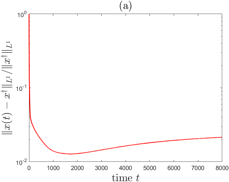
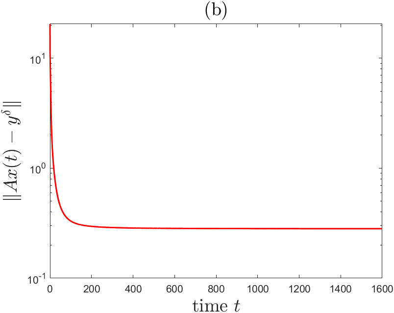
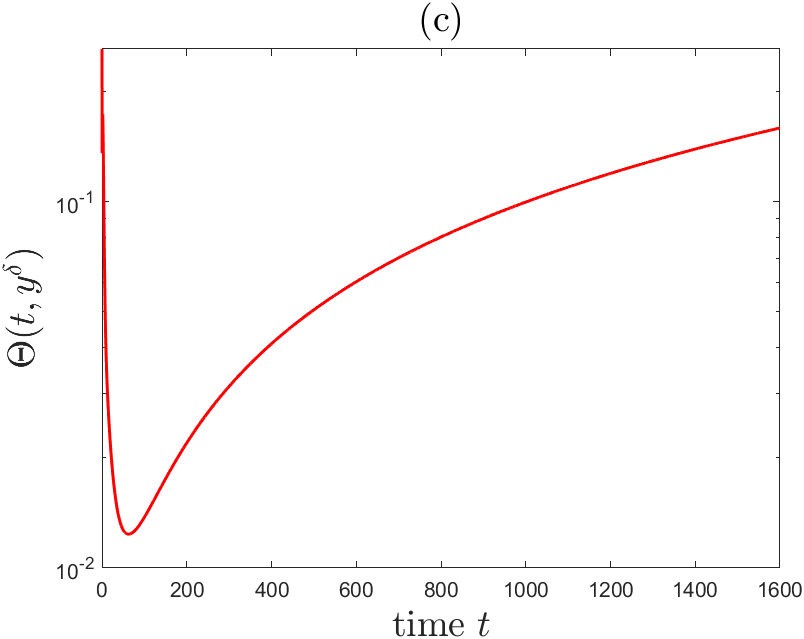
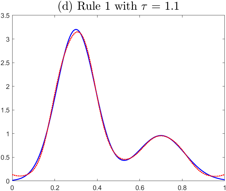
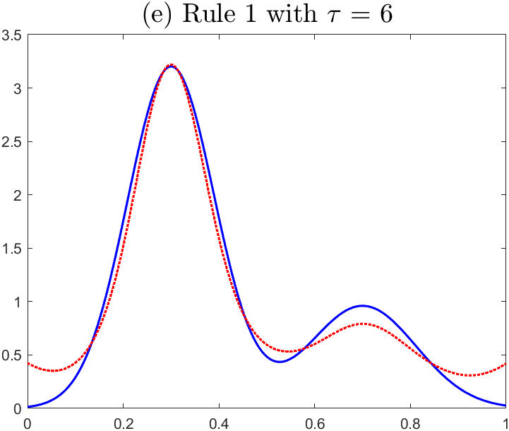
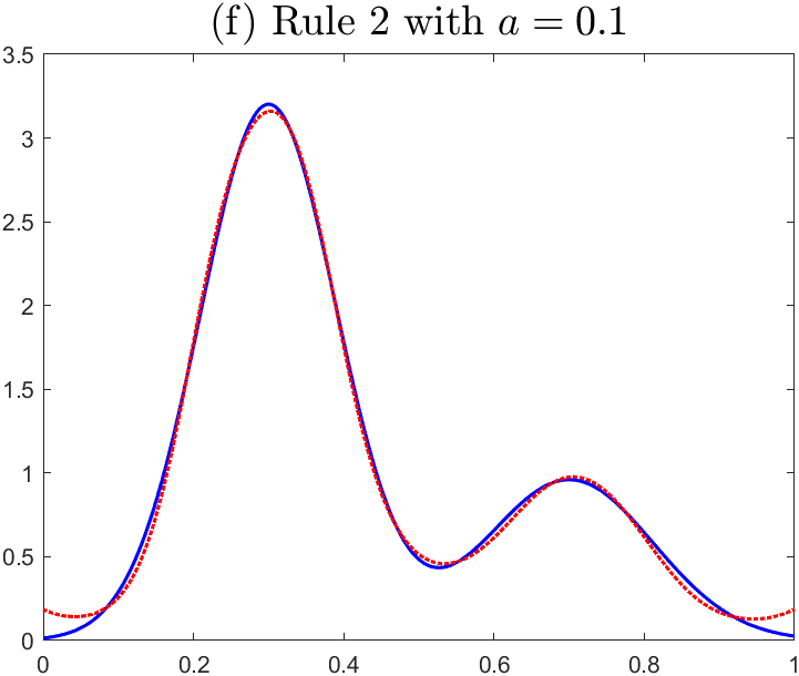
Figure 1. The reconstructed results for Example 3.1 using noisy data with noise level $\delta=0.01$.

In order to visualize the performance of (1.5), in Figure 1 we present the reconstruction results using a noisy data $y^{\delta}$ with the noise level $\delta=0.01$. Figure 1 (a) plots the relative error versus the time which indicates the dual gradient flow (1.5) possesses the semi-convergence property. Figure 1 plots the residual $\|Ax(t)-y^{\delta}\|_{L^{2}}$ versus the time $t$ which demonstrates that Assumption 3 holds with sufficient confidence if the data is corrupted by random noise. Figure 1 (c) plots $\Theta(t,y^{\delta})$ versus $t$ which clearly shows that $t\to\Theta(t,y^{\delta})$ achieves its minimum at a finite number $t>0$. Figure 1 (d)–(f) present the respective reconstruction results $x(t)$ with $t$ chosen by Rule 1 with $\tau=1.1$ and $\tau=6.0$ and by Rule 2 with $a=0.1$.

Example 3.2.

We next consider the computed tomography which consists in determining the density of cross sections of a human body by measuring the attenuation of X-rays as they propagate through the biological tissues. In the numerical simulations we consider test problems that model the standard 2D parallel-beam tomography. We use the full angle model with 45 projection angles evenly distributed between 1 and 180 degrees, with 367 lines per projection. Assuming the sought image is discretized on a $256\times 256$ pixel grid, we may use the function paralleltomo in the MATLAB package AIR TOOLS [19] to discretize the problem. It leads to an ill-conditioned linear algebraic system $Ax=y$, where $A$ is a sparse matrix of size $M\times N$, where $M=16515$ and $N=66536$.

Let the true image be the modified Shepp-Logan phantom of size $256\times 256$ generated by MATLAB. Let $x^{{\dagger}}$ denote the vector formed by stacking all the columns of the true image and let $y=Ax^{\dagger}$ be the true data. We add Gaussian noise on $y$ to generate a noisy data $y^{\delta}$ with relative noise level $\delta_{rel}=\|y^{\delta}-y\|_{2}/\|y\|_{2}$ so that the noise level is $\delta=\delta_{rel}\|y\|_{2}$. We will use $y^{\delta}$ to reconstruct $x^{\dagger}$. In order to capture the feature of the sought image, we take

$$\mathcal{R}(x)=\frac{1}{2\beta}\|x\|_{2}^{2}+|x|_{TV}$$

with a constant $\beta>0$, where $|x|_{TV}$ denotes the total variation of $x$. This $\mathcal{R}$ is strongly convex with $c_{0}=\frac{1}{2\beta}$. The determination of $x=\nabla\mathcal{R}^{*}(A^{*}\lambda)$ for any given $\lambda$ is equivalent to solving the total variation denoising problem

$$x={\rm arg}\min_{z}\left\{\frac{1}{2\beta}\|z-\beta A^{*}\lambda\|_{2}^{2}+|z|_{TV}\right\}$$

which can be solved efficiently by the primal dual hybrid gradient method [3, 41]; we use $\beta=1$ in our computation. With a noisy data $y^{\delta}$ we reconstruct the true image by the dual gradient method (1.5) with $\lambda(0)=0$ which is solved approximately by the 4th Runge-Kutta method (3.1) with constant step-size $\Delta t=0.4\times 10^{-3}$.

Table 2. Numerical results for Example 3.2 by the dual gradient flow (1.5) under Rule 1 and Rule 2.

	Rule 1 with $\tau=1.05$		Rule 1 with $\tau=3.0$		Rule 2 with $a=0.1$
$\delta_{rel}$	$t$	$RE$	$t$	$RE$	$t$	$RE$
5e-2	0.0260	1.9677e-1	0.0144	3.0193e-1	0.0324	1.7331e-1
1e-2	0.1420	6.5240e-2	0.0212	2.2035e-1	0.0992	8.1327e-2
5e-3	0.2640	3.6406e-2	0.0380	1.4581e-1	0.2080	4.5257e-2
1e-3	1.0136	7.3525e-3	0.2160	4.1178e-2	0.6392	1.1537e-2
5e-4	1.7620	3.6169e-3	0.5028	2.1548e-2	1.5904	6.0784e-3

We demonstrate in Table 2 the performance of (1.5) quantitatively by performing the numerical simulations using noisy data with various relative noise levels. We report the value of $t$ determined by Rule 1 with $\tau=1.05$ (proper estimation case) and $\tau=3.0$ (overestimation case) and by Rule 2 with $a=0.1$, we also report the corresponding relative errors $RE:=\|x(t)-x^{\dagger}\|_{2}/\|x^{\dagger}\|_{2}$. The results show that Rule 1 with a proper estimate of the noise level can produce satisfactory reconstruction results; overestimation of noise level can deteriorate the reconstruction accuracy. Rule 2 can produce nice reconstruction results even if it does not rely on the information of noise level.

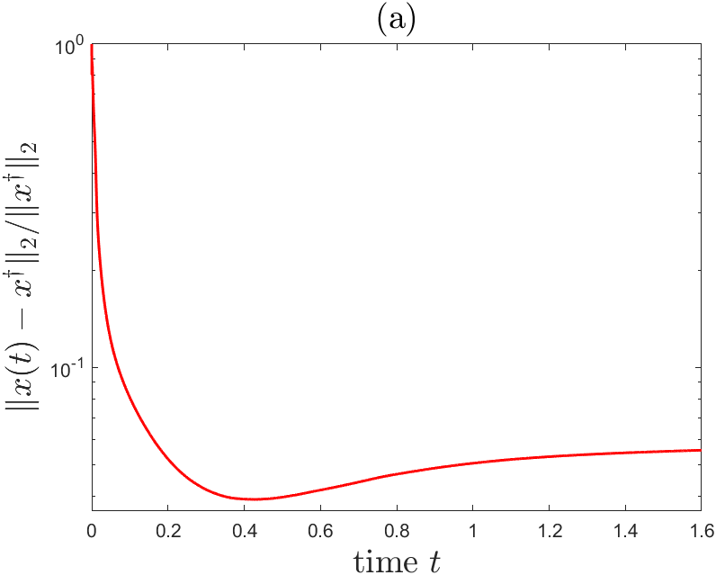
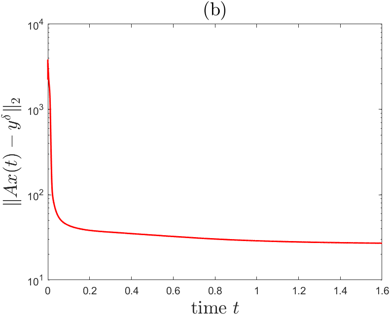
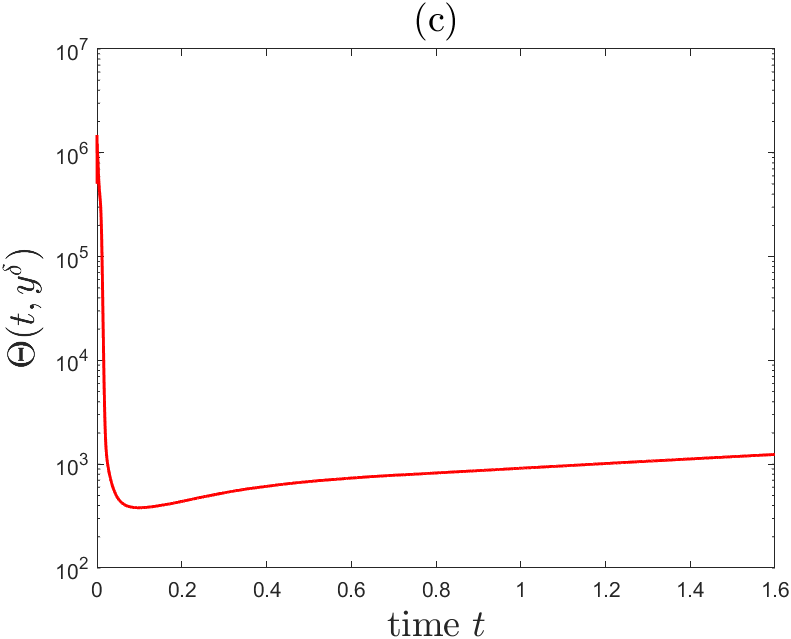
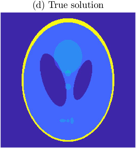
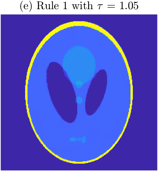
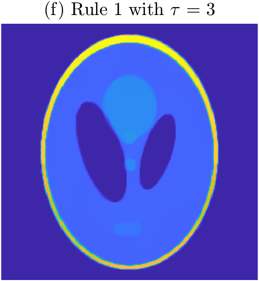
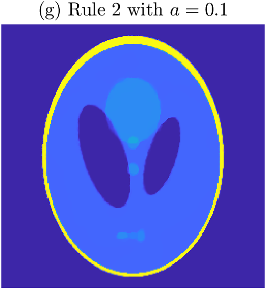
Figure 2. The reconstructed results for Example 3.2 using noisy data with relative noise level $\delta_{rel}=0.01$.

To visualize the performance of (1.5), in Figure 2 we present the reconstruction results using a noisy data $y^{\delta}$ with the relative noise level $\delta_{rel}=0.01$. Figure 2 (a)-(c) plot the relative errors, the residual $\|Ax(t)-y^{\delta}\|_{2}$ and the value of $\Theta(t,y^{\delta})$ versus the time $t$. These results demonstrate the semi-convergence phenomenon of (1.5), the validity of Assumption 3 and well definedness of Rule 2. Figure 2 (d)-(g) plot the true image, the reconstructed images by Rule 1 with $\tau=1.05$ and $\tau=3.0$, and the reconstruction by Rule 2 with $a=0.1$.

Appendix A

Consider (1.2), we want to show that by adding a small multiple of a strongly convex function to $\mathcal{R}$ does not affect the solution too much. Actually, we can prove the following result which is an extension of [10, Theorem 4.4] that proves a special instance related to sparse recovery in finite-dimensional Hilbert spaces.

Proposition A.1.

Let $X$ and $Y$ be Banach space, $A:X\to Y$ a bounded linear operator and $y\in\emph{Ran}(A)$, the range of $A$. Let $\mathcal{R}:X\to(-\infty,\infty]$ be a proper, lower semi-continuous, convex function with $S\cap\emph{dom}(\mathcal{R})\neq\emptyset$, where

$$S:=\arg\min\left\{\mathcal{R}(x):x\in X\mbox{ and }Ax=y\right\}.$$

Assume that $\Psi:X\to(-\infty,\infty]$ is a proper, lower semi-continuous, strongly convex function with $\emph{dom}(\mathcal{R})\subset\emph{dom}(\Psi)$ such that every sublevel set of $\mathcal{R}+\Psi$ is weakly compact. For any $\alpha>0$ define

$$x_{\alpha}:=\arg\min\left\{\mathcal{R}(x)+\alpha\Psi(x):x\in X\mbox{ and }Ax=y\right\}.$$

Then $x_{\alpha}\to x^{*}$ and $\mathcal{R}(x_{\alpha})\to\mathcal{R}(x^{*})$ as $\alpha\to 0$, where $x^{*}\in S$ is such that $\Psi(x^{*})\leq\Psi(x)$ for all $x\in S$.

Proof.

Since $S$ is convex and $\Psi$ is strongly convex, $x_{\alpha}$ and $x^{*}$ are uniquely defined. By the definition of $x_{\alpha}$ and $x^{*}$ we have

$$\mathcal{R}(x_{\alpha})+\alpha\Psi(x_{\alpha})\leq\mathcal{R}(x^{*})+\alpha\Psi(x^{*})$$ (A.1)

and

$$\mathcal{R}(x^{*})\leq\mathcal{R}(x_{\alpha}).$$ (A.2)

Combining these two equations gives

$$\Psi(x_{\alpha})\leq\Psi(x^{*})<\infty.$$ (A.3)

Thus, it follows from (A.1) that $\limsup_{\alpha\to 0}\mathcal{R}(x_{\alpha})\leq\mathcal{R}(x^{*})$ which together with (A.2) shows

$$\lim_{\alpha\to 0}\mathcal{R}(x_{\alpha})=\mathcal{R}(x^{*}).$$ (A.4)

Next we show $x_{\alpha}\to x^{*}$ as $\alpha\to 0$. Since every sublevel set of $\mathcal{R}+\Psi$ is weakly compact, for any sequence $\{\alpha_{k}\}$ with $\alpha_{k}\to 0$, by taking a subsequence if necessary, we may use (A.3) and (A.4) to conclude $x_{\alpha_{k}}\rightharpoonup\hat{x}$ as $k\to\infty$ for some element $\hat{x}\in X$. Since $Ax_{\alpha_{k}}=y$ and $A$ is bounded, letting $k\to\infty$ gives $A\hat{x}=y$. By the weak lower semi-continuity of $\mathcal{R}$ and (A.4) we also have

$$\mathcal{R}(\hat{x})\leq\liminf_{k\to\infty}\mathcal{R}(x_{\alpha_{k}})=\mathcal{R}(x^{*}).$$

Since $x^{*}\in S$, we thus have $\hat{x}\in S$. Consequently $\Psi(x^{*})\leq\Psi(\hat{x})$ by the definition of $x^{*}$. By (A.3) and the weak lower semi-continuity of $\Psi$ we also have

$$\Psi(\hat{x})\leq\liminf_{k\to\infty}\Psi(x_{\alpha_{k}})\leq\limsup_{k\to\infty}\Psi(x_{\alpha_{k}})\leq\Psi(x^{*}).$$ (A.5)

Thus $\hat{x},x^{*}\in S$ and $\Psi(\hat{x})=\Psi(x^{*})$. By uniqueness we must have $\hat{x}=x^{*}$. Consequently $x_{\alpha_{k}}\rightharpoonup x^{*}$ and, by (A.5), $\Psi(x_{\alpha_{k}})\to\Psi(x^{*})$ as $k\to\infty$. Since $\Psi$ is strongly convex, it admits the Kadec property, see [28, Lemma 2.1], which implies $x_{\alpha_{k}}\to x^{*}$ as $k\to\infty$. Since, for any sequence $\{\alpha_{k}\}$ with $\alpha_{k}\to 0$, $\{x_{\alpha_{k}}\}$ has a subsequence converging strongly to $x^{*}$ as $k\to\infty$, we can conclude $x_{\alpha}\to x^{*}$ as $\alpha\to 0$. ∎

References

• [1] U. Amato and W. Hughes, Maximum entropy regularization of Fredholm integral equations of the first kind, Inverse Problems, 7 (1991), 793–808.
• [2] A. B. Bakushinskii, Remarks on choosing a regularization parameter using the quasioptimality and ratio criterion, Comp. Math. Math. Phys., 24 (1984), 181–182.
• [3] S. Bonettini and V. Ruggiero, On the convergence of primal-dual hybrid gradient algorithms for total variation image restoration, J. Math. Imaging Vis., 44 (2012), 236–253.
• [4] J. M. Borwein and C. S. Lewis, Convergence of best entropy estimates, SIAM J. Optim., 1 (1991) 191–205.
• [5] J. M. Borwein and Q. J. Zhu, Techniques of variational analysis, CMS Books in Mathematics/Ouvrages de Mathématiques de la SMC, 20. Springer-Verlag, New York, 2005.
• [6] R. Boţ, G. Dong, P. Elbau and O. Scherzer, Convergence rates of first-and higher-order dynamics for solving linear ill-posed problems, Foundations of Computational Mathematics, 2021 https://doi.org/10.1007/s10208-021-09536-6.
• [7] R. Boţ and T. Hein, Iterative regularization with a geeral penalty term: theory and applications to $L^{1}$ and TV regularization, Inverse Problems, 28 (2012), 104010.
• [8] H. Brezis, Functional Analysis, Sobolev Spaces and Partial Differential Equations, Springer, New York, 2011.
• [9] M. Burger and S. Osher, Convergence rates of convex variational regularization, Inverse Problems 20 (2004), no. 5, 1411–1421.
• [10] J. F. Cai, S. Osher and Z. W. Shen, Linearized Bregman iterations for compressed sensing, Math. Comp., 78 (2009), no. 267, 1515–1536.
• [11] D. H. Chen, D. Jiang, I. Yousept and J. Zou, Variational source conditions for inverse Robin and flux problems by partial measurements, Inverse Probl. Imaging, 16 (2022), no. 2, 283–304.
• [12] P. Deuflhar and F. Bornemann, Scientific Computing with Ordinary Differential Equations, New York: Springer, 2002.
• [13] P. P. B. Eggermont, Maximum entropy regularization for Fredholm integral equations of the first kind, SIAM J. Math. Anal., 24 (1993), no. 6, 1557–1576.
• [14] H. Engl, M. Hanke and A. Neubauer, Regularization of Inverse Problems, New York (NY): Springer, 1996.
• [15] H. Engl and G. Landl, Convergence rates for maximum entropy regularization, SIAM J. Numer. Anal., 30 (1993), 1509–1536.
• [16] J. Flemming, Existence of variational source conditions for nonlinear inverse problems in Banach spaces, J. Inverse Ill-posed Problems, 26 (2018), no. 2, 277–286.
• [17] K. Frick and M. Grasmair, Regularization of linear ill-posed problems by the augmented Lagrangian method and variational inequalities, Inverse Problems, 28 (2012), no. 10, 104005.
• [18] M. Hanke, T. Raus, A general heuristic for choosing the regularization parameter in ill-posed problems, SIAM J. Sci. Comput., 17 (1996), 956–972.
• [19] P. C. Hansen and M. Saxild-Hansen, AIR Tools – a MATLAB package of algebraic iterative reconstruction methods, J. Comput. Appl. Math., 236 (2012), 2167–2178.
• [20] B. Hofmann, B. Kaltenbacher, C. Pöschl and O. Scherzer, A convergence rates result for Tikhonov regularization in Banach spaces with non-smooth operators, Inverse Problems, 23 (2007), 987–1010.
• [21] B. Hofmann and P. Mathé, Parameter choice under variational inequalities, Inverse Problems, 28 (2012), 104006.
• [22] T. Hohage and F. Weidling, Verification of a variational source condition for acoustic inverse medium scattering problems, Inverse Problems 31 (2015), no. 7, 075006.
• [23] T. Hohage and F. Weidling, Characterizations of variational source conditions, converse results, and maxisets of spectral regularization methods, SIAM J. Numer. Anal., 55 (2017), no. 2, 598–620.
• [24] Q. Jin, Hanke-Raus heuristic rule for variational regularization in Banach spaces, Inverse Problems, 32 (2016), 085008.
• [25] Q. Jin, On a heuristic stopping rule for the regularization of inverse problems by the augmented Lagrangian method, Numer. Math., 136 (2017), 973–992.
• [26] Q. Jin, Convergence rates of a dual gradient method for constrained linear ill-posed problems, Numer. Math., 151 (2022), no. 4, 841–871.
• [27] Q. Jin, and W. Wang, Landweber iteration of Kaczmarz type with general non-smooth convex penalty functionals, Inverse Problems, 29 (2013), 085011.
• [28] Q. Jin and M. Zhong, Nonstationary iterated Tikhonov regularization in Banach spaces with uniformly convex penalty terms, Numer. Math., 127 (2014), no. 3, 485–513.
• [29] S. Kindermann and A. Neubauer, On the convergence of the quasioptimality criterion for (iterated) Tikhonov regularization, Inverse Probl. Imaging, 2 (2008), 291–299.
• [30] S. Kindermann and K. Raik, Convergence of heuristic parameter choice rules for convex Tikhonov regularization, SIAM J. Numer. Anal., 58 (2020), no. 3, 1773–1800.
• [31] S. Lu, P. Niu and F. Werner, On the asymptotical regularization for linear inverse problems in presence of white noise, SIAM/ASA J. Uncertain. Quantif., 9 (2021), no. 1, 1–28.
• [32] A. Rieder, Runge-Kutta integrators yield optimal regularization schemes, Inverse Problems, 21 (2005), 453–471.
• [33] F. Schöpfer, A. K. Louis and T. Schuster, Nonlinear iterative methods for linear ill-posed problems in Banach spaces, Inverse problems, 22 (2006), 311–329.
• [34] T. Schuster, B. Kaltenbacher, B. Hofmann and K. S. Kazimierski, Regularization Methods in Banach Spaces, Radon Series on Computational and Applied Mathematics, vol 10, Berlin: Walter de Gruyter, 2012.
• [35] U. Tautenhahn, On the asymptotical regularization of nonlinear ill-posed problems, Inverse Problems 10 (1994), 1405-1418.
• [36] C. Z$\breve{a}$linscu, Convex Analysis in General Vector Spaces, World Scientific Publishing Co., Inc., River Edge, 2002.
• [37] Y. Zhang, B. Hofmann, On fractional asymptotical regularization of linear ill-posed problems in Hilbert spaces, Fract. Calculus. Appl. Anal., 22 (2019), 699-721.
• [38] Y. Zhang and B. Hofmann, On the second-order asymptotical regularization of linear ill-posed inverse problems, Appl. Anal., 99 (2020), no. 6, 1000–1025.
• [39] M. Zhong, W. Wang, S. Tong, An asymptotical regularization with convex constraints for inverse problems, Inverse Problems, 38 (2022), 045007.
• [40] M. Zhong, W. Wang and K. Zhu, On the asymptotical regularization with convex constraints for nonlinear ill-posed problems, Applied Mathematics Letters, 133 (2022), 108247.
• [41] M. Zhu and T. F. Chan, An efficient primal-dual hybrid gradient algorithm for total variation image restoration, CAM Report 08-34, UCLA (2008).