Practical Sketching-Based Randomized Tensor Ring Decomposition

Abstract

Based on sketching techniques, we propose two randomized algorithms for tensor ring (TR) decomposition. Specifically, by defining new tensor products and investigating their properties, we apply the Kronecker sub-sampled randomized Fourier transform and TensorSketch to the alternating least squares problems derived from the minimization problem of TR decomposition to devise the randomized algorithms. From the former, we find an algorithmic framework based on random projection for randomized TR decomposition. Theoretical results on sketch size and complexity analyses for the two algorithms are provided. We compare our proposals with the state-of-the-art method using both synthetic and real data. Numerical results show that they have quite decent performance in accuracy and computing time.

15A69, 68W20

1 Introduction

Tensor decompositions represent a higher-order tensor by multilinear operations over the latent factors, which have found many applications in machine learning, signal processing, chemometrics and so on; see the detailed review in [18, 31, 9]. Two popular decompositions are the Canonical Polyadic (CP) decomposition and the Tucker decomposition. The former has the parameters scaling linearly with the tensor order and the latter is easier to work numerically. So these two decompositions have wide applications [18, 31, 9]. However, they also suffer from some limitations. For example, finding the CP decomposition of a tensor is an NP-hard problem; the number of parameters of Tucker decomposition still scales exponentially with the tensor order. Tensor train (TT) decomposition, which is also known as the matrix product state (MPS) with open boundary conditions in quantum physics [1, 30], came into being to address these challenges [28]. However, it also has some limitations such as the constraint on TT-ranks, the fixed pattern of TT-ranks, and the strict order of TT-cores [35]. For these reasons, Zhao et al. [35] introduced the tensor ring (TR) decomposition, i.e., the MPS with periodic boundary conditions, which has the circular dimensional permutation invariance and hence can overcome some shortcomings of TT decomposition.

Specifically, the TR decomposition in the element-wise form of the tensor $\bm{\mathcal{X}}\in{\mathbb{R}}^{I_{1}\times I_{2}\times\cdots\times I_{N}}$ can be represented as follows:

$$\bm{\mathcal{X}}(i_{1},\cdots,i_{N}) ={\operatorname{trace}}\left({\bf G}_{1}(i_{1}){\bf G}_{2}(i_{2})\cdots{\bf G}_{N}(i_{N})\right)={\operatorname{trace}}\left(\prod_{n=1}^{N}{\bf G}_{n}(i_{n})\right),$$

where ${\bf G}_{n}(i_{n})=\bm{\mathcal{G}}_{n}(:,i_{n},:)\in{\mathbb{R}}^{R_{n}\times R_{n+1}}$ is the $i_{n}$-th lateral slice of the core tensor (TR-core) $\bm{\mathcal{G}}_{n}\in{\mathbb{R}}^{R_{n}\times I_{n}\times R_{n+1}}$. Note that a slice is an 2-order section, i.e., a matrix, of a tensor obtained by fixing all the tensor indices but two, and $R_{N+1}=R_{1}$. The sizes of TR-cores, i.e., $R_{k}$ with $k=1,\cdots,N$, are called TR-ranks. Additionally, we use the notation $\operatorname{TR}\left(\{\bm{\mathcal{G}}_{n}\}_{n=1}^{N}\right)$ to denote the TR decomposition of a tensor. The problem of fitting $\operatorname{TR}\left(\{\bm{\mathcal{G}}_{n}\}_{n=1}^{N}\right)$ to a tensor $\bm{\mathcal{X}}$ can be written as the following minimization problem:

(1) $$\mathop{\arg\min}_{\bm{\mathcal{G}}_{1},\cdots,\bm{\mathcal{G}}_{N}}\|\operatorname{TR}\left(\{\bm{\mathcal{G}}_{n}\}_{n=1}^{N}\right)-\bm{\mathcal{X}}\|_{F},$$

where $\|\cdot\|_{F}$ denotes the Frobenius norm of a matrix or tensor. One of the common approaches to this problem is SVD based, and another one uses the alternating least squares (ALS) [35]. We use the abbreviations TR-SVD and TR-ALS for these two methods in the following text.

Due to the expensive computational costs of the above two methods, it is crucial to design efficient randomized algorithms for computing the TR decompositions of large-scale tensors. As far as we know, the first randomized algorithm for TR decomposition was proposed by Yuan et al. [34] who first applied the randomized Tucker decomposition to the original tensor and then the TR-SVD or TR-ALS to the core tensor of the Tucker decomposition. Finally, the original TR-cores were recovered by combining the factor matrices of the randomized Tucker decomposition and the TR-cores of the core tensor. Later, Ahmadi-Asl et al. [2] summarized some algorithms of TR decomposition and presented several randomized algorithms with randomized SVD. Recently, building on TR-ALS, Malik and Becker [25] provided a sampling method based on leverage scores, which can avoid forming the large coefficient matrices in TR-ALS via the multi-index and can outperform the randomized method given in [34]. Moreover, Malik [21] also provided a new approach to approximate the leverage scores and devised the corresponding sampling algorithm for TR decomposition.

As we know, there are two main types of methods for designing randomized algorithms [13, 10, 26, 14, 33]. One is random sampling, and the other is random projection. The latter is often referred to as the sketching-based method. Actually, both of the two types of methods can be regarded as sketching-based methods because the processed matrix in these two methods can be written in a unified form. That is, the matrix is multiplied by a matrix with random entries. Besides TR decomposition, the above two types of methods have also been applied to other tensor decompositions such as CP, Tucker, and TT decompositions. For example, Battaglino et al. [4] first investigated the uniform sampling for CP decomposition comprehensively, and then Larsen and Kolda [19] considered its leverage-based sampling. The latter inspires the works in [25, 21] on TR decomposition mentioned above. Again, it should be emphasized that the sampling methods used in these works can avoid forming the large coefficient matrices and they carry out sample selection in factor matrices or core tensors. For random projection, scholars mainly used Gaussian random matrix, sub-sampled randomized Hadamard transform (SRHT), sub-sampled randomized Fourier transform (SRFT), CountSketch (CS) and its variant TensorSketch to design the randomized algorithms for CP, Tucker, and TT decompositions; see, e.g., [36, 4, 5, 27, 6, 7, 20]. In particular, in [4], the SRFT is applied to each factor matrix of CP decomposition rather than the large coefficient matrix in the ALS (CP-ALS) derived from the minimization problem of CP decomposition; in [20], the method is mainly built on a formula that combines the TensorSketch and the Kronecker-like form of coefficient matrix.

In this paper, motivated by [25] and the warning in [26, Section 9] that leverage score sampling is rarely a competitive method in practice and may perform markedly worse, we consider the sketching-based methods for TR decomposition on the basis of TR-ALS. Specifically, in our algorithm, we will use Kronecker SRFT (KSRFT), which is similar to what was done in [4] for CP decomposition but with some quite remarkable improvements. This is mainly because unlike the coefficient matrices in CP-ALS [4], it is difficult to straighten the structure of the coefficient matrices in TR-ALS; see Eq. 3 below. To this end, we define a new tensor product and find an elegant property of the product. Moreover, these new findings make us avoid forming the full coefficient matrices, the large sketching matrices and the matrix multiplications between them, and enable us to detect a framework for designing the randomized algorithm for TR decomposition; see Remark 4.2 below for details. Furthermore, as done in [20], we also consider TensorSketch. However, for our problem, it is more complicated. To this end, we define another new product of tensors and obtain a graceful formula. Therefore, in the ideas on sketching methods, the work is mainly inspired by [4] and [20] in essence.

The remainder of this paper is organized as follows. Section 2 provides some preliminaries. In Section 3, we review some existing algorithms for TR decomposition and present our new findings including new tensor products and their properties, structure analysis of the coefficient matrices, and a formula for TensorSketch. The algorithms based on KSRFT and TensorSketch and their theoretical analyses and computational complexities are given in Sections 4 and 5, respectively. In Section 6, we compare our algorithms with the existing ones using both synthetic and real data. Finally, the concluding remarks of the whole paper are presented.

2 Preliminaries

We first introduce some necessary definitions.

Definition 2.1 (Multi-index [12]).

For a positive integer $I$, let $[I]\xlongequal{def}\{1,\cdots,I\}$. For indices $i_{1}\in[I_{1}],\cdots,i_{N}\in[I_{N}]$, a multi-index $i=\overline{i_{1}i_{2}\cdots i_{N}}$ refers to an index which takes all possible combinations of values of the indices, $i_{1},i_{2},\cdots,i_{N}$, for $i_{n}=1,2,\cdots,I_{n}$ with $n=1,2,\cdots,N$ in a specific order. Two common orders are as follows.

1. Little-endian convention (reverse lexicographic ordering)

   $$\overline{i_{1}i_{2}\cdots i_{N}}=i_{1}+(i_{2}-1)I_{1}+(i_{3}-1)I_{1}I_{2}+\cdots+(i_{N}-1)I_{1}\cdots I_{N-1}.$$

2. Big-endian convention (colexicographic ordering)

   $$\overline{i_{1}i_{2}\cdots i_{N}}=i_{N}+(i_{N-1}-1)I_{N}+(i_{N-2}-1)I_{N}I_{N-1}+\cdots+(i_{1}-1)I_{2}\cdots I_{N}.$$

In this paper, unless otherwise stated, we will use the little-endian convention.

Definition 2.2 (Kronecker product).

The Kronecker product of two matrices ${\bf A}=(a_{ij})\in{\mathbb{R}}^{I_{1}\times J_{1}}$ and ${\bf B}\in{\mathbb{R}}^{I_{2}\times J_{2}}$ is a matrix of size $I_{1}I_{2}\times J_{1}J_{2}$ denoted by ${\bf A}\otimes{\bf B}$ and defined as

$${\bf A}\otimes{\bf B}=\begin{bmatrix}a_{11}{\bf B}&\cdots&a_{1J_{1}}{\bf B}\\ \vdots&\ddots&\vdots\\ a_{I_{1}1}{\bf B}&\cdots&a_{I_{1}J_{1}}{\bf B}\end{bmatrix}.$$

If using the notation in Definition 2.1, the element-wise form of the Kronecker product is as follows:

$$({\bf A}\otimes{\bf B})(\overline{i_{2}i_{1}},\overline{j_{2}j_{1}})={\bf A}(i_{1},j_{1}){\bf B}(i_{2},j_{2}).$$

Definition 2.3 (Khatri-Rao product).

The Khatri-Rao product of two matrices ${\bf A}\in{\mathbb{R}}^{I_{1}\times J}$ and ${\bf B}\in{\mathbb{R}}^{I_{2}\times J}$ is a matrix of size $I_{1}I_{2}\times J$ denoted by ${\bf A}\odot{\bf B}$ and defined as

$${\bf A}\odot{\bf B}=[{\bf a}_{1}\otimes{\bf b}_{1},{\bf a}_{2}\otimes{\bf b}_{2},\cdots,{\bf a}_{J}\otimes{\bf b}_{J}],$$

where ${\bf a}_{n}$ and ${\bf b}_{n}$ with $n\in[J]$ are the $n$-th columns of the matrices ${\bf A}$ and ${\bf B}$, respectively.

If using the notation in Definition 2.1, the element-wise form of the Khatri-Rao product is as follows:

$$({\bf A}\odot{\bf B})(\overline{i_{2}i_{1}},j)={\bf A}(i_{1},j){\bf B}(i_{2},j).$$

Definition 2.4 (Mode-$n$ product [8, 18]).

The mode-n product of a tensor $\bm{\mathcal{X}}\in{\mathbb{R}}^{I_{1}\times I_{2}\cdots\times I_{N}}$ with a matrix ${\bf U}\in{\mathbb{R}}^{J\times I_{n}}$ is a tensor of size $I_{1}\times\cdots\times I_{n-1}\times J\times I_{n+1}\times\cdots\times I_{N}$ denoted by $\bm{\mathcal{X}}\times_{n}{\bf U}$ and defined as

$$(\bm{\mathcal{X}}\times_{n}{\bf U})_{i_{1}\cdots i_{n-1}ji_{n+1}\cdots i_{N}}=\sum_{i_{n}=1}^{I_{n}}x_{i_{1}i_{2}\cdots i_{N}}u_{ji_{n}}.$$

Definition 2.5 (Mode-$n$ unfolding [35, 8]).

The mode-n unfolding of a tensor $\bm{\mathcal{X}}\in{\mathbb{R}}^{I_{1}\times I_{2}\cdots\times I_{N}}$ is the matrix ${\bf X}_{[n]}$ of size $I_{n}\times\prod_{j\neq n}I_{j}$ defined element-wise via

$${\bf X}_{[n]}(i_{n},\overline{i_{n+1}\cdots i_{N}i_{1}\cdots i_{n-1}})=\bm{\mathcal{X}}(i_{1},\cdots,i_{N}).$$

Definition 2.6 (Classical mode-$n$ unfolding [35, 8, 18]).

The classical mode-n unfolding of a tensor $\bm{\mathcal{X}}\in{\mathbb{R}}^{I_{1}\times I_{2}\cdots\times I_{N}}$ is the matrix ${\bf X}_{(n)}$ of size $I_{n}\times\prod_{j\neq n}I_{j}$ defined element-wise via

$${\bf X}_{(n)}(i_{n},\overline{i_{1}\cdots i_{n-1}i_{n+1}\cdots i_{N}})=\bm{\mathcal{X}}(i_{1},\cdots,i_{N}).$$

For the tensor in a series of mode-$n$ product form, we can rewrite its mode-$n$ and classical mode-$n$ unfolding matrices using the following formulas.

Proposition 2.7 ([8]).

Let the tensor $\hat{\bm{\mathcal{X}}}$ have the form $\hat{\bm{\mathcal{X}}}=\bm{\mathcal{X}}\times_{1}{\bf U}_{1}\times_{2}{\bf U}_{2}\cdots\times_{N}{\bf U}_{N}$, where $\bm{\mathcal{X}}\in{\mathbb{R}}^{I_{1}\times I_{2}\cdots\times I_{N}}$, and ${\bf U}_{n}\in{\mathbb{R}}^{J_{n}\times I_{n}}$ for $n={1,\cdots,N}$. Then

$$\hat{{\bf X}}_{[n]} ={\bf U}_{n}{\bf X}_{[n]}\left({\bf U}_{n-1}\otimes\cdots\otimes{\bf U}_{1}\otimes{\bf U}_{N}\otimes\cdots\otimes{\bf U}_{n+1}\right)^{\intercal},$$

$$\hat{{\bf X}}_{(n)} ={\bf U}_{n}{\bf X}_{(n)}\left({\bf U}_{N}\otimes\cdots\otimes{\bf U}_{n+1}\otimes{\bf U}_{n-1}\otimes\cdots\otimes{\bf U}_{1}\right)^{\intercal}.$$

Definition 2.8 (Subchain tensor [35]).

Let $\bm{\mathcal{X}}=\operatorname{TR}\left(\{\bm{\mathcal{G}}_{n}\}_{n=1}^{N}\right)\in{\mathbb{R}}^{I_{1}\times I_{2}\cdots\times I_{N}}$. The subchain tensor $\bm{\mathcal{G}}^{\neq n}\in{\mathbb{R}}^{R_{n+1}\times\prod_{j\neq n}I_{j}\times R_{n}}$ is the merging of all TR-cores expect the $n$-th one and can be written slice-wise via

(2) $${\bf G}^{\neq n}(\overline{i_{n+1}\cdots i_{N}i_{1}\cdots i_{n-1}})=\prod_{j=n+1}^{N}{\bf G}_{j}(i_{j})\prod_{j=1}^{n-1}{\bf G}_{j}(i_{j}).$$

In the following, we introduce KSRFT and TensorSketch. As mentioned in Section 1, we will use them to devise the corresponding algorithms.

Definition 2.9 (KSRFT [4, 17]).

The KSRFT is defined as

$$\mathbf{\Phi}=\sqrt{\frac{\prod_{j=1}^{N}I_{j}}{m}}{\bf S}\left(\bigotimes_{j=1}^{N}({\bf F}_{j}{\bf D}_{j})\right),$$

where

• ${\bf S}\in{\mathbb{R}}^{m\times\prod_{j=1}^{N}I_{j}}$ : $m$ rows of the $\prod_{i=j}^{N}I_{j}\times\prod_{j=1}^{N}I_{j}$ identity matrix drawn uniformly at random with replacement from the identity matrix;

• ${\bf F}_{j}\in{\mathbb{C}}^{I_{j}\times I_{j}}$ : (unitary) discrete Fourier transform of dimension $I_{j}$ (also called DFT/FFT matrix);

• ${\bf D}_{j}\in{\mathbb{R}}^{I_{j}\times I_{j}}$ : a diagonal matrix with independent random diagonal entries drawn uniformly from $\{+1,-1\}$ (also called random sign-flip operator).

Remark 2.10.

Actually, the KSRFT is a special Kronecker fast Johnson-Lindenstrauss transform, i.e., KFJLT, proposed and studied in [4, 17, 24].

Definition 2.11 (TensorSketch [29, 11]).

The TensorSketch is defined as $\mathbf{T}=\mathbf{\Omega D}$, where

• $\mathbf{\Omega}\in{\mathbb{R}}^{m\times\prod_{j=1}^{N}I_{j}}$: a matrix with $\mathbf{\Omega}(j,i)=1$ if $j=H(i)$ for all $i\in\left[\prod_{j=1}^{N}I_{j}\right]$ and $\mathbf{\Omega}(j,i)=0$ otherwise;

• $\mathbf{D}\in{\mathbb{R}}^{\prod_{j=1}^{N}I_{j}\times\prod_{i=j}^{N}I_{j}}$: a diagonal matrix with $\mathbf{D}(i,i)=S(i)$.

In the definitions of $\mathbf{\Omega}$ and $\mathbf{D}$,

$$H : [I_{1}]\times[I_{2}]\times\cdots\times[I_{N}]\rightarrow[m]:(i_{1},\ldots,i_{N})\mapsto\left(\sum_{n=1}^{N}(H_{n}(i_{n})-1)\mod m\right)+1,$$

$$S : [I_{1}]\times[I_{2}]\times\cdots\times[I_{N}]\rightarrow\{-1,1\}:(i_{1},\ldots,i_{N})\mapsto\prod_{n=1}^{N}S_{n}(i_{n}),$$

where each $H_{n}$ for $n\in[N]$ is a 3-wise independent hash map that maps $[I_{n}]\rightarrow[m]$, and each $S_{n}$ is a 4-wise independent hash map that maps $[I_{n}]\rightarrow\{-1,1\}$. Recall that a hash map is $k$-wise independent if all the designated $k$ keys are independent random variables.

Remark 2.12.

In Definition 2.11, we use the little-endian convention to compute

$$H(i)=H(\overline{i_{1}i_{2}\cdots i_{N}})\textrm{ and }S(i)=S(\overline{i_{1}i_{2}\cdots i_{N}}),$$

while the definition of the TensorSketch in [11, 23, 22, 20] uses the big-endian convention.

3 Existing algorithms and new findings

We first introduce TR-ALS mentioned in Section 1 and the main idea of the randomized algorithm proposed in [25].

According to Theorem 3.5 in [35], the objective in Eq. 1 can be rewritten as the following $N$ subproblems

(3) $$\mathop{\arg\min}_{{\bf G}_{n(2)}}\|{\bf G}_{[2]}^{\neq n}{\bf G}_{n(2)}^{\intercal}-{\bf X}_{[n]}^{\intercal}\|_{F},\ n=1,\cdots,N.$$

The so-called TR-ALS is a method that keeps all cores fixed except the $n$-th one and finds the solution to the least squares problem Eq. 3 with respect to it. We summarize TR-ALS in Algorithm 1.

Algorithm 1 TR-ALS [35]

1:function $\{\bm{\mathcal{G}}_{n}\}_{n=1}^{N}$= TR-ALS($\bm{\mathcal{X}},R_{1},\cdots,R_{N}$) $\triangleright$ $\bm{\mathcal{X}}$ is the input tensor $\triangleright$ $R_{1},\cdots,R_{N}$ are the TR-ranks

2:    Initialize cores $\bm{\mathcal{G}}_{2},\cdots,\bm{\mathcal{G}}_{N}$

3:    repeat

4:        for $n=1,\cdots,N$ do

5:           Compute ${\bf G}_{[2]}^{\neq n}$ from cores

6:           Update $\bm{\mathcal{G}}_{n}=\mathop{\arg\min}_{\bm{\mathcal{Z}}}\|{\bf G}_{[2]}^{\neq n}{\bf Z}_{(2)}^{\intercal}-{\bf X}_{[n]}^{\intercal}\|_{F}$

7:        end for

8:    until termination criteria met

9:    return $\bm{\mathcal{G}}_{1},\cdots,\bm{\mathcal{G}}_{N}$

10:end function

Since the size of the matrix ${\bf G}_{[2]}^{\neq n}$ is $\prod_{j\neq n}I_{j}\times R_{n}R_{n+1}$, it is very expensive to solve the least squares problem Eq. 3 directly. To tackle this problem, Malik and Becker [25] proposed a random sampling variant of TR-ALS based on importance sampling. The main advantage of the variant is that it can obtain the sketch with sampling without forming the large matrix ${\bf G}_{[2]}^{\neq n}$. This is mainly due to the authors noting that the $\overline{i_{n+1}\cdots i_{N}i_{1}\cdots i_{n-1}}$-th lateral slice of the subchain tensor $\bm{\mathcal{G}}^{\neq n}$ can be given by a sequence of matrix multiplications, that is, Eq. 2 in Definition 2.8. So they devised an algorithm to find the sampled sketch of the tensor $\bm{\mathcal{G}}^{\neq n}$ and hence of the matrix ${\bf G}^{\neq n}_{[2]}$ by extracting $m$ lateral slices from each of the cores $\bm{\mathcal{G}}_{j}$. The algorithm of this sampling method is summarized in Algorithm 2. With this algorithm and the leverage scores or their approximations of the classical mode-$2$ unfolding matrices of TR-cores, the random sampling variant of TR-ALS, i.e., TR-ALS-Sampled, can be derived [25]. We summarize it in Algorithm 3.

Algorithm 2 Sampled Subchain Tensor (SST), summarized from [25]

1:function $\bm{\mathcal{G}}^{\neq n}_{S}$= SST($\texttt{idxs},\bm{\mathcal{G}}_{n+1},\cdots,\bm{\mathcal{G}}_{N},\bm{\mathcal{G}}_{1},\cdots,\bm{\mathcal{G}}_{n-1}$) $\triangleright$ $\bm{\mathcal{G}}_{n}\in{\mathbb{R}}^{R_{n}\times I_{n}\times R_{n+1}},n\in[N]$ $\triangleright$ $\texttt{idxs}\in{\mathbb{R}}^{m\times(N-1)}$ is from the set of tuples $\{i_{n+1}^{(j)},\cdots,i_{N}^{(j)},i_{1}^{(j)},\cdots,i_{n-1}^{(j)}\}$ for $j\in[m]$ $\triangleright$ idxs can be retrieved from the sampling matrix ${\bf S}\in{\mathbb{R}}^{m\times\prod_{k\neq n}I_{k}}$ or the specific sampling with given probabilities

2:    Let $\bm{\mathcal{G}}^{\neq n}_{S}$ be a tensor of size $R_{n+1}\times m\times R_{n}$, where every lateral slice is an $R_{n+1}\times R_{n}$ identity matrix

3:    for $k=n+1,\cdots,N,1,\cdots,n-1$ do

4:        $\bm{\mathcal{G}}_{(k)S}\leftarrow\bm{\mathcal{G}}_{k}(:,\texttt{idxs}(:,k),:)$

5:        $\bm{\mathcal{G}}^{\neq n}_{S}\leftarrow\bm{\mathcal{G}}^{\neq n}_{S}\boxast_{2}\bm{\mathcal{G}}_{(k)S}$ $\triangleright$ we use $\boxast_{2}$ defined in Definition 3.4 below to simplify the representation

6:    end for

7:    return $\bm{\mathcal{G}}^{\neq n}_{S}$

8:end function

Algorithm 3 TR-ALS-Sampled [25]

1:function $\{\bm{\mathcal{G}}_{n}\}_{n=1}^{N}$= TR-ALS-Sampled($\bm{\mathcal{X}},R_{1},\cdots,R_{N},m$) $\triangleright$ $m$ is the sampling size

2:    Initialize cores $\bm{\mathcal{G}}_{2},\cdots,\bm{\mathcal{G}}_{N}$

3:    Compute probability distributions $\bm{p}_{2},\cdots,\bm{p}_{N}$ based on leverage scores

4:    repeat

5:        for $n=1,\cdots,N$ do

6:           Draw sampling matrix $\mathbf{S}$ using the probability distributions of $N-1$ cores

7:           Retrieve idxs from $\mathbf{S}$

8:           $\bm{\mathcal{G}}^{\neq n}_{S}$ = SST($\texttt{idxs},\bm{\mathcal{G}}_{n+1},\cdots,\bm{\mathcal{G}}_{N},\bm{\mathcal{G}}_{1},\cdots,\bm{\mathcal{G}}_{n-1}$)

9:           ${\bf X}_{S[n]}^{\intercal}\leftarrow{\bf S}{\bf X}_{[n]}^{\intercal}$

10:           Update $\bm{\mathcal{G}}_{n}=\mathop{\arg\min}_{\bm{\mathcal{Z}}}\|\hat{{\bf G}}_{S[2]}^{\neq n}{\bf Z}_{(2)}^{\intercal}-\hat{{\bf X}}_{S[n]}^{\intercal}\|_{F}$

11:           Update probability distributions $\bm{p}_{n}$ based on leverage scores

12:        end for

13:    until termination criteria met

14:end function

Motivated by TR-ALS-Sampled and the warning in [26, Section 9], i.e., sampling can be a bit precarious, and inspired by the idea in [4], we would like to combine TR-ALS with the sketching techniques to design the sketching-based algorithms for TR decomposition. To this end, we have to straighten the structure of the matrices ${\mathcal{S}}{\bf G}^{\neq n}_{[2]}$ and ${\bf G}^{\neq n}_{[2]}$, where ${\mathcal{S}}$ is some sketching matrix. This is because, like [4], we also want to find the sketch ${\mathcal{S}}{\bf G}^{\neq n}_{[2]}$ without forming ${\mathcal{S}}$ and ${\bf G}^{\neq n}_{[2]}$. In the following, we present the specific analysis.

Firstly, note that each row of ${\mathcal{S}}{\bf G}^{\neq n}_{[2]}$ is the linear combination of the rows of the matrix ${\bf G}^{\neq n}_{[2]}$, and the rows of the matrix ${\bf G}^{\neq n}_{[2]}$ are the vectorization of the lateral slices of the subchain tensor $\bm{\mathcal{G}}^{\neq n}$. Therefore, from the perspective of the subchain tensor, the above process can be carried out from a linear combination of the lateral slices of $\bm{\mathcal{G}}^{\neq n}$. Moreover, if we use the properties of mode-2 product, the above operation can be written as $\bm{\mathcal{G}}^{\neq n}\times_{2}{\mathcal{S}}$. We illustrate this transformation and process in Figure 1.

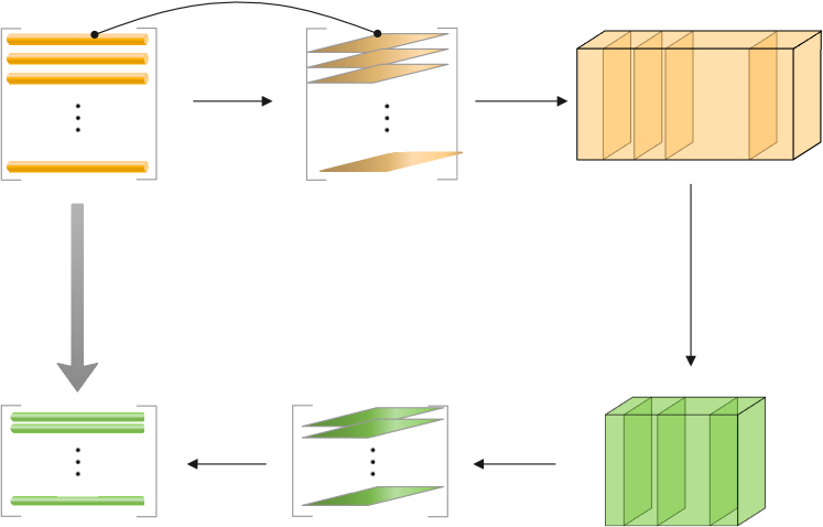
Figure 1: Illustration of the process for obtaining ${\mathcal{S}}{\bf G}^{\neq n}_{[2]}$ via $\bm{\mathcal{G}}^{\neq n}\times_{2}{\mathcal{S}}$.

Secondly, from Eq. 2, we observe that the subchain tensor $\bm{\mathcal{G}}^{\neq n}$ may be written as a Kronecker-like or Khatri-Rao-like product of TR-cores if we define a tensor product felicitously. The product is given as follows, and its graphical illustration is provided in Figure 2a.

Definition 3.1 (Subchain product).

Let $\bm{\mathcal{A}}\in{\mathbb{R}}^{I_{1}\times J_{1}\times K}$ and $\bm{\mathcal{B}}\in{\mathbb{R}}^{K\times J_{2}\times I_{2}}$ be two 3-order tensors, and ${\bf A}(j_{1})$ and ${\bf B}(j_{2})$ be the $j_{1}$-th and $j_{2}$-th lateral slices of $\bm{\mathcal{A}}$ and $\bm{\mathcal{B}}$, respectively. The mode-2 subchain product of $\bm{\mathcal{A}}$ and $\bm{\mathcal{B}}$ is a tensor of size $I_{1}\times J_{1}J_{2}\times I_{2}$ denoted by $\bm{\mathcal{A}}\boxtimes_{2}\bm{\mathcal{B}}$ and defined as

$$(\bm{\mathcal{A}}\boxtimes_{2}\bm{\mathcal{B}})(\overline{j_{1}j_{2}})=\bm{\mathcal{A}}(j_{1})\bm{\mathcal{B}}(j_{2}).$$

That is, with respect to the correspondence on indices, the lateral slices of $\bm{\mathcal{A}}\boxtimes_{2}\bm{\mathcal{B}}$ are the classical matrix products of the lateral slices of $\bm{\mathcal{A}}$ and $\bm{\mathcal{B}}$. The mode-1 and mode-3 subchain products can be defined similarly.

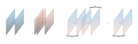
(a) Illustration of the subchain product given in Definition 3.1.

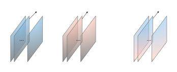
(b) Illustration of the slices-Hadamard product given in Definition 3.4.

Figure 2: Illustration of two new products of 3-order tensors.

Using this definition, we can rewrite the subchain tensor $\bm{\mathcal{G}}^{\neq n}$ in Definition 2.8 as follows

(4) $$\bm{\mathcal{G}}^{\neq n}=\bm{\mathcal{G}}_{n+1}\boxtimes_{2}\cdots\boxtimes_{2}\bm{\mathcal{G}}_{N}\boxtimes_{2}\bm{\mathcal{G}}_{1}\boxtimes_{2}\cdots\boxtimes_{2}\bm{\mathcal{G}}_{n-1}.$$

In the following, we present a property of the above subchain product.

Proposition 3.2.

Let $\bm{\mathcal{A}}\in{\mathbb{R}}^{I_{1}\times J_{1}\times K}$ and $\bm{\mathcal{B}}\in{\mathbb{R}}^{K\times J_{2}\times I_{2}}$ be two 3-order tensors, and ${\bf A}\in{\mathbb{R}}^{R_{1}\times J_{1}}$ and ${\bf B}\in{\mathbb{R}}^{R_{2}\times J_{2}}$ be two matrices. Then

$$(\bm{\mathcal{A}}\times_{2}{\bf A})\boxtimes_{2}(\bm{\mathcal{B}}\times_{2}{\bf B})=(\bm{\mathcal{A}}\boxtimes_{2}\bm{\mathcal{B}})\times_{2}({\bf B}\otimes{\bf A}).$$

Proof 3.3.

By Definitions 2.4, 3.1, and 2.2, upon some computations, we have

$$((\bm{\mathcal{A}}\boxtimes_{2}\bm{\mathcal{B}})\times_{2}({\bf B}\otimes{\bf A}))(i_{1},\overline{r_{1}r_{2}},i_{2})$$

$$=\sum_{\overline{j_{1}j_{2}}=1}^{J_{1}J_{2}}(\bm{\mathcal{A}}\boxtimes_{2}\bm{\mathcal{B}})(i_{1},\overline{j_{1}j_{2}},i_{2})({\bf B}\otimes{\bf A})(\overline{r_{1}r_{2}},\overline{j_{1}j_{2}})$$ by Definition 2.4

$$=\sum_{\overline{j_{1}j_{2}}=1}^{J_{1}J_{2}}\sum_{k=1}^{K}\bm{\mathcal{A}}(i_{1},j_{1},k)\bm{\mathcal{B}}(k,j_{2},i_{2}){\bf B}(r_{2},j_{2}){\bf A}(r_{1},j_{1})$$ by Definitions 3.1 and 2.2

$$=\sum_{k=1}^{K}\sum_{j_{1}=1}^{J_{1}}\bm{\mathcal{A}}(i_{1},j_{1},k){\bf A}(r_{1},j_{1})\sum_{j_{2}=1}^{J_{2}}\bm{\mathcal{B}}(k,j_{2},i_{2}){\bf B}(r_{2},j_{2})$$

$$=\sum_{k=1}^{K}(\bm{\mathcal{A}}\times_{2}{\bf A})(i_{1},r_{1},k)(\bm{\mathcal{B}}\times_{2}{\bf B})(k,r_{2},i_{2})$$ by Definition 2.4

$$=(\bm{\mathcal{A}}\times_{2}{\bf A})\boxtimes_{2}(\bm{\mathcal{B}}\times_{2}{\bf B})(i_{1},\overline{r_{1}r_{2}},i_{2}).$$ by Definition 3.1

Thus, the proof is completed.

Based on the above findings, we can compute ${\mathcal{S}}{\bf G}^{\neq n}_{[2]}$ without forming ${\mathcal{S}}$ and ${\bf G}^{\neq n}_{[2]}$ explicitly by choosing a special ${\mathcal{S}}$. The details are presented in Section 4.

Furthermore, to facilitate the design of the algorithm by TensorSketch as in [20], we define the following product, whose graphical illustration is presented in Figure 2b.

Definition 3.4 (Slices-Hadamard product).

Let $\bm{\mathcal{A}}\in{\mathbb{R}}^{I_{1}\times J\times K}$ and $\bm{\mathcal{B}}\in{\mathbb{R}}^{K\times J\times I_{2}}$ be two 3-order tensors, and ${\bf A}(j)$ and ${\bf B}(j)$ are the $j$-th lateral slices of $\bm{\mathcal{A}}$ and $\bm{\mathcal{B}}$, respectively. The mode-2 slices-Hadamard product of $\bm{\mathcal{A}}$ and $\bm{\mathcal{B}}$ is a tensor of size $I_{1}\times J\times I_{2}$ denoted by $\bm{\mathcal{A}}\boxast_{2}\bm{\mathcal{B}}$ and defined as

$$(\bm{\mathcal{A}}\boxast_{2}\bm{\mathcal{B}})(j)=\bm{\mathcal{A}}(j)\bm{\mathcal{B}}(j).$$

That is, the $j$-th lateral slice of $\bm{\mathcal{A}}\boxast_{2}\bm{\mathcal{B}}$ is the classical matrix product of the $j$-th lateral slices of $\bm{\mathcal{A}}$ and $\bm{\mathcal{B}}$. The mode-1 and mode-3 slices-Hadamard product can be defined similarly.

Using Definition 2.2, similar to the proof of Proposition 3.2, we can prove the following result.

Proposition 3.5.

Let $\bm{\mathcal{A}}\in{\mathbb{R}}^{I_{1}\times J_{1}\times K}$ and $\bm{\mathcal{B}}\in{\mathbb{R}}^{K\times J_{2}\times I_{2}}$ be two 3-order tensors, and ${\bf A}\in{\mathbb{R}}^{M\times J_{1}}$ and ${\bf B}\in{\mathbb{R}}^{M\times J_{2}}$ be two matrices. Then

$$(\bm{\mathcal{A}}\times_{2}{\bf A})\boxast_{2}(\bm{\mathcal{B}}\times_{2}{\bf B})=(\bm{\mathcal{A}}\boxtimes_{2}\bm{\mathcal{B}})\times_{2}({\bf B}^{\intercal}\odot{\bf A}^{\intercal})^{\intercal}.$$

With the slices-Hadamard product, we have the following formula which can avoid forming the TensorSketch and implementing the matrix multiplication between large matrices.

Proposition 3.6.

Let ${\bf S}_{n}=\mathbf{\Omega}_{n}{\bf D}_{n}\in{\mathbb{R}}^{m\times I_{n}}$, where $\mathbf{\Omega}_{n}\in{\mathbb{R}}^{m\times I_{n}}$ and ${\bf D}_{n}\in{\mathbb{R}}^{I_{n}\times I_{n}}$ are defined based on $H_{n}$ and $S_{n}$ in Definition 2.11, respectively. Let ${\bf T}\in{\mathbb{R}}^{m\times\prod_{j=1}^{N}I_{N}}$ be defined in Definition 2.11 and $\bm{\mathcal{P}}=\bm{\mathcal{A}}^{(1)}\boxtimes_{2}\bm{\mathcal{A}}^{(2)}\boxtimes_{2}\cdots\boxtimes_{2}\bm{\mathcal{A}}^{(N)}$ with $\bm{\mathcal{A}}^{(n)}\in{\mathbb{R}}^{R_{n}\times I_{n}\times R_{n+1}}$ for $n\in[N]$. Then

$$\bm{\mathcal{P}}\times_{2}{\bf T}=\operatorname{FFT}^{-1}\left(\boxast_{2~{}n=1}^{~{}~{}N}\operatorname{FFT}\left(\bm{\mathcal{A}}^{(n)}\times_{2}\mathbf{S}_{n},[~{}],2\right),[~{}],2\right).$$

Proof 3.7.

For simplicity, we only present the proof for $N=2$ here. Extending the proof to the general case is immediate.

On the one hand, the mode-$2$ products of $\bm{\mathcal{A}}^{(1)}$ with ${\bf S}_{1}$ and of $\bm{\mathcal{A}}^{(2)}$ with ${\bf S}_{2}$ can be represented by the following two $m-1$ degree matrix polynomials

$${\mathcal{P}}^{(1)}(\omega) =\sum_{i_{1}=1}^{I_{1}}S_{1}(i_{1})\bm{\mathcal{A}}^{(1)}(:,i_{1},:)\omega^{H_{1}(i_{1})-1}=\sum_{m^{\prime}=1}^{m}c^{(1)}_{m^{\prime}}\omega^{m^{\prime}-1}\in{\mathbb{R}}^{R_{1}\times R_{2}},$$

$${\mathcal{P}}^{(2)}(\omega) =\sum_{i_{2}=1}^{I_{2}}S_{2}(i_{2})\bm{\mathcal{A}}^{(2)}(:,i_{2},:)\omega^{H_{2}(i_{2})-1}=\sum_{m^{\prime}=1}^{m}c^{(2)}_{m^{\prime}}\omega^{m^{\prime}-1}\in{\mathbb{R}}^{R_{2}\times R_{3}},$$

where $c^{(1)}_{1},\ldots,c^{(1)}_{m}\in{\mathbb{R}}^{R_{1}\times R_{2}}$ and $c^{(2)}_{1},\ldots,c^{(2)}_{m}\in{\mathbb{R}}^{R_{2}\times R_{3}}$ are coefficient matrices, and $\omega$ satisfies $\omega^{m}=1$ but $\omega^{m^{\prime}}\neq 1$ for $m^{\prime}=1,\ldots,m-1$.

On the other hand, $\bm{\mathcal{P}}\times_{2}\mathbf{T}$ can be represented as the following matrix polynomial

(6) $${\mathcal{P}}(\omega) =\sum_{i=1}^{I_{1}I_{2}}S(i)\bm{\mathcal{P}}(:,i,:)\omega^{H(i)-1}=\sum_{m^{\prime}=1}^{m}c_{m^{\prime}}\omega^{m^{\prime}-1}\in{\mathbb{R}}^{R_{1}\times R_{3}},$$

where $c_{1},\ldots,c_{m}\in{\mathbb{R}}^{R_{1}\times R_{3}}$ are coefficient matrices, $i=\overline{i_{1}i_{2}}$ and $\omega$ satisfies the constraints mentioned above.

Note that $\bm{\mathcal{P}}=\bm{\mathcal{A}}^{(1)}\boxtimes_{2}\bm{\mathcal{A}}^{(2)}\in{\mathbb{R}}^{R_{1}\times I_{1}I_{2}\times R_{3}}$ with $\bm{\mathcal{A}}^{(n)}\in{\mathbb{R}}^{R_{n}\times I_{n}\times R_{n+1}}$ for $n=1,2$. Then, according to Definition 3.1, we have

(7) $$\bm{\mathcal{P}}(:,i,:)=\bm{\mathcal{A}}^{(1)}(:,i_{1},:)\bm{\mathcal{A}}^{(2)}(:,i_{2},:),$$

where $i\in[I_{1}I_{2}]$, $i_{1}\in[I_{1}]$, and $i_{2}\in[I_{2}]$. Substituting Eq. 7 into Eq. 6 implies

$${\mathcal{P}}(\omega) =\sum_{\overline{i_{1}i_{2}}=1}^{I_{1}I_{2}}S(\overline{i_{1}i_{2}})\bm{\mathcal{A}}^{(1)}(:,i_{1},:)\bm{\mathcal{A}}^{(2)}(:,i_{2},:)\omega^{H(\overline{i_{1}i_{2}})-1},$$

which together with Definition 2.11 and the constraints on $\omega$ mentioned above gives

$${\mathcal{P}}(\omega) =\sum_{i_{1}=1}^{I_{1}}\sum_{i_{2}=1}^{I_{2}}S_{1}(i_{1})S_{2}(i_{2})\bm{\mathcal{A}}^{(1)}(:,i_{1},:)\bm{\mathcal{A}}^{(2)}(:,i_{2},:)\omega^{H_{1}(i_{1})+H_{2}(i_{2})-2~{}mod~{}m}$$

$$=\sum_{i_{1}=1}^{I_{1}}S_{1}(i_{1})\bm{\mathcal{A}}^{(1)}(:,i_{1},:)\omega^{H_{1}(i_{1})-1}\sum_{i_{2}=1}^{I_{2}}S_{2}(i_{2})\bm{\mathcal{A}}^{(2)}(:,i_{2},:)\omega^{H_{2}(i_{2})-1}$$

(8) $$={\mathcal{P}}^{(1)}(\omega){\mathcal{P}}^{(2)}(\omega).$$

Thus, viewing

$$c_{1},\cdots,c_{m};~{}\ c_{1}^{(1)},\cdots,c_{m}^{(1)};~{}\ c_{1}^{(2)},\cdots,c_{m}^{(2)}$$

as the lateral slices of the tensors $\bm{\mathcal{C}},\bm{\mathcal{C}}^{(1)}$, and $\bm{\mathcal{C}}^{(2)}$, respectively, according to the famous convolution theorem, we can see that 3.7 can be represented as

$$\bm{\mathcal{C}}=\operatorname{FFT}^{-1}\left(\operatorname{FFT}(\bm{\mathcal{C}}^{(1)},[~{}],2)\boxast_{2}\operatorname{FFT}(\bm{\mathcal{C}}^{(2)},[~{}],2),[~{}],2\right).$$

More precisely, we have

$$\bm{\mathcal{P}}\times_{2}{\bf T}=\operatorname{FFT}^{-1}\left(\operatorname{FFT}\left(\bm{\mathcal{A}}^{(1)}\times_{2}\mathbf{S}_{1},[~{}],2\right)\boxast_{2}\operatorname{FFT}\left(\bm{\mathcal{A}}^{(2)}\times_{2}\mathbf{S}_{2},[~{}],2\right),[~{}],2\right).$$

This is the desired result.

4 KSRFT-based randomized TR decomposition

In this section, we present the randomized algorithm of TR decomposition based on KSRFT and discuss its theoretical analysis and computational complexity.

4.1 Algorithms

According to the analyses in Section 3 and inspired by [4], we choose ${\mathcal{S}}\in{\mathbb{R}}^{m\times\prod_{j\neq n}I_{j}}$ as

(9) $${\mathcal{S}}={\bf S}{\bf F}{\bf D},$$

where ${\bf F}=\bigotimes_{\begin{subarray}{c}n-1,\cdots,1,\\ N,\cdots,n+1\end{subarray}}{\bf F}_{j}$ and ${\bf D}=\bigotimes_{\begin{subarray}{c}n-1,\cdots,1,\\ N,\cdots,n+1\end{subarray}}{\bf D}_{j}$ with ${\bf F}_{j}\in{\mathbb{R}}^{I_{j}\times I_{j}}$ and ${\bf D}_{j}\in{\mathbb{R}}^{I_{j}\times I_{j}}$ being defined in Definition 2.9, and the meaning of ${\bf S}$ will be clarified later. Thus, the reduced problem of Eq. 3 is

(10) $$\mathop{\arg\min}_{{\bf G}_{n(2)}}\left\|{\bf S}{\bf F}{\bf D}{\bf G}_{[2]}^{\neq n}{\bf G}_{n(2)}^{\intercal}-{\bf S}{\bf F}{\bf D}{\bf X}_{[n]}^{\intercal}\right\|_{F}.$$

From the discussions in Section 3, we know that finding ${\bf F}{\bf D}{\bf G}_{[2]}^{\neq n}$ can be transformed into finding $\bm{\mathcal{G}}^{\neq n}\times_{2}({\bf F}{\bf D})$. While, using Eq. 4 and Proposition 3.2, we have

(11) $$\hat{\bm{\mathcal{G}}}^{\neq n} =\bm{\mathcal{G}}^{\neq n}\times_{2}({\bf F}{\bf D})=\bm{\mathcal{G}}^{\neq n}\times_{2}\left(\left(\bigotimes_{\begin{subarray}{c}n-1,\cdots,1,\\ N,\cdots,n+1\end{subarray}}{\bf F}_{j}\right)\left(\bigotimes_{\begin{subarray}{c}n-1,\cdots,1,\\ N,\cdots,n+1\end{subarray}}{\bf D}_{j}\right)\right)$$

$$=(\bm{\mathcal{G}}_{n+1}\times_{2}({\bf F}_{n+1}{\bf D}_{n+1}))\boxtimes_{2}\cdots\boxtimes_{2}(\bm{\mathcal{G}}_{N}\times_{2}({\bf F}_{N}{\bf D}_{N}))$$

$$\quad\quad\boxtimes_{2}(\bm{\mathcal{G}}_{1}\times_{2}({\bf F}_{1}{\bf D}_{1}))\boxtimes_{2}\cdots\boxtimes_{2}(\bm{\mathcal{G}}_{n-1}\times_{2}({\bf F}_{n-1}{\bf D}_{n-1})).$$

As a result,

$${\bf F}{\bf D}{\bf G}_{[2]}^{\neq n}=\hat{\bf G}_{[2]}^{\neq n}.$$

Thus, by mixing the lateral slices of each core $\bm{\mathcal{G}}_{j}$ via the small matrices ${\bf F}_{j}$ and ${\bf D}_{j}$, we get ${\bf F}{\bf D}{\bf G}_{[2]}^{\neq n}$, which can avoid forming the large matrices ${\bf F}$, ${\bf D}$, and ${\bf G}^{\neq n}_{[2]}$ explicitly.

Note that the second term in Eq. 10 is equivalent to

$${\bf S}\hat{{\bf X}}_{[n]}^{\intercal}({\bf D}_{n}{\bf F}_{n}^{*})^{\intercal},$$

where $\hat{\bm{\mathcal{X}}}=\bm{\mathcal{X}}\times_{1}({\bf F}_{1}{\bf D}_{1})\times_{2}({\bf F}_{2}{\bf D}_{2})\cdots\times_{N}({\bf F}_{N}{\bf D}_{N})$, i.e., $\hat{\bf X}_{[n]}={\bf F}_{n}{\bf D}_{n}{\bf X}_{[n]}(({\bf F}_{n-1}{\bf D}_{n-1})\otimes\cdots\otimes({\bf F}_{1}{\bf D}_{1})\otimes({\bf F}_{N}{\bf D}_{N})\otimes\cdots\otimes({\bf F}_{n+1}{\bf D}_{n+1}))^{\intercal}$, and the superscript “$*$” denotes the conjugate transpose. As explained in [4], using the within the loop body and hence can significantly improve the computational efficiency.

Thus, our reduced problem has the following form

(12) $$\mathop{\arg\min}_{{\bf G}_{n(2)}}\|\left({\bf S}\hat{{\bf G}}_{[2]}^{\neq n}\right){\bf G}_{n(2)}^{\intercal}-{\bf S}\hat{{\bf X}}_{[n]}^{\intercal}\left({\bf D}_{n}{\bf F}_{n}^{*}\right)^{\intercal}\|_{F}.$$

To avoid sampling the rows of $\hat{\bf G}^{\neq n}_{[2]}$, i.e., the lateral slices of the large mixed subchain tensor $\hat{\bm{\mathcal{G}}}^{\neq n}$ directly, we use the sampling strategy in Algorithm 2. That is, we sample the lateral slices of the $N-1$ cores individually and then form the sampled mixed subchain tensor $\hat{\bm{\mathcal{G}}}^{\neq n}\times_{2}{\bf S}$. This process can be expressed as follows:

(13) $$\hat{\bm{\mathcal{G}}}^{\neq n}\times_{2}{\bf S} =((\bm{\mathcal{G}}_{n+1}\times_{2}({\bf F}_{n+1}{\bf D}_{n+1}))\boxtimes_{2}\cdots\boxtimes_{2}(\bm{\mathcal{G}}_{N}\times_{2}({\bf F}_{N}{\bf D}_{N}))$$

$$\quad\quad\boxtimes_{2}(\bm{\mathcal{G}}_{1}\times_{2}({\bf F}_{1}{\bf D}_{1}))\boxtimes_{2}\cdots\boxtimes_{2}(\bm{\mathcal{G}}_{n-1}\times_{2}({\bf F}_{n-1}{\bf D}_{n-1})))\times_{2}{\bf S}$$

$$=(\bm{\mathcal{G}}_{n+1}\times_{2}({\bf S}_{n+1}{\bf F}_{n+1}{\bf D}_{n+1}))\boxast_{2}\cdots\boxast_{2}(\bm{\mathcal{G}}_{N}\times_{2}({\bf S}_{N}{\bf F}_{N}{\bf D}_{N}))$$

$$\quad\quad\boxast_{2}(\bm{\mathcal{G}}_{1}\times_{2}({\bf S}_{1}{\bf F}_{1}{\bf D}_{1}))\boxast_{2}\cdots\boxast_{2}(\bm{\mathcal{G}}_{n-1}\times_{2}({\bf S}_{n-1}{\bf F}_{n-1}{\bf D}_{n-1})),$$

where ${\bf S}_{j}\in{\mathbb{R}}^{m\times I_{j}}$ is the sampling matrix for the $j$-th core. According to Proposition 3.5, we can see that ${\bf S}=\left(\bigodot_{\begin{subarray}{c}n-1,\cdots,1,\\ N,\cdots,n+1\end{subarray}}{\bf S}_{j}^{\intercal}\right)^{\intercal}$. Thus, using the property of Khatri-Rao product, we have

(14) $${\mathcal{S}}=\left(\bigodot_{\begin{subarray}{c}n-1,\cdots,1,\\ N,\cdots,n+1\end{subarray}}{\bf S}_{j}^{\intercal}\right)^{\intercal}\left(\bigotimes_{\begin{subarray}{c}n-1,\cdots,1,\\ N,\cdots,n+1\end{subarray}}({\bf F}_{j}{\bf D}_{j})\right)=\left(\bigodot_{\begin{subarray}{c}n-1,\cdots,1,\\ N,\cdots,n+1\end{subarray}}({\bf S}_{j}{\bf F}_{j}{\bf D}_{j})^{\intercal}\right)^{\intercal},$$

and hence we can also call it the Khatri-Rao SRFT. Note that the ${\mathcal{S}}$ used in [4] has the same structure as ${\mathcal{S}}$ in Eq. 14 though the structure was not provided explicitly there.

The above discussions imply Algorithm 4.

Algorithm 4 TR-KSRFT-ALS (Proposal)

1:function $\{\bm{\mathcal{G}}_{n}\}_{n=1}^{N}$= TR-KSRFT-ALS($\bm{\mathcal{X}},R_{1},\cdots,R_{N},m$) $\triangleright$ $\bm{\mathcal{G}}_{n}\in{\mathbb{R}}^{R_{n}\times I_{n}\times R_{n+1}},n\in[N]$; $\bm{\mathcal{X}}\in{\mathbb{R}}^{I_{1}\times\cdots\times I_{N}}$ $\triangleright$ $R_{1},\cdots,R_{N}$ are the TR-ranks $\triangleright$ $m$ is the uniform sampling size

2:    Initialize cores ${\bm{\mathcal{G}}}_{2},\cdots,{\bm{\mathcal{G}}}_{N}$

3:    Define random sign-flip operators ${\bf D}_{j}$ and FFT matrices ${\bf F}_{j}$, for $j\in[N]$

4:    Mix cores: $\hat{\bm{\mathcal{G}}}_{n}\leftarrow\bm{\mathcal{G}}_{n}\times_{2}({\bf F}_{n}{\bf D}_{n})$, for $n={2,\cdots,N}$

5:    Mix tensor: $\hat{\bm{\mathcal{X}}}\leftarrow\bm{\mathcal{X}}\times_{1}({\bf F}_{1}{\bf D}_{1})\times_{2}({\bf F}_{2}{\bf D}_{2})\cdots\times_{N}({\bf F}_{N}{\bf D}_{N})$

6:    repeat

7:        for $n=1,\cdots,N$ do

8:           Define sampling operator ${\bf S}\in{\mathbb{R}}^{m\times\prod_{j\neq n}I_{j}}$

9:           Retrieve idxs from ${\bf S}$

10:           $\hat{\bm{\mathcal{G}}}^{\neq n}_{S}$ = SST($\texttt{idxs},\hat{\bm{\mathcal{G}}}_{n+1},\cdots,\hat{\bm{\mathcal{G}}}_{N},\hat{\bm{\mathcal{G}}}_{1},\cdots,\hat{\bm{\mathcal{G}}}_{n-1}$)

11:           $\hat{{\bf X}}_{S[n]}^{\intercal}\leftarrow{\bf S}\hat{{\bf X}}_{[n]}^{\intercal}\left({\bf D}_{n}{\bf F}_{n}^{*}\right)^{\intercal}$

12:           Update $\bm{\mathcal{G}}_{n}=\mathop{\arg\min}_{\bm{\mathcal{Z}}}\|\hat{{\bf G}}_{S[2]}^{\neq n}{\bf Z}_{(2)}^{\intercal}-\hat{{\bf X}}_{S[n]}^{\intercal}\|_{F}$ subject to $\bm{\mathcal{G}}_{n}$ being real-valued

13:           $\hat{\bm{\mathcal{G}}}_{n}\leftarrow\bm{\mathcal{G}}_{n}\times_{2}({\bf F}_{n}{\bf D}_{n})$

14:        end for

15:    until termination criteria met

16:    return $\bm{\mathcal{G}}_{1},\cdots,\bm{\mathcal{G}}_{N}$

17:end function

Furthermore, note that, with the property of the Frobenius norm, the reduced problem Eq. 12 can be rewritten as

$$\mathop{\arg\min}_{{\bf G}_{n(2)}}\|\left({\bf S}\hat{{\bf G}}_{[2]}^{\neq n}\right){\bf G}_{n(2)}^{\intercal}\left({\bf F}_{n}{\bf D}_{n}\right)^{\intercal}-{\bf S}\hat{{\bf X}}_{[n]}^{\intercal}\|_{F}.$$

Thus, setting $\hat{\bf G}_{n(2)}={\bf F}_{n}{\bf D}_{n}{\bf G}_{n(2)}$, we have

(15) $$\mathop{\arg\min}_{\hat{\bf G}_{n(2)}}\|\left({\bf S}\hat{{\bf G}}_{[2]}^{\neq n}\right)\hat{\bf G}_{n(2)}^{\intercal}-\left({\bf S}\hat{{\bf X}}_{[n]}^{\intercal}\right)\|_{F}.$$

Consequently, we can solve the above problem to get $\hat{\bm{\mathcal{G}}}_{n}$ first and then recover the original core $\bm{\mathcal{G}}_{n}$ from it. The specific algorithm is summarized in Algorithm 5.

Algorithm 5 TR-KSRFT-ALS-Premix (Proposal)

1:function $\{\bm{\mathcal{G}}_{n}\}_{n=1}^{N}$= TR-KSRFT-ALS-Premix($\bm{\mathcal{X}},R_{1},\cdots,R_{N},m$) $\triangleright$ $\bm{\mathcal{G}}_{n}\in{\mathbb{C}}^{R_{n}\times I_{n}\times R_{n+1}},n\in[N]$; $\bm{\mathcal{X}}\in{\mathbb{C}}^{I_{1}\times\cdots\times I_{N}}$ $\triangleright$ $R_{1},\cdots,R_{N}$ are the TR-ranks $\triangleright$ $m$ is the uniform sampling size

2:    Define random sign-flip operators ${\bf D}_{j}$ and FFT matrices ${\bf F}_{j}$, for $j\in[N]$

3:    Mix tensor: $\hat{\bm{\mathcal{X}}}\leftarrow\bm{\mathcal{X}}\times_{1}({\bf F}_{1}{\bf D}_{1})\times_{2}({\bf F}_{2}{\bf D}_{2})\cdots\times_{N}({\bf F}_{N}{\bf D}_{N})$

4:    Initialize cores $\hat{\bm{\mathcal{G}}}_{2},\cdots,\hat{\bm{\mathcal{G}}}_{N}$

5:    repeat

6:        for $n=1,\cdots,N$ do

7:           Define sampling operator ${\bf S}\in{\mathbb{R}}^{m\times\prod_{j\neq n}I_{j}}$

8:           Retrieve idxs from ${\bf S}$

9:           $\hat{\bm{\mathcal{G}}}^{\neq n}_{S}$ = SST($\texttt{idxs},\hat{\bm{\mathcal{G}}}_{n+1},\cdots,\hat{\bm{\mathcal{G}}}_{N},\hat{\bm{\mathcal{G}}}_{1},\cdots,\hat{\bm{\mathcal{G}}}_{n-1}$)

10:           $\hat{{\bf X}}_{S[n]}^{\intercal}\leftarrow{\bf S}\hat{{\bf X}}_{[n]}^{\intercal}$

11:           Update $\hat{\bm{\mathcal{G}}}_{n}=\mathop{\arg\min}_{\bm{\mathcal{Z}}}\|\hat{{\bf G}}_{S[2]}^{\neq n}{\bf Z}_{(2)}^{\intercal}-\hat{{\bf X}}_{S[n]}^{\intercal}\|_{F}$

12:        end for

13:    until termination criteria met

14:    for $n=1,\cdots,N$ do

15:        Unmix cores: $\bm{\mathcal{G}}_{n}\leftarrow\hat{\bm{\mathcal{G}}}_{n}\times_{2}({\bf D}_{n}{\bf F}_{n}^{*})$

16:    end for

17:    return $\bm{\mathcal{G}}_{1},\cdots,\bm{\mathcal{G}}_{N}$

18:end function

Remark 4.1.

Algorithms 4 and 5 are inspired by [4], which designed some practical randomized algorithms for CP decomposition. One of our main contributions is that we present an elegant way to transform the problem Eq. 3 to the problem Eq. 12 with the new tensor product and its property. This allows us to design algorithms as elegantly as in [4]. Compared with the method in [25], which is mainly inspired by the work in [19], our method may work better for some special data, such as for the data whose TR-cores include outliers [16, 15]. This is mainly because, with the sampling method in Algorithm 2, TR-ALS-Sampled may sample the aforementioned outliers with high probability many times and hence may cause an unstable result. Although we also use Algorithm 2, the sampling in our method is uniform sampling and the tensor is transformed by the randomized Fourier transform before sampling. The above analysis is supported by the numerical results of the third experiment on synthetic data in Section 6.

Remark 4.2.

Upon close examination of the derivation of Algorithm 4, we may let ${\bf F}_{j}{\bf D}_{j}$ be any suitable randomized matrices. For example, we can set them to be the CountSketch matrices for sparse input data. The corresponding method can be denoted by TR-CS-ALS. Moreover, we are surprised to find that if we set them to be the transpose of the factor matrices appearing in the randomized Tucker decomposition, we can recover the algorithm rTR-ALS proposed in [34]. These analyses present an affirmative result that reducing the dimension of each mode of the original tensor with a suitable sketching matrix, finding the TR decomposition of the reduced tensor, and then recovering the TR decomposition of the original tensor is feasible. Note that, in these cases, the step on sampling is not necessary and hence the final product is the subchain product as in Eq. 11 but not the slices-Hadamard product as in Eq. 13. The differences are illustrated in Figure 3, from which we can also find that the sketching-based methods for TR decomposition can be mainly classified into two classes: one is based on the subchain product, and the other is based on the slices-Hadamard product. We also summarize all the algorithms mentioned above in Table 1.

Table 1: Comparisons of randomized algorithms for TR decomposition

Algorithms	${\bf S}_{j}$ in Figure 3	${\mathcal{S}}$ in Figure 3	Product
rTR-ALS ([34])	${\bf Q}_{j}^{\intercal}$ from the QR decomposition of ${\bf X}_{[j]}{\bf M}$ with ${\bf M}$ being a Gaussian matrix	$\bigotimes_{\begin{subarray}{c}n-1,\cdots,1,\\ N,\cdots,n+1\end{subarray}}{\bf Q}_{j}^{\intercal}$	Subchain product
TR-ALS-Sampled ([25])	sampling matrix via leverage score	$\left(\bigodot_{\begin{subarray}{c}n-1,\cdots,1,\\ N,\cdots,n+1\end{subarray}}({\bf S}_{j})^{\intercal}\right)^{\intercal}$	Slices-Hadamard product
TR-KSRFT-ALS (Proposal)	${\bf S}_{j}{\bf F}_{j}{\bf D}_{j}$	$\left(\bigodot_{\begin{subarray}{c}n-1,\cdots,1,\\ N,\cdots,n+1\end{subarray}}({\bf S}_{j}{\bf F}_{j}{\bf D}_{j})^{\intercal}\right)^{\intercal}$	Slices-Hadamard product
TR-TS-ALS (Proposal)	CountSketch	TensorSketch	Slices-Hadamard product
TR-KSRFT-ALS without sampling	${\bf F}_{j}{\bf D}_{j}$	$\bigotimes_{\begin{subarray}{c}n-1,\cdots,1,\\ N,\cdots,n+1\end{subarray}}{\bf F}_{j}{\bf D}_{j}$	Subchain product
TR-CS-ALS	CountSketch	$\bigotimes_{\begin{subarray}{c}n-1,\cdots,1,\\ N,\cdots,n+1\end{subarray}}{\bf S}_{j}$	Subchain product

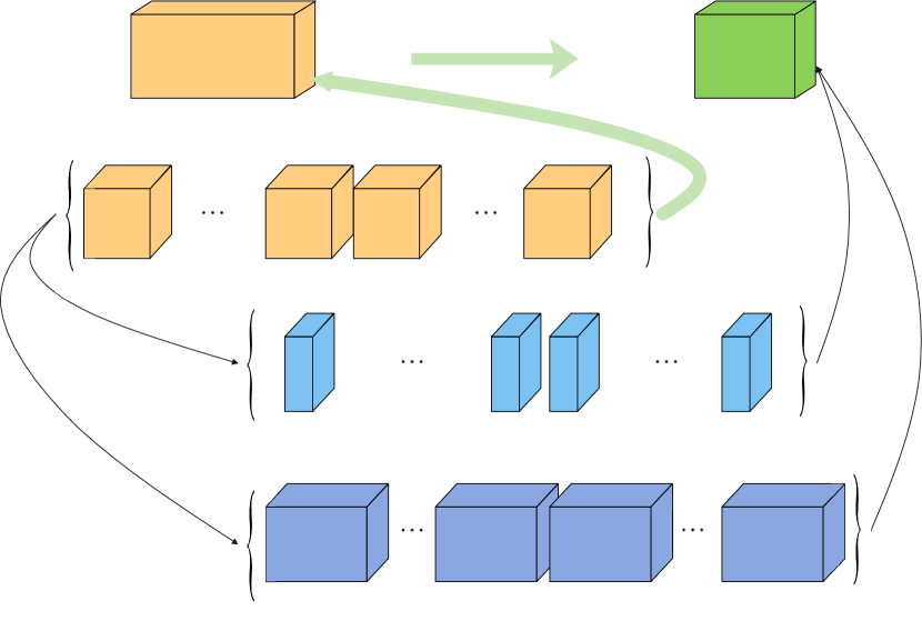
Figure 3: Illustration of how to efficiently construct $\bm{\mathcal{G}}^{\neq n}\times_{2}{\mathcal{S}}$ by sketching the core tensors.

Remark 4.3.

As done in [4], to get the real-valued TR-cores from the real-valued input tensor, we should solve the following equivalent form of Line 12 in Algorithm 4:

$$\bm{\mathcal{G}}_{n}=\mathop{\arg\min}_{\bm{\mathcal{Z}}}\left\|\begin{bmatrix}{\mathfrak{R}}(\hat{{\bf G}}_{S[2]}^{\neq n})\\ {\mathfrak{I}}(\hat{{\bf G}}_{S[2]}^{\neq n})\end{bmatrix}{\bf Z}_{(2)}^{\intercal}-\begin{bmatrix}{\mathfrak{R}}(\hat{{\bf X}}_{S[n]}^{\intercal})\\ {\mathfrak{I}}(\hat{{\bf X}}_{S[n]}^{\intercal})\end{bmatrix}\right\|_{F}.$$

Of course, if the matrices ${\bf F}_{j}$ used in the algorithm are real-valued orthogonal, this process can be ignored. For Algorithm 5, it is very applicable to finding the complex-valued core tensors from the complex-valued input tensor.

4.2 Theoretical analysis

Since the problem we focus on is essentially a sketched least squares problem like the one in [4, 17], we can apply Proposition 2.1 in [17] to our method. The results are given as follows.

Theorem 4.4 (A slight restatement of Proposition 2.1 in [17]).

For the matrices ${\bf G}_{[2]}^{\neq n}$ and ${\bf X}_{[n]}^{\intercal}$ in Eq. 3, denote $rank({\bf G}_{[2]}^{\neq n})=r$ and fix $\varepsilon,\eta\in(0,1)$ such that $\prod_{j\neq n}I_{j}\lesssim 1/\varepsilon^{r}$ with $r\geq 2$. Then a sketching matrix ${\mathcal{S}}\in{\mathbb{C}}^{m\times\prod_{j\neq n}I_{j}}$ used in Algorithms 4 or 5, i.e., Eq. 14 with

$$m=\mathcal{O}\left(\varepsilon^{-1}r^{2(N-1)}\log^{2N-3}(\frac{r}{\varepsilon})\log^{4}(\frac{r}{\varepsilon}\log(\frac{r}{\varepsilon}))\log\prod_{j\neq n}I_{j}\right)$$

is sufficient to output

$$\tilde{{\bf G}}_{n(2)}^{\intercal}=\mathop{\arg\min}_{{\bf G}_{n(2)}^{\intercal}\in{\mathbb{R}}^{R_{n}R_{n+1}\times I_{n}}}\|{\mathcal{S}}{\bf G}_{[2]}^{\neq n}{\bf G}_{n(2)}^{\intercal}-{\mathcal{S}}{\bf X}_{[n]}^{\intercal}\|_{F},$$

such that

$$\mathbf{Pr}\left(\|{\bf G}_{[2]}^{\neq n}\tilde{{\bf G}}_{n(2)}^{\intercal}-{\bf X}_{[n]}^{\intercal}\|_{F}=(1\pm\mathcal{O}\left(\varepsilon\right))\mathop{\min}\|{\bf G}_{[2]}^{\neq n}{\bf G}_{n(2)}^{\intercal}-{\bf X}_{[n]}^{\intercal}\|_{F}\right) \geq 1-\eta-2^{-\Omega(\log\prod_{j\neq n}I_{j})}.$$

Remark 4.5.

It is worth clarifying that the algorithms rTR-ALS,TR-KSRFT-ALS without sampling and TR-CS-ALS listed in Table 1 aren’t covered by the guarantees in the above theorem. This is because there is no step on sampling in these methods.

4.3 Computational complexity

We first analyze the computational complexity of Algorithm 1 because our algorithms are based on TR-ALS. For simplicity, we assume that $I_{n}=I$ and $R_{n}=R$ for all $n\in[N]$ and that $N<I,R^{2}<I$ and $NR<I$. And we ignore any cost associated with e.g. normalization and checking termination conditions.

Upfront costs of TR-ALS:

• Line 2: Initializing cores. This depends on how to initiate the cores. We assume that they are randomly drawn, e.g. from a Gaussian distribution, resulting in a cost $\mathcal{O}\left(NIR^{2}\right)$.

The costs of per outer loop iteration in TR-ALS:

• Line 5: Computing the unfolding subchain tensor. If the $N-1$ cores are dense and contracted in sequence, the cost is

  $$R^{3}(I^{2}+I^{3}+\cdots+I^{N-1})\leq R^{3}(NI^{N-2}+I^{N-1})\leq 2R^{3}I^{N-1}=\mathcal{O}\left(I^{N-1}R^{3}\right).$$

  Doing this for each of the $N$ cores in the inner loop brings the cost to $\mathcal{O}\left(NI^{N-1}R^{3}\right)$.

• Line 6: Solving the least squares problem. We use the standard QR-based approach to analyze the computational complexity. Doing a QR decomposition of ${\bf G}^{\neq n}_{[2]}\in{\mathbb{R}}^{I^{N-1}\times R^{2}}$ costs $\mathcal{O}\left(I^{N-1}R^{4}\right)$, and updating the right hand side and doing back substitution costs $\mathcal{O}\left(I(I^{N-1}R^{2}+R^{4})\right)=\mathcal{O}\left(I^{N}R^{2}\right)$. The leading order complexity for solving the least squares problem is therefore $\mathcal{O}\left(I^{N}R^{2}\right)$. Doing this for each of the N cores in the inner loop brings the cost to $\mathcal{O}\left(NI^{N}R^{2}\right)$.

Putting them all together, we have that the leading order complexity of TR-ALS is

$$\mathcal{O}\left(NIR^{2}+it\cdot NI^{N}R^{2}\right),$$

where “$it$” denotes the number of outer loop iterations.

Now, we present the computational complexity of Algorithm 4.

Upfront costs of TR-KSRFT-ALS:

• Line 2: Initializing cores. It is the same as TR-ALS, which costs $\mathcal{O}\left(NIR^{2}\right)$.

• Line 4: Mixing cores. It costs $\mathcal{O}\left((N-1)I\log I\right)$ because there are $N-1$ cores.

• Line 5: Mixing tensor. It requires a significant upfront cost, which is $\mathcal{O}\left(I^{N}\log(I^{N})\right)$.

The costs of per outer loop iteration in TR-KSRFT-ALS:

• Line 8: Generating $N$ sampling matrices. It costs $\mathcal{O}\left(mN\right)$. Actually, these matrices are not generated explicitly in specific implementation.

• Line 9-Line 10: Computing the sampled subchain tensor. The main cost is the matrix multiplication of $N-1$ matrices of size $R\times R$ for each of the $m$ sampled mode-2 slices, which costs $\mathcal{O}\left(mR^{3}N\right)$ per inner loop iteration, i.e., $\mathcal{O}\left(mR^{3}N^{2}\right)$ per outer loop iteration.

• Line 11: Sampling the input tensor. It needs to copy $\mathcal{O}\left(mI\right)$ elements from the input tensor and then do matrix multiplication. So the cost is $\mathcal{O}\left(mI^{2}\right)$ per inner loop iteration, i.e., $\mathcal{O}\left(NmI^{2}\right)$ per outer loop iteration.

• Line 12: Solving the least squares problem. Similar to TR-ALS, it costs $\mathcal{O}\left(ImR^{2}\right)$ per inner loop iteration, i.e., $\mathcal{O}\left(NImR^{2}\right)$ per outer loop iteration.

• Line 13: Update the mixed cores. It costs $\mathcal{O}\left(I\log I\right)$ per inner loop iteration, i.e., $\mathcal{O}\left(NI\log I\right)$ per outer loop iteration.

It follows that the overall leading order complexity of TR-KSRFT-ALS is

$$\mathcal{O}\left(I^{N}\log(I^{N})+it\cdot NmI^{2}\right),$$

where “$it$” denotes the number of outer loop iterations.

For the computational complexity of TR-KSRFT-ALS-Premix, the analysis is similar. Next we only show the difference:

• Line 15: Unmixing the cores. It costs $\mathcal{O}\left(NI\log I\right)$ because there are $N$ cores.

So the overall leading order complexity of TR-KSRFT-ALS-Premix is

$$\mathcal{O}\left(I^{N}\log(I^{N})+it\cdot NImR^{2}\right),$$

where “$it$” denotes the number of outer loop iterations.

Remark 4.6.

Like Algorithms 4 and 5 in [4], the dominant cost of TR-KSRFT-ALS and TR-KSRFT-ALS-Premix also appears in the upfront costs, i.e., the mixing tensor step. Without considering this cost, i.e., we assume that the data has been preprocessed, the complexities of TR-KSRFT-ALS and TR-KSRFT-ALS-Premix can be reduced remarkably when $I$ and $N$ are huge.

5 TS-based randomized TR decomposition

In this section, we set ${\mathcal{S}}$ to be the TensorSketch ${\bf T}_{\neq n}\in{\mathbb{R}}^{m\times\prod_{j\neq n}I_{j}}$ defined as in Definition 2.11 with $j=1,\ldots,n-1,n+1,\ldots,N$. Thus, from the discussions in Sections 3 and 4, especially Eq. 4 and Proposition 3.6, we can propose the following Algorithm 6 for TR decomposition based on the problem Eq. 3, and the Line 9 is illustrated in Figure 3 and Table 1.

Algorithm 6 TR-TS-ALS (Proposal)

1:function $\{\bm{\mathcal{G}}_{n}\}_{n=1}^{N}$= TR-TS-ALS($\bm{\mathcal{X}},R_{1},\cdots,R_{N},m$) $\triangleright$ $\bm{\mathcal{G}}_{n}\in{\mathbb{R}}^{R_{n}\times I_{n}\times R_{n+1}},n\in[N]$; $\bm{\mathcal{X}}\in{\mathbb{R}}^{I_{1}\times\cdots\times I_{N}}$ $\triangleright$ $R_{1},\cdots,R_{N}$ are the TR-ranks $\triangleright$ $m$ is the embedding size

2:    Define ${\bf S}_{j}$, i.e., the CountSketch, based on $H_{n}$ and $S_{n}$ in Definition 2.11, for $j\in[N]$

3:    for $n=1,\cdots,N$ do

4:        Compute the sketch of ${\bf X}_{[n]}^{\intercal}$: $\hat{{\bf X}}_{[n]}^{\intercal}\leftarrow{\bf T}_{\neq n}{\bf X}_{[n]}^{\intercal}$

5:    end for

6:    Initialize cores $\bm{\mathcal{G}}_{2},\cdots,\bm{\mathcal{G}}_{N}$

7:    repeat

8:        for $n=1,\cdots,N$ do

9:           Compute $\hat{\bm{\mathcal{G}}}^{\neq n}=\operatorname{FFT}^{-1}\left(\boxast_{2~{}j=n+1,\cdots,N}^{~{}~{}1,\cdots,n-1}\operatorname{FFT}\left(\bm{\mathcal{G}}_{j}\times_{2}\mathbf{S}_{j},[~{}],2\right),[~{}],2\right)$

10:           Update $\bm{\mathcal{G}}_{n}=\mathop{\arg\min}_{\bm{\mathcal{Z}}}\|\hat{{\bf G}}_{[2]}^{\neq n}{\bf Z}_{(2)}^{\intercal}-\hat{{\bf X}}_{[n]}^{\intercal}\|_{F}$

11:        end for

12:    until termination criteria met

13:    return $\bm{\mathcal{G}}_{1},\cdots,\bm{\mathcal{G}}_{N}$

14:end function

Remark 5.1.

Algorithm 6 is inspired by the work in [20], which proposes a fast and accurate sketched ALS algorithm for Tucker decomposition by using TensorSketch. Our main contribution is that we find the graceful formula in Proposition 3.6 using the new tensor product and its property. With it, we can design the algorithm as efficiently as in [20].

Similar to Theorem A.7 in [20], we have the following theoretical sketch size for achieving $\mathcal{O}\left(\varepsilon\right)$-relative error.

Theorem 5.2 (A slight restatement of Theorem A.7 in [20]).

For the matrices ${\bf G}_{[2]}^{\neq n}$ and ${\bf X}_{[n]}^{\intercal}$ in Eq. 3, fix $\varepsilon,\eta\in(0,1)$. Then a TensorSketch ${\bf T}_{\neq n}$ used in Algorithm 6 with

$$m=\mathcal{O}\left(((R_{n}R_{n+1}\cdot 3^{N-1})((R_{n}R_{n+1}+1/\varepsilon^{2})/\eta\right),$$

is sufficient to output

$$\tilde{{\bf G}}_{n(2)}^{\intercal}=\mathop{\arg\min}_{{\bf G}_{n(2)}^{\intercal}\in{\mathbb{R}}^{R_{n}R_{n+1}\times I_{n}}}\|{\bf T}_{\neq n}{\bf G}_{[2]}^{\neq n}{\bf G}_{n(2)}^{\intercal}-{\bf T}_{\neq n}{\bf X}_{[n]}^{\intercal}\|_{F},$$

such that

$$\mathbf{Pr}\left(\|{\bf G}_{[2]}^{\neq n}\tilde{{\bf G}}_{n(2)}^{\intercal}-{\bf X}_{[n]}^{\intercal}\|_{F}=(1\pm\mathcal{O}\left(\varepsilon\right))\mathop{\min}\|{\bf G}_{[2]}^{\neq n}{\bf G}_{n(2)}^{\intercal}-{\bf X}_{[n]}^{\intercal}\|_{F}\right)\geq 1-\eta.$$

Now we consider the compliexiy analysis of Algorithm 6. Specifically, with the same assumptions as in Section 4.3, we have the following results.

• Line 2: Generating the $N$ CountSketch matrices. It costs $\mathcal{O}\left(NI\right)$.

• Line 4: Computing the TensorSketch of the input tensor. It costs $\mathcal{O}\left(Nnnz(\bm{\mathcal{X}})\right)$.

• Line 6: Initializing cores. It is the same as TR-ALS, which costs $\mathcal{O}\left(NIR^{2}\right)$.

• Line 9: Computing the TensorSketch of the subchain tensor. It costs

  $$(N-1)nnz(\bm{\mathcal{G}}_{j})+(N-1)mR^{2}\log(m)+(N-2)mR^{3}+mR^{2}\log(m)$$

  $$=\mathcal{O}\left(Nnnz(\bm{\mathcal{G}}_{j})+NmR^{2}\log(m)+NmR^{3}\right)$$

• Line 10: Solving the least squares problem. Similar to TR-ALS, it costs $\mathcal{O}\left(ImR^{2}\right)$ per inner loop iteration, i.e., $\mathcal{O}\left(NImR^{2}\right)$ per outer loop iteration.

As a result, the overall leading order complexity of TR-TS-ALS is

$$\mathcal{O}\left(Nnnz(\bm{\mathcal{X}})+it\cdot NImR^{2}\right),$$

where “$it$” denotes the number of outer loop iterations. So, TR-TS-ALS is very applicable to sparse tensor. For dense tensor, similar to TR-KSRFT-ALS and TR-KSRFT-ALS-Premix, the dominant cost of Algorithm 6 also appears in the upfront costs, i.e., the Line 4.

Remark 5.3.

The leading order computational complexities of the algorithms involved in this paper are summarised in Table 2.

Table 2: Comparison of leading order computational complexities

Method	Complexity	Ignoring mixing tensor
TR-ALS ([35])	$\mathcal{O}\left(NIR^{2}+it\cdot NI^{N}R^{2}\right)$	—–
TR-ALS-Sampled ([25])	$\mathcal{O}\left(NIR^{4}+it\cdot NImR^{2}\right)$	—–
TR-SRFT-ALS (Proposal)	$\mathcal{O}\left(I^{N}\log(I^{N})+it\cdot NmI^{2}\right)$	$\mathcal{O}\left(NIR^{2}+it\cdot NI^{2}m\right)$
TR-SRFT-ALS-Premix (Proposal)	$\mathcal{O}\left(I^{N}\log(I^{N})+it\cdot NImR^{2}\right)$	$\mathcal{O}\left(NIR^{2}+it\cdot NImR^{2}\right)$
TR-TS-ALS (Proposal)	$\mathcal{O}\left(Nnnz(\bm{\mathcal{X}})+it\cdot NImR^{2}\right)$	—–

As before, “$it$” in this table denotes the number of outer loop iterations. From Table 2, we can find that the complexities of TR-SRFT-ALS and TR-SRFT-ALS-Premix are lower than that of the regular TR-ALS, but are higher compared with TR-ALS-Sampled. However, if we don’t consider the complexity of mixing the tensor, our methods will have some advantages over TR-ALS-Sampled. For TR-TS-ALS, its complexity can be lower than that of TR-ALS-Sampled for sparse tensor.

6 Numerical results

To test our proposed methods, we choose two methods as the baselines. The first one is TR-ALS, with which we want to show the advantages of the randomized algorithms for TR decomposition for big data. The second one is TR-ALS-Sampled from [25] because it is the state-of-the-art randomized method for TR decomposition; see the detailed comparison of this method with others given in [25]. Meanwhile, we have also used the same sampling strategy from TR-ALS-Sampled in TR-KSRFT-ALS and TR-KSRFT-ALS-Premix. For TR-ALS and TR-ALS-Sampled, the functions tr_als.m and tr_als_sampled.m from [25] are used in the specific experiments. These two functions are available at https://github.com/OsmanMalik/tr-als-sampled. Additionally, we also use the MATLAB Tensor Toolbox [3].

For the initialization of the involved algorithms, as discussed in [4] on ALS and randomized ALS for CP decomposition, TR-ALS also requires a good starting point to ensure good performance, but the randomized variants gain no obvious advantage from the same initial guess. So, in our experiments, we use random initialization as mentioned in the analysis of computational complexity for randomized algorithms. For TR-ALS, we can choose the results of TR-SVD as the initialization. However, for fairness, we also use random initialization.

In addition, all experiments are run on Matlab R2020b on a computer with an Intel Xeon W-2255 3.7 GHz CPU and 256 GB memory, and all numerical results and plotted quantities are the average over 10 runs.

6.1 Synthetic data

Our experimental method for synthetic tensors can be summarized in the following two stages.

Preparation Stage

In this stage, we use TR-ALS to determine the maximum number of iterations for termination of various algorithms, which will be used as the only termination criterion in Experimental Stage. Specifically, we run TR-ALS until the iterations are larger than $M=500$ or the relative error is smaller than $\varepsilon=1\times 10^{-6}$ and record the iterations $T$. Here, the relative error is defined by

$$\frac{\|\operatorname{TR}\left(\{\bm{\mathcal{G}}^{\prime}_{n}\}_{n=1}^{N}\right)-\bm{\mathcal{X}}\|_{F}}{\|\bm{\mathcal{X}}\|_{F}},$$

where the TR-cores $\bm{\mathcal{G}}^{\prime}_{n}$ are computed by TR-ALS. This relative error is also used to measure the quality of various randomized algorithms for TR decomposition in the subsequent experiments. This is because we have no way to know the true cores in most applications.

Experimental Stage

In this stage, we use $2T$ as the terminationcriterion to run TR-ALS/TR-ALS-Sampled/TR-KSRFT-ALS/TR-TS-ALS. For TR-ALS-Sampled/TR-KSRFT-ALS/TR-TS-ALS, we set the embedding size $m$ to be started at $J_{init}$ and incremented by $J_{inc}$ until $J_{fin}$. In the specific experiments, we set $J_{init}=500$, $J_{inc}=250$, and $J_{fin}=5000$. Thus, we can obtain the corresponding relative errors and running time at each fixed embedding size, and the vectors of relative errors and running time for all the embedding sizes. As for TR-ALS, it doesn’t need the embedding size and its relative error and running time are almost fixed in each experiment. Therefore, with respect to the increase of embedding size, we can plot figures to reflect the variation of relative errors and running time of different algorithms.

Four numerical experiments are carried out to test our methods. All of our synthetic tensors of size $I\times I\times I$ are generated by creating 3 cores of size $R_{true}\times I\times R_{true}$, i.e., $\bm{\mathcal{G}}_{1},\bm{\mathcal{G}}_{2}$ and $\bm{\mathcal{G}}_{3}$, and hence the tensor we are trying to recover is $\bm{\mathcal{X}}_{true}=\operatorname{TR}\left(\{\bm{\mathcal{G}}_{n}\}_{n=1}^{3}\right)$. In the specific experiments, we set $R_{true}=10$ and use $R$ to denote the target rank run in the algorithms. To show the robustness and scalability of algorithms, the noise tensor $\bm{\mathcal{N}}\in{\mathbb{R}}^{I\times I\times I}$ with entries drawn from a standard normal distribution is added into the true tensor. Then the observed tensor is of the following form

$$\bm{\mathcal{X}}=\bm{\mathcal{X}}_{true}+noise\left(\frac{\|\bm{\mathcal{X}}_{true}\|}{\|\bm{\mathcal{N}}\|}\right)\bm{\mathcal{N}},$$

where the parameter $noise$ is the amount of noise. For the sparse tensor, we will only add the noise into the non-zero entries.

In the following, we present the specific way to generate the data and the corresponding numerical results for each of the four experiments.

In the first experiment, we generate a $500\times 500\times 500$ tensor as done in [25]. Specifically, 3 cores of size $10\times 500\times 10$ with entries drawn independently from a standard normal distribution are first created and then one entry for each core is chosen uniformly and set to 20 to increase the coherence. Finally, the true tensor can be formed using TR decomposition.

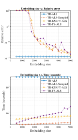
(a) $noise=0$.

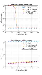
(b) $noise=0.01$.

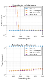
(c) $noise=0.1$.

Figure 4: Embedding sizes v.s. relative errors and running time (seconds) of the first synthetic experiment with true and target ranks $R_{true}=R=10$ and different noises.

Figure 4 shows the numerical results on relative errors and running time for this data with or without noise. From the relative errors shown in the top half of the figure, we can see that TR-KSRFT-ALS and TR-TS-ALS match, and in some cases surpass, the performance of TR-ALS-Sampled, and when the embedding size increases to a certain value, these three methods can achieve similar errors as TR-ALS. For the running time shown in the bottom half of the figure, our two methods and TR-ALS-Sampled have almost the same performance for the case with noise, and are much better than TR-ALS. For the case without noise, our methods perform a little worse than TR-ALS-Sampled, however, still significantly outperform TR-ALS. In addition, when the noise increases, our algorithms are still efficient, which implies that they may be robust to noise.

In the second experiment, we consider the $500\times 500\times 500$ sparse tensor, which is created by 3 cores whose non-zero entries are drawn from a standard normal distribution. Specifically, the 3 cores of size $10\times 500\times 10$ are generated by using the Matlab function sptenrand([10,500,10], density), where $0\leq\texttt{density}\leq 1$ denotes the sparsity. So the core tensor contains approximately $\texttt{density}\times 50000$ normal distributed non-zero entries. In the specific experiments, we set density = 0.05.

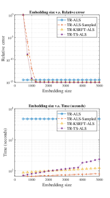
(a) $noise=0$.

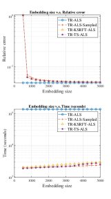
(b) $noise=0.01$.

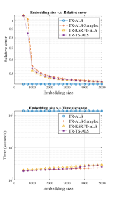
(c) $noise=0.1$.

Figure 5: Embedding sizes v.s. relative errors and running time (seconds) of the second synthetic experiment with true and target ranks $R_{true}=R=10$ and different noises.

Figure 5 shows the numerical results of this experiment. The conclusions from these results are similar to the ones from the first experiment. That is, TR-KSRFT-ALS, TR-TS-ALS and TR-ALS-Sampled have similar performance in relative errors and running time for the data with noise, and if the data has no noise, our methods are a little worse in running time compared with TR-ALS-Sampled. For all the cases, the above three methods always perform much better than TR-ALS in running time. Furthermore, our methods also show superior robustness.

In the third experiment, we use the $500\times 500\times 500$ tensor generated by a method similar to the one in Appendix C.1 of [19] which is used to create data for testing the algorithms for CP decomposition. Specifically, we first create 3 cores of size $10\times 500\times 10$ with entries drawn independently from a standard normal distribution and then set the first three columns of the mode-2 unfolding matrix of each core to be zero. Finally, a few nonzero elements are added to those zero columns. Hence, there are two user-specified parameters in this kind of data: spread and magnitude. $spread$ means how many nonzero elements are added to each column. For example, $spread$ = 15 means that the first 15 rows in the first column, the second 15 rows in the second column, and the third 15 rows in the third column are nonzero. $magnitude$ means the size of the added nonzero elements. In the specific experiments, we set $spread$ = 15, $magnitude=I/4-10$, and do a change on the third core further. That is, we set all the rows except the first 15 ones of the mode-2 unfolding matrix to be zero.

The numerical results for this data are shown in Figure 6. They are a little different from the ones from the previous two experiments. Our algorithms perform better, especially for the case with noise, than TR-ALS-Sampled in terms of the relative errors under almost the same running time. Moreover, to achieve the similar errors as TR-ALS, the embedding sizes of our algorithms are much smaller than that of TR-ALS-sampled. We plot the leverage scores of the classical mode-2 unfolding matrices of the original and transformed TR-cores in Figure 7, which shows that the original cores indeed have some special fibers. This is consistent with the analysis in Remark 4.1.

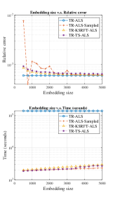
(a) $noise=0$.

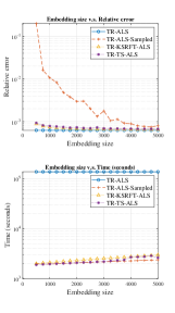
(b) $noise=0.01$.

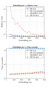
(c) $noise=0.1$.

Figure 6: Embedding sizes v.s. relative errors and running time (seconds) of the third synthetic experiment with true and target ranks $R_{true}=R=10$ and different noises.

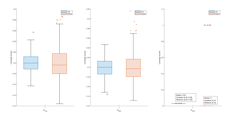
Figure 7: Box plot of leverage scores on the original (right) and transformed (left) TR-cores.

The fourth experiment is mainly used to test Algorithm 5 (TR-KSRFT-ALS-Premix). The complex tensor of size $500\times 500\times 500$ is generated in the same way as the first experiment except that the cores are complex. Figure 8 shows the relative errors and running time for this data with different noises, which is in good agreement with the results shown in the first experiment, and the difference between the running time for data without noise is also not remarkable. So, we can conclude that Algorithm 5 can perform well and is stable under noise for complex data.

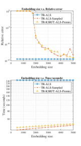
(a) $noise=0$.

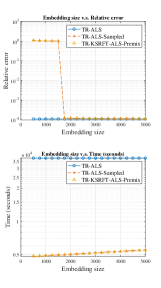
(b) $noise=0.01$.

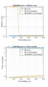
(c) $R=10,noise=0.1$.

Figure 8: Embedding sizes v.s. relative errors and running time (seconds) of the fourth synthetic experiment with true and target ranks $R_{true}=R=10$ and different noises.

6.2 Real data

We consider five real data tensors whose brief information is listed in Table 3 including specific links provided in footnotes.

Table 3: Size and type of real datasets.

Dataset	Size	Type
Indian Pines	$145\times 145\times 220$	Hyperspectral
SalinasA. 4	$83\times 86\times 224$	Hyperspectral
C1-vertebrae	$512\times 512\times 47$	CT Images
Uber.Hour	$183\times 1140\times 1717$	Sparse
Uber.Date 6	$24\times 1140\times 1717$	Sparse

The first two datasets are composed of 3-order tensors containing hyperspectral images, where the first two orders are the image height and width, and the third one is the number of spectral bands. The third dataset consists of $512\times 512\times 47$ tensors where the $512\times 512$ frontal slice of each tensor is a 2-dimensional slice of the C1-vertebrae. These images were obtained from the Laboratory of Human Anatomy and Embryology, University of Brussels (ULB), Belgium. The last two datasets are extracted from the Uber tensor which is a 4-order tensor of size $183\times 24\times 1140\times 1717$ with 3,309,490 nonzeros (0.038%). The entry $(i,j,k,l)$ denotes the number of pickups on date $i$, hour $j$, at latitude $k$ and longitude $l$, in New York city during the period April–August 2014. Due to the limitation of experimental equipment, we divide it into two parts with respect to date and hour respectively, i.e., the Uber.Date and Uber.Hour. The former contains the number of pickups on hour $j$, at latitude $k$ and longitude $l$ for a day, i.e., the entry is $(j,k,l)$, and the latter contains the number of pickups on date $i$, at latitude $k$ and longitude $l$ for an hour, i.e., the entry is $(i,k,l)$.

Considering that the real data always has irregular dimensions, we will not use the same experimental methods as in the second stage in synthetic experiments. Here, we mainly compare the running time and the embedding size $m$ for the same number of iterations and almost the same relative errors. Specifically, we first find the maximum iterations according to the method in the first stage of synthetic experiments with $M=100$ and $\varepsilon=1\times 10^{-3}$. Then, for TR-ALS, we can get the running time and relative error; for other algorithms, we try the embedding size $m$ incrementally using the fixed maximum of iterations until the error is close to the 1.1 times of the TR-ALS error. The size $m$ is started at $J_{init}=2R^{2}$ and incremented by $J_{inc}=100$, and hence $J_{fin}=J_{init}+J_{inc}\times num$, where the target rank $R$ is a priori estimate and is different for different data. Thus, if we record the number of increases for the embedding size, i.e., $num$, we can report the final embedding size $m$. Meanwhile, we can record the running time and the final error for each algorithm. The specific numerical results are presented in Table 4.

Table 4: Decomposition results for real datasets with different target ranks.

Method		TR-ALS	TR-ALS-Sampled	TR-KSRFT-ALS	TR-TS-ALS
Indian Pines ($R=20$)	Error	0.0263	0.0289	0.0289	0.0289
	Time	32.9536	13.7424	12.3571	12.0229
	$num$	-	120	53	73
	Embedding size ($m$)	-	12800	6100	8100
SalinasA. ($R=15$)	Error	0.0066	0.0069	0.0073	0.0073
	Time	4.0225	2.4166	1.8510	2.2868
	$num$	-	54	23	30
	Embedding size ($m$)	-	5850	2750	3450
C1-vertebrae ($R=25$)	Error	0.0804	0.0882	0.0883	0.0883
	Time	409.7951	128.3391	101.7646	156.5089
	$num$	-	228	88	217
	Embedding size ($m$)	-	24050	10050	22950
Uber.Hour ($R=15$)	Error	0.7530	0.8246	0.8272	0.8274
	Time	869.1631	64.7240	39.0307	45.3829
	$num$	-	230	40	47
	Embedding size ($m$)	-	23450	4450	5150
Uber.Date ($R=18$)	Error	0.3864	0.4226	0.4246	0.4239
	Time	1452.1900	159.1936	51.3584	113.8542
	$num$	-	320	46	147
	Embedding size ($m$)	-	32648	5248	15348

Compared with the results of part of the experiments on synthetic data, the performance of our methods on these real data tensors is a little better. Except for TR-TS-ALS on the data C1-vertebrae which still yields substantial speedups over TR-ALS, our methods always outperform TR-ALS-Sampled in running time under almost the same relative errors. This may be mainly because, compared with TR-ALS-Sampled, the embedding sizes of our algorithms are much smaller.

7 Concluding remarks

In this paper, we propose two randomized algorithms, i.e., TR-KSRFT-ALS and TR-TS-ALS, for TR decomposition using KSRFT and TensorSketch. They have pretty decent performance in terms of accuracy and computing time compared with the state-of-the-art method, i.e., TR-ALS-Sampled. To achieve these, two new tensor products are defined and their properties are investigated. These new products and properties are of interest in their own right. For example, they can be used to devise the hybrid algorithms for TR decomposition based on stochastic gradient descent and randomized preconditioning. We will present this work in a subsequent paper. Another future work is to try to reduce the computational cost of the mixing tensor since it usually dominates the total cost of the algorithm.

References

- [1] I. Affleck, T. Kennedy, E. H. Lieb, and H. Tasaki, Valence bond ground states in isotropic quantum antiferromagnets, Comm. Math. Phys., 115 (1988), pp. 477–528, https://doi.org/10.1007/BF01218021.
- [2] S. Ahmadi-Asl, A. Cichocki, A. H. Phan, M. G. Asante-Mensah, M. M. Ghazani, T. Tanaka, and I. V. Oseledets, Randomized algorithms for fast computation of low rank tensor ring model, Mach. Learn.: Sci. Technol., 2 (2020), p. 011001, https://doi.org/10.1088/2632-2153/abad87.
- [3] B. W. Bader, T. G. Kolda, et al., Tensor toolbox for matlab, 2021, https://www.tensortoolbox.org (accessed 2021/04/05). Version 3.2.1.
- [4] C. Battaglino, G. Ballard, and T. G. Kolda, A practical randomized CP tensor decomposition, SIAM J. Matrix Anal. Appl., 39 (2018), pp. 876–901, https://doi.org/10.1137/17M1112303.
- [5] M. Che and Y. Wei, Randomized algorithms for the approximations of Tucker and the tensor train decompositions, Adv. Comput. Math., 45 (2019), pp. 395–428, https://doi.org/10.1007/s10444-018-9622-8.
- [6] M. Che, Y. Wei, and H. Yan, The computation of low multilinear rank approximations of tensors via power scheme and random projection, SIAM J. Matrix Anal. Appl., 41 (2020), pp. 605–636, https://doi.org/10.1137/19M1237016.
- [7] M. Che, Y. Wei, and H. Yan, An efficient randomized algorithm for computing the approximate Tucker decomposition, J. Sci. Comput., 88 (2021), pp. 1–29, https://doi.org/10.1007/s10915-021-01545-5.
- [8] A. Cichocki, N. Lee, I. V. Oseledets, A. H. Phan, Q. Zhao, and D. P. Mandic, Tensor networks for dimensionality reduction and large-scale optimization: Part 1 low-rank tensor decompositions, Found. Trends Mach. Learn., 9 (2016), pp. 249–429, https://doi.org/10.1561/2200000059.
- [9] A. Cichocki, D. Mandic, L. De Lathauwer, G. Zhou, Q. Zhao, C. Caiafa, and H. A. PHAN, Tensor decompositions for signal processing applications: From two-way to multiway component analysis, IEEE Signal Process. Mag., 32 (2015), pp. 145–163, https://doi.org/10.1109/MSP.2013.2297439.
- [10] K. L. Clarkson and D. P. Woodruff, Low-rank approximation and regression in input sparsity time, J. ACM, 63 (2017), pp. 54:1–54:45, https://doi.org/10.1145/3019134.
- [11] H. Diao, Z. Song, W. Sun, and D. P. Woodruff, Sketching for Kronecker product regression and p-splines, in International Conference on Artificial Intelligence and Statistics, vol. 84, Playa Blanca, Lanzarote, Canary Islands, 2018, PMLR, pp. 1299–1308.
- [12] S. V. Dolgov and D. V. Savostyanov, Alternating minimal energy methods for linear systems in higher dimensions, SIAM J. Sci. Comput., 36 (2014), pp. A2248 –A2271, https://doi.org/10.1137/140953289.
- [13] P. Drineas and M. W. Mahoney, Lectures on randomized numerical linear algebra, in The Mathematics of Data, M. W. Mahoney, J. C. Duchi, and A. C. Gilbert, eds., vol. 25 of IAS/Park City Mathematics Series, AMS/IAS/SIAM, 2018, pp. 1–48, https://doi.org/10.1090/pcms/025/00829.
- [14] P. Drineas, M. W. Mahoney, S. Muthukrishnan, and T. Sarlós, Faster least squares approximation, Numer. Math., 117 (2011), pp. 219–249, https://doi.org/10.1007/s00211-010-0331-6.
- [15] T. Gong, Y. Dong, H. Chen, B. Dong, and C. Li, Markov subsampling based huber criterion, 2021, https://arxiv.org/abs/2112.06134.
- [16] T. Gong, Q. Xi, and C. Xu, Robust gradient-based markov subsampling, in Proceedings of the AAAI Conference on Artificial Intelligence, vol. 34(04), New York Hilton Midtown, USA, 2020, AAAI Press, pp. 4004–4011.
- [17] R. Jin, T. G. Kolda, and R. Ward, Faster Johnson-Lindenstrauss transforms via Kronecker products, Inf. Inference, 10 (2021), pp. 1533–1562, https://doi.org/10.1093/imaiai/iaaa028.
- [18] T. G. Kolda and B. W. Bader, Tensor decompositions and applications, SIAM Rev., 51 (2009), pp. 455–500, https://doi.org/10.1137/07070111X.
- [19] B. W. Larsen and T. G. Kolda, Practical leverage-based sampling for low-rank tensor decomposition, 2020, https://arxiv.org/abs/2006.16438.
- [20] L. Ma and E. Solomonik, Fast and accurate randomized algorithms for low-rank tensor decompositions, in Advances in Neural Information Processing Systems, M. Ranzato, A. Beygelzimer, Y. Dauphin, P. Liang, and J. W. Vaughan, eds., vol. 34, Curran Associates, Inc., 2021, pp. 24299–24312.
- [21] O. A. Malik, More efficient sampling for tensor decomposition, 2021, https://arxiv.org/abs/2110.07631.
- [22] O. A. Malik and S. Becker, Low-rank Tucker decomposition of large tensors using TensorSketch, in Advances in Neural Information Processing Systems, vol. 31, Montréal, Canada, 2018, Curran Associates, Inc., pp. 10117–10127.
- [23] O. A. Malik and S. Becker, Fast randomized matrix and tensor interpolative decomposition using CountSketch, Adv. Comput. Math., 46 (2020), https://doi.org/10.1007/s10444-020-09816-9.
- [24] O. A. Malik and S. Becker, Guarantees for the Kronecker fast Johnson-Lindenstrauss transform using a coherence and sampling argument, Linear Algebra Appl., 602 (2020), pp. 120–137, https://doi.org/10.1016/j.laa.2020.05.004.
- [25] O. A. Malik and S. Becker, A sampling-based method for tensor ring decomposition, in Proceedings of the 38th International Conference on Machine Learning, vol. 139, Virtual Event, 2021, PMLR, pp. 7400–7411.
- [26] P.-G. Martinsson and J. A. Tropp, Randomized numerical linear algebra: Foundations and algorithms, Acta Numer., 29 (2020), pp. 403–572, https://doi.org/10.1017/S0962492920000021.
- [27] R. Minster, A. K. Saibaba, and M. E. Kilmer, Randomized algorithms for low-rank tensor decompositions in the Tucker format, SIAM J. Math. Data Sci., 2 (2020), pp. 189–215, https://doi.org/10.1137/19M1261043.
- [28] I. V. Oseledets, Tensor-train decomposition, SIAM J. Sci. Comput., 33 (2011), pp. 2295–2317, https://doi.org/10.1137/090752286.
- [29] R. Pagh, Compressed matrix multiplication, ACM Trans. Comput. Theory, 5 (2013), pp. 1–17, https://doi.org/10.1145/2493252.2493254.
- [30] D. Perez-Garcia, F. Verstraete, M. M. Wolf, and J. I. Cirac, Matrix product state representations, Quantum Inform. Comput., 7 (2007), pp. 401–430.
- [31] N. D. Sidiropoulos, L. De Lathauwer, X. Fu, K. Huang, E. E. Papalexakis, and C. Faloutsos, Tensor decomposition for signal processing and machine learning, IEEE Trans. Signal Process., 65 (2017), pp. 3551–3582, https://doi.org/10.1109/TSP.2017.2690524.
- [32] M. Vandecappelle, Numerical Algorithms for Tensor Decompositions, PhD thesis, Arenberg Doctoral School, Faculty of Engineering Science, 2021.
- [33] D. P. Woodruff, Sketching as a tool for numerical linear algebra, Found. Trends Theor. Comput. Sci., 10 (2014), pp. 1–157, https://doi.org/10.1561/0400000060.
- [34] L. Yuan, C. Li, J. Cao, and Q. Zhao, Randomized tensor ring decomposition and its application to large-scale data reconstruction, in ICASSP 2019 - 2019 IEEE International Conference on Acoustics, Speech and Signal Processing (ICASSP), Brighton Conference Centre Brighton, U.K., 2019, IEEE, pp. 2127–2131.
- [35] Q. Zhao, G. Zhou, S. Xie, L. Zhang, and A. Cichocki, Tensor ring decomposition, 2016, https://arxiv.org/abs/1606.05535.
- [36] G. Zhou, A. Cichocki, and S. Xie, Decomposition of big tensors with low multilinear rank, 2014, https://arxiv.org/abs/1412.1885.