Input Delay Compensation for Neuron Growth by PDE Backstepping

Abstract

Neurological studies show that injured neurons can regain their functionality with therapeutics such as Chondroitinase ABC (ChABC). These therapeutics promote axon elongation by manipulating the injured neuron and its intercellular space to modify tubulin protein concentration. This fundamental protein is the source of axon elongation and its spatial distribution is the state of the axon growth dynamics. Such dynamics often contain time delays because of biological processes. This work introduces an input delay compensation with state-feedback control law for axon elongation by regulating tubulin concentration. Axon growth dynamics with input delay is modelled as coupled parabolic diffusion-reaction-advection Partial Differential Equations (PDE) with a boundary governed by Ordinary Differential Equations (ODE), associated with a transport PDE. A novel feedback law is proposed by using backstepping method for input-delay compensation. The gain kernels are provided after transforming the interconnected PDE-ODE-PDE system to a target system. The stability analysis is presented by applying Lyapunov analysis to the target system in the spatial $\mathcal{H}_{1}$-norm, thereby the local exponential stability of the original error system is proved by using norm equivalence.

1 Introduction

The study about axonal growth is an expanding field in neuroscience in order to understand functionality and structure of neurons (Yamada et al., 1970; Tessier-Lavigne and Goodman, 1996; Kandel et al., 2000). This understanding helps to cure neurological disorders such as spinal cord injury and Alzheimer’s disease (Liu et al., 1997; Maccioni et al., 2001). For example, Chondroitinase ABC is a therapeutic in clinical trials to cure spinal cord injuries. It aims to restore axon growth in damaged neurons by manipulating the extracellular matrix, the non-cellular macromolecules surrounding the cell (Karimi-Abdolrezaee et al., 2010; Bradbury and Carter, 2011; Frantz et al., 2010).

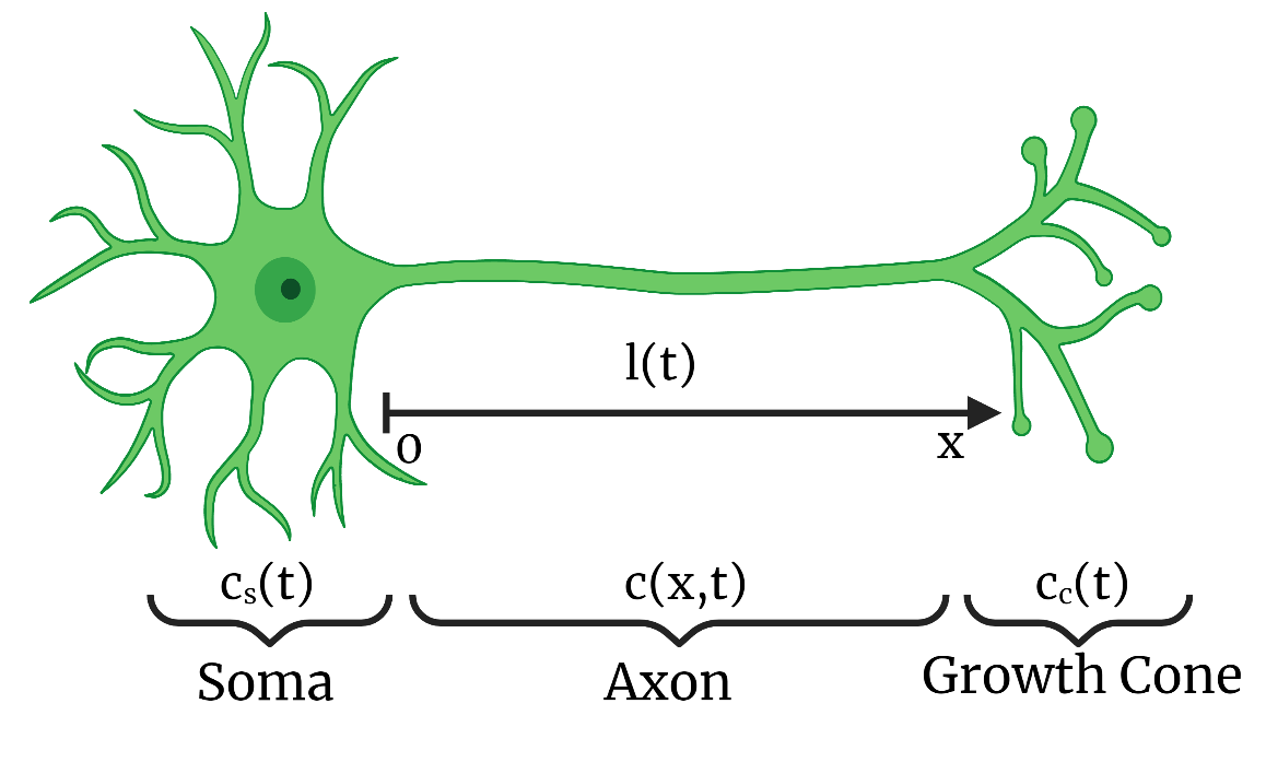
Figure 1: Schematic of neuron and state variables

Neurons are specialized cells in the nervous system that receive and transmit electrical signals. These signals generate perception, and initiate physical actions. Neurons consist of three main components that facilitate perception and give commands to the muscles; the soma, the axon and the growth cone as shown in Fig. 1. The soma is the body of the neuron and is responsible for producing proteins. Dendrites, which resemble tree branches, extend from the soma and receive incoming electrical signals (Kandel et al., 2000). The axon is a wire-like structure that electrical signals travel along. The growth cone is the highly mobile structure at the tip of the axon that seeks chemical cues from the target neuron which will receive the signal. The signal transmission process starts with the entry of an electric signal from the dendrites. The signal then moves along the axon to the growth cone. In the final step, the growth cone identifies the postsynaptic neuron that will receive the signal (Julien, 1999). With the transmission of the signal, the process is complete.

Tubulin proteins play an essential role in signal transmission by serving as the building blocks which extend the axon. Tubulin monomers and dimers build chemical bonds to create microtubules, the tubular protein shape which forms the structure of the axon (Desai and Mitchison, 1997). The creation of microtubules depends on the dynamics of tubulin concentration in the neuron. These dynamics include tubulin production rate, assembly-disassembly rate, and the tubulin transportation process (Diehl et al., 2014). Neurological disorders and external damage, such as spinal cord injuries, can increase the number of axon growth inhibitors that prevent axon elongation (Lemons et al., 1999). In ChABC therapy, bacterial enzymes are injected into damaged tissue to digest axon growth inhibitors which prevent the formation of microtubules (Lee et al., 2010; Frantz et al., 2010). The potential to control microtubule formation motivated researchers to design a control law that manipulates axon elongation to achieve the desired lengths (Demir et al., 2021). Although Demir et al. (2021) provides feedback control law, it does not account for the input time delay between the injected input and the tubulin concentration dynamics. Time delays frequently occur in biological processes and increase the complexity of the system. In this paper, we deal with this problem by applying an input delay compensation with a novel feedback control law.

There are several mathematical models which seek to describe the behavior of tubulin concentration. Van Veen and Van Pelt (1994) presents a nonlinear ODE model which includes the tubulin production at the soma, tubulin transportation, microtubule formation, and axon elongation. Another model expresses the microtubule formation process by linking the mechanics of the membrane and the axon growth (García-Grajales et al., 2017). Besides these ODE models, researchers also developed PDE models that enhance the understanding of the behavior of tubulin concentration and axon elongation (McLean et al., 2004; Diehl et al., 2014). In this model, the authors use a PDE model to describe tubulin concentration along the axon and a nonlinear ODE to describe the axon length. In addition, there is a coupling between PDE and ODE because the length of the axon is the domain of the tubulin concentration in this model. Moreover, McLean and Graham (2006) provides a stability analysis of this coupled PDE-ODE system.

Over the last two decades, the boundary control strategies of PDE-based models have been extensively studied for parabolic, hyperbolic, and some other exotic PDEs (Krstic and Smyshlyaev, 2008). The contribution of Smyshlyaev and Krstic (2004) allowed analytically unsolvable kernel PDEs to be solved numerically by the method of successive approximation, which commenced the usage of boundary control for relatively complex problems. Then, (Susto and Krstic, 2010; Tang and Xie, 2011) extended the boundary control law for the class of coupled PDE and ODE systems. Following this extension, (Krstic, 2009b) introduced input delay compensation for boundary control by considering an input delay as a transport PDE. Krstic (2009a) also provides input delay compensation and control for unstable reaction-diffusion PDE for arbitrarily long input delays. Building on previous studies which examined PDEs with a constant domain size in time, Koga et al. (2018) and Koga and Krstic (2020) developed a backstepping-based boundary control law with global stability results for parabolic PDEs with the moving boundary, called Stefan problem. In addition, delay compensation for the one phase Stefan problem presented in Koga et al. (2020). Buisson-Fenet et al. (2018); Yu et al. (2020) obtained local stability for the class of coupled hyperbolic PDE with a moving boundary governed by an ODE for a piston movement and traffic congestion problems, respectively. In addition, Demir et al. (2021, 2022) provide the local stability results for a parabolic PDE with a moving boundary governed by a nonlinear ODE for the axon growth problem.

This paper presents the feedback stabilization with input delay compensation for the coupled model consisting of tubulin concentration and axon growth. First, we introduce the input delay as a transport PDE. We obtain the reference error system by subtracting the steady-state solution from the dynamics and use linearization to ODE state around the zero state to deal with nonlinearity. Then, we apply backstepping transformations to the transport PDE and the parabolic PDE. While we derive some of the kernels of these transformations analytically, we obtain some of them numerically. By using these kernel solutions, we determine the control law. Finally, we prove the local stability of the original PDE-ODE-PDE system.

This paper is structured as follows. Section II presents the modeling of tubulin concentration and axon growth as a coupled PDE-ODE model with input delay. Section III presents the feedback control law with compensating input delay by using the method of backstepping. The next section proves the stability of the closed-loop system. The paper ends with the conclusion in Section IV.

2 Modeling and Problem Statement

2.1 Axon Growth Model

In this model, tubulin protein is considered as a responsible factor for axon growth with two assumptions. The assumptions are that tubulin is modeled as a homogeneous continuum and that only tubulin is effective for axon growth. Then, axon growth and tubulin concentration with input delay is modeled as

$$c_{t}(x,t)= Dc_{xx}(x,t)-ac_{x}(x,t)-gc(x,t),$$ (1)

$$c_{x}(0,t)= -q_{\rm s}(t-D_{e}),$$ (2)

$$c(l(t),t)= c_{\rm c}(t),$$ (3)

$$l_{\rm c}\dot{c}_{\rm c}(t)= (a-gl_{\rm c})c_{\rm c}(t)-Dc_{x}(l(t),t)$$

$$-(r_{\rm g}c_{\rm c}(t)+\tilde{r}_{\rm g}l_{\rm c})(c_{\rm c}(t)-c_{\infty}),$$ (4)

$$\dot{l}(t)= r_{\rm g}(c_{c}(t)-c_{\infty}),$$ (5)

In (1)-(5), $c(x,t)$ represents tubulin concentration along the axon, $q_{s}$ represents the tubulin flux and subscripts $s$, and $c$ are denoted for soma and growth cone respectively. Namely, $c_{c}(t)$ denotes the tubulin flux in the growth cone, and $q_{s}(t)$ denotes tubulin flux in soma. The axon length is described as $l(t)$ which is in $x$-coordinate. The constants $D$, $a$, and $g$, denote the tubulin diffusion constant, velocity constant, and degradation rate, respectively. $l_{\rm c}$ represents the growth ratio, $r_{\rm g}$ is a lumped parameter, and $\tilde{r}_{\rm g}$ is the microtubule reaction rate. $c_{\infty}$ is the equilibrium of the tubulin concentration in the growth cone. The last constant $D_{e}$ represents the time delay of input.

2.2 Problem Statement

We pursue to drive the axon length to a given desired length $l_{s}>0$ by designing the state feedback control law of $q_{\rm s}(t-D_{e})$ for known time delay, $D_{e}$. The steady-state solution of the system (1)–(5) is then derived by considering an equilibrium of the tubulin concentration $c_{\rm eq}(x)$. Thus, the control objective is to achieve

$$\lim_{t\to\infty}l(t) =l_{\rm s},$$ (6)

$$\lim_{t\to\infty}c(x,t) =c_{eq}(x),$$ (7)

through compensating the input delay $D_{e}$.

2.3 Steady-State Solution

The steady-state solution of the system (1)-(5) is solved for the desired axon length $l_{\rm s}$, which is, as derived in Demir et al. (2021), given by

$$c_{\rm eq}(x)=c_{\infty}\left(K_{+}e^{\lambda_{+}(x-l_{\rm s})}+K_{-}e^{\lambda_{-}(x-l_{\rm s})}\right),$$ (8)

$$q_{\rm s}^{*}=-c_{\infty}\left(K_{+}\lambda_{+}e^{-\lambda_{+}l_{\rm s}}+K_{-}\lambda_{-}e^{-\lambda_{-}l_{\rm s}}\right),$$ (9)

where

$$\lambda_{+}= \frac{a+\sqrt{a^{2}+4Dg}}{2D},\quad\lambda_{-}=\frac{a-\sqrt{a^{2}+4Dg}}{2D},$$ (10)

$$K_{+}= \frac{1}{2}+\frac{a-2gl_{\rm c}}{2\sqrt{a^{2}+4Dg}},\ K_{-}=\frac{1}{2}-\frac{a-2gl_{\rm c}}{2\sqrt{a^{2}+4Dg}}.$$ (11)

2.4 Reference Error System

The reference error states, denoted as $u(x,t)$, $z_{1}(t)$, $z_{2}(t)$ and $U(t-D_{e})$, are defined by

$$u(x,t)= c(x,t)-c_{\rm eq}(x),$$ (12)

$$z_{1}(t)= c_{\rm c}(t)-c_{\infty},$$ (13)

$$z_{2}(t)= l(t)-l_{\rm s},$$ (14)

$$U(t-D_{e})= -(q_{\rm s}(t-D_{e})-q_{\rm s}^{*}).$$ (15)

From (1)-(5), by using (8)-(9), and (12)-(15), we obtain

$$u_{t}(x,t)= Du_{xx}(x,t)-au_{x}(x,t)-gu(x,t),$$ (16)

$$u_{x}(0,t)= U(t-D_{e}),$$ (17)

$$u(l(t),t)= z_{1}(t)+\tilde{h}(z_{2}(t)),$$ (18)

$$\dot{z}_{1}(t)= \tilde{a}z_{1}(t)-\beta u_{x}(l(t),t)-\kappa z_{1}(t)^{2},$$ (19)

$$\dot{z}_{2}(t)= r_{\rm g}z_{1}(t),$$ (20)

where

$$\tilde{a}=\frac{a-r_{\rm g}c_{\infty}}{l_{\rm c}}-g-\tilde{r}_{\rm g},\quad\beta=\frac{D}{l_{\rm c}},\quad\kappa=\frac{r_{\rm g}}{l_{\rm c}},$$ (21)

$$\tilde{h}(z_{2}(t))=c_{\infty}\left(1-K_{+}e^{\lambda_{+}z_{2}(t)}-K_{-}e^{\lambda_{-}z_{2}(t)}\right).$$ (22)

The delayed controller can be represented by the following transport PDE dynamics:

$$v_{t}(x,t)= v_{x}(x,t),\quad D_{e}\geq x\geq 0$$ (23)

$$v(D_{e},t)= U(t).$$ (24)

The solution to this equation is $v(x,t)=U(t+x-D_{e})$ and thus the output $v(0,t)=U(t-D_{e})$ gives the delayed input. Then, let $X\in\mathbb{R}^{2}$ be an ODE state vector for the reference error states $z_{1}(t)$ and $z_{2}(t)$, defined by

$$X(t)=[z_{1}(t)\quad z_{2}(t)]^{\top}.$$ (25)

By using (25), the systematic representation of (16)-(20) and (23)-(24) can be written as

$$u_{t}(x,t)= Du_{xx}(x,t)-au_{x}(x,t)-gu(x,t),$$ (26)

$$u_{x}(0,t)= v(0,t),$$ (27)

$$u(l(t),t)= e_{1}X(t)+\tilde{h}(e_{2}X(t)),$$ (28)

$$\dot{X}(t)= AX(t)+f(X(t))+Bu_{x}(l(t),t),$$ (29)

$$v_{t}(x,t)= v_{x}(x,t),\qquad\qquad D_{e}\geq x\geq 0$$ (30)

$$v(D_{e},t)= U(t).$$ (31)

where

$$A=\left[\begin{array}[]{cc}\tilde{a}&0\\ r_{\rm g}&0\end{array}\right],\ B=\left[\begin{array}[]{c}-\beta\\ 0\end{array}\right],$$ (36)

$$f(X(t))=-\kappa(e_{1}X(t))^{2}e_{1},$$ (37)

where $e_{1}$ and $e_{2}$ are unit vectors; $e_{1}=[1\quad 0]$, $e_{2}=[0\quad 1]$.

2.5 Linearized Reference Error System

Applying linearization around zero states to (26)-(31) leads us to the following linearized system:

$$\dot{X}(t)= AX(t)+Bu_{x}(l(t),t),$$ (38)

$$u_{t}(x,t)= Du_{xx}(x,t)-au_{x}(x,t)-gu(x,t),$$ (39)

$$u(l(t),t)= C^{\top}X(t),$$ (40)

$$u_{x}(0,t)= v(0,t),$$ (41)

$$v_{t}(x,t)= v_{x}(x,t),\quad D_{e}\geq x\geq 0$$ (42)

$$v(D_{e},t)= U(t).$$ (43)

where

$$C=\left[1\quad-\frac{(a-gl_{\rm c})c_{\infty}}{D}\right]^{\top}.$$ (44)

3 State Feedback Design

Before we start introducing the state feedback control law, we use the following notations for several norms:

$$||u(\cdot,t)||_{L_{2}}=\sqrt{\int_{0}^{l(t)}u(.,t)^{2}dx},$$

$$||u(\cdot,t)||_{H_{1}}=\sqrt{\int_{0}^{l(t)}u(.,t)^{2}+u_{x}(.,t)^{2}dx}.$$

In the rest of the paper, we propose the backstepping control law that deals with input delay compensation and stability proof.

3.1 Backstepping Transformation

We consider backstepping transformation of the form

$$w(x,t)= u(x,t)-\int_{x}^{l(t)}k(x,y)u(y,t)dy$$

$$-\phi(x-l(t))X(t),$$ (45)

$$z(x,t)= v(x,t)+\int_{0}^{x}p(x,y)v(y,t)dy$$

$$+\int_{0}^{l(t)}q(x,y)u(y,t)dy+\psi(x-l(t))X(t),$$ (46)

where the kernels $k(x,y)$, $\phi(x)$, $p(x,y)$, $q(x,y)$ and $\psi(x)$ are to be determined to transform the original system to a target system.

$$\dot{X}(t)= (A+BK)X(t)+Bw_{x}(l(t),t)+f(X(t)),$$ (47)

$$w_{t}(x,t)= Dw_{xx}(x,t)-aw_{x}(x,t)-gw(x,t)$$

$$-\dot{l}(t)F(x,X(t))-\phi(x-l(t))^{\top}f(X(t))$$

$$-\left(\phi^{\prime}(x-l(t))^{\top}+\frac{a}{D}\phi(x-l(t))^{\top}\right)B\bar{h}(X),$$ (48)

$$w(l(t),t)= \bar{h}(X(t)),$$ (49)

$$w_{x}(0,t)= z(0,t),$$ (50)

$$z_{t}(x,t)= z_{x}(x,t),$$

$$-\dot{l}(t)\left(q(x,l(t))C^{\top}+\psi^{\prime}(x-l(t))\right)X(t),$$ (51)

$$z(D_{e},t)= 0,$$ (52)

where the nonlinear terms are

$$\tilde{h}(z_{2}(t))= c_{\infty}\left(1-K_{+}e^{\lambda_{+}z_{2}(t)}-K_{-}e^{\lambda_{-}z_{2}(t)}\right),$$ (53)

$$\bar{h}(X)= \left(z_{1}(t)+\tilde{h}(z_{2}(t))\right)-C^{\top}X,$$ (54)

where $K\in\mathbb{R}^{2}$ is a chosen feedback control gain vector to make $A+BK$ Hurwitz. Thus, $K$ is

$$K=[k_{1}\quad k_{2}]^{\top},\quad k_{1}>\frac{\tilde{a}}{\beta},\quad k_{2}>0.$$ (55)

The redundant nonlinear term is

$$F(x,X(t))=\left(\phi^{\prime}(x-l(t))^{T}-k(x,l(t))C^{T}\right)X(t).$$ (56)

3.2 Gain Kernel Solution

The conditions of the kernel functions are obtained to satisfy both the governing equations. Thus, we take the time and spatial derivatives of (45) associated to the solutions of (38)-(41), and then we have the following gain kernel solutions [as detailed in Demir et al. (2021)]

$$\phi(x)^{\top}=\begin{bmatrix}C^{\top}&K^{\top}-\frac{1}{D}C^{\top}BC^{\top}\end{bmatrix}e^{N_{1}x}\begin{bmatrix}I\\ 0\end{bmatrix},$$ (57)

where the matrix $N_{1}\in\mathbb{R}^{4\times 4}$ is defined as

$$N_{1}=\begin{bmatrix}0&\frac{1}{D}\left(gI+A+\frac{a}{D}BC^{\top}\right)\\ I&\frac{1}{D}\left(BC^{\top}+aI\right)\end{bmatrix},$$ (58)

and

$$k(x,y)=\frac{1}{D}\phi(x-y)^{\top}B.$$ (59)

Next, we derive the kernel functions in another transformation (46). Taking time and spatial derivatives of (46) along with (42)-(43), we have the following coupled PDE-ODE for gain kernels

$$q_{x}(x,y)= Dq_{yy}(x,y)+aq_{y}(x,y)-gq(x,y),$$ (60)

$$q(0,y)= -k_{x}(0,y),$$ (61)

$$q(x,l(t))= -\frac{1}{D}\psi(x-l(t))B,$$ (62)

$$q_{y}(x,0)= -\frac{a}{D}q(x,0),$$ (63)

$$\psi^{\prime}(x-l(t))= \psi(x-l(t))A-Dq_{y}(x,l(t))C^{\top}$$

$$-aq(x,l(t))C^{\top},$$ (64)

$$\psi(-l(t))= -\phi^{\prime}(-l(t)).$$ (65)

Through the variable change, and the method of successive approximation, we can show that there exists a unique classic solution for these equations. Then, the last kernel function, $p(x,y)$, is the solution to the following trasport PDE

$$p_{x}(x,y)= -p_{y}(x,y),$$ (66)

$$p(x,0)= -Dq(x,0).$$ (67)

3.3 Inverse Transformation

The inverse transformation of (45)-(46) is formulated as

$$u(x,t) =w(x,t)+\int_{x}^{l(t)}\iota(x,y)w(y,t)dy$$

$$\ \ +\theta(x-l(t))X(t),$$ (68)

$$v(x,t) =z(x,t)-\int_{0}^{x}\varrho(x,y)z(y,t)dy$$

$$\ \ -\int_{0}^{l(t)}\chi(x,y)w(y,t)dy-\varphi(x-l(t))X(t)$$ (69)

Then, by a similar procedure to the derivation in the previous section, we have the kernel functions $\iota(x,y)$, $\theta(x)$, $\varrho(x,y)$, $\chi(x,y)$ and $\varphi(x)$ which are determined as the solution to the following set of PDE-ODE equations:

$$\iota_{xx}(x,y)-\iota_{yy}(x,y)=\frac{a}{D}\left(\iota_{x}(x,y)+\iota_{y}(x,y)\right),$$ (70)

$$\iota_{x}(x,x)+\iota_{y}(y,y)=0,$$ (71)

$$\iota(x,l(t))=-\frac{1}{D}\theta(x-l(t))^{\top}B,$$ (72)

$$D\theta^{{}^{\prime\prime}}(x-l(t))^{\top}+a\theta^{{}^{\prime}}(x-l(t))^{\top}$$

$$\qquad\qquad+\left(gI+A+BK^{\top}\right)\theta(x-l(t))^{\top}=0,$$ (73)

$$\theta(0)=C,\quad\theta^{\prime}(0)=K,$$ (74)

and

$$\chi_{x}(x,y) =-D\chi_{yy}(x,y)-a\chi_{y}(x,y)-g\chi(x,y),$$ (75)

$$\chi_{y}(x,o) =-\frac{a}{D}\chi(x,0),$$ (76)

$$\chi(x,l(t)) =\frac{1}{D}\varphi(x-l(t))^{\top}B,$$ (77)

$$\chi(0,y) =-\iota_{x}(0,y),$$ (78)

$$\varphi^{\prime}(x-l(t))^{\top} =\varphi(x-l(t))^{\top}\left(A+BK^{\top}\right),$$ (79)

$$\varphi(-l(t))^{\top} =\theta^{\prime}(-l(t))^{\top},$$ (80)

$$\varrho_{x}(x,y) =\varrho_{y}(x,y),$$ (81)

$$\varrho(0,t) =-\chi(x,0).$$ (82)

Notice that (70)-(74) are analytically solvable, and the solution of these PDE and ODE equations are detailed in Demir et al. (2021). In addition, (75)-(82) are also analytically solvable, and the solutions are bounded.

3.4 Control Law

Finally, we consider the closed loop system consisting of the plant (47)-(52) and the control law

$$U(t)= -\int_{t-D_{e}}^{t}p(D_{e},\vartheta+D_{e}-t)U(\vartheta)d\vartheta$$

$$-\int_{0}^{l(t)}q(D_{e},y)u(y,t)dy-\psi(D_{e}-l(t))X(t).$$ (83)

(83) is obtained by using the boundary condition (52) in (46), and defining $\vartheta=t+y-D_{e}$ where $\vartheta\in(t-D_{e},t)$ and $v(y,t)=U(t+y-D_{e})$.

4 Stability Analysis

In this section, a local stability of the closed-loop system is presented by considering the $H_{1}$-norm

$$Z(t)=||u(\cdot,t)||_{H_{1}}^{2}+||v(\cdot,t)||_{H_{1}}^{2}+X^{\top}X.$$ (84)

Before presenting our major theorem, we impose the following assumptions.

Assumption 1

The axon length $l(t)$ maintains positive and is upper bounded, i.e., there exists a positive constant $\bar{l}>0$ such that the following inequality holds:

$$0<l(t)\leq\bar{l},$$ (85)

for all $t\geq 0$.

Assumption 2

The time derivative of the axon length is also bounded, i.e., there exists a positive constant $\bar{v}>0$ such that the following inequality holds:

$$\big{|}\dot{l}(t)\big{|}\leq\bar{v},$$ (86)

for all $t\geq 0$.

Assumption 3

The physical constants satisfy the following inequality:

$$\frac{D}{4\bar{l}}\geq a.$$ (87)

Assumption 3 is physically valid and applicable when the axon length is short which is the case for the most of the neurons because average axon length is $20\mu$m-4$0\mu$m (Clark et al., 2009). Then, we state our main result in the following theorem.

Theorem 1

Let Assumption 3 hold. Consider the closed-loop system consisting of the plant (26)–(31) with the control law (83). Then, there exist positive parameters $\bar{K}>0$, $c>0$, and $\kappa>0$, such that if $Z(0)<\bar{K}$ then the following norm estimate holds

$$Z(t)\leq cZ(0)\exp(-\kappa t),$$ (88)

for all $t\geq 0$, which guarantees the local exponential stability of the closed-loop system.

To prove Theorem 1, first we apply the following transformation to (47)-(52)

$$\varpi(x,t)=w(x,t)-xz(0,t)+l(t)z(0,t)-\bar{h}(X),$$ (89)

so we have

$$\dot{X}(t)= (A+BK)X(t)+B\varpi_{x}(l(t),t)+Bz(0,t)$$

$$+f(X(t)),$$ (90)

$$\varpi_{t}(x,t)= D\varpi_{xx}(x,t)-a\varpi_{x}(x,t)-g\varpi(x,t)$$

$$-\bar{h}^{\prime}(X)-g\bar{h}(X)-az(0,t)-gxz(0,t)$$

$$+gl(t)z(0,t)-xz_{t}(0,t)+\dot{l}(t)z(0,t)$$

$$+l(t)z_{t}(0,t)-\dot{l}(t)F(x,X(t))$$

$$-\phi(x-l(t))^{\top}f(X(t))$$

$$-\left(\phi^{\prime}(x-l(t))^{\top}B+\frac{a}{D}\phi(x-l(t))^{\top}B\right)\bar{h}(X),$$ (91)

$$\varpi(l(t),t)= 0,$$ (92)

$$\varpi_{x}(0,t)= 0,$$ (93)

$$z_{t}(x,t)= z_{x}(x,t)$$

$$-\dot{l}(t)\left(\psi^{\prime}(x-l(t))+q(x,l(t))C^{\top}\right)X(t),$$ (94)

$$z(D_{e},t)= 0,$$ (95)

where $x\in(0,l(t))$ for (91)-(93), and $x\in[0,D_{e})$ for (94)-(95).

4.1 Proof of Lyapunov stability

We consider the following Lyapunov function for the target system

$$V=d_{1}V_{1}+V_{2}+d_{2}V_{3}+d_{3}V_{4}+d_{4}V_{5},$$ (96)

where $d_{1}>0$, $d_{2}>0$, $d_{3}>0$ and $d_{4}>0$, and each Lyapunov function is

$$V_{1}:=\frac{1}{2} ||\varpi||_{L_{2}}^{2},\quad V_{2}:=\frac{1}{2}||\varpi_{x}||_{L_{2}}^{2},$$ (97)

$$V_{3}:= \frac{1}{2}\int_{0}^{D_{e}}e^{cx}z^{2}(x,t)dx,$$ (98)

$$V_{4}:= \frac{1}{2}\int_{0}^{D_{e}}e^{cx}z_{x}^{2}(x,t)dx,$$ (99)

$$V_{5}:= X^{\top}PX,$$ (100)

where $c>0$, and $P>0$ is a positive definite matrix satisfying the Lyapunov equation:

$$(A+BK)^{\top}P+P(A+BK)=-Q,$$ (101)

for some positive definite matrix $Q>0$. Since $A+BK^{\top}$ is Hurwitz, due to the positive definiteness of $P$ and $Q$,

$$\lambda_{\rm min}(P)X^{\top}X\leq X^{\top}PX\leq\lambda_{\rm max}(P)X^{\top}X,$$ (102)

holds, where $\lambda_{\max}(P)>\lambda_{\min}(P)>0$ are the largest and smallest eigenvalues in the positive definite matrix $P$. Then, we state the following lemma.

Lemma 1

Let Assumptions 1-2 and 3 are satisfied with

$$\bar{v}=\frac{D-2\epsilon}{8\bar{l}},$$ (103)

where $\epsilon$ can be picked $D>2\epsilon$. Then, for sufficiently large $d_{1}>0$, $d_{2}>0$, $d_{3}>0$ and small $d_{4}>0$, there exist positive constants $\beta_{1}>0$, and $\beta_{2}>0$ such the following norm estimate holds for all $t\geq 0$:

$$\dot{V}\leq-\alpha V+\beta_{1}V^{3/2}+\beta_{2}V^{2},$$ (104)

where

$$\alpha= \min\left\{d_{1}\frac{D}{8},\frac{g}{16},\frac{\lambda_{\rm min}(Q)}{2\lambda_{\min}(P)},c\right\},$$ (105)

$$\beta_{1}= d_{1}\frac{\bar{l}r_{\rm g}}{2}+d_{1}\frac{1}{2}r_{\rm g}+d_{2}e^{cD_{e}}r_{\rm g}+d_{3}e^{cD_{e}}r_{\rm g}+d_{1}\bar{l}r_{\rm g}\frac{L_{4}^{2}}{2}$$

$$+d_{1}r_{\rm g}\frac{L_{2}}{2}+r_{\rm g}\frac{L_{1}}{2}+2d_{4}|P|+d_{2}r_{\rm g}L_{7}+d_{3}r_{\rm g}L_{8},$$ (106)

$$\beta_{2}= d_{1}\frac{r_{\rm g}^{2}}{2}+\frac{1024D_{e}^{2}}{D^{2}}r_{\rm g}^{4}+8D_{e}^{2}\left(1+e^{-cD_{e}}\right)^{2}+\frac{1}{2\varepsilon}L_{5}\kappa$$

$$+d_{1}\frac{1}{\varepsilon}k_{n}L_{6}+\frac{64}{D}r_{\rm g}^{2}\left(\bar{l}^{2}+\frac{\bar{l}^{3}}{3}\right)L_{4}^{2}+\frac{2}{d_{1}D}r_{\rm g}^{2}L_{3}$$

$$+\frac{1}{2\epsilon}L_{5}\kappa+\frac{1}{2\epsilon}k_{n}L_{6}+2h_{n}+8k_{n}^{2}g^{2}.$$ (107)

Taking the time derivative of Lyapunov functions in (97)-(100), using Agmon’s inequality, Poincare’s inequality, Young’s inequality, and Assumptions 1, 2, 3, we obtain

$$\dot{V}\leq -\frac{D}{64}||\varpi_{xx}||^{2}-d_{1}\frac{D}{4}||\varpi_{x}||^{2}-d_{1}\frac{g}{16}||\varpi||^{2}-\frac{d_{2}}{2}|z(0,t)|^{2}$$

$$-\frac{d_{3}}{2}|z_{x}(0,t)|^{2}+d_{1}\frac{|\dot{l}(t)|^{2}}{2}||\varpi(t)||^{2}+\frac{8}{D}|\dot{l}(t)|^{2}|z(0,t)|^{2}$$

$$+d_{1}l(t)\left(\dot{l}(t)G_{1}(l(t))X(t)\int_{0}^{l(t)}\varpi(x,t)dx\right)$$

$$+d_{1}\dot{l}(t)\int_{0}^{l(t)}F(x,X(t))\varpi(x,t)dx$$

$$+\frac{1}{2\varepsilon}\int_{0}^{l(t)}\left(\phi(x-l(t))^{\top}f(X(t))\right)^{2}dx$$

$$+d_{1}\frac{1}{2\varepsilon}\int_{0}^{l(t)}\left(G_{2}(x-l(t))B\bar{h}(X)\right)^{2}dx$$

$$+\dot{l}(t)G_{1}(l(t)))X(t)\int_{0}^{l(t)}\left(l(t)+x\right)\varpi_{xx}(x,t)dx$$

$$+\frac{\big{|}\dot{l}(t)\big{|}}{2}F(l(t),X(t))^{2}$$

$$+\dot{l}(t)\int_{0}^{l(t)}F_{x}(x,X(t))\varpi_{x}(x,t)dx$$

$$+\frac{1}{2\epsilon}\int_{0}^{l(t)}\left(\phi(x-l(t))^{\top}f(X(t))\right)^{2}dx$$

$$+\frac{1}{2\epsilon}\int_{0}^{l(t)}\left(G_{3}(x-l(t))B\bar{h}(X)\right)^{2}dx$$

$$-d_{2}c\int_{0}^{D_{e}}e^{cx}z^{2}(x,t)dx-d_{3}c\int_{0}^{D_{e}}e^{cx}z_{x}^{2}(x,t)dx$$

$$-2d_{2}\dot{l}(t)\int_{0}^{D_{e}}e^{cx}z(x,t)G_{4}(x-l(t))X(t)dx$$

$$-2d_{3}\dot{l}(t)\int_{0}^{D_{e}}e^{cx}z_{x}(x,t)G_{5}(x-l(t))X(t)dx$$

$$-d_{4}\frac{\lambda_{\rm min}(Q)}{2}X^{\top}X+2d_{4}\big{|}P\big{|}\left(X^{\top}X\right)^{3/2}$$

$$+2\bar{h}^{\prime}(X)^{2}+2g^{2}\bar{h}(X)^{2}$$ (108)

where

$$G_{1}(l(t)):=\psi^{\prime}(-l(t))-q(0,l(t))C^{\top},$$ (109)

$$G_{2}(x-l(t)):=-\phi^{\prime}(x-l(t))^{\top}-\frac{1}{D}\phi(x-l(t))^{\top},$$ (110)

$$G_{3}(x-l(t)):=-\phi^{\prime}(x-l(t))^{\top}-\frac{a}{D}\phi(x-l(t))^{\top},$$ (111)

$$G_{4}(x-l(t)):=\psi^{\prime}(x-l(t))-q(x,l(t))C^{\top},$$ (112)

$$G_{5}(x-l(t)):=\psi^{\prime\prime}(x-l(t))-q_{x}(x,l(t))C^{\top},$$ (113)

when we pick

$$d_{1}\geq\frac{4a^{2}}{D^{2}},$$ (114)

$$d_{2}\geq d_{1}\left(g^{2}\frac{\bar{l}^{5}}{6D}+\frac{4(a^{2}+g^{2}\bar{l}^{2})+g}{g}\right)$$

$$\quad\quad+\frac{32(a^{2}+g^{2}\bar{l}^{2})}{D}+\frac{32\bar{l}^{3}}{3D}+d_{4}\frac{4\big{|}B^{T}P\big{|}^{2}}{\lambda_{\rm min}(Q)},$$ (115)

$$d_{3}\geq d_{1}\frac{4\bar{l}^{2}}{g}+d_{1}\frac{4\bar{l}^{3}}{3g}+\frac{32\bar{l}^{5}}{3D}+\frac{32\bar{l}^{3}}{3D},$$ (116)

$$d_{4}\leq\frac{D\lambda_{\rm min}(Q)}{512\bar{l}\big{|}B^{T}P\big{|}^{2}}.$$ (117)

With Assumption 1, there exist positive constants $L_{i}>0$ for $i=1,2,...,5$ such that the following inequalities hold:

$$F(l(t),X(t))^{2}\leq L_{1}X^{\top}X,$$ (118)

$$\int_{0}^{l(t)}F(x,X(t))^{2}dx\leq L_{2}X^{\top}X,$$ (119)

$$\int_{0}^{l(t)}F_{x}(x,X(t))^{2}dx\leq L_{3}X^{\top}X,$$ (120)

$$\left|\psi^{\prime}(-l(t))-q(0,l(t))C^{\top}\right|\leq L_{4},$$ (121)

$$\int_{0}^{l(t)}\phi(x-l(t))^{2}dx\leq L_{5},$$ (122)

$$\int_{0}^{l(t)}\left(G_{2}(x-l(t))B\right)^{2}dx\leq L_{6},$$ (123)

$$\int_{0}^{l(t)}\left(G_{3}(x-l(t))B\right)^{2}dx\leq L_{7}.$$ (124)

In addition, $\dot{l}(t)$ can be rewritten as $\dot{l}(t)=r_{\rm g}e_{1}X$ by (20). For the nonlinear terms, the upper bound for $f(X)$ is derived as

$$f(X(t))\leq\kappa X^{\top}X.$$ (125)

Next, we find the bound for (54). Since the constants defined in (10)-(11) satisfy $\frac{a-gl_{\rm c}}{D}=\lambda_{+}K_{+}+\lambda_{-}K_{-}$, we can show that (54) is equivalent to

$$\bar{h}(X)= c_{\infty}K_{+}(1+\lambda_{+}z_{2}-e^{\lambda_{+}z_{2}})$$

$$+c_{\infty}K_{-}(1+\lambda_{-}z_{2}-e^{\lambda_{-}z_{2}}).$$ (126)

Since we know that $e^{x}\leq 1+x+x^{2}$ for $x<1.79$, we can show the bound of (126) for local region as

$$\left|\bar{h}(X)\right| \leq c_{\infty}(\left|K_{+}\right|(\lambda_{+}z_{2})^{2}+\left|K_{-}\right|(\lambda_{-}z_{2})^{2}).$$ (127)

Now, we can pick $k_{n}=\max\{c_{\infty}K_{+}\lambda_{+}^{2},c_{\infty}K_{-}\lambda_{-}^{2}\}$. Thus,

$$\left|\bar{h}(X)\right| \leq 2\left|k_{n}\right|z_{2}^{2}\leq 2k_{n}X^{\top}X.$$ (128)

Similarly, the upper bound for $\bar{h}^{\prime}(X)$ term is obtained for $x<1.79$ as

$$\bar{h}^{\prime}(X)^{2} \leq h_{n}(X^{\top}X)^{2}$$ (129)

where $h_{n}=\max\left\{2c_{\infty}r_{\rm g}^{2}K_{+}^{2}\lambda_{+}^{4},2c_{\infty}r_{\rm g}^{2}K_{-}^{2}\lambda_{-}^{4}\right\}$.

By using Cauchy-Schwarz, Agmon’s, Young’s inequalities, and the following inequality

$$||z_{x}(x,t)||^{2} \leq\int_{0}^{D_{e}}e^{cx}z_{x}(x,t)^{2}dx\leq e^{cD_{e}}||z_{x}(x,t)^{2}||,$$ (130)

we obtain

$$\dot{V}\leq -d_{1}\frac{D}{8}V_{2}-d_{1}\frac{g}{16}V_{1}-d_{4}\frac{\lambda_{\rm min}(Q)}{2\lambda_{\min}(P)}V_{5}-d_{2}cV_{3}$$

$$-d_{3}cV_{4}+\left(d_{1}\frac{r_{\rm g}\left(\bar{l}+1\right)}{2\lambda_{\min}(P)}+\frac{e^{cD_{e}}r_{\rm g}\left(d_{2}+d_{3}\right)}{\lambda_{\min}(P)}\right)V^{3/2}$$

$$+\left(\frac{d_{1}r_{\rm g}L_{2}}{2\lambda_{\min}(P)}+\frac{r_{\rm g}L_{1}}{2\lambda_{\min}(P)}++\frac{d_{1}\bar{l}r_{\rm g}L_{4}^{2}}{2\lambda_{\min}(P)}\right)V^{3/2}$$

$$+\frac{1}{\lambda_{\min}(P)}\left(2d_{4}|P|+d_{2}r_{\rm g}L_{7}+d_{3}r_{\rm g}L_{8}\right)V^{3/2}$$

$$+\frac{1}{\lambda_{\min}(P)}\left(d_{1}\frac{r_{\rm g}^{2}}{2}+\frac{1024D_{e}^{2}}{D^{2}}r_{\rm g}^{4}+8cD_{e}^{4}+\frac{L_{5}}{2\varepsilon}\kappa\right)V^{2}$$

$$+\frac{1}{\lambda_{\min}(P)}\left(d_{1}\frac{L_{6}+L_{7}}{\varepsilon}k_{n}+\frac{64}{D}r_{\rm g}^{2}\left(\bar{l}^{2}+\frac{\bar{l}^{3}}{3}\right)L_{4}^{2}\right)V^{2}$$

$$+\frac{1}{\lambda_{min}(P)}\left(\frac{2r_{\rm g}^{2}L_{3}}{d_{1}D}+\frac{L_{5}}{2\epsilon}\kappa+\frac{L_{6}}{2\epsilon}k_{n}+2h_{n}\right)V^{2}$$

$$+\frac{1}{\lambda_{\min}(P)}8k_{n}^{2}g^{2}V^{2}.$$ (131)

The inequality above can be written as

$$\dot{V} \leq-\alpha V+\beta_{1}V^{3/2}+\beta_{2}V^{2},$$ (132)

where $\alpha$, $\beta_{1}$ and $\beta_{2}$ are defined in (105)-(107), which completes the proof of Lemma 1.

4.2 Guaranteeing the conditions for all time

Next, we prove the following lemmas to conclude Theorem 1 by ensuring the local stability of the closed-loop system.

Lemma 2

Under Assumption 3, there exists a positive constant $K_{1}>0$ such that in $\Omega_{1}:=\{(\varpi,z,X)\in H_{1}\times H_{1}\times\mathbb{R}^{2}|V(t)<K_{1}\}$, Assumptions 1 and 2 are satisfied.

The definition of $X(t)$ in (25) is equivalent to

$$X(t)=\left[\begin{array}[]{cc}\frac{\dot{l}(t)}{r_{\rm g}}&l(t)-l_{\rm s}\end{array}\right]^{\top}.$$ (134)

Thus, for some $r>0$, if $|X|<r$ then both the following two inequalities hold:

$$\left|\frac{\dot{l}(t)}{r_{\rm g}}\right|<r,\ \ \big{|}l(t)-l_{\rm s}\big{|}<r.$$ (135)

The first inequality ensures that if $r<\frac{\bar{v}}{r_{\rm g}}$ then Assumption 1 holds. The second inequality yields $-r+l_{\rm s}<l(t)<r+l_{\rm s}$, and thus if both $r<l_{\rm s}$ and $r<\bar{l}-l_{\rm s}$ hold, then Assumption 2 holds. Hence, $r>0$ is chosen as

$$r=\min\left\{\frac{\bar{v}}{r_{\rm g}},l_{\rm s},\bar{l}-l_{\rm s}\right\}.$$ (136)

Since the norm of $X$ is bounded as

$$|X|^{2}\leq\frac{1}{\lambda_{\rm min}(P)}X^{\top}PX\leq\frac{d_{4}}{\lambda_{\rm min}(P)}V.$$ (137)

Then, by setting $K_{1}=\frac{\lambda_{\rm min}(P)}{d_{4}}r^{2}$, if $V(t)<K_{1}$ holds then $|X|<r$ and thus Assumptions 1 and 2 are satisfied, by which we can conclude Lemma 2.

Lemma 3

Under Assumption 3, there exists a positive constant $K_{2}>0$ such that if $V(0)<K_{2}$ then the Assumption 1 and 2 are satisfied and the following norm estimate holds:

$$V(t)\leq V(0)e^{-\frac{\alpha}{2}t}.$$ (138)

For a positive constant $K_{2}>0$, let $\Omega:=\{(\varpi,z,X)\in H_{1}\times H_{1}\times\mathbb{R}^{2}|V(t)<K_{2}\}$. If $K_{2}\leq K_{1}$ then $\Omega\subset\Omega_{1}$, and thus the assumptions are satisfied in $\Omega$. Moreover, due to Lemma 1, the norm estimate (104) holds. Hence, by setting

$$K_{2}\leq\frac{-\beta_{2}^{2}\sqrt{\frac{\beta_{1}^{2}(2\alpha\beta_{2}+\beta_{1}^{2})}{\beta_{2}^{4}}}+\alpha\beta_{2}+\beta_{1}^{2}}{2\beta_{2}^{2}},$$ (139)

we can see that applying $V(t)<K_{2}$ to (104) leads to

$$\dot{V}\leq-\frac{\alpha}{2}V,$$ (140)

by which the norm estimate (138) is deduced. Since (138) is a monotonically decreasing function in time, by setting $K_{3}=\min\{K_{1},K_{2}\}$, the region $\Omega$ is shown to be an invariant set. Thus, if $V(0)<K_{3}$, then $V(t)<K_{3}$ for all $t\geq 0$, and one can conclude with Lemma 3. Finally, we show that $(w,z,X)$ system is locally exponentially stable. Taking the square of (89) and applying Young’s and Cauchy-Schwarz inequalities, we obtain

$$||\varpi(\cdot,t)||_{H_{1}}^{2}\leq 3||w(\cdot,t)||_{H_{1}}^{2}+M_{1}||z(\cdot,t)||_{H_{1}}^{2}+M_{2}|X|^{2},$$ (141)

$$||w(\cdot,t)||_{H_{1}}^{2}\leq 3||\varpi(\cdot,t)||_{H_{1}}^{2}+M_{1}||z(\cdot,t)||_{H_{1}}^{2}+M_{2}|X|^{2},$$ (142)

where $M_{1}=4D_{e}^{3}\bar{l}+4D_{e}\bar{l}^{3}$ and $M_{2}=12k_{n}^{2}$. Consider the norm $\Pi(x,t)=||w(x,t)||_{H_{1}}^{2}+||z(x,t)||_{H_{1}}^{2}+|X(t)|^{2}$. By using (130), we can show that

$$||z(.,t)||_{H_{1}}^{2}\leq V_{3}+V_{4}\leq e^{cD_{e}}||z(.,t)||_{H_{1}}^{2},$$ (143)

and

$$M_{3}||w(.,t)||_{H_{1}}^{2}\leq 2V_{1}+2V_{2}\leq M_{4}||w(.,t)||_{H_{1}}^{2},$$ (144)

where $M_{3}=\max\{\bar{l}^{2},1\}$ and $M_{4}=\max\{\frac{1}{\bar{l}^{2}},1\}$. Then, we have

$$\Pi(t)\leq \left(1+M_{1}\right)||z_{x}(x,t)|||_{H_{1}}^{2}+3||\varpi(x,t)||_{H_{1}}^{2}$$

$$+(1+M_{2})|X(t)|^{2}$$

$$\leq (2+2M_{1})(V_{3}+V_{4})+12(V_{1}+V_{2})+\frac{1+M_{2}}{\lambda_{\min}(P)}V_{5}$$ (145)

By using (96), we have

$$V\leq \left(\max\{d_{2},d_{3}\}e^{cD_{e}}+\frac{M_{1}M_{3}}{2}\max\{d_{1},1\}\right)||z(.,t)||_{H_{1}}^{2}$$

$$+\frac{3M_{3}}{2}\max\{d_{1},1\}||w(.,t)||_{H_{1}}^{2}$$

$$+\left(\frac{d_{4}}{\lambda_{\min}(P)}+\frac{M_{2}M_{3}}{2}\max\{d_{1},1\}\right)|X(t)|^{2}$$

$$\leq \Sigma_{1}||z(.,t)||_{H_{1}}^{2}+\Sigma_{2}||w(.,t)||_{H_{1}}^{2}+\Sigma_{3}|X(t)|^{2}$$ (146)

where $\Sigma_{1}=\max\{d_{2},d_{3}\}e^{cD_{e}}+\frac{M_{1}M_{3}}{2}\max\{d_{1},1\}$, $\Sigma_{2}=\frac{3M_{3}}{2}\max\{d_{1},1\}$ and $\Sigma_{3}=\frac{d_{4}}{\lambda_{\min}(P)}+\frac{M_{2}M_{3}}{2}\max\{d_{1},1\}$. Therefore, (145) and (146) leads us the following norm equivalence

$$\underline{$\delta$}V(t)\leq\Pi(t)\leq\bar{\delta}V(t)$$ (147)

where

$$\underline{$\delta$} =\frac{1}{\max\left\{\Sigma_{1},\Sigma_{2},\Sigma_{3}\right\}},$$ (148)

$$\bar{\delta} =\max\left\{(2+2M_{1}),12,\frac{1+M_{2}}{\lambda_{\min}(P)}\right\}.$$ (149)

With the inequalities (138) and (147), we show that

$$\Pi(t)\leq\frac{\bar{\delta}}{\underline{$\delta$}}\Pi(0)e^{-\frac{\alpha}{2}},$$ (150)

which ensures the exponential stability of $(w,z,X)$-system. Finally, owing to Lemma 3 and (150), and using the similar norm equivalent estimate in the $H_{1}$-norm between the target system $(w,z,X)$ and the closed-loop system $(u,v,X)$, the local stability of the closed-loop system is proved, which completes the proof of Theorem 1.

5 Conclusion

This paper proposes a novel feedback control law with input delay compensation for a PDE with a moving boundary governed by an ODE. The input delay is represented by a transport PDE dynamics, and the controller is designed by PDE backstepping for stabilizing the PDE-ODE system with compensating the input delay. For further research, the observer design can be studied under delayed outputs so that the unknown state variables can be estimated through compensating the delayed measured output.

References

• Bradbury and Carter (2011) Bradbury, E.J. and Carter, L.M. (2011). Manipulating the glial scar: chondroitinase abc as a therapy for spinal cord injury. Brain research bulletin, 84(4-5), 306–316.
• Buisson-Fenet et al. (2018) Buisson-Fenet, M., Koga, S., and Krstic, M. (2018). Control of piston position in inviscid gas by bilateral boundary actuation. In 2018 IEEE Conference on Decision and Control (CDC), 5622–5627. IEEE.
• Clark et al. (2009) Clark, B.D., Goldberg, E.M., and Rudy, B. (2009). Electrogenic tuning of the axon initial segment. The Neuroscientist, 15(6), 651–668.
• Demir et al. (2021) Demir, C., Koga, S., and Krstic, M. (2021). Neuron growth control by pde backstepping: Axon length regulation by tubulin flux actuation in soma. In 2021 60th IEEE Conference on Decision and Control (CDC), 649–654. 10.1109/CDC45484.2021.9683188.
• Demir et al. (2022) Demir, C., Koga, S., and Krstic, M. (2022). Neuron growth output-feedback control by pde backstepping. arXiv preprint arXiv:2203.16733.
• Desai and Mitchison (1997) Desai, A. and Mitchison, T.J. (1997). Microtubule polymerization dynamics. Annual review of cell and developmental biology, 13(1), 83–117.
• Diehl et al. (2014) Diehl, S., Henningsson, E., Heyden, A., and Perna, S. (2014). A one-dimensional moving-boundary model for tubulin-driven axonal growth. Journal of theoretical biology, 358, 194–207.
• Frantz et al. (2010) Frantz, C., Stewart, K.M., and Weaver, V.M. (2010). The extracellular matrix at a glance. Journal of cell science, 123(24), 4195–4200.
• García-Grajales et al. (2017) García-Grajales, J.A., Jérusalem, A., and Goriely, A. (2017). Continuum mechanical modeling of axonal growth. Computer Methods in Applied Mechanics and Engineering, 314, 147–163.
• Julien (1999) Julien, J.P. (1999). Neurofilament functions in health and disease. Current opinion in neurobiology, 9(5), 554–560.
• Kandel et al. (2000) Kandel, E.R., Schwartz, J.H., Jessell, T.M., Siegelbaum, S., Hudspeth, A.J., and Mack, S. (2000). Principles of neural science, volume 4. McGraw-hill New York.
• Karimi-Abdolrezaee et al. (2010) Karimi-Abdolrezaee, S., Eftekharpour, E., Wang, J., Schut, D., and Fehlings, M.G. (2010). Synergistic effects of transplanted adult neural stem/progenitor cells, chondroitinase, and growth factors promote functional repair and plasticity of the chronically injured spinal cord. Journal of Neuroscience, 30(5), 1657–1676.
• Koga et al. (2020) Koga, S., Bresch-Pietri, D., and Krstic, M. (2020). Delay compensated control of the stefan problem and robustness to delay mismatch. International Journal of Robust and Nonlinear Control, 30(6), 2304–2334.
• Koga et al. (2018) Koga, S., Diagne, M., and Krstic, M. (2018). Control and state estimation of the one-phase stefan problem via backstepping design. IEEE Transactions on Automatic Control, 64(2), 510–525.
• Koga and Krstic (2020) Koga, S. and Krstic, M. (2020). Materials Phase Change PDE Control and Estimation: From Additive Manufacturing to Polar Ice. Springer Nature.
• Krstic (2009a) Krstic, M. (2009a). Control of an unstable reaction–diffusion pde with long input delay. Systems & Control Letters, 58(10-11), 773–782.
• Krstic (2009b) Krstic, M. (2009b). Delay compensation for nonlinear, adaptive, and pde systems.
• Krstic and Smyshlyaev (2008) Krstic, M. and Smyshlyaev, A. (2008). Boundary control of PDEs: A course on backstepping designs. SIAM.
• Lee et al. (2010) Lee, H., McKeon, R.J., and Bellamkonda, R.V. (2010). Sustained delivery of thermostabilized chabc enhances axonal sprouting and functional recovery after spinal cord injury. Proceedings of the National Academy of Sciences, 107(8), 3340–3345.
• Lemons et al. (1999) Lemons, M.L., Howland, D.R., and Anderson, D.K. (1999). Chondroitin sulfate proteoglycan immunoreactivity increases following spinal cord injury and transplantation. Experimental neurology, 160(1), 51–65.
• Liu et al. (1997) Liu, X.Z., Xu, X.M., Hu, R., Du, C., Zhang, S.X., McDonald, J.W., Dong, H.X., Wu, Y.J., Fan, G.S., Jacquin, M.F., et al. (1997). Neuronal and glial apoptosis after traumatic spinal cord injury. Journal of Neuroscience, 17(14), 5395–5406.
• Maccioni et al. (2001) Maccioni, R.B., Muñoz, J.P., and Barbeito, L. (2001). The molecular bases of alzheimer’s disease and other neurodegenerative disorders. Archives of medical research, 32(5), 367–381.
• McLean and Graham (2006) McLean, D.R. and Graham, B.P. (2006). Stability in a mathematical model of neurite elongation. Mathematical medicine and biology: a journal of the IMA, 23(2), 101–117.
• McLean et al. (2004) McLean, D.R., van Ooyen, A., and Graham, B.P. (2004). Continuum model for tubulin-driven neurite elongation. Neurocomputing, 58, 511–516.
• Smyshlyaev and Krstic (2004) Smyshlyaev, A. and Krstic, M. (2004). Closed-form boundary state feedbacks for a class of 1-d partial integro-differential equations. IEEE Transactions on Automatic Control, 49(12), 2185–2202.
• Susto and Krstic (2010) Susto, G.A. and Krstic, M. (2010). Control of pde–ode cascades with neumann interconnections. Journal of the Franklin Institute, 347(1), 284–314.
• Tang and Xie (2011) Tang, S. and Xie, C. (2011). State and output feedback boundary control for a coupled pde–ode system. Systems & Control Letters, 60(8), 540–545.
• Tessier-Lavigne and Goodman (1996) Tessier-Lavigne, M. and Goodman, C.S. (1996). The molecular biology of axon guidance. Science, 274(5290), 1123–1133.
• Van Veen and Van Pelt (1994) Van Veen, M.P. and Van Pelt, J. (1994). Neuritic growth rate described by modeling microtubule dynamics. Bulletin of mathematical biology, 56(2), 249–273.
• Yamada et al. (1970) Yamada, K.M., Spooner, B.S., and Wessells, N.K. (1970). Axon growth: roles of microfilaments and microtubules. Proceedings of the National Academy of Sciences, 66(4), 1206–1212.
• Yu et al. (2020) Yu, H., Diagne, M., Zhang, L., and Krstic, M. (2020). Bilateral boundary control of moving shockwave in lwr model of congested traffic. IEEE Transactions on Automatic Control.