Reliability and robustness of oscillations in some slow-fast chaotic systems

Abstract

A variety of nonlinear models of biological systems generate complex chaotic behaviors that contrast with biological homeostasis, the observation that many biological systems prove remarkably robust in the face of changing external or internal conditions. Motivated by the subtle dynamics of cell activity in a crustacean central pattern generator (CPG), this paper proposes a refinement of the notion of chaos that reconciles homeostasis and chaos in systems with multiple timescales. We show that systems displaying relaxation cycles while going through chaotic attractors generate chaotic dynamics that are regular at macroscopic timescales and are thus consistent with physiological function. We further show that this relative regularity may break down through global bifurcations of chaotic attractors such as crises, beyond which the system may also generate erratic activity at slow timescales. We analyze these phenomena in detail in the chaotic Rulkov map, a classical neuron model known to exhibit a variety of chaotic spike patterns. This leads us to propose that the passage of slow relaxation cycles through a chaotic attractor crisis is a robust, general mechanism for the transition between such dynamics. We validate this numerically in three other models: a simple model of the crustacean CPG neural network, a discrete cubic map, and a continuous flow.

Some biological models are known to exhibit mathematical chaos, yet are considered by biologists to have regular dynamics capable of maintaining biological function. These systems typically display highly erratic behaviors at short timescales but maintain regular features at slower, physiologically relevant timescales. We explore this conundrum mathematically and identify mathematical structures which allow chaotic deterministic systems with multiple timescales to maintain macroscopic regularity. We also exhibit a general global bifurcation mechanism that can cause these systems to transition to highly erratic behaviors at slow timescales.

I Introduction

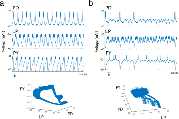
Figure 1: Intracellular voltage traces from 3 pyloric circuit neurons of the Cancer borealis STG. (a) Chaotic behaviors in an intact system showing rhythmic bursting with low fluctuations in the period of oscillations (with a coefficient of variation $c_{v}=0.02$), and (b) Erratic bursting/firing dynamics in a decentralized network, where the irregularity in the slow dynamics is characterized by sizable fluctuations of the relaxation cycle duration ($c_{v}=0.63$).

Deterministic dynamical systems that feature chaotic dynamics are usually characterized by irregular aperiodic patterns of activity and unpredictable behaviors which are highly sensitive to perturbations of parameters and initial conditions. These erratic characteristics of chaotic dynamical systems seem to be undesirable for physiological biological systems that are required to maintain robust activity patterns to function. However, the presence of chaotic dynamics has been reported in several experiments on physiological behavior, including key functions such as cardiac contractions Hayashi and Ishizuka (1992) or brain activity Korn and Faure (2003), and many of these systems demonstrate highly regular dynamics at physiological timescales, with irregular activity limited to small timescales and rapid fluctuations. A well-studied biological system exhibiting such behaviors is the stomatogastric ganglion (STG) of crustaceans Kedia and Marder (2022) described below. In this paper, we explore how deterministic dynamical systems can exhibit this interplay between fast chaos and slow periodicity.

Beyond its conceptual interest, the interplay between irregular activity and biological function has implications in understanding possible consistency between chaos and homeostasis, the process by which a variety of functions of living organisms are regulated in response to changes in the environment Bernard (1879); May et al. (1998); Dijk et al. (1999); Aronoff et al. (2004). Various system-level feedback control mechanisms have been suggested to maintain macroscopic activity (see e.g., in neuroscience,  Turrigiano and Nelson (2004); Cannon and Miller (2016); Marder and Tang (2010); Naudé et al. (2013)). At the single-cell level and in the absence of an exogenous mechanism, homeostasis has been suggested to be devoid of chaos Goldberger (1991). It was associated with the existence of stable fixed points that show little dependence to parameters Reed et al. (2017); Golubitsky and Stewart (2018); Golubitsky and Wang (2020) or robust limit cycles Yu and Thomas (2022). However, an example of a chaotic system showing considerable robustness is given by the crustacean STG, a motor neural circuit producing a stable triphasic bursting pattern of activity that controls the movements of muscles involved in chewing and filtering food (see review Marder and Bucher (2007)). This neural network is remarkably robust to changes in internal and external conditions (Fig. 1a) and is able to maintain constant key features for functional output such as the order of firing of the neural populations, relative phases, and duty cycles. These macroscopic regularities arise despite a clear cycle-to-cycle variability typical of chaotic systems (covering a dense region of the phase space, Fig. 1a, bottom) which is also reflected in various detailed models of the system Alonso and Marder (2020, 2019). However, this chaos can significantly impact function when the neurohormonal inputs to the STG are blocked (a process called decentralization), yielding an erratic spiking behavior with sporadic bursts and a complete loss of rhythmicity, associated with a loss of function (Fig. 1b). In this work, we consider the question of whether purely deterministic systems can display these two types of chaotic behavior and how such systems can switch between them. While we only briefly address stochastic slow-fast systems, the results of this paper are also relevant in this context as well, cf. Fig. 10.

From the mathematical viewpoint, all formal definitions of chaos to date rely on fine properties of the dynamical system Sander and Yorke (2015), and in particular possible regularities arising at slower timescales are immaterial in these characterizations. The main contribution of this paper is to refine the notions of chaos in the context of deterministic dynamical systems with multiple timescales so as to to distinguish whether or not chaos affects the macroscopic behavior of the system at slow timescales.

This paper proceeds as follows. We start by proposing a definition of slow and fast chaos in section II, before proceeding to a detailed analysis of the chaotic Rulkov map in section III with a particular focus on exhibiting these types of dynamics and the transitions between them. Section IV proposes a topological account for the dynamics observed in these two regimes that we validate using a probabilistic model for characterizing the slow-fast behavior of the chaotic Rulkov map. We then explore the generality of these findings by studying a variety of models. We first return to the CPG motivation in section V and introduce a simple network model with behavior similar to the CPG network in Fig. 1. Section VI goes further into exploring the generality of the behaviors described and introduces two other models which contain slow and fast chaos. Source codes for all numerical simulations are available at Jaquette et al. (2023) and the numerical methods used in these simulations are discussed in the Appendix.

II Slow and Fast Chaos

There are several definitions of chaos reflecting the variety of facets of the phenomenon Sander and Yorke (2015). The most classical characterizations of chaos involve positive Lyapunov exponents, topological entropy, or information entropy. In our context, a natural question is whether any of these characterizations is able to distinguish between chaos on the slow and the fast timescales, since from the point of view of applications, these are qualitatively quite different.

Central to our definition of fast or slow chaos, we will focus our attention on the timing of specific events arising at the slow timescale. If, for a system displaying chaos, the fluctuations in the timing of these events are negligible compared to the slow timescale, we will qualify this chaotic behavior as fast chaos. Instead, if the fluctuations are of the same order of magnitude as the slow timescale, we will qualify the behavior as slow chaos.

To make this qualitative definition more quantitative, we propose the following empirical description. We consider a sequence of events arising at the slow timescale For example, in data this time scale could be characterized by events such as directional threshold crossings, switches between biologically relevant regimes such as the up- and down-states in Fig. 1, or Poincaré sections. The duration of the time interval separating such events defines a sequence of real numbers $(\tau_{n})_{n\geq 0}$, with a mean $\bar{\tau}$ and standard deviation $\Sigma$. The so-called coefficient of variation is defined as $c_{v}:=\bar{\tau}/\Sigma$. A coefficient of variation $c_{v}$ of order $1$ characterizes trajectories where the fluctuations in the timings of the slow events are of the same order of magnitude as their means, which is characteristic of orbits $O_{N}$ that are slowly chaotic. If instead $c_{v}$ is small compared to $1$, then the fluctuations in these timings are small compared to the mean, corresponding to trajectories that are regular at slow timescales and thus displaying fast chaos in this parlance. Another relevant dimensionless quantity that we will consider is the level of fluctuations in the timing of the slow events (measured using the standard deviation of return times) relative to the slow timescale, $\tilde{\Sigma}=\Sigma\cdot\mu$ where $\mu$ is the inverse characteristic time of the slow variables. If $\tilde{\Sigma}$ is of order one, the fluctuations in the timing of slow events are on the same order of magnitude as the slow timescale, corresponding heuristically to slow chaos. Instead, if $\tilde{\Sigma}$ is small compared to $1$, the events arise at regular intervals compared to the slow timescale and we have fast chaos.

Maslennikov and Nekorkin Maslennikov and Nekorkin (2016) reported, for the first time to our knowledge, the possibility of the emergence of chaotic trajectories with relatively regular slow trajectories in idealized mathematical models and discrete FitzHugh-Nagumo maps. Such trajectories are akin to what we classify as fast chaos in this paper. In the same vein, chaotic trajectories with regular slow dynamics were reported in periodically forced cubic maps Han et al. (2017). In these systems, the regularity of the slow dynamics is imposed by a slow periodic variation of a parameter in the equation, while chaos emerges at a much faster timescale due to the instabilities of the fast dynamics. Another highly relevant work is the analysis of Terman Terman (1992) of chaotic trajectories in slow-fast systems of differential equations describing neural systems with relaxation cycles in the vicinity of a bifurcation from periodic bursting behavior to spiking behavior. This takes place in the vicinity of homoclinic orbits, and may arise in three-dimensional differential equations which do not include the possibility of fast chaos.

III The Chaotic Rulkov Map

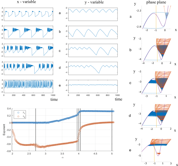
Figure 2: Top: Chaotic trajectories of the Rulkov map, at parameters $\mu=0.01,\sigma=-1$ with subfigures $a,b,c,d,e$ corresponding resp. to $\alpha=2.698$, $3.95$, $4.00$, $4.05$, $5.00$. Left: $x_{n}$; Middle: $y_{n}$; Right: Phase planes for $x$ versus $y$ showing an orbit for $\mu=0.01$ (blue), the fast attractor for $\mu=0$ (red), the fast nullcline (purple), and the slow nullcline (yellow). Bottom Left: Lyapunov exponents as a function of $\alpha$, indicating that chaos emerges when $\alpha\approx 2.6$.

The core of this paper relies on the analysis of the chaotic Rulkov map introduced in Rulkov (2001). This model was shown to encompass, within a simple two-dimensional discrete dynamical system preserving mathematical tractability, some of the most prominent neuronal behaviors Ibarz et al. (2011); Courbage and Nekorkin (2010). This map is given by:

$$x_{n+1} =\frac{\alpha}{1+x_{n}^{2}}+y_{n}$$ (1)

$$y_{n+1} =y_{n}-\mu\;(x_{n}-\sigma).$$ (2)

The dimensionless variable $x_{n}$ models the membrane potential of a neuron at discrete time step $n$, and $y_{n}$ is an adaptation variable accounting for slower gating processes. The resting potential is denoted by $\sigma$, which will be fixed to $\sigma=-1$ for the rest of the study. The small parameter $\mu$ denotes the timescale ratio of adaptation compared to voltage, and the parameter $\alpha$ controls the excitability of the neuron. This excitability parameter $\alpha$ will serve as our main bifurcation parameter in this study. As the neuron becomes more excitable, it transitions from a resting state to an invariant cycle  which rapidly grows into a large amplitude relaxation cycle that eventually becomes chaotic upon increasing excitability, as shown in Fig. 2 (see also (Ibarz et al., 2011, Section 2.1.2)). A fine analysis of these chaotic trajectories identifies distinct classes of behaviors, as we depict in Fig. 2:

• For $\alpha$ just above the value associated with the emergence of a positive Lyapunov exponent, we observe marginally chaotic orbits with regular relaxation cycles exhibiting fluctuating patterns on the crest of the relaxation cycle.

• As $\alpha$ is further increased, we continue to observe relatively regular relaxation cycles, yet bursts become more complex and show higher amplitude spikes with a repetitive triangular profile, which is notwithstanding all distinct and non-periodic.

• Beyond a threshold level for $\alpha$, the slow dynamics suddenly becomes irregular, with long bursts with triangular spike profiles (as described in (b)) alternating non-periodically with shorter bursts with approximately constant spike amplitude (yielding rectangular-shaped envelopes).

• As $\alpha$ is further increased, slow chaos persists, with shorter bursts becoming more frequent and longer bursts rarer.

• Eventually, the system reaches a threshold value of $\alpha$ beyond which the system no more produces relaxation cycles and the orbit is continuously bursting/spiking, with no discernable separation of bursts.

As expected, the study of Lyapunov exponents precisely identifies the presence of chaos. However, these exponents do not appear to identify a transition between fast chaos (with relatively regular repetitions of chaotic bursts) and slow chaos with irregular alternations of longer triangular bursts and briefer square bursts. A close inspection of the second Lyapunov exponent shows however an abrupt change in its dependence in $\alpha$, with a possible $C^{1}$ discontinuity, coincident with the switch between fast and slow chaos. This can be viewed as a measure of the attraction of points to the chaotic attractor. However, this abrupt change may primarily be due to the fact that at the emergence of shorter bursts, the decrease in the interburst period results in the system spending less time in quiescence, and thus there is less time for trajectories to be attracted. All in all, these measures of chaos just seem to be monotonically increasing with respect to $\alpha$, and they do not reflect our observation of a loss of macroscopic regularity between regimes (b) and (c) and the emergence of an irregular alternation of long triangular bursts and brief square bursts associated with slow chaos.

To study these dynamics further, we exploit the natural separation of timescales in the Rulkov map, and separately consider the fast dynamics by setting $\mu=0$. This corresponds to considering a collection of one-dimensional maps parameterized by the slow adaptation variable $y$ now being a constant value. The attractors, depicted in red in the phase planes a-e on the right in Fig. 2, show a drastic change in structure as $\alpha$ is varied. Typically, the fast dynamics feature one stable equilibrium or three equilibria depending on the value of $y$. These equilibria lie on the manifold $y=x-\alpha/(1+x^{2})$, forming the purple curve in Fig. 2 and referred to as the $x$-nullcline. The $y$-nullcline $x=\sigma$ separates regions of the phase plane where the slow variable increases or decreases, governing the emergence of slow relaxation cycles.

We observe that fast chaos is related to the presence of relaxation cycles through a chaotic attractor in the fast variable (cf. Fig. 2b), as described in Maslennikov and Nekorkin (2016). These regimes affect only the precise behavior of the voltage during a burst, with little effect on the evolution of the slow variable, allowing the system to maintain almost periodic behavior at the slow timescale (Fig. 2b, middle). In contrast, as $\alpha$ is increased towards 4 (Fig. 2c), the chaotic attractor intersects with the unstable fixed point of the fast dynamics, meaning that the system can terminate a burst before completing a full relaxation cycle. Those shortcuts appear to be relatively unpredictable and depend on the particular chaotic sequence arising at the fast timescale, and they become more frequent as $\alpha$ is increased.

In the limit of timescale separation, one would expect the emergence of slow chaos to correspond to an internal crisis of the fast system; indeed, for each $\alpha>4$ there are two values of $y$ where such a crisis occurs in the fast system, where the fast chaotic attractor hits the unstable fixed point of the fast dynamics. See Section IV.3 for more details. For $\alpha>4$, we observe that the attractor is split into two pieces divided by a region of $y$-values where the fast dynamics converges to the stable fixed point, cf. the fast attractor (in red) and the stable fixed point (in purple) in Fig. 2d. However, in this non-chaotic region, transient chaos arises along the ghost of the chaotic attractor, implying that relatively long transients emerge before the fast system converges to the fixed point Grebogi et al. (1983, 1985, 1987). These long transients thus compete with the slow evolution of the adaptation variable. If the duration of the chaotic transient is on the same order of magnitude as the time it takes the slow variable to return to the second part of the chaotic attractor, a long burst will appear similar to the $\alpha<4$ case. Instead, if the duration of the chaotic transient is smaller than this time and enters the region of direct convergence to the fast stable fixed point, then a short burst will emerge. The sequence of long and short bursts will thus depend on the chaotic transient and on whether or not the passage through the ghost of the chaotic attractor goes all the way to the second internal crisis or not. The system’s progression of full cycles and shortcuts forms a chaotic sequence, where the frequency with which the system takes the shortcut varies as a function of $\alpha$ (cf. Fig. 3 and Section IV below).

IV Statistical analysis of the Rulkov model

The delicate interplay between chaotic transients and slow dynamics can be further characterized by considering in detail the topology of the attractors and estimating the ‘likelihood’ of a shortcut transition. We finely analyze this in the present section and estimate the frequency with which solutions of the Rulkov system take a shortcut as a function of the parameter $\alpha$, as well as looking at how this frequency varies with the choice of $\mu$.

IV.1 Statistics of the interburst interval

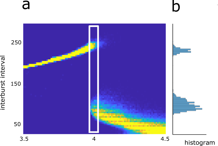
Figure 3: a. Histogram of the inter-burst interval for $\mu=0.01$ and various values of $\alpha$. A bimodal distribution, corresponding with slow chaos, arises in a non-trivial range of $\alpha$ in the vicinity of the crisis at $\alpha=4$ (white box). b. One typical histogram for $\mu=0.01$ and $\alpha=4$.

To further characterize the fluctuations of the deterministic dynamics on the order of the slow time scale, let us consider the sequence of interburst intervals along a given trajectory, as seen in Fig. 3a. A unimodal, non-Dirac distribution corresponds to fast chaos trajectories, with distributions centered at larger durations for fast chaos with no shortcut (cf. Fig.3a, small $\alpha$), and centered at smaller durations for fast chaos trajectories where the probability of shortcut is unity (cf. Fig.3a, large $\alpha$). In contrast, slow chaos corresponds to bimodal distributions of interburst intervals, corresponding to trajectories composed of both long bursts and shortcuts (inside the white box in Fig. 3a and in 3b).

The emergence of slow chaos can be further characterized by either the coefficient of variation $c_{v}$ for the interburst intervals (cf. Fig. 4a) or its timescale normalized standard deviation (cf. Fig. 4b). For small $\alpha$, this shows we have fast chaos. For $\alpha\approx 4$ we have slow chaos, and while the crisis in the fast subsystem occurs at $\alpha=4$, the emergence of slow chaos occurs at an $\mu$-dependent $\alpha$ value a bit less than $4$. The figure shows that for each $\mu$, the transition to slow chaos is quite rapid, and the $0.1$ level set (black line) serves as a good choice to define the transition point. As $\mu\to 0$, the $\alpha$-window with slow chaos shrinks to size zero. For $\alpha>4$ we have fast chaos again, since orbits reliably take the shortcut. Finally, for $\alpha\gg 4$ the relaxation cycle breaks down, and we have continuous bursting.

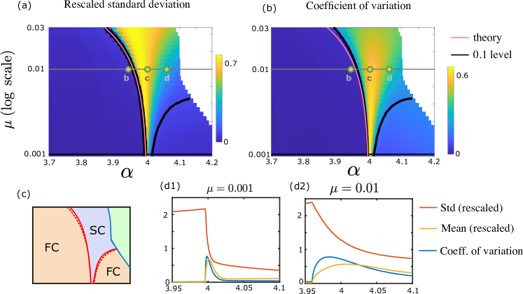
Figure 4: (a) Standard deviation rescaled by the parameter $\mu$. (b) Coefficient of variation $c_{v}$ of the interburst interval as a function of the parameters $\alpha$ and $\mu$. In both (a) and (b), we observe a sharp transition at the onset of slow chaos. The pink line depicts our theoretical derivation of the onset of slow chaos. The black line depicts the 0.1 level set for the corresponding measure. The location of the level sets is consistent with our theoretical prediction. The circles b,c,d indicate the parameter values from resp. Fig. 2b,c,d. (c) Bifurcation diagram of the system obtained from (a) and (b): FC: Fast Chaos (beige), SC: Slow Chaos (purple), and Loss of Relaxation cycles (green). Bifurcation Lines (red) are the 0.1 levels of rescaled $\bm{\sigma}$ (dashed) and $c_{v}$ (solid). (d1,d2) Depictions of the rescaled mean (yellow), rescaled standard deviation (red), and $c_{v}$ (blue) for $\mu=0.001$ (middle) and $\mu=0.01$ (right).

IV.2 Topological description

To present a topological description of how slow chaos emerges, we consider a coarse-grained representation of the dynamics Gedeon et al. (1999). Relaxation cycles in the $\mu\ll 1,\alpha<4$ regime consist of a concatenation of the following four dynamical sections (see Fig. 5d):

• Slow rise of the adaptation variable preceding a burst.

• Transition from quiescence to bursting.

• Bursting behavior with decay of the slow variable.

• Transition from bursting to quiescence.

However, for larger values of $\mu$ and $\alpha<4$ sufficiently close to $4$, we find that the slow dynamics may allow a return to the left stable fixed point through the emergence of short bursts (marked as T3 in Fig. 5d).

For $\alpha>4$, because of the presence of two $y$-values with crises, shortcuts exist for arbitrarily low values of $\mu$ between the two crisis $y$-values. In fact, shortcuts become the most likely outcome as $\mu\to 0$, and therefore coarse-grained transition graph must be slightly modified (Fig 5e). In that case, the transition region from bursting to quiescence is split into two disconnected pieces B2 and B3, with returns to quiescence denoted by T2 and T3. For $\mu$ sufficiently small, fast chaos occurs with relaxation cycle B1-T1-B2-T3, but when $\mu>0$, the transient chaotic behavior may prevent the system from undergoing transition T3; in this case, cycles transition to B3 through a new path B4, yielding a long bursting relaxation cycle B1-T1-B2-B4-B3-T2.

IV.3 Probabilistic model

Based on these observations, we have designed a probabilistic model to predict the emergence of slow chaos and estimate the shortcut probability (see Fig 5a). This model simply follows the Rulkov dynamics in the region of the phase plane where we expect non-chaotic branches of relaxation cycles (i.e., to the left of the unstable fixed point marked in yellow on the graph), and it randomly samples the support of the chaotic attractor otherwise.

More formally, our stochastic model approximates the fast chaotic dynamics with a random Bernoulli sequence (independent random variables) uniformly sampling the interval of possible values for the fast variable along a relaxation cycle. In particular, let $[Y_{0},Y_{1}]$ be the region of (slow variable) phase space where the transition $T3$ is accessible (cf. Fig. 5a), let $\mathcal{I}_{\mu}(y)$ be the interval of fast variable values during the high voltage portion of the burst, i.e. for which the fast dynamics are chaotic (red horizontal line in Fig. 5a), and define $\mathbb{U}_{I}$ to be a uniform random variable on this interval. Our model is given by:

$$\begin{cases}x_{n+1}=\begin{cases}\mathbb{U}_{\mathcal{I}_{\mu}(y_{n})}&Y_{0}<y_{n}<Y_{1}\;\text{and}\;x_{n}>u(y_{n})\\ F_{\alpha}(x_{n},y_{n})&\text{otherwise}\\ \end{cases}\\ y_{n+1}=y_{n}-\mu(x_{n}-\sigma)\;.\end{cases}$$

Here, $F_{\alpha}(x,y)=\frac{\alpha}{1+x^{2}}+y$ is the nonlinear fast dynamics, and $u(y)$ is the unstable fixed point of the fast dynamics.

Note that while an exact representation $\mathcal{I}_{\mu}(y)$ is only given implicitly, noting that the fast variable takes its maximum at $x=0$, this envelope is approximated by the first and second iterates of $x=0$, yielding a closed-form expression that closely matches the numerically observed support of the fast variable (see Fig. 5 b,c, black curves). The significance of this representation is that it provides a quantification of the relative occurrence of a shortcut between the two $y$ values associated with crisis points, where the deterministic chaotic system provides no information.

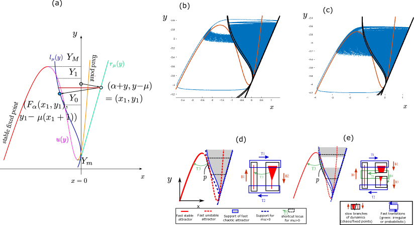
Figure 5: Probabilistic model and topological dynamics. (a) The dynamical structures and our approximation of the support of the fast attractor. This figure highlights the main notation used for the probabilistic model, in particular the left and right envelopes $l_{\mu}(y)$ and $r_{\mu}(u)$, the unstable fast equilibrium $u(y)$ and the possible intersections of the $l_{\mu}$ manifold and the unstable fast equilibrium manifold $Y_{0}$ and $Y_{1}$. The red horizontal line from $l_{\mu}(y)$ to $r_{\mu}(y)$ is $I_{\mu(y)}$. Panels (b) and (c) illustrate the slow chaos dynamics in the case of $\alpha<4$ (b) or $\alpha>4$ (c, specifically, $\alpha=3.98$ and $\alpha=4.02$, represented for $\mu=0.01$). Blue: trajectory, showing an excellent fit with the envelope computed analytically (black, outer curve; the inner black curve corresponds to $\mu=0$), Ref: fixed points of the fast system. (d-e) Cartoons of the dynamics and topological behavior. (d) slow chaos for $\alpha<4$ (here, $\alpha=3.98$ and $\mu=0.02$), where the support of the chaotic attractor does not intersect the unstable fast equilibrium but the slow variable may allow the system to take shortcuts $T_{3}$. (e) slow chaos for $\alpha>4$ (here, $\alpha=4.02$ and $\mu=0.02$) where shortcuts arise for arbitrarily small values of $\mu$, but for $\mu>0$ chaotic transients may allow jumping between the two parts of the chaotic attractor (transition $B_{4}$).

We now return in more detail to the slow-fast decomposition of the dynamics, using the dynamics of the fast variable $x$ (fast dynamics) when the slow variable $y$ is frozen. For each fixed $y$, this one-dimensional dynamical system is given by the function

$$x\mapsto F_{\alpha}(x,y)=\frac{\alpha}{1+x^{2}}+y.$$

The fixed points of this equation are thus the roots of the cubic polynomial:

$$x^{3}-x^{2}y+x-y-\alpha=0.$$

Therefore, depending on $y$ and $\alpha$, the system has between 1 and 3 solutions, corresponding to intersections of and fixed values of $y$ and the curve $y=x-\frac{\alpha}{1+x^{2}}$, forming the $x$-nullcline for the original map. In the case where there are three solutions, the middle fixed point is necessarily unstable and we denote it by $u(y)$, for a given $y$ and fixed $\alpha$ (cf. Fig. 5).

The fast dynamics $x\mapsto F_{\alpha}(x,y)$ is a unimodal map, and we observe numerically that increasing $\alpha$ leads to a period-doubling route to chaos, a classical result of a class of unimodal maps Yorke and Alligood (1985). To compute a region enclosing the chaotic attractor $\mathcal{I}_{\mu}(y)=\{x:l_{\mu}(y)<x<r_{\mu}(y)\}$, for each $y$, we estimate an upper-bound using the maximal value of $F_{\alpha}(\cdot,y)$, which is attained at $x=0$. Thus the graph of $r_{\mu}(y)$ is given by $\{(x_{1},y_{1})=(F_{\alpha}(0,y),y-\mu)=(\alpha+y,y-\mu):y\in\mathbb{R}\}$. The left side of the interval, meaning the graph of $l_{\mu}(y)$, is given by the image of the points $(x_{1},y_{1})$ on the graph of $r_{\mu}(y)$. That is, the graph of $l_{\mu}$ is given by

$$\{ ( \l_{\mu}(y_{2}),y_{2})=(F_{\alpha}(x_{1},y_{1}),y_{1}-\mu(x_{1}+1))$$ (3)

$$= (F^{2}_{\alpha}(0,y),y_{1}-\mu(x_{1}+1))$$

$$= \left(\frac{\alpha}{1+(\alpha+y)^{2}}+y,y-\mu-\mu(\alpha+y+1)\right):$$

$$y \in\mathbb{R}\}\,,$$

cf. the solid blue and green lines in Fig 5a, and show an excellent agreement with the simulations in Fig. 5d,e.

We know that the sequences of iterates will be contained in this interval as long as $F_{\alpha}(\mathcal{I}_{\mu}(y),y))\subset\mathcal{I}_{\mu}(y_{1})$, which is in particular the case when $l_{\mu}(y)$ is to the left of $u(y)$. Moreover, if $x=0$ belongs to the support of a chaotic attractor, then this support contains the boundaries of the interval $\mathcal{I}_{\mu}(y)$. In this situation, an internal crisis will arise for parameters and a slow variable $y$ such that $l_{\mu}(y)$ falls exactly on $u(y)$. The two points at which this occurs are $Y_{0}$ and $Y_{1}$ depicted in Fig. 5a. In the case $\mu=0$, the condition yields

$$2y^{2}+3\alpha y+\alpha^{2}+2=0\;.$$

and the roots of the equation are given $\frac{1}{4}(-3\alpha\pm\sqrt{\alpha^{2}-16})$, with two real roots when $\alpha>4$ (and a single real root at $\alpha=4$). Thus the chaotic attractor is contained in an interval tangent to $u(y)$. Two real solutions correspond to the two internal crises delineating the region of occurrence of slow chaos within $y\in[Y_{0},Y_{1}]$. Note that if $\alpha>4$ and $\mu>0$, but sufficiently small, then there will still be two ($\mu$-dependent) points $Y_{0}$ and $Y_{1}$ of intersection between $l_{\mu}(y)$ and $u(y)$. We will see below that in fact for small fixed $\mu>0$, the interval $[Y_{0},Y_{1}]$ persists for a small region of $\alpha<4$.

IV.4 A uniform random variable on the support

In the model introduced in the the previous section, for $y\in[Y_{0},Y_{1}]$, we have modeled the system such that it uniformly samples the region $\mathcal{I}_{\mu}(y)$ as it moves down along the slow flow, where we consider the fraction of length of the interval $\mathcal{I}_{\mu}(y)$ to the left of $u(y)$. This provides an approximate probability for each the iterate to lead to a shortcut trajectory. The probability of a long burst is thus given by the probability of never falling to the left of $u(y)$, which can be readily quantified.

In our stochastic model, the number of steps performed within the region $y\in[Y_{0},Y_{1}]$ varies inversely proportionally to $\mu$. For $\alpha>4$, since the interval $[Y_{0},Y_{1}]$ always contains the set of values of slow variables for which $\mathcal{I}_{0}(y)$ is to the left of $u(y)$, the probability of a short burst increases as $\mu$ is decreased. In contrast, for $\alpha<4$, decreasing $\mu$ enough will eventually prevent any intersection between $\mathcal{I}_{\mu}(y)$ and $u(y)$ for all $y$, because of the continuous dependence upon parameters and the fact that there is no intersection with $\mathcal{I}_{0}(y)$.

We thus expect that, if $\mu$ is sufficiently close to 0, the probability of a short burst will suddenly jump from 0 and 1 at $\alpha=4$. This is visible in Fig. 6, where we show the joint dependence of the probability of a short burst in $\alpha$ and $\mu$ (computed with numerical integration).

Let us now use this probabilistic model to estimate the alternation of shortcuts and long bursts for a fixed value of $\mu$. If the attractor never intersects the unstable fixed point (i.e., $l_{\mu}(y)>u(y)$ for all $y$ where both functions are defined), long bursts arise systematically, and the system displays fast chaos. However, if there exists an interval of values $y\in[Y_{0},Y_{1}]$ such that $l_{\mu}(y)<u(y)$, an iterate of the stochastic system leads to a shortcut with “instantaneous” probability $\rho_{\mu}(y)=(u(y)-l_{\mu}(y))/(r_{\mu}(y)-l_{\mu}(y))$. The probability of not taking the shortcut per burst will thus be given by the product of $\prod_{n=n_{0}}^{n_{1}}(1-\rho_{\mu}(y_{n}))$ where $n_{0}$ is the time $y_{n}$ enters $[Y_{0},Y_{1}]$, and $n_{1}$ is the exit time.

While this can be computed explicitly, we further simplify the problem by considering an averaged shortcut probability computed as the fraction of surface area $p$ to the right of the unstable fixed point (green region in Fig. 5d,e), and the number of iterates is estimated as $N=(Y_{1}-Y_{0})/\mu$, the probability of a long burst is $P_{l}=(1-p)^{N}$. Numerical calculation of $p$ under this assumption shows very good agreement with the original simulations of the Rulkov model as we show in Fig. 6. Going further, we observe that the exponential dependence in $1/\mu$ makes the probability switch from $0$ to $1$ very rapidly upon variation of the time scale parameter $\mu$ at a given value of $\alpha$ (i.e., for $p$ fixed). This indicates that in the limit of timescale separation, the system always displays fast chaos, with long bursts for $\alpha<4$ and short bursts for $\alpha>4$. As $\mu$ is decreased, slow chaos occurs on a smaller interval of $\alpha$, as shown in Fig. 4. This approach provides a very accurate value, for $\mu>0$, of the emergence of slow chaotic trajectories for typical $\alpha<4$, as seen by comparing the solid and dashed lines in Fig. 6. For any fixed value of $\alpha$, there exists $\mu$ sufficiently small for which the system displays fast chaos only, characterized by relaxation oscillations.

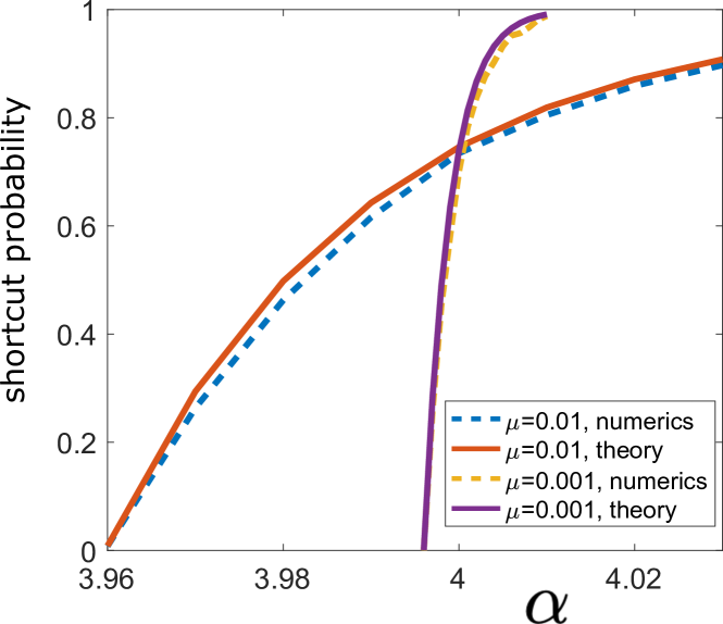
Figure 6: Slow chaos and probabilistic model. The shortcut probability simulated shows an excellent agreement with our analytical expression for the probabilistic model.

The fine analysis above is made possible by the simplicity of the Rulkov map, but it also reveals a robust phenomenon: relaxation cycles through fast chaotic attractors will yield mathematically chaotic behaviors that appear regular at larger timescales, and these phenomena will breakdown at internal crises of chaotic attractors where chaotic alternations of longer and shorter cycles will emerge. To provide further evidence that this occurs for fast slow systems with attractor crises, subsequent sections demonstrate that the same behavior occurs in three other models: a network model of the Rulkov map with the topology of the crab STG (Sec. V), a cubic discrete dynamical showing a double crisis (Sec. VI.1); and a 5-dimensional FitzHugh-Nagumo neuron model coupled with the Lorenz system at a fast timescale (Sec. VI.2).

V Network of Rulkov maps and Central Pattern Generators

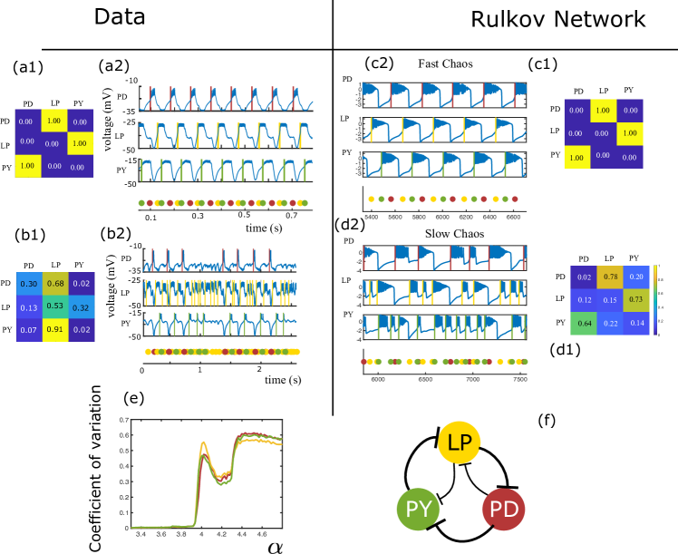
Figure 7: Left: experimental data from Kedia and Marder (2022). Right: simulations of a three-neuron Rulkov model with inhibitory connectivity mimicking the pyloric network, with architecture depicted in panel (f). (a) Intact network, (b) Decentralized biological network with irregular activity, (c) Rulkov model in the fast chaos regime ($\mu=0.01$, $\alpha=3.8$) and (d) Rulkov model in the fast chaos regime. ($\mu=0.01$, $\alpha=4$). (a2,b2,c2,d2): Voltage traces for each neuron with, on the bottom, a stop-light representation of the spike sequence. The associated transition matrices are shown in (a1,b1,c1,d1). The coefficients of variations for the depicted trajectories are: (a2) 0.01, (b2) 0.60, (c2) 0.02, (d2) 0.62, and the evolution of the coefficient of variation for each population (same color code), depicted in panel (e), shows a clear transition slightly before $\alpha=4$ from low levels associated with fast chaos to large levels associated with slow chaos.

We next explore the dynamics of a simple phenomenological model of the crab STG made of three identical chaotic Rulkov neurons with a biologically-inspired connectivity map (see Fig. 7, right). Specifically, the connectivity parameters are chosen randomly as

$$\left(\begin{array}[]{ccc}0&-5.5&-2.5\\ -3.5&0&-5\\ -3&0&0\end{array}\right)+U\,,$$

where $U$ is a random matrix with off-diagonal elements chosen from a uniform distribution between $[-0.5,0.5]$, and zeros on the diagonal. Of course, the neural network of the central pattern generators of the crab discussed in the introduction involve neurons with vastly richer dynamics than the Rulkov map and with heterogeneous properties. The present model allows us to test the relevance of the transition to slow chaos in a network without complications associated with intrinsic dynamics or heterogeneities, although this would be a simple extension of our analysis.

We compared our model in the regime of fast chaos and slow chaos to two typical sequences recorded experimentally in the crab STG (data from Kedia and Marder Kedia and Marder (2022)) that qualitatively corresponded to fast chaos (intact network Fig. 7a) or slow chaos (decentralized network Fig. 7(b). We simulated our network and tested for the sequence of neurons spiking, deemed to be biologically relevant information. For that purpose, we identified the onset of each burst and extracted the sequence of burst initiations (colored circles below the neural dynamics traces) identified using a threshold-crossing condition (thresholds were adjusted according to the experimental traces for each neuronal type, and fixed to $-1.5$ for the model), which led to the stop lights dynamics represented below the traces. This sequence of spikes was used to construct a “transition probability matrix” $M$ that contains as element $M_{ij}$ the empirical frequency that neuron $j$ spikes after neuron $i$. This is a stochastic matrix, since all elements are non-negative and the sum over all columns on a given line is equal to $1$. Given these matrices, we further computed an entropy level, computed as the average entropy of each line, or $-\frac{1}{3}\sum_{i,j}M_{ij}\log(M_{ij})$ with the convention that $x\log(x)=0$ for $x=0$. A deterministic sequence gives an entropy equal to $0$, while a maximal entropy of $\log(3)\approx 1.0986$ corresponds to a completely random sequence of spikes.

We compared our model in the regime of fast chaos and slow chaos to two typical sequences that correspond to fast chaos vs slow chaos recorded experimentally Kedia and Marder (2022). We observed that both cases of fast chaos are certainly regular enough to ensure a fully predictable sequence of spikes with probability 1 for the next spike neural population to spike, and thus entropy zero. However, the typical trace of a slow chaos experimental data shows a very irregular sequence, with evidence of the presence of shortcuts (shorts bursts) very evocative of those observed in the Rulkov model (see left column, bottom). This is further shown in the coefficient of variation of the network as a function of $\alpha$, showing a sudden jump from small fluctuations to larger values arising again in the vicinity of $\alpha=4$ where we showed the emergence of a crisis in the Rulkov map. The experimental dynamics (left) are quite comparable to the network model we designed, and in particular the transition matrix in this regime is non-trivial, with strictly positive probabilities to have any neuron spiking after any other neuron, non-trivial entropy (0.67 for the data, 0.75 for the model) and larger coefficients of variations of interburst intervals (see Fig. 7(e)).

VI Crises yield transitions between slow and fast chaos in other chaotic slow-fast models

To further explore the generality of our observation of dynamical structures underlying fast chaos and their transitions to slow chaos, we explore two other examples of multiple timescales dynamical systems, illustrating that our results are indeed not specific to a single system, and rather occur in a variety of slow-fast systems with crises, both in discrete-time maps and differential equations.

VI.1 Cubic map

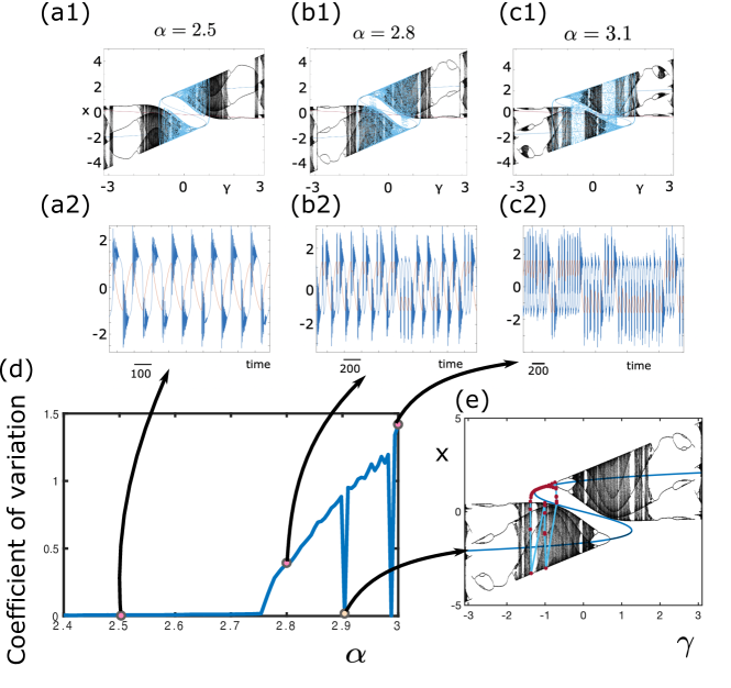
Figure 8: Cubic map simulations for $\alpha\in\{2.5,2.8,3.2\}$, illustrating respectively fast chaos and a transition to slow chaos as the system approaches and crosses the crisis in the fast system (arising at $\alpha=3$). Top: phase space, with the fast attractor for various values of $\gamma$ (black) as well as the trajectory of the system for $\varepsilon=0.01$ (cyan). Middle: evolution of the fast variable $x$ (blue) and slow variable $\gamma$ (orange) as a function of the iterate number, illustrating clearly the emergence of fast chaos whereby macroscopically regular but microscopically chaotic behaviors emerge, and their transition to slow chaos with irregular dynamics when shortcuts in the relaxation cycles can arise during transient chaos near crises. Bottom: the coefficient of variation of the system as a function of $\alpha$ shows a sudden increase at the emergence of slow chaos, with sudden drops associated with the emergence of periodic orbits (bottom right, for $\alpha=2.904$).

In Han et al. (2017), a one-dimensional, three-parameter cubic map was introduced and shown to feature complex dynamics. This system is given by the equation:

$$x_{n+1}=(-\beta x_{n}^{3}+\alpha x_{n}+\gamma)\,.$$

It has been shown to display chaos for specific values of the parameter $\gamma$ with or without internal crises depending on the value of $\alpha$. We exploit this dynamical richness to explore the existence of fast and slow chaos and the transitions between the two regimes. To this purpose, we extend the system to allow slow autonomous variation of $\gamma$, with linear dynamics according to $x$, in such a way that the system will tend to produce relaxation cycles through the chaotic attractors:

$$\begin{cases}x_{n+1}&=(-\beta x_{n}^{3}+\alpha x_{n}+\gamma_{n})\phi(x_{n})\\ \gamma_{n+1}&=\gamma_{n}+\varepsilon(-\kappa\gamma_{n}-x_{n}+\delta-\mu x_{n}^{3}).\end{cases}$$

In the equations above, we added for stability of the system a cubic term $-\mu x^{3}$ to the linear dynamics of $\gamma$ and a multiplicative term $\phi(x_{n})$ to the $x$-dynamics preventing divergences when $x$ is large. Here, $\phi$ is a smooth function with a plateau equal to 1 and decaying to zero as $|x|\to\infty$ . Parameters are fixed to $\beta=0.5$, $\kappa=0.1$, $\delta=0.2$, and $\mu=0.9$. (These parameters were chosen arbitrarily to ensure the creation of appropriate relaxation cycles given the cubic dynamics.) The timescale of the evolution of $\gamma$ is governed by the parameter $\varepsilon$ and has been set to $0.01$ in our figure. For these parameters, the fast variable typically displays chaos for appropriate values of $\gamma$. The fast variable features hysteresis between two stable fixed points for $1<\alpha<2$, which is associated with standard relaxation cycles for the full system.

Chaos emerges on both branches at $\alpha=2$, and initially, these fast chaotic trajectories are confined above or below the unstable fixed point. In that configuration, consistent with our analysis of the Rulkov system, we observe fast chaos, with regular relaxation cycles that include a passage through a chaotic attractor (Fig. 8a1) and hysteresis between chaotic attractors starting from $\alpha=2$, associated with fast chaos trajectories with a relatively regular slow dynamics (red curve, Fig. 8a2) and fast trajectories that show chaos at a fast timescale but almost periodic behavior at the slow timescale. To identify the duration of each relaxation cycle, we used a threshold-crossing condition. We computed, for each value of the parameters, the location of the saddle-node bifurcations of the fast variable. We chose the leftmost fold and identified one relaxation cycle by considering times when the fast variable when from behind larger to smaller than this value and with the slow variable being below the value of $\gamma$ associated. For $\alpha=2.5$ as in Fig. 8a, we found a coefficient of variation equal to $0.008$, indicating that the period of relaxation cycles fluctuates by less than 1%, corresponding to a clear instance of fast chaos.

As $\alpha$ is increased, the chaotic attractors of the fast system approach the unstable fixed point, until both of them hit the unstable fixed point curve tangentially for $\alpha=3$ at a double-crisis (the coincidence of the two crises is associated with the symmetry of the system). This bifurcation determines the breakdown of fast chaos and the emergence of slow-chaos trajectories. For the full slow-fast system, similar to the case of the Rulkov map, we observe that slow chaos emerges a little before the value of $\alpha=3$ due to the dynamics of the slow variable (according to Fig. 8d, at around $\alpha=2.76$, and this value shall approach $3$ as $\varepsilon$ is decreased). At $\alpha=2.8$ we clearly observe slow chaos with irregular slow dynamics (red curve in Fig. 8b2, coefficient of variation $0.311$) associated with whether or not, during the chaotic transient associated with the region of values of $\gamma$ between the two crises, the trajectory crosses the unstable fixed point short-cutting the relaxation or performs a long relaxation cycle, which persists as $\alpha$ is further increased (for $\alpha=3$, Fig. 8c1-c2 show the presence of slow chaos with a coefficient of variation $1.184$).

We note that our systematic computation of the coefficient of variation as a function of $\alpha$ also included sudden drops to a standard deviation of zero. We selected one of these points (here, $\alpha=2.904$, Fig. 8e) and observed that for this particular parameter value, the system converged towards a periodic orbit of period 37 instead of performing relaxation cycles.

VI.2 FitzHugh-Nagumo-Lorenz model

A natural question that could arise at this stage is whether the alternation of short and long bursts in the Rulkov map or the cubic map could be associated with the discrete nature of the dynamics, and would disappear in differential equations. To explore this question numerically, we designed a differential equation that couples relaxation cycles and chaos. The slow-fast systems discussed above are both non-invertible two-dimensional maps. Thus to see the same behavior in a differential equation, one would expect to need at least a four-dimensional model. (In fact, the model we constructed is five-dimensional, but we expect four dimensions would suffice.) We constructed our system by coupling two classical models: the FitzHugh-Nagumo neuron model FitzHugh (1955, 1961); Nagumo et al. (1962) well-known to produce relaxation cycles (variables $(r,h)$ in our equations); and the celebrated Lorenz system, well known to produce chaotic trajectories Lorenz (1963) (variables $(x,y,z)$). We coupled these systems by using the slow variable of the FitzHugh-Nagumo system as a bifurcation parameter of the Lorenz system. In that way, as the FitzHugh-Nagumo variables perform a relaxation cycle, the Lorenz system will go in and out of its chaotic regime. We used a single Lorenz variable ($x$) as an input to the FitzHugh-Nagumo fast variable, rescaled by a coefficient $\delta$. For small $\delta$, the chaotic fluctuations of the Lorenz equation will have a smaller impact on the FitzHugh-Nagumo dynamics, while for a large $\delta$, the impact will be more substantial and may break down the relaxation cycles. The resulting system of equations is given by:

$$\begin{cases}\dot{x}&=\sigma\,(y-x)\\ \dot{y}&=-x\,z+\gamma\,(\nu+r)\,(\nu+x)-y\\ \dot{z}&=x\,y-b\,z\\ \\ \dot{h}&=h-h^{3}/3-r+\delta x\\ \dot{r}&=\varepsilon\,(h-r)\,.\end{cases}$$ (4)

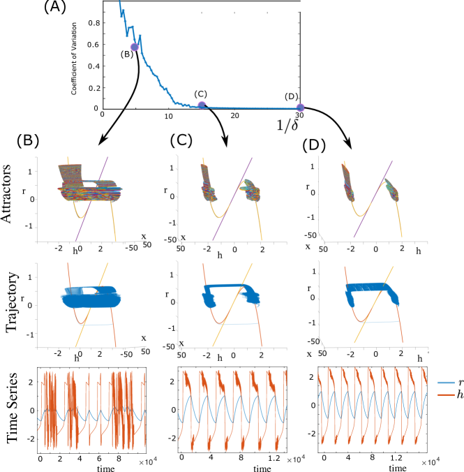
Figure 9: Simulations of the FitzHugh-Nagumo Lorenz model, for $\delta=3$ (top, a1,b1,c1) or $\delta=30$ (bottom, a2,b2,c2). Left: fast attractors, where each color represents a distinct orbit (a1,a2), Middle: projection of the five-dimensional trajectory of the system in the space $(r,h,x)$ (b1,b2) and Right: time-evolution of the FitzHugh-Nagumo variables $r$ and $h$ (c1,c2).

The parameters $\gamma$ and $\delta$ are scaling parameters that control the amplitude of the coupling of those equations, with $\gamma$ fixed equal to $400$ allowing us to generate our type of dynamics, an $\delta$ being varied. The parameter $\varepsilon=0.01$ is the slow timescale ratio, and the Lorenz system parameters are fixed to $\sigma=10$ and $b=2.66$ throughout our simulations. By design, the Lorenz system will generate fast chaotic dynamics when the slow variable of the FitzHugh-Nagumo model $r$ is large enough, which induces chaotic dynamics of the fast variable $h$. The parameter $\delta$ controls the amplitude of the fast dynamics chaotic attractor, and it can be chosen to induce an internal crisis. For $\delta=1/30$ the chaotic attractors are significantly scaled-down and remain far from the unstable fixed point (Fig. 9D), and the system generates relatively regular relaxation oscillations through the chaotic attractors, corresponding to fast chaos. To estimate the fluctuations in the period of the relaxation cycles, we have used a Poincaré section placed on the hyperplane $h=0$ and recorded the crossings associated with $h$ increasing and $r<-0.2$. This condition was found to capture precisely the relaxation cycles away from the chaotic behaviors. For $\delta=1/30$, we confirmed that the fluctuations in the duration of the relaxation cycles were very small compared to the mean, with a coefficient of variation $c_{v}=0.01$.

As $\delta$ increases, we observe that the coefficient of variation transitions from small values to significantly larger values, as the fast attractor dynamics grows, generating a crisis and opening the way to shortcut trajectories. These are visible in particular for $\delta=1/4$ (Fig. 9B), where the fast attractor clearly shows the presence of two crises that open a shortcut avenue. Associated relaxation cycles show an erratic alternation between trajectories that perform a full relaxation cycle and those that transition earlier.

VII Discussion

In this paper, we demonstrate that while chaos is usually associated with disorder, the relationship between macroscopic patterns and chaos can be more complex, and in particular mathematically chaotic systems can display regular and robust dynamics at slow timescales. We have shown that the presence of external crises of chaotic attractors combined with relaxation cycles predicted the existence of sharp transitions between such relatively regular chaotic dynamics and erratic behaviors at slow timescales. In these regimes, erratic alternations between long and short bursts are governed by long irregular transients around the ghost of a chaotic attractor, a scenario that we sharply validated with the introduction of a purely probabilistic model from which we predicted the frequency of occurrence of shorter bursts. Both slow and fast chaos are phenomena that arise in a variety of maps and continuous systems. We showed that the coefficient of variation associated with a time series of interburst intervals (or some other appropriately chosen observable associated with the slow dynamics) robustly distinguishes between slow and fast chaos in a variety of scenarios, even including intracellular voltage data. Our models yield dynamics very similar to what is observed experimentally in the crab nervous system. We further illustrate this with a 3-neuron model and various quantifications of data and numerical simulations.

This phenomenon adds to a wide literature on chaotic dynamics of neural systems, that finely characterized micro- and macro-chaotic structures in bifurcation diagrams Barrio et al. (2014) and the fine dynamics of chaotic alternations in bursts at spike-adding transitions in slow-fast systems of bursters Barrio et al. (2021); Medvedev (2006); Serrano et al. (2021), with a possible key role of canards Shilnikov and Rulkov (2003). Remarkable works also carefully investigated the complex chaotic dynamics of models of pancreatic beta-cells systems Duarte et al. (2009), and argued that another global bifurcation called interior crises of chaotic attractors could be related to some sudden changes in bursting behaviors Duarte et al. (2017).

This paper is focused on deterministic chaos as a source of variability. Another interesting perspective of this work is the question of the robustness of slow behaviors in stochastic systems and their breakdown. A first observation is that the observations made in the Rulkov map persisted in stochastic systems with small Gaussian additive noise: even if theoretically shortcuts and changes of the period are allowed with Gaussian noise, these occurred with rare probability, before the crisis, and suddenly became much more frequent as the system approached the deterministic crisis (see Figure 10).

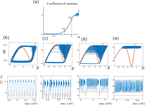
Figure 10: Simulations of the Rulkov map with additive Gaussian noise on the voltage variable $x_{n+1}=\frac{\alpha}{1+x_{n}^{2}}+y_{n}+\gamma\xi_{n}$, $y_{n+1}=y_{n}-\mu\;(x_{n}-\sigma)$, with $\gamma=0.05$ and $(\xi_{n})_{n\geq 0}$ independent standard Gaussian random variables. (a): coefficient of variation computed for $N=10^{7}$ iterates after a transient of $10^{5}$ iterates, with events computed as in Figure 4. (b-e) trajectories in the phase plane (top) or as a function of time (bottom) for $\alpha=2.7$(b), $\alpha=3.8$ (c), $\alpha=4$ (d) and $\alpha=5$ (e).

In stochastic systems however, chaos is not needed to generate irregular behaviors and therefore such transitions between fast and slow chaos may rely on a variety of other types of dynamical and stochastic structures that would allow sudden switches in the probability distribution of first passage times. The study of these systems and structures open some new avenues of investigation.

Appendix

This Appendix gives a couple of details that are tangential to the main text. Section A gives a detailed description of the crustacean STG with data shown in Fig. 1. Section B qualitatively classifies the different types of chaos observed in the Rulkov map. Section C discusses computational methodologies used for the FitzHugh-Nagumo-Lorenz model.

Appendix A A detailed description of the STG model

The stomatogastric ganglion (STG) of crustaceans is a well-studied rhythmic motor circuit that controls movements of muscles involved in chewing and filtering of food. It produces a remarkably stable output in the face of changing internal and external conditions and has provided deep insights into the circuit and cellular-level mechanisms involved in achieving circuit robustness and homeostasis. The pyloric circuit within the STG is a central pattern generator that produces a characteristic triphasic pattern of activity. A pair of pyloric dilator (PD) neurons bursts initiate the rhythm, and they are followed in phase by a lateral pyloric (LP) neuron and finally by the pyloric neurons (PYs). All neurons have large amplitude slow-wave membrane voltage oscillations and fire a burst of action potentials at the peak of the depolarization during normal activity (Fig. 1a ). There is cycle-to-cycle variability of minor features of this pattern, but the order of firing, relative phases, and duty cycles (fraction of the cycle period during which a neuron is firing) are key to maintaining a functional output and are invariant. Upon blocking of the neurohormonal inputs to the STG (decentralization), this rhythmic bursting activity can change to an erratic spiking behavior with sporadic bursts and a complete loss of rhythmicity. The circuit is no longer functional in this state (Fig.  1b). From the mathematical viewpoint, STG circuit activity shows hallmarks of chaos both in the rhythmic and non-rhythmic conditions, as shown in the transition probability analysis plots in the bottom row of Fig. 1. Cycle-to-cycle variability of the spikes within a given burst, especially in LP and PY spikes can be seen, which fills a region of space in the three-variable plot even during normal triphasic activity.

Appendix B Classification of chaotic behaviors

The main text concentrates on distinguishing between fast and slow chaos, two qualitative behaviors that appear most meaningful for qualitative descriptions. Our analyses led us to further identify the following types of chaotic behaviors:

Weak chaos. For a region of $\alpha$ values starting around $2.7$ we observe a phenomenon we refer to as weak chaos cf. Fig. 2a in which the system is detected as chaotic using several measures of chaos, but does not noticeably alter the overall dynamics or functionality. The underlying mechanism for this chaos appears to be referred to as a weakly chaotic ring in Mira and Shilnikov (2005), the same as the phenomenon found in Lorenz (1989).

After $\alpha$ reaches the value $3$, the fast subsystem exhibits bistability, with a stable fixed point less than the resting membrane potential $\sigma$, and a chaotic attractor mostly located above $\sigma$. Again, the time trajectories are not significantly altered in terms of functionality.

Fast chaos. Starting at around $\alpha>3.5$, the system shows relaxation oscillations through the strange attractor of the fast variable, cf. Figs. 2b. However, the decay of the slow variable takes a relatively fixed time. Thus the interburst intervals appear periodic at the slow timescale and the chaos is restricted to fast timescales.

Slow chaos. As $\alpha$ is increased towards 4, as in Fig. 2c, the full system escapes the chaotic region through a new route, or shortcut, distinct from the classical relaxation cycle. The plot of the slow variable shows that it is unpredictable whether the escape from chaos will be through the classical or shortcut route. Slow chaos persists for $\alpha>4$, as in Fig. 2d. However, the frequency of the shortcut becomes greater as $\alpha$ increases. Since slow chaos results in unpredictable interburst intervals, slow chaos results in loss of functionality. Terman Terman (1992) described slow chaos and symbolic dynamics in a neural model with relaxation cycles as a system transitions from periodic bursting to spiking, but the mechanism is different and does not include the possibility of fast chaos.

Hyperchaos. When $\alpha$ is sufficiently away from the crisis, the frequency at which the system describes a full relaxation cycle vanishes, and the system fires repetitively without returning to the resting potential, cf. Figs. 2e. The dynamics at $\alpha$ above around $4.5$ displays hyperchaos, since it has two positive Lyapunov exponents, cf. Fig. 2 bottom; see Rössler (1979); Stankevich et al. (2021).

Appendix C Computational Methodologies

All of our numerical simulations were performed using code written in Matlab. The source code for all numerical simulations is available at Jaquette et al. (2023).

Simulations of the continuous time FitzHugh-Nagumo-Lorenz model were performed in Matlab using the ode45 integrator with relative tolerance $10^{-5}$ and absolute tolerance $10^{-7}$. The trajectories for the 3 examples provided were confirmed using the routines ode113, ode15s and ode23s, or with lower tolerances, and we observed no qualitative difference in the trajectories. Solutions were computed over $250\,000$ time units. Fast attractors were computed similarly over a range of values of $r$ considered fixed, and starting with a range of initial conditions in the vicinity of the fixed points of the fast system (fixed points were computed using the Matlab vpasolve function and initial conditions were drawn randomly according to a Gaussian centered the fixed point with standard deviation 0.01.

References

- Hayashi and Ishizuka (1992) H. Hayashi and S. Ishizuka, Journal of Theoretical Biology 156, 269 (1992).
- Korn and Faure (2003) H. Korn and P. Faure, Comptes rendus biologies 326, 787 (2003).
- Kedia and Marder (2022) S. Kedia and E. Marder, Current Biology 32, 1439 (2022).
- Bernard (1879) C. Bernard, Leçons sur les phénomènes de la vie commune aux animaux et aux végétaux, Vol. 2 (Baillière, 1879).
- May et al. (1998) M. J. May, T. Vernoux, C. Leaver, M. V. Montagu, and D. Inzé, Journal of Experimental Botany 49, 649 (1998).
- Dijk et al. (1999) D.-J. Dijk, J. F. Duffy, E. Riel, T. L. Shanahan, and C. A. Czeisler, The Journal of physiology 516, 611 (1999).
- Aronoff et al. (2004) S. L. Aronoff, K. Berkowitz, B. Shreiner, and L. Want, Diabetes spectrum 17, 183 (2004).
- Turrigiano and Nelson (2004) G. G. Turrigiano and S. B. Nelson, Nature reviews neuroscience 5, 97 (2004).
- Cannon and Miller (2016) J. Cannon and P. Miller, Journal of neurophysiology 116, 2004 (2016).
- Marder and Tang (2010) E. Marder and L. S. Tang, Neuron 66, 161 (2010).
- Naudé et al. (2013) J. Naudé, B. Cessac, H. Berry, and B. Delord, Journal of Neuroscience 33, 15032 (2013).
- Goldberger (1991) A. L. Goldberger, Physiology 6, 87 (1991).
- Reed et al. (2017) M. Reed, J. Best, M. Golubitsky, I. Stewart, and H. F. Nijhout, Bulletin of mathematical biology 79, 2534 (2017).
- Golubitsky and Stewart (2018) M. Golubitsky and I. Stewart, SIAM Journal on Applied Dynamical Systems 17, 1816 (2018).
- Golubitsky and Wang (2020) M. Golubitsky and Y. Wang, Journal of mathematical biology 80, 1163 (2020).
- Yu and Thomas (2022) Z. Yu and P. J. Thomas, Journal of Mathematical Biology 84, 1 (2022).
- Marder and Bucher (2007) E. Marder and D. Bucher, Annu. Rev. Physiol. 69, 291 (2007).
- Alonso and Marder (2020) L. M. Alonso and E. Marder, Elife 9, e55470 (2020).
- Alonso and Marder (2019) L. M. Alonso and E. Marder, Elife 8 (2019).
- Sander and Yorke (2015) E. Sander and J. A. Yorke, International Journal of Bifurcation and Chaos 25, 1530011 (2015).
- Jaquette et al. (2023) J. Jaquette, S. Kedia, E. Sander, and J. D. Touboul, Codes of “Reliability and robustness of oscillations in some slow-fast chaotic systems”, https://github.com/JCJaquette/Slow-Fast-Chaos (2023).