Thermodynamic measurement of non-equilibrium stochastic processes in optical tweezers

Abstract

Due to their versatility in investigating phenomena in microscopic scales, optical tweezers have been an excellent platform for studying stochastic thermodynamics. In this context, this work presents experimental measurements of the energetic cost of driven finite-time protocols using colloidal Brownian particles in harmonic potentials. For this simple model system, we compare the results of optimal and sub-optimal protocols in a time-dependent trap, controlling the trap stiffness with different modulation amplitudes and protocol times. We also calculate the Jarzynski relation for the stochastic trajectories from the experimental data as an independent consistency check.

I Introduction

In classical thermodynamics, when one changes the state of a system in contact with a thermal reservoir, the minimum amount of work necessary to perform a process between the states is given by the Helmholtz free energy difference. This efficiency, however, is only achieved when performing the process quasistatically, i.e., with a protocol time that tends to infinity. For any finite-time tasks, the energy cost depends on the system’s trajectory in the phase space and, for a given set of parameters, there is a protocol that minimizes the energy dissipation. This is called the optimal protocol.

Although finding an analytic solution can be challenging in the general case, there are a few known results seifert ; Gomez-Marin ; Schmiedl2 and methods for obtaining approximate optimal protocols in different regimes, as for slowly varying processes and weak processes Bonanca1 ; Bonanca2 ; Large ; kamizaki ; kamizaki2 . These results, allied to the evolution of experimental techniques otani , allow one to study this subject using optical tweezers in current laboratories and increasingly contribute to understanding biological systems’ processes and the limits of energetic and informational efficiencies. In particular, identifying optimal protocols is of pivotal importance for designing highly efficient heat engines martinez2017 .

In this scenario, we investigate the experimental verification of analytical results obtained by Schmiedl and Seifert seifert , which explore the optimization of processes applied to overdamped colloidal particles trapped in a harmonic potential.

II Stochastic thermodynamics and optimal protocols

Considering a Brownian particle initially in thermal equilibrium, we can describe its one-dimensional dynamics using the Langevin equation in the overdamped limit:

$$\gamma\dot{x}=-\frac{\partial V(x,\lambda(t))}{\partial x}+\zeta,$$ (1)

where $\zeta$ represents the noise related to the thermal fluctuations, considered to be a Gaussian white noise; $\gamma=6\pi\eta a$ is the particle friction coefficient, with $\eta$ being the medium viscosity and $a$ the particle radius, and $V(x,\lambda(t))$ is the potential dependent on the coordinate $x$ and the control parameter $\lambda(t)$.

Sekimoto sekimoto showed in the late 90s that thermodynamic quantities such as work, $W$, and heat, $Q$, can be associated with the stochastic trajectories of colloidal particles. Therefore, by using the Langevin equation, we have:

$$-\left(-\gamma\frac{dx(t)}{dt}+\sqrt{2k_{B}T\gamma}\zeta(t)\right)dx+dV=\frac{\partial V(x,\lambda)}{\partial\lambda}d\lambda.$$ (2)

The first term on the left-hand side, identified as heat, is a result of the exchange of the particle’s energy with the medium, and the right-hand side term represents the stochastic work. Here, $k_{B}$ is the Boltzmann constant, and $T$ is the temperature.

Thus, changing the control parameter from $\lambda_{i}$ to $\lambda_{f}$ in a finite protocol time $\tau$, the stochastic work is equal to

$$W=\int_{0}^{\tau}d\tau\dot{\lambda}\frac{\partial V}{\partial\lambda}.$$ (3)

Since fluctuations are crucial in this regime, due to the inherent stochasticity of small systems, the optimal protocol is the one that minimizes the average work, $\langle W\rangle$.

Schmiedl and Seifert found analytical solutions for optimal protocols in time-dependent harmonic potentials, changing the trap’s stiffness and central position seifert . However, this article constrains the discussion to the case of controllable trap stiffness. Hence, for this case, the external potential can be simply written as:

$$V(x,t)=\frac{\lambda(t)x^{2}}{2}.$$ (4)

According to ref. seifert , the finite-time optimal protocol, $\lambda^{*}(t)$, that minimizes the average work, $\langle W\rangle$, is:

$$\lambda^{*}(t)=\frac{\lambda_{i}-c_{2}^{*}\gamma(1+c_{2}^{*}t)}{(1+c_{2}^{*}t)^{2}},$$ (5)

where

$$c_{2}^{*}=\frac{-\gamma-\lambda_{f}\tau+\sqrt{\gamma^{2}+2\lambda_{i}\tau\gamma+\lambda_{f}\lambda_{i}\tau^{2}}}{\tau(2\gamma+\lambda_{f}\tau)}.$$ (6)

Also, the average work in this process is given by

$$\langle W\rangle=\frac{\lambda_{f}}{2\lambda_{i}}(1+\tau c_{2}^{*})^{2}+\frac{(\tau c_{2}^{*})^{2}\gamma}{\lambda_{i}\tau}-\frac{1}{2}-\ln(1+c_{2}^{*}\tau).$$ (7)

This protocol, as shown in Fig. 1, implies discontinuities in $t=0$ and $t=\tau$, since $\lambda(0)\neq\lambda_{i}$ and $\lambda(\tau)\neq\lambda_{f}$, and depends basically on the amplitude of modulation and the product $\lambda_{i}\tau$. Therefore, to execute these tasks we need a system for trapping and tracking particles in a harmonic potential capable of high-speed modulation to perform the fast jumps. This system is described in the next section.

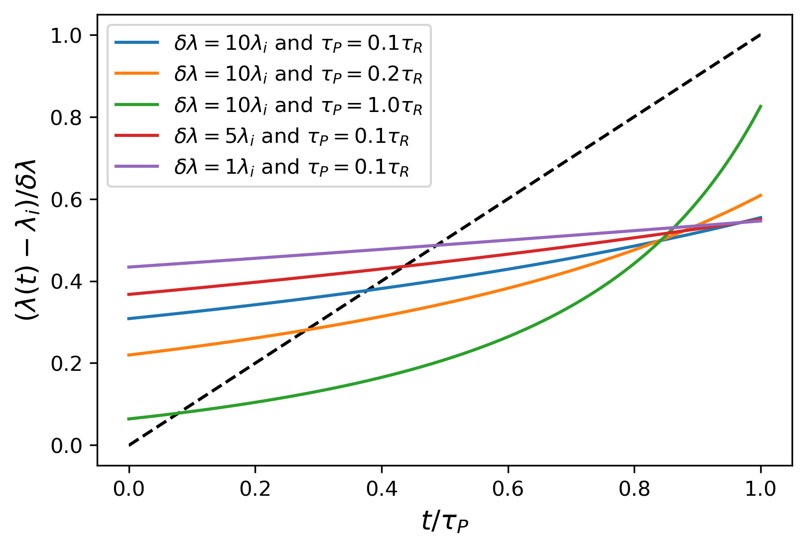
Figure 1: Optimal protocols obtained for the different parameters used in this work. Here, $\delta\lambda=(\lambda_{f}-\lambda_{i})$, the dashed black line represents the linear protocol, $\lambda_{i}=0.3\ \mathrm{pN/\mu m}$, and $\tau_{R}=63\ \mathrm{ms}$.

III Experimental system

The basis of the experimental apparatus, shown in Fig. 2, consists of a dynamically modulated optical tweezers setup thalyta coupled to a high-speed position detector.

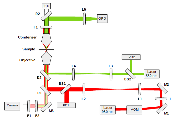
Figure 2: Experimental setup with an infrared laser ($976\ \mathrm{nm}$), a green laser ($532\ \mathrm{nm}$), an acousto-optical modulator (AOM), an objective and a condenser, a quadrant photodetector (QPD), a CCD Camera, an illumination white-LED, photodetectors (PD1-2), mirrors (M1-3), lenses (L1-5), beam splitters (BS1-2), infrared (D1) and green (D2) dichroic mirrors and infrared (F1) and green (F2) filters. Source: ref. thalytaieee .

In our trapping system, a $976\ \mathrm{nm}$ infrared laser Gaussian beam passes through an acousto-optic modulator (AOM) responsible for controlling the position and power note1 of the first order diffraction, which is magnified to fill the entrance of the $100\times$ immersion objective ($\mathrm{NA}=1.3$). In the experiments presented here, only the laser power was modulated by the AOM.

After the objective, a 3D-control nanopositioning stage connected to a sample holder allows the positioning of the sample close to the laser focus. The sample, composed of $2\ \mathrm{\mu m}$ silica beads immersed in purified water, fills a $10\ \mathrm{mm}$ by $20\ \mathrm{\mu m}$ reaction well, sealed with a thin cover glass.

Bright-field imaging, using a CCD camera, locates and monitors the particles in the sample, and to detect their position we use a quadrant photodiode (QPD). An uncollimated $532\ \mathrm{nm}$ probe laser, aligned with the trapping optical path, scatters on the particle, and the outgoing light is collected by a condenser and directed to the QPD. Then, moving the trapped bead over a known distance using the AOM control, it is possible to calibrate the voltage outputs from the QPD into length units and access the particle’s position with a time resolution up to $150\ \mathrm{kHz}$.

In addition, two photodetectors (PDs) monitor the green and infrared laser intensity with the aid of a high-speed multi-function data acquisition (DAQ) board (National Instruments, PCI6259), which is also responsible for controlling the AOM and reading the QPD signals.

A set of lenses is used to change the collimation of the laser beams, and the mirrors direct the light in the desired optical path. Additional red and green dichroic mirrors and filters separate the different wavelengths and prevent camera and QPD saturation.

IV Characterization of the optical potential

When a colloidal particle comes near the focus of the trapping laser, it feels an approximately harmonic potential depending on the system’s parameters, such as the shape and power of the trapping laser, the objective settings, the size and material of the sample, the medium where the particle is immersed, etc. Thus, characterizing the effective optical potential felt by the particle is an essential step for most optical tweezers studies and, mainly for this one, which aims to calculate work, $W$, due to changes in the trap stiffness.

Several methods are available in the literature to calibrate the trap stiffness. Here we use the Power Spectrum Density (PSD), described in jones2015optical , as it is one of the most reliable.

The basic procedure is to trap one particle in the static potential and track its position $x_{j}$ at a fixed sampling frequency $f_{s}$ for a total time $T_{s}$. Here, $x_{j}=x(t_{j})$, where $t_{j}=j\Delta t$ being $j=1,...,N$ and $\Delta t=1/f_{s}$.

Applying a discrete Fourier transform to the trajectory data, one has:

$$\breve{x_{k}}=\Delta t\sum^{N}_{j=1}e^{i2\pi f_{k}t_{j}}x_{j},$$ (8)

where $f_{k}=k/T_{s}$ and $k=-N/2+1,...,N/2$. After that, we can calculate the PSD given by $P_{k}=|\breve{x}_{k}|^{2}/T_{s}$. Following the standard procedure jones2015optical , the data is compressed by blocking note2 .

The final PSD, $\langle P_{k}\rangle$, is equivalent to:

$$\langle P_{k}\rangle=\frac{D/(2\pi^{2})}{f^{2}_{c}+f_{k}},$$ (9)

being $D$ the diffusion coefficient and $f_{c}=\kappa(2\pi\gamma)^{-1}$ the corner frequency, which depends on the trap stiffness ($\kappa$) and the particle friction coefficient ($\gamma$).

Thus, for each set of data, collected at a $10\ \mathrm{kHz}$ acquisition rate and measurement time of $10\ \mathrm{s}$, we obtain the trap stiffness using Eq. 9 (Fig. 3). Repeating this calibration for several laser powers, Fig. 4 was generated. This curve allows us to estimate the potential spring constant directly from the reference infrared PD signal without needing further calibrations.

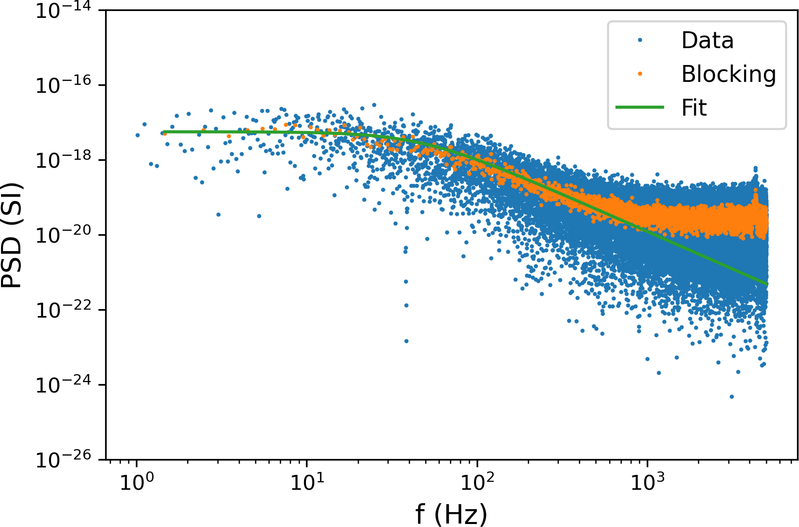
Figure 3: Power Spectrum Density (PSD, in SI units) for a trapped particle.

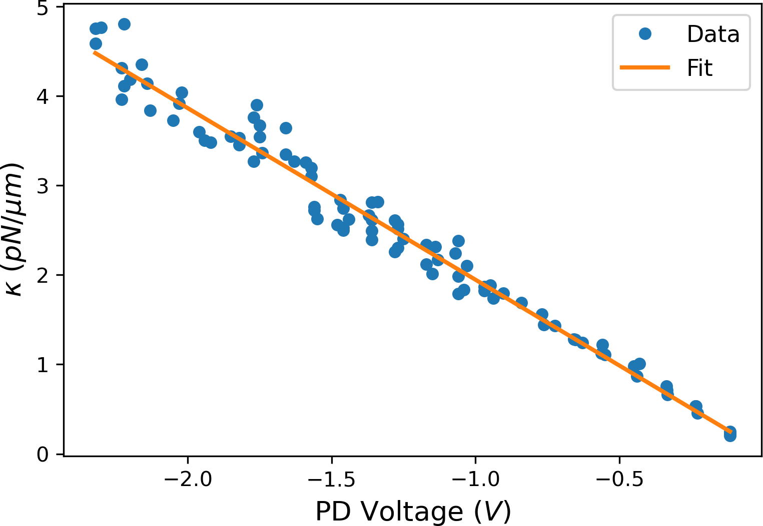
Figure 4: Trap stiffness versus infrared PD voltage (proportional to laser power) at the sample. Fit equation: $y=(-1.92\pm 0.03)x+(0.03\pm 0.04)$.

V Protocols application

The basic procedure to apply the protocols described in Section II is to dynamically control the potential applied to the trapped particle by modulating the laser intensity. Since the particle must be in thermal equilibrium at the beginning of the protocol, during a time interval $\tau_{eq}>\tau_{R}$, being $\tau_{R}=\gamma/\lambda_{i}$ the relaxation time, the laser power is kept at a constant value equivalent to the state $\lambda_{i}$. After that, the desired protocol is applied, finishing at the final trap stiffness equivalent to $\lambda_{f}$.

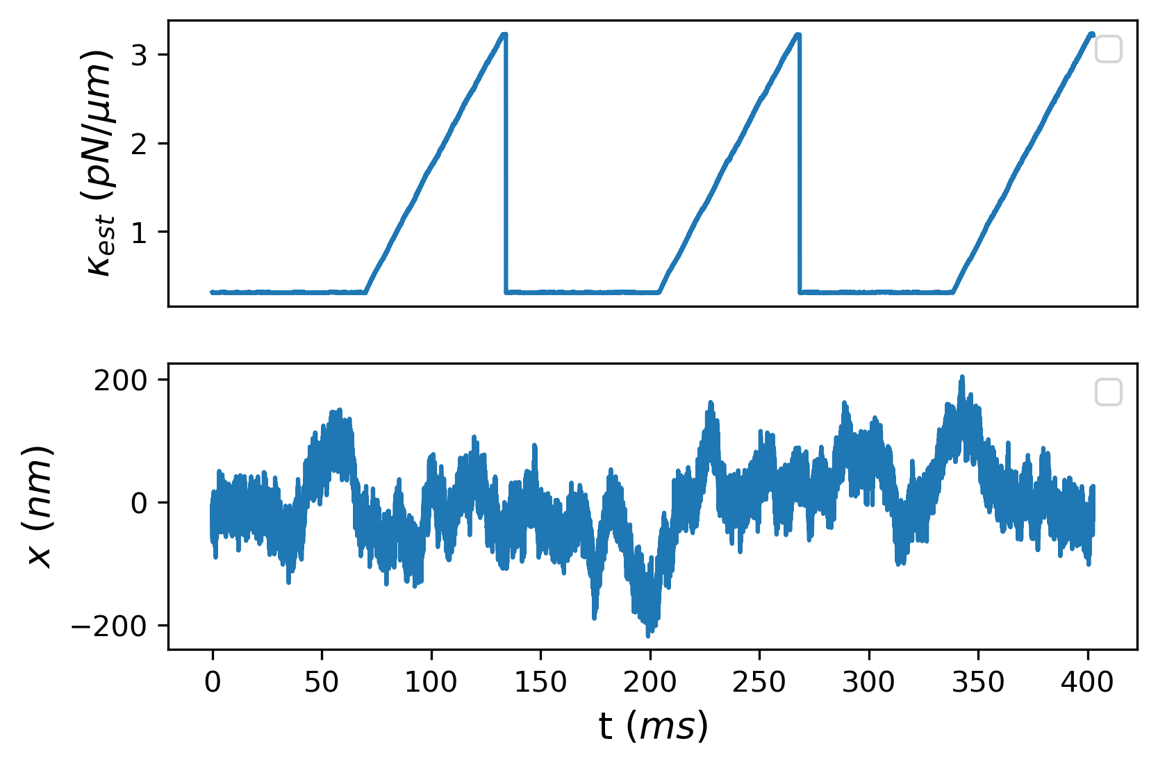
Figure 5: Estimated trap stiffness (top) and particle position (bottom) for three repetitions of a linear protocol with $\tau_{eq}=70\ \mathrm{ms}$, $\lambda_{i}=0.3\ \mathrm{pN}/\mu\mathrm{m}$, $\delta\lambda=10\lambda_{i}$ and $\tau=\tau_{R}=63\ \mathrm{ms}$.

Acquiring the QPD and infrared PD signals simultaneously during the experiment, one has the estimated trap stiffness $\kappa_{est}$ and the particle position $x$, as shown in Fig. 5. Using these data for each cycle, the stochastic work for each trajectory can be directly calculated by discretizing Eq. 3 sekimoto ; gavrilov :

$$W=\Delta t\sum_{n=0}^{N}\frac{d\kappa}{dt}\frac{x^{2}}{2}.$$ (10)

Thus, by repeating the same protocol $n$ times, one can build a histogram of $W$ from all the measurements, as the one shown in Fig. 6. In this present study, the number of repetitions $n$ ranged from 6000–9000 times, and the implementation of the optimal protocol, proposed in ref. seifert , was compared with a linear protocol for each set of parameters. While the linear protocol takes the particle from $\lambda_{i}$ to $\lambda_{f}$ linearly over time, the optimal protocol follows the Eq. 5.

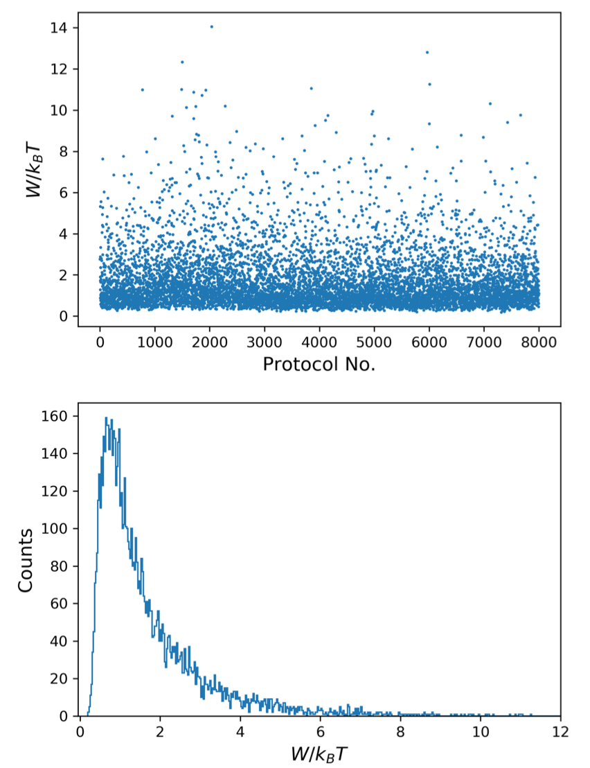
Figure 6: Measured work values calculated for each stochastic trajectory of the linear protocol for $\lambda_{i}=0.3\ pN/\mu m$ and $\delta\lambda=10\lambda_{i}$, with $\tau_{eq}=70\ \mathrm{ms}$ and $\tau=\tau_{R}=63\ \mathrm{ms}$. The top figure shows all the $n=8000$ measurements, while the bottom image shows a histogram with 500 bins.

Keeping fixed $\lambda_{i}=0.3\ \mathrm{pN/\mu m}$, $\tau_{R}=\gamma/\lambda_{i}=63\ \mathrm{ms}$, $\tau_{eq}=70\ \mathrm{ms}$, $T=300\ \mathrm{K}$, and changing the protocol time and amplitude of modulation according to the parameters shown in Fig. 1, it is possible to verify that the optimal protocol indeed has a lower average work than the linear protocol. Moreover, according to Table 1, we can observe that the optimal work is always smaller than the linear one, except for small changes in trap stiffness, which have almost the same work values.

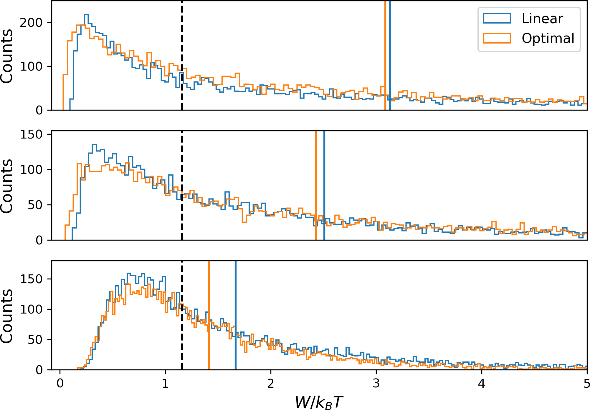
Figure 7: Work histograms for linear and optimal protocols with $\delta\lambda=10\lambda_{i}$ and different protocol times ($\tau=0.1\,\tau_{R}$, $\tau=0.2\,\tau_{R}$ and $\tau=\tau_{R}$, from top to bottom). The free energy difference is represented by the dashed black line and the average work of the linear and optimal protocols by the solid blue and orange lines, respectively. Data collected at $100\ \mathrm{kHz}$ acquisition rate.

Besides, we can also observe the behavior of the work distributions for different protocol times with the same modulation amplitude. As expected by the Clausius inequality clausius , the mean work converges to the free energy difference for longer times, as represented in Fig. 7.

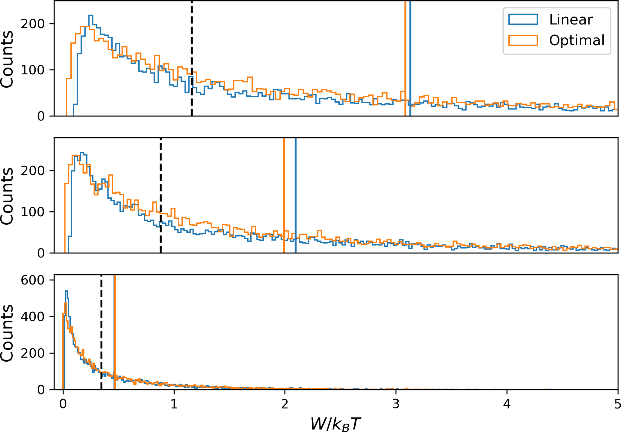
Figure 8: Histograms of work distribution for $\tau=0.1\,\tau_{R}$ and different amplitudes: $\delta\lambda=10\lambda_{i}$, $\delta\lambda=5\lambda_{i}$, and $\delta\lambda=1\lambda_{i}$ (from top to bottom). The black dashed-lines represent the free energy differences, $\Delta F$, while the average work of the linear and optimal protocols are represented by the solid blue and orange lines, respectively.

As an independent sanity check, we used the same collected data for the stochastic trajectories to verify the Jarzynski equality jarzynski :

$$e^{-\Delta F/k_{B}T}=\langle e^{-W/k_{B}T}\rangle,$$ (11)

where $\Delta F$ is the free energy difference given by:

$$\Delta F=F_{f}-F_{i}=-k_{B}T(\log Z_{f}-\log Z_{i})$$ (12)

with $Z_{i}$ and $Z_{f}$ being to the initial and final partition function, respectively. Furthermore, since the Jarzynski relation can be applied to arbitrary nonequilibrium (finite-time) processes, with the only requirement being to start from equilibrium, the right-hand side of Eq. (11) can be calculated directly from our data, being independent of the protocol used. Therefore, we use this fact to verify the self-consistency of our measurements. The results are shown in Table 1.

Table 1: Final results for linear (L) and optimal (O) protocols.

$\delta\lambda/\lambda_{i}$	$e^{-\Delta F/K_{B}T}$	$\tau/\tau_{R}$	Type	$n$	$\left\langle e^{-W/K_{B}T}\right\rangle$	$\left\langle W\right\rangle/K_{B}T$
10	0.30(2)	0.1	L	9000	0.29274(5)	3.1508(2)
			O	9000	0.28870(1)	3.10602(4)
		0.2	L	6000	0.29189(4)	2.5238(1)
			O	6000	0.29139(1)	2.44431(4)
		1	L	8000	0.30108(1)	1.67866(4)
			O	9000	0.32611(6)	1.42051(2)
5	0.41(3)	0.1	L	9000	0.38722(6)	2.1103(1)
			O	9000	0.38753(1)	2.00671(3)
1	0.71(5)	0.1	L	9000	0.70661(2)	0.46802(3)
			O	9000	0.70399(3)	0.470760(4)

VI Conclusions

In conclusion, as summarized in Table 1, these preliminary experimental results show that the average work for the proposed optimal protocols is indeed smaller than linear ones, and the Jarzynski equality is satisfied with good precision for most cases. Our next steps are to better understand and decrease the experimental uncertainties and to verify the moving trap case, which corresponds to the second model studied in ref. seifert , where the equilibrium position of the trap is dynamically controlled. These studies illustrate the great potential of optical tweezers to contribute and to advance the field of nonequilibrium stochastic thermodynamics, which is a broad field of investigation with many applications in physics, chemistry, and biology.

References

- (1) Schmiedl, Tim, and Udo Seifert. ”Optimal finite-time processes in stochastic thermodynamics.” Physical Review Letters 98, 108301 (2007).
- (2) Schmiedl, Tim, et al. ”Optimal protocols for Hamiltonian and Schrödinger dynamics.” Journal of Statistical Mechanics: Theory and Experiment 2009.07 (2009): P07013.
- (3) Gomez-Marin, Alex, Tim Schmiedl, and Udo Seifert. ”Optimal protocols for minimal work processes in underdamped stochastic thermodynamics.” The Journal of chemical physics 129.2 (2008): 024114.
- (4) Bonança, Marcus V.S., and Sebastian Deffner. ”Optimal driving of isothermal processes close to equilibrium.” The Journal of chemical physics 140.24 (2014): 244119.
- (5) Bonança, Marcus V.S., and Sebastian Deffner. ”Minimal dissipation in processes far from equilibrium.” Physical Review E 98.4 (2018): 042103.
- (6) Large, Steven J., and David A. Sivak. ”Optimal discrete control: minimizing dissipation in discretely driven nonequilibrium systems.” Journal of Statistical Mechanics: Theory and Experiment 2019.8 (2019): 083212.
- (7) Kamizaki, Lucas P., Bonança, Marcus V.S. and Muniz, Sérgio R. ”Performance of optimal linear-response processes in driven Brownian motion far from equilibrium”, arXiv:2204.07145 (2022), https://doi.org/10.48550/arxiv.2204.07145.
- (8) Kamizaki, Lucas P., Studies of stochastic thermodynamics with optical tweezers. M.S. thesis, Universidade de São Paulo, 2022. https://doi.org/10.11606/D.76.2022.tde-13072022-121617.
- (9) Otani, Sandro K., Martins, Thalyta T., Muniz, Sérgio R., de Sousa Filho, Paulo C., Sigoli, Fernando A., and Nome, René A. ”Spectroscopic characterization of rare events in colloidal particle stochastic thermodynamics.” Frontiers in Chemistry, 10, 2022.879524 (2022). https://doi.org/10.3389/fchem.2022.879524.
- (10) Martínez, I. A., Roldán, É., Dinis, L., & Rica, R. A. (2017). Colloidal heat engines: a review. Soft matter, 13(1), 22-36.
- (11) Sekimoto, Ken. ”Langevin equation and thermodynamics.” Progress of Theoretical Physics Supplement 130 (1998): 17-27.
- (12) Essentially, the radio-frequency (RF) signal, generated by a voltage-controlled oscillator (VCO) circuit, feeds a piezoelectric coupled to the AOM crystal, which induces the propagation of acoustic waves through the material. When the laser light passes perpendicularly through this wave, a diffraction pattern is created dependent on the amplitude and frequency of the signal. By controlling the amplitude of the RF signal, one can restrict the amount of light diffracted, resulting in control of the beam power. With the aid of a PD, it is possible to calibrate the power of the chosen beam as a function of the applied voltage.
- (13) Martins, Thalyta Tavares, and Muniz, Sérgio R. ”Dynamically controlled double-well optical potential for colloidal particles.” 2021 SBFoton International Optics and Photonics Conference (SBFoton IOPC). IEEE, 2021. https://doi.org/10.1109/SBFotonIOPC50774.2021.9461866
- (14) Martins, Thalyta Tavares. Aprisionamento óptico de micropartículas e desenvolvimento de potenciais ópticos dinâmicos. M.S. thesis, Universidade de São Paulo, 2019. https://doi.org/10.11606/D.76.2019.tde-12092019-141442.
- (15) Jones, Philip, Onofrio Maragó, and Giovanni Volpe. Optical tweezers. Cambridge: Cambridge University Press, 2015.
- (16) Here, we replace a set of data points with a single coordinate given by the block average. One uses to denoted the PSD after blocking procedure.
- (17) Gavrilov, Momčilo. Experiments on the thermodynamics of information processing. Springer, 2017.
- (18) Clausius, Rudolf. ”On the treatment of differential equations which are not directly integrable.” The Mechanical Theory of Heat, with Its Applications to the Steam Engine and to the Physical Properties of Bodies (1867): 1-13.
- (19) Jarzynski, Christopher. ”Nonequilibrium equality for free energy differences.” Physical Review Letters 78.14 (1997): 2690.