SALT3-NIR: Taking the Open-Source Type Ia Supernova Model to Longer Wavelengths for Next-Generation Cosmological Measurements

Abstract

A large fraction of Type Ia supernova (SN Ia) observations over the next decade will be in the near-infrared (NIR), at wavelengths beyond the reach of the current standard light-curve model for SN Ia cosmology, SALT3 ($\sim 2800$–8700 Å central filter wavelength). To harness this new SN Ia sample and reduce future light-curve standardization systematic uncertainties, we train SALT3 at NIR wavelengths (SALT3-NIR) up to 2 $\mu$m with the open-source model-training software SALTshaker, which can easily accommodate future observations. Using simulated data we show that the training process constrains the NIR model to $\sim 2$–3% across the phase range ($-20$ to $50$ days). We find that Hubble residual (HR) scatter is smaller using the NIR alone or optical+NIR compared to optical alone, by up to $\sim 30$% depending on filter choice (95% confidence). There is significant correlation between NIR light-curve stretch measurements and luminosity, with stretch and color corrections often improving HR scatter by up to $\sim 20\%$. For SN Ia observations expected from the Roman Space Telescope, SALT3-NIR increases the amount of usable data in the SALT framework by $\sim 20$% at redshift $z\lesssim 0.4$ and by $\sim 50$% at $z\lesssim 0.15$. The SALT3-NIR model is part of the open-source SNCosmo and SNANA SN Ia cosmology packages.

ʻ ‘

1 Introduction

Future time-domain surveys will discover samples of tens to hundreds of thousands of Type Ia supernovae (SNe Ia), which will be used to measure cosmological parameters such as the Hubble-Lemaître constant (H₀) and the dark energy equation of state (EoS; e.g., Garnavich et al., 1998; Riess et al., 1998; Perlmutter et al., 1999; Scolnic et al., 2018; Brout et al., 2022). For cosmological measurements, SN Ia samples require precise photometric (and often spectroscopic) observations with a relatively high cadence over a series of weeks, and a well-trained model describing the spectral evolution of SNe Ia over time. This model is used for brightness standardization and subsequent luminosity-distance measurements, typically by applying corrections to an observed SN Ia brightness based upon the fitted light-curve shape (here called “stretch") and color (e.g., the Tripp equation; Tripp, 1998). Historically, most SN Ia observations have been at optical wavelengths ($\sim 3000$–8000 Å; e.g., Hamuy et al., 1996; Riess et al., 1999; Astier et al., 2006; Jha et al., 2006, 2007; Holtzman et al., 2008; Hicken et al., 2009; Contreras et al., 2010; Stritzinger et al., 2011; Hicken et al., 2012; Jones et al., 2017; Foley et al., 2018; Abbott et al., 2019), which has led to models of SN Ia spectral energy distributions (SEDs) with similar wavelength coverage (e.g., Guy et al., 2005, 2007, 2010; Betoule et al., 2014; Mosher et al., 2014; Saunders et al., 2018; Leget et al., 2020; Taylor et al., 2021).

There are indications that the remaining scatter in residuals in a Hubble diagram made with optical distance measurements (“intrinsic scatter”; e.g., Scolnic et al., 2018) can be reduced by up to $\sim 60\%$ using rest-frame near-infrared (NIR) SN Ia observations (Elias et al., 1986; Krisciunas et al., 2004a; Mandel et al., 2011; Dhawan et al., 2018; Avelino et al., 2019). Such an improvement would require a large sample of rest-frame NIR SN Ia spectra and photometry, and a well-trained model with coverage at these wavelengths to be used for brightness standardization. While there have been SN Ia light-curve models trained at NIR wavelengths (e.g., Burns et al., 2011, 2014; Mandel et al., 2011, 2020), most large-sample cosmological analyses including SNe Ia for the last decade (Guy et al., 2010; Conley et al., 2011; Betoule et al., 2014; Riess et al., 2018; Sako et al., 2018; Scolnic et al., 2018; Brout et al., 2019; Jones et al., 2019; Brout et al., 2022) have used the SALT2 framework for brightness standardization (Guy et al., 2007, 2010). SALT2 is a principal component analysis (PCA)-like SED time-series model with continuous wavelength coverage (2000–9200 Å), and it is trained on a mix of spectra and photometry from SNe Ia over a wide range in redshift $z$, light-curve stretch, and color. This model is well understood and thoroughly vetted, covers a relatively large phase range, spans slightly beyond optical wavelengths, obviates the need for K-corrections, and has a diverse, open-source training sample. If reliably extended to the NIR, SALT can continue providing a robust open-source model for the future of SN Ia light-curve fitting.

The next decade of SN Ia surveys from space, which in particular includes the Nancy Grace Roman Space Telescope (hereafter Roman), will observe primarily at NIR wavelengths. The natural choice of model to harness this new wealth of data is SALT owing to its consistent use in cosmological analyses (for a summary of other reasons, see Kenworthy et al., 2021, hereafter K21). Although SALT2 has already been extended to NIR wavelengths for simulation studies (Pierel et al., 2018, hereafter P18), the resulting model was not fully trained or validated and is insufficient for cosmological analyses using real data. The SALT3 model from K21 has an improved and open-source training code and sample compared with SALT2, and its wavelength coverage in the red extended from $0.92\,\mu$m to $1.1\,\mu$m (central filter wavelength 8700 Å). However, most low-redshift ($z\lesssim 0.15$) SN Ia observations expected from Roman are beyond the red end of the SALT3 wavelength range and will not currently be used for distance measurements. If this gap is not addressed with a redder rest-frame model, it will be necessary to observe a low-$z$ sample of SNe Ia at optical wavelengths from the ground (e.g., Foley et al., 2018), and combine these with a sample of higher-$z$ SNe Ia whose NIR observations will be probing rest-frame optical wavelengths.

To include the full range of observations expected from Roman in the robust SALT framework, and to enable future cosmological inference at NIR wavelengths, a new version of the model is needed. To address this need, we perform the first robust training of the SALT3 model to $2\,\mu$m using $166$ SNe Ia with rest-frame NIR observations, producing a model that we label as “SALT3-NIR.” While the data volume and calibration are not yet of the same quality as optical data, this training sample will be continuously improved in the future and the model kept up-to-date with the open-source SALTshaker framework. This work enables Roman SN Ia data to be utilized as they become available instead of waiting until there is a sufficient SN Ia sample to train a Roman-only SALT model in the NIR, and produces an improved model for accurate simulations or fitting of early Roman observations. The full training sample used here, as well as the resulting model, will be made public once this manuscript is published.

We begin with a discussion of the SALT3 formalism in Section 2, followed by a description of the NIR training dataset in Section 3 that is used to perform the model training in Section 4 and validation in Section 5. Section 5 also contains an analysis of improvements for NIR cosmology relative to existing models. We conclude in Section 6.

2 The SALT3 Model

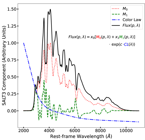
Figure 1: The primary components that make up the existing SALT3 model at peak ($p=0$) brightness (black solid). The $M_{0}$ component (red dotted) defines a “baseline” SN Ia spectrum, the $M_{1}$ component (green dashed) controls the stretch of a given SN, and the color-law (blue dash-dot) is equivalently $A_{\lambda}-A_{B}$. The terms $x_{0}$, $x_{1}$, and $c$ are free fitting parameters.

Here we briefly review the formalism of the SALT3 model; for more details, see K21. SALT3 is based upon the original SALT framework (Guy et al., 2005, 2007), which gives the spectral flux ($F$) as a function of rest-frame phase ($p$) and wavelength ($\lambda$):

$$F(p,\lambda)= x_{0}\left[M_{0}(p,\lambda)+x_{1}M_{1}(p,\lambda)\right]$$

$$\cdot\exp{(c\cdot CL(\lambda))}\,.$$ (1)

The model is described by three components characterizing the population of SNe as determined in the training process, and three parameters characterizing each object in individual light-curve fits. The first two components are $M_{0}(p,\lambda)$, which represents a “standard” SN Ia, and $M_{1}(p,\lambda)$, which contributes a first-order linear correction to the baseline flux. Finally, there is a “color law” component controlling the effects of intrinsic color variation and dust, $CL(\lambda)$. $M_{0}$ and $M_{1}$ are defined as flux surfaces using an interpolated grid in phase and wavelength space that is defined by the training process, while $CL$ is defined as a polynomial (Figure 1). The remaining terms in Equation 2 are the free parameters used to fit SN Ia light-curve data. The parameter $x_{0}$ is the overall flux normalization, $x_{1}$ is the contribution of the $M_{1}$ correction term and is a measure of SN Ia light-curve shape or “stretch,” and $c$ is a measure of SN Ia “color.” These three parameters are used as part of the Tripp (1998) equation to measure the luminosity distance to each SN Ia (e.g., Scolnic et al., 2018).

2.1 SALT Distance Determinations

Accurately measuring SN Ia luminosity distances in the SALT framework is a two-step process. First, best-fit parameters from Equation 2 ($x_{0},x_{1},c$) are measured for a given light curve. These parameters are used to correct the measured apparent magnitude and infer a luminosity distance using the Tripp (1998) equation,

$$\mu=-2.5\,log_{10}(x_{0})+\alpha x_{1}-\beta c-M_{0}\,,$$ (2)

where $\alpha$ $(\beta)$ is the coefficient between luminosity and stretch (color), and $M_{0}$ is the SN Ia absolute magnitude. In this work (Section 5), the $\alpha,\beta,M_{0}$ nuisance parameters are determined by the SALT2mu method described by Marriner et al. (2011). SALT2mu determines the distance moduli separately from the cosmology fit by minimizing the Hubble residuals in redshift bins. This cosmology-independent method allows us to directly compare distances measured by different SALT models without considering the impact of different cosmological assumptions. When comparing SALT3 and SALT3-NIR derived distances in Section 5, we are only concerned with relative differences between the models, and therefore we ignore corrections for host-galaxy mass (e.g., Hamuy et al., 1996; Ivanov et al., 2000; Kelly et al., 2010; Sullivan et al., 2010) and selection bias (Kessler & Scolnic, 2017). These additional corrections are required to measure cosmological parameters (e.g., Scolnic et al., 2018), but are not needed to compare Hubble residuals with different light-curve models.

2.2 SALT2-Extended

While the SALT models have been used for optical cosmological measurements over the last $\sim 15$ yr, there has been only one attempt to extend SALT to NIR wavelengths. P18 used the template from Hsiao et al. (2007), warped to photometry from the Carnegie Supernova Project (CSP), to approximately extend the SALT2 model for use in simulations in advance of future NIR surveys (e.g., Hounsell et al., 2018; Rose et al., 2021). The model (here “SALT2-Extended”), which is not trained on spectra nor a procedure to train possible relationships between the NIR and light-curve parameters $x_{1}$ or $c$, is not suitable for SN Ia cosmological parameter measurements in the NIR. Still, SALT2-Extended serves as a useful baseline for what the components of SALT3 may look like in the NIR, and provides the only data-driven means of simulating NIR photometry with an independent (but similarly conceived) model of SN Ia SED evolution. We therefore make use of SALT2-Extended in simulations for validation purposes in Section 5.

3 SALT3-NIR Training Sample

We review the K21 compilation of training data in Section 3.1, which was used to train the SALT3 model to $\sim 1.1\,\mu$m. We build upon this sample by adding a compilation of NIR photometry and spectra presented in Section 3.2. The NIR compilation includes public data (Section 3.2.1), and a series of new SNe Ia observed in the NIR (Sections 3.2.2- 3.2.4). Using this sample of photometric and spectroscopic data, we train the SALT3 model to a maximum wavelength of 2 $\mu$m in Section 4, resulting in the SALT3-NIR model. The full training sample described here will be released publicly alongside the final model.

3.1 K21 Sample

In K21, the most recent SALT2 training sample from Betoule et al. (2014, the “Joint Light Curve Analysis,” JLA) was augmented with light curves of an additional $\sim 700$ SNe Ia from a combination of the second data release of the Carnegie Supernova Project (CSP; Contreras et al., 2010; Stritzinger et al., 2011; Krisciunas et al., 2017), the fourth data release from the Center for Astrophysics SN Ia program (CfA4; Hicken et al., 2012), as well as the Foundation Supernova Survey (Foley et al., 2018; Dettman et al., 2021), the Pan-STARRS Medium Deep Survey (PS1 MDS; Jones et al., 2017; Villar et al., 2020; Hosseinzadeh et al., 2020), and the Dark Energy Survey (DES; The Dark Energy Survey Collaboration, 2005; Abbott et al., 2019; Brout et al., 2019).

The spectroscopic sample was bolstered by spectra from the KAEPORA database (Siebert et al., 2019), the majority of which originate from the Berkeley SN Ia Program (BSNIP; Silverman et al., 2012; Stahl et al., 2020). Light-curve quality cuts were applied to the K21 sample requiring (in the rest frame, relative to $B$-band time of maximum light) at least four photometric measurements within $-10$ to $+35$ days, at least one measurement between $+5$ and $+20$ days, measurements in two filters between $-8$ and $+20$ days, and at least one measurement within $-10$ to $-1$ days. All photometric data zero-points and filter wavelength shifts were recalibrated using the “Supercal” cross-calibration methodology of Scolnic et al. (2015), which used the $3\pi$ sky coverage of the PS1 photometric system to determine precise offsets between PS1 (which has been measured to $<10$ mmag precision) and other photometric systems.

After all cuts have been applied, the compilation of training data includes 1083 SNe Ia, each with a well-sampled light curve, and 1207 spectra from 380 SNe Ia. We show the density of photometric and spectroscopic data included in this compilation of optical training data in Figure 2. See K21 for a full description of the composition of the sample, as well as characteristics including distributions of redshift, stretch, and color. The only additions to the K21 sample when training the optical portion of SALT3-NIR are the optical companion light curves of new SNe Ia with NIR observations (see next section) and updates to the photometric calibration described by Brout et al. (2021). This effort utilized the public Pan-STARRS stellar photometry catalog (Currie et al., 2020) to cross-calibrate against tertiary standards released by individual SN Ia surveys, and the resulting improvements have already been applied to the SALT3 model released by K21.

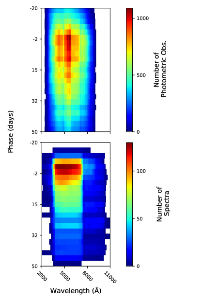
Figure 2: The density of photometric (filter effective wavelength, top) and spectroscopic (bottom) data in the K21 sample, as a function of rest-frame wavelength and days relative to peak brightness (phase).

3.2 Near-Infrared Sample

We have compiled a large sample of SNe Ia with publicly available data in the rest-frame NIR, which come primarily from the CfA and CSP surveys but also other SNe Ia reported in the literature (Section 3.2.1). Additionally, we have made use of the Hubble Space Telescope (HST) observations produced as part of multiple HST programs designed to bolster space-based NIR SN Ia data (Sections 3.2.2-3.2.3), and a large sample of new ground-based NIR light curves described in Section 3.2.4. This work does not produce any updated photometry or spectra, but instead relies upon previous or ongoing efforts to build a NIR SN Ia sample. Accordingly, we have assumed accurate calibration for all the data used here, a caveat discussed more in Section 6. Characteristics of the final training sample are detailed in Section 3.2.5.

3.2.1 Public Data

The compilation of public NIR data includes 107 SNe, each with an optical+NIR light curve (CfA: Wood-Vasey et al. 2008; Hicken et al. 2009; Hicken et al. 2012, Friedman et al. 2015; Marion et al. 2016; CSP: Contreras et al. 2010; Stritzinger et al. 2010; Stritzinger et al. 2011; Krisciunas et al. 2017, and other groups: Krisciunas et al. 2003; Krisciunas et al. 2004b; Krisciunas et al. 2007; Valentini et al. 2003; Stanishev et al. 2007; Pignata et al. 2008; Leloudas et al. 2009). This sample includes 15 NIR spectra of 12 SNe, with large gaps of coverage in rest-frame phase relative to peak that are supplemented in the following sections.

3.2.2 SIRAH

SIRAH was a 2 yr HST program (2020–2021) that concluded in Cycle 28, having observed a new sample of SNe Ia in the Hubble flow ($0.02\lesssim z\lesssim 0.07$) in the NIR with both HST photometry and slitless spectroscopy. The final sample consists of 26 SNe Ia from a redshift range of $0.0024<z<0.07$. The design and implementation of the SIRAH program is described by Jha et al. (in prep.), and the HST observations (and details of the surveys, photometry, and spectra) are presented by Pierel et al. (in prep.). From SIRAH, we include 485 photometric observations in 5 WFC3/IR filters, and 36 contemporaneous NIR spectra from the WFC3/IR grism ($\sim 8000$–17,000 Å) and Keck NIRES ($\sim 10,000$–25,000 Å) instruments. Ground-based optical observations of the SIRAH SNe Ia, which come from the Asteroid Terrestrial-impact Last Alert System (ATLAS; Tonry et al., 2018) and the Zwicky Transient Facility (ZTF; Masci et al., 2019), are also included in the sample to accurately measure the time of peak brightness, light-curve stretch, and color.

3.2.3 RAISIN

The RAISIN program (Jones et al., 2022) was an HST program carried out during Cycles 20 and 23. The goal of RAISIN was to observe a statistically significant sample of cosmologically useful, $z>0.1$ SNe Ia in the rest-frame NIR to measure the dark energy equation-of-state parameter, $w=P/(\rho c^{2})$.

RAISIN followed 46 total SNe Ia from the PS1 MDS and the DES SN surveys, 37 of which were used to measure $w$. 18 SNe include three NIR epochs of data in both the $F125W$ and $F160W$ filters, while the remaining SNe include approximately three NIR epochs of data in only the $F160W$ filter. Details of the surveys and methods for deriving photometry are given by Jones et al. (2022). Here, as with SIRAH, we include the ground-based optical and HST NIR data for those 37 SNe in our training sample.

3.2.4 DEHVILS

The DEHVILS survey (Dark Energy, H₀, and peculiar Velocities using Infrared Light from Supernovae) is a SN Ia follow-up survey on the UKIRT telescope on the summit of Maunakea, Hawai ‘ i (Peterson et al., in prep.). The survey began in March 2020, and has observed more than 100 $z<0.1$ SNe Ia in the $YJH$ filters with a median of $\sim 5$ epochs of observation per SN. SN targets are selected primarily from ATLAS (Tonry et al., 2018) transient discoveries, and SIRAH targets within an accessible declination range were also prioritized. Light curves are generated using photpipe (Rest et al., 2005), with photometric calibration tied to 2MASS (Skrutskie et al., 2006) using the color transformations derived by Hodgkin et al. (2009). DEHVILS also observed several Milky Way Cepheids in its first year, and those observations are published by Konchady et al. (2022). The first-year SN Ia sample will be described by Peterson et al. (in prep.). For the purposes of being included in this training sample, we once again add the optical data available for each DEHVILS SN Ia, which primarily come from ATLAS.

3.2.5 Full Compilation

Characteristics of the full NIR training sample are listed in Table 1, which describes only the SNe Ia with NIR data. The overall coverage in phase and wavelength space can be seen in Figure 4. In total, we have made use of 166 SNe Ia with NIR data to train SALT3-NIR. Each of these SNe has a well-sampled optical light curve, which is used to constrain the time of maximum light, light-curve stretch, and color (Figure 3). We have applied no additional optical cuts on the training sample, beyond those described by K21 and outlined in Section 3.1. For the NIR, we require at least two epochs of photometry in at least one NIR filter (i.e., $YJH$) within the rest-frame phase range of SALT3-NIR ($-20$ to $50$ days). The additional photometric data coverage from the SNe Ia in Sections 3.2.2–3.2.4 is shown in Figure 5, and an example of the added NIR spectra is shown in Section 5.1.

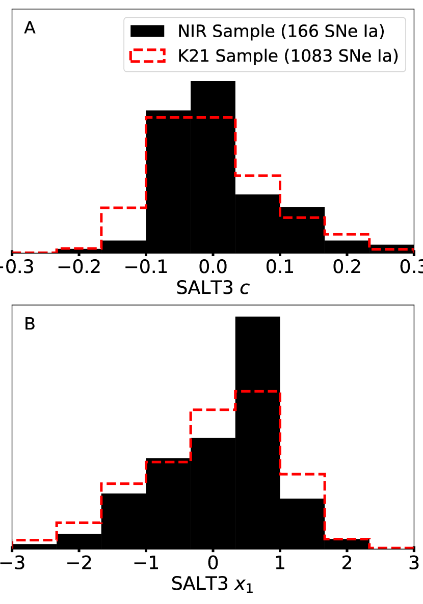
Figure 3: Distributions of SALT3 $c$ (A, top) and $x_{1}$ (B, bottom) for the K21 sample (red dashed line) and the added NIR sample (black).

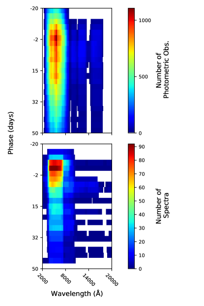
Figure 4: The density of photometric (filter effective wavelength, top) and spectroscopic (bottom) data in the K21+NIR training sample, as a function of rest-frame wavelength and days relative to peak brightness (phase).

Table 1: Full details of the NIR training sample. For information about individual surveys and their references, see Section 3.

Survey	$N_{\rm SN}$	$Y^{a}$	$J^{a}$	$H^{a}$	NIR Spectrab
CfA1	2	0	0	0	2
CfA2	3	0	7	3	1
CfA3	13	140	228	184	5
CfA4p1	2	42	51	58	0
CfA4p2	2	4	24	37	0
CSP	25	572	473	422	1
Foundation	4	0	0	0	4
Other	38	398	838	828	2
Previous Public Total	89	1,156	1,621	1,532	15
DEHVILS	20	183	173	175	0
RAISIN	34	0	57	105	0
SIRAH	23	173	174	83	36
Additional Total	77	356	404	363	36
NIR Training Sample Total	166	1,512	2,025	1,895	51

^aNumber of photometric observations in this rest-frame filter.
^bIncludes spectra with coverage $\lambda\geq 1\,\mu$m.

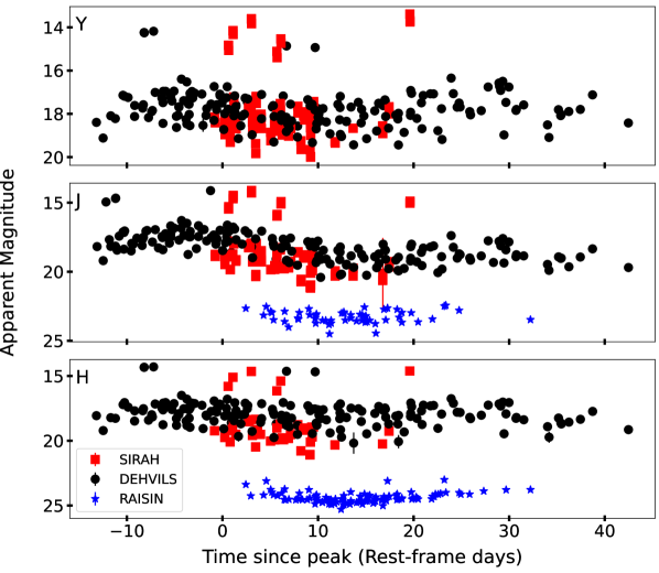
Figure 5: Additional $YJH$ data from the SIRAH, RAISIN, and DEHVILS surveys described in Sections 3.2.2–3.2.4. These light curves are combined with the legacy public NIR data listed in Table 1 to create the full SALT3-NIR training sample.

4 Creating SALT3-NIR with SALTshaker

In an effort to standardize the methodology of training and validating SALT spectrophotometric models, Kenworthy et al. (2021) presented the SALTshaker software program. SALTshaker is a flexible and open-source training and validation pipeline written in Python, which we use here to train the new SALT3-NIR model that extends into the rest-frame NIR. SALTshaker enables the astronomy community to retrain future iterations of SALT3-NIR.

Here we use the same SALTshaker implementation as in K21, with minor changes to accommodate the NIR (see following section). Briefly, the general training procedure builds an empirical SALT3-NIR model by using photometric and spectroscopic data from a SN sample to fit the model parameters with the following methods (see Section 2 of K21).

• The $M_{0}$ and $M_{1}$ principal components are constructed using a second-order B-spline basis, where the values of the knots are determined by fitting the data.

• The SALT3-NIR color law is determined by fitting a fourth-order polynomial with a linear extension.

• The SN Ia parameters $x_{0}$, $x_{1}$, and $c$ are fit simultaneously with the model parameters.

• The SN Ia spectra are recalibrated by using a polynomial (as a function of wavelength) that warps each spectrum to match the SED model. This spectral warping allows the training procedure to account for systematic shifts in the spectral calibration.

• The SALT3-NIR error model is constructed using a zeroth-order B-spline basis, equivalent to binning the data in phase and wavelength.

• The SALT3-NIR color dispersion model uses a single sixth-order polynomial to model the wavelength-dependent scatter simultaneously in each independent filter.

SALTshaker uses an iterative Levenberg-Marquardt algorithm to minimize the $\chi^{2}$ between the model, constructed using the methods above, and the data, while estimating the free parameters of the model. The $\chi^{2}$ includes contributions from the SN photometry and spectra, with additional “regularization" terms that penalize the $\chi^{2}$ for high-frequency $M_{0}$ and $M_{1}$ variations as a function of phase and wavelength, and which ensures the model is separable in phase and wavelength (see K21, Equation 11).

A number of model definitions are used to avoid degeneracies between the model components ($M_{0},M_{1},CL$) and model parameters ($x_{0},x_{1},c$). An example of such a degeneracy is an increase in the value of $x_{0}$ and simultaneous decrease in the amplitudes of $(M_{0},M_{1})$, which would leave the overall model flux unchanged. We add priors that fix the peak $B$-band magnitude to an arbitrary value to avoid an $M_{0}$–$x_{0}$ degeneracy, and that force $(\mu_{x_{1}},\sigma_{x_{1}})=(0,1)$ to avoid an $M_{1}$–$x_{1}$ degeneracy. Another prior forces the final $c$ parameter distribution of the training sample to be 0 ($\mu_{c}=0$), and we anchor the value of the color law at the central wavelengths of the Bessell $B$ and $V$ bands to avoid degeneracies between $c$ and the color law. A final prior reduces the correlation between the $x_{1}$ and $c$ distributions, to avoid confusion of color differences with the $M_{1}$ component. Each of these priors, as well as more details of their purpose, is described in Section 2.1 of K21.

The SALTshaker procedure alternates between fitting the model parameters and fitting the error model, where error-model determination is performed by maximizing the log-likelihood with iMinuit, until the fitting converges. Further details of the SALTshaker training process are given by K21, with their Figure 2 giving an overview schematic of the training procedure. All SALT3 comparisons in Section 5 use this model training process, with the updated calibration discussed at the end of Section 3.1.

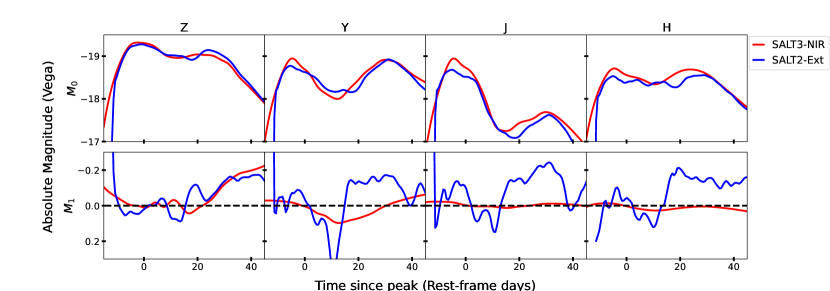
Figure 6: The $M_{0}$ (top row) and $M_{1}$ (bottom row) model components integrated over the $zYJH$ bandpasses. The new SALT3-NIR model is shown in red, while the SALT2-Extended model (previously used for SALT2 simulations in the NIR) is shown in blue.

Figure 7: The SALT3-NIR model flux integrated over optical+NIR bandpasses, as a function of phase and the light-curve stretch parameter, $x_{1}$.

4.1 SALTshaker in the NIR

Extending the wavelength range of SALT3 requires some adjustments to the SALTshaker parameters used by K21. We first extend the $M_{0}$ and $M_{1}$ wavelength ranges to a maximum of 20,000 Å to fully encompass the red edge of all photometric filters and spectra in our sample. Next, while K21 fit the color law polynomial up to 8000 Å and allowed only linear variation in the range 8000–11,000 Å, we use the additional constraining power of NIR data to fit the color-law polynomial up to 12,500 Å. This corresponds to roughly the central $J$-band filter wavelength, and we similarly allow only linear variation in the range 12,500–20,000 Å.

4.2 SALT3-NIR

We train SALT3-NIR using SALTshaker in the manner described in the preceding sections, and with the full training sample from Section 3.2.5. Features of the resulting model are shown in Figures 6–8. In particular, Figure 6 compares SALT3-NIR to SALT2-Extended (Section 2.2). Significant differences are obvious in the smoothness of the model $M_{1}$ component (no regularization was attempted for SALT2-Extended), and while generally the agreement between the two models is quite good, there are significant differences in the $JH$-band peak magnitudes. The impact of these differences on the reference survey simulations for the Roman (Hounsell et al., 2018; Rose et al., 2021) is currently being investigated (Macias et al., in prep.).

Figure 7 shows the model flux integrated over each bandpass for the full optical+NIR range SALT3-NIR, as a function of the light-curve stretch parameter, $x_{1}$. This relation makes the potential of NIR cosmology apparent, as the $JH$ bands have extremely uniform absolute magnitudes and only a weak correlation with light-curve stretch compared to the optical. The sharp variation in the $z$ band around $+20$ days is likely a training artifact, perhaps due to a lack of sufficient coverage in the $x_{1}$ parameter at this phase/wavelength combination. Figure 8 compares the SALT3 and SALT3-NIR color law and color scatter, which describes an intrinsic variance of the SN Ia population unexplained by the model, with significant advancements in the NIR. As we still train the optical portion of the model simultaneously with the NIR, there are differences at bluer wavelengths between SALT3 and SALT3-NIR; these are discussed in Section 6.

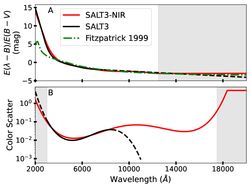
Figure 8: Color law (top) and color scatter (bottom) for SALT3 (black) and SALT3-NIR (red). The dashed region of the SALT3 curve corresponds to the linear regime (color law) or no constraint (color scatter). The same regions are depicted by gray shading for SALT3-NIR. The dust law from Fitzpatrick (1999) (green dash-dot, $R_{V}=3.1$) is shown in the upper panel for comparison.

5 Validating SALT3-NIR

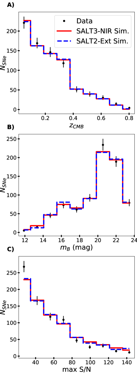
Figure 9: Distributions of redshift (top), SALT2-$m_{B}$ (middle), and maximum S/N (bottom) for training sample data (filled circles), SNANA simulation with SALT3-NIR model (red histogram), and simulation with SALT2-Extended model (blue histogram).

5.1 Producing Simulated Training Samples

To validate the training procedure, we simulate samples of light curves and spectra with observational characteristics [i.e., cadence, signal-to-noise ratio (S/N), and filter/wavelength coverage] matching the training sample described in Section 4. We employ the widely used simulation in the SuperNova ANAlyis (SNANA) software package (Kessler et al., 2009), which generates realizations of SN photometry following Figure 1 of Kessler et al. (2019). Briefly, the simulation begins with a rest-frame “Source SED" and propagates the SN light through an expanding universe, the Milky Way, Earth’s atmosphere, and instrumental filters, finally generating CCD photoelectrons. To produce realistic spectra, the simulation creates Monte Carlo realizations of a source SED using an empirical model of S/N vs. wavelength derived from the training sample described above. These simulations were shown to accurately reproduce both photometry and spectra for the K21 simulated training sample.

The choice of model for simulating light curves and spectra is in principle arbitrary, as SALTshaker is capable of training a model regardless of the underlying simulation framework (Dai et al., in prep.). However, in order to directly use $M_{0}$ and $M_{1}$ recovery precision as a training accuracy metric, it is necessary to select a model described by Equation 2. We therefore make two choices to evaluate the accuracy of our model. First, we use the model produced in Section 4.1 as the source SED, which implicitly assumes that the trained SALT3-NIR model is a perfect description of SNe Ia; this serves as a floor for the validation stage. Second, we produce an identical set of simulations using SALT2-Extended (Section 2.2), which assumes the same formalism as SALT3-NIR but has poorly trained color and stretch relationships as well as a model surface that varies on much smaller wavelength scales compared to SALT3-NIR (see Figure 6 and Pierel et al., 2018). As SALTshaker is designed to ensure a smoothly varying model in phase and wavelength, we expect this scenario to result in a worse training performance. However, this training is a useful exercise as it gives a ceiling for training accuracy, in the case where the frequency of true variability is higher than the level SALTshaker is designed to encode into the final model surface.

As K21 have already confirmed that SALTshaker accurately produces a model given a simulated training sample with realistic SN Ia population parameters, here we check that SALTshaker recovers the underlying NIR model components when training over the updated wavelength range. We therefore produce simulated light curves with the same cadence, filter coverage, number of observations, redshift, and S/N as the true training sample, as well as the same number of spectra with matching wavelength coverage. We do not match the model parameter distributions of $x_{1}$ and $c$ identically to those of the training sample (as K21 did), but instead sample Gaussian distributions that encompass the full range in expected values for these parameters (i.e., $\mu_{x_{1}}=0,\sigma_{x_{1}}=1$ and $\mu_{c}=0,\sigma_{c}=0.1$). The resulting simulation enables us to check if SALTshaker is robust in recovering model surfaces over the entire plausible range in model parameters, given the same volume of data as the training sample in Section 3.2.5.

We create 10 distinct realizations of each simulated training set to ensure sufficient statistical sampling, and Figure 9 displays the agreement of key parameters between randomly selected simulations and the training sample from Section 3. While the simulations are not expected to be a perfect representation of the data, these key distributions of redshift, $m_{B}$, and maximum S/N are all sufficiently well-matched to accept the simulations as appropriate representations of the training sample. An example of observed and simulated NIR spectra is shown in Figure 10.

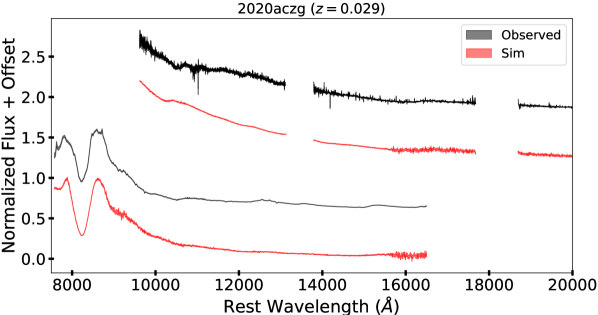
Figure 10: Example of observed (black) and simulated (red) NIR spectra for SIRAH SN 2020aczg. The lower spectra are from the WFC3/IR grism, while the upper are from Keck NIRES. The gaps in the NIRES spectra correspond to atmospheric absorption windows. Every spectrum has a random offset applied to visually distinguish them.

5.2 Training on Simulations with SALTShaker

We train a version of SALT3-NIR on each of the simulated training samples described in Section 5.1. After integrating the simulated and trained $M_{0}$ and $M_{1}$ components over the $YJH$ bandpasses, we compare the recovered model surfaces to those input in the simulation. The SALT3-NIR simulation is an optimistic scenario, in which the training process is perfectly suited to the data. As a result, we find that the $M_{0}$ component is constrained to within $\sim 2\%$ across nearly the full phase range. SALTshaker also recovers the $M_{1}$ component to within $\sim 1\%$ over the same phase range, despite present phase gaps in the NIR training sample (Figure 11). This is due in part to the relatively small $M_{1}$ amplitude compared to the $M_{0}$ component (Figure 6).

On the other hand, the SALT2-Extended simulation is the “pessimistic” scenario, in the sense that its behavior has spurious variability beyond what SALTshaker is attempting to represent. Nevertheless, Figure 12 shows that SALTshaker is still capable of retrieving the $M_{0}$ model component to within $\sim 2$–3% over much of the phase range. The $M_{1}$ component is more poorly retrieved, likely because the high variability in SALT2-Extended is treated as signal by SALTshaker, which is allocated to $M_{1}$. Shown for comparison in Figures 11 and 12 is the recovery of the $B$-band model flux for the same simulation and training processes. Both model components are recovered to within 1% across the full phase range in the optical (apart from $\lesssim-5$ days), setting a fidelity target for the NIR to be reliably used for cosmology.

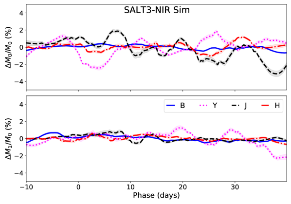
Figure 11: Result of the SALT3-NIR simulation. Difference between the simulated and trained $M_{0}$ (top) and $M_{1}$ (bottom) model components, integrated over the $BYJH$ bandpasses, and divided by the $M_{0}$ component to show fractional differences. Each curve is the average of 10 training sets simulated using SALT3-NIR as the source SED. The $B$ band is shown as a target model fidelity for cosmology.

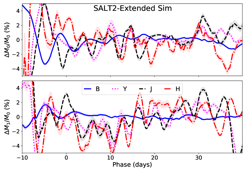
Figure 12: Result of the SALT2-Extended simulation. Difference between the simulated and trained $M_{0}$ (top) and $M_{1}$ (bottom) model components, integrated over the $BYJH$ bandpasses, and divided by the $M_{0}$ component to show fractional differences. Each curve is the average of 10 training sets simulated using SALT2-Extended as the source SED. The $B$ band is shown as a target model fidelity for cosmology.

5.3 Comparison with SALT3

The differences in optical color scatter shown in Figure 8b demonstrate that simultaneously training the optical and NIR slightly degrades the optical model performance. Some variation in scatter is expected, as the model surfaces are continuous in wavelength, but the cause of this degradation is not understood. The most likely culprits are either (a) the NIR is not nearly as well-constrained as the optical owing to a lack of sufficient data, and therefore the NIR scatter impacts optical wavelengths, or (b) the NIR flux is more uniform compared with the optical but SALTshaker is only able to weight individual filters instead of the optical as a whole, which increases the color scatter at optical wavelengths. While the following section suggests that the latter hypothesis is correct, the SALT3 optical-only model should be used in SN Ia cosmology analyses until this optical+NIR scatter issue is understood.

Nevertheless, here we check that optical distances measured with SALT3-NIR are comparable to those of SALT3 by fitting the 10 SALT2-Extended simulated training samples from Section 5.2 with both models, using optical data only and the methods described in Section 2.1. The results are summarized in Tables 2 and 3. The $\alpha$ ($\beta$) parameter shown is the coefficient of relation between SN Ia luminosity and stretch (color), shown in Equation 2. The two models agree within 3$\sigma$ (or $<2$%) for $\beta$, but a significant difference in $\alpha$ ($\sim 20$%) suggests that the NIR training process impacts the overall stretch-luminosity correlation. Since we ignore distance-bias corrections (Section 2.1), the absolute values of $\alpha$ and $\beta$ should not be compared with other studies, but are instead intended for direct comparison between SALT3 and SALT3-NIR. Although there are differences in the measured $\alpha$ and $\beta$ parameters, we find that the slope of the $x_{1}$ ($c$) correlation from measurements with each model is 1.04 (0.99) with a root mean square error (RMSE) of 0.13 (0.02), meaning light-curve parameter measurements are essentially identical for the two models. The Hubble residual root-mean square (RMS) is also not significantly different between the two models.

Table 3 shows that differences in optical distance measurements are $\lesssim 0.01$ mag, meaning that SALT3-NIR is reliable for optical+NIR light-curve fitting or simulations. Here $\Delta\mu$ is the binned residual between measured distances for every simulated SN Ia, and in both tables the uncertainties are the standard error on the mean (SEM) calculated from the 10 simulated training sets.

Table 2: $\alpha,\ \beta$, and Hubble residual RMS measured using SALT3 and SALT3-NIR, and the 10 training sets simulated with SALT2-Extended.

Parameter	SALT3	SALT3-NIR
$\alpha$	0.133$\pm$0.003	0.105$\pm$0.003
$\beta$	2.846$\pm$0.017	2.888$\pm$0.017
HRRMS (mag)	0.117$\pm$0.002	0.118$\pm$0.002

Table 3: Binned differences in optical distance measurements between SALT3 and SALT3-NIR.

$z$ bin	$\Delta\mu$	NSN
	(mag)
0.015–0.026	$0.004\pm 0.001$	78
0.026–0.047	$0.002\pm 0.001$	78
0.047–0.082	$0.000\pm 0.001$	61
0.082–0.146	$0.001\pm 0.001$	80
0.146–0.257	$0.000\pm 0.001$	235
0.257–0.453	$0.005\pm 0.001$	265
0.453–0.800	$0.000\pm 0.001$	125

5.4 Hubble Residuals

Finally, we examine the impact of the NIR in accurately standardizing SNe Ia. First, we take the subset of 105 SNe Ia in our training sample (Section 3) that have sufficient rest-frame $YJH$ data for light-curve fitting without optical bands (i.e., at least 3 data points in at least 1 NIR filter), and are at a sufficiently high redshift such that the effects of peculiar velocities are mitigated (i.e., $z>0.015$). We fit the optical ($BVRI$) light curves in this sample with SALT3, and subsequently fix these time of peak estimates for NIR-only fitting. We reject SNe Ia with optically-fitted parameters $|c|>0.3$ or $|x_{1}|>3$ (e.g., Scolnic et al., 2018). SALT3 and SALT3-NIR distance measurements are derived following Section 2.1. In all cases below the results shown for SALT3 are using only optical fitting and the full set of SALT3 parameters, resulting in RMS values of 0.16–0.19 mag.

In addition to optical SALT3 constraints, we compare SALT3-NIR distance measurements to distances determined using the “SNooPy” ebv_model(2) (Burns et al., 2011, 2014; Avelino et al., 2019; Jones et al., 2022). SNooPy has been effectively the only SN Ia light-curve model capable of reliably fitting the NIR for much of the last decade, and was trained on well-calibrated CSP light curves (Burns et al., 2011; Krisciunas et al., 2017). The more recent BayeSN model (Mandel et al., 2020) also extends to the NIR and uses a different light-curve fitting algorithm. However, the fitting code is not currently open source, and we therefore restrict our comparison to SNooPy.

We split the NIR sample using all combinations of rest-frame NIR filters ($Y$, $J$, $H$, $YJ$, $YH$, $JH$, $YJH$), and fit each subsample with both SALT3-NIR and SNooPy. For each case, we fit with only the light-curve amplitude (i.e., $x_{0}$ for SALT3-NIR and luminosity distance for SNooPy), and separately fit the amplitude with model stretch ($x_{1},s_{BV}$). For subsamples with 2 or more NIR filters, we attempt to include a color parameter ($c,E(B-V)$). We fit with relaxed bounds of $|c|<1,|x_{1}|<4$ for SALT3-NIR and $|E(B-V)|<1.3$ mag, $0.7<s_{BV}<1.3$ for SNooPy (with $R_{V}=1.518$; Burns et al., 2014).

Table 4 shows the results of this fitting process. The SALT3 RMS values correspond to the optical RMS for the respective subsample, while the SALT3-NIR and SNooPy RMS values are the result of fits to the subsample using the given set of parameters. Both SALT3-NIR and SNooPy use flat priors for all parameters, and in cases where stretch (color) is not fit we fix the value to $x_{1}=0$ ($c=0$) for SALT3-NIR and $s_{BV}=0.9$ ($E(B-V)=0$ mag) for SNooPy. This choice is based on Jones et al. (2022), who also found that shifting the fixed parameter value had a negligible impact on Hubble residual RMS. Figure 13 shows the optical+NIR case, while the scenario with the best SALT3-NIR RMS is shown in Figure 14. We cannot fit the optical+$YJH$ case with SNooPy, as the optical data for a large number of the SNe Ia in this sample come from ATLAS, whose wide bandpasses cause known issues with the K-corrections necessary for SNooPy fitting.

The numbers in each Table 4 section correspond to results for the SNe Ia passing cuts for all subsamples in that section. For example, in the first section there are 44 SNe Ia that pass all of the $Y$, $J$, and $H$ amplitude-only fitting procedures, and the RMS values shown (i.e., $\rm{RMS}_{Y}=0.136,\rm{RMS}_{J}=0.161,\rm{RMS}_{H}=0.145$ mag for SALT3-NIR) are based on those identical 44 SNe Ia. This procedure enables a direct comparison between results in a given section, but significantly reduces the sample size in each row. For each amplitude-only fitting procedure, where far fewer fits fail, we show the RMS for all SNe Ia passing that single fit in parentheses. For example while only 26 SNe Ia pass all 4 fitting procedures in the $YJ$ section, 54 SNe Ia are successfully fit when floating only the amplitude. In this scenario, SNooPy produced the lowest RMS while fitting the amplitude only for the sample of 26 SNe Ia, but SALT3-NIR performs the best on the full sample of 54 SNe Ia with sufficient $YJ$ data.

Table 4: Hubble residual RMS comparison between SALT3-NIR, SNooPy, and SALT3.

		Hubble Residual RMS for:
Filters	Parameters	SALT3-NIR	SNooPy	SALT3a	$N_{\rm{SN}}^{b}$
		mag (mag)	mag (mag)	mag (mag)
$Y$	Amplitudec	0.164 (0.151)d	0.190 (0.183)	0.174 (0.135)	31 (74)
$J$	Amplitude	0.169 (0.178)	0.187 (0.207)	0.174 (0.134)	31 (47)
$H$	Amplitude	0.161 (0.158)	0.159 (0.156)	0.174 (0.163)	31 (38)
$Y$	Amplitude, Stretche	0.142	0.172	0.158	28
$J$	Amplitude, Stretch	0.170	0.187	0.158	28
$H$	Amplitude, Stretch	0.135	0.122	0.158	28
$YJ$	Amplitude	0.117g (0.154)	0.111 (0.199)	0.160 (0.136)	21 (46)
$YJ$	Amplitude, Colorf	0.108	0.240	0.160	21
$YJ$	Amplitude, Stretch	0.115	0.116	0.160	21
$YJ$	Amplitude, Stretch, Color	0.118	0.274	0.160	21
$YH$	Amplitude	0.151 (0.160)	0.143 (0.160)	0.160 (0.152)	32 (39)
$YH$	Amplitude, Color	0.149	0.175	0.160	32
$YH$	Amplitude, Stretch	0.151	0.151	0.160	32
$YH$	Amplitude, Stretch, Color	0.153	0.194	0.160	32
$JH$	Amplitude	0.138 (0.159)	0.141 (0.155)	0.117 (0.160)	21 (38)
$JH$	Amplitude, Color	0.116	0.151	0.117	21
$JH$	Amplitude, Stretch	0.158	0.109	0.117	21
$JH$	Amplitude, Stretch, Color	0.129	0.160	0.117	21
$YJH$	Amplitude	0.128 (0.157)	0.116 (0.183)	0.169 (0.162)	24 (37)
$YJH$	Amplitude, Color	0.126	0.184	0.169	24
$YJH$	Amplitude, Stretch	0.126	0.108	0.169	24
$YJH$	Amplitude, Stretch, Color	0.131	0.181	0.169	24
$OPT+YJH$	Amplitude, Stretch, Color	0.116	–	0.169	24

^aCalculated using optical fits (with all SALT3 parameters) to the respective subsample.

^bRefers to the number of SNe Ia that have the rest-frame filters listed and pass fitting cuts.

^cCorresponds to the $x_{0}$ parameter for SALT3-NIR and luminosity distance for SNooPy.

^dNumbers in parentheses correspond to the results for all SNe passing the amplitude-only fitting in that row.

^eCorresponds to the $x_{1}$ parameter for SALT3-NIR and $s_{BV}$ for SNooPy.

^fCorresponds to the $c$ parameter for SALT3-NIR and $E(B-V)$ for SNooPy.

^gBold numbers correspond to cases where the SALT3-NIR RMS is lower than SALT3 with $>95$% confidence

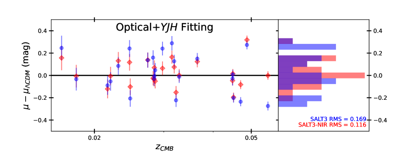
Figure 13: Hubble residuals (with respect to $\Lambda$CDM) when fitting optical+NIR filters with SALT3-NIR (red diamonds), and optical filters with SALT3 from K21 (blue circles). Here, all model parameters are allowed to float.

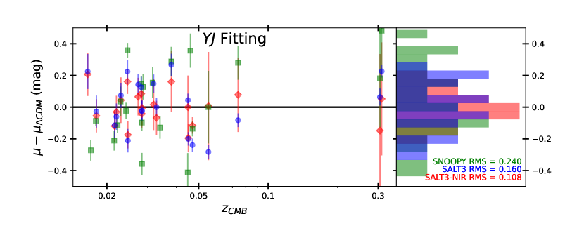
Figure 14: Hubble residuals (with respect to $\Lambda$CDM) when fitting only rest-frame $YJ$ filters with SALT3-NIR (red diamonds) and SNooPy (green squares), and optical filters with SALT3 from K21 (blue circles). Here, the stretch parameter is not allowed to float for SALT3-NIR and SNooPy.

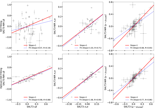
Figure 15: Correlations (black points with error bars) between SALT3 and SALT3-NIR measured values of $c$ (left), $x_{1}$ (center), and $\mu-\mu_{\Lambda\rm{CDM}}$ (right) for $YJH$ (top row) and Optical$+YJH$ (bottom row) fitting scenarios. The SALT3 fits are for the same SNe Ia fit by SALT3-NIR, but using only optical data. Best-fit linear regressions are shown as blue dotted lines, and a slope of 1 (red solid line) is given for comparison.

The SALT3-NIR RMS is lower than SNooPy in 20 of 29 scenarios, and only one scenario is more than 10% higher. Optical distances with SALT3 only produce the lowest RMS in 4 of the 29 scenarios, with the largest difference being the $JH$-band fitting (10–$30$%). In the best SALT3-NIR case ($YJ$, fitting the amplitude and color parameters), we see a $\sim 30$% reduction in residual RMS compared to optical fitting, with a similar effect seen when fitting optical and NIR data simultaneously. Although the sample here is small, we attempt to characterize the significance of this result by bootstrapping the NIR-only sample. We define a new set of parameters $\Delta\mu_{i}$, such that

$$\Delta\mu_{i}=\delta\mu_{i,\rm{NIR}}^{2}-\delta\mu_{i,\rm{Optical}}^{2},$$ (3)

where $\delta\mu_{i}$ refers to the Hubble residual for the $i^{th}$ SN Ia. We bootstrap the set of $\Delta\mu_{i}$ values for every row in Table 4 with 10,000 samples, and find that fitting the NIR data alone provides a lower RMS than optical fitting in 8 scenarios with 95% confidence. We also find that optical+NIR fitting produces a lower RMS than optical-only fitting with 95% confidence. This is in agreement with Avelino et al. (2019), who found that using the NIR, alone or with optical data, resulted in a significant improvement in Hubble residual RMS. However, this is the first attempt at applying stretch and/or color corrections at NIR wavelengths, with these initial results suggesting that stretch corrections at least are certainly worthwhile in the current framework. All scenarios in which the bootstrapping analysis confirmed the SALT3-NIR RMS is lower than SALT3 with $>95$% confidence are bold in Table 4.

Figure 15 shows correlations between SALT3 and SALT3-NIR for measured values of $c,x_{1}$, and $\mu-\mu_{\Lambda\rm{CDM}}$ for the $YJH$ and Optical$+YJH$ fitting scenarios described above. Values measured by SALT3 are still using optical data only, for the same SNe Ia fit by SALT3-NIR. As expected, when optical data are included in SALT3-NIR fitting, the correlation between SALT3 and SALT3-NIR for each parameter is quite strong, with a slope close to 1 for both $c$ (0.98) and $x_{1}$ (1.08). Interestingly, there is still a strong correlation between measurements of $x_{1}$ when optical data are excluded from the SALT3-NIR fit (slope = 1.03, $R=0.71$), though this relationship should be investigated further as it appears driven by a relatively small number of points. Nevertheless, this suggests that the relationship between light-curve stretch and luminosity impacts the NIR as well as the optical, and that the NIR is capable of measuring this relationship on its own. This is supported by consistent improvements in Hubble residual RMS when a stretch parameter is included in NIR-only fitting, shown in Table 4. On the other hand, attempts to measure the $c$ parameter using the NIR alone display very little correlation with optical measurements. This is likely due to the inherent difficulty in measuring color variation in the NIR (e.g., a difference of $\Delta c$ = 0.1 changes the $J-H$ color by 0.003 mag and the $B-V$ color by 0.1 mag), but future work should investigate the possibility that this result could be hinting at a different physical origin for NIR color variation compared to optical. We find that in cases where the difference between optical and NIR measurements of $c$ are large, there is a correspondingly large and opposite difference in measurements of $x_{1}$ that lead to a relatively small change in distance.

6 Conclusion

We have used the open-source Python package SALTshaker to extend the training of SALT3 to $2\,\mu$m. The training sample has been left unchanged in the optical, apart from optical counterparts to the new NIR sample, so that SALT3-NIR is reliable across its full wavelength range, with only slightly higher color scatter in the optical. Future efforts to improve the calibration in the additional training sample, at both optical and NIR wavelengths, would increase the fidelity of the model. Using simulated training samples, we have shown that SALT3 and SALT3-NIR optical distances differ by $<0.01$ mag, and that SALTshaker is able to constrain the source SED to within $\sim 2$–3% in the NIR given our data density, though $\lesssim 1\%$ is the target for a robust cosmological light-curve fitter.

Still, with a sample of low-$z$ SNe having rest-frame NIR photometry, we find that using SALT3-NIR produces comparable single-filter distance measurements relative to the SNooPy light-curve fitter (but improved in $Y,J$). When adding multiple filters or fitting stretch and/or color parameters, SALT3-NIR provided NIR-only Hubble residual RMS values $\sim 0.02$-0.03 mag lower than SNooPy, reaching $<0.11$ mag, which is a $\sim 30\%$ improvement over SALT3 using optical filters for the same SNe Ia. We also find that Hubble residual scatter is lower when using SALT3-NIR and only NIR data than optical distances in 90% of our fitting scenarios (8 scenarios at $>95$% confidence), and that the RMS from optical+NIR light-curve fitting is also lower than optical alone with 95% confidence. These results are in agreement with those of Avelino et al. (2019), who used an amplitude-only fitting procedure, but we find that stretch and color corrections provide a $\sim 10\%$ improvement when fitting $JH$ filters and can result in a similar RMS compared with optical+NIR fitting. Overall, we find that NIR and optical stretch measurements correlate well while color measurements are uncorrelated, though both luminosity corrections often improve NIR distance measurements (by up to $\sim 20\%$ for $JH$ filters with a color correction). More work must be done to understand if the difference between optical and NIR color variation has a physical origin, or simply requires innovations in the modeling or training process to fully harness.

The indication that the NIR alone can provide a lower RMS than optical+NIR, and the large difference in $\alpha$ seen when fitting optical light curves with both SALT3 and SALT3-NIR, suggest that future work should investigate whether adding a new model component to SALT specifically for the NIR would improve distance measurements. The lack of correlation between color measured with optical and NIR filters is likely another indicator of this need. Mandel et al. (2022) found that optical and NIR bands were relatively uncorrelated, which could be providing similar evidence for this result. Simply allowing uncertainties in color scatter to be correlated could be sufficient, and so this concept should also be explored. Significantly more data would be necessary for this investigation, but it should be possible using Roman.

The new wavelength range of SALT3-NIR will enable the analysis of significantly more SN Ia data with Roman, all at $z\lesssim 1$ in the rest-frame NIR where SNe Ia have been shown repeatedly to be better standard candles (e.g., Mandel et al., 2011; Dhawan et al., 2018; Avelino et al., 2019, and see Section 5.4). Using the reference High-latitude Time Domain Survey (HLTDS) from Rose et al. (2021), Figure 16 shows the cumulative fraction of all Roman HLTDS observations usable with SALT3 and SALT3-NIR. At $z\gtrsim 1$ the models are equivalent, as the Roman filters probe the rest-frame optical, but at $z\lesssim 0.5$ in particular SALT3-NIR will be able to fit $\sim 20\%$ more data than SALT3, increasing to $\gtrsim 85\%$ at $z\lesssim 0.1$. Harnessing these lower-$z$ SNe Ia will be particularly valuable for constraints on time-varying dark energy, as they have greater constraining power than other probes at these redshifts (e.g., Jassal et al., 2005; Sendra & Lazkoz, 2012).

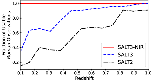
Figure 16: The fraction of all Roman HLTDS observations that SALT2 (black dash-dot), SALT3 (blue dashed), and SALT3-NIR (red solid) are capable of fitting (i.e., the wavelength range fully encompasses the respective filter) as a function of redshift. The difference is most significant at low redshifts, where Roman filters probe the rest-frame NIR.

The SALTshaker training process is flexible, and will easily accommodate new NIR data in the future to continually refine the SALT3-NIR model as more data become available. Roman in particular will provide a wealth of high-precision rest-frame NIR data, including hundreds or thousands of spectra (Rose et al., 2021), which will drastically improve the SALT3-NIR training. While a Roman-only NIR training sample for SALT is plausible in the future, the work herein is necessary now as a robust NIR training methodology, to enable more accurate survey optimization, and produce early-mission SN Ia photometric classification. In advance of Roman there are also a number of ground-based NIR surveys with recent or upcoming public data releases that will be added to the training sample (e.g., Johansson et al., 2021, Hsiao et al., Peterson et al., and Rubin et al. in prep.). Training SALT3-NIR in the SALTshaker framework enables rigorous tests of potential systematic uncertainties arising from the training sample itself, which will be critical as new NIR data are created from future observatories (e.g., Dai et al. and Jones et al., in preparation).

The next decade of SN Ia cosmology is expected to bring a new barrage of data in the NIR, which we are now prepared to harness for improved SN Ia light-curve standardization. SALT3-NIR currently provides the only SED-based, open-source means of simulating, classifying, and analyzing these new SNe Ia in coming years.

References

- Abbott et al. (2019) Abbott, T. M. C., Allam, S., Andersen, P., et al. 2019, ApJ, 872, L30, doi: 10.3847/2041-8213/ab04fa
- Astier et al. (2006) Astier, P., Guy, J., Regnault, N., et al. 2006, A&A, 447, 31, doi: 10.1051/0004-6361:20054185
- Avelino et al. (2019) Avelino, A., Friedman, A. S., Mandel, K. S., et al. 2019, ApJ, 887, 106, doi: 10.3847/1538-4357/ab2a16
- Betoule et al. (2014) Betoule, M., Kessler, R., Guy, J., et al. 2014, A&A, 568, A22, doi: 10.1051/0004-6361/201423413
- Brout et al. (2019) Brout, D., Scolnic, D., Kessler, R., et al. 2019, ApJ, 874, 150, doi: 10.3847/1538-4357/ab08a0
- Brout et al. (2021) Brout, D., Taylor, G., Scolnic, D., et al. 2021, arXiv e-prints, arXiv:2112.03864
- Brout et al. (2022) Brout, D., Scolnic, D., Popovic, B., et al. 2022, arXiv e-prints, arXiv:2202.04077
- Burns et al. (2011) Burns, C. R., Stritzinger, M., Phillips, M. M., et al. 2011, The Astronomical Journal, 141, 19, doi: 10.1088/0004-6256/141/1/19
- Burns et al. (2014) —. 2014, ApJ, 789, 32, doi: 10.1088/0004-637X/789/1/32
- Conley et al. (2011) Conley, A., Guy, J., Sullivan, M., et al. 2011, ApJ Supplement Series, 192, 1, doi: 10.1088/0067-0049/192/1/1
- Contreras et al. (2010) Contreras, C., Hamuy, M., Phillips, M. M., et al. 2010, AJ, 139, 519, doi: 10.1088/0004-6256/139/2/519
- Currie et al. (2020) Currie, M., Rubin, D., Aldering, G., et al. 2020, arXiv e-prints, arXiv:2007.02458
- Dettman et al. (2021) Dettman, K. G., Jha, S. W., Dai, M., et al. 2021, arXiv:2102.06524
- Dhawan et al. (2018) Dhawan, S., Jha, S. W., & Leibundgut, B. 2018, A&A, 609, A72, doi: 10.1051/0004-6361/201731501
- Elias et al. (1986) Elias, J. H., Matthews, K., Neugebauer, G., & Soifer, B. T. 1986, Bulletin of the American Astronomical Society, 18, 1016
- Fitzpatrick (1999) Fitzpatrick, E. 1999, PASP, 111, 63, doi: 10.1086/316293
- Foley et al. (2018) Foley, R. J., Scolnic, D., Rest, A., et al. 2018, MNRAS, 475, 193, doi: 10.1093/mnras/stx3136
- Friedman et al. (2015) Friedman, A. S., Wood-Vasey, W. M., Marion, G. H., et al. 2015, ApJS, 220, 9, doi: 10.1088/0067-0049/220/1/9
- Garnavich et al. (1998) Garnavich, P. M., Jha, S., Challis, P., et al. 1998, ApJ, 509, 74, doi: 10.1086/306495
- Guy et al. (2005) Guy, J., Astier, P., Nobili, S., Regnault, N., & Pain, R. 2005, A&A, 443, 781, doi: 10.1051/0004-6361:20053025
- Guy et al. (2007) Guy, J., Astier, P., Baumont, S., et al. 2007, A&A, 466, 11, doi: 10.1051/0004-6361:20066930
- Guy et al. (2010) Guy, J., Sullivan, M., Conley, A., et al. 2010, A&A, 523, A7, doi: 10.1051/0004-6361/201014468
- Hamuy et al. (1996) Hamuy, M., Phillips, M. M., Suntzeff, N. B., et al. 1996, The Astronomical Journal, 112, 2398, doi: 10.1086/118191
- Hicken et al. (2009) Hicken, M., Wood-Vasey, W. M., Blondin, S., et al. 2009, ApJ, 700, 1097, doi: 10.1088/0004-637X/700/2/1097
- Hicken et al. (2012) Hicken, M., Challis, P., Kirshner, R. P., et al. 2012, ApJS, 200, 12, doi: 10.1088/0067-0049/200/2/12
- Hodgkin et al. (2009) Hodgkin, S. T., Irwin, M. J., Hewett, P. C., & Warren, S. J. 2009, MNRAS, 394, 675, doi: 10.1111/j.1365-2966.2008.14387.x
- Holtzman et al. (2008) Holtzman, J. A., Marriner, J., Kessler, R., et al. 2008, The Astronomical Journal, 136, 2306, doi: 10.1088/0004-6256/136/6/2306
- Hosseinzadeh et al. (2020) Hosseinzadeh, G., Dauphin, F., Villar, V. A., et al. 2020, ApJ, 905, 93, doi: 10.3847/1538-4357/abc42b
- Hounsell et al. (2018) Hounsell, R., Scolnic, D., Foley, R. J., et al. 2018, ApJ, 867, 23, doi: 10.3847/1538-4357/aac08b
- Hsiao et al. (2007) Hsiao, E. Y., Conley, A., Howell, D. A., et al. 2007, ApJ, 663, 1187, doi: 10.1086/518232
- Ivanov et al. (2000) Ivanov, V. D., Hamuy, M., & Pinto, P. A. 2000, ApJ, 542, 588, doi: 10.1086/317060
- Jassal et al. (2005) Jassal, H. K., Bagla, J. S., & Padmanabhan, T. 2005, MNRAS, 356, L11, doi: 10.1111/j.1745-3933.2005.08577.x
- Jha et al. (2007) Jha, S., Riess, A. G., & Kirshner, R. P. 2007, ApJ, 659, 122, doi: 10.1086/512054
- Jha et al. (2006) Jha, S., Kirshner, R. P., Challis, P., et al. 2006, AJ, 131, 527, doi: 10.1086/497989
- Johansson et al. (2021) Johansson, J., Cenko, S. B., Fox, O. D., et al. 2021, ApJ, 923, 237, doi: 10.3847/1538-4357/ac2f9e
- Jones et al. (2017) Jones, D. O., Scolnic, D. M., Riess, A. G., et al. 2017, ApJ, 843, 6, doi: 10.3847/1538-4357/aa767b
- Jones et al. (2019) Jones, D. O., Scolnic, D. M., Foley, R. J., et al. 2019, ApJ, 881, 19, doi: 10.3847/1538-4357/ab2bec
- Jones et al. (2022) Jones, D. O., Mandel, K. S., Kirshner, R. P., et al. 2022, arXiv e-prints, arXiv:2201.07801
- Kelly et al. (2010) Kelly, P. L., Hicken, M., Burke, D. L., Mandel, K. S., & Kirshner, R. P. 2010, ApJ, 715, 743, doi: 10.1088/0004-637X/715/2/743
- Kenworthy et al. (2021) Kenworthy, W. D., Jones, D. O., Dai, M., et al. 2021, arXiv e-prints, arXiv:2104.07795
- Kessler & Scolnic (2017) Kessler, R., & Scolnic, D. 2017, ApJ, 836, 56, doi: 10.3847/1538-4357/836/1/56
- Kessler et al. (2009) Kessler, R., Bernstein, J. P., Cinabro, D., et al. 2009, PASP, 121, 1028, doi: 10.1086/605984
- Kessler et al. (2019) Kessler, R., Brout, D., D’Andrea, C. B., et al. 2019, MNRAS, 485, 1171, doi: 10.1093/mnras/stz463
- Konchady et al. (2022) Konchady, T., Oelkers, R. J., Jones, D. O., et al. 2022, ApJS, 258, 24, doi: 10.3847/1538-4365/ac41d3
- Krisciunas et al. (2004a) Krisciunas, K., Phillips, M. M., & Suntzeff, N. B. 2004a, ApJ, 602, L81, doi: 10.1086/382731
- Krisciunas et al. (2003) Krisciunas, K., Suntzeff, N. B., Candia, P., et al. 2003, AJ, 125, 166, doi: 10.1086/345571
- Krisciunas et al. (2004b) Krisciunas, K., Suntzeff, N. B., Phillips, M. M., et al. 2004b, AJ, 128, 3034, doi: 10.1086/425629
- Krisciunas et al. (2007) Krisciunas, K., Garnavich, P. M., Stanishev, V., et al. 2007, AJ, 133, 58, doi: 10.1086/509126
- Krisciunas et al. (2017) Krisciunas, K., Contreras, C., Burns, C. R., et al. 2017, AJ, 154, 211, doi: 10.3847/1538-3881/aa8df0
- Leget et al. (2020) Leget, P.-F., Gangler, E., Mondon, F., et al. 2020, A&A, 636, A46, doi: 10.1051/0004-6361/201834954
- Leloudas et al. (2009) Leloudas, G., Stritzinger, M. D., Sollerman, J., et al. 2009, A&A, 505, 265, doi: 10.1051/0004-6361/200912364
- Mandel et al. (2011) Mandel, K. S., Narayan, G., & Kirshner, R. P. 2011, ApJ, 731, 120, doi: 10.1088/0004-637X/731/2/120
- Mandel et al. (2020) Mandel, K. S., Thorp, S., Narayan, G., Friedman, A. S., & Avelino, A. 2020, arXiv e-prints, arXiv:2008.07538
- Mandel et al. (2022) —. 2022, MNRAS, 510, 3939, doi: 10.1093/mnras/stab3496
- Marion et al. (2016) Marion, G. H., Brown, P. J., Vinkó, J., et al. 2016, ApJ, 820, 92, doi: 10.3847/0004-637X/820/2/92
- Marriner et al. (2011) Marriner, J., Bernstein, J. P., Kessler, R., et al. 2011, ApJ, 740, 72, doi: 10.1088/0004-637X/740/2/72
- Masci et al. (2019) Masci, F. J., Laher, R. R., Rusholme, B., et al. 2019, PASP, 131, 018003, doi: 10.1088/1538-3873/aae8ac
- Mosher et al. (2014) Mosher, J., Guy, J., Kessler, R., et al. 2014, ApJ, 793, 16, doi: 10.1088/0004-637X/793/1/16
- Perlmutter et al. (1999) Perlmutter, S., Aldering, G., Goldhaber, G., et al. 1999, ApJ, 517, 565, doi: 10.1086/307221
- Pierel et al. (2018) Pierel, J. D. R., Rodney, S., Avelino, A., et al. 2018, PASP, 130, 114504, doi: 10.1088/1538-3873/aadb7a
- Pignata et al. (2008) Pignata, G., Benetti, S., Mazzali, P. A., et al. 2008, MNRAS, 388, 971, doi: 10.1111/j.1365-2966.2008.13434.x
- Rest et al. (2005) Rest, A., Stubbs, C., Becker, A. C., et al. 2005, ApJ, 634, 1103, doi: 10.1086/497060
- Riess et al. (1998) Riess, A. G., Filippenko, A. V., Challis, P., et al. 1998, The Astronomical Journal, 116, 1009, doi: 10.1086/300499
- Riess et al. (1999) Riess, A. G., Kirshner, R. P., Schmidt, B. P., et al. 1999, AJ, 117, 707, doi: 10.1086/300738
- Riess et al. (2018) Riess, A. G., Rodney, S. A., Scolnic, D. M., et al. 2018, ApJ, 853, 126, doi: 10.3847/1538-4357/aaa5a9
- Rose et al. (2021) Rose, B. M., Baltay, C., Hounsell, R., et al. 2021, arXiv e-prints, arXiv:2111.03081
- Sako et al. (2018) Sako, M., Bassett, B., Becker, A. C., et al. 2018, PASP, 130, 064002, doi: 10.1088/1538-3873/aab4e0
- Saunders et al. (2018) Saunders, C., Aldering, G., Antilogus, P., et al. 2018, ApJ, 869, 167, doi: 10.3847/1538-4357/aaec7e
- Scolnic et al. (2015) Scolnic, D., Casertano, S., Riess, A., et al. 2015, ApJ, 815, 117, doi: 10.1088/0004-637X/815/2/117
- Scolnic et al. (2018) Scolnic, D. M., Jones, D. O., Rest, A., et al. 2018, ApJ, 859, 101, doi: 10.3847/1538-4357/aab9bb
- Sendra & Lazkoz (2012) Sendra, I., & Lazkoz, R. 2012, MNRAS, 422, 776, doi: 10.1111/j.1365-2966.2012.20661.x
- Siebert et al. (2019) Siebert, M. R., Foley, R. J., Jones, D. O., et al. 2019, MNRAS, 486, 5785, doi: 10.1093/mnras/stz1209
- Silverman et al. (2012) Silverman, J. M., Foley, R. J., Filippenko, A. V., et al. 2012, MNRAS, 425, 1789
- Skrutskie et al. (2006) Skrutskie, M. F., Cutri, R. M., Stiening, R., et al. 2006, AJ, 131, 1163, doi: 10.1086/498708
- Stahl et al. (2020) Stahl, B. E., Zheng, W., de Jaeger, T., et al. 2020, MNRAS, 492, 4325, doi: 10.1093/mnras/staa102
- Stanishev et al. (2007) Stanishev, V., Goobar, A., Benetti, S., et al. 2007, A&A, 469, 645, doi: 10.1051/0004-6361:20066020
- Stritzinger et al. (2010) Stritzinger, M., Filippenko, A., Folatelli, G., et al. 2010, Multi-wavelength spectroscopic study of young Type Ia supernovae
- Stritzinger et al. (2011) Stritzinger, M. D., Phillips, M. M., Boldt, L. N., et al. 2011, AJ, 142, 156, doi: 10.1088/0004-6256/142/5/156
- Sullivan et al. (2010) Sullivan, M., Conley, A., Howell, D. A., et al. 2010, MNRAS, no, doi: 10.1111/j.1365-2966.2010.16731.x
- Taylor et al. (2021) Taylor, G., Lidman, C., Tucker, B. E., et al. 2021, MNRAS, 504, 4111, doi: 10.1093/mnras/stab962
- The Dark Energy Survey Collaboration (2005) The Dark Energy Survey Collaboration. 2005, arXiv e-prints, astro
- Tonry et al. (2018) Tonry, J. L., Denneau, L., Heinze, A. N., et al. 2018, PASP, 130, 064505, doi: 10.1088/1538-3873/aabadf
- Tripp (1998) Tripp, R. 1998, A&A, 331, 815
- Valentini et al. (2003) Valentini, G., Di Carlo, E., Massi, F., et al. 2003, ApJ, 595, 779, doi: 10.1086/377448
- Villar et al. (2020) Villar, V. A., Hosseinzadeh, G., Berger, E., et al. 2020, ApJ, 905, 94, doi: 10.3847/1538-4357/abc6fd
- Wood-Vasey et al. (2008) Wood-Vasey, W. M., Friedman, A. S., Bloom, J. S., et al. 2008, ApJ, 689, 377, doi: 10.1086/592374