SALT3-hostmass

A Spectroscopic Model of the Type Ia Supernova–Host-Galaxy Mass Correlation from SALT3

Abstract

The unknown cause of the correlation between Type Ia supernova (SN Ia) Hubble residuals and their host-galaxy masses (the “mass step”) may bias cosmological parameter measurements. To better understand the mass step, we develop a SALT3 light-curve model for SN cosmology that uses the host-galaxy masses of 296 low-redshift SNe Ia to derive a spectral-energy distribution–host-galaxy mass relationship. The resulting model has larger Ca II H&K, Ca II near-infrared triplet, and Si II equivalent widths for SNe in low-mass host galaxies at 2.2-2.7$\sigma$ significance; this indicates higher explosion energies per unit mass in low-mass-hosted SNe. The model has phase-dependent changes in SN Ia colors as a function of host mass, indicating intrinsic differences in mean broadband light curves. Although the model provides a better fit to the SN data overall, it does not substantially reduce data–model residuals for a typical light curve in our sample nor does it significantly reduce Hubble residual dispersion. This is because we find that previous SALT models parameterized most host-galaxy dependencies with their first principal component, although they failed to model some significant spectral variations. Our new model is luminosity and cosmology independent, and applying it to data reduces the mass step by $0.021\pm 0.002$ mag (uncertainty accounts for correlated data sets); these results indicate that $\sim$35% of the mass step can be attributed to luminosity-independent effects. This SALT model version could be trained using alternative host-galaxy properties and at different redshifts, and therefore will be a tool for understanding redshift-dependent correlations between SNe Ia and their host properties as well as their impact on cosmological parameter measurements.

1 Introduction

Type Ia supernovae (SNe Ia) are reliable distance indicators across more than 10 Gyr of cosmic history (Jones et al., 2013; Rubin et al., 2013; Rodney et al., 2014), and are a mature cosmological tool for measurements of the Hubble constant (Hamuy et al., 2021; Riess et al., 2021) and the dark energy equation of state, $w$ (Scolnic et al., 2018; Jones et al., 2019; Abbott et al., 2019; Brout et al., 2022). However, a small unexplained $\sim$0.06-mag shift in their distance measurements as a function of their host-galaxy masses (Kelly et al., 2010; Lampeitl et al., 2010; Sullivan et al., 2010) could be an indication of systematic uncertainties.

In addition to the host-galaxy mass “step”, numerous other correlations between SNe Ia and their host-galaxy properties have been found in the years since its discovery. These include potential correlations with the host-galaxy metallicity (Hayden et al., 2013; Rose et al., 2021), the host-galaxy star formation rate (Rigault et al., 2013), and the host-galaxy stellar age (Childress et al., 2014; Rose et al., 2019). Other correlations have been seen with the properties of the host galaxy near the SN location, including the local star formation rate or specific star formation rate (Rigault et al., 2013; Kim et al., 2018; Rigault et al., 2020), the local stellar mass (Jones et al., 2018), and the local $U-V$ or $U-R$ color (Roman et al., 2018; Kelsey et al., 2021, 2022). It is not only SN Ia inferred distance measurements that correlate with host properties, but also SN shape and color (e.g., Childress et al., 2013), and the SN Ia color–luminosity relation (e.g., González-Gaitán et al., 2021).

The reasons for these numerous observed correlations are unclear, and are complicated by the inherent correlations between the galaxy properties themselves. Similarly, SN properties such as stretch and color are correlated with galaxy properties (Hamuy et al., 1995; Branch et al., 1996; Hamuy et al., 2000; Howell, 2001; Gallagher et al., 2005), and therefore model-dependent corrections for, for example, the stretch–luminosity relation (Phillips, 1993; Tripp, 1998), have implicit host-galaxy dependencies. Proposed explanations for the mass step and related effects include a possible change in the properties of the SNe Ia due to progenitor metallicities (e.g., Rose et al., 2021), “prompt” versus “delayed” progenitor ages (e.g., Childress et al., 2014), or variations in the extinction law of extrinsic dust (Brout & Scolnic, 2021; Popovic et al., 2021).

This final hypothesis gives a prediction that the appearance of a step in SN Ia Hubble residuals should be strongly wavelength dependent due to the higher dust attenuation at bluer wavelengths. Ponder et al. (2021) and Uddin et al. (2020) therefore looked for evidence of the host-galaxy mass step at near-infrared (NIR) wavelengths, as this would disfavor an extinction-based cause of the mass step, and recovered mass steps in the $H$-band with 2–3$\sigma$ significance. Thorp et al. (2021) used the hierarchical Bayesian model BayeSN (Mandel et al., 2022) to constrain the distribution of the total-to-selective dust extinction ratio, $R_{V}$ in low- and high-mass galaxies, finding a statistically insignificant difference between the two populations. Jones et al. (2022) also found $\sim$2-$\sigma$ evidence for the mass step using both low- and high-redshift SN Ia data observed in the rest-frame NIR.

On the other hand, Johansson et al. (2021) found a mass step that decreased in the NIR (particularly the $JH$ bands), and that disappeared when $R_{V}$ was included as a free parameter in the SN Ia distance fitting, although it is possible that fitting for $R_{V}$ could have added noise to the distances. Additional evidence for scatter in redder SNe Ia was seen by Rose et al. (2022) and evidence for correlations between host-galaxy $R_{V}$ variation and Hubble residuals was seen recently by Meldorf et al. (2022); Kelsey et al. (2022); Wiseman et al. (2022), though in these studies either a small mass step or a host-galaxy color-dependent step remained after modeling the host mass–host $R_{V}$ relation.

Exploring the wavelength dependence of the mass step has therefore proven to be a powerful tool for understanding its underlying physical mechanisms. A spectroscopically resolved model of the dependence of the color-corrected SN Ia spectral energy distribution (SED) on host-galaxy mass could be an even more precise indicator for distinguishing between different possible underlying physical effects. This was first attempted in Siebert et al. (2020) by using a set of composite spectra generated from the Kaepora model (Siebert et al., 2019) and explored as a systematic test in Pierel et al. (2021), but the composite spectra method is unable to fully control for the differences between SN shape and color in different galaxy populations because it uses averaging and approximate binning to sample highly non-Gaussian distributions. In addition, recent SN Ia distance determination methods, such as Boone et al. (2021a, b), have seen evidence that improved SN Ia modeling techniques reduce the size of the mass step.

1.1 A New Approach for Building a SN Ia–Host-Galaxy Mass Model

Fundamentally, each of these host-galaxy step measurements have similar methodologies: they generate Hubble residuals using a model that does not include host-galaxy properties and then subsequently explore the ways in which those Hubble residuals correlate with host properties. Recent work to build the SALT3 model for SN Ia standardization (Kenworthy et al., 2021, hereafter K21) has created a new opportunity to study the fine-grained correlations between SN Ia spectra with their host galaxies by incorporating host properties in the generation of the model itself.

To enable this work, K21 created an open-source training code called SALTshaker and added several improvements to the SALT2 model framework (Guy et al., 2007, 2010; Betoule et al., 2014; Taylor et al., 2021) that has been used to measure SN Ia light-curve parameters for nearly all measurements of dark energy properties in the past decade. SALTshaker constructs a SALT3 model by finding flux surfaces as a function of phase and wavelength that are associated with the zeroth and first principal components of SN Ia variation, where the zeroth component is a mean SN Ia SED and the first component correlates strongly with the SN Ia light-curve stretch. Simultaneously, it infers a phase-independent color law to model the effects of reddening. Dai et al. (2022) validated the model training framework, Taylor et al. (2023) tested the model’s performance against SALT2, and the model was extended to the NIR in Pierel et al. (2022).

Here, we retrain the SALT3 model after adding a “host-galaxy mass” flux component as a function of phase and wavelength to the model framework. We train two models: first, we train nominal SALT3 model surfaces and subsequently add a host-galaxy component while keeping the baseline parameters and surfaces fixed; in this case the host-galaxy component is a model of the “missing” features from our current SN Ia standardization paradigm that vary with host-galaxy mass. Second, we train all model surfaces simultaneously, and the host-galaxy component is defined to be the difference between the mean SN Ia SED in a high- versus low-mass galaxy. The goal of this work is to understand the properties of the SNe Ia that could drive the host-galaxy mass step, and develop a framework for building a wavelength- and phase-dependent understanding of the ways in which the SN–host connection could bias cosmological parameter measurements.

In Section 2 we describe the revised model framework, including alterations to the training sample and our host-galaxy mass measurements. In Section 3 we present the trained model surfaces as well as the resulting Hubble residuals and mass-step measurements. In Section 4 we discuss future steps, and in Section 5 we conclude.

2 Building the SALT3 Host-Galaxy Model

Table 1: The SALT3 Host-Galaxy Training Sample ($z<0.15$)

	${\rm log(M_{\ast}/M_{\odot})}<10$			${\rm log(M_{\ast}/M_{\odot})}>10$
Survey	NSN	Nspectra		NSN	Nspectra	Filters	Reference
Calan-Tololo	1	0		4	0	$BV\!RI$	Hamuy et al. (1996)
CfA1	1	7		7	59	$U\!BV\!RI$	Riess et al. (1999)
CfA2	4	70		9	96	$U\!BV\!RI$	Jha et al. (2006)
CfA3	12	135		39	399	$U\!BV\!RIri$	Hicken et al. (2009)
CfA4	9	0		21	0	$BV\!ri$	Hicken et al. (2012)
CSP	3	5		10	31	$uBV\!gri$	Krisciunas et al. (2017)
Foundation	70	52		81	60	$griz$	Foley et al. (2018)
Misc. low-$z$	2	9		23	207	$U\!BV\!RI$	Jha et al. (2007)
Total	102	278		194	852	$\cdots$	$\cdots$

The baseline SALT3 framework creates a model of SNe Ia using three parameters: the amplitude of the SN, $x_{0}$, a parameter describing first-order variability, $x_{1}$, and the phase-independent color, $c$. The parameter $x_{1}$ is often referred to as a “stretch” parameter, but it also encodes other wavelength- and phase-dependent intrinsic variability beyond a simple stretching of the light curve. These parameters, combined with the trained principal-component-like model surfaces $M_{0}(p,\lambda)$ and $M_{1}(p,\lambda)$, and the color law $CL(\lambda)$, are used to yield a model of the phase ($p$)- and wavelength ($\lambda$)- dependent flux of a given SN $F(p,\lambda)$:

$$F(p,\lambda)= x_{0}[M_{0}(p,\lambda)+x_{1}M_{1}(p,\lambda)]$$

$$\cdot\exp(c\cdot CL(\lambda)).$$ (1)

This model framework has proven successful at standardizing SNe Ia to distance precision of up to $\sim$5%, and has several advantages over other SN Ia standardization models, including the following:

1. The SALT3 model surfaces are defined using third-order $B$-spline bases with resolution of 72Å, allowing the SALT3 model to include native $K$-corrections.

2. The SALT3 model includes the SN amplitude $x_{0}$ as a free parameter, which allows the use of high-$z$ data to provide a well-calibrated, rest-frame ultraviolet (UV) training set without making the model dependent on cosmological parameters.

3. The open-source, Python-based SALTshaker training code can be developed and improved as new SN Ia samples are built from, for example, the Zwicky Transient Facility (Bellm et al., 2019), the Young Supernova Experiment (Jones et al., 2021), the Rubin Observatory (The LSST Dark Energy Science Collaboration et al., 2018), and the Roman Space Telescope (Rose et al., 2021).

More details on the model and a discussion of improvements compared to the widely used SALT2 model (Guy et al., 2010) are given in K21.

The SALT3 training procedure and data are also described in detail in K21. In brief, both photometric and spectroscopic training data are compared to the initial model surfaces, which are adjusted iteratively to minimize the $\chi^{2}$ with a Levenberg–Marquardt algorithm. Regularization terms penalize the $\chi^{2}$ for high-frequency variations in the model surfaces, effectively smoothing those surfaces in regions without sufficient data. Constraints are used to remove degeneracies between the model components ($M_{0}$, $M_{1}$, $CL$) and parameters ($x_{0}$, $x_{1}$, $c$). For example, the mean and standard deviation of $x_{1}$ are set to $(\mu_{x_{1}},\sigma_{x_{1}})=(0,1)$ across the sample to avoid a degeneracy in which a larger spread in $x_{1}$ and a lower-amplitude $M_{1}$ gives the same model fluxes as a smaller $x_{1}$ spread and a higher-amplitude $M_{1}$.

There are two uncertainty components in the SALT3 model: the “in-sample” model uncertainties are used to model the component of SN Ia intrinsic variation that is not included in the SALT3 model framework, and the “out-of-sample” model uncertainties are due to having a finite training sample size. The in-sample uncertainties are iteratively estimated during the training process using a log-likelihood approach, while the out-of-sample uncertainties are estimated from an inverse Hessian matrix after the training process has concluded.

The SALT3 training process was validated on SN simulations in K21, with subsequent tests performed by Pierel et al. (2022), Dai et al. (2022), and Taylor et al. (2023).

2.1 The SALT3 Host Galaxy Mass Model

Table 2: Host-Galaxy Photometric Data

Instrument	Filters	PSF FWHM (″)	Reference
GALEX	$NUV$, $FUV$	4.5-5.4	Martin et al. (2005)
SDSS	$ugriz$	1.3-1.5	York et al. (2000)
PS1	$grizy$	1.02-1.31	Flewelling et al. (2020)
2MASS	$JHK$	2.8-2.9	Skrutskie et al. (2006)

Here, we build a new version of SALT3 that includes an explicit dependence on host-galaxy mass. To include host-galaxy properties in the model framework, we add a host-galaxy parameter, $x_{host}$, and model surface, $M_{host}$:

$$F(p,\lambda)= x_{0}[M_{0}(p,\lambda)+x_{1}M_{1}(p,\lambda)+$$ (2)

$$x_{host}M_{host}(p,\lambda)]\cdot\exp(c\cdot CL(\lambda)).$$

In the current analysis, the host-galaxy parameter is simply chosen to be $+1/2$ for a SN in a host galaxy with ${\rm log(M_{\ast}/M_{\odot})}>10$ and $-1/2$ for a SN in a host with ${\rm log(M_{\ast}/M_{\odot})}<10$. This choice allows the $M_{host}$ surface to be interpretable as the difference between a mean high-mass-hosted SN versus a mean low-mass-hosted SN. We use the canonical location of the mass step of ${\rm log(M_{\ast}/M_{\odot})}=10$ (e.g., Sullivan et al., 2010 and subsequent studies), even though the median host-galaxy mass from the data presented in Section 2.2 is approximately 10.3 dex; this choice reduces the signal-to-noise ratio (S/N) of our resulting mass-step component, but it ensures that our results will have direct relevance to the mass step measured in cosmological analyses.

We found that the uncertainties on the host-galaxy masses are sufficiently small that the effect of including them would be negligible, but a future framework that includes the uncertainty on host-galaxy parameters could be necessary for incorporating additional host-galaxy properties into the model.

We use this formalism to train a SALT3 model that includes host-galaxy mass information in two ways, described below:

1. We use our low-$z$ training data (Section 2.2) to determine $M_{0}$, $M_{1}$ and $CL$ assuming the original SALT model formalism (Equation 1). Then, while keeping $M_{0}$, $M_{1}$, and the color law fixed, we add the host component to the SALT model formalism and train again. The derived $M_{host}$ component contains only spectroscopic and photometric features that depend on host mass and are “missing” from existing SALT models. We refer to this model as SALT3.HostResid.

2. We train the full model, allowing $M_{0}$, $M_{1}$, and $CL$ to vary simultaneously with $M_{host}$. In this case, the derived $M_{host}$ component is the change in the mean spectrum of a SN Ia between low- and high-mass host galaxies. Additional host-independent variability is captured by a redefined $x_{1}$ parameter and $M_{1}$ surface. We refer to this model as SALT3.Host.

These models are compared to the SALT3.HostIgnore model, which is a model trained using the traditional SALT formalism (Equation 1) with the exact same training data as SALT3.Host and SALT3.HostResid.

For the SALT3.Host model, to separate the effects of host-galaxy mass from the component of intrinsic variability that is independent of the host properties, we include a constraint to set the correlation between $x_{1}$ and $x_{host}$ to zero. This is similar to the existing SALT3 constraint that the correlation between $x_{1}$ and $c$ is zero in the training sample; the $x_{1}$,$c$ constraint has the physically intuitive meaning that if the color is related to dust extinction, it should not depend on the stretch.

This $x_{1}$,$x_{host}$ constraint redefines the $x_{1}$ parameter as the phase-dependent SN variability that is uncorrelated with the host-galaxy mass. Correspondingly, $M_{host}$ can be interpreted as the difference in the mean host-galaxy spectrum between a SN Ia in a high-mass versus a low-mass host galaxy.

As the SALT3 training is cosmology independent, due to including no prior on the amplitude parameter $x_{0}$, the overall amplitude of $M_{host}$ is degenerate with $x_{0}$. Therefore, we add offsets to both $M_{1}$ and $M_{host}$ such that they have zero flux when integrated over the $B$ bandpass at maximum light. We note that without this definition the size of the measured mass step from this model would be directly correlated with the $B$-band luminosity of the mass component; the $M_{host}$ luminosity can be defined such that it removes the mass step entirely for a given data set, but the $M_{host}$ luminosity cannot be determined by SALTshaker itself due to the degeneracy between $x_{host}$ and $x_{0}$ for each SN.

Finally, the nominal SALT3 error model includes the in-sample and out-of-sample variances for $M_{0}$ and $M_{1}$ as well as the diagonal covariance between $M_{0}$ and $M_{1}$. We add to this model the variance of $M_{\rm host}$ and the diagonal covariance between $M_{0}$ and $M_{\rm host}$ ($M_{host}$ and $M_{1}$ are defined as described above to have negligible covariance with each other). Because we found some evidence that SALTshaker overestimates the model uncertainties when trained on a small sample, perhaps due to its regularization assumptions, we used a simplified approach for uncertainty computation for the out-of-sample uncertainties in this model: we bootstrap resampled the input SNe 50 times and retrained the model on each new sample after reducing the regularization terms by a factor of 100.

2.2 Training Data

To build the SALT3.HostResid and SALT3.Host models, we restrict to training data at redshifts $z<0.15$ to ensure that host-galaxy masses can be measured robustly. This allows us to include Galaxy Evolution Explorer (GALEX) and Two Micron All Sky Survey (2MASS) photometry for the SN host galaxies, which are not deep enough to detect many higher-redshift galaxies, and it avoids potential concerns of biases in high-$z$ mass estimates (e.g., Paulino-Afonso et al., 2022). This choice adds significant noise to the model training below $\sim$3500Å due to the lack of well-calibrated near-UV data from high-redshift surveys — and perhaps avoids systematic redshift-dependent differences at those wavelengths (Foley et al., 2012) — but allows more robust mass estimates.

We also update the photometry of the training data relative to K21 to use the “SuperCal-Fragilistic” cross-calibration update to these photometry presented in Brout et al. (2021); this model is published in Taylor et al. (2023). SuperCal-Fragilistic uses Pan-STARRS observations of tertiary standard stars employed by different SN surveys, along with updates to the Hubble Space Telescope absolute calibration from Bohlin et al. (2020), to put individual SN surveys on a common photometric system. We also update the Carnegie Supernova Project (CSP) photometry to use the third CSP data release (DR3; Krisciunas et al., 2017); K21 used CSP Data Release 2 to match the cross-calibration analysis done by Scolnic et al. (2015), whereas Brout et al. (2021) uses DR3. A full SALT3 model using the recalibrated K21 data is publicly available as part of the sncosmo package (Barbary et al., 2022) as well as SNANA (Kessler et al., 2010).

A summary of the SALT3.Host training data is given in Table 1. We do not attempt to extend this model to the NIR (e.g., Pierel et al., 2022) because one of our primary goals is to understand spectral variation and there are currently just 51 publicly available NIR spectra of SNe Ia that have well-sampled NIR light curves.

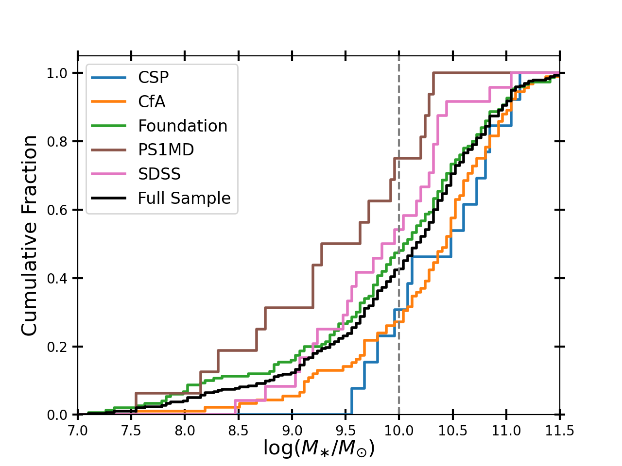
Figure 1: Cumulative distributions of host-galaxy masses for the different surveys included in the training sample. Approximately 75% of our masses are from the Foundation and CfA samples.

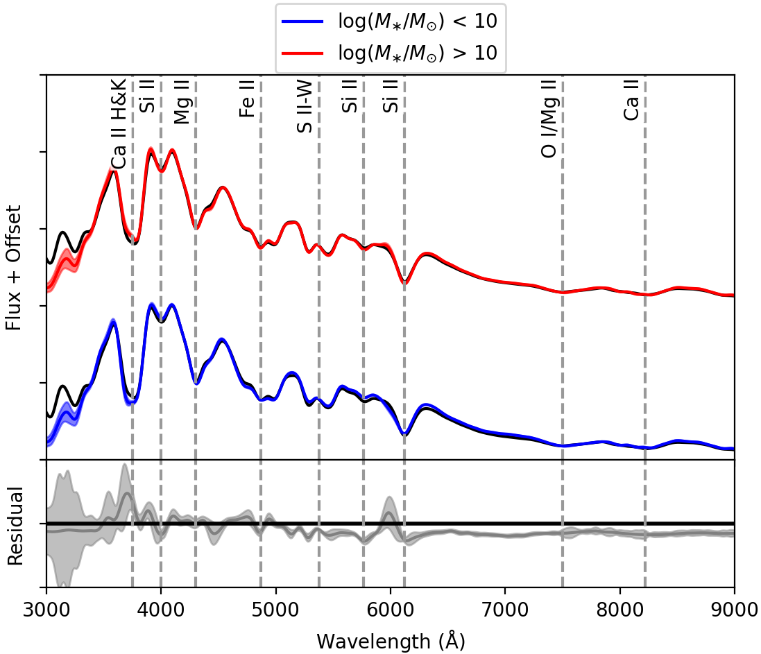
Figure 2: Top: the average spectrum of a $(x_{1},c)=(0,0)$ SN Ia at maximum light for SNe in high-mass (red) and low-mass (blue) host galaxies. The $(x_{1},c)=(0,0)$ spectrum from K21 is in black. Bottom: the difference between the red and blue spectra in the top panel, equal to the $M_{host}$ component from Equation 2. We note that both models differ from K21 in the blue due to the removal of high-redshift, rest-frame UV data.

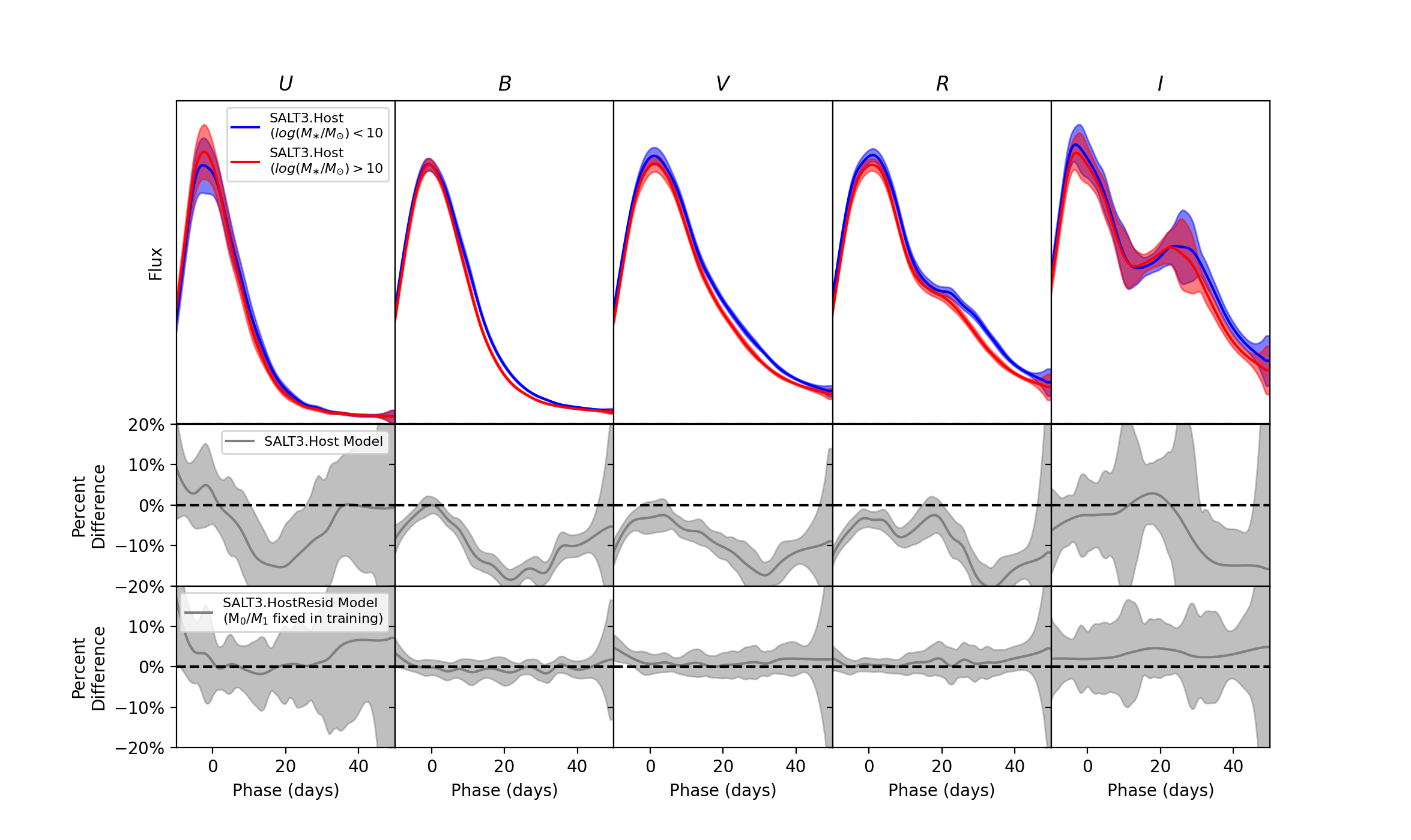
Figure 3: Top: $U\!BV\!RI$ light curves of the mean SN Ia in a high-mass (red) vs. low-mass (blue) host galaxy from the SALT3.Host model ($M_{0}\pm 0.5M_{host}$). The $y$-axis is scaled from zero to $+$130% of the flux at maximum light in the high-mass light curve for each band; note that red and blue curves are normalized by SALTshaker to have the same flux at $B$-band maximum light. Middle and bottom: residual curves for the difference between SNe in high- and low-mass hosts for the SALT3.Host model (middle) and the SALT3.HostResid model (bottom).

Figure 4: Same as Figure 3 but for top-hat filters centered on the Si II lines at rest-frame 4130 and 6355Å. To cover the full lines while avoiding nearby absorption features, we use filters from 3900 to 4100 Å and 6000-6250 Å, respectively (Si II is blueshifted from its rest frame in SNe Ia). We note that there is greater noise in the line-profile light curves than in the broadband light curves in Figure 3.

2.3 Measuring Host-Galaxy Masses

We measure host-galaxy masses for SNe in our training sample by first using the Galaxies HOsting Supernova Transients (GHOST; Gagliano et al., 2021) software to determine the host galaxy for each SN. GHOST uses a gradient-ascent algorithm to match SN locations to their likely host galaxies using deep PS1 postage-stamp images at each SN location. Next, we visually inspect the GHOST matches, and alternatively use the SExtractor-based “directional light radius” (DLR) method (Sullivan et al., 2006; Gupta et al., 2016) on $r$-band images from Pan-STARRS (PS1; Chambers et al., 2016) to correct the few percent of erroneous matches. Finally, for SNe with no identifiable host either visually or with GHOST, we assume the true host is at the SN location; at $z<0.15$, hosts that are undetected in PS1 imaging will all have ${\rm log(M_{\ast}/M_{\odot})}<10$, but we use their location for photometric measurements in case upper limits on the mass are needed for future work.

With these host-galaxy locations, we use SExtractor (Bertin & Arnouts, 1996) to measure the isophotal elliptical radius of each galaxy, again using PS1 $r$-band imaging. We measure photometry within this radius using images from GALEX, the Sloan Digital Sky Survey (SDSS), PS1, and 2MASS, modifying the radius slightly to account for the changing size of the point-spread function (PSF) for each filter and instrument (Table 2).

Finally, we use LePHARE (Ilbert et al., 2006) to measure the host-galaxy masses of each SN. We used the Chabrier (2003) initial mass function and the Bruzual & Charlot (2003) SED template library. The extinction $E(B-V)$ is varied from $0$-$0.4$ mag. The resulting host-galaxy mass distributions for each subsample in our analysis are shown in Figure 1.

3 Results

The SALT3.Host model is illustrated in Figure 2 for spectra at maximum light and in Figure 3 for $U\!BV\!RI$ light curves. The phase-dependent evolution of the Si II lines are shown in Figure 4 and the (small) differences in color laws between models are shown in Figure 5. The full $M_{host}$ spectral component is shown in Figure 6 for the SALT3.Host model and in Figure 7 for the SALT3.HostResid model. Finally, the phase-dependent $B-V$ colors of the SALT3.Host model are shown in Figure 8.

Below, we discuss the characteristics of these surfaces. We note that uncertainties in the light curves are well correlated on scales of $\sim$3 days, but are largely independent over longer timescales. In addition, the figures and analysis in this section use only the out-of-sample (bootstrapped) uncertainties, as these are the formal statistical uncertainties on the determination of the model surfaces. We include in-sample variance in the distance fitting (Section 3.3).

3.1 Model Spectra and Light Curves

We first examine the SALT3.Host model, and find that spectra at maximum light have significantly different Ca H&K and Si II (6355Å) line profiles as a function of host-galaxy mass. In particular, SNe in low-mass hosts have broader absorption features on average (Figure 2); at maximum light, we measure larger Ca NIR triplet, Ca H&K and Si II equivalent widths at 2.7-, 2.3-, and 2.2-$\sigma$ significance, respectively, which are correlated with higher velocities and explosion energies per unit of SN mass (e.g., Wang et al., 2009; Zhao et al., 2015). The Ca H&K velocity is higher in low-mass hosts, but at just 1.3-$\sigma$ significance, and there is no difference in the Si II velocity. While the significance of these results could be somewhat enhanced by the look-elsewhere effect, we note that previous studies have specifically investigated differences in Si II and Ca H&K absorption features as potentially correlated with Hubble residuals (Foley & Kasen, 2011; Siebert et al., 2020), so we have a priori reasons to suspect host-dependent changes in these line profiles.

Additional spectral differences are observed at later phases, particularly in the Si II features (Figures 4 and 6). The differences in light-curve properties are not limited to places where spectral features are expected to vary (e.g., we observe qualitatively similar behavior at $\sim$4500-5000Å), but variation in these Si II and other absorption features could explain some of the variation present in the broadband light curves. We also see other differences between the high-mass host galaxy and low-mass host galaxy SN models at 25–35 days (Figures 3 and 6), near the time of NIR maximum light, which is an epoch that could be particularly sensitive to the metallicity of the SN progenitor (Kasen, 2006).

In Figure 3, we also confirm previous results that SNe Ia in high-mass hosts have narrower shapes on average than those in low-mass hosts (e.g., Hamuy et al., 2000; Gallagher et al., 2005), as well as an earlier time of secondary maximum light (Figure 3). Significant phase-dependent color differences as a function of host mass can be seen (Figure 8), which were previously captured as part of the SALT3 $M_{1}$ component and represented by the SALT3 $x_{1}$ component in light-curve fits.

Lastly, we note that the updated $M_{1}$ component appears qualitatively similar to the SALT3.HostIgnore model, but with larger-amplitude $x_{1}$-dependent color changes, particularly near maximum light (these are phase-dependent colors and can therefore be separated from the phase-independent color law).

We compare these SALT3.Host results to light-curve residuals and spectra from the SALT3.HostResid model in Figures 3 and 4 (bottom panels) and Figure 7. Near maximum light, we see that previous SALT models have not fully accounted for variations in the Ca H&K and Si II absorption features between different host-galaxy types. There is also a slight possibility of increased amplitude of the host-mass component in the $I$ band, indicated by the persistent low-significance offset in the bottom-right panel of Figure 3. Overall, however, the pre-existing $M_{1}$ surface had encoded most of the host-dependent variation in SN properties, and the amplitudes of the spectral changes in Figure 7 are significantly smaller than those in Figure 6.

3.1.1 Colors

In Figure 8, we show the evolution of $B-V$ synthetic color for the SALT3.Host model. We see significantly different color evolution from $\sim$10 to 20 days after maximum light; the evolving color difference may indicate that these colors are intrinsic to the SNe. We note that qualitatively similar behavior is seen in Figure 11 of Siebert et al. (2020), when comparing SNe with negative (preferentially high-mass hosts) versus positive (preferentially low-mass hosts) Hubble residuals.

The SALT3.HostResid model, on the other hand, has a statistically insignificant color shift (Figure 3), implying that adding a host-galaxy mass component to the SALT model has a negligible effect on the fitted broadband light curves of a given SN. We do note that if the persistent low-significance color shift in the $I$ band shown in Figure 3 is both real and due to extrinsic dust, it may imply lower $R_{V}$ for high-mass galaxies as predicted by Brout & Scolnic (2021).

Finally, we note that the trained color law itself is nearly identical in the SALT3.Host model as it is in the model without a host-galaxy component (SALT3.HostIgnore); for a red SN of $c=0.1$, for example, the difference in color laws would amount to a change in flux of less than 0.5% at any wavelength (Figure 5).

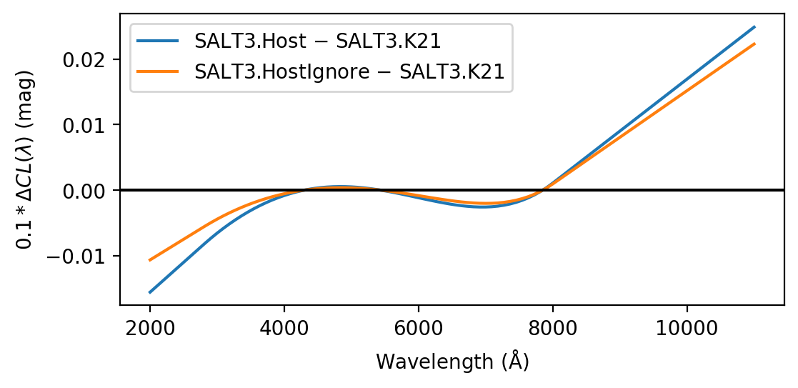
Figure 5: Difference in color laws for a $c=0.1$ SN between K21 and the SALT3.Host (blue) and SALT3.HostIgnore models (orange; note that the SALT3.HostResid model has the same color law as SALT3.HostIgnore by construction). SALT3.Host and SALT3.HostIgnore differ at the mmag level at the bluest and reddest wavelengths.

3.2 Model Validation

By using the Bayesian information criterion with the log-likelihood returned by SALTshaker, we find that the SALT3.Host model is heavily favored over the SALT3.HostIgnore model, which is trained using the original SALT formalism on the same data set. However, we find that the likelihood of the photometric data alone changes less significantly between SALT3.HostIgnore and SALT3.Host, as discussed in Section 3.3 below.

To ensure that host-galaxy-dependent differences are not due to systematic errors in the SALTshaker training procedure, we use randomly assigned masses to train “random” versions of the SALT3.Host model, finding that only low-significance changes in spectral features are recovered. Those results are presented in the Appendix.

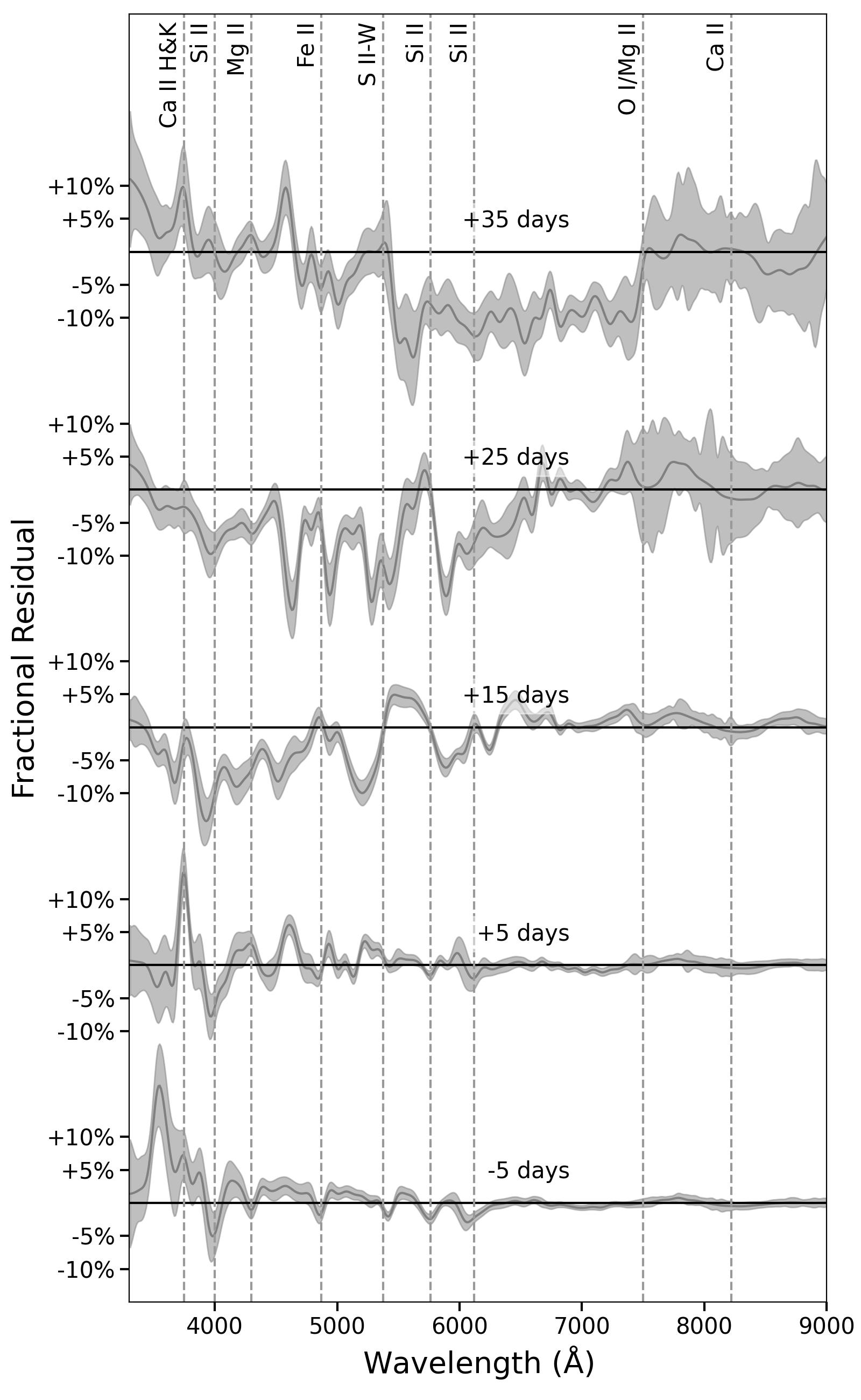
Figure 6: The evolution of the host-galaxy mass component of the SALT3.Host spectral model with phase, which can be interpreted as the mean spectrum of a SN Ia in a high-mass galaxy minus the mean spectrum of a SN Ia in a low-mass galaxy. At each phase, we show $M_{host}$ as a fraction of the corresponding $M_{0}$ flux at 4300Å (approximately the $B$-band wavelength). Variation in the line profiles, particularly those of the Ca H&K and Si II features, are observed across many phases. The tilt (color) of the spectrum also changes significantly with phase.

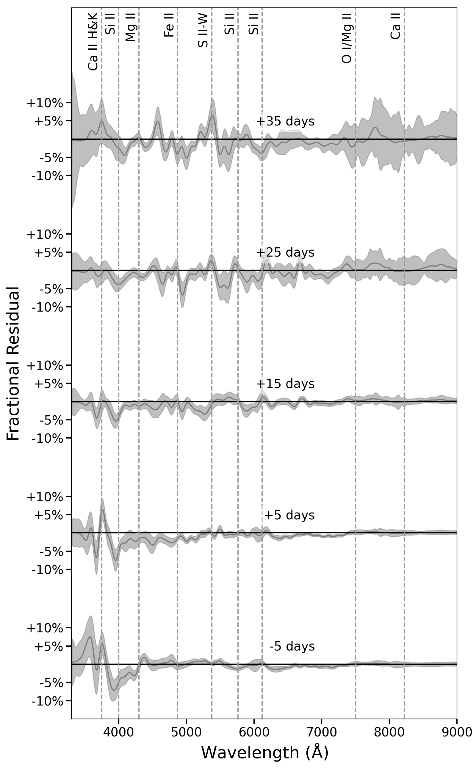
Figure 7: The same as Figure 6, with the same y-axis scale, but for the SALT3.HostResid model. This model shows only the host-mass-dependent spectral component that is “missing” from previous SALT2 and SALT3 models. Significant spectral fluctuations are observed near maximum light in the vicinity of Ca H&K, but few statistically significant deviations are seen at redder wavelengths and later phases.

3.3 Distance Measurements

Next, we use the SNANA software (Kessler et al., 2010) to fit the photometric training data with the SALT3.Host, SALT3.HostResid, and SALT3.HostIgnore models. We apply selection cuts on redshift, $x_{1}$ and $c$ ($z>0.01$, $-3<x_{1}<3$, and $-0.3<c<0.3$, following Scolnic et al., 2018), after which 261 of the original 296 SNe remain for measuring distances.

We subsequently estimate nuisance parameters and distances from the Tripp estimator (Tripp, 1998):

$$\mu=m_{B}+\alpha\cdot x_{1}-\beta\cdot c-\mathcal{M}.$$ (3)

The $\alpha$ and $\beta$ variables are nuisance parameters that standardize the SN brightness and are determined in a global fit using SNANA’s SALT2mu method (Marriner et al., 2011). $\mathcal{M}$ is the absolute magnitude of a SN Ia, which is set to a nominal value in this work, and $m_{B}$ is the log of the fitted light-curve amplitude. The mass step, $\Delta_{M}$, can be included in this equation, but we treat it separately in this work. Additionally, bias corrections to correct the measured $\mu$ for selection effects as a function of redshift are commonly included in the Tripp estimator but are not necessary here; we only examine the differential distance measurements between models and therefore this term cancels to first order.

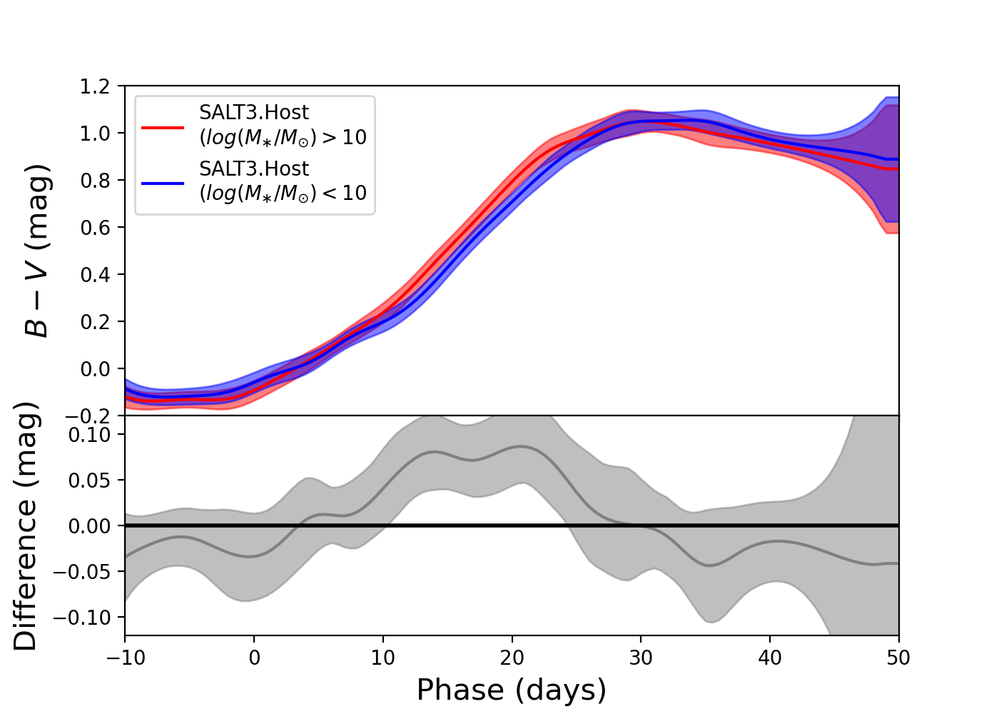
Figure 8: The $B-V$ color of the SALT3.Host model in high- and low-mass host galaxies (top) and the difference between the two (high-mass minus low-mass colors; bottom). There is significantly different color evolution from $\sim$10 to 20 days for SNe Ia in low- vs. high-mass hosts, which can also be seen when comparing the different light-curve shapes in Figure 3. We note that the red and blue curves in the top panel include the $M_{0}$ uncertainty, while the residual curve neglects this correlated error and shows only the uncertainty on the difference (the $M_{host}$ error).

Table 3: SALT3 Light-Curve Fitting $\chi^{2}$, Hubble Residual rms, and Nuisance Parameter Comparisons

Version	HR rms	LC $\chi^{2}/\nu$ a	$\alpha$	$\beta$ b	$\Delta_{M}$
	(mag)				(mag)
SALT3.HostIgnore	0.145	1.49	$0.133\pm 0.009$	$2.675\pm 0.092$	$0.057\pm 0.018$
$-$ $\rm log(M_{\ast}/M_{\odot})<10$	0.140	1.49	$0.133\pm 0.016$	$2.900\pm 0.140$	$\cdots$
$-$ $\rm log(M_{\ast}/M_{\odot})>10$	0.147	1.49	$0.149\pm 0.011$	$2.552\pm 0.119$	$\cdots$
SALT3.HostResid	0.148	1.48	$0.137\pm 0.009$	$2.616\pm 0.093$	$0.032\pm 0.019$
$-$ $\rm log(M_{\ast}/M_{\odot})<10$	0.151	1.47	$0.124\pm 0.015$	$2.828\pm 0.145$	$\cdots$
$-$ $\rm log(M_{\ast}/M_{\odot})>10$	0.147	1.50	$0.153\pm 0.011$	$2.482\pm 0.119$	$\cdots$
SALT3.Host	0.144	1.45	$0.132\pm 0.009$	$2.659\pm 0.090$	$0.036\pm 0.019$
$-$ $\rm log(M_{\ast}/M_{\odot})<10$	0.141	1.44	$0.125\pm 0.020$	$2.910\pm 0.134$	$\cdots$
$-$ $\rm log(M_{\ast}/M_{\odot})>10$	0.146	1.49	$0.137\pm 0.011$	$2.549\pm 0.119$	$\cdots$
a Neglecting model uncertainties and color dispersion terms, which are estimated such that each model has a reduced $\chi^{2}\simeq 1$. To avoid biases to the $\chi^{2}$, we add a 0.1% error floor to the data uncertainties and omit $z$- and $U/u$-band data because they have significantly higher model uncertainties than the rest of the wavelength range. b With SALT2.4 (Betoule et al., 2014), we measure a consistent $\beta=2.73\pm 0.099$ from this sample, slightly lower than typical analyses including high-$z$ SNe ($\beta\simeq 3$; Scolnic et al., 2018).

We report the measured nuisance parameters $\alpha$, $\beta$, and $\Delta_{M}$ in Table 3. Each parameter is computed both for the complete sample and for SNe in high-mass and low-mass host galaxies separately. We also report the rms dispersion of Hubble residuals for each model. We see statistically insignificant differences of just $\sim$0.01 in the $\alpha$ parameter and $\sim$0.005 in the $\beta$ parameter between SALT3.Host and SALT3.HostIgnore. Between low-mass and high-mass hosts, however, we see marginally significant differences of $\sim$0.015-0.02 in $\alpha$ and $\sim$0.35 in $\beta$, suggesting that fitting $\alpha$ and $\beta$ separately for these samples might reduce distance uncertainty and perhaps cosmological bias (Kelsey et al., 2022). After subtracting the $\Lambda$CDM cosmological model prediction from Planck Collaboration et al. (2018), we see a consistent Hubble residual RMS for all three models.

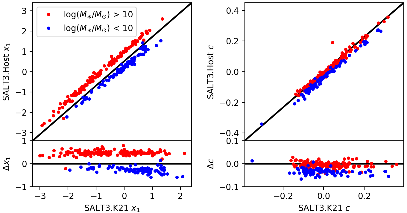
Figure 9: Comparing the $x_{1}$ (left) and $c$ (right) parameters measured from SALT3.Host versus the SALT3 model from K21. Low-mass host galaxies are shown in blue and high-mass hosts are in red. Residuals are shown in the bottom panels. The large difference in measured $x_{1}$ (left panels) is due to the removal of the $x_{1}$–host mass correlation present in previous SALT models.

To compare SALT3.Host to the previously published SALT3 model (K21), we show the $x_{1}$ and $c$ parameters measured with each model in Figure 9. The addition of a host-galaxy mass component changes the definition of $x_{1}$ such that there is a much lower mean difference in $x_{1}$ between high- and low-mass host galaxies for SALT3.Host ($\simeq 0.17$) compared to the SALT3 model from K21 ($\simeq 0.91$; hereafter SALT3.K21). The marginally significant host-dependent variation in the $\alpha$ parameter (0.015-0.02) seems to suggest that the $x_{1}$–luminosity relation is changing slightly between different host types.

Interestingly, the mean color of SNe in high-mass hosts is slightly more red ($\simeq$0.05) in SALT3.Host compared to SALT3.K21 ($\simeq$0.03; Figure 9). This may mean that some variation in the dust color law or the intrinsic colors of SNe that was not previously modeled may have been captured by the new $M_{host}$ component.

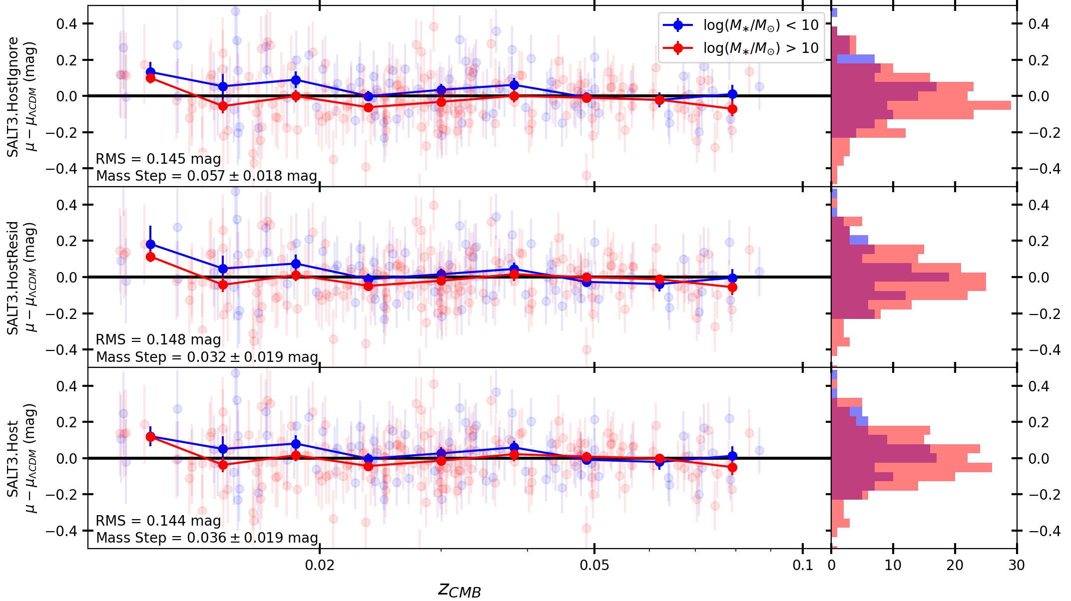
Figure 10: From top to bottom, Hubble residuals for the SALT3.HostIgnore model, the SALT3.HostResid model, and the SALT3.Host model. Blue points show Hubble residuals of SNe in low-mass host galaxies, while red points show Hubble residuals of SNe in high-mass hosts. The size of the mass step is decreased by $0.021\pm 0.002$ mag when adding a host galaxy component to the SALT model framework.

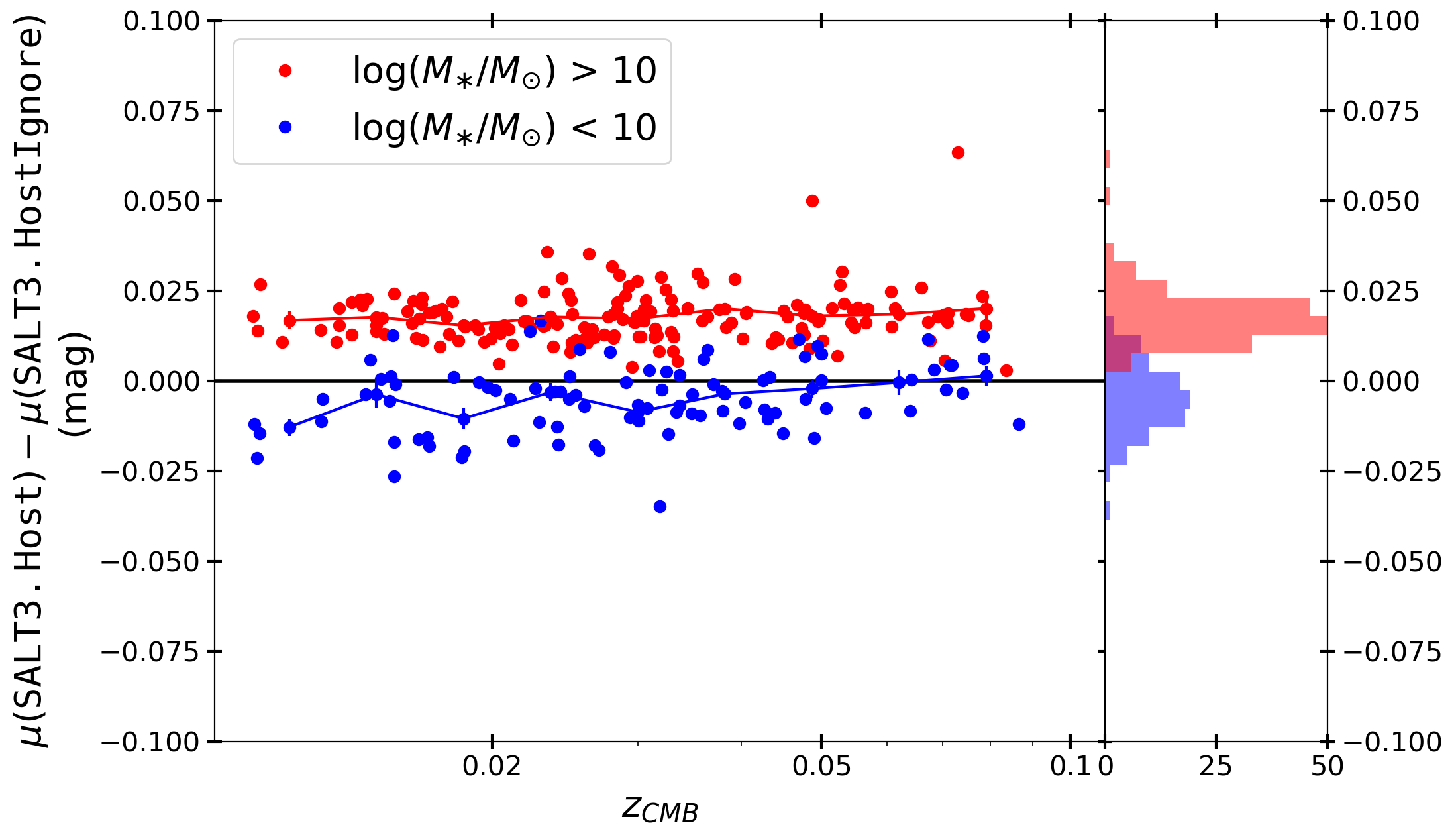
Figure 11: Difference in Hubble residuals for high-mass-hosted SNe (red) and low-mass-hosted SNe (blue) between the SALT3.Host and SALT3.HostIgnore models. Corresponding differences in $x_{1}$ and $c$ parameters are shown in Figure 9.

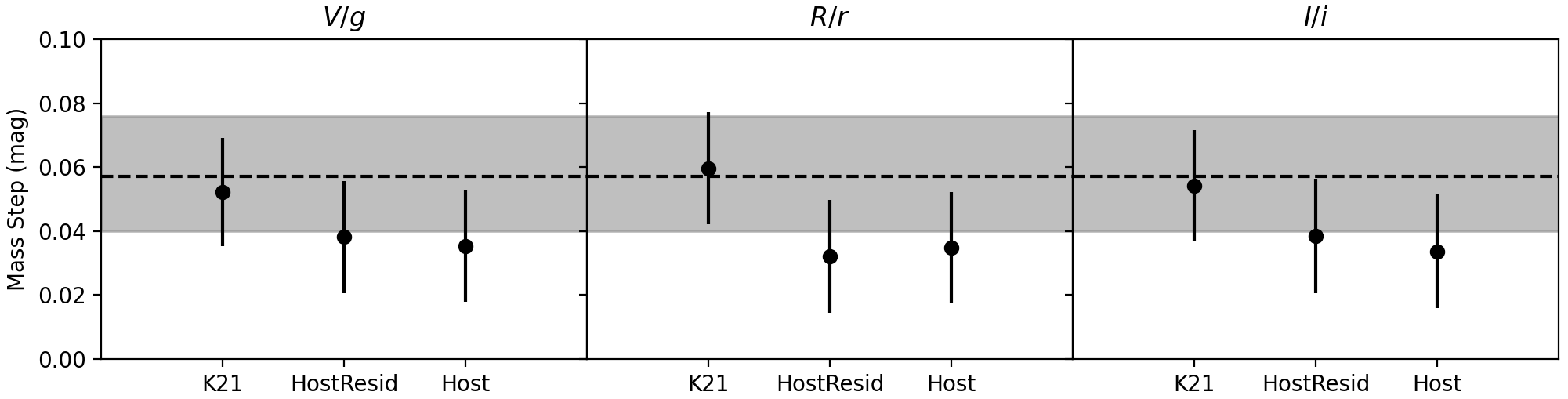
Figure 12: Mass steps measured by using $x_{0}$ parameters measured from the $V/g$ bands only (left), the $R/r$ bands only (center), and the $I/i$ bands only (right) for the SALT3 model from K21, the SALT3.HostResid model, and the SALT3.Host model. The gray dashed line and shaded region is the best-fit value and uncertainty from the full data set fit with the SALT3.K21 model. Values of the $x_{1}$ and $c$ parameters are determined using a global fit to all available data for each SN. Mass step measurements appear to be wavelength-independent within the measurement noise but we cannot rule out significant variation.

3.3.1 The Host-Galaxy Mass Step

We measure the host-galaxy mass step by following the approach outlined in Jones et al. (2018) that incorporates both Hubble residual and host-galaxy mass uncertainties. Jones et al. (2018) construct a model to find the maximum-likelihood value of the step by assuming two Gaussian SN populations in Hubble residual space; the means and dispersions of these Gaussians are free parameters (see also Rigault et al., 2015 and Jones et al., 2015). The model takes into account that each SN has a probability of being in either a high-mass or low-mass host galaxy, which is given by the probability distribution function of the host-galaxy mass measurement.

From the SALT3.HostIgnore model, we measure a mass step of $0.057\pm 0.018$ mag versus $0.036\pm 0.019$ mag from the SALT3.Host model (Figure 10). After recomputing the mass step with 100 bootstrap iterations of the SN sample, which takes into account the fact that the same data are used for both mass-step measurements, we find that the mass step is reduced by a highly significant $0.021\pm 0.002$ mag when the SALT3.Host model is applied.

Even with the SALT3.Host model, the mass step remains significant at the $\sim$2-$\sigma$ level. This implies a significant difference in the shape- and color-corrected $B$-band absolute magnitude of SNe Ia as a function of host mass even after explicit modeling of the SN Ia–host mass relation in a luminosity-independent way. Given the low uncertainties on the mass-step difference above, we consider it likely that larger samples would measure the mass step with high statistical significance even when using the SALT3.Host model.

In Figure 11, we show the difference in Hubble residuals between the SALT3.Host and SALT3.HostIgnore models. Both the SALT3.Host and SALT3.HostResid models change the Hubble residuals by shifting the measured color parameter $c$ (Figure 9); this appears to be because some color differences previously attributed to the global, phase-independent color are now determined by SALTshaker to be dependent on host properties. Additionally, the SALT3.Host model changes the measurement of $x_{1}$ and therefore some $x_{1}$ differences are now modeled as part of the host component. The measured $m_{B}$ does not change significantly in either model, which is unsurprising given that $m_{B}$ is defined to be the same at maximum light for both models.

These results show that our host-dependent SN Ia model alters the determinations of color and first-order variability, which in turn causes the mass step to shrink. These redefined terms appear to improve the Hubble residual scatter very slightly, and we find specifically that there is less Hubble residual scatter due to the $\alpha x_{1}$ or $\beta c$ terms in the Tripp equation when applying the SALT3.Host framework (a small $\sim$1-2% improvement). Our distance fitting and mass-step results are summarized in Figure 10 and Table 3.

3.3.2 Light-Curve Fitting Residuals

We find that the light-curve fit residuals themselves are only weakly affected by the choice in model, as shown in Table 3. When model uncertainties are completely excluded from the $\chi^{2}$ computation, we see that the median reduced $\chi^{2}$ values for the $B$, $V$ and $R$ bands are slightly reduced by $\sim$0.03-0.05. The difference in total $\chi^{2}$ between models is a statistically significant $\Delta\chi^{2}=480$, but the effect on an individual SN Ia light curve is small.

In addition, the median $I$ and $z$ reduced $\chi^{2}$ values increase slightly in the SALT3.Host model (wavelengths at which model errors are significantly larger). We note that the total photometric $\chi^{2}$ for $z$-band photometry is slightly lower for the SALT3.Host model, but the median reduced $\chi^{2}$ per SN is slightly higher, showing that some SNe have much larger contributions to the total $\chi^{2}$ than others. The SALT3.HostResid model has a lower photometric $\chi^{2}$ in every band compared to SALT3.HostIgnore, but the $\chi^{2}$ is larger overall than it is for SALT3.Host.

3.3.3 The Wavelength Dependence of the Mass Step

Finally, we explore the wavelength dependence of the mass step by performing a global mass-step fit to the SN data using the SALT3.K21 model, the SALT3.HostResid model, and the SALT3.Host model. Next, we use the global $x_{1}$ and $c$ parameters measured using a fit to all bands for each SN, but generate amplitudes ($x_{0}$) from the $V/g$ bands, the $R/r$ bands, and the $I/i$ bands separately. The goal is to see if the mass step changes significantly in different bands, with the different models explored here, and within the wavelengths covered by the SALT model. The results are summarized in Figure 12.

For the K21 model, the mass step is consistent with no wavelength dependence, but we cannot rule out significant variation. Although well within the statistical errors, the mass step is very slightly larger in the $R/r$ and $I/i$ bands than it is in the $V/g$ bands, as would be predicted from Figure 3. Counterintuitively, a larger mass step at red wavelengths is consistent with a lower $R_{V}$ in high-mass hosts, as the amplitude of a SN in these redder bands is extrapolated to the $B$ band assuming the host-independent SALT3.K21 model. We also see again that the addition of the host-galaxy mass component reduces the mass step by $\sim$0.02 mag; as the mass component is normalized to be equal to zero at $B$-band maximum light, this reduction cannot be due to luminosity information encoded in the mass step (e.g., dust extinction differences or other physical mechanisms that change the $B$-band SN luminosity).

We also investigate the dependence of the Hubble residual rms on the color parameter $c$ to see if the trend of increased color scatter with $c$ observed by Brout & Scolnic (2021) is altered by applying the SALT3.Host model. We see no significant change, with both sets of distance residuals from SALT3.HostIgnore and SALT3.Host having an rms that increases from $\sim 0.13$ mag at $c\simeq-0.05$ to $\sim 0.16$ mag at $c\simeq 0.1$, indicating that adding a single host-mass component does not significantly affect the increased color scatter of red SNe. This result is consistent with the Brout & Scolnic (2021) model, as our correction to the mean of the flux would be incapable of substantially addressing the variance caused by a large diversity of extinction laws.

The measured $\beta$ parameter between low- and high-mass hosts differs by $\sim$0.35 across all models, with high-mass-hosted SNe preferring lower values of $\beta$. This is again consistent with the prediction of lower $R_{V}$ in high-mass hosts (Brout & Scolnic, 2021).

4 Discussion

It has long been known that the SALT framework is an incomplete method of standardizing SNe. Light-curve models such as SNEMO (Saunders et al., 2018) demonstrated that additional principal components can improve SN Ia distances, and the addition of more sophisticated distance measurement tools have been shown to decrease the size of the mass step (Boone et al., 2021b). Work from Rose et al. (2020) and Rubin (2020) indicate that the optimal number of standardization parameters for SN Ia distance measurement is greater than the number currently included in SALT. Furthermore, the recently developed SUGAR model (Léget et al., 2020), a principal-component-based method with higher-order terms than SALT, also shows spectroscopic differences with SALT near the locations where the SALT3.Host model differs (particularly near Ca H&K and the Si II feature at 6355Å). Finally, given the known dependence of stretch and color on SN Ia host-galaxy properties, it is unsurprising that not all spectral dependencies were previously modeled by SALT.

In spite of these complexities, the mass step is typically modeled as a wavelength-independent parameter, which is perhaps part of the reason that different data sets covering different rest-frame wavelength ranges produce different mass-step measurements (e.g., Brout et al., 2019). This work provides a full spectrophotometric model of the mass step, which could be shifted to have a $B$-band magnitude of $0.036$ — a reduction of $0.021\pm 0.002$ mag compared to a SALT3 model without host-galaxy information — to yield a mass step of zero. Additionally, this shift applied to our SALTshaker training results should cause the measured absolute magnitude difference at every phase and wavelength between a mean SN Ia in a high- versus low-mass host galaxy to be equal to zero. While much of this host-dependent variation was previously encoded by the $x_{1}$ parameter in previous SALT models, our SALT3.HostResid model shows that there are still subtle but statistically significant spectral differences (Figures 4 and 7) and possibly subtle color differences (Figure 3, bottom panel) between high- versus low-mass-hosted SNe that were not captured by the previous SALT formalism.

4.1 Implications for SN Ia Distance Measurement Methods

Given the uncertainty in SN Ia physics and progenitor systems, a model that depends only on the host-galaxy mass is unlikely to be truly optimal for cosmological distance fitting. Alternative SALT3 models that depend on specific star formation rate, progenitor age, or other properties could be used within the SALT3.Host framework. However, all of these models will be subject to uncertainty regarding whether they remain valid as a function of redshift as SN Ia progenitors and host-galaxy dust properties evolve. A logical additional extension would be to incorporate the full host-galaxy parameter probability distribution functions as priors into the model training, allowing a model to be trained as a function of galaxy properties that have larger uncertainties.

Given that the SALT3.Host does not yield clear differences in Hubble residuals or improvements in dispersion, and only results in a small improvement in the quality of the light-curve fits themselves, it may be appropriate to continue using the simpler model formalism of the SALT3.HostIgnore model for cosmology. However, for measuring $w$, the leverage that the SALT3.Host model provides may be extremely useful as a systematic test that helps us understand the wavelength ranges, redshifts, and filter sets that are particularly sensitive to the observed spectral variations as a function of host-mass properties. As the model itself can be trained at any redshift, it is also possible to measure whether the SN Ia–host mass correlation is evolving with redshift as a function of both wavelength and phase.

Finally, the lack of a large difference in the goodness-of-fit statistic when comparing SALT3.Host to SALT3.HostIgnore is somewhat surprising given that both SN Ia spectra and light curves vary significantly as a function of their host-galaxy properties. Given that spectra are more homogeneous in particular host-galaxy types, this result may limit the precision one could expect from a “twinning” approach in which SNe with similar spectra are compared to yield more precise relative distance estimates (e.g., Fakhouri et al., 2015; Boone et al., 2021b). However, it is possible that modeling the SN spectra as a function of alternative global or local host-galaxy properties might result in more drastic improvements to Hubble residuals.

4.2 Implications for SN Ia Physics

The SALT3.Host model gives a more precise understanding of the ways in which a mean SN Ia spectrum changes depending on its host galaxy. Though the dependence of SN Ia properties on host-galaxy properties is already well known, by constraining the host dependence at the same time as the principal-component-like $M_{0}$ and $M_{1}$ surfaces and phase-independent color law, our model is constructed in such a way that it separates the component of SN Ia intrinsic diversity uncorrelated with host mass from the change in mean properties as a function of host mass.

At 1.3-$\sigma$ significance, we find evidence that the Ca H&K velocity is less blueshifted in higher-mass hosts, indicating at low significance — and contrary to results from composite spectra in Siebert et al. (2019) — that SNe in higher-mass host galaxies may have lower explosion energies per unit mass (the difference could be due to our more robust prescription of controlling for intrinsic variation when comparing high- to low-mass-hosted SNe). Similar evidence is seen from the larger observed equivalent widths in the Ca NIR triplet, Ca H&K, and Si II line profiles, at 2.7-, 2.3-, and 2.2-$\sigma$ significance. At late times, we note that Siebert et al. (2020) found evidence for larger equivalent widths in spectral features for SNe with positive Hubble residuals (more likely to be low-mass hosts), which aligns with our results from spectra nearer to peak. Siebert et al. (2019) also saw hints of increased Ca H&K and Si II absorption in late-type galaxies, which is consistent with our findings. Finally, we see that the $I$-band secondary maximum may be slightly earlier relative to the peak flux, which would indicate a larger synthesized mass of electron-capture elements in high-mass hosts (Kasen, 2006). As a caveat, we note that the Ca H&K line may be blended with Si II at 3858Å (Foley, 2013), which may have some effect on the Ca H&K results.

Building this model as a function of other host-galaxy parameters may help to isolate additional physical processes in SN Ia explosions that depend on the metallicity or progenitor properties that are more prevalent in certain galaxy types. We hope that this approach will be effective at isolating subtle SN Ia physical behaviors with the use of large samples. We also hope that future investigations can continue to explore the ways in which differences in, for example, explosion energies, could affect the spectra, light curves, and luminosities of SNe in cosmological samples.

4.2.1 Constraining the Role of Dust in the SN Ia Mass Step

Brout & Scolnic (2021) predicted that the mass step is caused by reddening law variation in SN Ia hosts. To generate this prediction, they modeled SN Hubble residual data assuming a symmetric intrinsic color distribution and a one-sided reddening law to break the degeneracy between intrinsic and extrinsic colors. In the SALT3.Host model, on the other hand, we do not have the ability to conclusively separate intrinsic and extrinsic colors. Although some substantial color differences appear to be phase dependent (Figure 8), showing that intrinsic colors vary with host mass, the degree to which extrinsic colors vary is not clear from this model.

To break this degeneracy, we would require a more sophisticated treatment of color within the SALT3 framework. Expanding the SALT3.Host model further by training two separate color laws for low- and high-mass host galaxies might help us to understand the degree to which a phase-independent SN color term is evolving between different galaxy types. In addition, a SALT3 model that also includes NIR wavelengths to anchor the color, e.g., Pierel et al. (2022), will also contribute to a better understanding of the role of SN color in causing the apparent host-mass step.

Lastly, because the host-galaxy component of the SALT3.Host model is shifted to have zero $B$-band flux, applying the SALT3.Host model cannot correct for physical processes that affect the $B$-band luminosity. Therefore, the $\sim$0.02 mag reduction in the host-galaxy mass step when using the SALT3.Host model implies that a small but significant fraction of the mass step likely cannot be explained by reddening law differences.

4.3 Caveats

The training sample used here is subject to significant selection effects. In particular, approximately half the data are comprised of samples that were chosen from a preselected set of bright galaxies; controlling for the mass step alone may not sufficiently remove the biases in this sample as a function of host-galaxy properties. The way in which the demographics of those data could affect the recovered spectral model are difficult to fully understand from our limited data set; however, these data are the same as those used in other recent SALT model trainings (e.g., Betoule et al., 2014; Kenworthy et al., 2021; Taylor et al., 2021), meaning that these types of biases are already present in existing models used for SN Ia cosmology studies.

Despite these selection effects, spectroscopic data are important for models that explore the spectroscopic dependence of the SALT3 model on host-galaxy properties, and there exists no high-S/N sample of SN spectra comparable to the one that has been assembled over the last three decades at low redshift. Replacing this sample with future, less biased spectroscopic data sets will take considerable work.

SALTshaker also does not yet have a process to correct the data or model for observational biases, which could potentially be addressed by a fitting process that includes an iteratively updated, simulation-based bias-correction process to refine, for example, $x_{1}$ and $c$ estimations and correct the resulting model surfaces for biases in those parameters. Understanding the role that such biases could play in the training process are an important consideration for future work (Dai et al., 2022).

Lastly, our data set remains limited redward of $\sim$7000-8000Å. Foundation alone has rest-frame $z$-band data to constrain, for example, the SN model in the vicinity of the Ca II NIR triplet. However, ongoing surveys such as the Young Supernova Experiment (Jones et al., 2021) and future surveys including the Rubin Observatory’s Legacy Survey of Space and Time will supplement these data and — with additional spectroscopic follow-up observations — allow a better understanding of spectroscopic behavior at longer wavelengths. Additionally, recent SN Ia NIR model extensions and spectroscopic data releases (Lu et al., 2022; Pierel et al., 2022) will help to constrain the model’s dependence on host-galaxy properties at $YJH$ wavelengths in the near future.

5 Conclusions

In this work, we expand the SALT3 framework by building a wavelength- and phase-dependent model of the SN Ia dependence on host-galaxy mass. We observe variations in SN Ia spectral features and colors that were not previously captured by the SALT modeling framework. We also observe a complex dependence of SN Ia light curves and spectra on their host-galaxy properties. We hope that this modeling framework can be used to better understand how cosmological parameter measurements and SN selection effects may be systematically affected by the wavelength and phase dependence of the SN Ia—host galaxy relation.

This revised model has a significantly higher likelihood given the SN Ia data, though it does not appear to reduce the Hubble diagram RMS dispersion. It does, however, reduce the size of the mass step by $0.021\pm 0.002$ mag, where errors take into account the fact that the same data are used with both the SALT3.Host and SALT3.HostIgnore models. This indicates that $\sim$35% of the mass step is due to luminosity-independent effects. Furthermore, if the host-galaxy component is shifted such that it has a $B$-band magnitude of $+$0.036 mag at maximum light, the size of the mass step in SN Ia distance fitting becomes consistent with zero. However, this value must be determined by a Hubble residual analysis and cannot be estimated by the luminosity-independent SALTshaker model training process.

We see evidence for less energetic SN Ia explosions per unit mass in high-mass host galaxies, and marginal evidence for an earlier epoch of secondary maximum light that could have implications for the physics of the explosions. We find moderate, phase-dependent differences in color between SNe in high- and low-mass hosts that — due to their phase dependence — are likely intrinsic. We hope this model, and future models constrained with additional data, will offer additional insight into the physics of SN Ia explosions in both the nearby universe and as a function of redshift.

This revised modeling framework also directly constrains the SN Ia host-galaxy mass dependence in a way that was not previously possible with existing data. It is capable of testing the redshift dependence of SN Ia spectra and the redshift evolution of the spectrally resolved relationships between SNe Ia and their hosts. Future data sets with high-cadence, high-S/N spectral sequences will help to better constrain the dependence of SNe Ia on their host-galaxy masses and other physical parameters in order to better pinpoint the physics responsible for the mass step and improve the precision of distance measurements in cosmology analyses.

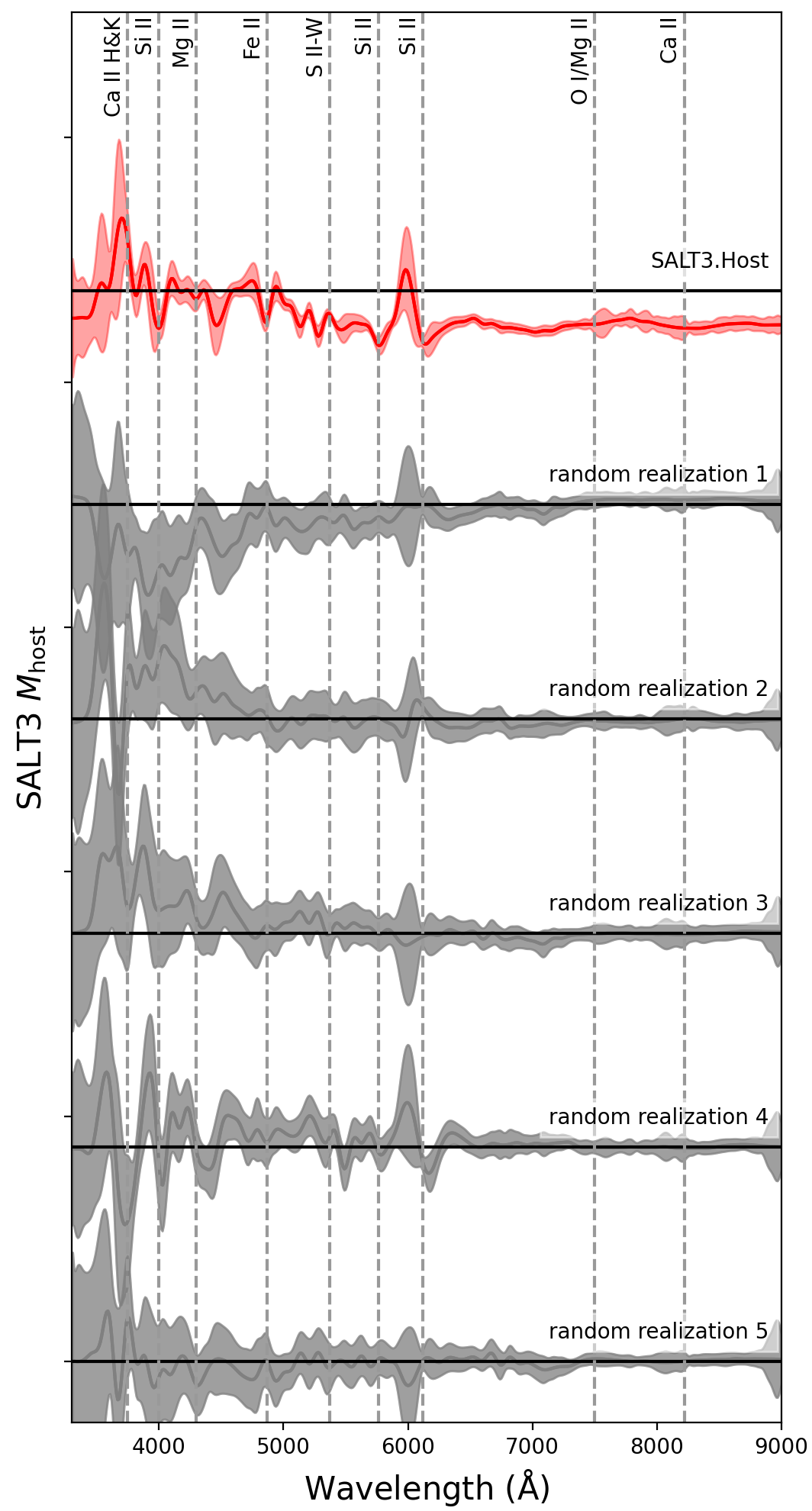
Figure 13: The trained SALT3.Host model at maximum light (red) compared to five models trained when host-galaxy masses are assigned to each SN at random (gray). The models using randomly assigned masses have larger errors, indicating greater variance within the 50 bootstrapping iterations, and all fluctuations are consistent with zero at the 2-$\sigma$ level.

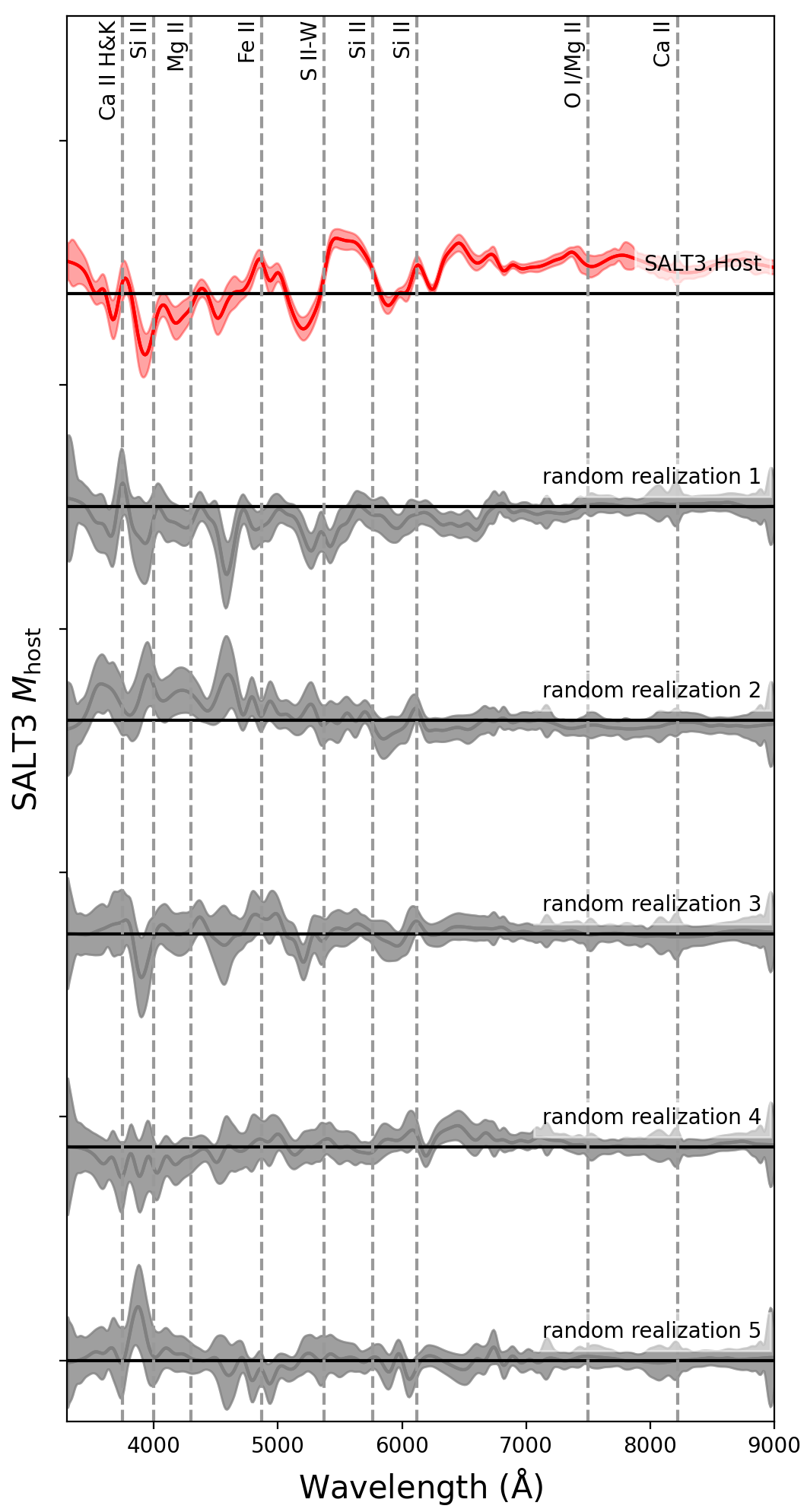
Figure 14: Same as Figure 13 but at phase $+$15 days.

To verify that the recovered, host-mass-dependent spectral features are not due to systematic errors in the SALTshaker training, we train five SALT3.Host models using randomly assigned host-galaxy mass parameters. The results for maximum-light spectra are shown in Figures 13 and 14. We find that the errors on these random models are significantly larger, resulting from greater variance in the 50 bootstrap iterations for each “random” model. We do not recover any spectral features at more than 2-$\sigma$ significance, including at both earlier and later light-curve phases. We do see hints that that some low-significance absorption features may be correlated, e.g., Si II and Ca H&K in random realization 4 at maximum light, due to their correlation in the individual input spectra. There could also be slight hints of wavelength-dependent slopes in some realizations but they are much less significant than the slope seen in the SALT3.Host model.

We also measure the difference in equivalent widths between mean high- and low-mass-hosted SN spectra of the Ca H&K and Si II (6355Å) features for each of the five random realizations. Out of 10 total measurements, four have $>$1-$\sigma$ significance, and one of those four is significant at $>$2$\sigma$. This is consistent with the statistical expectation; for 10 samples in which the errors are due to random noise, one would expect an average of three 1-$\sigma$ outliers and 0.5 2-$\sigma$ outliers.

References

- Abbott et al. (2019) Abbott, T. M. C., Allam, S., Andersen, P., et al. 2019, ApJ, 872, L30, doi: 10.3847/2041-8213/ab04fa
- Barbary et al. (2022) Barbary, K., Bailey, S., Barentsen, G., et al. 2022, SNCosmo, v2.8.0, Zenodo, Zenodo, doi: 10.5281/zenodo.592747
- Bellm et al. (2019) Bellm, E. C., Kulkarni, S. R., Graham, M. J., et al. 2019, PASP, 131, 018002, doi: 10.1088/1538-3873/aaecbe
- Bertin & Arnouts (1996) Bertin, E., & Arnouts, S. 1996, A&AS, 117, 393, doi: 10.1051/aas:1996164
- Betoule et al. (2014) Betoule, M., Kessler, R., Guy, J., et al. 2014, A&A, 568, A22, doi: 10.1051/0004-6361/201423413
- Bohlin et al. (2020) Bohlin, R. C., Hubeny, I., & Rauch, T. 2020, AJ, 160, 21, doi: 10.3847/1538-3881/ab94b4
- Boone et al. (2021a) Boone, K., Aldering, G., Antilogus, P., et al. 2021a, ApJ, 912, 70, doi: 10.3847/1538-4357/abec3c
- Boone et al. (2021b) —. 2021b, ApJ, 912, 71, doi: 10.3847/1538-4357/abec3b
- Branch et al. (1996) Branch, D., Romanishin, W., & Baron, E. 1996, ApJ, 465, 73, doi: 10.1086/177402
- Brout & Scolnic (2021) Brout, D., & Scolnic, D. 2021, ApJ, 909, 26, doi: 10.3847/1538-4357/abd69b
- Brout et al. (2019) Brout, D., Scolnic, D., Kessler, R., et al. 2019, ApJ, 874, 150, doi: 10.3847/1538-4357/ab08a0
- Brout et al. (2021) Brout, D., Taylor, G., Scolnic, D., et al. 2021, arXiv e-prints, arXiv:2112.03864. https://arxiv.org/abs/2112.03864
- Brout et al. (2022) Brout, D., Scolnic, D., Popovic, B., et al. 2022, arXiv e-prints, arXiv:2202.04077. https://arxiv.org/abs/2202.04077
- Bruzual & Charlot (2003) Bruzual, G., & Charlot, S. 2003, MNRAS, 344, 1000, doi: 10.1046/j.1365-8711.2003.06897.x
- Chabrier (2003) Chabrier, G. 2003, PASP, 115, 763, doi: 10.1086/376392
- Chambers et al. (2016) Chambers, K. C., Magnier, E. A., Metcalfe, N., et al. 2016, ArXiv e-prints. https://arxiv.org/abs/1612.05560
- Childress et al. (2013) Childress, M., Aldering, G., Antilogus, P., et al. 2013, ApJ, 770, 108, doi: 10.1088/0004-637X/770/2/108
- Childress et al. (2014) Childress, M. J., Wolf, C., & Zahid, H. J. 2014, MNRAS, 445, 1898, doi: 10.1093/mnras/stu1892
- Dai et al. (2022) Dai, M., Jones, D. O., Kenworthy, W. D., et al. 2022, arXiv e-prints, arXiv:2212.06879, doi: 10.48550/arXiv.2212.06879
- Fakhouri et al. (2015) Fakhouri, H. K., Boone, K., Aldering, G., et al. 2015, ApJ, 815, 58, doi: 10.1088/0004-637X/815/1/58
- Flewelling et al. (2020) Flewelling, H. A., Magnier, E. A., Chambers, K. C., et al. 2020, ApJS, 251, 7, doi: 10.3847/1538-4365/abb82d
- Foley (2013) Foley, R. J. 2013, MNRAS, 435, 273, doi: 10.1093/mnras/stt1292
- Foley & Kasen (2011) Foley, R. J., & Kasen, D. 2011, ApJ, 729, 55, doi: 10.1088/0004-637X/729/1/55
- Foley et al. (2012) Foley, R. J., Filippenko, A. V., Kessler, R., et al. 2012, AJ, 143, 113, doi: 10.1088/0004-6256/143/5/113
- Foley et al. (2018) Foley, R. J., Scolnic, D., Rest, A., et al. 2018, MNRAS, 475, 193, doi: 10.1093/mnras/stx3136
- Gagliano et al. (2021) Gagliano, A., Narayan, G., Engel, A., Carrasco Kind, M., & LSST Dark Energy Science Collaboration. 2021, ApJ, 908, 170, doi: 10.3847/1538-4357/abd02b
- Gallagher et al. (2005) Gallagher, J. S., Garnavich, P. M., Berlind, P., et al. 2005, ApJ, 634, 210, doi: 10.1086/491664
- González-Gaitán et al. (2021) González-Gaitán, S., de Jaeger, T., Galbany, L., et al. 2021, MNRAS, 508, 4656, doi: 10.1093/mnras/stab2802
- Gupta et al. (2016) Gupta, R. R., Kuhlmann, S., Kovacs, E., et al. 2016, AJ, 152, 154, doi: 10.3847/0004-6256/152/6/154
- Guy et al. (2007) Guy, J., Astier, P., Baumont, S., et al. 2007, A&A, 466, 11, doi: 10.1051/0004-6361:20066930
- Guy et al. (2010) Guy, J., Sullivan, M., Conley, A., et al. 2010, A&A, 523, A7, doi: 10.1051/0004-6361/201014468
- Hamuy et al. (2021) Hamuy, M., Cartier, R., Contreras, C., & Suntzeff, N. B. 2021, MNRAS, 500, 1095, doi: 10.1093/mnras/staa3350
- Hamuy et al. (1995) Hamuy, M., Phillips, M. M., Maza, J., et al. 1995, AJ, 109, 1, doi: 10.1086/117251
- Hamuy et al. (1996) Hamuy, M., Phillips, M. M., Suntzeff, N. B., et al. 1996, AJ, 112, 2398, doi: 10.1086/118191
- Hamuy et al. (2000) Hamuy, M., Trager, S. C., Pinto, P. A., et al. 2000, AJ, 120, 1479, doi: 10.1086/301527
- Hayden et al. (2013) Hayden, B. T., Gupta, R. R., Garnavich, P. M., et al. 2013, ApJ, 764, 191, doi: 10.1088/0004-637X/764/2/191
- Hicken et al. (2009) Hicken, M., Challis, P., Jha, S., et al. 2009, ApJ, 700, 331, doi: 10.1088/0004-637X/700/1/331
- Hicken et al. (2012) Hicken, M., Challis, P., Kirshner, R. P., et al. 2012, ApJS, 200, 12, doi: 10.1088/0067-0049/200/2/12
- Howell (2001) Howell, D. A. 2001, ApJ, 554, L193, doi: 10.1086/321702
- Ilbert et al. (2006) Ilbert, O., Arnouts, S., McCracken, H. J., et al. 2006, A&A, 457, 841, doi: 10.1051/0004-6361:20065138
- Jha et al. (2007) Jha, S., Riess, A. G., & Kirshner, R. P. 2007, ApJ, 659, 122, doi: 10.1086/512054
- Jha et al. (2006) Jha, S., Kirshner, R. P., Challis, P., et al. 2006, AJ, 131, 527, doi: 10.1086/497989
- Johansson et al. (2021) Johansson, J., Cenko, S. B., Fox, O. D., et al. 2021, ApJ, 923, 237, doi: 10.3847/1538-4357/ac2f9e
- Jones et al. (2015) Jones, D. O., Scolnic, D. M., & Rodney, S. A. 2015, PythonPhot: Simple DAOPHOT-type photometry in Python, Astrophysics Source Code Library. http://ascl.net/1501.010
- Jones et al. (2013) Jones, D. O., Rodney, S. A., Riess, A. G., et al. 2013, ApJ, 768, 166, doi: 10.1088/0004-637X/768/2/166
- Jones et al. (2018) Jones, D. O., Scolnic, D. M., Riess, A. G., et al. 2018, ApJ, 857, 51, doi: 10.3847/1538-4357/aab6b1
- Jones et al. (2019) Jones, D. O., Scolnic, D. M., Foley, R. J., et al. 2019, ApJ, 881, 19, doi: 10.3847/1538-4357/ab2bec
- Jones et al. (2021) Jones, D. O., Foley, R. J., Narayan, G., et al. 2021, ApJ, 908, 143, doi: 10.3847/1538-4357/abd7f5
- Jones et al. (2022) Jones, D. O., Mandel, K. S., Kirshner, R. P., et al. 2022, arXiv e-prints, arXiv:2201.07801. https://arxiv.org/abs/2201.07801
- Kasen (2006) Kasen, D. 2006, ApJ, 649, 939, doi: 10.1086/506588
- Kelly et al. (2010) Kelly, P. L., Hicken, M., Burke, D. L., Mandel, K. S., & Kirshner, R. P. 2010, ApJ, 715, 743, doi: 10.1088/0004-637X/715/2/743
- Kelsey et al. (2021) Kelsey, L., Sullivan, M., Smith, M., et al. 2021, MNRAS, 501, 4861, doi: 10.1093/mnras/staa3924
- Kelsey et al. (2022) Kelsey, L., Sullivan, M., Wiseman, P., et al. 2022, arXiv e-prints, arXiv:2208.01357. https://arxiv.org/abs/2208.01357
- Kenworthy et al. (2021) Kenworthy, W. D., Jones, D. O., Dai, M., et al. 2021, arXiv e-prints, arXiv:2104.07795. https://arxiv.org/abs/2104.07795
- Kessler et al. (2010) Kessler, R., Bassett, B., Belov, P., et al. 2010, PASP, 122, 1415, doi: 10.1086/657607
- Kim et al. (2018) Kim, Y.-L., Smith, M., Sullivan, M., & Lee, Y.-W. 2018, ApJ, 854, 24, doi: 10.3847/1538-4357/aaa127
- Krisciunas et al. (2017) Krisciunas, K., Contreras, C., Burns, C. R., et al. 2017, AJ, 154, 211, doi: 10.3847/1538-3881/aa8df0
- Lampeitl et al. (2010) Lampeitl, H., Smith, M., Nichol, R. C., et al. 2010, ApJ, 722, 566, doi: 10.1088/0004-637X/722/1/566
- Léget et al. (2020) Léget, P. F., Gangler, E., Mondon, F., et al. 2020, A&A, 636, A46, doi: 10.1051/0004-6361/201834954
- Lu et al. (2022) Lu, J., Hsiao, E. Y., Phillips, M. M., et al. 2022, arXiv e-prints, arXiv:2211.05998, doi: 10.48550/arXiv.2211.05998
- Mandel et al. (2022) Mandel, K. S., Thorp, S., Narayan, G., Friedman, A. S., & Avelino, A. 2022, MNRAS, 510, 3939, doi: 10.1093/mnras/stab3496
- Marriner et al. (2011) Marriner, J., Bernstein, J. P., Kessler, R., et al. 2011, ApJ, 740, 72, doi: 10.1088/0004-637X/740/2/72
- Martin et al. (2005) Martin, D. C., Fanson, J., Schiminovich, D., et al. 2005, ApJ, 619, L1, doi: 10.1086/426387
- Meldorf et al. (2022) Meldorf, C., Palmese, A., Brout, D., et al. 2022, arXiv e-prints, arXiv:2206.06928. https://arxiv.org/abs/2206.06928
- Paulino-Afonso et al. (2022) Paulino-Afonso, A., González-Gaitán, S., Galbany, L., et al. 2022, arXiv e-prints, arXiv:2202.04078. https://arxiv.org/abs/2202.04078
- Phillips (1993) Phillips, M. M. 1993, ApJ, 413, L105, doi: 10.1086/186970
- Pierel et al. (2021) Pierel, J. D. R., Jones, D. O., Dai, M., et al. 2021, ApJ, 911, 96, doi: 10.3847/1538-4357/abe867
- Pierel et al. (2022) Pierel, J. D. R., Jones, D. O., Kenworthy, W. D., et al. 2022, ApJ, 939, 11, doi: 10.3847/1538-4357/ac93f9
- Planck Collaboration et al. (2018) Planck Collaboration, Aghanim, N., Akrami, Y., et al. 2018, ArXiv e-prints. https://arxiv.org/abs/1807.06209
- Ponder et al. (2021) Ponder, K. A., Wood-Vasey, W. M., Weyant, A., et al. 2021, ApJ, 923, 197, doi: 10.3847/1538-4357/ac2d99
- Popovic et al. (2021) Popovic, B., Brout, D., Kessler, R., & Scolnic, D. 2021, arXiv e-prints, arXiv:2112.04456. https://arxiv.org/abs/2112.04456
- Riess et al. (1999) Riess, A. G., Kirshner, R. P., Schmidt, B. P., et al. 1999, AJ, 117, 707, doi: 10.1086/300738
- Riess et al. (2021) Riess, A. G., Yuan, W., Macri, L. M., et al. 2021, arXiv e-prints, arXiv:2112.04510. https://arxiv.org/abs/2112.04510
- Rigault et al. (2013) Rigault, M., Copin, Y., Aldering, G., et al. 2013, A&A, 560, A66, doi: 10.1051/0004-6361/201322104
- Rigault et al. (2015) Rigault, M., Aldering, G., Kowalski, M., et al. 2015, ApJ, 802, 20, doi: 10.1088/0004-637X/802/1/20
- Rigault et al. (2020) Rigault, M., Brinnel, V., Aldering, G., et al. 2020, A&A, 644, A176, doi: 10.1051/0004-6361/201730404
- Rodney et al. (2014) Rodney, S. A., Riess, A. G., Strolger, L.-G., et al. 2014, AJ, 148, 13, doi: 10.1088/0004-6256/148/1/13
- Roman et al. (2018) Roman, M., Hardin, D., Betoule, M., et al. 2018, A&A, 615, A68, doi: 10.1051/0004-6361/201731425
- Rose et al. (2019) Rose, B. M., Garnavich, P. M., & Berg, M. A. 2019, arXiv e-prints. https://arxiv.org/abs/1902.01433
- Rose et al. (2022) Rose, B. M., Popovic, B., Scolnic, D., & Brout, D. 2022, arXiv e-prints, arXiv:2206.09950. https://arxiv.org/abs/2206.09950
- Rose et al. (2021) Rose, B. M., Rubin, D., Strolger, L., & Garnavich, P. M. 2021, ApJ, 909, 28, doi: 10.3847/1538-4357/abd550
- Rose et al. (2020) Rose, B. M., Dixon, S., Rubin, D., et al. 2020, ApJ, 890, 60, doi: 10.3847/1538-4357/ab698d
- Rubin (2020) Rubin, D. 2020, ApJ, 897, 40, doi: 10.3847/1538-4357/ab12de
- Rubin et al. (2013) Rubin, D., Knop, R. A., Rykoff, E., et al. 2013, ApJ, 763, 35, doi: 10.1088/0004-637X/763/1/35
- Saunders et al. (2018) Saunders, C., Aldering, G., Antilogus, P., et al. 2018, ApJ, 869, 167, doi: 10.3847/1538-4357/aaec7e
- Scolnic et al. (2015) Scolnic, D., Casertano, S., Riess, A., et al. 2015, ApJ, 815, 117, doi: 10.1088/0004-637X/815/2/117
- Scolnic et al. (2018) Scolnic, D. M., Jones, D. O., Rest, A., et al. 2018, ApJ, 859, 101, doi: 10.3847/1538-4357/aab9bb
- Siebert et al. (2020) Siebert, M. R., Foley, R. J., Jones, D. O., & Davis, K. W. 2020, MNRAS, 493, 5713, doi: 10.1093/mnras/staa577
- Siebert et al. (2019) Siebert, M. R., Foley, R. J., Jones, D. O., et al. 2019, MNRAS, 486, 5785, doi: 10.1093/mnras/stz1209
- Skrutskie et al. (2006) Skrutskie, M. F., Cutri, R. M., Stiening, R., et al. 2006, AJ, 131, 1163, doi: 10.1086/498708
- Sullivan et al. (2006) Sullivan, M., Le Borgne, D., Pritchet, C. J., et al. 2006, ApJ, 648, 868, doi: 10.1086/506137
- Sullivan et al. (2010) Sullivan, M., Conley, A., Howell, D. A., et al. 2010, MNRAS, 406, 782, doi: 10.1111/j.1365-2966.2010.16731.x
- Taylor et al. (2021) Taylor, G., Lidman, C., Tucker, B. E., et al. 2021, MNRAS, 504, 4111, doi: 10.1093/mnras/stab962
- Taylor et al. (2023) Taylor, G., Jones, D. O., Popovic, B., et al. 2023, MNRAS, 520, 5209, doi: 10.1093/mnras/stad320
- The LSST Dark Energy Science Collaboration et al. (2018) The LSST Dark Energy Science Collaboration, Mandelbaum, R., Eifler, T., et al. 2018, arXiv e-prints, arXiv:1809.01669. https://arxiv.org/abs/1809.01669
- Thorp et al. (2021) Thorp, S., Mandel, K. S., Jones, D. O., Ward, S. M., & Narayan, G. 2021, MNRAS, 508, 4310, doi: 10.1093/mnras/stab2849
- Tripp (1998) Tripp, R. 1998, A&A, 331, 815
- Uddin et al. (2020) Uddin, S. A., Burns, C. R., Phillips, M. M., et al. 2020, ApJ, 901, 143, doi: 10.3847/1538-4357/abafb7
- Wang et al. (2009) Wang, X., Filippenko, A. V., Ganeshalingam, M., et al. 2009, ApJ, 699, L139, doi: 10.1088/0004-637X/699/2/L139
- Wiseman et al. (2022) Wiseman, P., Vincenzi, M., Sullivan, M., et al. 2022, arXiv e-prints, arXiv:2207.05583. https://arxiv.org/abs/2207.05583
- York et al. (2000) York, D. G., Adelman, J., Anderson, John E., J., et al. 2000, AJ, 120, 1579, doi: 10.1086/301513
- Zhao et al. (2015) Zhao, X., Wang, X., Maeda, K., et al. 2015, ApJS, 220, 20, doi: 10.1088/0067-0049/220/1/20