The Mori-Zwanzig formulation of deep learning

Abstract

We develop a new formulation of deep learning based on the Mori-Zwanzig (MZ) formalism of irreversible statistical mechanics. The new formulation is built upon the well-known duality between deep neural networks and discrete dynamical systems, and it allows us to directly propagate quantities of interest (conditional expectations and probability density functions) forward and backward through the network by means of exact linear operator equations. Such new equations can be used as a starting point to develop new effective parameterizations of deep neural networks, and provide a new framework to study deep-learning via operator theoretic methods. The proposed MZ formulation of deep learning naturally introduces a new concept, i.e., the memory of the neural network, which plays a fundamental role in low-dimensional modeling and parameterization. By using the theory of contraction mappings, we develop sufficient conditions for the memory of the neural network to decay with the number of layers. This allows us to rigorously transform deep networks into shallow ones, e.g., by reducing the number of neurons per layer (using projection operators), or by reducing the total number of layers (using the decay property of the memory operator).

1 Introduction

It has been recently shown that new insights on deep learning can be obtained by regarding the process of training a deep neural network as a discretization of an optimal control problem involving nonlinear differential equations [16, 15, 20]. One attractive feature of this formulation is that it allows us to use tools from dynamical system theory such as the Pontryagin maximum principle or the Hamilton-Jacobi-Bellman equation to study deep learning from a rigorous mathematical perspective [33, 21, 37]. For instance, it has been recently shown that by idealizing deep residual networks as continuous-time dynamical systems it is possible to derive sufficient conditions for universal approximation in $L^{p}$, which can also be understood as an approximation theory that leverages flow maps generated by dynamical systems [34].

In the spirit of modeling a deep neural network as a flow of a discrete dynamical system, in this paper we develop a new formulation of deep learning based on the Mori-Zwanzig (MZ) formalism. The MZ formalism was originally developed in statistical mechanics [41, 64] to formally integrate under-resolved phase variables in nonlinear dynamical systems by means of a projection operator. One of the main features of such formulation is that it allows us to systematically derive exact evolution equations for quantities of interest, e.g., macroscopic observables, based on microscopic equations of motion [9, 23, 25, 7, 5, 55, 14, 61, 62].

In the context of deep learning, the MZ formalism can be used to reduce the total number of degrees of freedom of the neural network, e.g., by reducing the number of neurons per layer (using projection operators), or by transforming deep networks into shallows networks, e.g., by approximating the MZ memory operator. Computing the solution of the MZ equation for deep learning is not an easy task. One of the main challenges is the approximation of the memory term and the fluctuation (noise) term, which encode the interaction between the so-called orthogonal dynamics and the dynamics of the quantity of interest. In the context of neural networks, the orthogonal dynamics is essentially a discrete high-dimensional flow governed by a difference equation that is hard to solve. Despite these difficulties, the MZ equation of deep learning is formally exact, and can be used as a starting point to build useful approximations and parameterizations that target the output function directly. Moreover, it provides a new framework to study deep-learning via operator theoretic approaches. For example, the analysis of the memory term in the MZ formulation may shed light on the behaviour of recent neural network architectures such as the long short-term memory (LSTM) network [51, 19].

This paper is organized as follows. In section 2 we briefly review the formulation of deep learning as a control problem involving a discrete stochastic dynamical system. In section 3 we introduce the composition and transfer operators associated with the neural network. Such operators are the discrete analogues of the stochastic Koopman [54, 63] and Frobenius-Perron operators in classical continuous-time nonlinear dynamics. In the neural network setting the composition and transfer operators are integral operators with kernel given by the conditional transition density between one layer and the next. In section 4 we discuss different training paradigms for stochastic neural networks, i.e., the classical “training over weights” paradigm, and a novel “training over noise” paradigm. Training over noise can be seen as an instance of transfer learning in which we optimize for the PDF of the noise to re-purpose a previously trained neural network to another task, without changing the neural network weights and biases. In section 5.3 we present the MZ formulation of deep learning and derive the operator equations at the basis of our theory. In section 6 we introduce a particular class of projection operators, i.e., Mori’s projections [62] and study their properties. In section 7 we develop the analysis of the MZ equation, and derive sufficient conditions under which the MZ memory term decays with the number of layers. This allows us to approximate the MZ memory term with just a few terms and re-parameterize the network accordingly. The main findings are summarized in section 8. We also include two appendices in which we establish theoretical results concerning the composition and transfer operators for neural networks with additive random perturbations, and prove the Markovian property of neural networks driven by discrete random processes characterized by statistically independent random vectors.

2 Modeling neural networks as discrete stochastic dynamical systems

We model a neural network with $L$ layers as a discrete stochastic dynamical system of the form

$$\bm{X}_{n+1}=\bm{H}_{n}(\bm{X}_{n},\bm{w}_{n},\bm{\xi}_{n}),\qquad{n=0,1,\cdots,L-1}.$$ (1)

Here, the index $n$ labels a specific layer in the network, $\bm{H}_{n}$ is the transition function of the $(n+1)$ layer, $\bm{X}_{0}\in\mathbb{R}^{d}$ is the network input, $\bm{X}_{n}\in\mathbb{R}^{d_{n}}$ is the output of the $n$-th layer, $\{\bm{\xi}_{0},\ldots,\bm{\xi}_{L-1}\}$ are random vectors, and $\bm{w}_{n}\in\mathbb{R}^{q_{n}}$ are parameters characterizing the $(n+1)$ layer. We allow the input $\bm{X}_{0}$ to be random. Furthermore, we assume that the random vectors $\{\bm{\xi}_{0},\ldots,\bm{\xi}_{L-1}\}$ are statistically independent, and that $\bm{\xi}_{n}$ is independent of past and current states, i.e., $\{\bm{X}_{0},\ldots,\bm{X}_{n}\}$. In this assumption, the neural network model (1) defines a Markov process $\{\bm{X}_{n}\}$ (see B). Further assumptions about the mapping $\bm{H}_{n}$ and its relation to the noise process will be stated in subsequent sections.

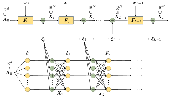
Figure 1: Sketch of a stochastic neural network model of the form (2), with $L$ layers and $N$ neurons per layer. We assume that the random vectors $\{\bm{\xi}_{0},\ldots,\bm{\xi}_{L-1}\}$ are statistically independent, and that $\bm{\xi}_{n}$ is independent of past and current states, i.e., $\{\bm{X}_{0},\ldots,\bm{X}_{n}\}$. With these assumptions, $\{\bm{X}_{0},\ldots,\bm{X}_{L}\}$ is a Markov process (see B).

The general formulation (1) includes the following important classes of neural networks:

1. Neural networks perturbed by additive random noise (Figure 1). These models are of the form

   $$\bm{X}_{n+1}=\bm{F}_{n}(\bm{X}_{n},\bm{w}_{n})+\bm{\xi}_{n},\qquad n=0,\ldots,L-1.$$ (2)

   The mapping $\bm{F}_{n}$ is often defined as a composition of a layer-dependent affine transformation with an activation function $\varphi$, i.e.,

   $$\bm{F}_{n}(\bm{X}_{n},\bm{w}_{n})=\varphi(\bm{W}_{n}\bm{X}_{n}+\bm{b}_{n})\qquad\bm{w}_{n}=\{\bm{W}_{n},\bm{b}_{n}\},$$ (3)

   where $\bm{W}_{n}$ is a $d_{n+1}\times d_{n}$ weight matrix, and $\bm{b}_{n}\in\mathbb{R}^{d_{n+1}}$ is a bias vector.
   

2. Neural networks perturbed by multiplicative random noise (Figure 2). These models are of the form

   $$\bm{X}_{n+1}=\bm{F}_{n}(\bm{X}_{n},\bm{w}_{n})+\bm{M}_{n}(\bm{X}_{n})\bm{\xi}_{n},\qquad n=0,\ldots,L-1,$$ (4)

   where $\bm{M}_{n}(\bm{X}_{n})$ is a matrix depending on $\bm{X}_{n}$.
   

   

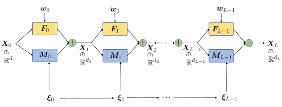
   Figure 2: Sketch of the stochastic neural network model (4). We assume that the random vectors $\{\bm{\xi}_{0},\ldots,\bm{\xi}_{L-1}\}$ are statistically independent, and that $\bm{\xi}_{n}$ is independent of past and current states, i.e., $\{\bm{X}_{0},\ldots,\bm{X}_{n}\}$. In this assumption, the neural network model (4) defines a Markov process $\{\bm{X}_{n}\}$. Note that the dimension of the vectors $\bm{X}_{n}$ can vary from layer to layer, e.g., in encoding or decoding neural networks.

3. Neural networks with random weights and biases [18, 58]. These models are of the form

   $$\bm{X}_{n+1}=\varphi\left({\bm{Z}}_{n}\bm{X}_{n}+{\bm{z}}_{n}\right),\qquad n=0,\ldots,L-1$$ (5)

   where ${\bm{Z}}_{n}$ are random weight matrices, and ${\bm{z}}_{n}$ are random bias vectors. The pairs $\{{\bm{Z}}_{n},{\bm{z}}_{n}\}$ and $\{{\bm{Z}}_{j},{\bm{z}}_{j}\}$ are assumed to be statistically independent for $n\neq j$. Moreover, $\{{\bm{Z}}_{j},{\bm{z}}_{j}\}$ are independent of the neural network states $\{\bm{X}_{0},\ldots,\bm{X}_{j}\}$ for all $j=0,\ldots,L-1$.

In this article, we will focus our attention primarily on neural network models with additive random noise, i.e., models of the form (2). The functional setting for these models is extensively discussed in A. The neural network output is usually written as

$$q_{L}(\bm{x})=\bm{\alpha}\cdot\mathbb{E}\left[\bm{X}_{L}|\bm{X}_{0}=\bm{x}\right],$$ (6)

where $\bm{\alpha}$ is a vector of output weights, and $\mathbb{E}\left[\bm{X}_{L}|\bm{X}_{0}=\bm{x}\right]$ is the expectation of the random vector $\bm{X}_{L}$ conditional to $\bm{X}_{0}=\bm{x}$. In the absence of noise, (6) reduces to the well-known function composition rule

$$q_{L}(\bm{x})=\bm{\alpha}\cdot\bm{F}_{L-1}(\bm{F}_{L-2}(\cdots\bm{F}_{1}(\bm{F}_{0}(\bm{x},\bm{w}_{0}),\bm{w}_{1}),\cdots,\bm{w}_{L-2}),\bm{w}_{L-1}).$$ (7)

The neural network parameters $\{\bm{\alpha},\bm{w}_{0},\ldots,\bm{w}_{L-1}\}$ appearing in (6) or (7) are usually determined by minimizing a dissimilarity measure between $q_{L}(\bm{x})$ and a given target function $f(\bm{x})$ (supervised learning). By adding random noise to the neural network, e.g., in the form of additive noise or by randomizing weights and biases, we are essentially adding an infinite number of degrees of freedom to the system, which can be leveraged for training and transfer learning (see section 4).

3 Composition and transfer operators for neural networks

In this section we derive the composition and transfer operators associated with the neural network model (1), which map, respectively, the conditional expectation $\mathbb{E}\left\{\bm{u}(\bm{X}_{L})|\bm{X}_{n}=\bm{x}\right\}$ (where $\bm{u}(\cdot)$ is a user-defined measurable function) and $p_{n}(\bm{x})$ (the probability density of $\bm{X}_{n}$) forward and backward across the network. To this end, we assume that the random vectors $\{\bm{\xi}_{0},\ldots,\bm{\xi}_{L-1}\}$ in (1) are statistically independent, and that $\bm{\xi}_{n}$ is independent of past and current states, i.e., $\{\bm{X}_{0},\ldots,\bm{X}_{n}\}$, With these assumptions, $\{\bm{X}_{n}\}$ in (1) is a discrete Markov process (see B). Hence, the joint probability density function (PDF) of the random vectors $\{\bm{X}_{0},\ldots,\bm{X}_{L}\}$, i.e., joint PDF of the state of the entire neural network, can be factored as

$$p(\bm{x}_{0},\ldots,\bm{x}_{L})=p_{L|L-1}(\bm{x}_{L}|\bm{x}_{L-1})p_{L-1|L-2}(\bm{x}_{L-1}|\bm{x}_{L-2})\cdots p_{1|0}(\bm{x}_{1}|\bm{x}_{0})p_{0}(\bm{x}_{0}).$$ (8)

By using the identity (Bayes’ theorem)

$$p(\bm{x}_{k+1},\bm{x}_{k})=p_{k+1|k}(\bm{x}_{k+1}|\bm{x}_{k})p_{k}(\bm{x}_{k})=p_{k|k+1}(\bm{x}_{k}|\bm{x}_{k+1})p_{k+1}(\bm{x}_{k+1})$$ (9)

we see that the chain of transition probabilities (8) can be reverted, yielding

$$p(\bm{x}_{0},\ldots,\bm{x}_{L})=p_{0|1}(\bm{x}_{0}|\bm{x}_{1})p_{1|2}(\bm{x}_{1}|\bm{x}_{2})\cdots p_{L-1|L}(\bm{x}_{L-1}|\bm{x}_{L})p_{L}(\bm{x}_{L}).$$ (10)

From these expressions, it follows that

$$p_{n|q}(\bm{x}|\bm{y})=\int p_{n|j}(\bm{x}|\bm{z})p_{j|q}(\bm{z}|\bm{y})d\bm{z},$$ (11)

for all indices $n$, $j$ and $q$ in $\{0,\ldots,L\}$, excluding $n=j=q$. The transition probability equation (11) is known as discrete Chapman-Kolmogorov equation and it allows us to define the transfer operator mapping the PDF $p_{n}(\bm{x}_{n})$ into $p_{n+1}(\bm{x}_{n+1})$, together with the composition operator for the conditional expectation $\mathbb{E}\{\bm{u}(\bm{x}_{L})|\bm{X}_{n}=\bm{x}_{n}\}$. As we shall see hereafter, the discrete composition and transfer operators are adjoint to one another.

3.1 Transfer operator

Let us denote by $p_{q}(\bm{x})$ the PDF of $\bm{X}_{q}$, i.e., the output of the $q$-th neural network layer. We first define the operator that maps $p_{q}(\bm{x})$ into $p_{n}(\bm{x})$. By integrating the joint probability density of $\bm{X}_{n}$ and $\bm{X}_{q}$, i.e., $p_{n|q}(\bm{x}|\bm{y})p_{q}(\bm{y})$ with respect to $\bm{y}$ we immediately obtain

$$p_{n}(\bm{x})=\int p_{n|q}(\bm{x}|\bm{y})p_{q}(\bm{y})d\bm{y}.$$ (12)

At this point, it is convenient to define the linear operator

$$\mathcal{N}(n,q)f(\bm{x})=\int p_{n|q}(\bm{x}|\bm{y})f(\bm{y})d\bm{y}.$$ (13)

$\mathcal{N}(n,q)$ is known as transfer (or Frobenius-Perron) operator [14]. From a mathematical viewpoint $\mathcal{N}(n,q)$ is a integral operator with kernel $p_{n|q}(\bm{x},\bm{y})$, i.e., the transition density integrated “from the right”. It follows from the Chapman-Kolmogorov identity (11) that the set of integral operators $\{\mathcal{N}(n,q)\}$ satisfies

$$\mathcal{N}(n,q)=\mathcal{N}(n,j)\mathcal{N}(j,q),\qquad\mathcal{N}(j,j)=\mathcal{I},\qquad\forall n,j,q\in\{0,\ldots,L\},$$ (14)

where $\mathcal{I}$ is the identity operator. The operator $\mathcal{N}$ allows us to map the one-layer PDF, e.g., the PDF of $\bm{X}_{q}$, either forward or backward across the neural network (see Figure 3). As an example, consider a network with four layers and states $\bm{X}_{0}$ (input), $\bm{X}_{1}$, $\bm{X}_{2}$, $\bm{X}_{3}$, and $\bm{X}_{4}$ (output). Then Eq. (13) implies that,

$$p_{2}(\bm{x})=\underbrace{\mathcal{N}(2,1)\mathcal{N}(1,0)}_{\mathcal{N}(2,0)}p_{0}(\bm{x})=\underbrace{\mathcal{N}(2,3)\mathcal{N}(3,4)}_{\mathcal{N}(2,4)}p_{4}(\bm{x}).$$

In summary, we have

$$p_{n}(\bm{x})=\mathcal{N}(n,q)p_{q}(\bm{x})\qquad\forall n,q\in\{0,\ldots,L\},$$ (15)

where

$$\mathcal{N}(n,q)p_{q}(\bm{x})=\int p_{n|q}(\bm{x}|\bm{y})p_{q}(\bm{y})d\bm{y}.$$ (16)

We emphasize that modeling the PDF dynamics via neural networks has been studied extensively in machine learning, e.g., in the theory of normalizing flows for density estimation or variational inference [49, 30, 52].

3.2 Composition operator

For any measurable deterministic function $\bm{u}(\bm{x})$, the expectation of $\bm{u}(\bm{X}_{j})$ conditional to $\bm{X}_{n}=\bm{x}$ is defined as

$$\mathbb{E}\left\{\bm{u}(\bm{X}_{j})|\bm{X}_{n}=\bm{x}\right\}=\int\bm{u}(\bm{y})p_{j|n}(\bm{y}|\bm{x})d\bm{y}.$$ (17)

A substitution of (11) into (17) yields

$$\mathbb{E}\left\{\bm{u}(\bm{X}_{j})|\bm{X}_{n}=\bm{x}\right\}=\int\mathbb{E}\left\{\bm{u}(\bm{X}_{j})|\bm{X}_{q}=\bm{y}\right\}p_{q|n}(\bm{y}|\bm{x})d\bm{y},$$ (18)

which holds for all $j,n,q\in\{0,\ldots,L-1\}$. At this point, it is convenient to define the integral operator

$$\mathcal{M}(n,q)f(\bm{x})=\int f(\bm{y})p_{q|n}(\bm{y}|\bm{x})d\bm{y},$$ (19)

which is known as composition [14] or “stochastic Koopman” [54, 63] operator. The operator (19) is also related to the Kolmogorov backward equation [47] . Thanks to the Chapman-Kolmogorov identity (11), the operators $\mathcal{M}(q,j)$ satisfy

$$\mathcal{M}(n,q)=\mathcal{M}(n,j)\mathcal{M}(j,q),\qquad\mathcal{M}(j,j)=\mathcal{I},\qquad\forall n,j,q\in\{0,\ldots,L\},$$ (20)

where $\mathcal{I}$ is the identity operator. Equation (20) allows us to map the conditional expectation (17) of any measurable phase space function $\bm{u}(\bm{X}_{j})$ forward or backward through the network. As an example, consider again a neural network with four layers and states $\{\bm{X}_{0},\dots,\bm{X}_{4}\}$. We have

$$\mathbb{E}\{\bm{u}(\bm{X}_{j})|\bm{X}_{2}=\bm{x}\}= \mathcal{M}(2,3)\mathcal{M}(3,4)\mathbb{E}\{\bm{u}(\bm{X}_{j})|\bm{X}_{4}=\bm{x}\}$$

$$= \mathcal{M}(2,1)\mathcal{M}(1,0)\mathbb{E}\{\bm{u}(\bm{X}_{j})|\bm{X}_{0}=\bm{x}\}.$$ (21)

Equation (21) holds for every $j\in\{0,..,4\}$. Of particular interest in the machine-learning context is the conditional expectation of $\bm{u}(\bm{X}_{L})$ (network output) given $\bm{X}_{0}=\bm{x}$ (network input), which can be computed as

$$\mathbb{E}\{\bm{u}(\bm{X}_{L})|\bm{X}_{0}=\bm{x}\} =\mathcal{M}(0,L)\bm{u}(\bm{x}),$$

$$=\mathcal{M}(0,1)\mathcal{M}(1,2)\cdots\mathcal{M}(L-1,L)\bm{u}(\bm{x}),$$ (22)

i.e., by propagating $\bm{u}(\bm{x})=\mathbb{E}\{\bm{u}(\bm{X}_{L})|\bm{X}_{L}=\bm{x}\}$ backward through the neural network using single layer operators $\mathcal{M}(i-1,i)$. Similarly, we can compute, e.g., $\mathbb{E}\{\bm{u}(\bm{X}_{0})|\bm{X}_{L}=\bm{x}\}$ as

$$\mathbb{E}\{\bm{u}(\bm{X}_{0})|\bm{X}_{L}=\bm{x}\}=\mathcal{M}(L,0)\bm{u}(\bm{x}).$$ (23)

For subsequent analysis, it is convenient to define

$$\bm{q}_{n}(\bm{x})=\mathbb{E}\{\bm{u}(\bm{X}_{L})|\bm{X}_{L-n}=\bm{x}\}.$$ (24)

In this way, if $\mathbb{E}\{\bm{u}(\bm{X}_{L})|\bm{X}_{n}=\bm{x}\}$ is propagated backward through the network by $\mathcal{M}(n-1,n)$, then $\bm{q}_{n}(x)$ is propagated forward by the operator

$$\mathcal{G}(n,q)= \mathcal{M}(L-n,L-q).$$ (25)

In fact, equations (24)-(25) allow us to write (22) in the equivalent form

$$\bm{q}_{L}(\bm{x})= \mathcal{G}(L,L-1)\bm{q}_{L-1}(\bm{x})$$

$$= \mathcal{G}(L,L-1)\cdots\mathcal{G}(1,0)\bm{q}_{0}(\bm{x}),$$ (26)

i.e., as a forward propagation problem (see Figure 3). Note that we can write (26) (or (22)) explicitly in terms of iterated integrals involving single-layer transition densities as

$$\bm{q}_{L}(\bm{x})= \int\bm{u}(\bm{y})p_{0|L}(\bm{y}|\bm{x})d\bm{y}$$

$$= \int\bm{u}(\bm{y})\left(\int\cdots\int p_{L|L-1}(\bm{y}|\bm{x}_{L-1})\cdots p_{2|1}(\bm{x}_{2}|\bm{x}_{1})p_{1|0}(\bm{x}_{1}|\bm{x})d\bm{x}_{L-1}\cdots d\bm{x}_{1}\right)d\bm{y}.$$ (27)

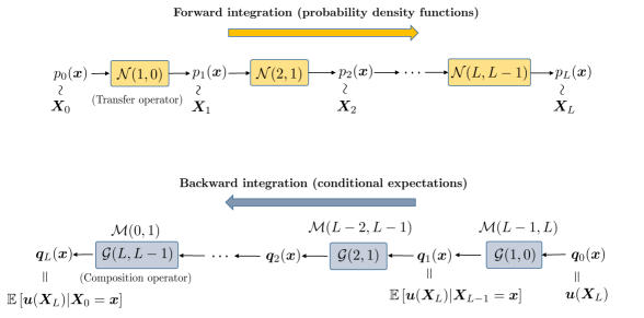
Figure 3: Sketch of the forward/backward integration process for probability density functions (PDFs) and conditional expectations. The transfer operator $\mathcal{N}(n+1,n)$ maps the PDF of $\bm{X}_{n}$ into the PDF of $\bm{X}_{n+1}$ forward through the neural network. On the other hand, the composition operator $\mathcal{M}$ maps the conditional expectation $\mathbb{E}\left[\bm{u}(\bm{X}_{L})|\bm{X}_{n+1}=\bm{x}\right]$ backwards to $\mathbb{E}\left[\bm{u}(\bm{X}_{L})|\bm{X}_{n}=\bm{x}\right]$. By defining the operator $\mathcal{G}(n,m)=\mathcal{M}(L-n,L-m)$ we can transform the backward propagation problem for $\mathbb{E}\left[\bm{u}(\bm{X}_{L})|\bm{X}_{n}=\bm{x}\right]$ into a forward propagation problem for $\bm{q}_{n}(\bm{x})=\mathbb{E}\left[\bm{u}(\bm{X}_{L})|\bm{X}_{L-n}=\bm{x}\right]$.

3.3 Relation between composition and transfer operators

The integral operators $\mathcal{M}$ and $\mathcal{N}$ defined in (19) and (13) involve the same kernel function, i.e., the multi-layer transition density $p_{q|n}(\bm{x},\bm{y})$. In particular, $\mathcal{M}(n,q)$ integrates $p_{q|n}$ “from the left”, while $\mathcal{N}(q,n)$ integrates it “from the right”. It is easy to show that $\mathcal{M}(n,q)$ and $\mathcal{N}(q,n)$ are adjoint to each other relative to the standard inner product in $L^{2}$ (see [14] for the continuous-time case). In fact,

$$\mathbb{E}\{\bm{u}(\bm{X}_{k})\}= \int\mathbb{E}\{\bm{u}(\bm{X}_{k})|\bm{X}_{q}=\bm{x}\}p_{q}(\bm{x})d\bm{x}$$

$$= \int\left[\mathcal{M}(q,j)\mathbb{E}\{\bm{u}(\bm{X}_{k})|\bm{X}_{j}=\bm{x}\}\right]p_{q}(\bm{x})d\bm{x}$$

$$= \int\mathbb{E}\{\bm{u}(\bm{X}_{k})|\bm{X}_{j}=\bm{x}\}\mathcal{N}(j,q)p_{q}(\bm{x})d\bm{x}.$$ (28)

Therefore

$$\mathcal{M}(q,j)^{*}=\mathcal{N}(j,q)\qquad\forall q,j\in\{0,\ldots,L\},$$ (29)

where $\mathcal{M}(q,j)^{*}$ denotes the operator adjoint of $\mathcal{M}(q,j)$ with respect to the $L^{2}$ inner product. By invoking the definition (25), we can also write (29) as

$$\mathcal{G}(L-q,L-j)^{*}=\mathcal{N}(j,q),\qquad\forall j,q\in\{0,\ldots,L\}.$$ (30)

In A we show that if the cumulative distribution function of each random vector $\bm{\xi}_{n}$ in the noise process has partial derivatives that are Lipschitz continuous in $\mathscr{R}(\bm{\xi}_{n})$ (range of $\bm{\xi}_{n}$), then the composition and transfer operators defined in Eqs. (19) and 13 are bounded in $L^{2}$ (see Proposition 16 and Proposition 17). Moreover, is possible to choose the probability density of $\bm{\xi}_{n}$ such that the single layer composition and transfer operators become strict contractions. This property will be used in section 7 to prove that the memory of a stochastic neural network driven by particular types of noise decays with the number of layers.

3.4 Multi-layer conditional transition density

We have seen that the composition and the transfer operators $\mathcal{M}$ and $\mathcal{N}$ defined in Eqs. (19) and (13), allow us to push forward and backward conditional expectations and probability densities across the neural network. Moreover, such operators are adjoint to one another (section 3.3), and also have the same kernel, i.e., the transition density $p_{n|q}(\bm{x}_{n}|\bm{x}_{q})$. In this section, we derive analytical formulas for the one-layer transition density $p_{n+1|n}(\bm{x}_{n+1}|\bm{x}_{n})$ corresponding to the neural network models we discussed in section 2. The multi-layer transition density $p_{n|q}(\bm{x}_{n}|\bm{x}_{q})$ is then obtained by composing one-layer transition densities as follows

$$p_{n|q}(\bm{x}_{n}|\bm{x}_{q})=\int\cdots\int p_{n|n-1}(\bm{x}_{n}|\bm{x}_{n-1})\cdots p_{q+1|q}(\bm{x}_{q+1}|\bm{x}_{q})d\bm{x}_{n-1}\cdots d\bm{x}_{q+1}.$$ (31)

We first consider the general class of stochastic neural network models defined by equation (1). By the definition of conditional probability density, we have

$$p_{n+1|n}(\bm{x}_{n+1}|\bm{x}_{n})=\int p_{\bm{X}_{n+1}|\bm{X}_{n},\bm{\xi}_{n}}(\bm{x}_{n+1}|\bm{x}_{n},\bm{\xi}_{n})p_{\bm{\xi}_{n}|\bm{X}_{n}}(\bm{\xi}_{n}|\bm{x}_{n})d\bm{\xi}_{n}.$$ (32)

By assumption, $p_{\bm{\xi}_{n}|\bm{X}_{n}}(\bm{\xi}_{n}|\bm{x}_{n})=\rho_{n}(\bm{\xi}_{n})$ (the random vector $\bm{\xi}_{n}$ is independent of $\bm{X}_{n}$) and therefore

$$p_{n+1|n}(\bm{x}_{n+1}|\bm{x}_{n})=\int\delta\left(\bm{x}_{n+1}-\bm{H}_{n}\left(\bm{x}_{n},\bm{w}_{n},\bm{\xi}_{n}\right)\right)\rho_{n}(\bm{\xi}_{n})d\bm{\xi}_{n},$$ (33)

where we denoted by $\delta(\cdot)$ the Dirac delta function, and set $\rho_{n}(\bm{\xi}_{n})=p_{\bm{\xi}_{n}}(\bm{\xi}_{n})$. The delta function arises because if $\bm{x}_{n}$ and $\bm{\xi}_{n}$ are known then $\bm{x}_{n+1}$ is obtained by a purely deterministic relationship, i.e, Eq. (1).

The general expression (33) can be simplified for particular classes of stochastic neural network models. For example, if the neural network has purely additive noise as in equation (2), then by using elementary properties of the delta function we obtain

$$p_{n+1|n}(\bm{x}_{n+1}|\bm{x}_{n})= \int\delta\left(\bm{x}_{n+1}-\bm{F}_{n}\left(\bm{x}_{n},\bm{w}_{n}\right)-\bm{\xi}_{n}\right)\rho_{n}(\bm{\xi}_{n})d\bm{\xi}_{n}$$

$$= \rho_{n}\left(\bm{x}_{n+1}-\bm{F}_{n}\left(\bm{x}_{n},\bm{w}_{n}\right)\right).$$ (34)

Note that such transition density depends on the PDF of random vector $\bm{\xi}_{n}$ (i.e., $\rho_{n}$), the one-layer transition function $\bm{F}_{n}$, and the parameters $\bm{w}_{n}$. Similarly, one-layer transition density associated with the stochastic neural network model (4) can be computed by substituting $\bm{H}_{n}(\bm{x}_{n},\bm{w}_{n},\bm{\xi}_{n})=\bm{F}_{n}(\bm{x}_{n},\bm{w}_{n})-\bm{M}_{n}(\bm{x}_{n})\bm{\xi}_{n}$ into (33). This yields

$$p_{n+1|n}(\bm{x}_{n+1}|\bm{x}_{n})=\int\delta\left(\bm{x}_{n+1}-\bm{F}_{n}(\bm{x}_{n},\bm{w}_{n})-\bm{M}_{n}(\bm{x}_{n})\bm{\xi}_{n}\right)\rho_{n}(\bm{\xi}_{n})d\bm{\xi}_{n}.$$ (35)

By using well-known properties of the multivariate delta function [28] it is possible to re-write the integrand in (35) in a more convenient way. For instance, if the matrix $\bm{M}_{n}(\bm{x}_{n})$ has full rank then

$$\delta\left(\bm{x}_{n+1}-\bm{F}_{n}(\bm{x}_{n},\bm{w}_{n})-\bm{M}_{n}(\bm{x}_{n})\bm{\xi}_{n}\right)=\frac{1}{\left|\det(\bm{M}_{n}(\bm{x}_{n}))\right|}\delta\left(\bm{\xi}_{n}-\bm{M}_{n}(\bm{x}_{n})^{-1}\left[\bm{x}_{n+1}-\bm{F}_{n}(\bm{x}_{n},\bm{w}_{n})\right]\right),$$ (36)

which yields

$$p_{n+1|n}(\bm{x}_{n+1}|\bm{x}_{n})=\frac{1}{\left|\det(\bm{M}_{n}(\bm{x}_{n}))\right|}\rho_{n}\left(\bm{M}(\bm{x}_{n})^{-1}\left[\bm{x}_{n+1}-\bm{F}_{n}(\bm{x}_{n},\bm{w}_{n})\right]\right).$$ (37)

Other cases where $\bm{M}_{n}(\bm{x}_{n})$ is not a square matrix can be handled similarly [45, 28]. Finally, consider the neural network model with random weights and biases (5). The one-layer transition density in this case can be expressed as

$$p_{n+1|n}(\bm{x}_{n+1}|\bm{x}_{n})=\int\delta\left(\bm{x}_{n+1}-\varphi\left(\bm{Z}_{n}\bm{x}_{n}+\bm{z}_{n}\right)\right)p(\bm{Z}_{n},\bm{z}_{n})d\bm{Z}_{n}d\bm{z}_{n},$$ (38)

where $p(\bm{Z}_{n},\bm{z}_{n})$ is the joint PDF of the weight matrix and bias vector in the $n$-th layer.

Remark: The transition density (34) associated with the neural network model (2) can be computed explicitly once we choose a probability model for $\bm{\xi}_{n}\in\mathbb{R}^{N}$. For instance, if we assume that $\{\bm{\xi}_{0},\bm{\xi}_{1},\ldots,\bm{\xi}_{L-1}\}$ are i.i.d. Gaussian random vectors with PDF,

$$\rho_{n}(\bm{\xi})=\frac{1}{(2\pi)^{N/2}}e^{-\bm{\xi}\cdot\bm{\xi}/2},\qquad n=0,\ldots,L-1,$$ (39)

then we can explicitly write the one-layer transition density (34) as

$$p_{n+1|n}(\bm{x}_{n+1}|\bm{x}_{n})=\frac{1}{(2\pi)^{N/2}}\exp\left[-\frac{\left[\bm{x}_{n+1}-\bm{F}_{n}(\bm{x}_{\bm{n}},\bm{w}_{n})\right]\cdot\left[\bm{x}_{n+1}-\bm{F}_{n}(\bm{x}_{\bm{n}},\bm{w}_{n})\right]}{2}\right].$$ (40)

In A we provide an analytical example of transition density for a neural network with two layers, one neuron per layer, $\tanh(\cdot)$ activation function, and uniformly distributed random noise.

3.5 The zero noise limit

An important question is what happens to the neural network as we send the amplitude of the noise to zero. To answer this question consider the neural network model (2) with $N$ neurons per layer, and introduce the parameter $\epsilon\geq 0$, i.e.,

$$\bm{X}_{n+1}=\bm{F}_{n}(\bm{X}_{n},\bm{w}_{n})+\epsilon\bm{\xi}_{n},$$ (41)

We are interested in studying the orbits of the discrete dynamical system (41) as $\epsilon\rightarrow 0$. To this end, we assume $\{\bm{\xi}_{n}\}$ independent random vectors with density $\rho_{n}(\bm{x})$. This implies that the PDF of $\epsilon\bm{\xi}_{n}$ is

$$\epsilon\bm{\xi}_{n}\sim\frac{1}{\epsilon^{N}}\rho_{n}\left(\frac{\bm{x}}{\epsilon}\right).$$ (42)

It is shown in [31, Proposition 10.6.1] that the transfer operator $\mathcal{N}(n+1,n)$ associated with (41), i.e.,

$$p_{n+1}(\bm{x})= \mathcal{N}(n+1,n)p_{n}(\bm{x})$$

$$= \int\frac{1}{\epsilon^{N}}\rho_{n}\left(\frac{\bm{x}-\bm{F}_{n}(\bm{z},\bm{w}_{n})}{\epsilon}\right)p_{n}(\bm{z})d\bm{z}$$ (43)

converges in norm to the Frobenius-Perron operator corresponding to $\bm{F}_{n}(\bm{X}_{n},\bm{w}_{n})$ as $\epsilon\rightarrow 0$. Indeed, in the limit $\epsilon\rightarrow 0$ we have, formally

$$\lim_{\epsilon\rightarrow 0}p_{n|n+1}\left(\bm{x}_{n+1}|\bm{x}_{n}\right)=\lim_{\epsilon\rightarrow 0}\int\frac{1}{\epsilon^{N}}\rho_{n}\left(\frac{\bm{x}_{n+1}-\bm{F}_{n}(\bm{x}_{n},\bm{w}_{n})}{\epsilon}\right)=\delta\left(\bm{x}_{n+1}-\bm{F}_{n}(\bm{x}_{n},\bm{w}_{n})\right).$$ (44)

Substituting this expression into (13), one gets,

$$p_{n+1}(\bm{x})=\mathcal{N}(n+1,n)p_{n}(\bm{x})=\int\delta\big{(}\bm{x}-\bm{F}_{n}(\bm{z},\bm{w}_{n})\big{)}p_{n}(\bm{z})d\bm{z}.$$ (45)

Similarly, a substitution into equation (26) yields

$$\bm{q}_{n}(\bm{x})=\mathcal{G}(n,n-1)\bm{q}_{n-1}(\bm{x})=\bm{q}_{n-1}\left(\bm{F}_{L-n}(\bm{x},\bm{w}_{L-n})\right).$$ (46)

Iterating this expression all the way back to $n=1$ yields the familiar function composition rule for neural networks, i.e.,

$$\bm{q}_{L}= \bm{q}_{0}\Big{(}\bm{F}_{L-1}\big{(}\bm{F}_{L-2}(\cdots\bm{F}_{0}(\bm{x},\bm{w}_{0}),\cdots,\bm{w}_{L-2}),\bm{w}_{L-1}\big{)}\Big{)}.$$ (47)

Recalling that $\bm{q}_{0}(\bm{x})=\bm{u}(\bm{x})$ and assuming that $\bm{u}(\bm{x})=\bm{A}\bm{x}$ (linear output layer), where $\bm{A}$ is a matrix of output weights and $\bm{x}$ is a column vector, we can write (47) as

$$\bm{q}_{L}\bm{(}x)= \bm{A}\bm{F}_{L-1}(\bm{F}_{L-2}(\cdots\bm{F}_{1}(\bm{F}_{0}(\bm{x},\bm{w}_{0}),\bm{w}_{1}),\cdots,\bm{w}_{L-2}),\bm{w}_{L-1}).$$ (48)

If $\bm{u}(\bm{x})$ is a linear scalar function, i.e., $u(\bm{x})=\bm{\alpha}\cdot\bm{x}$ then (48) coincides with equation (7).

4 Training paradigms

By adding random noise to a neural network we are essentially adding an infinite number of degrees of freedom to our system. This allows us to rethink the process of training the neural network from a probabilistic perspective. In particular, instead of optimizing a performance metric relative to the neural network weights $\bm{w}=\{\bm{w}_{0},\bm{w}_{1},\ldots,\bm{w}_{L-1}\}$ (classical “training over weights” paradigm), we can now optimize the transition density $p_{n+1|n}(\bm{x}_{n+1}|\bm{x}_{n})$. Clearly, such transition density depends on the neural network weights and on the functional form of the one-layer transition function, e.g., as in equation (34). Hence, if we prescribe the PDF of $\bm{\xi}_{n}$ (e.g., $\rho_{n}$ in (34)), then the transition density $p_{n+1|n}$ is uniquely determined by the functional form of function $\bm{F}_{n}$, and by the weights $\bm{w}_{n}$. On the other hand, if we are allowed to choose the PDF of the random vector $\bm{\xi}_{n}$, then we can optimize it during training. This can be done while keeping the neural network weights $\bm{w}_{n}$ fixed, or by including them in the optimization process.

The interaction between random noise and the nonlinear dynamics modeled by the network can yield surprising results. For example, in stochastic resonance [43, 56] it is well known that random noise added to a properly tuned a bi-stable system can induce a peak in the Fourier power spectrum of the output - hence effectively amplifying the signal. Similarly, the random noise added to a neural network can be leveraged to achieve specific goals. For example, noise allows us to re-purpose a previously trained network on a different task without changing the weights of network. This can be seen as an instance of stochastic transfer learning. To describe the method, consider the two-layer neural network model

$$\bm{X}_{1}=\bm{F}_{0}(\bm{X}_{0},\bm{w}_{0})+\bm{\xi}_{0},\qquad\bm{X}_{2}=\bm{F}_{1}(\bm{X}_{1},\bm{w}_{1}),$$ (51)

with $N$ neurons per layer, input $\bm{X}_{0}\in\Omega_{0}\subseteq\mathbb{R}^{d}$, linear output $u(\bm{x})=\bm{\alpha}\cdot\bm{x}$, hyperbolic tangent activation function, and intra-layer random perturbation $\bm{\xi}_{0}$. We are interested in training the input-output map represented by the conditional expectation (see Eq. (6))

$$q_{2}(\bm{x})=\bm{\alpha}\cdot\mathbb{E}\left[\bm{X}_{2}|\bm{X}_{0}=\bm{x}\right],\qquad\bm{x}\in\Omega_{0}.$$ (52)

Let us first re-write (52) in a more explicit form. To this end, we recall that

$$q_{0}(\bm{x})=\bm{\alpha}\cdot\mathbb{E}\left[\bm{X}_{2}|\bm{X}_{2}=\bm{x}\right]=\bm{\alpha}\cdot\bm{x}\qquad\bm{x}\in\mathscr{R}(\bm{X}_{2})=[-1,1]^{N},$$ (53)

where $\mathscr{R}(\bm{X}_{2})$ denotes the range of the mapping $\bm{X}_{2}=\bm{F}_{1}(\bm{F}_{0}(\bm{X}_{0},\bm{w}_{0})+\bm{\xi}_{0},\bm{w}_{1})$ for $\bm{X}_{0}\in\Omega_{0}$ and arbitrary weights $\bm{w}_{0}$ and $\bm{w}_{1}$. By using the definition of the operator $\mathcal{G}(i+1,i)$ in (25) and the composition rule $q_{i+1}=\mathcal{G}(i+1,i)q_{i}$ ($i=0,1$) we easily obtain

$$q_{1}(\bm{x})= \mathcal{G}(1,0)q_{0}$$

$$= \int_{\mathscr{R}(\bm{X}_{2})}q_{0}(\bm{y})p_{2|1}\left(\bm{y}|\bm{x}\right)d\bm{y}$$

$$= \int_{[-1,1]^{N}}\bm{\alpha}\cdot\bm{y}\delta\left(\bm{y}-\bm{F}_{1}(\bm{x},\bm{w}_{1})\right)d\bm{y}$$

$$= \bm{\alpha}\cdot\bm{F}_{1}(\bm{x},\bm{w}_{1})\qquad\bm{x}\in\mathscr{R}(\bm{X}_{1}),$$ (54)

and

$$q_{2}(\bm{x})= \mathcal{G}(2,1)q_{1}$$

$$= \int_{\mathscr{R}(\bm{X}_{1})}q_{1}(\bm{y})p_{1|0}\left(\bm{y}|\bm{x}\right)d\bm{y}$$

$$= \int_{\mathscr{R}(\bm{X}_{1})}q_{1}(\bm{y})\rho_{0}\left(\bm{y}-\bm{F}_{0}(\bm{x},\bm{w}_{0})\right)d\bm{y}$$

$$= \int_{\mathscr{R}(\bm{\xi}_{0})}q_{1}\left(\bm{z}+\bm{F}_{0}(\bm{x},\bm{w}_{0})\right)\rho_{0}(\bm{z})d\bm{z},\qquad\bm{x}\in\Omega_{0}\subseteq\mathbb{R}^{d}.$$ (55)

where $\mathscr{R}(\bm{\xi}_{0})$ is the range of the random variable $\bm{\xi}_{0}$, i.e., the support of $\rho_{0}$. Hence, we can equivalently write input-output map (52) as

$$q_{2}(\bm{x})=\bm{\alpha}\cdot\int_{\mathscr{R}(\bm{\xi}_{0})}\bm{F}_{1}\left(\bm{z}+\bm{F}_{0}(\bm{x},\bm{w}_{0})\right)\rho_{0}(\bm{z})d\bm{z},\qquad\bm{x}\in\Omega_{0}\subseteq\mathbb{R}^{d}.$$ (56)

4.1 Training over weights

In the absence of noise, the PDF of $\bm{\xi}_{0}$ appearing in (56), i.e, $\rho_{0}(\bm{z})$, reduces to the delta function $\delta(\bm{z})$. Hence, the output of the neural network (56) can be written as

$$q_{2}(\bm{x})=\bm{\alpha}\cdot\underbrace{\bm{F}_{1}(\bm{F}_{0}(\bm{x},\bm{w}_{0}),\bm{w}_{1})}_{\mathbb{E}[\bm{X}_{2}|\bm{X}_{0}=\bm{x}]},\quad\bm{x}\in\Omega_{0}.$$ (57)

This is consistent with the well-known composition rule for deterministic networks. The parameters $\{\bm{\alpha},\bm{w}_{0},\bm{w}_{1}\}$ appearing in (57) can be optimized to minimize a dissimilarity measure between $q_{2}(\bm{x})$ and a given target function $f(\bm{x})$, e.g., relative to the $L^{2}(\Omega_{0})$ norm

$$\left\|q_{2}(\bm{x})-f(\bm{x})\right\|^{2}_{L^{2}(\Omega_{0})}=\int_{\Omega_{0}}\left[q_{2}(\bm{x})-f(\bm{x})\right]^{2}d\bm{x},$$ (58)

or a discrete $L^{2}(\Omega_{0})$ norm computed on point set $\left\{\bm{x}{[1]},\ldots,\bm{x}{[S]}\right\}\in\Omega_{0}$

$$\left\|q_{2}(\bm{x})-f(\bm{x})\right\|_{2}^{2}=\sum_{k=1}^{S}\left[q_{2}\left(\bm{x}{[k]}\right)-f\left(\bm{x}{[k]}\right)\right]^{2}.$$ (59)

The brackets $[\cdot]$ here are used to label the data points.

4.2 Training over noise

By adding noise $\bm{\xi}_{0}\in\mathbb{R}^{N}$ to the output of the first layer we obtain the input-output map (56), hereafter rewritten for convenience

$${q}_{2}(\bm{x})=\bm{\alpha}\cdot\underbrace{\int_{\mathscr{R}(\bm{\xi}_{0})}\bm{F}_{1}(\bm{\xi}+\bm{F}_{0}(\bm{x},\bm{w}_{0}),\bm{w}_{1})\rho_{0}\left(\bm{\xi}\right)d\bm{\xi}}_{\mathbb{E}[\bm{X}_{2}|\bm{X}_{0}=\bm{x}]},$$ (60)

where $\rho_{0}$ denotes the PDF of $\bm{\xi}_{0}$. Equation (60) looks like a Fredholm integral equation of the first kind. In fact, it can be written as

$${q}_{2}(\bm{x})=\int_{\mathscr{R}(\bm{\xi}_{0})}\kappa_{2}(\bm{x},\bm{\xi})\rho_{0}\left(\bm{\xi}\right)d\bm{\xi},$$ (61)

where

$$\kappa_{2}(\bm{x},\bm{\xi})=\bm{\alpha}\cdot\bm{F}_{1}(\bm{\xi}+\bm{F}_{0}(\bm{x},\bm{w}_{0}),\bm{w}_{1}).$$ (62)

However, differently from standard Fredholm equations of the first kind, in (61) we have that $\bm{x}\in\Omega_{0}\subseteq\mathbb{R}^{d}$ while $\bm{\xi}\in\mathbb{R}^{N}$, i.e., the integral operator with kernel $\kappa_{2}$ maps functions with $N$ variables into functions with $d$ variables. We are interested in finding a PDF $\rho_{0}(\bm{y})$ that solves (60) for a given function $h(\bm{x})$, i.e., find $\rho_{0}$ such that

$$h(\bm{x})=\int\kappa_{2}(\bm{x},\bm{\xi})\rho_{0}\left(\bm{\xi}\right)d\bm{\xi}.$$ (63)

If such PDF $\rho_{0}$ exists, then we can re-purpose the neural network (57) with output $q_{2}(\bm{x})\simeq f(\bm{x})$ to approximate a different function $h(\bm{x})$, without modifying the weights $\{\bm{w}_{1},\bm{w}_{0}\}$ but rather simply adding noise $\bm{\xi}_{0}$ between the first and the second layer, and then averaging the output over the PDF $\rho_{0}$. Equation (63) is unfortunately ill-posed in the space of probability distributions. In other words, for a given kernel $\kappa_{2}$, and a given target function $h(\bm{x})$, there is (in general) no PDF $\rho_{0}$ that satisfies (63) exactly. However, one can proceed by optimization. For instance, $\rho_{0}$ can be determined by solving the constrained least squares problem

$$\{\rho_{0},\bm{\alpha}\}=\operatorname*{\arg\!\min}_{(\rho,\bm{\alpha})}\left\|h(\bm{x})-\bm{\alpha}\cdot\int_{\mathscr{R}(\bm{\xi}_{0})}\bm{F}_{1}(\bm{\xi}+\bm{F}_{0}(\bm{x},\bm{w}_{0}),\bm{w}_{1})\rho(\bm{\xi})d\bm{\xi}\right\|_{L^{2}(\Omega)},\quad\|\rho\|_{L^{1}(\mathbb{R}^{N})}=1,\quad\rho\geq 0.$$ (64)

Note that the training-over-noise paradigm can be seen as an instance of transfer learning [44], in which we turn the knobs on the PDF of the noise $\rho_{0}$ (changing it from a Dirac delta function to a proper PDF), and eventually the coefficients $\bm{\alpha}$, to approximate a different function while keeping the neural network weights and biases fixed. Training over noise can also be performed in conjunction with training over weights, to improve the overall optimization process of the neural network.

An example: Let us demonstrate the “training over noise” and the “training over weights’ paradigms with a simple numerical example. Consider the following one-dimensional function

$$f(x)=\sin(7\pi x)e^{-\cos^{3}(x)}\qquad x\in\Omega_{0}=[0,1],$$ (65)

We are interested in approximating $f(x)$ with the two-layer neural network depicted in Figure 4 ($N=5$ neurons per layer).

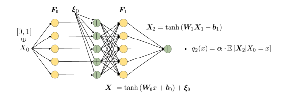
Figure 4: Sketch of the stochastic neural network model used approximate the functions (65) (training over weight paradigm) and (70) (training over noise paradigm). The five-dimensional random vector $\bm{\xi}_{0}$ is assumed to have statistically independent components. We proceed by first training the neural network with no noise on the target function $f(x)$ defined in (65). Subsequently, we perturb the network with the random vector $\bm{\xi}_{0}$, and optimize the PDF of $\bm{\xi}_{0}$ so that the conditional expectation of the neural network output, i.e., (71), approximates a second target function $h(x)$ for the same weights and biases.

In the absence of noise, the output of the network is given by equation (57), hereafter rewritten in full form for $\tanh(\cdot)$ activation functions [50]

$$q_{2}(x)= \bm{\alpha}\cdot\tanh\left[\bm{W}_{1}\tanh\left(\bm{W}_{0}x+\bm{b}_{0}\right)+\bm{b}_{1}\right].$$ (66)

Here, $\bm{W}_{0}$, $\bm{b}_{0}$, $\bm{b}_{1}$ and $\bm{\alpha}$ are five-dimensional column vectors, while $\bm{W}_{1}$ is a $5\times 5$ matrix. Hence, the input-output map (66) has $45$ free parameters $\{\bm{W}_{0},\bm{W}_{1},\bm{b}_{0},\bm{b}_{1},\bm{\alpha}\}$ which are determined by minimizing the discrete 2-norm

$$\left\|q_{2}(x)-f(x)\right\|^{2}_{2}=\sum_{i=1}^{30}\left[q_{2}\left(x{[i]}\right)-f\left(x{[i]}\right)\right]^{2},$$ (67)

where $\left\{x{[1]},\ldots,x{[30]}\right\}$ is an evenly-spaced set of points in $[0,1]$

$$x[j]=\frac{(j-1)}{29}\quad j=1,\ldots,30.$$ (68)

In Figure 5 we show the neural network output (66) we obtained by minimizing the cost (67) relative to the weights $\{\bm{W}_{0},\bm{W}_{1},\bm{b}_{0},\bm{b}_{1},\bm{\alpha}\}$ (training over weights paradigm).

Next, we add noise to our fully trained deterministic neural network. Specifically, we perturb the output of the first layer by an additive random vector $\bm{\xi}_{0}$ with independent components supported in $[-0.4,0.4]$. Since the random vector $\bm{\xi}_{0}$ is assumed to have independent components, we can write its PDF $\rho_{0}$ as

$$\rho_{0}(\bm{\xi})=\rho^{1}_{0}\left(\xi_{1}\right)\cdots\rho^{N}_{0}\left(\xi_{N}\right)$$ (69)

where $\{\rho^{1}_{0},\ldots,\rho_{1}^{N}\}$ are one-dimensional PDFs, each one of which is supported in $[-0.4,0.4]$. In the training-over-noise paradigm, we are interested in finding the PDF of the random vector $\bm{\xi}_{0}$, i.e., the one-dimensional PDFs $\{\rho^{1}_{0},\ldots,\rho_{1}^{N}\}$ appearing in (69), and a new vector of coefficients $\bm{\alpha}$ such that the output of the neural network (with the same weights and biases) averaged over all realizations of the noise $\bm{\xi}_{0}$, approximates a new one-dimensional map $h(x)$, different from (65). For this example, we choose

$$h(x)=4\tanh\left(10x-\frac{7}{2}\right)+3.$$ (70)

In the presence of noise, the neural network output takes the form (see Eq. (61))

$$\widehat{q}_{2}(x)=\int_{\mathscr{R}(\bm{\xi}_{0})}\kappa_{2}(x,\bm{\xi})\rho_{0}^{1}(\xi_{1})\cdots\rho_{0}^{5}(\xi_{5})d\xi_{1}\cdots d\xi_{5},$$ (71)

where $\mathscr{R}(\bm{\xi}_{0})=[-0.4,0.4]^{5}$ is the range of $\bm{\xi}_{0}$, and

$$\kappa_{2}(x,\bm{\xi})= \bm{\alpha}\cdot\tanh\left[\bm{W}_{1}\left(\bm{\xi}+\tanh\left(\bm{W}_{0}x+\bm{b}_{0}\right)\right)+\bm{b}_{1}\right].$$ (72)

We approximate the $5$-dimensional integral in (71) with a Gauss-Legendre-Lobatto (GLL) quadrature formula [22] on a tensor-product grid with $6$ quadrature points per dimension. To this end, let $\{z[1],\ldots,z[6]\}$ be the GLL quadrature points in $[-0.4,0.4]$. The tensor product quadrature approximation of (71) takes the form

$$\widehat{q}_{2}(x)\approx\sum_{j=1}^{H}\theta_{j}\kappa_{2}\left(x,\bm{\xi}[j]\right)\rho_{0}^{1}(z[i_{1}(j)])\cdots\rho_{0}^{5}(z[i_{5}(j)]),$$ (73)

where $H=6^{5}=7776$ is the total number of quadrature points in the domain $[-0.4,0.4]^{5}$, $\theta_{k}$ are tensor product GLL quadrature weights, and

$$\bm{\xi}[j]=(z[i_{1}(j)],\ldots,z[i_{5}(j)])$$ (74)

represents a grid in $[-0.4,0.4]^{5}$ indexed by $\{i_{1}(j),\ldots,i_{5}(j)\}$, where $i_{k}(j)\in\{1,\ldots,6\}$ for each $j$ and each $k$. Such indices are obtained by an appropriate ordering of the nodes in the tensor product grid. We represent each one-dimensional PDFs $\rho_{0}^{k}(z)$ using a polynomial interpolant through the GLL points, i.e.,

$$\rho_{0}^{k}(z)\simeq\sum_{j=1}^{6}\rho_{0}^{k}\left(z[j]\right)l_{j}(z),$$ (75)

where $l_{j}(z)$ are Lagrange characteristic polynomials associated with the one-dimensional GLL grid. Thus, the degrees of freedom of each PDF are represented by the following vector of PDF values at the GLL nodes

$$\bm{\rho}_{0}^{k}=\{\rho_{0}^{k}\left(z[1]\right),\ldots,\rho_{0}^{k}\left(z[6]\right)\},\quad k=1,\ldots,5.$$ (76)

Note that in this setting we are approximating the PDF of $\bm{\xi}_{0}$ using a non-parametric method, i.e., a polynomial interpolant through a tensor product GLL grid. For non-separable PDFs, or for PDFs in higher dimensions, it may be more practical to consider a tensor representation [12, 11], or a parametric inference method, i.e., a method that leverages assumptions on the shape of the probability distribution of $\bm{\xi}_{0}$.

At this point, we have all the elements to solve the minimization problem (64), or an equivalent problem defined by the discrete 2-norm

$$\min_{\{\bm{\rho}_{0}^{1},\ldots,\bm{\rho}_{0}^{5},\bm{\alpha}\}}\sum_{i=1}^{S}\left[h(x[i])-\widehat{q}_{2}(x[i])\right]^{2},$$ (77)

subject to the linear constraints

$$\left\|\rho_{0}^{k}\right\|_{L^{1}([-0.4,0.4])}=1,\qquad\rho_{0}^{k}(z)\geq 0\qquad(k=1,\ldots,5).$$ (78)

Training over weights                                                                 Training over noise

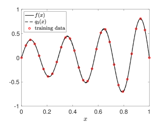
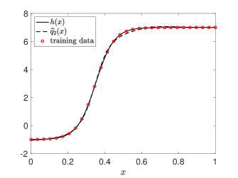
Figure 5: Demonstration of ”training over weights” and “training over noise” paradigms. In the training over weights paradigm we minimize the dissimilarity measure (67) between the output (66) of the two-layer neural network depicted in Figure 4 (with $\bm{\xi}_{0}=\bm{0}$) and the target function (65). The training data is shown with red circles. In the training over noise paradigm we add random noise to the output of the first layer and optimize for $\bm{\alpha}$ and the PDF of the noise as in (64). This can be seen as an instance of transfer learning, in which we keep the neural network weights and biases fixed but update the output weights $\bm{\alpha}$ and the PDF of the random vector $\bm{\xi}_{0}$ to approximate a different function $h(x)$ defined in (70).

In Figure 5 we demonstrate the training-over-weight and the training-over-noise paradigms for the neural network depicted in Figure 4. In the classical training over weight paradigm we minimize the error between the neural network output (66) and the function (65) in the discrete 2-norm (67). The training data is shown with red circles. In the training over noise paradigm we add random noise $\bm{\xi}_{0}$ to the output of the first layer. This yields the input-output map (71). By optimizing for the PDF of the noise $\rho_{0}$ and the coefficients $\bm{\alpha}$ as in (64) we can re-purpose the network previously trained on $f(x)$ to approximate a different function $h(x)$ defined in (70), without changing the neural network weights and biases.

In Figure 6 we plot the one-dimensional PDFs of each component of the random vector $\bm{\xi}_{0}$ we obtained from optimization. Such PDFs depend on the neural network weights and biases, which in this example are kept fixed.

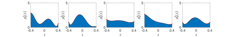
Figure 6: Training over noise paradigm. One-dimensional probability density functions of each component of the random vector $\bm{\xi}_{0}$ obtained by solving the optimization problem (64) for the function $h(x)$ defined in Eq. (70) (see Figure 5). The PDF of $\bm{\xi}_{0}$ is a product of all five PDFs (see Eq. (69)). The degrees of freedom of each PDF, i.e., the vectors defined in equation (76), are visualized as red dots (PDF values at GLL points). Each PDF is a polynomial of degree at most 5.

The PDF of $\bm{\xi}_{0}$ is (by hypothesis) a product of five one-dimensional PDFs. Therefore it is quite straightforward to sample $\bm{\xi}_{0}$ by using, e.g., rejection sampling applied independently to each one-dimensional PDF shown in Figure 6. With the samples of $\bm{\xi}_{0}$ available, we can easily compute samples of the neural network output as

$$\tilde{q}_{2}(x)=\bm{\alpha}\cdot\tanh\left[\bm{W}_{1}\left(\bm{\xi}_{0}+\tanh\left(\bm{W}_{0}x+\bm{b}_{0}\right)\right)+\bm{b}_{1}\right].$$ (79)

Clearly, if we compute an ensemble average over a large number of output samples then we obtain an approximation of $\widehat{q}_{2}(x)$. This is demonstrated in Figure 7.

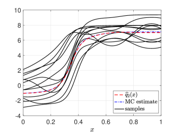
Figure 7: Training over noise paradigm. Samples of the stochastic neural network output (79) corresponding to random samples of $\bm{\xi}_{0}$. We also show that the ensemble average of the network output computed over $10^{5}$ independent samples of (79) converges to $\widehat{q}_{2}(x)$, as expected.

4.2.1 Random shifts

A related but simpler setting for re-purposing a neural network is to introduce a random shift in the input variable rather than perturbing the network layers. In this setting, the output of the network can be written as

$$r_{2}(\bm{x})=\int q_{2}(\bm{x}-\bm{y})\rho\left(\bm{y}\right)d\bm{y},$$ (80)

where $q_{2}$ is defined in (57), and $\rho$ is the PDF of vector $\bm{\eta}$ defining the random shift $\bm{x}\rightarrow\bm{x}-\bm{\eta}$. Clearly, equation (60) is the expectation of the noiseless neural network output $q_{2}(\bm{x})$ under a random shift with PDF $\rho(\bm{y})$. To re-purpose a deterministic neural net using random shifts in the input variable one can proceed by optimization, i.e., solving an optimization problem similar to (64) for a target function $h(\bm{x})$.

Remark: Given a target function $h(\bm{x})$ we can, in principle, compute the analytical solution of the integral equation

$$h(\bm{x})=\int q_{2}(\bm{x}-\bm{y})\rho\left(\bm{y}\right)d\bm{y},\qquad\bm{x},\bm{y}\in\mathbb{R}^{d}$$ (81)

using Fourier transforms. This yields

$$\rho\left(\bm{y}\right)=\int\frac{\mathcal{F}[h(\bm{x})](\bm{\zeta})}{\mathcal{F}[q_{2}(\bm{x})](\bm{\zeta})}e^{2\pi i\bm{\zeta}\cdot\bm{x}}d\bm{\zeta},$$ (82)

where $\mathcal{F}[\cdot]$ denotes the multivariate Fourier transform operator

$$\mathcal{F}[f(\bm{x})](\bm{\zeta})=\int f(\bm{x})e^{-2\pi i\bm{x}\cdot\bm{\zeta}}d\bm{x}.$$ (83)

However, the function $\rho(\bm{y})$ defined in (82) is, in general, not a PDF.

5 The Mori-Zwanzig formulation of deep learning

In section 3 we defined two linear operators, i.e., $\mathcal{N}(n,q)$ and $\mathcal{M}(n,q)$ in equations (13) and (19), mapping the probability density of the state $\bm{X}_{n}$ and the conditional expectation of a phase space function $\bm{u}(\bm{X}_{n})$ forward or backward across different layers of the neural network. In particular, we have shown that

$$p_{n+1}(\bm{x}) =\mathcal{N}(n+1,n)p_{n}(\bm{x}),$$ (84)

$$\mathbb{E}\{\bm{u}(\bm{X}_{L})|\bm{X}_{n}=\bm{x}\} =\mathcal{M}(n,n+1)\mathbb{E}\{\bm{u}(\bm{X}_{L})|\bm{X}_{n+1}=\bm{x}\}.$$ (85)

Equation (84) maps the PDF of the state $\bm{X}_{j}$ forward through the neural network, i.e., from the input to the output as $n$ increases, while (85) maps the conditional expectation backward. We have also shown in section 3.2 that upon definition of

$$\bm{q}_{n}(\bm{x})=\mathbb{E}\{\bm{u}(\bm{X}_{L})|\bm{X}_{L-n}=\bm{x}\}$$ (86)

we can rewrite (85) as a forward propagation problem, i.e.,

$$\bm{q}_{n+1}(\bm{x})=\mathcal{G}(n+1,n)\bm{q}_{n}(\bm{x}),$$ (87)

where $\mathcal{G}(n,q)=\mathcal{M}(L-n,L-q)$ and $\mathcal{M}$ is defined in (19). The function $\bm{q}_{n}(\bm{x})$ is defined on the domain

$$\mathscr{R}(\bm{X}_{L-n})=\{\bm{X}_{L-n}(\omega)\in\mathbb{R}^{N}\,:\,\omega\in\mathcal{S}\},$$ (88)

i.e., on the range of the random variable $\bm{X}_{L-n}(\omega)$ (see Definition (188)). $\mathscr{R}(\bm{X}_{L-n})$ is a deterministic subset of $\mathbb{R}^{N}$.

Eqs. (85) constitute the basis for developing the Mori-Zwanzig (MZ) formulation of deep neural networks. The MZ formulation is a technique originally developed in statistical mechanics [41, 64] to formally integrate out phase variables in nonlinear dynamical systems by means of a projection operator. One of the main features of such formulation is that it allows us to systematically derive exact equations for quantities of interest, e.g., low-dimensional observables, based on the equations of motion of the full system. In the context of deep neural networks such equations of motion are Eqs. (84)-(85), and (87).

To develop the Mori-Zwanzig formulation of deep learning, we introduce a layer-dependent orthogonal projection operator $\mathcal{P}_{n}$ together with the complementary projection $\mathcal{Q}_{n}=\mathcal{I}-\mathcal{P}_{n}$. The nature and properties of $\mathcal{P}_{n}$ will be discussed in detail in section 6. For now, it suffices to assume only that $\mathcal{P}_{n}$ is a self-adjoint bounded linear operator, and that $\mathcal{P}_{n}^{2}=\mathcal{P}_{n}$, i.e., $\mathcal{P}_{n}$ is idempotent. To derive the MZ equation for neural networks, let us consider a general recursion,

$$\bm{g}_{n+1}(\bm{x})=\mathcal{R}(n+1,n)\bm{g}_{n}(\bm{x}),$$ (89)

where $\{\bm{g}_{n},\mathcal{R}(n+1,n)\}$ can be either $\{p_{n},\mathcal{N}(n+1,n)\}$ or $\{\bm{q}_{n},\mathcal{G}(n+1,n)\}$, depending on the context of the application.

5.1 The projection-first and propagation-first approaches

We apply the projection operators $\mathcal{P}_{n}$ and $\mathcal{Q}_{n}$ to (89) to obtain the following coupled system of equations

$$\bm{g}_{n+1}= \mathcal{R}(n+1,n)\mathcal{P}_{n}\bm{g}_{n}+\mathcal{R}(n+1,n)\mathcal{Q}_{n}\bm{g}_{n},$$ (90)

$$\mathcal{Q}_{n+1}\bm{g}_{n+1}= \mathcal{Q}_{n+1}\mathcal{R}(n+1,n)\mathcal{P}_{n}\bm{g}_{n}+\mathcal{Q}_{n+1}\mathcal{R}(n+1,n)\mathcal{Q}_{n}\bm{g}_{n}.$$ (91)

By iterating the difference equation (91), we obtain the following formula for $\mathcal{Q}_{n}\bm{g}_{n}$

$$\mathcal{Q}_{n}\bm{g}_{n}=\Phi_{\mathcal{R}}(n,0)\mathcal{Q}_{0}\bm{g}_{0}+\sum_{m=0}^{n-1}\Phi_{\mathcal{R}}(n,m)\mathcal{P}_{m}\bm{g}_{m},$$ (94)

where $\Phi_{\mathcal{R}}(n,m)$ is the (forward) propagator of the orthogonal dynamics, i.e.,

$$\Phi_{\mathcal{R}}(n,m)=\mathcal{Q}_{n}\mathcal{R}(n,n-1)\cdots\mathcal{Q}_{m+1}\mathcal{R}(m+1,m).$$ (95)

Since $\bm{g}_{n}=\mathcal{R}(n,0)\bm{g}_{0}$, and $\bm{g}_{0}$ is arbitrary, we have that (94) implies the operator identity

$$\mathcal{Q}_{n}\mathcal{R}(n,0)=\Phi_{\mathcal{R}}(n,0)\mathcal{Q}_{0}+\sum_{m=0}^{n-1}\Phi_{\mathcal{R}}(n,m)\mathcal{P}_{m}\mathcal{R}(m,0).$$ (96)

A substitution of (94) into (90) yields the Mori-Zwanzig equation

$$\bm{g}_{n+1}=\underbrace{\mathcal{R}(n+1,n)\mathcal{P}_{n}\bm{g}_{n}}_{\text{streaming term}}+\underbrace{\mathcal{R}(n+1,n)\Phi_{\mathcal{R}}(n,0)\mathcal{Q}_{0}\bm{g}_{0}}_{\text{noise term}}+\underbrace{\mathcal{R}(n+1,n)\sum_{m=0}^{n-1}\Phi_{\mathcal{R}}(n,m)\mathcal{P}_{m}\bm{g}_{m}}_{\text{memory term}}.$$ (97)

We shall call the first term at the right hand side of (97) streaming (or Markovian) term, in agreement with classical literature on MZ equations. The streaming term represents the change in $\mathcal{P}_{n}\bm{g}_{n}$ as we go from one layer to the next. The second term is known as “noise term” in classical statistical mechanics. The reason for this definition is that $\Phi_{\mathcal{R}}(n,0)\mathcal{Q}_{0}\bm{g}_{0}$ represents the effects of the dynamics generated by $\mathcal{Q}_{m}\mathcal{R}(m,m-1)$, which is usually under-resolved in classical particle systems and therefore modeled as random noise. Such noise, however, is very different from the random noise $\{\bm{\xi}_{0},\ldots,\bm{\xi}_{L-1}\}$ we introduced into the neural network model (1). The third term represents the memory of the neural network, and it encodes the interaction between the projected dynamics and its entire history.

Note that if $\bm{g}_{0}$ is in the range of $\mathcal{P}_{0}$, i.e., if $\mathcal{P}_{0}\bm{g}_{0}=\bm{g}_{0}$, then the second term drops out, yielding a simplified MZ equation,

$$\bm{g}_{n+1}=\mathcal{R}(n+1,n)\mathcal{P}_{n}\bm{g}_{n}+\mathcal{R}(n+1,n)\sum_{m=0}^{n-1}\Phi_{\mathcal{R}}(n,m)\mathcal{P}_{m}\bm{g}_{m}.$$ (98)

To integrate (98) forward, i.e., from one layer to the next, we first project $\bm{g}_{m}$ using $\mathcal{P}_{m}$ (for $m=0,\ldots,n$), then apply the evolution operator $\mathcal{R}(n+1,n)$ to $\mathcal{P}_{n}\bm{g}_{n}$, and the memory operator $\Phi_{\mathcal{R}}$ to the entire history of $\bm{g}_{m}$ (memory of the network). It is also possible to construct an MZ equation based on the reversed mechanism, i.e., by projecting $\mathcal{R}(n+1,n)\bm{g}_{n}$ rather than $\bm{g}_{m}$. To this end, re-write (90) as

$$\bm{g}_{n+1}=\mathcal{P}_{n+1}\mathcal{R}(n+1,n)\bm{g}_{n}+\mathcal{Q}_{n+1}\mathcal{R}(n+1,n)\bm{g}_{n},$$ (99)

i.e., the propagation via $\mathcal{R}(n+1,n)$ precedes projection (propagation-first approach). By applying the variation of constant formula (96) to (99) we arrive at a slightly different (though completely equivalent) form of the MZ equation, namely

$$\bm{g}_{n+1}=\mathcal{P}_{n+1}\mathcal{R}(n+1,n)\bm{g}_{m}+\Phi_{\mathcal{R}}(n+1,0)\bm{g}_{0}+\sum_{m=0}^{n-1}\Phi_{\mathcal{R}}(n+1,m+1)\mathcal{P}_{m+1}\mathcal{R}(m+1,m)\bm{g}_{m}.$$ (100)

5.2 Discrete Dyson’s identity

Another form of the MZ equation (97) can be derived based on a discrete version of the Dyson identity. To derive this identity, consider the sequence

$$\bm{y}_{n+1}= \mathcal{Q}_{n+1}\mathcal{R}(n+1,n)\bm{y}_{n}$$ (102)

$$= \mathcal{R}(n+1,n)\bm{y}_{n}-\mathcal{P}_{n+1}\mathcal{R}(n+1,n)\bm{y}_{n}.$$ (103)

By using the discrete variation of constant formula, we can rewrite (103) as

$$\bm{y}_{n}=\mathcal{R}(n,0)\bm{y}_{0}-\sum_{m=0}^{n-1}\mathcal{R}(n,m+1)\mathcal{P}_{m+1}\mathcal{R}(m+1,m)\bm{y}_{m}.$$ (104)

Similarly, solving (102) yields

$$\bm{y}_{n}=\Phi_{\mathcal{R}}(n,0)\bm{y}_{0},$$ (105)

where $\Phi_{\mathcal{R}}$ is defined in (95). By substituting (105) into (104) for both $\bm{y}_{n}$ and $\bm{y}_{m}$, and observing that $\bm{y}_{0}$ is arbitrary, we obtain

$$\mathcal{R}(n,0)=\Phi_{\mathcal{R}}(n,0)+\sum_{m=0}^{n-1}\mathcal{R}(n,m+1)\mathcal{P}_{m+1}\mathcal{R}(m+1,m)\Phi_{\mathcal{R}}(m,0).$$ (106)

The operator identity (106) is the discrete version of the well-known continuous-time Dyson’s identity. A substitution of (106) into $\bm{g}_{n}=\mathcal{R}(n,0)\bm{g}_{0}$ yields the following form of the MZ equation (97)

$$\bm{g}_{n+1}=\mathcal{P}_{n+1}\mathcal{R}(n+1,n)\Phi_{\mathcal{R}}(n,0)\bm{g}_{0}+\Phi_{\mathcal{R}}(n+1,0)\bm{g}_{0}+\sum_{m=0}^{n-1}\mathcal{R}(n+1,m+1)\mathcal{P}_{m+1}\mathcal{R}(m+1,m)\Phi_{\mathcal{R}}(m,0)\bm{g}_{0}.$$ (107)

Here we have arranged the terms in the same way as in (97).

5.3 Mori-Zwanzig equations for probability density functions

We have seen that the PDF of the random vector $\bm{X}_{n}$ can be mapped forward and backward through the neural network via the transfer operator $\mathcal{N}(q,n)$ in (13). Replacing $\mathcal{R}$ with $\mathcal{N}$ in (97) yields the following Mori-Zwanzig equation for the PDF of $\bm{X}_{n}$

$$p_{n+1}=\underbrace{\mathcal{N}(n+1,n)\mathcal{P}_{n}p_{n}}_{\text{streaming term}}+\underbrace{\mathcal{N}(n+1,n)\Phi_{\mathcal{N}}(n,0)\mathcal{Q}_{0}p_{0}}_{\text{noise term}}+\underbrace{\mathcal{N}(n+1,n)\sum_{m=0}^{n-1}\Phi_{\mathcal{N}}(n,m)\mathcal{P}_{m}p_{m}}_{\text{memory term}},$$ (108)

Alternatively, by using the MZ equation (107), we can write

$$p_{n}=\Phi_{\mathcal{N}}(n,0)p_{0}+\sum_{m=0}^{n-1}\mathcal{N}(n,m+1)\mathcal{P}_{m+1}\mathcal{N}(m+1,m)\Phi_{\mathcal{N}}(m,0)p_{0},$$ (109)

where

$$\Phi_{\mathcal{N}}(n,m)=\mathcal{Q}_{n}\mathcal{N}(n,n-1)\cdots\mathcal{Q}_{m+1}\mathcal{N}(m+1,m).$$ (110)

5.4 Mori-Zwanzig equation for conditional expectations

Next, we discuss MZ equations in neural nets propagating conditional expectations

$$\bm{q}_{n}(\bm{x})=\mathbb{E}\{\bm{u}(\bm{X}_{L})|\bm{X}_{L-n}=\bm{x}\}$$ (111)

backward across the network, i.e., from $\bm{q}_{0}(\bm{x})=\bm{u}(\bm{x})$ into $\bm{q}_{L}(\bm{x})=\mathbb{E}\{\bm{u}(\bm{X}_{L})|\bm{X}_{0}=\bm{x}\}$. To simplify the notation, we denote the projection operators in the space of conditional expectations with the same letters as in the space of PDFs, i.e., $\mathcal{P}_{n}$ and $\mathcal{Q}_{n}$. Replacing $\mathcal{R}$ with $\mathcal{G}$ in (97) yields the following MZ equation for the conditional expectations

$$\bm{q}_{n+1}=\underbrace{\mathcal{G}(n+1,n)\mathcal{P}_{n}\bm{q}_{n}}_{\text{streaming term}}+\underbrace{\mathcal{G}(n+1,n)\Phi_{\mathcal{G}}(n,0)\mathcal{Q}_{0}\bm{q}_{0}}_{\text{noise term}}+\underbrace{\mathcal{G}(n+1,n)\sum_{m=0}^{n-1}\Phi_{\mathcal{G}}(n,m)\mathcal{P}_{m}\bm{q}_{m}}_{\text{memory term}},$$ (113)

where

$$\Phi_{\mathcal{G}}(n,m)=\mathcal{Q}_{n}\mathcal{G}(n,n-1)\cdots\mathcal{Q}_{m+1}\mathcal{G}(m+1,m).$$ (114)

Equation (113) can be equivalently written by incorporating the streaming term into the summation of the memory term

$$\bm{q}_{n+1}=\mathcal{G}(n+1,n)\Phi_{\mathcal{G}}(n,0)\mathcal{Q}_{0}\bm{q}_{0}+\mathcal{G}(n+1,n)\sum_{m=0}^{n}\Phi_{\mathcal{G}}(n,m)\mathcal{P}_{m}\bm{q}_{m}.$$ (115)

Alternatively, by using Eq. (107) we obtain

$$\bm{q}_{n}=\Phi_{\mathcal{G}}(n,0)\bm{q}_{0}+\sum_{m=0}^{n-1}\mathcal{G}(n,m+1)\mathcal{P}_{m+1}\mathcal{G}(m+1,m)\Phi_{\mathcal{G}}(m,0)\bm{q}_{0}.$$ (116)

Remark: The Mori-Zwanzig equations (108)-(109) and (113)-(116) allow us to perform dimensional reduction within each layer of the network (number of neurons per layer, via projection), or across different layers (total number of layers, via memory approximation). The MZ formulation is also useful to perform theoretical analysis of deep learning by using tools from operator theory. As we shall see in section 7, the memory of the neural network can be controlled by controlling the noise process $\{\bm{\xi}_{0},\bm{\xi}_{1},\ldots,\bm{\xi}_{L-1}\}$.

6 Mori-Zwanzig projection operator

Suppose that the neural network model (2) is perturbed by independent random variables $\{\bm{\xi}_{n}\}$ with bounded range $\mathscr{R}(\bm{\xi}_{n})$. In this hypothesis, the range of each random vector $\bm{X}_{m}$, i.e. $\mathscr{R}(\bm{X}_{m})$, is bounded. In fact,

$$\mathscr{R}(\bm{X}_{m})\subseteq\Omega_{m}=\{\bm{c}\in\mathbb{R}^{N}:\,\bm{c}=\bm{a}+\bm{b}\quad\bm{a}\in[-1,1]^{N},\quad\bm{b}\in\mathscr{R}(\bm{\xi}_{m-1})\},$$ (117)

and $\Omega_{m}$ is clearly a bounded set if $\mathscr{R}(\bm{\xi}_{m-1})$ is bounded. With specific reference to MZ equations for scalar conditional expectations (i.e., conditional averages of scalar quantities of interest)

$$q_{m}(\bm{x})=\mathbb{E}\left[u(\bm{X}_{L})|\bm{X}_{L-m}=\bm{x}\right],$$ (118)

and recalling that

$$q_{m}(\bm{x})= \mathcal{G}(m,m-1)q_{m-1}$$

$$= \mathcal{M}(L-m,L-m+1)q_{m-1}(\bm{x})$$

$$= \int_{\mathscr{R}(\bm{X}_{L-m+1})}\underbrace{p_{L-m+1|L-m}(\bm{y},\bm{x})}_{\rho_{L-m}(\bm{y}-\bm{F}_{L-m}\left(\bm{x},\bm{w}_{L-m})\right)}q_{m-1}(\bm{y})d\bm{y},$$ (119)

we define the following orthogonal projection operator on $L^{2}(\mathscr{R}(\bm{X}_{L-m}))$

$$\mathcal{P}_{m}:L^{2}(\mathscr{R}(\bm{X}_{L-m})) \mapsto L^{2}(\mathscr{R}(\bm{X}_{L-m}))$$

$$f \mapsto\mathcal{P}_{m}f=\int_{\mathscr{R}(\bm{X}_{L-m})}K_{L-m}(\bm{x},\bm{y})f(\bm{y})d\bm{y}.$$ (120)

Since $\mathcal{P}_{m}$ is, by definition, an orthogonal projection we have that $\mathcal{P}_{m}$ is idempotent ($\mathcal{P}_{m}^{2}=\mathcal{P}_{m}$), bounded, and self-adjoint relative to the inner product in $L^{2}\left(\mathscr{R}(\bm{X}_{L-m})\right)$. These conditions imply that the kernel $K_{L-m}(\bm{x},\bm{y})$ is a symmetric Hilbert-Schmidt kernel that satisfies the reproducing kernel condition

$$\int_{\mathscr{R}(\bm{X}_{L-m})}K_{L-m}(\bm{x},\bm{y})K_{L-m}(\bm{y},\bm{z})d\bm{y}=K_{L-m}(\bm{x},\bm{z}),\qquad\forall\bm{x},\bm{z}\in\mathscr{R}(\bm{X}_{L-m}).$$ (121)

Note that the classical Mori’s projection [61, 60] can be written in the form (120) if we set

$$K_{L-m}(\bm{x},\bm{y})=\sum_{i=0}^{M}\eta^{m}_{i}(\bm{x})\eta^{m}_{i}(\bm{y}),$$ (122)

where $\{\eta^{m}_{0},\ldots,\eta^{m}_{M}\}$ are orthonormal functions in $L^{2}\left(\mathscr{R}(\bm{X}_{L-m})\right)$. Since the range of $\bm{X}_{L-m}$ can vary from layer to layer we have that the set of orthonormal functions $\{\eta^{m}_{j}(\bm{x})\}$ also depends on the layer (hence the label “$m$”). The projection operator $\mathcal{P}_{m}$ is said to be non-negative if for all positive functions $v(\bm{x})\in L_{\mu_{m}}^{2}(\mathscr{R}(\bm{X}_{L-m}))$ ($v>0$) we have that $\mathcal{P}_{m}v\geq 0$ [26]. Clearly, this implies that the kernel $K_{L-m}(\bm{x},\bm{y})$ is non-negative in $\mathscr{R}(\bm{X}_{L-m})\times\mathscr{R}(\bm{X}_{L-m})$ [17]. An example of a kernel defining a non-negative orthogonal projection is

$$K_{L-m}(\bm{x},\bm{y})=\eta^{m}(\bm{x})\eta^{m}(\bm{y}),\qquad\eta^{m}(\bm{x})\geq 0,\qquad\left\|\eta^{m}\right\|_{L_{\mu_{m}}^{2}(\mathscr{R}(\bm{X}_{L-m}))}=1.$$ (123)

More generally, if $K_{L-m}(\bm{x},\bm{y})$ is any square-integrable symmetric conditional probability density function on $\mathscr{R}(\bm{X}_{L-m})\times\mathscr{R}(\bm{X}_{L-m})$, then $\mathcal{P}_{m}$ is a non-negative projection.

7 Analysis of the MZ equation

We now turn to the theoretical analysis of the MZ equation. In particular, we study the MZ equation for conditional expectations discussed in section 5.4, i.e., equation (113). Clearly, the operator $\mathcal{Q}_{m}\mathcal{G}(m,m-1)$ plays a very important role in such an equation via the memory operator $\Phi_{\mathcal{G}}$ defined in (114). Indeed, $\Phi_{\mathcal{G}}$ appears in both the memory term and the noise term, and is defined by operator products involving $\mathcal{Q}_{m}\mathcal{G}(m,m-1)$.

In this section, we aim at determining conditions on $Q_{m}\mathcal{G}(m,m-1)=(\mathcal{I}-\mathcal{P}_{m})\mathcal{G}(m,m-1)$, e.g., noise level and distribution, such that

$$\left\|\mathcal{Q}_{m}\mathcal{G}(m,m-1)\right\|=\sup_{\begin{subarray}{c}v\in L^{2}(\mathscr{R}(\bm{X}_{L-m+1}))\\ v\neq 0\end{subarray}}\frac{\left\|\mathcal{Q}_{m}\mathcal{G}(m,m-1)v\right\|_{L^{2}(\mathscr{R}(\bm{X}_{L-m}))}}{\left\|v\right\|_{L^{2}(\mathscr{R}(\bm{X}_{L-m+1}))}}<1.$$ (124)

In this way, the operator $\mathcal{Q}_{m}\mathcal{G}(m,m-1)$ becomes a contraction, and therefore the MZ memory term in (113) decays with the number of layers, while the noise term decays zero. Indeed, if (124) holds true, then the norm of memory operator $\Phi_{\mathcal{G}}(n,m)$ defined in (114) (similar in (115) and (116) ) decays with the number of “$\mathcal{Q}\mathcal{G}$” operator products taken, i.e., with the number of layers.

7.1 Deterministic neural networks

Before turning to the theoretical analysis of the operator $\mathcal{Q}_{m}\mathcal{G}(m,m-1)$, it is convenient to dwell on the case where the neural network is deterministic (no random perturbations), and has $\tanh()$ activation functions. This case is quite common in practical applications, and also allows for significant simplifications of the MZ framework. First of all, in the absence of noise the output of each neural network layer has the same range, i.e.,

$$\mathscr{R}\left(\bm{X}_{n}\right)=[-1,1]^{N}\qquad n=1,\ldots,L,$$ (125)

where $N$ is the number of neurons, assumed to be constant for each layer. Hence, we can choose a projection operator (120) that does not depend on the particular layer. For simplicity, we consider

$$\mathcal{P}f=\int_{[-1,1]^{N}}K(\bm{x},\bm{y})f(\bm{y})d\bm{y},$$ (126)

where

$$K(\bm{x},\bm{y})=\eta_{0}+\sum_{k=1}^{M}\eta_{k}(\bm{x})\eta_{k}(\bm{y}).$$ (127)

Here $\{\eta_{0},\ldots,\eta_{M}\}$ are orthonormal functions in $L^{2}\left([-1,1]^{N}\right)$, e.g., normalized multivariate Legendre polynomials [57]. We sort $\{\eta_{k}\}$ based on degree lexicographic order. In this way, the first $N+1$ orthonormal functions in (127) are explicitly written as

$$\eta_{0}=2^{-N/2},\qquad\eta_{k}(\bm{x})=2^{-N/2}\sqrt{3}x_{k}\qquad k=1,\ldots,N.$$ (128)

Moreover, if the neural network has linear output we have $q_{0}(\bm{x})=\bm{\alpha}\cdot\bm{x}$ and therefore

$$\mathcal{P}q_{0}=q_{0}\qquad\mathcal{Q}q_{0}=(\mathcal{I}-\mathcal{P})q_{0}=0.$$ (129)

This implies that the noise term in the MZ equation (113) is zero for the projection kernel (127)-(128) and networks with linear output.

To study the MZ memory term we consider a simple example involving a two-layer deterministic neural net with $d$-dimensional input $\bm{x}\in\Omega_{0}\subseteq\mathbb{R}^{d}$ and scalar output $q_{2}(\bm{x})$. The MZ equation (113) with projection operator (126)-(128) can be written as

$$q_{2}(\bm{x})=\mathcal{G}(2,1)\mathcal{P}q_{1}+\underbrace{\mathcal{G}(2,1)\left[q_{1}-\mathcal{P}q_{1}\right]}_{\text{memory term}},\qquad\bm{x}\in\Omega_{0}.$$ (130)

Clearly, if $q_{1}$ is approximately in the range of $\mathcal{P}$ (i.e., if $q_{1}\simeq\mathcal{P}q_{1}$) then the neural network is essentially memoryless (the memory term in (130) drops out). The next question is whether the nonlinear function $q_{1}$ can indeed be approximated accurately by $\mathcal{P}q_{1}$. This is a well-established result in multivariate polynomial approximation theory. In particular, it can be shown that $\mathcal{P}q_{1}$ converges exponentially fast to $q_{1}$as we increase the polynomial degree in the multivariate Legendre expansion (i.e., as we increase $M$ in (127)). Exponential convergence follows immediately from the fact that the function

$$q_{1}(\bm{x}) =\mathcal{G}(1,0)q_{0}$$

$$=\bm{\alpha}\cdot\tanh(\bm{W}_{1}\bm{x}+\bm{b}_{1}),\qquad\bm{x}\in[-1,1]^{N}$$ (131)

admits an analytical extension on a Bernstein poly-ellipse enclosing $[-1,1]^{N}$ (see [57] for details). The projection of the nonlinear function $q_{1}(\bm{x})$ onto the linear space spanned by the $N+1$ orthonormal basis functions (128) (i.e., the space of affine functions defined on $[-1,1]^{N}$) can be written as

$$\mathcal{P}q_{1}=\beta_{0}+\bm{\beta}\cdot\bm{x},$$ (132)

where the coefficients $\{\beta_{0},\ldots,\beta_{N}\}$ are given by

$$\beta_{0}=\frac{1}{2^{N}}\int_{[-1,1]^{N}}q_{1}(\bm{x})d\bm{x},\qquad\beta_{j}=\frac{3}{2^{N}}\int_{[-1,1]^{N}}q_{1}(\bm{x})x_{j}d\bm{x}\qquad j=1,\ldots,N.$$ (133)

Hence, if $q_{1}$ is approximately in the range of $\mathcal{P}$ (i.e., $\mathcal{P}q_{1}\simeq q_{1}$), then we can explicitly write the MZ equation (130) as

$$q_{2}(\bm{x})\simeq\beta_{0}+\bm{\beta}\cdot\tanh(\bm{W}_{0}\bm{x}+\bm{b}_{0}),\qquad\bm{x}\in\Omega_{0}.$$ (134)

Note that this reduces the total number of degrees of freedom of the two-layer neural network from $N(N+d+3)$ to $N(d+2)+1$, under the condition that $q_{1}$ in equation (131) can be accurately approximated by the hyperplane $\mathcal{P}q_{1}$ in equation (132). This depends of course on the weights $\bm{W}_{1}$ and biases $\bm{b}_{1}$ in (131). In particular, if the entries of the weight matrix $\bm{W}_{1}$ are sufficiently small then by using Taylor series it is immediate to prove that $\mathcal{P}q_{1}\simeq q_{1}$.

An example: In Figure 8 we compare the MZ streaming and memory terms for the two-layer deterministic neural network we studied in section 4 and the target function (65). Here we consider $N=20$ neurons, and approximate the integrals in (133) using Monte Carlo quadrature. Clearly, it is possible to constrain the norm of the weight matrix $\bm{W}_{1}$ during training so that the nonlinear function $q_{1}$ in (131) is approximated well by the affine function $\mathcal{P}q_{1}$ in (132). This essentially allows us to control the approximation error $\left\|q_{1}-\mathcal{P}q_{1}\right\|_{L^{2}([-1,1]^{N})}$ and therefore the the amplitude of the MZ memory term in (130). For this particular example, we set $\left\|\bm{W}_{1}\right\|_{\infty}\leq 0.1$, which yields the following contraction factor

$$\frac{\left\|\mathcal{Q}\mathcal{G}(2,1)q_{0}\right\|_{L^{2}([-1,1]^{N})}}{\left\|q_{0}\right\|_{L^{2}([-1,1]^{N})}}=\frac{\left\|q_{1}-\mathcal{P}q_{1}\right\|_{L^{2}([-1,1]^{N})}}{\left\|q_{0}\right\|_{L^{2}([-1,1]^{N})}}=7.5\times 10^{-4}.$$ (135)

Note that (135) is not the operator norm of $\mathcal{Q}\mathcal{G}(2,1)$ we defined in (124). In fact, the operator norm requires computing the supremum of $\|\mathcal{Q}\mathcal{G}(2,1)v\|_{L^{2}([-1,1])}/\|v\|_{L^{2}([-1,1])}$ over all nonzero functions $v\in L^{2}([-1,1]^{N})$, not just the linear function $v=q_{0}$ If training-over-weights of deterministic nets is done in a fully unconstrained optimization setting then there is no guarantee that the MZ memory term is small.

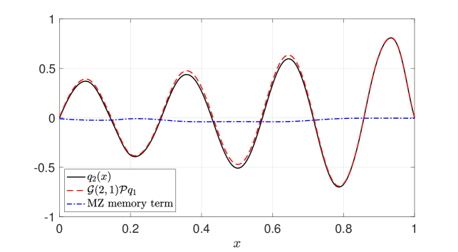
Figure 8: Comparison between the MZ streaming and memory terms for the two-layer deterministic neural network we studied in section 4 and the target function (65). Here we consider $N=20$ neurons, and approximate the high-dimensional integrals in (133) by using Monte Carlo quadrature. The neural network is trained by constraining the entries of the weight matrix $\bm{W}_{1}$ as $\left\|\bm{W}_{1}\right\|_{\infty}\leq 0.1$. This allows us to control the approximation error $\left\|q_{1}-\mathcal{P}q_{1}\right\|_{L^{2}([-1,1]^{N})}$ when projecting the nonlinear function (131) onto the space of affine functions (132) which, in turn, controls the magnitude of the MZ memory term.

The discussion about the approximation of the MZ memory term can be extended to deterministic neural networks with an increasing number of layers. For example, the output of a three-layer deterministic neural network can be written as

$$q_{3}(\bm{x})= \mathcal{G}(3,2)\mathcal{P}q_{2}+\mathcal{G}(3,2)\mathcal{Q}\mathcal{G}(2,1)\mathcal{P}q_{1}+\mathcal{G}(3,2)\mathcal{Q}\mathcal{G}(2,1)\mathcal{Q}\mathcal{G}(1,0)\mathcal{P}q_{0}$$

$$= \mathcal{G}(3,2)\mathcal{P}q_{2}+\underbrace{\mathcal{G}(3,2)\left[\mathcal{I}-\mathcal{P}\right]\mathcal{G}(2,1)\mathcal{P}q_{1}+\mathcal{G}(3,2)\left[\mathcal{I}-\mathcal{P}\right]\mathcal{G}(2,1)\left[q_{1}-\mathcal{P}q_{1}\right]}_{\text{memory term}}.$$ (136)

Note that if $\mathcal{P}q_{1}$ is a linear function of the form (132), then the term $\mathcal{G}(3,2)\left[\mathcal{I}-\mathcal{P}\right]\mathcal{G}(2,1)\mathcal{P}q_{1}$ has exactly the same functional form as the MZ memory term $\mathcal{G}(2,1)\left[\mathcal{I}-\mathcal{P}\right]\mathcal{G}(1,0)\mathcal{P}q_{0}=\mathcal{G}(2,1)[q_{1}-\mathcal{P}q_{1}]$. Hence, everything we said about the accuracy of a linear approximation of $\bm{\alpha}\cdot\tanh(\bm{W}_{1}\bm{x}+\bm{b}_{1})$ can be directly applied now to $\mathcal{G}(2,1)\mathcal{P}q_{1}=\bm{\beta}\cdot\tanh(\bm{W}_{2}\bm{x}+\bm{b}_{2})$.

On the other hand, if $q_{1}$ can be approximated with accuracy by the linear function $\mathcal{P}q_{1}$, then the term $\mathcal{G}(2,1)[q_{1}-\mathcal{P}q_{1}]$ is likely to be small. This implies that the last term in (136) is likely to be small as well (bounded operator $\mathcal{G}(3,2)$ applied to the difference between two small functions). In other words, if the weights and biases of the network are such that $q_{1}(\bm{x})=\bm{\alpha}\cdot\tanh(\bm{W}_{n}\bm{x}+b_{n})$ can be approximated with accuracy by the linear function (132) then the MZ memory term of the three-layer network is small.

More generally, by using error estimates for multivariate polynomial approximation of analytic functions [57], it is possible to derive an upper bound for the operator norm of $\mathcal{Q}\mathcal{G}(m,m-1)$ in (124). Such a bound is rather involved, but in principle it allows us to determine conditions on the weights and biases of the neural network such that $\left\|\mathcal{Q}\mathcal{G}(m,m-1)\right\|\leq\kappa$, where $\kappa$ is a given constant smaller than one. This allows us to simplify the memory term in (113) by neglecting terms involving a large number of “$\mathcal{Q}_{m}\mathcal{G}(m,m-1)$” operator products in (114). Hereafter, we determine general conditions for the operator $\mathcal{Q}_{m}\mathcal{G}(m,m-1)$ to be a contraction in the presence of random perturbations.

7.2 Stochastic neural networks

Consider the stochastic neural network model (2) with $L$ layers, $N$ neurons per layer, and transfer functions $\bm{F}_{n}$ with range in $[-1,1]^{N}$ for all $n$. In this section we determine general conditions for the operator $\mathcal{Q}_{m}\mathcal{G}(m,m-1)$ to be a contraction (i.e., to satisfy the inequality (124)) independently of the neural network weights. To this end, we first write the operator $\mathcal{Q}_{m}\mathcal{G}(m,m-1)$ as

$$(\mathcal{Q}_{m}\mathcal{G}(m,m-1)v)(\bm{x}) =\mathcal{Q}_{m}\int_{\mathscr{R}(\bm{X}_{L-m+1})}\underbrace{\rho_{L-m}\left(\bm{y}-\bm{F}_{L-m}(\bm{x},\bm{w}_{L-m})\right)}_{p_{L-m+1|L-m}(\bm{y}|\bm{x})}v(\bm{y})d\bm{y}$$

$$=\int_{\mathscr{R}(\bm{X}_{L-m+1})}\gamma_{L-m}(\bm{y},\bm{x})v(\bm{y})d\bm{y},$$ (137)

where

$$\gamma_{L-m}(\bm{y},\bm{x})=\rho_{L-m}(\bm{y}-\bm{F}_{L-m}(\bm{x},\bm{w}_{L-m}))-\int_{\mathscr{R}(\bm{X}_{L-m})}K_{L-m}(\bm{x},\bm{z})\rho_{L-m}(\bm{y}-\bm{F}_{L-m}(\bm{z},\bm{w}_{L-m}))d\bm{z}.$$ (138)

The conditional density $p_{L-m+1|L-m}(\bm{y}|\bm{x})=\rho_{L-m}(\bm{y}-\bm{F}_{L-m}(\bm{x},\bm{w}_{L-m}))$ is defined on the set

$$\mathscr{B}_{L-m}=\{(\bm{x},\bm{y})\in\mathscr{R}(\bm{X}_{L-m})\times\mathscr{R}(\bm{X}_{L-m+1}):\,(\bm{y}-\bm{F}_{L-m}(\bm{x},\bm{w}_{L-m}))\in\mathscr{R}(\bm{\xi}_{L-m})\}.$$ (139)

As before, we assume that $K_{L-m}$ is an element of $L^{2}(\mathscr{R}(\bm{X}_{L-m})\times\mathscr{R}(\bm{X}_{L-m}))$ and expand it as

$$K_{L-m}(\bm{x},\bm{y})=c_{m}+\sum_{k=1}^{M}\eta^{m}_{i}(\bm{x})\eta^{m}_{i}(\bm{y}),$$ (140)

where $c_{m}$ is a real number and $\eta^{m}_{i}$ are zero-mean orthonormal basis functions in $L^{2}(\mathscr{R}(\bm{X}_{L-m})$, i.e.,

$$\int_{\mathscr{R}(\bm{X}_{L-m})}\eta^{m}_{i}(\bm{x})d\bm{x}=0,\qquad\int_{\mathscr{R}(\bm{X}_{L-m})}\eta^{m}_{i}(\bm{x})\eta^{m}_{j}(\bm{x})d\bm{x}=\delta_{ij}.$$ (141)

Lemma 1.

The kernel (140) satisfies the idempotency requirement (121) if and only if

$$c_{m}=0\qquad\text{or}\qquad c_{m}=\frac{1}{\lambda(\mathscr{R}(\bm{X}_{L-m}))},$$ (142)

where $\lambda(\mathscr{R}(\bm{X}_{L-m}))$ is the Lebesgue measure of the set $\mathscr{R}(\bm{X}_{L-m})$.

Proof.

By substituting (140) into (121) and taking into account (141) we obtain

$$c_{m}^{2}\lambda(\mathscr{R}(\bm{X}_{L-m}))=c_{m},$$ (143)

from which we obtain $c_{m}=0$ or $c_{m}=1/\lambda(\mathscr{R}(\bm{X}_{L-m}))$.

∎

Clearly, if $\mathcal{G}(m,m-1)$ is itself a contraction and $\mathcal{Q}_{m}$ is an orthogonal projection, then the operator product $\mathcal{Q}_{m}\mathcal{G}(m,m-1)$ is a contraction. In the following Proposition, we compute a simple bound for the operator norm of $\mathcal{Q}_{m}\mathcal{G}(m,m-1)$.

Proposition 2.

Let $\mathcal{Q}_{m}$ be an orthogonal projection in $L^{2}(\bm{X}_{L-m})$. Suppose that the PDF of $\bm{\xi}_{L-m}$, i.e. $\rho_{L-m}$, is in $L^{2}(\mathscr{R}(\bm{\xi}_{L-m}))$. Then

$$\left\|\mathcal{Q}_{m}\mathcal{G}(m,m-1)\right\|^{2}\leq\lambda(\Omega_{L-m})\left\|\rho_{L-m}\right\|^{2}_{L^{2}(\mathscr{R}(\bm{\xi}_{L-m}))},$$ (144)

where $\lambda(\Omega_{L-m})$ is the Lebesgue measure of the set $\Omega_{L-m}$ defined in (117) and

$$\left\|\rho_{L-m}\right\|_{L^{2}(\mathscr{R}(\bm{\xi}_{L-m}))}^{2}=\int_{\mathscr{R}(\bm{\xi}_{L-m})}\rho_{L-m}(\bm{x})^{2}d\bm{x}.$$ (145)

In particular, if $\mathcal{G}(m,m-1)$ is a contraction then $\mathcal{Q}_{m}\mathcal{G}(m,m-1)$ is a contraction.

Proof.

The last statement in the Proposition is trivial. In fact, if $\mathcal{Q}_{m}$ is an orthogonal projection then its operator norm is less or equal to one. Hence,

$$\left\|Q_{m}\mathcal{G}(m,m-1)\right\|^{2}\leq\underbrace{\left\|Q_{m}\right\|^{2}}_{\leq 1}\left\|\mathcal{G}(m,m-1)\right\|^{2}.$$ (146)

Therefore if $\mathcal{G}(m,m-1)$ is a contraction and $\mathcal{Q}_{m}$ is an orthogonal projection then $\mathcal{Q}_{m}\mathcal{G}(m,m-1)$ is a contraction. We have shown in A that if $\rho_{L-m}\in L^{2}(\mathscr{R}(\bm{\xi}_{L-m}))$ then $\mathcal{G}(m,m-1)$ is a bounded linear operator from $L^{2}(\mathscr{R}(\bm{X}_{L-m+1})$ to $L^{2}(\mathscr{R}(\bm{X}_{L-m})$. Moreover, the operator norm of $\mathcal{G}(m,m-1)$ can be bounded as (see Eq. (212))

$$\left\|\mathcal{G}(m,m-1)\right\|^{2}\leq\lambda(\Omega_{L-m})\left\|\rho_{L-m}\right\|^{2}_{L^{2}(\mathscr{R}(\bm{\xi}_{L-m}))}.$$ (147)

Hence,

$$\left\|\mathcal{Q}_{m}\mathcal{G}(m,m-1)\right\|^{2}\leq\underbrace{\left\|\mathcal{Q}_{m}\right\|^{2}}_{\leq 1}\lambda(\Omega_{L-m})\left\|\rho_{L-m}\right\|^{2}_{L^{2}(\mathscr{R}(\bm{\xi}_{L-m}))},$$ (148)

which completes the proof of (144).

∎

The upper bound in (144) can be slightly improved using the definition of the projection kernel $K_{L-m}$. This is stated in the following Theorem.

Theorem 3.

Let $K_{L-m}$ be the projection kernel (140) with $c_{m}=1/\lambda(\mathscr{R}(\bm{X}_{L-m}))$. Then the operator norm of $\mathcal{Q}_{m}\mathcal{G}(m,m-1)$ can be bounded as

$$\left\|\mathcal{Q}_{m}\mathcal{G}(m,m-1)\right\|^{2}\leq\lambda(\Omega_{L-m})\left(\left\|\rho_{L-m}\right\|_{L^{2}(\mathscr{R}(\bm{\xi}_{L-m}))}^{2}-\frac{1}{\lambda(\Omega_{L-m+1})}\right).$$ (149)

The upper bound in (149) is independent of the neural network weights.

Proof.

The function $\gamma_{L-m}(\bm{y},\bm{x})$ defined in (138) is a Hilbert-Schmidt kernel. Therefore,

$$\left\|\mathcal{Q}_{m}\mathcal{G}(m,m-1)\right\|^{2}\leq\left\|\gamma_{L-m}\right\|^{2}_{L^{2}(\mathscr{R}(\bm{X}_{L-m+1})\times\mathscr{R}(\bm{X}_{L-m}))}.$$ (150)

The $L^{2}$ norm of $\gamma_{L-m}$ can be written as (see (138))

$$\int_{\mathscr{R}(\bm{X}_{L-m+1})}\int_{\mathscr{R}(\bm{X}_{L-m})}\gamma_{L-m}(\bm{y},\bm{x})^{2}d\bm{y}d\bm{x}=$$

$$\int_{\mathscr{R}(\bm{X}_{L-m+1})}\int_{\mathscr{R}(\bm{X}_{L-m})}\rho_{L-m}(\bm{y}-\bm{F}_{L-m}(\bm{x},\bm{w}_{L-m}))^{2}d\bm{y}d\bm{x}+$$

$$\int_{\mathscr{R}(\bm{X}_{L-m+1})}\int_{\mathscr{R}(\bm{X}_{L-m})}\left(\int_{\mathscr{R}(\bm{X}_{L-m})}K_{L-m}(\bm{x},\bm{z})\rho_{L-m}(\bm{y}-\bm{F}_{L-m}(\bm{z},\bm{w}_{L-m}))d\bm{z}\right)^{2}d\bm{y}d\bm{x}-$$

$$2\int_{\mathscr{R}(\bm{X}_{L-m+1})}\int_{\mathscr{R}(\bm{X}_{L-m})}\rho_{L-m}(\bm{y}-\bm{F}_{L-m}(\bm{x},\bm{w}_{L-m}))\times$$

$$\left(\int_{\mathscr{R}(\bm{X}_{L-m})}K_{L-m}(\bm{x},\bm{z})\rho_{L-m}(\bm{y}-\bm{F}_{L-m}(\bm{z},\bm{w}_{L-m}))d\bm{z}\right)d\bm{y}d\bm{x}.$$ (151)

By using (147), we can write the first term at the right hand side of (151) as

$$\int_{\mathscr{R}(\bm{X}_{L-m+1})}\int_{\mathscr{R}(\bm{X}_{L-m})}\rho_{L-m}(\bm{y}-\bm{F}_{L-m}(\bm{x},\bm{w}_{L-m}))^{2}d\bm{y}d\bm{x}= \left\|\mathcal{G}(m,m-1)\right\|^{2}$$

$$\leq \lambda(\Omega_{L-m})\left\|\rho_{L-m}\right\|_{L^{2}(\mathscr{R}(\bm{\xi}_{L-m}))}^{2}.$$ (152)

A substitution of the series expansion (140) into the second term at the right hand side of (151) yields

$$\int_{\mathscr{R}(\bm{X}_{L-m+1})}\int_{\mathscr{R}(\bm{X}_{L-m})}\left(\int_{\mathscr{R}(\bm{X}_{L-m})}K_{L-m}(\bm{x},\bm{z})\rho_{L-m}(\bm{y}-\bm{F}_{L-m}(\bm{z},\bm{w}_{L-m}))d\bm{z}\right)^{2}d\bm{y}d\bm{x}=$$

$$\frac{1}{\lambda(\mathscr{R}(\bm{X}_{L-m}))}\int_{\mathscr{R}(\bm{X}_{L-m+1})}\left(\int_{\mathscr{R}(\bm{X}_{L-m})}\rho_{L-m}(\bm{y}-\bm{F}_{L-m}(\bm{x},\bm{w}_{L-m}))d\bm{z}\right)^{2}d\bm{y}+$$

$$\sum_{k=1}^{M}\int_{\mathscr{R}(\bm{X}_{L-m+1})}\left(\int_{\mathscr{R}(\bm{X}_{L-m})}\rho_{L-m}(\bm{y}-\bm{F}_{L-m}(\bm{z},\bm{w}_{L-m}))\eta^{m}_{k}(\bm{z})d\bm{z}\right)^{2}d\bm{y}.$$ (153)

Here, we used the fact that the basis functions $\eta^{m}_{k}(\bm{x})$ are zero-mean and orthonormal in $\mathscr{R}(\bm{X}_{L-m})$ (see Eq. (141)). Similarly, by substituting the expansion (140) in the third term at the right hand side of (151) we obtain

$$2\int_{\mathscr{R}(\bm{X}_{L-m+1})}\int_{\mathscr{R}(\bm{X}_{L-m})}\rho_{L-m}(\bm{y}-\bm{F}_{L-m}(\bm{x},\bm{w}_{L-m}))\times$$

$$\left(\int_{\mathscr{R}(\bm{X}_{L-m})}K_{L-m}(\bm{x},\bm{z})\rho_{L-m}(\bm{y}-\bm{F}_{L-m}(\bm{z},\bm{w}_{L-m}))d\bm{z}\right)d\bm{y}d\bm{x}$$

$$=\frac{2}{\lambda(\mathscr{R}(\bm{X}_{L-m}))}\int_{\mathscr{R}(\bm{X}_{L-m+1})}\left(\int_{\mathscr{R}(\bm{X}_{L-m})}\rho_{L-m}(\bm{y}-\bm{F}_{L-m}(\bm{z},\bm{w}_{L-m}))d\bm{z}\right)^{2}d\bm{y}$$

$$+2\sum_{k=1}^{M}\int_{\mathscr{R}(\bm{X}_{L-m+1})}\left(\int_{\mathscr{R}(\bm{X}_{L-m})}\rho_{L-m}(\bm{y}-\bm{F}_{L-m}(\bm{z},\bm{w}_{L-m}))\eta^{m}_{k}(\bm{z})d\bm{z}\right)^{2}d\bm{y}.$$ (154)

Combining (151)-(154) yields

$$\int_{\mathscr{R}(\bm{X}_{L-m+1})}\int_{\mathscr{R}(\bm{X}_{L-m})}\gamma_{L-m}(\bm{y},\bm{x})^{2}d\bm{y}d\bm{x}\leq\lambda(\Omega_{L-m})\left\|\rho_{L-m}\right\|_{L^{2}(\mathscr{R}(\bm{\xi}_{L-m})}^{2}-$$

$$\frac{1}{\lambda(\mathscr{R}(\bm{X}_{L-m}))}\int_{\mathscr{R}(\bm{X}_{L-m+1})}\left(\int_{\mathscr{R}(\bm{X}_{L-m})}\rho_{L-m}(\bm{y}-\bm{F}_{L-m}(\bm{z},\bm{w}_{L-m}))d\bm{z}\right)^{2}d\bm{y}-$$

$$\sum_{k=1}^{M}\int_{\mathscr{R}(\bm{X}_{L-m+1})}\left(\int_{\mathscr{R}(\bm{X}_{L-m})}\rho_{L-m}(\bm{y}-\bm{F}_{L-m}(\bm{z},\bm{w}_{L-m}))\eta^{m}_{k}(\bm{z})d\bm{z}\right)^{2}d\bm{y}.$$ (155)

At this point we use the Cauchy-Schwarz inequality and well-known properties of conditional PDFs to bound the integral in the second term and the integrals in the last summation, respectively, as

$$\frac{\lambda(\mathscr{R}(\bm{X}_{L-m}))^{2}}{\lambda(\mathscr{R}(\bm{X}_{L-m+1}))}\leq\int_{\mathscr{R}(\bm{X}_{L-m+1})}\left(\int_{\mathscr{R}(\bm{X}_{L-m})}\rho_{L-m}(\bm{y}-\bm{F}_{L-m}(\bm{z},\bm{w}_{L-m}))d\bm{z}\right)^{2}d\bm{y},$$ (158)

and

$$\sum_{k=1}^{M}\int_{\mathscr{R}(\bm{X}_{L-m+1})}\left(\int_{\mathscr{R}(\bm{X}_{L-m})}\rho_{L-m}(\bm{y}-\bm{F}_{L-m}(\bm{z},\bm{w}_{L-m}))\eta^{m}_{k}(\bm{z})d\bm{z}\right)^{2}d\bm{y}\geq 0.$$ (159)

By combining (155)-(159) we finally obtain

$$\left\|\mathcal{Q}_{m}\mathcal{G}(m,m-1)\right\|^{2}\leq \left\|\gamma_{L-m}\right\|^{2}_{L^{2}(\mathscr{R}(\bm{X}_{L-m+1})\times\mathscr{R}(\bm{X}_{L-m}))}$$

$$\leq \lambda(\Omega_{L-m})\left(\left\|\rho_{L-m}\right\|_{L^{2}(\mathscr{R}(\bm{\xi}_{L-m}))}^{2}-\frac{1}{\lambda(\Omega_{L-m+1})}\right),$$ (160)

which proves the Theorem.

∎

Remark: The last two terms in (155) represent the $L^{2}$ norm of the projection of $\rho_{L-m}$ onto the orthonormal basis $\{\lambda(\mathscr{R}(\bm{X}_{L-m}))^{-1/2},\eta^{m}_{1},\ldots,\eta^{m}_{M}\}$. If we assume that $\rho_{L-m}(\bm{y}-\bm{F}_{L-m}(\bm{x},\bm{w}_{L-m})$ is in $L^{2}(\mathscr{R}(\bm{X}_{L-m+1})\times\mathscr{R}(\bm{X}_{L-m}))$, then by using Parseval’s identity we can write (151) as

$$\int_{\mathscr{R}(\bm{X}_{L-m+1})}\int_{\mathscr{R}(\bm{X}_{L-m})}\gamma_{L-m}(\bm{y},\bm{x})^{2}d\bm{y}d\bm{x}=$$

$$\sum_{k=M+1}^{\infty}\int_{\mathscr{R}(\bm{X}_{L-m+1})}\left(\int_{\mathscr{R}(\bm{X}_{L-m})}\rho_{L-m}(\bm{y}-\bm{F}(\bm{z},\bm{w}_{L-m}))\eta^{m}_{k}(\bm{z})d\bm{z}\right)^{2}d\bm{y},$$ (161)

where $\{\eta_{M+1},\eta_{M+2}\ldots\}$ is an orthonormal basis for the orthogonal complement (in $L^{2}(\mathscr{R}(\bm{X}_{L-m}))$) of the space spanned by the basis $\{\lambda(\mathscr{R}(\bm{X}_{L-m}))^{-1/2},\eta^{m}_{1},\ldots,\eta^{m}_{M}\}$. This allows us to bound (159) from below (with a nonzero bound). Such lower bound depends on the basis functions $\eta^{m}_{k}$, on the weights $\bm{w}_{L-m}$ as well as on the choice of the transfer function $\bm{F}_{L-m}$. This implies that the bound (149) can be improved, if we provide information on $\eta^{m}_{k}$ and the activation function $\bm{F}$. Note also that the bound (149) is formulated in terms of the Lebesgue measure of $\Omega_{L-m}$, i.e., $\lambda(\Omega_{L-m})$. The reason is that $\lambda(\Omega_{L-m})$ depends only on the range of the noise (see definition (117)), while $\lambda\left(\mathscr{R}(\bm{X}_{L-m})\right)$ depends on the range of the noise, on the weights of the layer $L-m$, and on the range of $\bm{X}_{L-m+1}$.

Lemma 4.

Consider the projection kernel (140) with $c_{m}=1/\lambda(\mathscr{R}(\bm{X}_{L-m}))$ and let $\kappa\geq 0$. If

$$\left\|\rho_{L-m}\right\|_{L^{2}(\mathscr{R}(\bm{\xi}_{L-m}))}^{2}\leq\frac{\kappa}{\lambda(\Omega_{L-m})}+\frac{1}{\lambda(\Omega_{L-m+1})},$$ (162)

then

$$\left\|\mathcal{Q}_{m}\mathcal{G}(m,m-1)\right\|^{2}\leq\kappa.$$ (163)

In particular, if $0\leq\kappa<1$ then $\mathcal{Q}_{m}\mathcal{G}(m,m-1)$ is a contraction.

Proof.

The proof follows immediately from equation (149).

∎

The upper bound in (162) is a slight improvement of the bound we obtained in A, Lemma 19.

7.3 Contractions induced by uniform random noise

Consider the neural network model (2) and suppose that each $\bm{\xi}_{n}$ is a random vector with i.i.d. uniform components supported in $[-b_{n},b_{n}]$ ($b_{n}>0$). In this assumption, the $L^{2}(\mathscr{R}(\bm{\xi}_{L-m}))$ norm of $\rho_{L-m}$ appearing in Theorem 3 and Lemma 4 can be computed analytically as

$$\left\|\rho_{L-m}\right\|_{L^{2}(\mathscr{R}(\bm{\xi}_{L-m}))}^{2}=\frac{1}{\lambda(\mathscr{R}(\bm{\xi}_{L-m}))}=\frac{1}{(2b_{L-m})^{N}},$$ (164)

where $N$ is the number of neurons in each layer. For uniform random variables with independent components it straightforward to show that the Lebesgue measure of the set $\Omega_{L-m}$ defined in (117) and appearing in Lemma 4 is

$$\lambda(\Omega_{L-m})=2^{N}(1+b_{L-m-1})^{N},$$ (165)

i.e.,

$$\lambda(\Omega_{1})=2^{N}(1+b_{0})^{N},\qquad\lambda(\Omega_{2})=2^{N}(1+b_{1})^{N},\qquad\text{etc.}$$ (166)

A substitution of (164) and (165) into the inequality (162) yields

$$\left(\frac{1+b_{L-m-1}}{b_{L-m}}\right)^{N}\leq\kappa+\left(\frac{1+b_{L-m-1}}{1+b_{L-m}}\right)^{N}.$$ (167)

Upon definition of $n=L-m$ this can be written as

$$\frac{b_{n}(b_{n}+1)}{\left[(b_{n}+1)^{N}-b_{n}^{N}\right]^{1/N}}\geq\frac{b_{n-1}+1}{\kappa^{1/N}},\qquad n=1,\ldots,L-1.$$ (168)

A lower bound for the coefficient $b_{0}$ can be set using Proposition 20 in A, i.e.,

$$b_{0}\geq\frac{1}{2}\left(\frac{\lambda(\Omega_{0})}{\kappa}\right)^{1/N}.$$ (169)

With a lower bound for $b_{0}$ available, we can compute a lower bound for each $b_{n}$ ($n=1,2,\ldots$) by solving the recursion (168) with an equality sign.

  $\kappa=0.2$                                                     $\kappa=0.2$

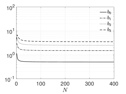
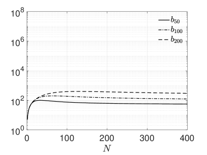
    $\kappa=10^{-4}$                                                    $\kappa=10^{-4}$

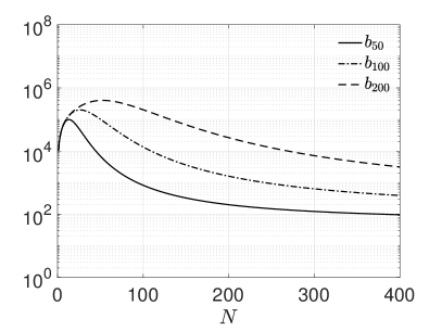
Figure 9: Lower bound on the noise amplitude (168) versus the number of neurons ($N$) for $\lambda(\Omega_{0})=1$ (Lebesgue measure of domain $\Omega_{0}$ defining the neural network input), and different user-defined contraction factors $\kappa$. With these values of $b_{n}$ the operator $\mathcal{Q}_{L-n}\mathcal{G}(L-n,L-n-1)$ is a contraction satisfying $\left\|\mathcal{Q}_{L-n}\mathcal{G}(L-n,L-n-1)\right\|^{2}\leq\kappa$ regardless of the neural network weights and biases.

This is done in Figure 9 for different user-defined contraction factors $\kappa$. It is seen that for a fixed number of neurons $N$, the noise level (i.e., a lower bound for $b_{n}$) that yields operator contractions in the sense of

$$\left\|\mathcal{Q}_{L-n}\mathcal{G}(L-n,L-n-1)\right\|^{2}\leq\kappa,\qquad\kappa<1,\qquad n=1,2\ldots L-1,$$ (171)

increases as we move from the input to the output, i.e.,

$$b_{0}<b_{1}<b_{2}<\cdots<b_{L}.$$ (172)

For instance, for a neural network with layers and $N=100$ neurons per layer the noise amplitude that induces a contraction factor $\kappa=10^{-4}$ independently of the neural network weights is $b_{0}\simeq 0.55$. This means that if each component of the random vector $\bm{\xi}_{0}$ is a uniform random variable with range $[-0.55,0.55]$ then the operator norm of $\mathcal{Q}_{2}\mathcal{G}(2,1)$ is bounded by $10^{-4}$. Moreover, we notice that as we increase the number of neurons $N$, the smallest noise amplitude that satisfies the operator contraction condition

$$\left\|\mathcal{Q}_{L-n}\mathcal{G}(L-n,L-n-1)\right\|^{2}\leq\kappa\qquad\kappa<1,$$ (173)

converges to a constant value that depends on the layer $n$ but not on the contraction factor $\kappa$. Such asymptotic value can be computed analytically.

Lemma 5.

Consider the neural network model (2) and suppose that each perturbation vector $\bm{\xi}_{n}$ has i.i.d. components distributed uniformly in $[-b_{n},b_{n}]$. The smallest noise amplitude $b_{n}$ that satisfies the operator contraction condition (173) satisfies the asymptotic result

$$\lim_{N\rightarrow\infty}b_{n}=\frac{1}{2}+n\qquad n=0,\ldots,L-1$$ (174)

independently of the contraction factor $\kappa$ and $\Omega_{0}$ (domain of the neural network input).

Proof.

The proof follows immediately by substituting the identity

$$\lim_{N\rightarrow\infty}\left[(b_{n}+1)^{N}-b_{n}^{N}\right]^{1/N}=b_{n}+1$$ (175)

into (168). ∎

7.4 Fading property of the neural network memory operator

We now discuss the implications of the contraction property of $\mathcal{Q}_{m}\mathcal{G}(m,m-1)$ on the MZ equation. It is straightforward to show that if Proposition 2 or Lemma 4 holds true then the MZ memory and noise terms in (113) decay with the number of layers. This property is summarized in the following Theorem.

Theorem 6.

If the conditions of Lemma 4 are satisfied, then the MZ memory operator in Equation (114) decays with the number of layers in the neural network, i.e.,

$$\left\|\Phi_{\mathcal{G}}(n,m+1)\right\|^{2}\geq\frac{1}{\kappa}\left\|\Phi_{\mathcal{G}}(n,m)\right\|^{2}\qquad\forall n\geq m+1,\qquad 0<\kappa<1.$$ (176)

Moreover,

$$\left\|\Phi_{\mathcal{G}}(n,0)\right\|^{2}\leq\kappa^{n},$$ (177)

i.e., the memory operator $\Phi_{\mathcal{G}}(n,0)$ decays exponentially fast with the number of layers.

Proof.

The proof follows from $\left\|Q_{m+1}\mathcal{G}(m+1,m)\right\|^{2}\leq\kappa$ and equation (114). In fact, for all $n\geq m+1$

$$\left\|\Phi_{\mathcal{G}}(n,m)\right\|^{2}=\left\|\Phi_{\mathcal{G}}(n,m+1)\mathcal{Q}_{m+1}\mathcal{G}(m+1,m)\right\|^{2}\leq\kappa\left\|\Phi_{\mathcal{G}}(n,m+1)\right\|^{2}.$$ (178)

∎

This result can be used to approximate the MZ equation of a neural network with a large number of layers to an equivalent one involving only a few layers. A simple numerical demonstration of the fading memory property (177) is provided in Figure 8 for a two-layer neural deterministic network.

The fading memory property allows us to simplify terms in the MZ equation that are smaller than others. The most extreme case would be a memoryless neural network, i.e., a neural network in which the MZ memory term is zero. Such network is essentially equivalent to a one-layer network. To show this, consider the MZ equation (115) in the case where the neural network is deterministic. Suppose that the $L^{2}$ projection operator $\mathcal{P}$ is the same for each layer and it satisfies $(\mathcal{I}-\mathcal{P})q_{0}=0$, i.e., $q_{0}$ is in the range of $\mathcal{P}$. Then the output of the memoryless network, with input $\bm{x}\in\Omega_{0}\subseteq\mathbb{R}^{d}$, $\tanh()$ activation function, $L$ layers, $N$ neurons per layer, can be written as

$$q_{L}(\bm{x})\simeq \mathcal{G}(L,L-1)\mathcal{P}q_{L-1}$$

$$= \bm{\beta}\cdot\bm{\eta}\Big{(}\tanh\left(\bm{W}_{0}\bm{x}+\bm{b}_{0}\right)\Big{)},\qquad\bm{x}\in\Omega_{0}.$$ (179)

where $\mathcal{P}q_{L-1}=\bm{\beta}\cdot\bm{\eta}(\bm{x})$ and $\bm{\eta}=[\eta_{0}(\bm{x}),\ldots,\eta_{M}(\bm{x})]^{T}$ is a vector of orthonormal basis functions on $[-1,1]^{N}$. Regarding what types of input-output maps can be represented by memoryless neural networks, the answer is provided by the universal approximation theorem for non-affine activation functions of the form (179). We emphasize that there is no information loss associated with the fading MZ memory property as the MZ equation is formally exact. However, if we approximate the MZ equation by neglecting small terms then we may lose some information.

7.5 Reducing deep neural networks to shallow neural networks

Consider the MZ equation (116), hereafter rewritten for convenience

$$\bm{q}_{L}=\Phi_{\mathcal{G}}(L,0)\bm{q}_{0}+\sum_{m=0}^{L-1}\mathcal{G}(L,m+1)\mathcal{P}_{m+1}\mathcal{G}(m+1,m)\Phi_{\mathcal{G}}(m,0)\bm{q}_{0}.$$ (180)

We have seen that the memory operator $\Phi_{\mathcal{G}}(m,0)$ decays exponentially fast with the number of layers if the operator $\mathcal{Q}_{m}\mathcal{G}(m,m-1)$ is a contraction (see Lemma 4) . Specifically, we proved in Theorem 6 that

$$\left\|\Phi_{\mathcal{G}}(m,0)\right\|^{2}\leq\kappa^{m}\qquad 0\leq\kappa<1,$$ (181)

where $\kappa$ is a contraction factor our choice. Hereafter we show that the magnitude of each term at the right hand side of (180) can be controlled by $\kappa$ independently of the neural network weights. In principle, this allows us to approximate a deep stochastic neural network using only a subset of terms in (180).

Proposition 7.

Consider the stochastic neural network model (2) and assume that each random vector $\bm{\xi}_{m}$ has bounded range $\mathscr{R}(\bm{\xi}_{m})$ and PDF $\rho_{m}\in L^{2}(\mathscr{R}(\bm{\xi}_{m}))$. Then

$$\left\|\mathcal{G}(L,m+1)\mathcal{P}_{m+1}\mathcal{G}(m+1,m)\Phi_{\mathcal{G}}(m,0)\right\|^{2}\leq B^{L}\left(\frac{\kappa}{B}\right)^{m},\qquad m=0,\ldots,L-1$$ (182)

where $\kappa$ is defined in Lemma 3 and

$$\max_{m=0,\ldots,L-1}\left\|\mathcal{G}(m+1,m)\right\|^{2}\leq B,\qquad(B<\infty).$$ (183)

The upper bound in (182) is independent of the neural network weights.

Proof.

We have shown in A (Proposition 17) that if $\bm{\xi}_{m}$ has bounded range $\mathscr{R}(\bm{\xi}_{m})$ the PDF $\rho_{m}\in L^{2}(\mathscr{R}(\bm{\xi}_{m}))$ then it is possible to to find an upper bound for $\mathcal{G}(m+1,m)$ that is independent of the neural network weights and $\rho_{m}$. By using standard operator norm inequalities and recalling Theorem 6 we immediately obtain

$$\left\|\mathcal{G}(L,m+1)\mathcal{P}\mathcal{G}(m+1,m)\Phi_{\mathcal{G}}(m,0)\right\|^{2}\leq \left\|\mathcal{G}(L,L-1)\cdots\mathcal{G}(m+2,m+1)\right\|^{2}\left\|\mathcal{G}(m+1,m)\right\|^{2}\kappa^{m}$$

$$\leq \left(\max_{i=m,\ldots,L-1}\left\|\mathcal{G}(i+1,i)\right\|^{2}\right)^{L-m}\kappa^{m}$$

$$\leq B^{L-m}\kappa^{m},$$ (184)

where $B$ is defined in (183).

∎

8 Summary

We developed a new formulation of deep learning based on the Mori-Zwanzig (MZ) projection operator formalism of irreversible statistical mechanics. The new formulation provides new insights on how information propagates through neural networks in terms of formally exact linear operator equations, and it introduces a new important concept, i.e., the memory of the neural network, which plays a fundamental role in low-dimensional modeling and parameterization of the network (see, e.g., [32]). By using the theory of contraction mappings, we developed sufficient conditions for the memory of the neural network to decay with the number of layers. This allowed us to rigorously transform deep networks into shallow ones, e.g., by reducing the number of neurons per layer (using projections), or by reducing the total number of layers (using the decay property of the memory operator). We developed most of the analysis for MZ equations involving conditional expectations, i.e., Eqs. (113)-(116). However, by using the well-known duality between PDF dynamics and conditional expectation dynamics [14], it is straightforward to derive similar analytic results for MZ equations involving PDFs, i.e., Eqs. (108)-(109). Also, the mathematical techniques we developed in this paper can be generalized to other types of stochastic neural network models, e.g., neural networks with random weights and biases.

An important open question is the development of effective approximation methods for the MZ memory operator and the noise term. Such approximations can be built upon continuous-time approximation methods, e.g., based on functional analysis [60, 61, 35], combinatorics [62], data-driven methods [3, 48, 36, 39], Markovian embedding techniques [27, 24, 38, 32, 8], or projections based on reproducing kernel Hilbert or Banach spaces [1, 46, 59].

Data availability statement

The data that support the findings of this study are available from the corresponding author upon request.

Conflict of interest statement

The authors declare that there is no conflict of interest.

Appendix A Functional setting

Let $(\mathcal{S},\mathcal{F},\mathscr{P})$ be a probability space. Consider the neural network model (2), hereafter rewritten for convenience as

$$\bm{X}_{n+1}=\bm{F}_{n}(\bm{X}_{n},\bm{w}_{n})+\bm{\xi}_{n}\qquad n=0,\ldots,L-1,$$ (185)

We assume that the following conditions are satisfied

1. $\bm{X}_{0}\in\Omega_{0}\subseteq\mathbb{R}^{d}$ ($\Omega_{0}$ compact), $\bm{X}_{n}\in\mathbb{R}^{N}$ for all $n=1,\ldots,L$;

2. The range of $\bm{F}_{n}$ ($n=0,\ldots,L-1$) is the hyper-cube $[-1,1]^{N}$.

We also assume that the random vectors $\{\bm{\xi}_{0},\ldots,\bm{\xi}_{L-1}\}$ in (185) are statistically independent, and that $\bm{\xi}_{n}$ is independent of past and current neural network states, i.e., $\{\bm{X}_{0},\ldots,\bm{X}_{n}\}$. In these hypotheses, we have that $\{\bm{X}_{0},\ldots,\bm{X}_{L}\}$ is a Markov process (see B for details). The range of $\bm{X}_{n+1}$ depends on the range of $\bm{\xi}_{n}$, as the image of each $\bm{F}_{n}$ is the hyper-cube $[-1,1]^{N}$ (condition 2. above). Let us define

$$\Omega_{n+1}= [-1,1]^{N}+\mathscr{R}(\bm{\xi}_{n})$$

$$= \{\bm{c}\in\mathbb{R}^{N}\,:\,\bm{c}=\bm{a}+\bm{b}\quad\bm{a}\in[-1,1]^{N},\,\bm{b}\in\mathscr{R}(\bm{\xi}_{n})\},$$ (187)

where

$$\mathscr{R}(\bm{\xi}_{n})=\{\bm{\xi}_{n}(\omega)\in\mathbb{R}^{N}:\omega\in\mathcal{S}\}.$$ (188)

is the range of the random vector $\bm{\xi}_{n}$. Clearly, the range of the random vector $\bm{X}_{n+1}$ is a subset of $\Omega_{n+1}$, i.e., $\mathscr{R}(\bm{X}_{n+1})\subseteq\Omega_{n+1}$. This implies the following lemma.

Lemma 8.

Let $\lambda(\Omega_{n+1})$ be the Lebesgue measure of the set (187). Then the Lebesgue measure of the range of $\bm{X}_{n+1}$ satisfies

$$\lambda(\mathscr{R}(\bm{X}_{n+1}))\leq\lambda(\Omega_{n+1}).$$ (189)

Proof.

The proof follows immediately from the inclusion $\mathscr{R}(\bm{X}_{n+1})\subseteq\Omega_{n+1}$. ∎

The $L^{\infty}$ norm of a random vector $\bm{\xi}$ is defined as the largest value of $r\geq 0$ that yields a nonzero probability on the event $\{\omega\in\mathcal{S}:\,\left\|\bm{\xi}(\omega)\right\|_{\infty}>r\}\in\mathcal{F}$, i.e.,

$$\left\|\bm{\xi}\right\|_{\infty}=\sup_{r\in\mathbb{R}}\{\,\mathscr{P}(\{\omega\in\mathcal{S}:\,\left\|\bm{\xi}(\omega)\right\|_{\infty}>r\})>0\}.$$ (190)

This definition allows us to bound the Lebesgue measure of $\Omega_{n+1}$ as follows.

Proposition 9.

The Lebesgue measure of the set $\Omega_{n+1}$ defined in (187) can be bounded as

$$\lambda(\Omega_{n+1})\leq\left(\sqrt{N}+\left\|\bm{\xi}_{n}\right\|_{\infty}\right)^{N}\frac{\pi^{N/2}}{\Gamma(1+N/2)},$$ (191)

where $N$ is the number of neurons and $\Gamma(\cdot)$ is the Gamma function.

Proof.

As is well known, the length of the diagonal of the hypercube $[-1,1]^{N}$ is $\sqrt{N}$. Hence, $\sqrt{N}+\left\|\bm{\xi}_{n}\right\|_{\infty}$ is the radius of a ball that encloses all elements of $\Omega_{n+1}$. The Lebesgue measure of such a ball is obtained by multiplying the Lebesgue measure of the unit ball in $\mathbb{R}^{N}$, i.e., $\pi^{N/2}/\Gamma(1+N/2)$ by the scaling factor $\left(\sqrt{N}+\left\|\bm{\xi}_{n}\right\|_{\infty}\right)^{N}$.

∎

Lemma 10.

If $\mathscr{R}(\bm{\xi}_{n})$ is bounded then $\mathscr{R}(\bm{X}_{n+1})$ is bounded.

Proof.

The image of the activation function $\bm{F}_{n}$ is a bounded set. If $\mathscr{R}(\bm{\xi}_{n})$ is bounded then $\Omega_{n+1}$ in (187) is bounded. Since $\mathscr{R}(\bm{X}_{n+1})\subseteq\Omega_{n+1}$ we have that $\mathscr{R}(\bm{X}_{n+1})$ is bounded.

∎

Clearly, if $\{\bm{\xi}_{0},\ldots,\bm{\xi}_{L-1}\}$ are i.i.d. random variables then there exists a domain $V=\Omega_{1}=\cdots=\Omega_{L}$ such that

$$\mathscr{R}(\bm{\xi}_{n})\subseteq\mathscr{R}(\bm{X}_{n+1})\subseteq V\qquad\forall n=0,\ldots,L-1.$$ (192)

In fact, if $\{\bm{\xi}_{0},\ldots,\bm{\xi}_{L-1}\}$ are i.i.d. random variables then we have

$$\mathscr{R}(\bm{\xi}_{0})=\mathscr{R}(\bm{\xi}_{1})=\cdots=\mathscr{R}(\bm{\xi}_{L-1}),$$ (193)

which implies that all $\Omega_{i}$ defined in (187) are the same. If the range of each random vector $\bm{\xi}_{n}$ is a tensor product of one-dimensional domain, e.g., if the components of $\bm{\xi}_{n}$ are statistically independent, then $V=\Omega_{1}=\cdots=\Omega_{L}$ becomes particularly simple, i.e., a hypercube.

Lemma 11.

Let $\{\bm{\xi}_{0},\ldots,\bm{\xi}_{L-1}\}$ be i.i.d. random variables with bounded range and suppose that each $\bm{\xi}_{k}$ has statistically independent components with range $[a,b]$. Then all domains $\{\Omega_{1},\ldots,\Omega_{L}\}$ defined in equation (187) are the same, and they are equivalent to

$$V=\bigtimes_{k=1}^{N}[-1+a,1+b].$$ (194)

$V$ includes the range of all random vectors $\bm{X}_{n}$ ($n=1,\ldots,L$) and has Lebesgue measure

$$\lambda(V)=(2+b-a)^{N}.$$ (195)

Proof.

The proof is trivial and therefore omitted.

∎

Remark: It is worth noticing that if each $\bm{\xi}_{k}$ is a uniformly distributed random vector with statistically independent components in $[-1,1]$, then for $N=10$ neurons the upper bound in (191) is $3.98\times 10^{6}$ while the exact result (195) gives $1.05\times 10^{6}$. Hence the estimate (191) is sharp in the case of uniform random vectors.

Boundedness of composition and transfer operators

Lemma 10 states that if we perturb the output of the $n$-th layer of a neural network by a random vector $\bm{\xi}_{n}$ with finite range then we obtain a random vector $\bm{X}_{n+1}$ with finite range. In this hypothesis, it is straightforward to show that that the composition and transfer operators defined in (19) and (13) are bounded. We have seen in section 3 that these operators can be written as

$$\mathcal{M}(n,n+1)v=\int_{\mathscr{R}(\bm{X}_{n+1})}v(\bm{y})p_{n+1|n}(\bm{y}|\bm{x})d\bm{y},\qquad\mathcal{N}(n+1,n)v=\int_{\mathscr{R}(\bm{X}_{n})}p_{n+1|n}(\bm{x}|\bm{y})v(\bm{y})d\bm{y},$$ (196)

where $p_{n+1|n}(\bm{y}|\bm{x})=\rho_{n}(\bm{y}-\bm{F}_{n}(\bm{x},\bm{w}_{n}))$ is the conditional transition density of $\bm{X}_{n+1}$ given $\bm{X}_{n}$, and $\rho_{n}$ is the joint PDF of the random vector $\bm{\xi}_{n}$. The conditional transition density $p_{n+1|n}(\bm{y}|\bm{x})$ is always non-negative, i.e.,

$$p_{n+1|n}(\bm{y}|\bm{x})\geq 0\qquad\forall\bm{y}\in\mathscr{R}(\bm{X}_{n+1}),\quad\forall\bm{x}\in\mathscr{R}(\bm{X}_{n}).$$ (197)

Moreover, the conditional density $p_{n+1|n}$ is defined on the set

$$\mathscr{B}_{n}=\{(\bm{x},\bm{y})\in\mathscr{R}(\bm{X}_{n})\times\mathscr{R}(\bm{X}_{n+1}):\,(\bm{y}-\bm{F}_{n}(\bm{x},\bm{w}_{n}))\in\mathscr{R}(\bm{\xi}_{n})\}.$$ (198)

Both $\mathscr{R}(\bm{X}_{n+1})$ and $\mathscr{R}(\bm{X}_{n})$ depend on $\Omega_{0}$ (domain of the neural network input), the neural network weights, and the noise amplitude. Thanks to Lemma 8, we have that

$$\mathscr{B}_{n}\subseteq\Omega_{n}\times\Omega_{n+1}.$$ (199)

The Lebesgue measure of $\mathscr{B}_{n}$ can be calculated as follows.

Lemma 12.

The Lebesgue measure of the set $\mathscr{B}_{n}$ defined in (198) is equal to the product of the measure of $\lambda(\mathscr{R}(\bm{X}_{n}))$ and the measure of $\mathscr{R}(\bm{\xi}_{n})$, i.e.,

$$\lambda(\mathscr{B}_{n})=\lambda(\mathscr{R}(\bm{X}_{n}))\lambda(\mathscr{R}(\bm{\xi}_{n})).$$ (200)

Moreover, $\lambda(\mathscr{B}_{n})$ is bounded by $\lambda(\mathscr{R}(\Omega_{n}))\lambda(\mathscr{R}(\bm{\xi}_{n}))$, which is independent of the neural network weights.

Proof.

Let $\chi_{n}$ be the indicator function of the set $\mathscr{R}(\bm{\xi}_{n})$, $\bm{y}\in\mathscr{R}(\bm{X}_{n+1})$ and $\bm{x}\in\mathscr{R}(\bm{X}_{n})$. Then

$$\lambda(\mathscr{B}_{n})= \int_{\mathscr{R}(\bm{X}_{n+1})}\int_{\mathscr{R}(\bm{X}_{n})}\chi_{n}(\bm{y}-\bm{F}_{n}(\bm{x},\bm{w}_{n}))d\bm{x}d\bm{y}$$

$$= \lambda(\mathscr{R}(\bm{\xi}_{n}))\int_{\mathscr{R}(\bm{X}_{n})}d\bm{x}$$

$$= \lambda(\mathscr{R}(\bm{X}_{n}))\lambda(\mathscr{R}(\bm{\xi}_{n})).$$ (201)

By using Lemma 8 we conclude that $\lambda(\mathscr{B}_{n})$ is bounded from above by $\lambda(\mathscr{R}(\Omega_{n}))\lambda(\mathscr{R}(\bm{\xi}_{n}))$, which is independent of the neural network weights.

∎

Remark: The equality (200) has a nice geometrical interpretation in two dimensions. Consider a ruler of length $r=\lambda(\mathscr{R}(\xi_{n}))$ with endpoints that can leave markings if we slide the ruler on a rectangular table with side lengths $s_{b}=\lambda(\mathscr{R}(X_{n+1}))$ (horizontal sides) $s_{h}=\lambda(\mathscr{R}(X_{n}))$ (vertical sides). If we slide the ruler from the top to the bottom of the table, while keeping it parallel to the horizontal side of the table (see Figure 10) then the area of the domain within the markings left by the endpoints of the ruler is always $r\times s_{h}$ independently of the way we slide the ruler – provided the ruler never gets out of the table and never inverts its vertical motion.

Lemma 13.

If the range of $\bm{\xi}_{n-1}$ is a bounded subset of $\mathbb{R}^{N}$ then the transition density $p_{n+1|n}(\bm{y}|\bm{x})$ is an element of $L^{1}\left(\mathscr{R}(\bm{X}_{n+1})\times\mathscr{R}(\bm{X}_{n})\right)$.

Proof.

Note that

$$\int_{\mathscr{R}(\bm{X}_{n+1})}\int_{\mathscr{R}(\bm{X}_{n})}p_{n+1|n}(\bm{y}|\bm{x})d\bm{y}d\bm{x}=\lambda\left(\mathscr{R}(\bm{X}_{n})\right)\leq\lambda(\Omega_{n}).$$ (202)

The Lebesgue measure $\lambda(\Omega_{n})$ can be bounded as (see Proposition 9)

$$\lambda(\Omega_{n})\leq\left(\sqrt{N}+\left\|\bm{\xi}_{n-1}\right\|_{\infty}\right)^{N}\frac{\pi^{N/2}}{\Gamma(1+N/2)}.$$ (203)

Since the range of $\bm{\xi}_{n-1}$ is bounded by hypothesis we have that there exists a finite real number $M>0$ such that $\left\|\bm{\xi}_{n-1}\right\|_{\infty}\leq M$. This implies that the integral in (202) is finite, i.e., that the transition kernel $p_{n+1|n}(\bm{y}|\bm{x})$ is in $L^{1}\left(\mathscr{R}(\bm{X}_{n+1})\times\mathscr{R}(\bm{X}_{n})\right)$.

∎

Theorem 14.

Let $C_{\bm{\xi}_{n}}(\bm{x})$ be the cumulative distribution function $\bm{\xi}_{n}$. If $C_{\bm{\xi}_{n}}(\bm{x})$ is Lipschitz continuous on $\mathscr{R}(\bm{\xi}_{n})$ and the partial derivatives $\partial C_{\bm{\xi}_{n}}/\partial x_{k}$ ($k=1,\ldots,N$) are Lipschitz continuous in $x_{1}$, $x_{2}$, …, $x_{N}$, respectively, then the joint probability density function of $\bm{\xi}_{n}$ is bounded on $\mathscr{R}(\bm{\xi}_{n})$.

Proof.

By using Rademacher’s theorem we have that if $C_{\bm{\xi}_{n}}(\bm{x})$ is Lipschitz on $\mathscr{R}(\bm{\xi}_{n})$ then it is differentiable almost everywhere on $\mathscr{R}(\bm{\xi}_{n})$ (except on a set with zero Lebesgue measure). Therefore the partial derivatives $\partial C_{\bm{\xi}_{n}}/\partial x_{k}$ exist almost everywhere on $\mathscr{R}(\bm{\xi}_{n})$. If, in addition, we assume that $\partial C_{\bm{\xi}_{n}}/\partial x_{k}$ are Lipschitz continuous with respect to $x_{k}$ (for all $k=1,\ldots,N$) then by applying [40, Theorem 9] recursively we conclude that the joint probability density function of $\bm{\xi}_{n}$ is bounded.

∎

Lemma 15.

If $\rho_{n}$ is bounded on $\mathscr{R}(\bm{\xi}_{n})$ then the conditional PDF $p_{n+1|n}(\bm{y}|\bm{x})=\rho_{n}(\bm{y}-\bm{F}_{n}(\bm{x},\bm{w}_{n}))$ is bounded on $\mathscr{R}(\bm{X}_{n+1})\times\mathscr{R}(\bm{X}_{n})$.

Proof.

Theorem 14 states that $\rho_{n}$ is a bounded function. This implies that the conditional density $p_{n+1|n}(\bm{y}|\bm{x})=\rho_{n}(\bm{y}-\bm{F}_{n}(\bm{x},\bm{w}_{n}))$ is bounded on $\mathscr{R}(\bm{X}_{n+1})\times\mathscr{R}(\bm{X}_{n})$.

∎

Proposition 16.

Let $\mathscr{R}(\bm{\xi}_{n})$ and $\mathscr{R}(\bm{\xi}_{n-1})$ be bounded subsets of $\mathbb{R}^{N}$. If $\rho_{n}\in L^{2}(\mathscr{R}(\bm{\xi}_{n}))$ then the composition and the transfer operators defined in (196) are bounded in $L^{2}$.

Proof.

Let us first prove that $\mathcal{M}(n,n+1)$ is a bounded linear operator from $L^{2}(\mathscr{R}(\bm{X}_{n+1}))$ into $L^{2}(\mathscr{R}(\bm{X}_{n}))$. To this end, note that

$$\left\|\mathcal{M}(n,n+1)v\right\|^{2}_{L^{2}(\mathscr{R}(\bm{X}_{n}))}= \int_{\mathscr{R}(\bm{X}_{n})}\left|\int_{\mathscr{R}(\bm{X}_{n+1})}v(\bm{y})p_{n+1|n}(\bm{y}|\bm{x})d\bm{y}\right|^{2}d\bm{x}$$

$$\leq \left\|v\right\|^{2}_{L^{2}(\mathscr{R}(\bm{X}_{n+1}))}\underbrace{\int_{\mathscr{R}(\bm{X}_{n})}\int_{\mathscr{R}(\bm{X}_{n+1})}p_{n+1|n}(\bm{y}|\bm{x})^{2}d\bm{y}d\bm{x}}_{K_{n}}$$

$$= K_{n}\left\|v\right\|^{2}_{L^{2}(\mathscr{R}(\bm{X}_{n+1}))}.$$ (204)

Clearly, $K_{n}<\infty$ since $\rho_{n}\in L^{2}(\mathscr{R}(\bm{\xi}_{n}))$. By following the same steps it is straightforward to show that the transfer operator $\mathcal{N}$ is a bounded linear operator, i.e.,

$$\left\|\mathcal{N}(n+1,n)p\right\|^{2}_{L^{2}(\mathscr{R}(\bm{X}_{n+1}))}\leq K_{n}\left\|p\right\|^{2}_{L^{2}(\mathscr{R}(\bm{X}_{n}))}.$$ (205)

Alternatively, simply recall that $\mathcal{N}$ is the adjoint of $\mathcal{M}$ (see section 3.3), and the fact that the adjoint of a bounded linear operator is bounded.

∎

Remark: The integrals

$$K_{n}=\int_{\mathscr{R}(\bm{X}_{n})}\int_{\mathscr{R}(\bm{X}_{n+1})}p_{n+1|n}(\bm{y}|\bm{x})^{2}d\bm{y}d\bm{x}$$ (206)

can be computed by noting that

$$p_{n+1|n}(\bm{y}|\bm{x})=\rho_{n}(\bm{y}-\bm{F}_{n}(\bm{x},\bm{w}_{n}))$$ (207)

is essentially a shift of the PDF $\rho_{n}$ by a quantity $\bm{F}_{n}(\bm{x},\bm{w}_{n})$ that depends on $\bm{x}$ and $\bm{w}_{n}$ (see, e.g., Figure 10). Such a shift does not influence the integral with respect to $\bm{y}$, meaning that the integral of $p_{n+1|n}(\bm{y}|\bm{x})$ or $p_{n+1|n}(\bm{y}|\bm{x})^{2}$ with respect to $\bm{y}$ is the same for all $\bm{x}$. Hence, by changing variables we have that the integral (206) is equivalent to

$$K_{n}=\lambda(\mathscr{R}(\bm{X}_{n}))\int_{\mathscr{R}(\bm{\xi}_{n})}\rho_{n}(\bm{x})^{2}d\bm{x},$$ (208)

where $\lambda(\mathscr{R}(\bm{X}_{n}))$ is the Lebesgue measure of $\mathscr{R}(\bm{X}_{n})$, and $\mathscr{R}(\bm{\xi}_{n})$ is the range of $\bm{\xi}_{n}$. Note that $K_{n}$ depends on the neural net weights only through the Lebesgue measure of $\mathscr{R}(\bm{X}_{n})$. Clearly, since the set $\Omega_{n}$ includes $\mathscr{R}(\bm{X}_{n})$ we have by Lemma 8 that $\lambda(\mathscr{R}(\bm{X}_{n}))\leq\lambda(\Omega_{n})$. This implies that

$$K_{n}\leq\lambda(\Omega_{n})\int_{\mathscr{R}(\bm{\xi}_{n})}\rho_{n}(\bm{x})^{2}d\bm{x}.$$ (209)

The upper bound here does not depend on the neural network weights. The following lemma summarizes all these remarks.

Proposition 17.

Consider the neural network model (185) and let $\mathscr{R}(\bm{\xi}_{n})$ and $\mathscr{R}(\bm{\xi}_{n-1})$ be bounded subsets of $\mathbb{R}^{N}$. If $\rho_{n}\in L^{2}(\mathscr{R}(\bm{\xi}_{n}))$ then the composition and the transfer operators defined in (196) can be bounded as

$$\left\|\mathcal{M}(n,n+1)\right\|^{2}\leq K_{n},\qquad\left\|\mathcal{N}(n+1,n)\right\|^{2}\leq K_{n},$$ (210)

where

$$K_{n}=\lambda(\mathscr{R}(\bm{X}_{n}))\int_{\mathscr{R}(\bm{\xi}_{n})}\rho_{n}(\bm{x})^{2}d\bm{x}.$$ (211)

Moreover, $K_{n}$ can be bounded as

$$K_{n}\leq\lambda(\Omega_{n})\int_{\mathscr{R}(\bm{\xi}_{n})}\rho_{n}(\bm{x})^{2}d\bm{x},$$ (212)

where $\Omega_{n}$ is defined in (187) and $\rho_{n}$ is the PDF of $\bm{\xi}_{n}$. The upper bound in (212) does not depend on the neural network weights and biases.

Under additional assumptions on the PDF $\rho_{n}(\bm{x})$ it is also possible to bound the integrals on the right hand side of (211) and (212). Specifically, we have the following sharp bound.

Lemma 18.

Let $\mathscr{R}(\bm{\xi}_{n})$ be a compact subset of $\mathbb{R}^{N}$, $\rho_{n}$ continuous on $\mathscr{R}(\bm{\xi}_{n})$. Denote by

$$s_{n}=\inf_{\bm{x}\in\mathscr{R}(\bm{\xi}_{n})}{\rho_{n}}(\bm{x}),\qquad S_{n}=\sup_{\bm{x}\in\mathscr{R}(\bm{\xi}_{n})}{\rho_{n}}(\bm{x}).$$ (213)

If $s_{n}>0$ then

$$\left\|\rho_{n}\right\|^{2}_{L^{2}(\mathscr{R}(\bm{\xi}_{n}))}\leq\frac{1}{\lambda(\mathscr{R}(\bm{\xi}_{n}))}\frac{(S_{n}+s_{n})^{2}}{4S_{n}s_{n}}.$$ (214)

Proof.

Let us first notice that if $\rho_{n}$ is continuous on the compact set $\mathscr{R}(\bm{\xi}_{n})$ then it is necessarily bounded, i.e., $S_{n}$ is finite. By using the definition (213) we have

$$(\rho_{n}(\bm{x})-s_{n})(S_{n}-\rho_{n}(\bm{x}))\geq 0\quad\text{for all}\quad\bm{x}\in\mathscr{R}(\bm{\xi}_{n}).$$ (215)

This implies

$$\int_{\mathscr{R}(\bm{\xi}_{n})}\rho_{n}(\bm{x})^{2}d\bm{x}\leq(S_{n}+s_{n})-S_{n}s_{n}\lambda(\mathscr{R}(\bm{\xi}_{n})),$$ (216)

where we used the fact that the PDF $\rho_{n}$ integrates to one over $\mathscr{R}(\bm{\xi}_{n})$. Next, define

$$R_{n}=\frac{1}{\lambda(\mathscr{R}(\bm{\xi}_{n}))}\frac{(S_{n}+s_{n})^{2}}{4S_{n}s_{n}}.$$ (217)

Clearly,

$$R_{n}\left(1-\frac{2S_{n}s_{n}}{s_{n}+S_{n}}\lambda(\mathscr{R}(\bm{\xi}_{n}))\right)^{2}=R_{n}-(S_{n}+s_{n})+S_{n}s_{n}\lambda(\mathscr{R}(\bm{\xi}_{n}))\geq 0$$ (218)

which implies that

$$(S_{n}+s_{n})-S_{n}s_{n}\lambda(\mathscr{R}(\bm{\xi}_{n}))\leq R_{n}.$$ (219)

A substitution of (219) into (216) yields (214).

∎

An example: Let us demonstrate the definitions and theorems above with a simple example. To this end, let $X_{0}\in\Omega_{0}=[-1,1]$ and consider

$$X_{1}=\tanh(X_{0}+3)+\xi_{0},\qquad X_{2}=\tanh(2X_{1}-1)+\xi_{1},$$ (220)

where $\xi_{0}$ and $\xi_{1}$ are uniform random variables with range $\mathscr{R}(\xi_{0})=\mathscr{R}(\xi_{1})=[-2,2]$. In this setting,

$$\mathscr{R}(X_{1})= [\tanh(2)-2,\tanh(4)+2],$$

$$\mathscr{R}(X_{2})= [\tanh(2\tanh(2)-5)-2,\tanh(2\tanh(4)+3)+2].$$

The conditional density of $X_{1}$ given $X_{0}$ is given by

$$p_{1|0}(x_{1}|x_{0})=\begin{cases}\displaystyle\frac{1}{4},&\text{if $\left|x_{1}-\tanh(x_{0}+3)\right|\leq 2$},\\ 0,&\text{otherwise}.\end{cases}$$ (221)

This function is plotted in Figure 10 together with the domain $\mathscr{R}(X_{1})\times\mathscr{R}(X_{0})$ (interior of the rectangle delimited by dashed red lines).

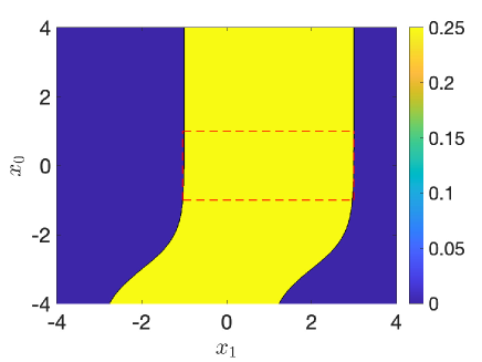
Figure 10: Conditional probability density function $p_{1|0}(x_{1}|x_{0})$ defined in equation (221). The domain $\mathscr{R}(X_{1})\times\mathscr{R}(X_{0})$ is the interior of the rectangle delimited by dashed red lines.

Clearly, the integral of the conditional PDF (221) is

$$\int_{\mathscr{R}(X_{0})}\int_{\mathscr{R}(X_{1})}p_{1|0}(x_{1}|x_{0})dx_{1}dx_{0}=\lambda(\mathscr{R}(X_{0}))=2,$$ (222)

where $\lambda(\mathscr{R}(X_{0}))$ is the Lebesgue measure of $\mathscr{R}(X_{0})=[-1,1]$. The $L^{2}$ norm of the operators $\mathcal{N}$ and $\mathcal{M}$ is bounded by

$$K_{0}= \int_{\mathscr{R}(X_{0})}\int_{\mathscr{R}(X_{1})}p_{1|0}(x_{1}|x_{0})^{2}dx_{1}dx_{0}=\frac{\lambda(\mathscr{R}(X_{0}))}{\lambda(\mathscr{R}(\xi_{0}))}=\frac{1}{2}.$$ (225)

Hence, both operators $\mathcal{N}(1,0)$ and $\mathcal{M}(0,1)$ are contractions (Proposition 17). On the other hand,

$$K_{1}=\frac{\lambda(\mathscr{R}(X_{1}))}{\lambda(\mathscr{R}(\xi_{1}))}=1+\frac{\tan(4)-\tan(2)}{4}>1.$$ (226)

Next, define $V$ as in Lemma 11, i.e., $V=[-3,3]$. Clearly, both $\mathscr{R}(X_{0})$ and $\mathscr{R}(X_{1})$ are subsets of $V$. If we integrate the conditional PDF shown in Figure 10 in $V\times V$ we obtain

$$\int_{V}\int_{V}p_{1|0}(x_{1}|x_{0})^{2}dx_{1}dx_{0}=\frac{\lambda(V)}{\lambda(\mathscr{R}(\xi_{0}))}=\frac{3}{2}.$$ (227)

Operator contractions induced by random noise

In this section, we prove a result on neural networks models (185) which states that it is possible to make both operators $\mathcal{N}$ and $\mathcal{M}$ in (196) contractions if the noise is properly chosen. To this end, we begin with the following lemma.

Lemma 19.

Let $\mathscr{R}(\bm{\xi}_{n})$ and $\mathscr{R}(\bm{\xi}_{n-1})$ be bounded subsets of $\mathbb{R}^{N}$, $\rho_{n}\in L^{2}(\mathscr{R}(\bm{\xi}_{n}))$. If

$$\left\|\rho_{n}\right\|^{2}_{L^{2}(\mathscr{R}(\bm{\xi}_{n}))}\leq\frac{\kappa}{\lambda(\Omega_{n})}\qquad 0\leq\kappa<1$$ (228)

then $\mathcal{M}(n,n+1)$ and $\mathcal{N}(n+1,n)$ are operator contractions. The upper bound in (228) is independent of the neural network weights and biases.

Proof.

The proof follows immediately from equation (212).

∎

Hereafter, we specialize Lemma 19 to neural network perturbed by uniformly distributed random noise.

Proposition 20.

Let $\{\bm{\xi}_{0},\ldots,\bm{\xi}_{L-1}\}$ be independent random vectors. Suppose that the components of each $\bm{\xi}_{n}$ are zero-mean i.i.d. uniform random variables with range $[-b_{n},b_{n}]$ ($b_{n}>0$). If

$$b_{0}\geq\frac{1}{2}\left(\frac{\lambda(\Omega_{0})}{\kappa}\right)^{1/N}\qquad\text{and}\qquad b_{n}\geq\frac{b_{n-1}+1}{\kappa^{1/N}}\qquad n=1,\ldots,L-1,$$ (229)

where $\Omega_{0}$ is the domain of the neural network input, $0\leq\kappa<1$, and $N$ is the number of neurons in each layer, then both operators $\mathcal{M}(n,n+1)$ and $\mathcal{N}(n+1,n)$ defined in (196) are contractions for all $n=0,\ldots,L-1$, i.e., their norm can be bounded by a constant $K_{n}\leq\kappa$, independently of the weights and biases of the neural network.

Proof.

If $\bm{\xi}_{n}$ is uniformly distributed then from (211) it follows that

$$K_{n}=\frac{\lambda\left(\mathscr{R}(\bm{X}_{n})\right)}{\lambda\left(\mathscr{R}(\bm{\xi}_{n})\right)}.$$ (230)

By using Lemma 11 we can bound $K_{n}$ as

$$K_{n}\leq\left(\frac{1+b_{n-1}}{b_{n}}\right)^{N},$$ (231)

where $N$ is the number of neurons in each layer of the neural network. Therefore, if $b_{n}\geq(b_{n-1}+1)/\kappa^{1/N}$ ($n=1,\ldots,L-1$) we have that $K_{n}$ is bounded by a quantity $\kappa$ smaller than one. Regarding $b_{0}$, we notice that

$$K_{0}=\frac{\lambda\left(\mathscr{R}(\bm{X}_{0})\right)}{\lambda\left(\mathscr{R}(\bm{\xi}_{0})\right)}=\frac{\lambda(\Omega_{0})}{(2b_{0})^{N}},$$ (232)

where $\Omega_{0}$ is the domain of the neural network input. Hence, if $b_{0}$ satisfies (229) then $K_{0}\leq\kappa$.

∎

One consequence of Proposition 20 is that the $L^{2}$ norm of the neural network output decays with both the number of layers and the number of neurons if the noise amplitude from one layer to the next increases as in (229). For example, if we represent the input-output map as a sequence of conditional expectations (see (22)), and set $u(\bm{x})=\bm{\alpha}\cdot\bm{x}$ (linear output) then we have

$$q_{L}(\bm{x})=\mathcal{M}(0,1)\mathcal{M}(1,2)\cdots\mathcal{M}(L-1,L)(\bm{\alpha}\cdot\bm{x}).$$ (233)

By iterating the inequalities (229) in Proposition 20 we find that

$$b_{n}\geq\frac{1}{2\kappa^{n/N}}\left(\frac{\lambda(\Omega_{0})}{\kappa}\right)^{1/N}+\sum_{j=1}^{n}\left(\frac{1}{\kappa}\right)^{j/N}\qquad n=0,\ldots,L-1,$$ (234)

In Figure 11 we plot the lower bound at the right hand side of (234) for $\kappa=0.2$ and $\kappa=10^{-4}$ as a function of the number of neurons ($N$).

  $\kappa=0.2$                                                     $\kappa=0.2$

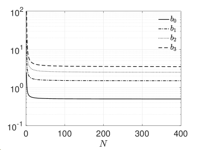
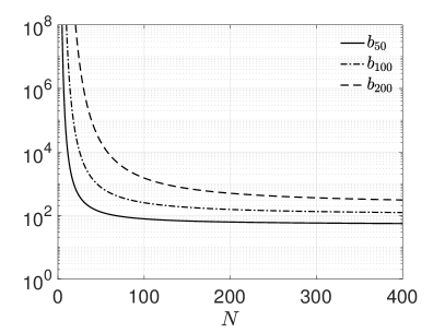
    $\kappa=10^{-4}$                                                    $\kappa=10^{-4}$

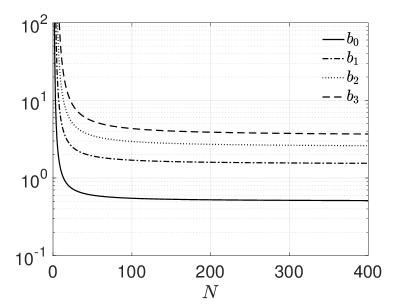
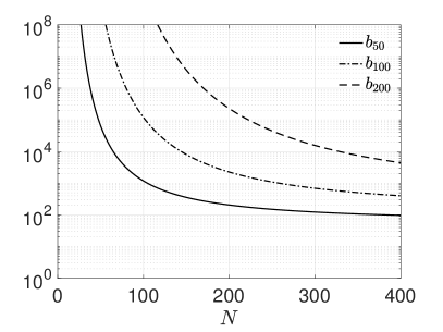
Figure 11: Lower bound on the coefficients $b_{n}$ defined in (234) for $\lambda(\Omega_{0})=1$ as a function of the number of neurons $N$ and the number of layers of the neural network. With such values of $b_{n}$ the operator $\mathcal{M}(n,n+1)$ is a contraction satisfying $\left\|\mathcal{M}(n,n+1)\right\|^{2}\leq\kappa$. Shown are results for $\kappa=0.2$ and $\kappa=10^{-4}$ (contraction index).

With $b_{n}$ given in (234) we have that the operator norms of $\mathcal{M}(n,n+1)$ and $\mathcal{N}(n+1,n)$ ($n=0,\ldots,L-1$) are bounded exactly by $\kappa$ (see Lemma 19). Hence, by taking the $L^{2}$ norm of (233), and recalling that $\left\|\mathcal{M}(n,n+1)\right\|^{2}\leq\kappa$ we obtain

$$\left\|q_{L}\right\|^{2}_{L^{2}(\Omega_{0})}\leq Z^{2}\left\|\bm{\alpha}\right\|^{2}_{2}\kappa^{L},$$ (235)

where

$$Z^{2}=\sum_{k=1}^{N}\int_{\mathscr{R}(\bm{X}_{L})}x_{k}^{2}d\bm{x}\qquad\text{and}\qquad\left\|\bm{\alpha}\right\|^{2}_{2}=\sum_{k=1}^{N}\alpha_{k}^{2}.$$ (237)

The inequality (235) shows that the 2-norm of the vector of weights $\bm{\alpha}$ must increase exponentially fast with the number of layers $L$ if we chose the noise amplitude as in (234). As shown in the following Lemma, the growth rate of $b_{n}$ that guarantees that both $\mathcal{M}$ and $\mathcal{N}$ are contractions is linear (asymptotically with the number of neurons).

Lemma 21.

Under the same assumptions in Proposition 20, in the limit of an infinite number of neurons ($N\rightarrow\infty$), the noise amplitude (234) satisfies

$$\lim_{N\rightarrow\infty}b_{n}=\frac{1}{2}+n,$$ (238)

independently of the contraction factor $\kappa$ and the domain $\Omega_{0}$. This means that for a finite number of neurons the noise amplitude $b_{n}$ that guarantees that $\|\mathcal{M}(n,n+1)\|\leq\kappa$ is bounded from below ($\kappa<1$) or from above ($\kappa>1$) by a function that increases linearly with the number of layers.

Proof.

The proof follows by taking the limit of (234) for $N\rightarrow\infty$. ∎

Appendix B Markovian neural networks

Consider the neural network model (1), hereafter rewritten for convenience

$$\bm{X}_{n+1}=\bm{H}_{n}\left(\bm{X}_{n},\bm{w}_{n},\bm{\xi}_{n}\right)\quad n=0,\ldots,L-1.$$ (239)

In this Appendix we show that if the random vectors $\{\bm{\xi}_{0},\ldots,\bm{\xi}_{L-1}\}$ are statistically independent, and if $\bm{\xi}_{n}$ is independent of past and current states, i.e., $\{\bm{X}_{0},\ldots,\bm{X}_{n}\}$, then (239) defines a Markov process. To this end, we first notice that the full statistical information of the neural network is represented by the joint probability density function of $\{\bm{X}_{L},\ldots,\bm{X}_{0},\bm{\xi}_{L-1},\ldots,\bm{\xi}_{0}\}$. Let us denote by $p\left(\bm{x}_{L},\ldots,\bm{x}_{0},\bm{\xi}_{L-1},\ldots,\bm{\xi}_{0}\right)$ such joint density function. By using well-known identities for conditional PDFs we can write

$$p\left(\bm{x}_{L},\ldots,\bm{x}_{0},\bm{\xi}_{L-1},\ldots,\bm{\xi}_{0}\right)= p\left(\bm{x}_{L}|\bm{x}_{L-1},\ldots,\bm{x}_{0},\bm{\xi}_{L-1},\ldots,\bm{\xi}_{0}\right)\times$$

$$p\left(\bm{x}_{L-1}|\bm{x}_{L-2},\ldots,\bm{x}_{0},\bm{\xi}_{L-1},\ldots,\bm{\xi}_{0}\right)\times\cdots$$

$$p\left(\bm{x}_{0}|,\bm{\xi}_{L-1},\ldots,\bm{\xi}_{0}\right)p\left(\bm{\xi}_{L-1},\ldots,\bm{\xi}_{0}\right).$$ (240)

Clearly, from equation (239) it follows that

$$p\left(\bm{x}_{n+1}|\bm{x}_{n},\ldots,\bm{x}_{0},\bm{\xi}_{L-1},\ldots,\bm{\xi}_{0}\right)=p\left(\bm{x}_{n+1}|\bm{x}_{n},\bm{\xi}_{n}\right).$$ (241)

This allows us to rewrite (240) as

$$p\left(\bm{x}_{L},\ldots,\bm{x}_{0},\bm{\xi}_{L-1},\ldots,\bm{\xi}_{0}\right)= p\left(\bm{x}_{L}|\bm{x}_{L-1},\bm{\xi}_{L-1}\right)p\left(\bm{x}_{L-1}|\bm{x}_{L-2},\bm{\xi}_{L-2}\right)\cdots p\left(\bm{x}_{1}|\bm{x}_{0},\bm{\xi}_{0}\right)p\left(\bm{\xi}_{L-1},\ldots,\bm{\xi}_{0}\right).$$ (242)

If $\{\bm{\xi}_{L_{1}},\ldots,\bm{\xi}_{0}\}$ are statistically independent, and if $\bm{\xi}_{k}$ is independent of $\{\bm{X}_{0},\ldots,\bm{X}_{k}\}$ then

$$p\left(\bm{\xi}_{L-1},\ldots,\bm{\xi}_{0}\right)= p\left(\bm{\xi}_{L-1}\right)\cdots p\left(\bm{\xi}_{0}\right)$$

$$= p\left(\bm{\xi}_{L-1}|\bm{x}_{L-1}\right)\cdots p\left(\bm{\xi}_{0}|\bm{x}_{0}\right).$$ (243)

Substituting (243) into (242) and integrating over $\{\bm{\xi}_{L-1},\ldots,\bm{\xi}_{0}\}$ yields

$$p\left(\bm{x}_{L},\ldots,\bm{x}_{0}\right)= \underbrace{\left(\int p\left(\bm{x}_{L}|\bm{x}_{L-1},\bm{\xi}_{L-1}\right)p\left(\bm{\xi}_{L-1}|\bm{x}_{L-1}\right)d\bm{\xi}_{L-1}\right)}_{p\left(\bm{x}_{L}|\bm{x}_{L-1}\right)}\times\cdots$$

$$\underbrace{\left(\int p\left(\bm{x}_{1}|\bm{x}_{0},\bm{\xi}_{0}\right)p\left(\bm{\xi}_{0}|\bm{x}_{0}\right)d\bm{\xi}_{0}\right)}_{p\left(\bm{x}_{1}|\bm{x}_{0}\right)}p(\bm{x}_{0})$$

$$= p\left(\bm{x}_{L}|\bm{x}_{L-1}\right)p\left(\bm{x}_{L-1}|\bm{x}_{L-2}\right)\cdots p\left(\bm{x}_{1}|\bm{x}_{0}\right)p(\bm{x}_{0}),$$ (244)

which clearly represents the joint PDF of a Markov process. Note that the Markovian property of the process $\{\bm{X}_{n}\}$ representing the neural network states relies heavily on the fact that the joint PDF of the random vectors $\{\bm{\xi}_{L-1},\ldots,\bm{\xi}_{0}\}$ can be factorized as a product of conditional densities as in (243), i.e., that the random vectors are statistically independent, and also that $\bm{\xi}_{n}$ is independent of past and current states, i.e., $\{\bm{X}_{0},\ldots,\bm{X}_{n}\}$.

References

• [1] F. Bartolucci, E. De Vito, L. Rosasco, and S. Vigogna. Understanding neural networks with reproducing kernel Banach spaces. ArXiv:2109.09710, pages 1–42, 2021.
• [2] Z. I. Botev, J. F. Grotowski, and D. P. Kroese. Kernel density estimation via diffusion. Ann. Stat., 38(5):2916–2957, 2010.
• [3] C. Brennan and D. Venturi. Data-driven closures for stochastic dynamical systems. J. Comp. Phys., 372:281–298, 2018.
• [4] H. J. Bungartz and M. Griebel. Sparse grids. Acta Numerica, 13:147–269, 2004.
• [5] M. Chen, X. Li, and C. Liu. Computation of the memory functions in the generalized langevin models for collective dynamics of macromolecules. J. Chem. Phys, 141(6):064112, 2014.
• [6] H. Cho, D. Venturi, and G. E. Karniadakis. Statistical analysis and simulation of random shocks in Burgers equation. Proc. R. Soc. A, 2171(470):1–21, 2014.
• [7] A. J. Chorin, O. H. Hald, and R. Kupferman. Optimal prediction and the Mori–Zwanzig representation of irreversible processes. Proc. Natl. Acad. Sci., 97(7):2968–2973, 2000.
• [8] W. Chu and X. Li. The Mori–Zwanzig formalism for the derivation of a fluctuating heat conduction model from molecular dynamics. Comm. Math. Sci., 17(2), 2019.
• [9] G. Ciccotti and J.-P. Ryckaert. On the derivation of the generalized Langevin equation for interacting Brownian particles. J. Stat. Phys., 26(1):73–82, 1981.
• [10] E. Darve, J. Solomon, and Kia A. Computing generalized Langevin equations and generalized Fokker-Planck equations. Proc. Natl. Acad. Sci., 106(27):10884–10889, 2009.
• [11] A. Dektor, A. Rodgers, and D. Venturi. Rank-adaptive tensor methods for high-dimensional nonlinear pdes. J. Sci. Comput., 88(36):1–27, 2021.
• [12] A. Dektor and D. Venturi. Dynamic tensor approximation of high-dimensional nonlinear PDEs. J. Comput. Phys., 437:110295, 2021.
• [13] J. Dick, F. Y. Kuo, and I. H. Sloan. High-dimensional integration: the quasi-Monte Carlo way. Acta Numer., 22:133–288, 2013.
• [14] J. M. Dominy and D. Venturi. Duality and conditional expectations in the Nakajima-Mori-Zwanzig formulation. J. Math. Phys., 58(8):082701, 2017.
• [15] W. E. A proposal on machine learning via dynamical systems. Commun. Math. Stat., 5:1–10, 2017.
• [16] W. E, J. Han, and Q. Li. A mean-field optimal control formulation of deep learning. Res. Math. Sci., 6:1–41, 2019.
• [17] S. Gibert and A. Mukherjea. Nonnegative idempotent kernels. J. Math. Anal. Appl., 135(1):326–341, 1988.
• [18] L. Gonon, L. Grigoryeva, and J.-P. Ortega. Risk bounds for reservoir computing. JMLR, 21(240):1–61, 2020.
• [19] J. Harlim, S. W. Jiang, S. Liang, and H. Yang. Machine learning for prediction with missing dynamics. J. Comput. Phys., 428:109922, 2021.
• [20] K. He, X. Zhang, S. Ren, and J. Sun. Deep residual learning for image recognition. In Proc. IEEE Comput. Soc. Conf. Comput. Vis. Pattern Recognit., pages 770–778, 2016.
• [21] K. He, X. Zhang, S. Ren, and J. Sun. Identity mappings in deep residual networks. In ECCV, pages 630–645. Springer, 2016.
• [22] J. S. Hesthaven, S. Gottlieb, and D. Gottlieb. Spectral methods for time-dependent problems, volume 21 of Cambridge Monographs on Applied and Computational Mathematics. Cambridge University Press, 2007.
• [23] C. Hijón, P. Español, E. Vanden-Eijnden, and R. Delgado-Buscalioni. Mori–Zwanzig formalism as a practical computational tool. Faraday discussions, 144:301–322, 2010.
• [24] C. Hijón, M. Serrano, and P. Español. Markovian approximation in a coarse-grained description of atomic systems. J. Chem. Phys., 125:204101, 2006.
• [25] S. Izvekov and G. A. Voth. Modeling real dynamics in the coarse-grained representation of condensed phase systems. J. Chem. Phys., 125:151101–151104, 2006.
• [26] G. J. O. Jameson and A. Pinkus. Positive and minimal projections in function spaces. J. Approx. Theory, 37:182–195, 1983.
• [27] D. Kauzlarić, J. T. Meier, P. Español, A. Greiner, and S. Succi. Markovian equations of motion for non-Markovian coarse-graining and properties for graphene blobs. New J. Phys., 15(12):125015, 2013.
• [28] A. I. Khuri. Applications of Dirac’s delta function in statistics. Int. J. Math. Educ. Sci. Technol., 35(2):185–195, 2004.
• [29] Diederik P Kingma and Max Welling. Auto-encoding variational bayes. arXiv preprint arXiv:1312.6114, 2013.
• [30] I. Kobyzev, S. J. D. Prince, and M. A. Brubaker. Normalizing flows: An introduction and review of current methods. IEEE transactions on pattern analysis and machine intelligence, 43(11):3964–3979, 2020.
• [31] A. Lasota and M. C. Mackey. Chaos, fractals and noise: stochastic aspects of dynamics. Springer–Verlag, second edition, 1994.
• [32] H. Lei, N. A. Baker, and X. Li. Data-driven parameterization of the generalized Langevin equation. Proc. Natl. Acad. Sci., 113(50):14183–14188, 2016.
• [33] Q. Li, L. Chen, C. Tai, and W. E. Maximum principle based algorithms for deep learning. JMLR, 18:1–29, 2018.
• [34] Q. Li, T. Lin, and Z. Shen. Deep learning via dynamical systems: An approximation perspective. J. Eur. Math. Soc., (published online first), 2022.
• [35] K. K. Lin and F. Lu. Data-driven model reduction, Wiener projections, and the Koopman-Mori-Zwanzig formalism. J. Comput. Phys., 424:109864, 2021.
• [36] F. Lu, K. Lin, and A. Chorin. Comparison of continuous and discrete-time data-based modeling for hypoelliptic systems. Comm. Appl. Math. Comput. Sci., 11(2):187–216, 2016.
• [37] Y. Lu, Zhong A, Q. Li, and B. Dong. Beyond finite layer neural networks: Bridging deep architectures and numerical differential equations. arXiv:1710.10121, 2017.
• [38] L. Ma, X. Li, and C. Liu. The derivation and approximation of coarse-grained dynamics from Langevin dynamics. J. Chem. Phys., 145(20):204117, 2016.
• [39] Lina Ma, Xiantao Li, and Chun Liu. Coarse-graining langevin dynamics using reduced-order techniques. Journal of Computational Physics, 380:170–190, 2019.
• [40] E. Minguzzi. The equality of mixed partial derivatives under weak differentiability conditions. eal Anal. Exch., 40(1):81–98, 2014/2015.
• [41] H. Mori. Transport, collective motion, and Brownian motion. Prog. Theor. Phys., 33(3):423–455, 1965.
• [42] E. Novak and K. Ritter. Simple cubature formulas with high polynomial exactness. Constr. Approx., 15:499–522, 1999.
• [43] D. Nozaki, D. J. Mar, P. Grigg, and J. J. Collins. Effects of colored noise on stochastic resonance in sensory neurons. Phys. Rev. Lett., 82(11):2402–2405, 1999.
• [44] Sinno Jialin Pan and Qiang Yang. A survey on transfer learning. IEEE Transactions on knowledge and data engineering, 22(10):1345–1359, 2010.
• [45] A. Papoulis. Probability, random variables and stochastic processes. McGraw-Hill, third edition, 1991.
• [46] R. Parhi and R. D. Nowak. Banach space representer theorems for neural networks and ridge splines. JMLR, (22):1–40, 2021.
• [47] Grigorios A Pavliotis. Stochastic processes and applications: diffusion processes, the Fokker-Planck and Langevin equations, volume 60. Springer, 2014.
• [48] J. Price and P. Stinis. Renormalized reduced order models with memory for long time prediction. Multiscale Model. Simul., 17(1):68–91, 2019.
• [49] D. Rezende and S. Mohamed. Variational inference with normalizing flows. In International conference on machine learning, pages 1530–1538. PMLR, 2015.
• [50] T. De Rick, S. Lanthaler, and S. Mishra. On the approximation of functions by tanh neural networks. Acta Numerica, 143:732–750, 2021.
• [51] A. Sherstinsky. Fundamentals of recurrent neural network (RNN) and long short-term memory (LSTM) network. Phys. D: Nonlinear Phenom., 404:132306, 2020.
• [52] E. G. Tabak and E. Vanden-Eijnden. Density estimation by dual ascent of the log-likelihood. Comm. Math. Sci., 8(1):217–233, 2010.
• [53] L. N. Trefethen. Multivariate polynomial approximation in the hypercube. Proceedings of the American Mathematical Society, 145(11):4837–4844, 2017.
• [54] N. Črnjarić-Žic, S. Maćešić, and I. Mezić. Koopman operator spectrum for random dynamical systems. J. Nonlinear Sci., 30:2007–2056, 2020.
• [55] D. Venturi, H. Cho, and G. E. Karniadakis. The Mori-Zwanzig approach to uncertainty quantification. In R. Ghanem, D. Higdon, and H. Owhadi, editors, Handbook of uncertainty quantification. Springer, 2016.
• [56] D. Venturi and G. E. Karniadakis. Convolutionless Nakajima-Zwanzig equations for stochastic analysis in nonlinear dynamical systems. Proc. R. Soc. A, 470(2166):1–20, 2014.
• [57] H. Wang and L. Zhang. Analysis of multivariate Gegenbauer approximation in the hypercube. Adv. Comp. Math., 46(53):1–29, 2020.
• [58] T. Yu, Y. Yang, D. Li, T. Hospedales, and T. Xiang. Simple and effective stochastic neural networks. In Proc. Innov. Appl. Artif. Intell. Conf., volume 35, pages 3252–3260, 2021.
• [59] H. Zhang and Y. Xu. Reproducing kernel banach spaces for machine learning. JMLR, (10):2741–2775, 2009.
• [60] Y. Zhu, J. M. Dominy, and D. Venturi. On the estimation of the Mori-Zwanzig memory integral. J. Math. Phys, 59(10):103501, 2018.
• [61] Y. Zhu and D. Venturi. Faber approximation of the Mori-Zwanzig equation. J. Comp. Phys., 372:694–718, 2018.
• [62] Y. Zhu and D. Venturi. Generalized Langevin equations for systems with local interactions. J. Stat. Phys., 178(5):1217–1247, 2020.
• [63] Y. Zhu and D. Venturi. Hypoellipticity and the Mori-Zwanzig formulation of stochastic differential equations. J. Math. Phys., 62:1035051, 2021.
• [64] R. Zwanzig. Memory effects in irreversible thermodynamics. Phys. Rev., 124(4):983, 1961.