PATE: Property, Amenities, Traffic and Emotions Coming Together for Real Estate Price Prediction

Abstract

Real estate prices have a significant impact on individuals, families, businesses, and governments. The general objective of real estate price prediction is to identify and exploit socioeconomic patterns arising from real estate transactions over multiple aspects, ranging from the property itself to other contributing factors. However, price prediction is a challenging multidimensional problem that involves estimating many characteristics beyond the property itself. In this paper, we use multiple sources of data to evaluate the economic contribution of different socioeconomic characteristics such as surrounding amenities, traffic conditions and social emotions. Our experiments were conducted on $\mathbf{28,550}$ houses in Beijing, China and we rank each characteristic by its importance. Since the use of multi-source information improves the accuracy of predictions, the aforementioned characteristics can be an invaluable resource to assess the economic and social value of real estate. Code and data are available at: https://github.com/IndigoPurple/PATE.

I Introduction

Over the last two decades, models combined with large-scale transaction data have been used by computational social scientists to explain, predict, and even forecast social phenomena. The general aim of real estate price prediction is to identify and exploit socioeconomic patterns emerging in real estate transactions over multiple aspects ranging from the property itself to other factors. We would like to gather variables from different sources and methodological backgrounds to create a model for the purpose of real estate price prediction.

Given the importance of real estate investment to the Chinese economy at 10% of its Gross Domestic Product (GDP) [1], an accurate multi-source model that can predict real estate trends will aid the government and private companies to make better informed decisions. Moreover, this will also benefit individuals who are either looking to lease or purchase property. For tenants, rent represents a major monthly expense and individual buyers will look to maximise their long term return on investment. However, real estate valuation is a multifaceted problem that involves estimating many factors of property such as amenities, proximity to public transport and also social emotions. When it comes to data fusion and model selection, these factors make price prediction even more challenging.

Property prices are traditionally estimated based on value of recently sold properties in a given area  [2] and do not consider factors such as surrounding amenities, traffic conditions, proximity to public transport and also social emotions of the location. More recently, the introduction of new sources of data and methods from the computer vision community [3, 4], such as machine learning [5], have changed traditional methods of property valuation. However, these proprietary systems are heavily dependent on the availability of relevant and updated sales transactions data and fail to take into account the impact of factors such as surrounding amenities, traffic conditions and social emotions on the value of the properties. Although some recent studies incorporate inputs such as infrastructure [6], traffic data [7], reviews [8] and neighborhoods [8, 9, 10, 11, 12, 13], they rely on limited factors and ignore the complex intricacies associated with a multi-source data model.

In this paper, by exploiting the characteristics of the property together with factors like amenities, traffic and emotions in the surroundings we study how multi-source features influence real estate prices. Specifically, we analyze $28,550$ real estate transactions in Beijing, China [14] and provide a multi-modal analysis of the price drivers in play. Our main contributions are as follows:

• Our experiments show that the characteristics from different aspects such as amenities, traffic and emotions have an unexpected economic impact on real estate price.

• We rank multi-modal features according to their importance to the real estate price, which is quantitatively evaluated by the F-score.

• We perform 2 different methods - the linear regression and the XGBoost regression for real estate price prediction. We discover that the use of information from different aspects indeed improves the prediction accuracy of both models.

II related work

Estimating the market value of real estate can be viewed as a regression problem with price per square meter being the dependent variable while the independent variables are characteristics that can help correctly determine the price. Therefore the task can be considered a weighted regression of not only property features [2], historical [15] and neighbourhood prices [16] but also pictures [3, 17]. For example, You et al. [3] created a Recurrent Neural Network (RNN) using the images of sold houses in the neighborhood. Liu et al. [17] combined textual features and external pictures of the sold house to rank and predict the price. Fu et al. [18] ranked houses through point of interests, their popularity and reviews. Apart from the fact that multimedia data such as pictures requires deep learning to extract features, in fact, existing methods [19, 13] show that common regression models (e.g., the linear regression and the XGBoost regression) are sufficient to achieve good performance in the house price prediction task.

Conventionally, real estate companies collect historical transaction data, mortgage records and tax assessments before relating these variables to the physical attributes of the property. While this method produces reasonable estimates for buyers and sellers, it completely ignores the importance of other characteristics of a neighbourhood.

Research has been performed to examine the effect of socioeconomic and environmental factors on real estate prices. Cortright et al. [9] found a positive correlation between housing prices and walkability - Homes located in more walk-able neighbourhoods; those with a mix of common daily shopping and social destinations within a short distance command a price premium over otherwise similar homes in less walkable areas. In urban areas, people prefer to rely on public transport rather than cars. Thus the presence of a developed public transportation system and low traffic [7] in the area can drive up real estate prices. Some researchers also found that intangible qualities of neighbourhoods like a city’s culture [12], perception [20] and design [4] can boost real estate prices. For example, Hristova et al. [12] demonstrates that economic capital alone does not explain urban development. By mining posts from Flickr, a photo-sharing site, the authors suggested that the combination of cultural and economic capital is a better indicator of real estate prices and socio-economic conditions. In their article, Buonanno et al. [20] combined real estate prices and data from a victimization survey to estimate the effect of crime perception on housing prices in Barcelona, Spain. Real estate prices in neighbourhoods that are perceived as less safe than the average for the city are highly discounted. Using vision-based techniques on photos of home exteriors and interiors, Poursaeed et al. [4] developed a model to estimate the luxury level of a property and analysed how this affects the price of real estate. Finally, Boys et al. [21] analysed data from 6 English cities to show how the value of a place is influenced by factors that are not taken into account by conventional economic models. They stated that it is beauty, a sense of local memory and the urban quality of a place that sometimes matter as much or more than connectivity, space and proximity to work. Moreover, their analysis showed that the presence of greenery is not consistently positive as they are normally assumed to be.

However, each of the aforementioned works only take into consideration a very limited number of factors per time and neglect the role played by other characteristics. And although Nadai et al. [13] explored many different factors(e.g. security perception, the proximity of greenery) in a neighbourhood, they are quite simple. In this paper we use multiple sources of data to assess the economic contribution of different characteristics such as surrounding amenities, traffic conditions and also social emotions.

III method

TABLE I: The name and description of multi-source features we collected and extracted for the real estate data.

#	Category	Feature	Description
0	Property	Year	the building year.
1		Elvt	whether there is an elevator in the building.
2		RmNum	the number of bedrooms in the house.
3		HllNum	the number of living and dining rooms in the house.
4		KchNum	the number of kitchens in the house.
5		BthNum	the number of bathrooms in the house.
6		Lat	the latitude of the house.
7		Lng	the longitude of the house.
8	Amenity	TspNum	the number of surrounding transportation infrastructure.
9		TspDst	the average distance of surrounding transportation infrastructure.
10		AtrNum	the number of surrounding tourist attractions.
11		AtrDst	the average distance of surrounding tourist attractions.
12		EdcNum	the number of surrounding education and training institutions.
13		EdcDst	the average distance of education and training institutions.
14		HthNum	the number of surrounding healthcare infrastructure.
15		HthDst	the average distance of surrounding healthcare infrastructure.
16		RstNum	the number of surrounding restaurants.
17		RstDst	the average distance of surrounding restaurants.
18		RtlNum	the number of surrounding retail goods and services.
19		RtlDst	the average distance of surrounding retail goods and services.
20	Traffic	TrfV	the average value of daily traffic speeds.
21	Emotions	AgrPct	the percentage of anger in all emotions.
22		DstPct	the percentage of detestation in all emotions.
23		HppPct	the percentage of happiness in all emotions.
24		SadPct	the percentage of sadness in all emotions.
25		FeaPct	the percentage of fear in all emotions.
26		Price	the price per square meter of the house in Renminbi (RMBa).
aRMB is the legal currency of China.

To provide a multi-source data analysis and thus competently predict the real estate price per square meter, we first perform data collection and pre-processing in Section III-A. After extracting $27$ features from raw data, we compute feature correlations in Section III-B. We then analyze the feature importance to real estate price in Section III-C. Finally, we adopt 2 different methods for real estate price prediction in Section III-D - linear regression and XGBoost regression.

It is worth noting that our objective is to make an attempt to predict real estate prices by combining factors such as property, amenities, traffic and social emotions. Rather than designing and implementing novel prediction methods, we focus on exploring the effectiveness of data fusion and its benefits. As demonstrated in previous work where multi-source data is used for real estate price prediction [13], we adopt the commonly used linear and XGBoost regression as prediction models. Experiment results in Section IV show that these two methods have already achieved feasible performance and sufficiently evaluated the impact of different factors from multi-source data on real estate price.

III-A Data

III-A1 Property

We collect real estate transaction data from the internet and extract features. Specifically, for each real estate transaction, we extract the basic property features such as the building year and the number of bedrooms. In addition, we obtain the its geographical coordinates from the address of the real estate. In total, we get $28,550$ pieces of real estate data with basic property features.

III-A2 Amenities

Since we know the geographical coordinates for each real estate, we can use Baidu Maps to identify surrounding amenities within a kilometer radius. These are further categorized into $5$ types: transportation, tourist attractions, educational institutions, healthcare facilities and restaurants. We compute the total number and average distance of each type of the surrounding amenities as features of the real estate.

III-A3 Traffic

We also use Baidu Maps to obtain traffic information around every real estate. For each real estate property, we collect its surrounding traffic speed information per $5$ minutes from 6 a.m to 12 a.m. We then compute the average traffic speed value as a feature of the real estate, which intuitively reflects the efficiency of transportation surround the real estate.

III-A4 Emotions

We collect microblog posts in Beijing and then use the social emotions analysis algorithm from Ref. [22] to analyze the emotions of each microblog post. Each microblog post is classified as one of the following $5$ types: anger, detest (dislike), happiness, sadness, fear. For each real estate, we calculate the percentage of different emotions related to it as emotions features.

In a total, for every real estate transaction, we extract $27$ features of different aspects, i.e., property, amenities, traffic, emotions from the collected multi-source data. Table I lists the name and description of those extracted features. Since we aim to predict the prices of real estate, we denote the feature Price in Table I as the dependent variable $y$ and the other features as independent variables $x_{i}(i=0,\dots,25)$.

III-B Feature Correlation

Using correlation, we understand the relationship between multiple features. We can use the $r$ value, also called Pearson’s correlation coefficient [23]:

$$r_{uv}=\frac{\sum^{n}_{j=1}(u_{j}-\overline{u})(v_{j}-\overline{v})}{\sqrt{\sum^{n}_{j=1}(u_{j}-\overline{u})^{2}}\sqrt{\sum^{n}_{j=1}(v_{j}-\overline{v})^{2}}},$$ (1)

where $n$ is the sample size; $u_{j}$, $v_{j}$ are the individual sample points indexed with $j$; $\overline{x}$ is the sample mean obtained by $\overline{x}=\frac{1}{n}\sum^{n}_{j=1}x_{j}$; and analogously for $\overline{y}$.

This measures how closely two features are correlated. The $r$ value is a number between $-1$ and $1$. The closer to $1$, the stronger the positive correlation. The closer to $-1$, the stronger the negative correlation (i.e., the more “opposite” the features are). The closer to $0$, the weaker the correlation. We will discuss the experiments and results in Section IV-A.

III-C Feature Importance

Generally, importance provides a score that indicates how useful or valuable each feature is in the construction of the boosted decision trees within the model. The more an attribute is used to make key decisions with decision trees, the higher its relative importance. This importance is calculated explicitly for each feature, allowing features to be ranked and compared to each other. We estimate the importance of different features for real estate price prediction problem using the XGBoost library in Python. We will discuss the experiments and results in Section IV-B.

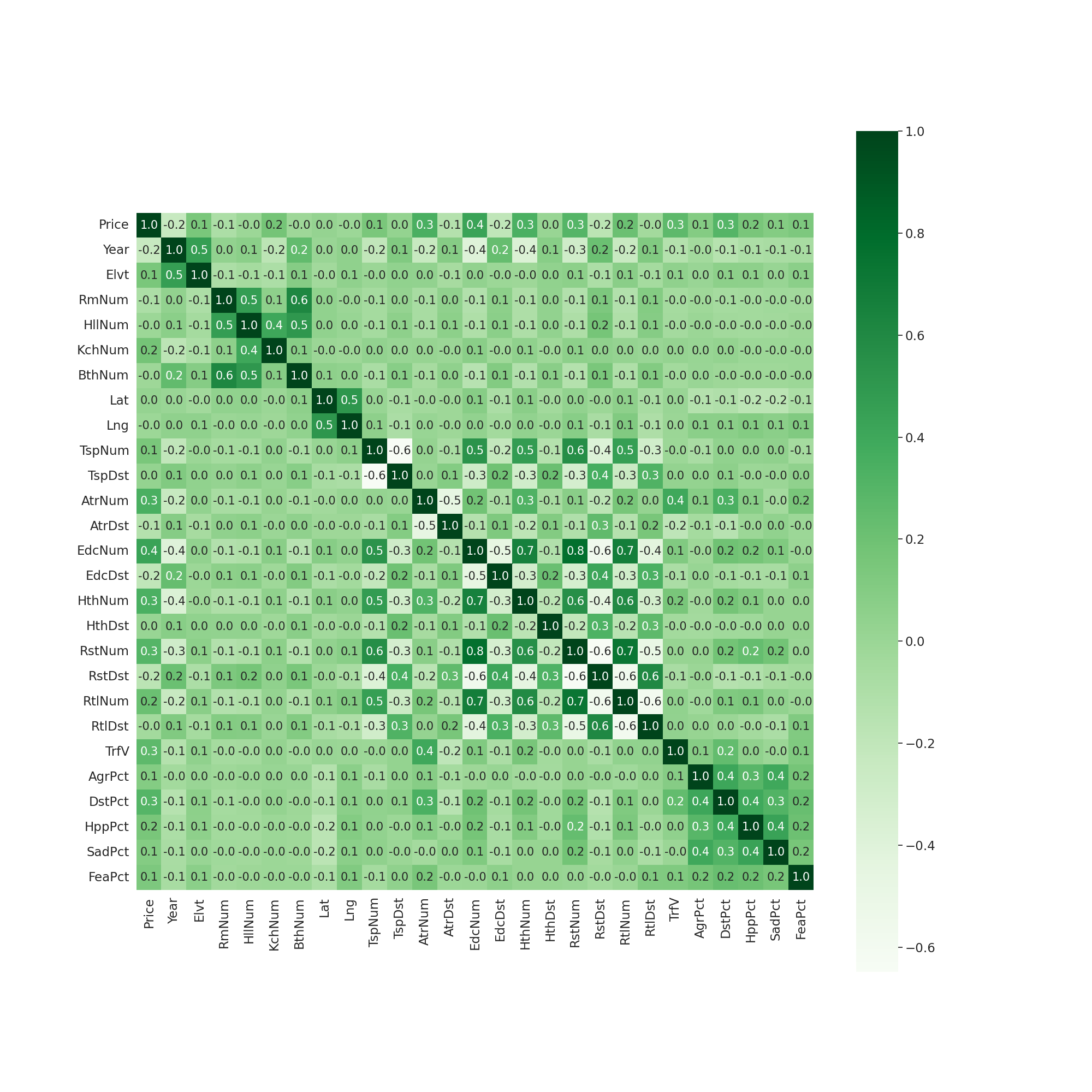
Figure 1: The relationship between multiple features, measured by the $r$ value, also called Pearson’s correlation coefficient [23]. The $r$ value is a number between $-1$ and $1$. The closer to $1$, the stronger the positive correlation. The closer to $-1$, the stronger the negative correlation (i.e., the more “opposite” the features are). The closer to $0$, the weaker the correlation.

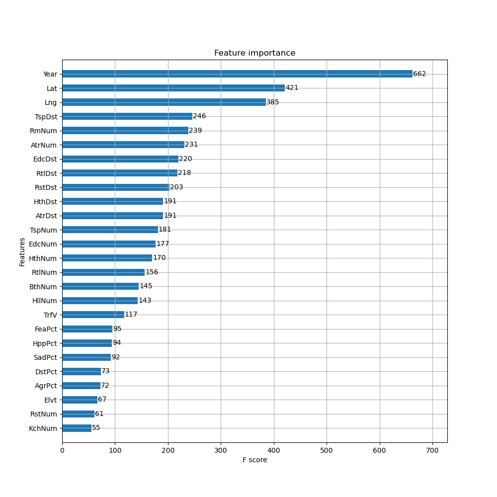
Figure 2: The importance of different features for the real estate price prediction problem estimated with use of the XGBoost library in Python.

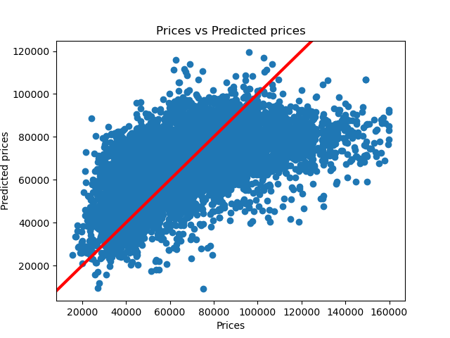
(a)

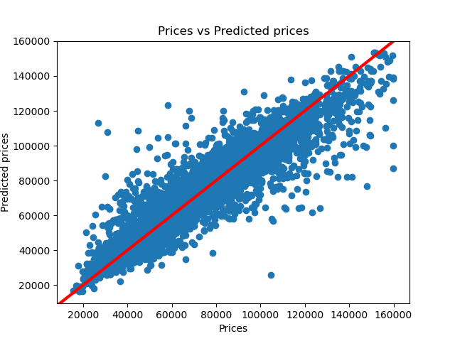
(b)

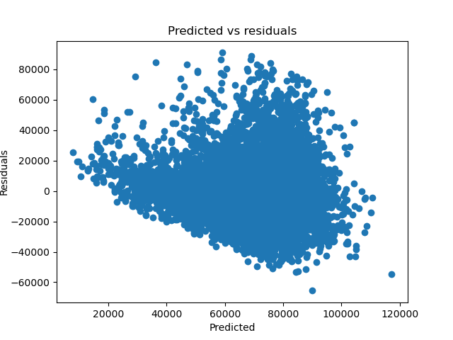
(c)

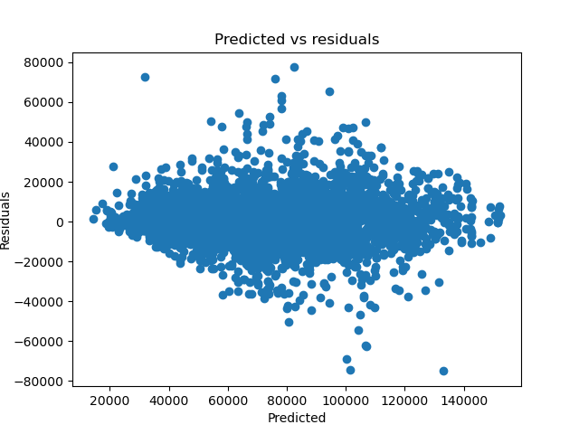
(d)

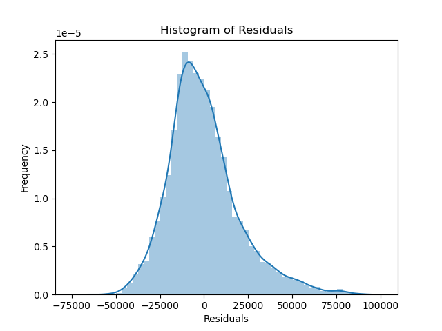
(e)

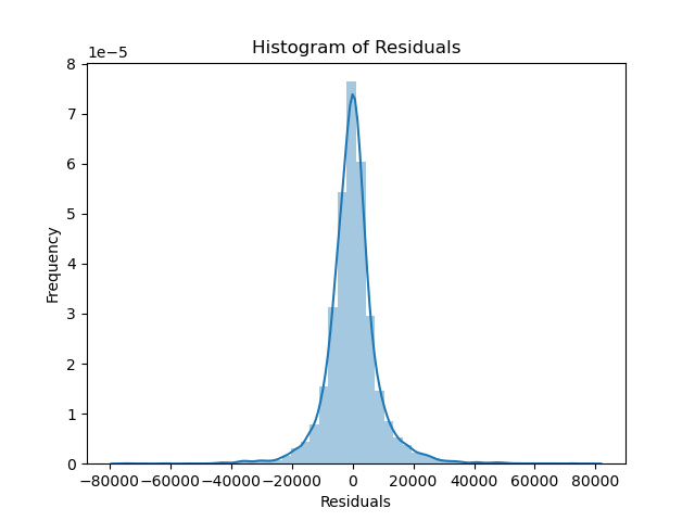
(f)

Figure 3: Intuitive comparisons between the linear and XGBoost regression model for real estate price prediction. (a) The differences between actual prices and predicted values of the linear regression model. The red curve is the $x=y$ line. (b) The differences between actual prices and predicted values of the XGBoost regression model. (c) The residuals of actual prices and predicted values of the linear regression model. (d) The residuals of actual prices and predicted values of the XGBoost regression model. (e) The histogram of errors of the linear regression model. (f) The histogram of errors of the XGBoost regression model.

III-D Prediction Model

Using the complex features from multi-source data, we can build models to predict the real estate price. Specifically, we perform two different methods - the linear regression and the XGBoost regression, since prior works [19, 13] demonstrate that those common regression models are sufficient to yield competent performance in the house price prediction task.

III-D1 Linear Regression

A linear regression model assumes that the relationship between the dependent variable $y$ and the explanatory variables $x_{i}(i=0,\dots,25)$ is linear. Thus the model takes the form:

$$y=\alpha_{0}x_{0}+\alpha_{1}x_{1}+\dots+\alpha_{25}x_{25}+\beta,$$ (2)

where $\alpha_{0},\dots,\alpha_{25}$ are regression coefficients, and $\beta$ is the intercept term.

III-D2 XGBoost Regression

Due to the simplicity and inaccuracy associated with the linear regression model, We additionally perform an advanced algorithm for real estate price prediction. Extreme Gradient Boosting (XGBoost) [24] is an open-source library that provides an efficient and effective implementation of the gradient boosting algorithm. It can be used directly for regression predictive modeling. Therefore, we perform XGBoost regression for advanced prediction modelling.

The loss function of XGBoost is the sum evaluated over all the predictions and a regularization function for all predictors:

$$\mathcal{L}(\theta)=\sum_{j=1}^{n}l(y_{j}-\hat{y}_{j})+\sum_{t=1}^{T}\Omega(f_{t}),$$ (3)

where $n$ is the sample size; $y_{j}$, $\hat{y}_{j}$ are the actual and predicted values of the dependent variable; $T$ is the total number of predictors (trees); $f_{t}$ is the prediction coming from the $t_{th}$ tree.

We will discuss the experiments and results of the aforementioned two different methods in Section IV-C.

III-E Evaluation

We use 5 metrics to measure the accuracy of different models: R-squared ($R^{2}$), adjusted $R^{2}$, mean absolute error (MAE), mean squared error (MSE), root mean squared error (RMSE). Their formulae are as follows:

$$R^{2} =1-\frac{\sum_{j=1}^{n}(y_{j}-\hat{y}_{j})^{2}}{\sum_{j=1}^{n}(y_{j}-\overline{y})^{2}},$$ (4)

$$AdjustedR^{2} =1-[\frac{(1-R^{2})\times(n-1)}{n-k-1}],$$ (5)

$$MAE =\frac{\sum_{j=1}^{n}|y_{j}-\hat{y}_{j}|}{n},$$ (6)

$$MSE =\frac{\sum_{j=1}^{n}(y_{j}-\hat{y}_{j})^{2}}{n},$$ (7)

$$RMSE =\sqrt{\frac{\sum_{j=1}^{n}(y_{j}-\hat{y}_{j})^{2}}{n}},$$ (8)

where $n$ is the sample size; $y_{j}$, $\hat{y}_{j}$ are the actual and predicted values of the dependent variable; $\overline{y}$ is the average of all the actual dependent variable values; $k$ is the number of independent variables in the model, excluding the constant.

TABLE II: The intercept term and regression coefficients of the trained linear regression model.

Intercept	548013.5557669624
#	Feature	Coefficients
0	Year	-225.754
1	Elvt	8321.2
2	RmNum	-2341.1
3	HllNum	-1195.1
4	KchNum	16563.6
5	BthNum	4251.97
6	Lat	10408
7	Lng	-4548.27
8	TspNum	28.063
9	TspDst	25.2256
10	AtrNum	307.328
11	AtrDst	3.91726
12	EdcNum	316.915
13	EdcDst	-10.4586
14	HthNum	150.618
15	HthDst	6.581
16	RstNum	109.195
17	RstDst	15.6027
18	RtlNum	-236.629
19	RtlDst	4.77269
20	TrfV	157.894
21	AgrPct	194.2
22	DstPct	860.433
23	HppPct	33.1033
24	SadPct	35.2334
25	FeaPct	212.4

TABLE III: Experiments with a variety of settings: 1) using only property features, denoted as w/ only P; 2) using property, traffic, emotions features but without amenity features, denoted as w/o A; 3) using property, amenity, emotions features but without traffic features, denoted as w/o T; 4) using property, amenity, traffic features but without emotions features, denoted as w/o S; 5) using all features including property, amenity, traffic, and emotions, denoted as w/ PATE.

Data	Method	$R^{2}$	Adjusted $R^{2}$	MAE	MSE	RMSE
Training set	Linear regression w/ only P	0.1674	0.1671	18284	551713399	23489
	Linear regression w/o A	0.2520	0.2515	16947	495668829	22264
	Linear regression w/o T	0.3730	0.3722	15499	415469247	20383
	Linear regression w/o E	0.3636	0.3629	15582	421702012	20535
	Linear regression w/ PATE	0.3797	0.3789	15391	411032381	20274
	XGBoost regression w/ only P	0.9095	0.9095	5206	59965069	7744
	XGBoost regression w/o A	0.9184	0.9183	4941	54069367	7353
	XGBoost regression w/o T	0.9331	0.9330	4416	44350499	6660
	XGBoost regression w/o E	0.9319	0.9318	4477	45145802	6719
	XGBoost regression w/ PATE	0.9343	0.9342	4387	43549356	6599
Testing set	Linear regression w/ only P	0.1626	0.1618	17905	530648157	23036
	Linear regression w/o A	0.2437	0.2424	16696	479250332	21892
	Linear regression w/o T	0.3591	0.3572	15324	406118449	20152
	Linear regression w/o E	0.3510	0.3494	15358	411213070	20278
	Linear regression w/ PATE	0.3651	0.3632	15235	402302484	20057
	XGBoost regression w/ only P	0.8560	0.8558	6244	91267181	9553
	XGBoost regression w/o A	0.8646	0.8644	6080	85802314	9263
	XGBoost regression w/o T	0.8751	0.8747	5773	79153827	8897
	XGBoost regression w/o E	0.8740	0.8737	5814	79830419	8935
	XGBoost regression w/ PATE	0.8770	0.8766	5721	77956264	8829

IV experiment

IV-A Feature Correlation

As Figure 1 shows, the $r$ value of correlation between the Price and other variables is within the range of $[-0.2,0.4]$ thus indicating that the linear correlation is weak. Therefore, it is unlikely to use only one or few features to accurately predict the real estate price. Rather, it is necessary and effective to collectively gather multiple features of different aspects from multi-source data for accurate prediction.

Besides, considering the correlation to the real estate price, we additionally observe that features within the same category would show a certain correlation. Specifically, we observe some interesting patterns:

1. For the property features, the correlation coefficient on the RmNum and BthNum is $0.6$. In other words, the number of bedrooms in the house and the number of bathrooms have high correlation.

2. For the amenity features, they show a lot of different relationships. For example, the correlation coefficient on the EdcNum and HthNum is $0.7$, on EdcNum and RstNum it is $0.8$ and finally on Rst and RtlNum, it is $0.7$. Those observations indicate that educational institutions often have healthcare facilities and restaurants nearby. Moreover, restaurants and retail goods and services are together in the same area.

3. The traffic feature TrfV shows a relatively strong relationship with the AtrNum. This indicates that vehicular traffic is high in areas with high number of tourist attractions.

The above observations suggest several open questions for future work.

IV-B Feature Importance

Figure 2 ranks the importance of different features by their $F$-scores [25] in the XGBoost model. We could observe that:

1. The building year of the real estate, denoted as Year, i.e., the age of the house is the most important factor for the price.

2. The location of the real estate, represented by its latitude Lat and longitude Lng, is the second most important factor for the price.

3. Among all the amenity-related features, the average distance of surrounding transportation infrastructure TspDst is the most important. This indicates that the transport convenience is an important factor for consumers who are looking to buy real estate.

4. The average value of daily traffic speeds TrfV ranks 18th of all the $26$ features. This indicates that even though TspDst and TrfV are both factors related to traffic convenience, real estate consumers care more about the proximity to public transport and relatively ignore the degree of surrounding traffic congestion.

5. As for the structure of the real estate, the number of bedrooms in the house RmNum has the greatest impact on the price, and far exceeds the impact of other types of rooms (e.g., bathroom, living room and kitchen). The number of kitchens KchNum ranks the last among all features, indicating that consumers usually do not care about the number of kitchens in a house.

6. Another interesting observation is that the number of tourist attractions AtrNum ranks second in the amenity-related features and the sixth in all features thus indicating that the real estate in areas with more tourist attractions would have higher price.

7. As for the social emotions around the real estate, we found that fear, happiness and sadness (i.e. FeaPct, HppPct, SadPct) have greater impact on the price than detest and anger (i.e., DstPct, AgrPct).

IV-C Prediction Model

In total we have $28,550$ pieces of data with a dependent variable $y$ and $26$ independent features $x_{i}(i=0,\dots,25)$ as the dataset. We randomly split the dataset and then use $70\%$ of the data as the training set and the remaining $30\%$ as the testing set. Then we perform two different methods for real estate prediction and discuss their results as follows.

After training, we obtain a trained linear regression model as Table II shows and also a trained XGBoost regression model. For an intuitive comparison of linear and XGBoost regression models, we visualize their results on the testing set in Figure 3 and observe the following:

1. Figure 3a, 3b show the differences between actual prices and predicted values of the linear and XGBoost regression model respectively. While the predicted values of the linear regression model tend to be higher than the actual prices, the data points of the XGBoost model evenly distribute around the $x=y$ line thus demonstrating that the prediction of the XGBoost model is accurate.

2. Figure 3c, 3d show the residuals of actual prices and predicted values of the linear and XGBoost regression model. Values of the XGBoost model are distributed equally around zero while the linear regression model has a lot of obvious outliers especially around the predicted value $=80000$.

3. Figure 3e, 3f shows the histogram of errors of the linear and XGBoost regression model. The residuals are normally distributed for both models. However, the variance of the linear regression errors are larger than that of the XGBoost.

IV-D Ablation Study

To evaluate the impacts of different factors from multi-source data on the real estate price, we observe the performance of the linear and XGBoost regression models on the training and testing datasets.

Specifically, we perform experiments with a variety of settings: 1) using only property features, denoted as w/ only P; 2) using property, traffic, emotions features but without amenity features, denoted as w/o A; 3) using property, amenity, emotions features but without traffic features, denoted as w/o T; 4) using property, amenity, traffic features but without emotions features, denoted as w/o E; 5) using all features including property, amenity, traffic, and emotions, denoted as w/ PATE.

As Table III shows, compared to the w/ only P using only the traditional property features, adding any additional feature (i.e., amenity, traffic, or emotions) could improve the performance. We also observe that: 1) Using all features from different aspects including property, amenity, traffic, and emotions achieves the best performance. 2) Removing the amenity feature leads to the largest performance drop, compared to removing the traffic or emotions. This indicates that the amenity features have a greater impact than the traffic and emotions 3) Removing the traffic feature has a relatively slight impact on the performance. It is reasonable since the traffic feature has only one dimension. However, using the one-dimensional traffic feature still could improve the performance.

V discussion

Taken together, our results clearly show the economic effect of different aspects on real estate price. From our analyses, we may also draw several implications for citizens, local authorities and urban planners, and for real-estate investors:

1. For individuals: Buying property is a significant investment for people. Therefore in addition to characteristics of the house, they should not only take into consideration other facets such as proximity to amenities and public transport but also intangible aspects such as the perception of a city’s culture and security. A model which helps make an informed decision using the above factors will lead to improved quality of life due to improved “walkability” and less traffic and also increase the probability of a significant return on the original investment.

2. For government authorities and urban planners: For government authorities and urban planners: Understanding the importance of different features in real estate price prediction can help planners and local authorities with urban development. For example, from Figure 2 we can interpret that the proximity to amenities and services such as public transport and schools has a positive influence on real estate prices. Therefore infrastructure projects and developing public spaces will help refine certain areas of the city. Additionally, by studying trends in changes to the built environment can help identify negative impacts of gentrification such as forced displacement, a fostering of discriminatory behavior by people in power, and a focus on spaces that exclude low-income individuals and people of color. Data models such as PATE are computational tools that will help analyse cities.

3. For Property developers: Rather than just focusing on the characteristics of houses and apartments such as size, number of bedrooms etc, property developers need to expand their view to include place and surroundings. Ideally, urban planners and developers should work in tandem to achieve a high urban vitality. For example, Figure 2 suggests that people would prefer to live in areas with pedestrian spaces and a variety of establishments in its vicinity. In contrast, areas with few amenities and surrounded by large streets that make pedestrian movements difficult have a low vitality.

VI future work

In this paper, our goal is to make an initial attempt to fuse multi-source data for real estate price prediction. Rather than designing and implementing novel prediction methods, we adopt the commonly used linear and XGBoost regression as prediction models. This paper opens possibilities of future work. We could attempt to further improve the prediction accuracy and also enhance performance by designing complex variants of existing models. To stimulate further research, the data and code are available publicly at: https://github.com/IndigoPurple/PATE. While we aim to use our data to enable positive contributions to real estate price prediction, it can also be used to explore its relevance in other applications such as traffic congestion prediction [26].

VII conclusion

In this work, we have studied the economic impact of multi-aspect characteristics on real estate price. This analysis was formulated as a multi-modal problem where we predict the price of real estate given conditions from multi-source data. We collected and re-processed a large dataset of real estate properties and computed surrounding amenity, traffic, and emotions features. We trained and tested the linear and XGBoost regression algorithms and found that the use of information from different aspects increases the prediction accuracy of the model. Our experiments show that the characteristics from different aspects i.e. amenities, traffic, emotions, have an economic impact on real estate price. We ranked multi-modal features according to their importance to the real estate price.

Based on our observations in Section IV-A, our work suggests several open questions for future work. We hope that this research and released methods can pave the way for novel studies on the previously neglected link between the cost of houses and many other factors.

References

- [1] Gabriela Santos. Should global investors worry about the Chinese company Evergrande? . https://am.jpmorgan.com/us/en/asset-management/adv/insights/market-insights/market-updates/on-the-minds-of-investors/should-global-investors-worry-about-the-chinese-company-evergrande/, 2021. [Online; accessed 2-May-2008].
- [2] Elli Pagourtzi, Vassilis Assimakopoulos, Thomas Hatzichristos, and Nick French. Real estate appraisal: a review of valuation methods. Journal of Property Investment & Finance, 2003.
- [3] Quanzeng You, Ran Pang, Liangliang Cao, and Jiebo Luo. Image-based appraisal of real estate properties. IEEE transactions on multimedia, 19(12):2751–2759, 2017.
- [4] Omid Poursaeed, Tomáš Matera, and Serge Belongie. Vision-based real estate price estimation. Machine Vision and Applications, 29(4):667–676, 2018.
- [5] Stanley McGreal, Alastair Adair, Dylan McBurney, and David Patterson. Neural networks: the prediction of residential values. Journal of Property Valuation and Investment, 1998.
- [6] Yanjie Fu, Hui Xiong, Yong Ge, Zijun Yao, Yu Zheng, and Zhi-Hua Zhou. Exploiting geographic dependencies for real estate appraisal: A mutual perspective of ranking and clustering. In Proceedings of the 20th ACM SIGKDD international conference on Knowledge discovery and data mining, pages 1047–1056, 2014.
- [7] Keith Wardrip. Public transit’s impact on housing costs: a review of the literature. 2011.
- [8] Yanjie Fu, Yong Ge, Yu Zheng, Zijun Yao, Yanchi Liu, Hui Xiong, and Jing Yuan. Sparse real estate ranking with online user reviews and offline moving behaviors. In 2014 IEEE International Conference on Data Mining, pages 120–129. IEEE, 2014.
- [9] Joe Cortright. Walking the walk: How walkability raises home values in US cities. CEOs for Cities, 2009.
- [10] E Washington and E Dourado. The premium for walkable development under land use regulations. SSRN Electron. J, 2018.
- [11] Wenshan Wang, Su Yang, Zhiyuan He, Minjie Wang, Jiulong Zhang, and Weishan Zhang. Urban perception of commercial activeness from satellite images and streetscapes. In Companion Proceedings of the The Web Conference 2018, pages 647–654, 2018.
- [12] Desislava Hristova, Luca M Aiello, and Daniele Quercia. The new urban success: How culture pays. Frontiers in Physics, page 27, 2018.
- [13] Marco De Nadai and Bruno Lepri. The economic value of neighborhoods: Predicting real estate prices from the urban environment. In 2018 IEEE 5th International Conference on Data Science and Advanced Analytics (DSAA), pages 323–330. IEEE, 2018.
- [14] Yaping Zhao, Shuhui Shi, Ramgopal Ravi, Zhongrui Wang, Edmund Y Lam, and Jichang Zhao. H4m: Heterogeneous, multi-source, multi-modal, multi-view and multi-distributional dataset for socioeconomic analytics in case of beijing. In IEEE International Conference on Data Science and Advanced Analytics. IEEE, 2022.
- [15] Fei Tan, Chaoran Cheng, and Zhi Wei. Time-aware latent hierarchical model for predicting house prices. In 2017 IEEE International Conference on Data Mining (ICDM), pages 1111–1116. IEEE, 2017.
- [16] David Hallac, Jure Leskovec, and Stephen Boyd. Network lasso: Clustering and optimization in large graphs. In Proceedings of the 21th ACM SIGKDD international conference on knowledge discovery and data mining, pages 387–396, 2015.
- [17] Xiaobai Liu, Qian Xu, Jingjie Yang, Jacob Thalman, Shuicheng Yan, and Jiebo Luo. Learning multi-instance deep ranking and regression network for visual house appraisal. IEEE Transactions on Knowledge and Data Engineering, 30(8):1496–1506, 2018.
- [18] Yanjie Fu, Guannan Liu, Spiros Papadimitriou, Hui Xiong, Yong Ge, Hengshu Zhu, and Chen Zhu. Real estate ranking via mixed land-use latent models. In Proceedings of the 21th ACM SIGKDD International Conference on Knowledge Discovery and Data Mining, pages 299–308, 2015.
- [19] CH Raga Madhuri, G Anuradha, and M Vani Pujitha. House price prediction using regression techniques: a comparative study. In 2019 International Conference on Smart Structures and Systems (ICSSS), pages 1–5. IEEE, 2019.
- [20] Paolo Buonanno, Daniel Montolio, and Josep Maria Raya-Vílchez. Housing prices and crime perception. Empirical Economics, 45(1):305–321, 2013.
- [21] Nicholas Boys Smith, Alessandro Venerandi, and Kieran Toms. Beyond Location: A Study Into the Links Between Specific Components of the Built Environment and Value. Create Streets, 2017.
- [22] Rui Fan, Jichang Zhao, Yan Chen, and Ke Xu. Anger is more influential than joy: Sentiment correlation in weibo. PloS one, 9(10):e110184, 2014.
- [23] Karl Pearson. Correlation coefficient. In Royal Society Proceedings, volume 58, page 214, 1895.
- [24] Tianqi Chen and Carlos Guestrin. Xgboost: A scalable tree boosting system. In Proceedings of the 22nd acm sigkdd international conference on knowledge discovery and data mining, pages 785–794, 2016.
- [25] Cornelis Joost Van Rijsbergen. The geometry of information retrieval. Cambridge University Press, 2004.
- [26] Bodong Zhou, Jiahui Liu, Songyi Cui, and Yaping Zhao. Large-scale traffic congestion prediction based on multimodal fusion and representation mapping. In IEEE International Conference on Data Science and Advanced Analytics. IEEE, 2022.