EPA Particulate Matter Data - Analyses using Local Control Strategy

Abstract

Statistical Learning methodology for analysis of large collections of cross-sectional observational data can be most effective when the approach used is both Nonparametric and Unsupervised. We illustrate use of our NU Learning approach on 2016 US environmental epidemiology data that we have made freely available. We encourage other researchers to download these data, apply whatever methodology they wish, and contribute to development of a broad-based “consensus view” of potential effects of Secondary Organic Aerosols (volatile organic compounds of predominantly biogenic or anthropogenic origin) within PM_2.5 particulate matter on circulatory and/or respiratory mortality. Our analyses here focus on the question: “Are regions with relatively high air-borne biogenic particulate matter also expected to have relatively high circulatory and/or respiratory mortality?”

Keywords: Nonparametric Unsupervised Learning; Local Control Strategy; Clustering as Matching; Permutation Distributions; Random Forests and Partial Dependence Plots.

1 Introduction

When a researcher downloads a large file of cross-sectional data from the internet, it’s too late to worry about potential deficiencies in the experimental design characteristics of observational data. One could discard some parts of the data to make the remainder “look better”: e.g. look more blocked and/or balanced. But using much less than all of the available data opens a researcher up to potential accusations of “cherry-picking” or having “gardened” the data to get some desired result, Glaeser (2006).

Here we use R-functions from CRAN-packages, R Core Team (2022), that implement a highly adaptive strategy that can robustly “design an analysis” of potentially confounded variables. We apply this approach to the data.frame, pmdata, that is part of the newest Version ($1.4$) of the LocalControlStrategy R-package, Obenchain (2015-2022). This data.frame contains a total of $122$ variables that quantify diverse characteristics of $2,980$ individual US Counties. To form pmdata, we merged EPA data downloaded from https://doi.org/10.5281/zenodo.5713903 with data from CDC Wonder (2017), using fips codes. Our PDF file of R-documentation for pmdata, which can be downloaded from https://CRAN.R-project.org/package=LocalControlStrategy, provides “shortened” names for all $122$ variables as well as any original EPA names and variable descriptions.

Researchers wishing to perform analyses using software other than R can access the CSV data file we have posted on dryad, Young and Obenchain (2022), https://doi.org/10.5061/dryad.63xsj3v58. This CSV file contains only the $25$ variables that we initially considered using in our analyses of the $2,973$ US Counties without any missing values for the $11$ variables listed in Table 1.

Since we accessed CDC Wonder data on April 19, 2022 (more than 19 months after EPA researchers), our “2016” CDC data may not actually be identical to that analyzed in PYE et al. (2021). A more important difference is that our analyses here will focus on CDC “Age Adjusted” rates of Circulatory and/or Respiratory mortality, AACRmort, while published EPA analyses used only CDC “crude” (or raw) mortality rates.

Here, we illustrate use of the LC Strategy R-package to implement the NU Learning approach of Obenchain (2015-2022). Its three key-characteristics are:

[a] Users must specify both a single $y-$outcome variable and a single primary (potentially causal) variable that represents either (1) a binary “treatment choice”, $t=0$ or $t=1$, or else (2) a continuous primary “exposure” measure, $e$. The analyses illustrated here use $y=AACRmort$ and $e=Bvoc$ (biogenic volatile organic compounds), which are two of the eleven variables described in Table $1$.

[b] LC Strategy then starts by forming Clusters of observational units (here, US Counties) that are relatively well-matched in an $X-$covariate space also specified by the analyst. Software supporting application of LC Strategy needs to provide statistical measures and graphics that help users make well-informed choices among both clustering algorithms and the best number, $K$, of clusters to use with each algorithm.

[c] The primary output from LC Strategy for each clustering algorithm consists of two new variables: a cluster ID value for each unit, and a local (within cluster) “effect-size” measure for each unit. In our final “Reveal Phase” of LC Strategy, we will illustrate use of Local Rank Correlations (LRCs) between $AACRmort$ and $Bvoc$ within $K=50$ Clusters formed using the ward.D algorithm.

A good place to start our analyses is provided by Figure 1. This scatter plot displays $e=Bvoc$ ($\mu{g}/m^{3}$) from EPA models using satellite data (on the horizontal axis) verses $y=AACRmort$ estimates from the CDC for $2,973$ US Counties. The $Bvoc$ component of PM_2.5 consists of volatile organic compounds that are primarily biogenic (rather than anthropogenic) in origin within “Secondary Organic Aerosols”, Pye et al. (2021). $AACRmort$ values are “Age Adjusted Circulatory and/or Respiratory mortality” counts of deaths per 100,000 residents.

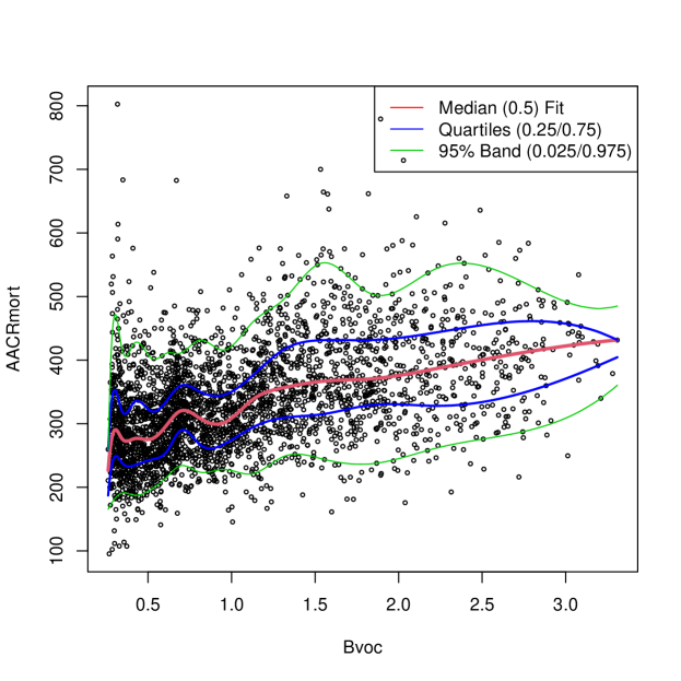
Figure 1: The above scatter for 2,973 US Counties within the contiguous 48 States plus Washington DC reveals considerable variability in $y=AACRmort$ for any given value of $e=Bvoc$. The five (red, blue or green) regression quantiles fitted using the quantreg $R-$package, Koenker (2005-2022), display considerable non-linearity. Thus, given only the Bvoc level of an otherwise unspecified US County, it would clearly be unrealistic to expect a meaningful point-prediction of its AACRmort count to result.

In natural products research, it is standard practice to examine fractions of raw natural material to figure out where an “active agent” is located. There typically are many fewer compounds in the active fraction, so chemical identification becomes more feasible. Starting in 1993, evidence pointing to particulate matter smaller than $2.5$ microns, thereafter known as PM_2.5, became the proposed active fraction in the 1952 London Fog death event, Logan (1953).

In reality, PM_2.5 is a complex mixture of over four thousand chemical compounds which vary over both time and space (urban vs. rural, etc.) PYE et al. (2021) appear to have followed a natural products strategy by arguing that “Secondary Organic Aerosols” (SOAs) could be “the” active agents in PM_2.5. Unfortunately, in the almost 30 years since PM_2.5 publications sponsored by the US EPA first appeared, neither measures of PM_2.5 itself, nor any fraction of it, has been convincingly shown to be genuinely predictive of mortality at the level of individual US Counties and Cities.

Young, Kindzierski and Randall (2021) suggest that the current EPA paradigm that “PM_2.5 is, by itself, lethal” is wrong. While the efforts of Pye et al. (2021) may be noble, potential challenges to their proposals abound.

2 Predicted rather than Observed Measures of SOAs

Although actual measurements of SOA components in air samples are apparently not currently feasible, various “models” for predicting their presence from measurements of other pollutants have apparently been used since Volkamer et al. (2006). The analyses presented in Pye et al. (2021) appear to be based upon the EPA’s Community Multiscale Air Quality (CMAQ) System Models, U.S. EPA Office of Research and Development (2019). Unfortunately, neither the assumptions nor any limitations of those models are discussed in Pye et al. (2021).

For example, a potential issue is that CMAQ may be loosely based upon Generalized Additive Model (GAM) concepts. While Pye et al. (2021) do reference Wood (2003, 2004 and 2022), their introduction claims that they use “multiple linear regression”, a methodology that makes strong and seemingly unrealistic assumptions for observational data. Since GAMs are a composite of several individual models, some sub-models could be fit in unspecified “non-standard” ways. All that we know as outside observers is that these EPA models do a much better job of predicting CDC measures of Circulatory and/or Respiratory mortality (raw or age-adjusted) than we would have expected. In short, we would much rather have had actual observed measurements of secondary organic aerosols from validated scientific instruments to analyze here …and to make available to other researchers.

3 Variables of Primary Interest within CDC and EPA Data

There are $25$ variables (columns) and $2,973$ observations (rows) in the “AnalysisFile.csv” file that we have archived at dryad, Young and Obenchain (2022), while the analyses presented here actually use only the $11-$variables described in Table $1$. Six US Counties out of the original $2,980$ had NA codes on the rather important PREMdeath variable (fips = 8033, 30055, 31091, 46069, 46073 and 49031), while a $7^{th}$ NA code occurred for fips = 32011 in the IncomIEQ variable, which turned out to be a relatively unimportant confounder.

The analyses presented here will ultimately focus on “potential causes” of Circulatory and Respiratory Mortality within individual US Counties. Our focus on the AACRmort variable from the CDC (rather than CRmort) stems primarily from our previous experience [Obenchain, Young and Krstic (2019)] where the proportion of county residents over 65 was a key predictor of local mortality. While we did perform some preliminary analyses using CRmort as the primary $y-$Outcome, we found them to be both more complex and less self-consistent than the corresponding AACRmort analyses that we present here.

Our somewhat surprising and unexpected findings concerning distinct components of pmTOT (i.e. PM_2.5) focus primarily upon Bvoc, although the Avoc and pmSO4 levels from the EPA are among the confounders considered in our final analyses.

TABLE 1 – Variable Information
Name	Description	Range
fips	Federal Information Processing code ($4$ or $5$ digits)	1001-56045
CRmort	Circulatory/Respiratory (crude) mortality (per 100K)	64.8-1564
AACRmort	Age Adjusted Circulatory/Respiratory mortality (per 100K)	95.5-802.6
pmTOT	Observed $PM_{2.5}$ level ($\mu$g/m3)	2.06-14.32
Bvoc	Biogenic volatile organic compounds in pmTOT	0.26-3.31
Avoc	Anthropogenic volatile organic compounds in pmTOT	0.23-2.89
pmSO4	Sulfate compounds in pmTOT	0.39-1.62
ASmoke	Adult Smoking fraction	0.007-0.412
PREMdeath	Premature Death rate	0.03-0.66
ChildPOV	Children living in Poverty (per 100K)	2853-36469
IncomIEQ	Income In-Equality rating	2.9-8.9

Although we ultimately focus on Local (within Cluster) models that are highly-flexible and statistically robust, we initially used multiple linear regression to assess the “overall” extent of ill-conditioning (confounding) among variables; see Figure 2. This Trace display shows fitted regression coefficients on the Efficient Generalized Ridge Regression shrinkage path, Obenchain (2005-2022). This linear model attempts to predict $AACRmort$ using $Bvoc$, $Avoc$, $pmSO4$, $PREMdeath$, $ASmoke$, $ChildPOV$ and $IncomIEQ$. While the order in which these seven “right-hand-side” variables are specified is irrelevant in classical linear regression, the first three are EPA environmental variables while the last four (hopefully) quantify socioeconomic characteristics of county residents.

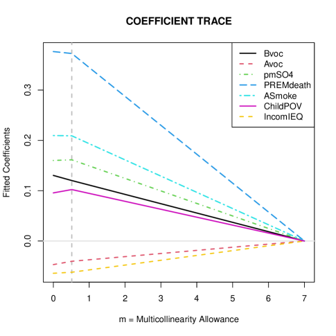
Figure 2: Following a modest initial extent of shrinkage to $m=0.51$, MSE-risk optimal relative-magnitudes for $\beta-$coefficient estimates are determined, Obenchain (2022). In other words, overall ill-conditioning (redundancy) among these seven $X-$variables appears minor. Since our main LC Strategy analyses will use AACRmort as the $y-$Outcome measure, we will focus on Bvoc as our primary (potentially causal) Exposure variable. After all, the EPA Avoc and IncomIEQ variables have only small and negative coefficient estimates. The overall $R^{2}-$Coefficient of Determination for this linear model is not particularly high (coincidentally, also $0.51$). Thus, true relationships here could be nonlinear. In fact, the “local” models developed here will be distribution-free and correspond to much better fits.

4 Applying Local Control Strategy

LC Strategy consists of Four Phases of analysis called, respectively : Aggregate, Confirm, Explore and Reveal. Each analysis “cycle” through the available data typically uses a different Aggregation of observational units into a larger and larger number, $K$, of smaller and smaller “Clusters”. Potential results from each new cycle are ultimately Discarded unless they have been Confirmed to provide Added Information …in the sense of being clearly different from “purely random” in ways outlined below.

The implicit statistical model used in LC Strategy is a simple “one-way” classification of within-cluster estimates. In the analyses presented here, these estimates are “Local Rank Correlations” (Spearman LRCs) between an Exposure e-variable and an Outcome y-variable, both of which are potentially continuous measures …i.e. have many more than just two levels. Specifically, we discuss the special case where the $e-$variable is Bvoc and the $y-$outcome measure is AACRmort. Thus, when the $j^{th}$ cluster contains $N_{j}$ US Counties, $N_{j}$ identical LRC estimates are contributed to the overall (across cluster) distribution of LRC Effect-Sizes.

Note, in particular, that analyses focused on LRC estimates implement a variation on the recommendation of Rubin (2008) for analysts to be “blinded” to the numerical values of the y-outcome ($AACRmort$) and primary exposure ($Bvoc$) variables. Specifically, the $LRC$ vector of values created via LC Strategy guides all subsequent primary analyses. Clusters with $LRC$ estimates near zero suggest “absence of any clear local relationship” between $Bvoc$ and $AACRmort$, while strongly non-zero $LRCs$ suggest local relationships that tend to be nearly monotone increasing or decreasing between $Bvoc$ and $AACRmort$ within that particular cluster.

While LC Strategy can be used by single researchers working alone, this strategy can also be used by a group of collaborating researchers. In fact, LC Strategy may be an ideal approach when the researches involved in a collaboration have “odd combinations” of qualifications …such as: diverse experiences and unique perspectives on the overall issues involved. Use of LC Strategy plus access to relevant data then makes it possible to seriously address the question: Can any shared, consensus position be reached?

Our discussion of LC Strategy below will use the basic terminology outlined in Table $2$.

TABLE 2 – Basic LC Strategy Terminology
Term	Description
Observational Unit	An individual US County or Parish within the contiguous 48 States
	or the District of Columbia.
Cluster	A subgroup of Units that are relatively well-matched on their given
	$X-$characteristics.
Cycle	One “pass” through the data involving at least the Aggregate and
	Explore phases of analysis.
Aggregate	The Phase of LC Strategy where a new set of Clusters are formed.
Confirm	The Phase where a given Aggregation can be shown to either be
	“Ignorable” or to provide Added Information.
Explore	The Phase where Aggregations are compared on Variance-Bias Trade
	Offs and a decision to either Continue or Stop Cycling is made.
Reveal	The final Phase of LC Strategy where the Distribution of Within
	Cluster Local Rank Correlations is analyzed using randomForest()
	functions and Partial Dependence plots.

4.1 Forming a Hierarchical Clustering Tree

The very first step in applying LC Strategy is to form a hierarchical clustering dendrogram. The LocalControlStrategy::LCcluster() function calls stats::prcomp() to calculate Mahalanobis distances using standardized and orthogonal Principal Coordinates, Obenchain (1971) and Rubin (1980). These coordinates optimally quantify “dissimilarity” among US Counties using their possibly confounded $x-$characteristics. A dendrogram (tree-like structure) can usually be “cut” by a horizontal line to produce any desired number of individual clusters. Our example dendrogram, displayed in Figure 3, uses the default “ward.D” clustering algorithm.

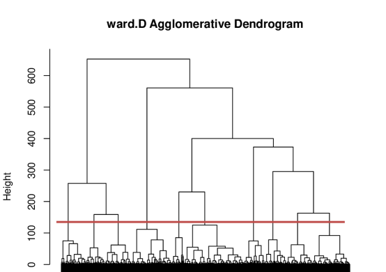
Figure 3: This Hierarchical Clustering Dendrogram can be “cut” by a horizontal line at any strictly positive Height. For example, note that the displayed red line produces 10 clusters.

Either the divisive cluster::diana() method or any of six agglomerative alternatives (ward.D2, complete, average, mcquitty, median, or centroid) could have been specified. However, “single-linkage” clustering is not appropriate for use in LC Strategy because it can produce clusters that are more like “strings” than like compact subgroups of most similar observational units.

4.2 Confirming that a given Number of Clusters provide “Added Information”

Each new Aggregate Phase of LC Strategy may be followed by a full or partial Confirm Phase analysis of the new distribution of within-cluster Local (Spearman) Rank Correlations (LRCs). Each new Clustering provides Added Information if, and only if, the empirical Cumulative Distribution Function (eCDF) of it’s LRC-distribution is clearly different from the NULL eCDF that corresponds to Purely Random assignments of all observational units to the same number, “K”, of Clusters of the exactly same size as the given clusters. This NULL distribution and a two-sample Kolmogorov-Smirnov D-statistic can be efficiently computed (in about 5 seconds) using Random Permutations. A numerically large D-statistic provides only partial confirmation.

Unfortunately, the tabulated distribution of KS D-statistics assumes that both distributions are absolutely continuous, while LRC-distributions are clearly discrete. Thus, LC Strategy uses a (computationally intensive) permutation test, Welch (1990), that is non-parametric. Simulating the $p-$value of an observed LRC $D-$statistic uses the KSperm() function in the LocalControlStrategy $R-$package and typically requires an additional 75 seconds of computation to (potentially) achieve full statistical confirmation “adjusted for Ties”.

Figure 4 displays the numerical example with $K=50$ Clusters that we will use to illustrate confirm phase testing. We are “jumping the gun” here in the sense that we will argue next (in Subsection $4.3$) that $K=50$ is also the “optimal” number of Clusters to use in applying our LC Strategy for NU Learning.

Note that the gray NULL eCDF appears to be rather smooth in Figure 4. After all, it results from pooling $100$ sets of LRC estimates from $50$ pseudo-clusters that were formed in a purely random and meaningless way. Thus the gray eCDF contains at most $5,000$ quite small steps. To truly provide “added information”, the distribution underlying the Blue eCDF from clusters of “well matched” US Counties must be clearly different from the purely random distribution (from random pseudo-clusters) represented by the gray eCDF.

Figure 5 displays the NULL distribution where the largest observed NULL D-statistic is only $0.237$. This simulated NULL D-statistic is dwarfed by the Observed $D-$statistic of $0.7835$ in Figure 4. In other words, the Blue empirical CDF variable, named “LRC50”, provides abundant Added Information in the sense that it is clearly “shifted to the left” in Figure 4 relative to the simulated gray NULL eCDF. The Blue eCDF is thus Not Ignorable! Furthermore, note that some Local Rank Correlation estimates from $K=50$ clusters are clearly negative.

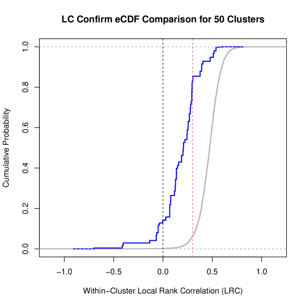
Figure 4: This plot displays a pair of empirical Cumulative Distribution Functions (eCDFs) and addresses the question of whether they are statistically different. Note that the Kolmogorov-Smirnov D-statistic of $0.7835$ (maximum vertical separation between eCDFs) occurs here at $0.30$ on the horizontal axis …marked by the dashed red line.

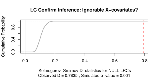
Figure 5: Since the traditional Kolmogorov-Smirnov test compares eCDFs from a pair of Continuous Distributions, it is severely biased when used to compare Discrete Distributions. Thus, simulation is used in LC Strategy to make valid comparisons between eCDF estimates. Since the largest observed NULL D-statistic was only $0.237$, the Observed D of $0.7835$ almost surely has an actual $p-$Value of much less than $0.001$ (one in a thousand).

4.3 Choosing the Number of Clusters to Use in LC Strategy

Especially when cross-sectional data are observational, the data typically contain isolated “local” effects as well as overall (global) confounding from potentially highly correlated variables. The Nonparametric and Unsupervised “pre-processing” methods that characterize LC Strategy address these issues. Traditional methods based on multiple regression are typically Global, Parametric and Supervised. They tend to make much stronger (and possibly unrealistic) assumptions that yield questionable global predictions and potential extrapolations.

In sharp contrast, LC Strategy summarizes findings from several separate and flexible “local” models that are fit within clusters of “most similar” and/or relatively “well-matched” observational units. The number of such local models and separate clusters of observational units being used in a given Cycle is denoted by the symbol K.

LC Strategy embraces many of the basic concepts and experiences outlined in Rubin (2008), Stuart (2010), van der Laan and Rose (2010) and Stang et al. (2010). Published analyses using LC Strategy include: Obenchain and Young (2013); Lopiano, Obenchain and Young(2014); Young, Smith and Lopiano (2017) and Obenchain, Young and Krstic (2019).

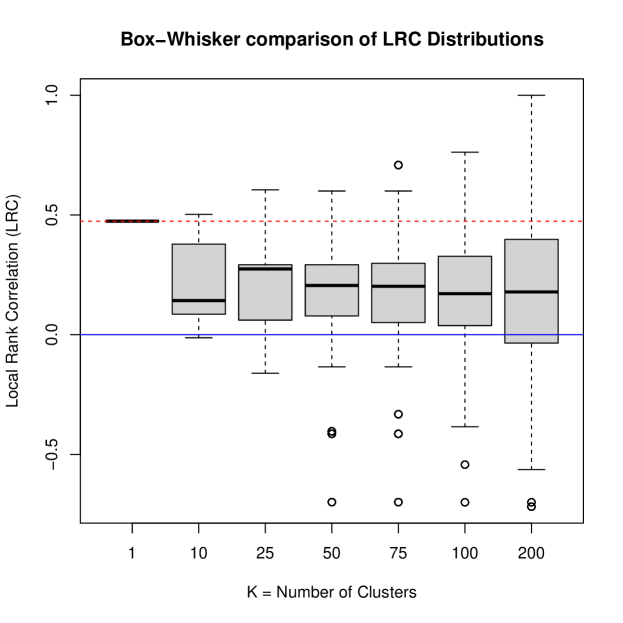
Figure 6: Here we see $7$ alternative Box and Whisker diagrams that show how the overall distribution of LRC effect-sizes changes as the number of clusters, $K$, being formed increases from $1$ to $200$. Note that the LRC distribution for $K=50$ has the smallest interquartile range for $K>1$ as well as shorter whiskers (both upwards and downwards) than the LRC distributions for $K>50$. Our recommended “compromise” choice is thus $K=50$.

Ultimately, we chose to use $K=50$ Clusters of US Counties formed using only the six key $x-$Confounder variables that made (potentially causal) “common sense” to us and repeatedly proved useful in many alternative LC analyses. The resulting $50$ clusters represent mutually exclusive and exhaustive statistical “Blocks” of relatively well-matched observational units, and our resulting “best” Effect-Size distribution quantifies a potentially causal relationship between the numeric $y-$Outcome variable AACRmort and our $e-$Exposure variable Bvoc.

Our choice of $K=50$ clusters was determined within the Explore phase when $Box-Whisker$ plots showed that the distribution of estimated “effect sizes” would become excessively variable for $K>50$. Specifically, any analyst applying LC Strategy would examine the “LCcompare()” graphic displayed in Figure 6 and choose $K=50$ for the very reasons outlined in the caption of that figure. Figure 7 displays a histogram showing variation in the sizes of these $50$ clusters. Finally, Figure 8 shows that the distribution of LRC estimates looks somewhat discrete simply because it contains only $50$ distinct numerical values.

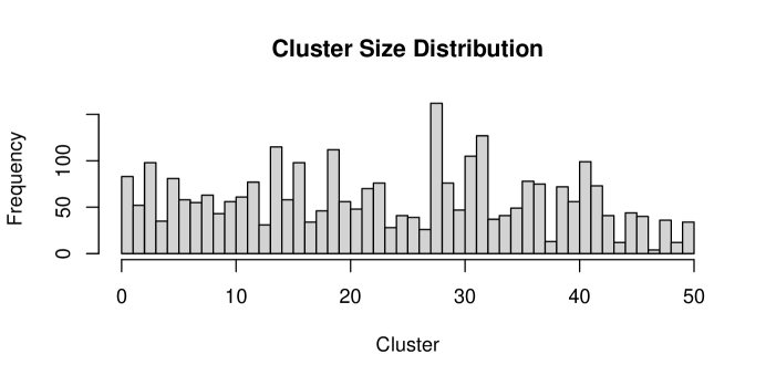
Figure 7: This histogram shows the number of US Counties within each of the 50 Clusters formed using observational data from the EPA, CDC and US Census. In a prospective study (e.g. a well “designed” experiment), all “blocks” of well-matched units are usually of nearly equal size. But that’s an unlikely “ideal” situation when analyses must rely on observational data. The largest cluster contains 162 US Counties, while the smallest contains only four.

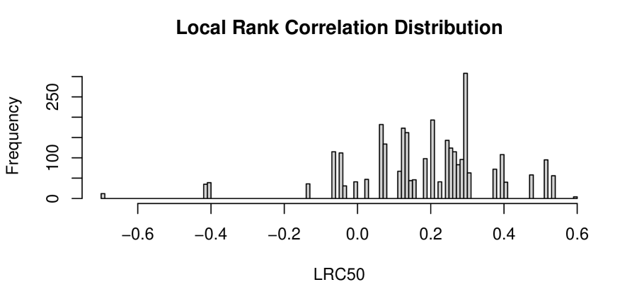
Figure 8: Here we see that the distribution of Local Rank Correlations (LRCs) within our 50 Clusters spans the range from $-0.699$ to $+0.600$. Since this distribution contains only $50$ distinct numerical values, it certainly does not (and cannot) look much like a “continuous” parametric distribution.

5 LC “Reveal” Stage: randomForests, Partial Dependence Plots and a Single RP Tree

We can now stop “Exploring” and enter the (final) “Reveal” phase of NU Learning. Specifically, we now look across, rather than only within, our $K=50$ clusters of relatively well-matched US Counties that provide the most (potentially causal) Added Information about relationships between the AACRmort and Bvoc “measures” of mortality and air pollution, respectively. This new information is embedded within the LRC50 variable that takes on only one of $50$ distinct numerical values between $-0.699$ and $+0.600$ for each US County and is displayed in Figure 8.

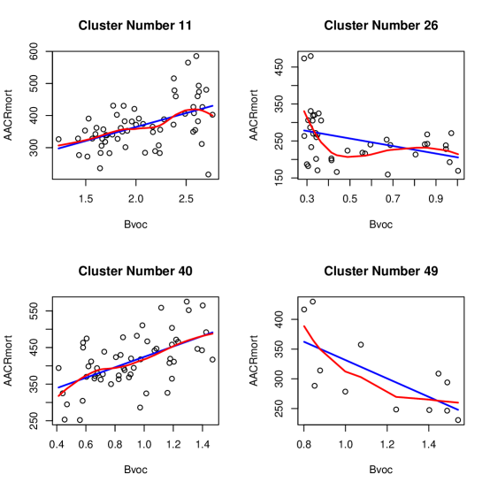
Figure 9: Here are plots of Bvoc versus AACRmort within four of the $50$ Clusters. The straight blue lines are least-squares fits, while the red curves are “loess” smooths (span = $0.75$) for predicting AACRmort from Bvoc. While the (Spearman) LRCs within the two left-hand Clusters ($11$ and $40$) are positive, both right-hand clusters ($26$ and $49$) are typical of the negative LRC estimates observed for a total of $421$ US Counties ($21.3\%$ of the $2,973$ US Counties without missing data).

5.1 Interaction Effects Abound

Figure 9 contains plots of Bvoc versus AACRmort for $4$ of our $50$ Clusters. The two left-hand clusters have positive LRC-estimates and blue least-squares lines that slope upwards, while the two right-hand clusters have negative LRC-estimates and blue least-squares lines that slope downwards. Actually, $421$ US Counties ($21.3\%$) of all $2,973$ US Counties without missing data fall into the $10$ out of $50$ Clusters (i.e. $20\%$) that yield negative LRC-estimates. In other words, almost $80\%$ of US Counties are in the $80\%$ of Clusters with strictly positive LRC-estimates. After all, the Rank-Correlation for the overall Bvoc vs. AACRmort scatter displayed in Figure 1 is $+0.474$. This made us wonder whether larger clusters might tend to produce positive LRC estimates?

An extreme illustration of this is displayed in the lower-right panel of Figure 10. Data from the $237$ Counties within the $6$ clusters with the most Negative LRCs are merged together there, yielding a scatter with clearly positive slope (and an LRC of $+0.267$.) Meanwhile, each of the other $3$ panels shows scatters for only $2$ out of these $6$ clusters with most negative LRCs. Clearly, clustering of US Counties on their confounded $X-$characteristics predictive of AACRmort truly does matter!

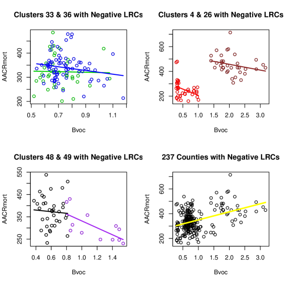
Figure 10: When AACRmort and Bvoc data from the 6 clusters with most Negative LRC estimates are merged together, all other information about differences between these US Counties is discarded. In the lower-right panel, we see that their “Merged Trend” becomes clearly positive …shown in Yellow. Each of the other three panels show AACRmort vs. Bvoc scatters for only two of the six clusters with negative LRCs …using Brown and Red, Blue and Green, or Purple and Black points and “Local Trend” lines.

5.2 Insights from a randomForest of 500 Trees

Given a random forest of $500$ tree models for prediction of LRC estimates [Breiman (2001,2002), Liaw and Wiener (2002 - 2022)], the Partial Dependence Plot (PDP), Friedman (2001), for one potential predictor depicts the marginal relationship that results from averaging over all other potential predictors. This marginal relationship ignores potential interaction effects and can be linear, monotonic or more complex.

The highly detailed captions for the next eight Figures (11 through 18) outline our interpretations of these marginal relationships.

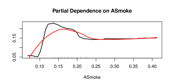
Figure 11: The single most important predictor of LRCs is the local Adult Smoking rate (ASmoke): $\%$IncMSE$=71.28$. ASmoke rates within the $0.15$ to $0.20$ range are predictive of highly positive LRCs between AACRmort and Bvoc. This marginal relationship is not monotone; ASmoke rates above $.25$ correspond to somewhat lower but still relatively high LRCs.

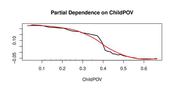
Figure 12: The second most important predictor of LRCs is ChildPOV: $\%$IncMSE$=59.46$. When Child Poverty rates are less than $.30$, LRCs are strongly positive. However, LRCs monotonically decrease and can even become negative when ChildPOV exceed $0.50$. In fact, the ChildPOV fate is the only predictor associated with strictly negative LRC predictions.

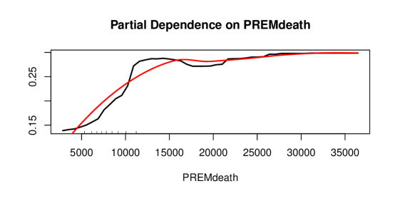
Figure 13: The third most important predictor of LRCs is PREMdeath: $\%$IncMSE$=56.31$. PREMdeath is expressed as a count of “premature deaths” per $100,000$ county residents. As this rate increases from $5,000$ to $15,000$, LRCs steadily increase from $0.15$ to about $0.28$. This marginal relationship is rather close to being monotone increasing. Like ASmoke, PREMdeath appears to be a key determinant of excess Circulatory and/or Respiratory mortality.

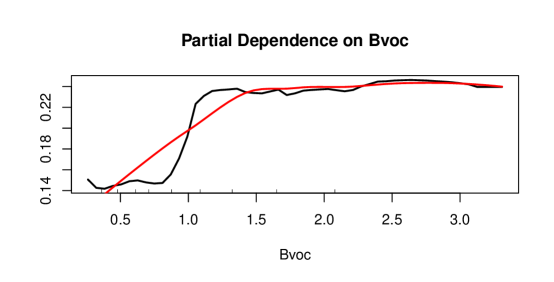
Figure 14: The fourth most important predictor of LRCs (Within-Cluster Spearman rank correlations between AACRmort and Bvoc) is Bvoc itself: $\%$IncMSE$=46.40$. This marginal relationship is also close to being monotone increasing. In fact, LRC’s of approximately $0.24$ correspond to all Bvoc levels above $1.20$.

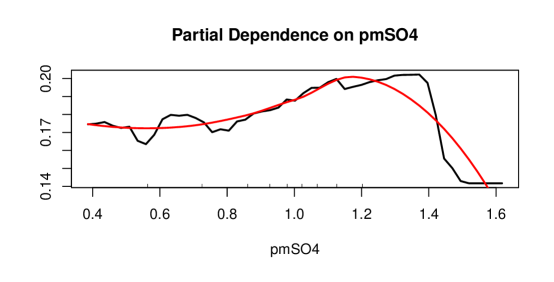
Figure 15: The predictor of LRCs in fifth place is $pmSO4:\%$IncMSE$=37.82$. This plot suggests a complex marginal relationship: LRCs steadily increase over the range $0.4\leq pmSO4\leq 1.4$, but then drop sharply when $pmSO4$ exceeds $1.4$.

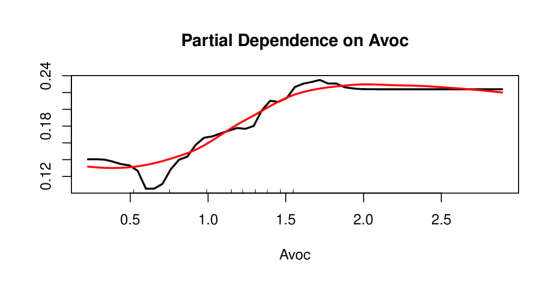
Figure 16: The sixth-place predictor of LRCs is Avoc: $\%$IncMSE$=25.26$. Here, LRC levels vaguely approximate a monotonically increasing marginal relationship, except for a rather large “dip” near Avoc$=0.6$ and a small decrease for Avoc $>1.7$. The general shape of this marginal relationship is somewhat like that of the Bvoc predictor in Figure 14.

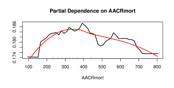
Figure 17: A seventh predictor of LRCs (between AACRmort and Bvoc) is AACRmort itself: $\%$IncMSE$=17.79$. Since the vertical range in this plot is quite small ($0.014$), any suggestion of “curvature” in this marginal relationship is probably unimportant.

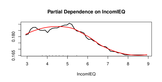
Figure 18: The last (and least important) predictor of within-cluster LRCs is IncomIEQ: $\%$IncMSE$=16.15$. This marginal relationship is complex but appears to monotonically decrease after a local mode near IncomIEQ$=5$.

Table 3 summarizes the key characteristics of our eight PDP plots. Note that the top 4 $X-$confounder variables predictive of AACRmort include the three variables inducing highest Incremental Node Purity.

TABLE 3 – Importance Statistics for $8$ Variables
Variable	%IncMSE	IncNodePurity
ASmoke	71.28070	16.611216
ChildPOV	59.45606	17.160771
PREMdeath	56.31122	11.765453
Bvoc	46.40073	16.198999
pmSO4	37.81722	12.071959
Avoc	25.25779	14.658269
AACRmort	17.79182	4.878167
IncomIEQ	16.14760	5.173446

5.3 Insights from a Single Recursive Partitioning Tree

We used the “model based” algorithms of Zeileis, Hothorn and Hornik (2008, 2015, 2022) to develop the relatively simple conditional regression-tree displayed in Figure 19. This tree has a maximal depth of $3$ and defines $7$ optimal “Bvoc intervals”. Within each interval, observed LRCs are predicted from local ASmoke levels using simple linear regression. Summary statistics for this tree are listed in Table $4$.

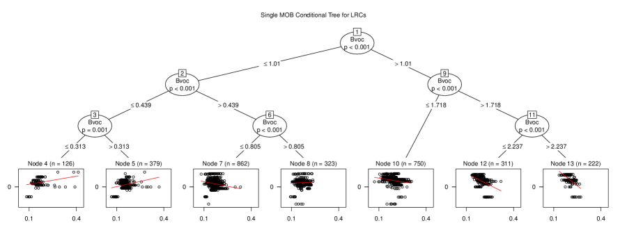
Figure 19: All 7 plots in the bottom row of this tree show $ASmoke$ rates that vary from less than 0.1 (i.e. $10\%$ of residents) to more than 0.4 ($40\%$) on their horizontal axis. On each vertical axis, estimated $LRC$s range from $-0.7$ to $+0.6$. Note that this RP Tree suggests that high ASmoke rates are particularly harmful within the two left-hand plots corresponding to low Bvoc $<0.44$ intervals. Within four of the five remaining higher Bvoc intervals on the the right-hand side of this MOB (model-based) tree, LRCs (between AACRmort and Bvoc) surprisingly appear to actually decrease as local ASmoke rates increase!

TABLE 4 – Statistics for LRC Prediction within 7 Bvoc Ranges
Final	Bvoc	Bvoc	LRC	ASmoke	US
Node	Range	Level	Intercept	Slope	Counties
4	0.261-0.313	Low	-0.00411	+1.09902	126
5	0.314-0.439	Low	-0.13183	+1.42106	379
7	0.440-0.805	Medium	0.33623	-1.24350	862
8	0.806-1.010	Medium	0.12447	+0.29020	323
10	1.011-1.718	High	0.45914	-1.01360	750
12	1.719-2.237	High	0.86823	-3.21152	311
13	2.238-3.309	High	1.31711	-5.09834	222

5.4 Advantages of Local Comparisons

Personal computers have helped shape statistical theory as well as its practice over the last 50 years. Freely available software can provide computational and visual fast-tracks into the strengths and weaknesses of alternative statistical methods. For example, the lower right-hand panel of Figure 10 showed just how misleading a scatter-plot can be that ignores cluster-membership. Our clusters contain US Counties with most similar $X-$characteristics, so they compare only “apples” with other “apples”, “potatoes” with other “potatoes”, etc.

Our LC strategy leads to fair local comparisons when the exposure variable is binary and to cogent local inferences when that exposure (say, Bvoc) is both continuous and correlated with potential confounding variables (such as Avoc, ASmoke, etc.)

A key feature of LC Strategy is that it creates a “new” variable of genuine interest for all observational units within each cluster. This variable contains either Local Treatment Differences (LTDs) when the exposure variable is Binary (New Treatment vs Standard Treatment) [Lopiano, Obenchain and Young (2014)] or else (Spearman) Local Rank Correlations (LRCs) when the exposure varies continuously. In this paper, our estimated LRCs quantify important new insights into potential relationships among environmental measures of genuine current interest.

6 Summary

Our eight PDP plots in Figures (11 through 18) and the summary statistics from Table 3 have encouraged us to focus our attention primarily on the top-four predictors of LRCs, where $Bvoc$ is number four. Again, neither $pmSOA\equiv Avoc+Bvoc$ nor either of its two components can apparently be actually “measured” today …using existing scientific instruments with reasonable accuracy.

Bvocs include terpenes from trees and grass, and EPA Bvoc predictions are, at least on average, positively correlated with corresponding local CDC CRmort counts, before and after being Age Adjusted. How will individual US environmentalists react to this “news”? Luckily, our single RP MOB tree in Figure 19 does suggest that levels of Bvoc $>1.01$ could be protective against high AACRmort rates when ASmoke rates are either average or higher!

Our final three Figures (20, 21 and 22) display US Maps that use shades of green, red or blue to color individual US Counties and, thereby, reveal interesting differences in patterns of variation in Bvoc, AACRmort or LRCs, respectively. These graphics illustrate just how varied and/or different these three quantities apparently are.

The future of NU Learning approaches for analysis of cross-sectional observational data strikes us as being quite promising. Unfortunately, traditional (Parametric and Supervised Learning) models used in Propensity Score estimation tend to be global (rather than local) and may make strong and potentially unrealistic assumptions.

Most interesting questions don’t have an answer that is clearly “Black” or “White”. Data from well-designed and well-executed experiments can illuminate some key issues. Meanwhile, large collections of observational data can reveal interesting real-world “shades of gray”.

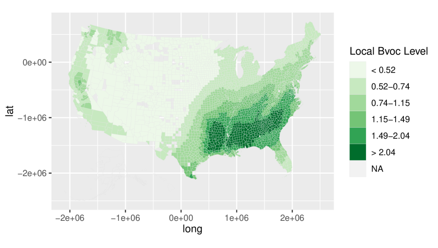
Figure 20: This US map [Kahle and Wickham (2013), Wickham (2016)] shows variation in EPA Bvoc predictions across US Counties using six shades of Green. Low Bvoc levels receiving the lightest shade of Green dominate the US “Great Plains” and Rocky Mountain regions where agricultural production is either low or supported by irrigation. Note that a vast majority of counties receive the same Bvoc color as their adjacent counties. Note also that 151 US Counties fall into the $7^{th}$ “NA” category and receive the see-through “background” color.

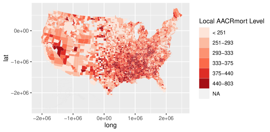
Figure 21: This map shows variation in AACRmort counts per $100,000$ residents using six shades of Red. These adjusted counts are certainly not smooth functions of geographic latitude and longitude; variation in AACRmort counts may result primarily from variation in the socioeconomic characteristics of local residents. After all, the vast majority of adjacent counties receive a somewhat different or very different shade of Red.

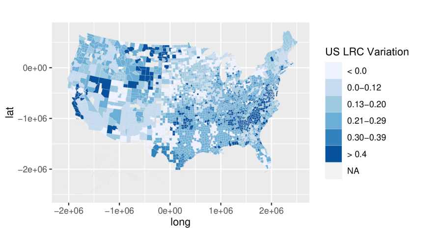
Figure 22: On this map showing variation in Local Rank Correlations (LRCs) across US Counties, six shades of Blue identify LRC levels of association between AACRmort and Bvoc within our 50 clusters of US counties well-matched in the $7-$dimensional space of potential confounded characteristics. Note that all adjacent counties receiving different shades of Blue must be in different Clusters and thus have somewhat different characteristics. All $421$ counties with negative LRC estimates receive the lightest shade of Blue. Again, 151 counties without data receive the see-through “background” color.

Our use of LC Strategy in our analysis of rather voluminous and detailed data highlights a truly key advantage of our computer intensive approach. Namely, this approach generates many highly informative graphical displays that range from rather simplistic to quite detailed. Examining a wide variety of graphics can guide further analyses in unanticipated directions. For example, note the great detail embedded within Figures 19, 20, 21 and 22. Such plots enable comparisons among US counties that are “similar” in terms of either Cluster Membership in three dimensions (AACRmort, Bvoc and ASmoke) or Geography in two dimensions (latitude and longitude).

6.1 Contributions to Data and Code Sharing

Our reconstruction of the data used in Pye et al. (2021) can be found in the pmdata data.frame that is part of the newest Version ($1.4$) of the LocalControlStrategy R-package, Obenchain (2015-2022). Alternatively, a CSV file containing only $25$ key variables can be downloaded from dryad, Young and Obenchain (2022), https://doi.org/10.5061/dryad.63xsj3v58. These data are as much “like” the CDC and EPA data used by Pye et al. (2021) as is possible by private US citizens.

Internet site http://localcontrolstatistics.org contains an archive, LCS$\_$EPA$\_$archive.zip, that can be freely downloaded. This archive contains $R-$code that performs the basic analyses and displays examples of figures from this paper. A wide variety of introductory information about using LC Strategy for statistical NU Learning can also be read at or downloaded from this site.

6.2 Insights from a New Statistical Perspective

Our use of LC Strategy has lead to findings that are fundamentally different from and quite possibly more relevant and technically sound than those of Pye et al. (2021). Since interaction effects abound within the data, it’s certainly not surprising that our LRC distribution (Figure 8) from simple local (within cluster) models and our $RP-$Tree model of Figure 19 each provide insights more clear and informative than complex EPA models. While EPA models can be claimed to be “smooth and continuous”, they are embedded within an abstract high-dimensional $X-$space of confounded variables.

6.3 Our Focus on Biogenic Volatile Organic Compounds

It became clear in our earliest data analyses that $Bvoc$ would be a better predictor of $AACRmort$ than either $Avoc$ or $pmSOA\equiv Avoc+Bvoc$. In fact, as shown in Table 5, the Spearman Rank Correlations between $Bvoc$ and all six other key measures are higher than those of $Avoc$. Only the single Pearson correlation of $Avoc$ with Sulfates ($pmSO4$) is larger than its corresponding correlation with $Bvoc$. Furthermore, all $\beta-$coefficient estimates of $Avoc$ effects on $AACRmort$ are negative or zero in Figure 2.

TABLE 5 – Pearson and Spearman Correlations between Variables
Method		AACRmort	PREMdeath	pmSO4	ASmoke	ChildPOV	IncomIEQ
——-	—-	——	——	——	——	——	——
Pearson	Bvoc	0.4589	0.4217	0.5023	0.4622	0.4884	0.4163
Pearson	Avoc	0.2489	0.0890	0.7228	0.3271	0.1134	0.1393
——-	—-	——	——	——	——	——	——
Spearman	Bvoc	0.4740	0.4808	0.6195	0.5437	0.4950	0.4154
Spearman	Avoc	0.2458	0.1475	0.6137	0.3763	0.1145	0.1467

6.4 Revealing Effect Heterogeneity

As is clear from Figure 8, our distribution of LRC estimates resulting from using $K=50$ “Ward.D” Clusters displays considerable heterogeneity. Furthermore, $40$ of our $50$ Clusters yield positive LRC estimates between $AACRmort$ and $Bvoc$ and contain almost $86\%$ of the $2,973$ US Counties without missing data. Table $6$ displays some added detail on the $16$ Clusters with “highly significant” (one-tailed) probabilities. Only the $3$ Clusters listed at the bottom of Table $6$ have negative LRC estimates and contain a total of $86$ US Counties; these are the only $86$ US locations where AACRmort levels tend to monotonically decrease as Bvoc levels increase. The genuinely “bad news” here is that $6$ of the $13$ Clusters at the top of Table $6$ have positive LRCs that are even more highly significant than the most significant negative LRCs! Unfortunately, within these $916$ US Counties, AACRmort levels tend to monotonically increase as Bvoc levels increase! Finally, we note that $Bvoc=terpenes+isoprenes$, where terpenes clearly appear to be the more “active” sub-component of Bvoc. Data on pmTOT ($PM_{2.5}$) and $27$ of its sub-components are contained in our pmdata R data.frame.

TABLE 6 – 16 Clusters with Highly Significant (Spearman) LRCs
Cluster	Number of	Spearman	One-Tailed	Sig-Level
Number	US Counties	LRC	Probability	Symbol
1	83	+0.277	0.006	$**$
2	52	+0.393	0.002	$**$
6	58	+0.478	0.0001	$****$
8	63	+0.303	0.008	$**$
10	56	+0.391	0.002	$**$
11	61	+0.511	0.00002	$****$
14	115	+0.267	0.002	$**$
17	34	+0.518	0.001	$***$
32	127	+0.292	0.0005	$***$
39	72	+0.376	0.0006	$***$
40	56	+0.537	0.00002	$****$
41	99	+0.295	0.002	$**$
46	40	+0.405	0.005	$**$
–	–	——	——	—–
4	35	-0.414	0.007	$**$
26	39	-0.404	0.006	$**$
49	12	-0.699	0.007	$**$

6.5 Our Bottom Line

There appear to be only two realistic conclusions from the EPA data that we analyze here. Either biogenic volatile organic compounds are real killers, or current EPA models for the chemical content of air pollution are misleadingly wrong.

Conflict of Interest

As independent and self-funded researchers, the authors declare that no competing interests exist.

References

- [1] Breiman, L. (2001), “Random Forests”, Machine Learning, 45, 532. https://doi.org/10.1023/A:1010933404324.
- [2] Breiman, L. (2002), “Manual On Setting Up, Using, And Understanding Random Forests, V3.1”. https://www.stat.berkeley.edu/~breiman/Using_random_forests_V3.1.pdf.
- [3] Centers for Disease Control and Prevention National Center for Health Statistics. Compressed Mortality File 1999-2016 on CDC WONDER Online Database, released June 2017. Data are from the Compressed Mortality File 1999-2016 Series 20 No.2U, 2016, as compiled from data provided by the 7 vital statistics jurisdictions through the Vital Statistics Cooperative Program. Accessed by Obenchain on 19 April 2022, http://wonder.cdc.gov/cmf-icd10.html.
- [4] Friedman, J. (2001), “Greedy function approximation: the gradient boosting machine”, Annals of Statistics, 29(5), 11891232, https://doi.org/10.1214/aos/1013203451.
- [5] Glaeser, E.L. (2006), “Researcher incentives and empirical methods”, https://www.nber.org/system/files/working_papers/t0329/t0329.pdf.
- [6] Hothorn, T. and Zeileis, A. (2015), “partykit: A Modular Toolkit for Recursive Partytioning in R.”, Journal of Machine Learning Research, 16, 39053909. https://jmlr.org/papers/v16/hothorn15a.html.
- [7] Hothorn, T., Seibold, H. and Zeileis, A. (2015-2022), “partykit: A Modular Toolkit for Recursive Partytioning”, ver 1.2-16, https://CRAN.R-project.org/package=partykit.
- [8] Kahle, D. and Wickham, H. (2013), “ggmap: Spatial Visualization with ggplot2.”, The R Journal, 5, 144161. http://journal.r-project.org/archive/2013-1/kahle-wickham.pdf.
- [9] Koenker, R. (2005 - 2022), “quantreg: Quantile Regression”, ver 5.94, https://CRAN.R-project.org/package=quantreg.
- [10] Liaw, A. and Wiener, M. (2002 - 2022) “randomForest: Breiman and Cutler’s Random Forests for Classification and Regression”, ver 4.7-1, https://CRAN.R-project.org/package=randomForest.
- [11] Logan, W.P.D. (1953), “Mortality in the London Fog Insident”, Lancet, 261, 336338, https://doi.org/10.1016/S0140-6736(53)91012-5.
- [12] Lopiano, K.K., Obenchain, R.L. and Young, S.S. (2014), “Fair Treatment Comparisons in Observational Research”, Statistical Analysis and Data Mining, 7, 376384. https://doi.org/10.1002/sam.11235.
- [13] Obenchain, R.L. (1971), “Multivariate Procedures Invariant under Linear Transformations, Annals of Mathematical Statistics, 42: 15691578. https://doi.org/10.1214/aoms/1177693155.
- [14] Obenchain, R.L. (2005-2022), “RXshrink: Maximum Likelihood Shrinkage using Generalized Ridge or Least Angle Regression Methods”, ver 2.1, https://CRAN.R-project.org/package=RXshrink.
- [15] Obenchain, R.L. (2015-2022), “LocalControlStrategy: Local Control Strategy for Robust Analysis of Cross-Sectional Data”, ver 1.4, https://CRAN.R-project.org/package=LocalControlStrategy.
- [16] Obenchain, R.L. (2022), “Efficient Generalized Ridge Regression, Open Statistics, 3: 118. https://doi.org/10.1515/stat-2022-0108.
- [17] Obenchain, R.L. and Young, S.S. (2013), “Advancing statistical thinking in health care research”, Journal of Statistical Theory and Practice, 7, 456469. https://doi.org/10.1080/15598608.2013.772821.
- [18] Obenchain, R.L., Young, S.S. and Krstic, G. (2019), “Low-level Radon Exposure and Lung Cancer Mortality”, Regulatory Toxicology and Pharmacology, 107, https://doi.org/10.1016/j.yrtph.2019.104418.
- [19] Pye, H.O.T., Ward-Caviness, C.K., Murphy, B.N., Appel, K.W. and Seltzer, K.M. (2021), “Secondary organic aerosol association with cardiorespiratory disease mortality in the United States”. Nature Communications 12, 7215. https://doi.org/10.1038/s41467-021-27484-1.
- [20] R Core Team. (2022), “R: A language and environment for statistical computing”. https://www.R-project.org/
- [21] Rubin, D.B. (1980), “Bias reduction using Mahalanobis metric matching”. Biometrics, 36, 293298. https://www.jstor.org/stable/2529981.
- [22] Rubin, D.B. (2008), “For objective causal inference, design trumps analysis”, Annals of Applied Statistics, 2, 808840. https://doi:10.1214/08-AOAS187.
- [23] Stang, P.E., Ryan, P.B., Racoosin, J.A., Overhage, J.M., Hartzema, A.G., Reich, C., Welebob, E., Scarnecchia, T. and Woodcock, J. (2010), “Advancing the Science for Active Surveillance: Rationale and Design for the Observational Medical Outcomes Partnership”. Annals of Internal Medicine, 153, 600606. https://doi.org/10.7326/0003-4819-153-9-201011020-00010.
- [24] Stuart, E.A. (2010), “Matching methods for causal inference: A review and a look forward”. Statistical Science, 25, 121. https://doi:10.1214/09-STS313.
- [25] U.S. EPA Office of Research and Development. (2019), “CMAQ (Version 5.3.1)”, https://doi.org/10.5281/zenodo.3585898.
- [26] Volkamer, R., Jimenez, J.L., San Martini, F., Dzepina, K., Qi, Z., Salcedo, D., Molina, L.T., Worsnop, D.R. and Molina, M.J. (2006), “Secondary organic aerosol formation from anthropogenic air pollution: Rapid and higher than expected”. Geophys. Res. Lett. https://doi.org/10.1029/2006GL026899.
- [27] Welch, W.J. (1990), “Construction of permutation tests.” Journal American Statistical Association, 85, 693698. https://doi.org/10.1080/01621459.1990.10474929.
- [28] Wickham, H. (2016), “ggplot2: Elegant Graphics for Data Analysis”. New York: Springer-Verlag.
- [29] Wood, S. N. (2003), “Thin plate regression splines”. J. R. Stat. Soc. B. Met. 65, 95114. https://doi.org/10.1111/1467-9868.00374.
- [30] Wood, S. N. (2004), “Stable and efficient multiple smoothing parameter estimation for generalized additive models”. Journal American Statistical Association, 99, 673686. https://doi.org/10.1198/016214504000000980.
- [31] Wood, S. N. (2022), “mgcv: Mixed GAM Computation Vehicle with Automatic Smoothness Estimation”, https://CRAN.R-project.org/package=mgcv.
- [32] van der Laan, M. and Rose, S. (2010), “Statistics ready for a revolution: Next generation of statisticians must build tools for massive data sets”. AMStat News, September, 38–39. https://magazine.amstat.org/blog/2010/09/01/statrevolution/.
- [33] Volkamer, R., Jimenez, J., San Martini, F., Dzepina, K., Qi, Z., Salcedo, D., Molina, L., Worsnop, D., and Molina, M. (2006). “Secondary organic aerosol formation from anthropogenic air pollution: Rapid and higher than expected. Geophys. Res. Lett. https://doi.org/10.1029/2006GL026899.
- [34] Young, S.S., Kindzierski, W. and Randall, D. (May 2021), “Shifting Sands: Unsound Science and Unsafe Regulation. Report : Keeping Count of Government Science – P-Value Plotting, P-Hacking, and PM2.5 Regulation”. National Association of Scholars. https://files.eric.ed.gov/fulltext/ED616199.pdf.
- [35] Young, S.S., Obenchain, R.L. (August 2022), “EPA Particulate Matter Data”. https://doi.org/10.5061/dryad.63xsj3v58.
- [36] Young, S.S., Smith, R.L. and Lopiano, K.K. (2017), “Air Quality and Acute Deaths in California, 20002012”, Regulatory Toxicology and Pharmacology, 88, 173184. https://doi.org/10.1016/j.yrtph.2017.06.003.
- [37] Zeileis, A., Hothorn, T. and Hornik, K. (2008). “Model-Based Recursive Partitioning.” Journal of Computational and Graphical Statistics, 17, 492514. https://doi.org/10.1198/106186008X319331.