A hybridizable discontinuous Galerkin method on unfitted meshes for single-phase Darcy flow in fractured porous media

Abstract.

We present a novel hybridizable discontinuous Galerkin (HDG) method on unfitted meshes for single-phase Darcy flow in a fractured porous media. In particular we apply the HDG methodology to the recently introduced reinterpreted discrete fracture model (RDFM) [1] that use Dirac-$\delta$ functions to model both conductive and blocking fractures. Due to the use of Dirac-$\delta$ function approach for the fractures, our numerical scheme naturally allows for unfitted meshes with respect to the fractures, which is the major novelty of the proposed scheme. Moreover, the scheme is locally mass conservative and is relatively easy to implement comparing with existing work on the subject. In particular, our scheme is a simple modification of an existing regular Darcy flow HDG solver by adding the following two components: (i) locate the co-dimension one fractures in the background mesh and adding the appropriate surface integrals associated with these fractures into the stiffness matrix, (ii) adjust the penalty parameters on cells cut through conductive and blocking fractures (fractured cells).

Despite the simplicity of the proposed scheme, it performs extremely well for various benchmark test cases in both two- and three-dimensions. This is the first time that a truly unfitted finite element scheme been applied to complex fractured porous media flow problems in 3D with both blocking and conductive fractures without any restrictions on the meshes.

1. Introduction

Many applications in contaminant transportation, petroleum engineering and radioactive waste deposit can be modeled by single- and multi-phase flows in porous media. A typical porous media may contain conductive fractures with tiny thickness but high permeability. Some fractures may be filled with minerals and debris, forming blocking fractures with low permeability. Mathematical modeling and numerical simulation for flows in fractured porous media are challenging due to the highly heterogeneity of the porous media.

Several effective mathematical models have been developed in the literature for simulating flows in porous media with conductive fractures, such as the dual porosity model [2, 3, 4], single porosity model [5], traditional discrete fracture model (DFM) [6, 7, 8, 9, 10, 11, 12], embedded DFM (EDFM) [13, 14, 15, 16, 17, 18, 19], the interface models [20, 21, 22, 23] and extended finite element DFM (XDFM) based on the interface models [24, 25, 26, 27, 28], finite element method based on Lagrange multipliers [29, 30, 31], etc. Among the above mentioned works, the interface model [32, 33, 34, 35] and the projection-based EDFM (pEDFM) [16, 36] can also be used for problems containing blocking fractures. The interface model is to explicitly represent the fracture as the interface of a porous media, and the governing equations in the porous media and fractures can be constructed. In the interface model, the matrix and fractures are considered as two different system and the mass transfer between them is given by the jump of the velocity. Therefore, the interface model requires fitted mesh, i.e. the fracture is located at the cell skeletons. Though hanging nodes are allowed, numerical methods based on fitted meshes may suffer from low quality meshes. To fix this gap, XDFM [24, 25, 26, 27, 28] was introduced. However, such treatment may significantly increase the degrees of freedom (DoFs), hence is not of practical use, especially for problems with high geometrical complexity [37]. Another possibility to extend the interface model to unfitted mesh is to use the CutFEM [38]. However, this method may not work for media with complicated fractures, as the fractures have to separate the domain into completely disjoint subdomains. The pEDFM [16, 36] is another way to simulate flow in porous media with blocking fractures. The basic idea is to reduce the effective flow area between the blocking fracture and the adjacent matrix cells based on the property of the blocking fracture. However, most of previous works in this direction work for rectangular meshes, and the extension to general triangular or arbitrary meshes seems to be complicated.

In [39], one of the authors introduced the reinterpreted discrete fracture model (RDFM) for single-phase flow in porous media with conductive fractures. Different from the interface model and pEDFM, the RDFM couples the fracture and matrix in one system and use one equation to model the flows in both matrix and fractures. The basic idea is to use Dirac-$\delta$ functions to represent the lower dimensional fractures in the system containing higher dimensional matrix. The effect of the Dirac-$\delta$ functions is to increase the permeability at the location of the conductive fractures. Later, the RDFM was successfully applied to simulate contaminant transportation in [40]. As an extension, the RDFM was further developed to simulate flows in porous media with both conductive and blocking fractures in [1]. Similar to the RDFM for conductive fractures [39], the blocking fractures were also described as Dirac-$\delta$ functions, and they are used to increase the flow resistance. The RDFM incorporates the information of the fractures into the equation, hence it works for arbitrary meshes without any restrictions. In [1], the local discontinuous Galerkin (LDG) methods were applied to RDFM. An extremely large penalty of order $\mathcal{O}(h^{-3})$ was added to the pressure on cell interfaces without blocking fractures, while a moderate large penalty of order $\mathcal{O}(h^{-2})$ was applied to the normal direction of the velocity on cell interfaces with blocking fractures. The penalty is used to intimate the continuity requirement of the target variables. Unfortunately, this LDG method leads to a fully coupled saddle-point linear system for the velocity and pressure, hence its practical application in three dimension is limited. Moreover, the lowest order scheme therein use (discontinuous) piecewise linear functions as the piecewise constant version did not lead to a convergent algorithm. Furthermore, the effect of the penalty and well-posedness of the method was not clear. Besides the above works, the RDFM for blocking fractures was also combined with the interface model for conductive fractures in [41] where fitted meshes for conductive fractures were required.

In this paper, we apply the hybridizable discontinuous Galerkin (HDG) methods for RDFM-based single-phase flows in porous media. Similar to the idea given in [1], the proposed method (1) produces locally conservative velocity approximations; (2) works for problems containing both conductive and blocking fractures; (3) can be applied to arbitrary meshes without any restrictions. In additional to the above, there are several advantages of the proposed method that were not enjoyed by the one given in [1]. First of all, the HDG method can be efficiently solved via static condensation, which leads to a symmetric positive definite (SPD) linear system for the pressure degrees of freedom (DOFs) on the mesh skeletons only. Hence they can be implemented very efficiently comparing with the LDG scheme [1]. As a result, three-dimensional simulation for complex fracture networks are now possible. Secondly, the penalty parameters in the HDG scheme is only adjusted on cells contain fractures, with extra (pressure) stabilization on conductive fractures and reduced (pressure) stabilization on blocking fractures. With a judicious choice of the penalty parameters, the lowest order HDG scheme with piecewise constant approximations can now yield satisfactory numerical results. Finally, the well-posedness of the proposed method can be guaranteed theoretically, which was completely missing for the method given in [1]. As an application, it is straightforward to couple the proposed flow equation with the transport equations and construct the locally conservative numerical methods for the transport equations. However, that is not the main target of this paper, so we will discuss the applications in the future. The combination of these properties for the HDG scheme on unfitted meshes makes it highly competitive comparing with existing works for fractured porous media that can simultaneously handle blocking and conductive fractures both in terms of algorithmic complexity and numerical accuracy.

The rest of the paper is organized as follows. In Section 2, we present the RDFM and the HDG methods to be used. Numerical results for various benchmark test cases are presented in Section 3. Some concluding remarks will be given in Section 4.

2. The HDG scheme

2.1. The model

We consider the following RDFM proposed in [1]:

$$\left(\hbox{\boldmath$I$}+\hbox{\boldmath$K$}_{m}\sum_{i=1}^{M}\frac{\epsilon_{i}}{k_{i}}\delta_{\Gamma_{i}}\hbox{\boldmath$n$}_{i}\hbox{\boldmath$n$}_{i}^{T}\right)\hbox{\boldmath$u$}= \;-\left(\hbox{\boldmath$K$}_{m}+\sum_{i=M+1}^{M+N}{\epsilon_{i}}{k_{i}}\delta_{\Gamma_{i}}(\hbox{\boldmath$I$}-\hbox{\boldmath$n$}_{i}\hbox{\boldmath$n$}_{i}^{T})\right)\nabla p,$$ (1a)

$$\nabla\cdot\hbox{\boldmath$u$}= \;f,$$ (1b)

on a $$d \Omega d=2,3 u p \hbox{\boldmath$K$}_{m} I f \Gamma_{i} i (d-1) \epsilon_{i} k_{i} \hbox{\boldmath$n$}_{i} 1\leq i\leq M+N M N k_{i}\ll\hbox{\boldmath$K$}_{m} i\leq M k_{i}\gg\hbox{\boldmath$K$}_{m} i\geq M+1$$-dimensional domain with . Here is the total Darcy velocity, the pressure, is the matrix permeability, is the identity tensor, is the source term, and is the location of the -th -dimensional fracture with thickness , permeability and normal direction for , where we assume the first fractures are blocking while the last fractures are conductive, i.e., for and for .

Moreover, $\delta_{\Gamma_{i}}$ is the Dirac-$\delta$ function such that $\delta_{\Gamma_{i}}(\hbox{\boldmath$x$})=\infty$ if $\hbox{\boldmath$x$}\in\Gamma_{i}$, $\delta_{\Gamma_{i}}(\hbox{\boldmath$x$})=0$ if $\hbox{\boldmath$x$}\not\in\Gamma_{i}$ and $\int_{\Omega}\delta_{\Gamma_{i}}\mathrm{dx}=1$. For simplicity, we assume the model (1) is equiped with the homogeneous Dirichlet boundary condition $p=0$ on $\partial\Omega$. Other boundary conditions will be used in the numerical experiments.

Remark 2.1 (On RDFM).

In (1), we apply Dirac-$\delta$ functions to bridge the difference of the dimensions between the matrix and fractures as the Dirac-$\delta$ functions concentrate all the information at its concentration. The first $M$ Dirac-$\delta$ functions are used to increase the flow resistance and are for blocking fractures. Due to the small thickness of the blocking fractures, the effect of the blocking fractures in the tangential direction is negligible. Therefore, we include the tensor associate with the normal direction in the model. Similarly, the last $N$ Dirac-$\delta$ functions are used to increase the permeability and are for conductive fractures. Moreover, due to the small thickness of the blocking fractures, the effect of the conductive fractures in the normal direction is negligible, and we include the tensor associate with the tangential directions in the model. We refer to [39] and [1] for more discussion on the RDFM.

The Dirac-$\delta$ function approach in the above model avoids a direct modeling of the fractures using lower dimensional Darcy flows as typical in the interface models [32, 33, 34, 35]. Hence, unfitted mesh discretizations can be naturally applied. In the original work [1], an LDG scheme on unfitted meshes was devised for (1) in two dimensions with satisfactory numerical results. However, well-posedness of the LDG scheme was not established as no energy identity exists, and its computational cost is relatively large comparing with existing works on (partially) fitted meshes.

Here we will devise a well-posed HDG scheme on unfitted meshes for the above model (1), which is not only computationally cheaper than the LDG scheme [1] but also more accurate and has an energy identity. To this end, we introduce the Darcy velocity in the matrix $\widetilde{\hbox{\boldmath$u$}}:=-\hbox{\boldmath$K$}_{m}\nabla p$ as a new unknown and rewrite the model (1) into the following three-field formulation:

$$\left(\hbox{\boldmath$K$}_{m}^{-1}+\sum_{i=1}^{M}\frac{\epsilon_{i}}{k_{i}}\delta_{\Gamma_{i}}\hbox{\boldmath$n$}_{i}\hbox{\boldmath$n$}_{i}^{T}\right)\hbox{\boldmath$u$}= \;\left(\hbox{\boldmath$I$}+\sum_{i=M+1}^{M+N}\hbox{\boldmath$K$}_{m}^{-1}{\epsilon_{i}}k_{i}\delta_{\Gamma_{i}}(\hbox{\boldmath$I$}-\hbox{\boldmath$n$}_{i}\hbox{\boldmath$n$}_{i}^{T})\right)\hbox{\boldmath$K$}_{m}^{-1}\widetilde{\hbox{\boldmath$u$}},$$ (2a)

$$\hbox{\boldmath$K$}_{m}^{-1}\widetilde{\hbox{\boldmath$u$}}+\nabla p= \;0,$$ (2b)

$$\nabla\cdot\hbox{\boldmath$u$}= \;f,$$ (2c)

Note that we multiplied equation (1a) with $\hbox{\boldmath$K$}_{m}^{-1}$ on the left to obtain the equation (2a). We emphasis that here $u$ is the total Darcy velocity that contains information about the fractures, whilst $\widetilde{\hbox{\boldmath$u$}}$ is the Darcy velocity on the matrix without fracture contributions.

2.2. The HDG scheme

Let $\mathcal{T}_{h}:=\{K\}$ be a triangulation of the domain $\Omega$ that is unfitted to the location of the fractures. Let $\mathcal{E}_{h}$ be the collections of $(d-1)$-dimensional facets (edges for $d=2$, faces for $d=3$) of $\mathcal{T}_{h}$. We use level set functions to represent the fractures $\Gamma_{i}$. In particular,

• if $\Gamma_{i}$ is a closed curve/surface without boundaries, it is simply approximated by the zero level set of a continuous piecewise linear function $\phi_{i}\in W_{h}^{1}\cap H^{1}(\Omega)$ on the mesh $\mathcal{T}_{h}$:

  $$\Gamma_{i,h}:=\{x\in\Omega:\phi_{i}(x)=0\}.$$

• if $\Gamma_{i}$ is a closed curve/surface with $(d-2)$-dimensional boundary $\partial\Gamma_{i}$, it is approximated by a main level set function $\phi_{i}\in W_{h}^{1}\cap H^{1}(\Omega)$ for the (extended) surface $\Gamma_{i}$ and additional level set functions $\psi_{i}^{j}\in W_{h}^{1}\cap H^{1}(\Omega)$ for $j=1,\cdots L$ to take care of the boundary $\partial\Gamma_{i}$:

  $$\Gamma_{i,h}:=\{x\in\Omega:\phi_{i}(x)=0\}\cap_{j=1}^{L}\{x\in\Omega:\psi_{i}^{j}(x)<0\}.$$

  In practice, usually two level set functions are sufficient to provide a good approximation of $\Gamma_{i}$, i.e.,

  $$\Gamma_{i,h}:=\{x\in\Omega:\phi_{i}(x)=0\}\cap\{x\in\Omega:\psi_{i}^{1}(x)<0\}.$$

Hence the discrete fractures $\Gamma_{i,h}$ on each element $K\in\mathcal{T}_{h}$ is always a line segment in 2D or a polygon in 3D due to the use of piecewise linear functions as level sets. With $\Gamma_{i,h}$ ready, we split the cells in $\mathcal{T}_{h}$ into disjoint three groups

$$\mathcal{T}_{h}:=\mathcal{T}_{h}^{r}\cup\mathcal{T}_{h}^{b}\cup\mathcal{T}_{h}^{c},$$

where $\mathcal{T}_{h}^{r}$ contains regular cells without fractures, $\mathcal{T}_{h}^{b}$ contains cells with blocking fractures, and $\mathcal{T}_{h}^{c}$ contains cells with conductive fractures defined as follows:

$$\mathcal{T}_{h}^{b}:= \;\{K\in\mathcal{T}_{h}: \;\exists i\in[1,M]\text{ such that }K\cap\Gamma_{i,h}\not=\emptyset\},$$

$$\mathcal{T}_{h}^{c}:= \;\{K\in\mathcal{T}_{h}\backslash\mathcal{T}_{h}^{b}: \;\exists i\in[M+1,M+N]\text{ such that }K\cap\Gamma_{i,h}\not=\emptyset\},$$

$$\mathcal{T}_{h}^{r}:= \;\mathcal{T}_{h}\backslash\{\mathcal{T}_{h}^{b}\cup\mathcal{T}_{h}^{c}\}.$$

Note that when both blocking and conductive fractures appear in a cell, we always treat it as a blocking cell in $\mathcal{T}_{h}^{b}$ and we will ignore the conductive fractures within that cell in the discretization for stability considerations. Note also that we allow fractures to be intersecting with each other in an arbitrary fashion within a single cell as long as a discrete characterization of the fracture $\Gamma_{i,h}$ using (multi-)level sets is possible.

Given a polynomial degree $k\geq 0$, we consider the following finite element spaces:

$$\hbox{\boldmath$V$}_{h}^{k}:= \;\{\hbox{\boldmath$v$}\in[L^{2}(\mathcal{T}_{h})]^{d}:\;\hbox{\boldmath$v$}|_{K}\in[P_{k}(K)]^{d},\quad\forall K\in\mathcal{T}_{h}\},$$ (3a)

$$W_{h}^{k}:= \;\{w\in L^{2}(\mathcal{T}_{h}):\;w|_{K}\in P_{k}(K),\quad\forall K\in\mathcal{T}_{h}\},$$ (3b)

$$M_{h}^{k}:= \;\{\mu\in L^{2}(\mathcal{E}_{h}):\;\mu|_{F}\in P_{k}(F),\quad\forall F\in\mathcal{E}_{h},\quad\mu|_{F}=0\text{ on }\partial\Omega\},$$ (3c)

where $P_{k}(S)$ is the polynomial space of degree $k$ on $S$. We further denote the following inner products to simplify notation:

$$(\phi,\psi)_{\mathcal{T}_{h}}:= \;\sum_{K\in\mathcal{T}_{h}}\int_{K}\phi\,\psi\,\mathrm{dx}, \quad\quad\langle\phi,\psi\rangle_{\partial\mathcal{T}_{h}}:=\;\sum_{K\in\mathcal{T}_{h}}\int_{\partial K}\phi\,\psi\,\mathrm{ds}.$$

The HDG scheme for (2) is now given as follows: Find $(\hbox{\boldmath$u$}_{h},\widetilde{\hbox{\boldmath$u$}}_{h},p_{h},\widehat{p}_{h})\in\hbox{\boldmath$V$}_{h}^{k}\times\hbox{\boldmath$V$}_{h}^{k}\times W_{h}^{k}\times M_{h}^{k}$ such that

$$(\hbox{\boldmath$K$}_{m}^{-1}\hbox{\boldmath$u$}_{h},\widetilde{\hbox{\boldmath$v$}}_{h})_{\mathcal{T}_{h}}+\Phi_{b}(\hbox{\boldmath$u$}_{h},\widetilde{\hbox{\boldmath$v$}}_{h})=\;(\hbox{\boldmath$K$}_{m}^{-1}\widetilde{\hbox{\boldmath$u$}}_{h},\widetilde{\hbox{\boldmath$v$}}_{h})_{\mathcal{T}_{h}}+\Phi_{c}(\widetilde{\hbox{\boldmath$u$}}_{h},\widetilde{\hbox{\boldmath$v$}}_{h}),$$ (4a)

$$(\hbox{\boldmath$K$}_{m}^{-1}\widetilde{\hbox{\boldmath$u$}}_{h},\hbox{\boldmath$v$}_{h})_{\mathcal{T}_{h}}-(p_{h},\nabla\cdot\hbox{\boldmath$v$}_{h})_{\mathcal{T}_{h}}+\langle\widehat{p}_{h},\hbox{\boldmath$v$}_{h}\cdot\hbox{\boldmath$n$}\rangle_{\partial\mathcal{T}_{h}}= \;0,$$ (4b)

$$-(\hbox{\boldmath$u$}_{h},\nabla q_{h})_{\mathcal{T}_{h}}+\langle\widehat{\hbox{\boldmath$u$}}_{h}\cdot\hbox{\boldmath$n$},q_{h}\rangle_{\partial\mathcal{T}_{h}}= \;(f,q_{h})_{\mathcal{T}_{h}},$$ (4c)

$$\langle\widehat{\hbox{\boldmath$u$}}_{h}\cdot\hbox{\boldmath$n$},\widehat{q}_{h}\rangle_{\partial\mathcal{T}_{h}}= \;0,$$ (4d)

for all $$(\hbox{\boldmath$v$}_{h},\widetilde{\hbox{\boldmath$v$}}_{h},q_{h},\widehat{q}_{h})\in\hbox{\boldmath$V$}_{h}^{k}\times\hbox{\boldmath$V$}_{h}^{k}\times W_{h}^{k}\times M_{h}^{k} \Phi_{b} \Phi_{c} \delta$$, where / contain the following blocking/conductive fracture surface integrals (taking into account the property of the Dirac- functions):

$$\Phi_{b}(\hbox{\boldmath$u$},\hbox{\boldmath$v$}):= \;\sum_{K\in\mathcal{T}_{h}^{b}}\sum_{i=1}^{M}\int_{K\cap\Gamma_{i,h}}\frac{\epsilon_{i}}{k_{i}}(\hbox{\boldmath$u$}\cdot\hbox{\boldmath$n$}_{i})(\hbox{\boldmath$v$}\cdot\hbox{\boldmath$n$}_{i})\,\mathrm{ds},$$ (4e)

$$\Phi_{c}(\hbox{\boldmath$u$},\hbox{\boldmath$v$}):= \;\sum_{K\in\mathcal{T}_{h}^{c}}\sum_{i=M+1}^{M+N}\int_{K\cap\Gamma_{i,h}}\epsilon_{i}k_{i}(\hbox{\boldmath$K$}_{m}^{-1}\hbox{\boldmath$u$})_{t,i}\cdot(\hbox{\boldmath$K$}_{m}^{-1}\hbox{\boldmath$v$})_{t,i}\,\mathrm{ds},$$ (4f)

where $$(\hbox{\boldmath$w$})_{t,i}:=\hbox{\boldmath$w$}-(\hbox{\boldmath$w$}\cdot\hbox{\boldmath$n$}_{i})\hbox{\boldmath$n$}_{i} w \Gamma_{i,h} \widehat{\hbox{\boldmath$u$}}_{h}\cdot\hbox{\boldmath$n$}$$ denotes the tangential component of a vector on , and the numerical flux takes the following form:

$$\widehat{\hbox{\boldmath$u$}}_{h}\cdot\hbox{\boldmath$n$}:=\hbox{\boldmath$u$}_{h}\cdot\hbox{\boldmath$n$}+\alpha_{h}(p_{h}-\widehat{p}_{h}),$$ (4g)

with $$\alpha_{h}>0$$ being the stabilization function defined element-wise as follows:

$$\alpha_{h}|_{K}=\left\{\begin{tabular}[]{ll}$\hbox{\boldmath$K$}_{m}$&if $K\in\mathcal{T}_{h}^{r}$,\\[2.15277pt] $C_{b}(h_{K}/L)^{s_{b}}\hbox{\boldmath$K$}_{m}$&if $K\in\mathcal{T}_{h}^{r}$,\\[2.15277pt] $C_{c}\,(h_{K}/L)^{-s_{c}}\hbox{\boldmath$K$}_{m}$&if $K\in\mathcal{T}_{h}^{c}$,\end{tabular}\right.$$ (4k)

where $$h_{K} L \Omega C_{b},C_{c}>0 s_{b},s_{c}>0$$ is the local mesh size, is the characteristic length of the domain , and and are penalty parameters to be tuned. We note that proper tuning of these penalty parameters is important for the accuracy of the scheme (4); see Remark 2.3 below.

Remark 2.2 (Connection with LDG-H for regular porous media flow).

In the absence of fractures ($\Phi_{b}=\Phi_{c}=0$), we have $\widetilde{\hbox{\boldmath$u$}}_{h}=\hbox{\boldmath$u$}_{h}$ for the scheme (4). Hence, the scheme (4) reduces to the so-called LDG-H scheme introduced in [42] and analyzed in [43]. In particular, the LDG-H scheme produces an optimal $L^{2}$-convergence rate of order $h^{k+1}$ for the velocity approximation, and a superconvergent $L^{2}$-convergence rate of order $h^{k+2}$ (under the usual full $H^{2}$-elliptic regularity assumption) for a special projection error of the pressure, from which a superconvergent postprocessed pressure approximation $p_{h}^{*}\in W_{h}^{k+1}$ can be constructed that satisfies

$$(\nabla p_{h}^{*},\nabla q_{h})_{K}= \;-(\hbox{\boldmath$K$}_{m}^{-1}\widetilde{\hbox{\boldmath$u$}}_{h},\nabla q_{h}),\quad\forall q_{h}\in W_{h}^{k+1},\quad \forall K\in\mathcal{T}_{h},$$ (5a)

$$(p_{h}^{*},1)_{K}= \;(p_{h},1),\quad \forall K\in\mathcal{T}_{h}.$$ (5b)

Scheme (4) is a simple modification of the classical LDG-H scheme by adding the fracture surface integrals $\Phi_{b}$ and $\Phi_{c}$ and adjusting the stabilization parameter $\alpha_{h}$ on conductive and blocking fractured cell. Hence, minimal amount of work is needed to convert a regular porous media flow HDG solver to a fractured porous media flow solver on unfitted meshes. This has to be contrasted with other fractured porous media flow models that model lower dimensional fractured flows where significant code re-design is needed (and are mostly restricted to geometrically fitted meshes); see, e.g. [20, 34, 41]. Despite the simplicity of the scheme (4), its performance for various 2D and 3D benchmark tests reveal that it is also highly accurate.

We have the following well-posedness of the HDG scheme (4).

Theorem 2.1 (Well-posedness).

The solution to the HDG scheme (4) exists and is unique.

Proof.

Taking test functions $(\hbox{\boldmath$v$}_{h},q_{h},\widehat{q}_{h}):=(\hbox{\boldmath$u$}_{h},p_{h},\widehat{p}_{h})$ in (4b)–(4d) and adding, we obtain the following identity:

$$(\hbox{\boldmath$K$}_{m}^{-1}\widetilde{\hbox{\boldmath$u$}}_{h},{\hbox{\boldmath$u$}}_{h})_{\mathcal{T}_{h}}+\langle\alpha_{h}(p_{h}-\widehat{p}_{h}),(p_{h}-\widehat{p}_{h})\rangle_{\partial\mathcal{T}_{h}}=(f,\hbox{\boldmath$u$}_{h})_{\mathcal{T}_{h}}.$$ (6)

Taking $\widetilde{\hbox{\boldmath$v$}}_{h}$ to be supported on a cell $K\in\mathcal{T}_{h}$ and using the definition of $\Phi_{b}$ and $\Phi_{c}$, we get

$$(\hbox{\boldmath$K$}_{m}^{-1}{\hbox{\boldmath$u$}}_{h},\widetilde{\hbox{\boldmath$v$}}_{h})_{K}= \,(\hbox{\boldmath$K$}_{m}^{-1}\widetilde{\hbox{\boldmath$u$}}_{h},\widetilde{\hbox{\boldmath$v$}}_{h})_{K}, \quad\forall K\in\mathcal{T}_{h}^{r},$$

$$(\hbox{\boldmath$K$}_{m}^{-1}{\hbox{\boldmath$u$}}_{h},\widetilde{\hbox{\boldmath$v$}}_{h})_{K}+\Phi_{b,K}({\hbox{\boldmath$u$}}_{h},\widetilde{\hbox{\boldmath$v$}}_{h})= \,(\hbox{\boldmath$K$}_{m}^{-1}\widetilde{\hbox{\boldmath$u$}}_{h},\widetilde{\hbox{\boldmath$v$}}_{h})_{K}, \quad\forall K\in\mathcal{T}_{h}^{b},$$

$$(\hbox{\boldmath$K$}_{m}^{-1}{\hbox{\boldmath$u$}}_{h},\widetilde{\hbox{\boldmath$v$}}_{h})_{K}= \,(\hbox{\boldmath$K$}_{m}^{-1}\widetilde{\hbox{\boldmath$u$}}_{h},\widetilde{\hbox{\boldmath$v$}}_{h})_{K}+\Phi_{c,K}(\widetilde{\hbox{\boldmath$u$}}_{h},\widetilde{\hbox{\boldmath$v$}}_{h}), \quad\forall K\in\mathcal{T}_{h}^{c},$$

where $\Phi_{b,K}$ and $\Phi_{c,K}$ are restrictions of $\Phi_{b}$ and $\Phi_{c}$ on the respective cell $K$. Taking $\widetilde{\hbox{\boldmath$v$}}_{h}=\hbox{\boldmath$u$}_{h}$ on $K\in\mathcal{T}_{h}^{r}\cup\mathcal{T}_{h}^{b}$, and taking $\widetilde{\hbox{\boldmath$v$}}_{h}=\widetilde{\hbox{\boldmath$u$}}_{h}$ on $K\in\mathcal{T}_{h}^{c}$, we get

$$(\hbox{\boldmath$K$}_{m}^{-1}{\hbox{\boldmath$u$}}_{h},\widetilde{\hbox{\boldmath$u$}}_{h})_{K}=\left\{\begin{tabular}[]{ll}$(\hbox{\boldmath$K$}_{m}^{-1}{\hbox{\boldmath$u$}}_{h},{\hbox{\boldmath$u$}}_{h})_{K}$&if $K\in\mathcal{T}_{h}^{r}$,\\[2.15277pt] $(\hbox{\boldmath$K$}_{m}^{-1}{\hbox{\boldmath$u$}}_{h},{\hbox{\boldmath$u$}}_{h})_{K}+\Phi_{b,K}({\hbox{\boldmath$u$}}_{h},{\hbox{\boldmath$u$}}_{h})$&if $K\in\mathcal{T}_{h}^{b}$,\\[2.15277pt] $(\hbox{\boldmath$K$}_{m}^{-1}\widetilde{\hbox{\boldmath$u$}}_{h},\widetilde{\hbox{\boldmath$u$}}_{h})_{K}+\Phi_{c,K}(\widetilde{\hbox{\boldmath$u$}}_{h},\widetilde{\hbox{\boldmath$u$}}_{h})$&if $K\in\mathcal{T}_{h}^{c}$.\end{tabular}\right.$$

Combining the above equalities with identity (6), we yield

$$E(\hbox{\boldmath$u$}_{h},\widetilde{\hbox{\boldmath$u$}}_{h})+\langle\alpha_{h}(p_{h}-\widehat{p}_{h}),(p_{h}-\widehat{p}_{h})\rangle_{\partial\mathcal{T}_{h}} \;=(f,\hbox{\boldmath$u$}_{h})_{\mathcal{T}_{h}},$$

where

$$E(\hbox{\boldmath$u$}_{h},\widetilde{\hbox{\boldmath$u$}}_{h}):=(\hbox{\boldmath$K$}_{m}^{-1}{\hbox{\boldmath$u$}}_{h},{\hbox{\boldmath$u$}}_{h})_{\mathcal{T}_{h}^{r}\cup\mathcal{T}_{h}^{b}}+(\hbox{\boldmath$K$}_{m}^{-1}\widetilde{\hbox{\boldmath$u$}}_{h},\widetilde{\hbox{\boldmath$u$}}_{h})_{\mathcal{T}_{h}^{c}}+\Phi_{b}({\hbox{\boldmath$u$}}_{h},{\hbox{\boldmath$u$}}_{h})+\Phi_{c}(\widetilde{\hbox{\boldmath$u$}}_{h},\widetilde{\hbox{\boldmath$u$}}_{h})$$

is non-negative.

Now let us establish uniqueness of the solution using the above energy identity. Taking $f=0$, we have

$$E(\hbox{\boldmath$u$}_{h},\widetilde{\hbox{\boldmath$u$}}_{h})=0,\text{ and }\langle\alpha_{h}(p_{h}-\widehat{p}_{h}),(p_{h}-\widehat{p}_{h})\rangle_{\partial\mathcal{T}_{h}}=0,$$

which implies that $p_{h}=\widehat{p}_{h}$ on $\partial\mathcal{T}_{h}$, $\hbox{\boldmath$u$}_{h}=0$ on $\mathcal{T}_{h}^{r}\cup\mathcal{T}_{h}^{b}$, and $\widetilde{\hbox{\boldmath$u$}}_{h}=0$ on $\mathcal{T}_{h}^{c}$. Equation (4a) then implies that $\widetilde{\hbox{\boldmath$u$}}_{h}=\hbox{\boldmath$u$}_{h}=0$ on all cells. Equation (4b) and $p_{h}=\widehat{p}_{h}$ then implies that $\nabla p_{h}=0$ on all cells. Hence $p_{h}$ is a global constant. Using the homogeneous Dirichlet boundary condition on $\widehat{p}_{h}$, we conclude that $p_{h}=0$ and $\widehat{p}_{h}=0$. Hence we proved the uniqueness. Existence of the solution is a direct consequence of uniqueness as the system (4) is a square linear system. ∎

Remark 2.3 (On the stabilization function).

In practice (see the numerics section below), we found taking $s_{c}\geq 3$ in (4k) leads to a convergent scheme for polynomial degree $k\geq 1$, while taking $s_{c}<3$ may produce large consistency errors on conductive fractures. This indicates the stabilization needs to be very large on conductive fractures. The reason for such large choice of stabilization is to implicitly enforce the pressure continuity across the boundary of conductive fractured cells as the physical model has such continuity while the surface integral $\Phi_{c}$ on conductive fractures itself does not enforce such pressure continuity. Equally well, the choice of smaller stabilization (with $s_{b}>0$) in (4k) on blocking fractured cells has the effect of enforcing the velocity normal continuity across the boundary of blocking fractured cells to be consistent with the physical model. Here we found that when $\epsilon_{i}/k_{i}\approx\hbox{\boldmath$K$}_{m}^{-1}$ for blocking fractures, we can simply use the same stabilization on blocking cells as those on the regular cells, i.e., with $C_{b}=1$ and $s_{b}=0$; see Examples 1 & 2 in Section 3. On the other hand, when $\epsilon_{i}/k_{i}\gg\hbox{\boldmath$K$}_{m}^{-1}$, we need to reduce the blocking cell stabilization to enforce the normal velocity continuity, where taking $C_{b}=1$ and $s_{b}=2$ usually gives a good result; see Examples 3 & 6 in Section 3.

Here we provide another heuristic argument to justify the large stabilization on conductive fractures. We assume permeability $\hbox{\boldmath$K$}_{m}$ is a constant on each cell $K$ in the following discussion. Taking $\alpha_{h}|_{K}\rightarrow\infty$ on conductive fractures, we have $p_{h}\approx\widehat{p}_{h}$ on $\partial K$ for all $K\in\mathcal{T}_{h}^{c}$ under the reasonable assumption that the numerical flux $\widehat{\hbox{\boldmath$u$}}_{h}\cdot\hbox{\boldmath$n$}$ stays bounded. Then equation (4b) implies that $\widetilde{\hbox{\boldmath$u$}}_{h}\approx-\hbox{\boldmath$K$}_{m}\nabla\hbox{\boldmath$p$}_{h}$. Taking $\widetilde{\hbox{\boldmath$v$}}_{h}:=\hbox{\boldmath$K$}_{m}\nabla\hbox{\boldmath$q$}_{h}$ on $\mathcal{T}_{h}^{c}$ in (4a) with $q_{h}\in W_{h}$ that is continuous across interior facets of $\mathcal{T}_{h}^{c}$, we have

$$-(\hbox{\boldmath$u$}_{h},\nabla q_{h})_{\mathcal{T}_{h}^{c}}= \;-(\widetilde{\hbox{\boldmath$u$}}_{h},\nabla q_{h})_{\mathcal{T}_{h}^{c}}-\Phi_{c}(\widetilde{\hbox{\boldmath$u$}}_{h},\hbox{\boldmath$K$}_{m}\nabla q_{h})$$

$$\approx \;(\hbox{\boldmath$K$}_{m}\nabla p_{h},\nabla q_{h})_{\mathcal{T}_{h}^{c}}+\Phi_{c}(\hbox{\boldmath$K$}_{m}\nabla p_{h},\hbox{\boldmath$K$}_{m}\nabla q_{h}),$$

Combine the above relation with (4c) and using the fact that $q_{h}$ is continuous across interior facets of $\mathcal{T}_{h}^{c}$, we get

$$(\hbox{\boldmath$K$}_{m}\nabla p_{h},\nabla q_{h})_{\mathcal{T}_{h}^{c}}+\Phi_{c}(\hbox{\boldmath$K$}_{m}\nabla p_{h},\hbox{\boldmath$K$}_{m}\nabla q_{h})\approx(f,q_{h})_{\mathcal{T}_{h}^{c}}-\langle\widehat{\hbox{\boldmath$u$}}_{h}\cdot\hbox{\boldmath$n$},q_{h}\rangle_{\Gamma_{h}^{c}},$$

where $\Gamma_{h}^{c}$ is the boundary facets of $\mathcal{T}_{h}^{c}$. The above relation show that $p_{h}$ will be a good approximation to the $H^{1}$-conforming finite element discretization of the RDFM model on conductive fractures [44], which was known to provide a consist approximation with respect to the conductive fractures as long as $W_{h}$ contains at least piecewise linear functions.

The lowest-order case with $k=0$ requires further attention. It is more subtle to find a good set of penalty parameters on conductive fractured cells for $k=0$. If it is taking to be too large, the strong penalty will effectively makes pressure along fractures be a global constant, leading to large consistency errors. On the other hand, if stabilization is taking to be too small, the effects of conductive fractures will not be seen by the scheme. Our numerical experiments below suggests that taking $s=2$ for $k=0$ may lead to reasonable approximations.

We will investigate more on the effects of the stabilization function on the HDG scheme in our future work.

Remark 2.4 (Hybrid-mixed methods).

We can increase the velocity space $\hbox{\boldmath$V$}_{h}^{k}$ to be a discontinuous Raviart-Thomas space of degree $k$:

$$\hbox{\boldmath$V$}_{h}^{RT,k}:=\;\{\hbox{\boldmath$v$}\in[L^{2}(\mathcal{T}_{h})]^{d}:\;\hbox{\boldmath$v$}|_{K}\in[P_{k}(K)]^{d}\oplus\hbox{\boldmath$x$}\widetilde{P}_{k}(K),\quad\forall K\in\mathcal{T}_{h}\},$$

where $\widetilde{P}_{k}(K)$ is the space of homogeneous polynomials of degree $k$. Then the velocity-pressure pair $\hbox{\boldmath$V$}_{h}^{RT,k}$ and $W_{h}^{k}$ satisfy the inf-sup condition, and we can set the stabilization $\alpha_{h}$ on $\mathcal{T}_{h}^{r}\cup\mathcal{T}_{h}^{b}$ to be zero when using $\hbox{\boldmath$V$}_{h}^{RT,k}$, $W_{h}^{k}$, and $M_{h}^{k}$ in the scheme (4) (while still keep the large stabilization on conductive fractures). The resulting scheme is the hybrid-mixed method, whose computational cost is similar to the HDG scheme (4). We note that the lowest-order hybrid-mixed method for porous media containing pure blocking fractures was already introduced in our earlier work [41].

Remark 2.5 (Variable polynomial degree on different cells).

The large stabilization on conductive fractures may lead to less accurate velocity approximations therein since $\hbox{\boldmath$u$}_{h}\approx-\hbox{\boldmath$K$}_{m}^{-1}\nabla p_{h}$. An interesting variant of the scheme is to use one degree higher on conductive fractured cells $\mathcal{T}_{h}^{c}$ than those on regular and blocking fractured cells, that is, replacing the spaces $\hbox{\boldmath$V$}_{h}^{k},W_{h}^{k}$ and $M_{h}^{k}$ in (4) by the following reduced version:

$$\hbox{\boldmath$V$}_{h}^{k-1,k}:= \;[W_{h}^{k-1,k}]^{d},$$ (7a)

$$W_{h}^{k-1,k}:= \;\{w\in W_{h}^{k}:\;w|_{K}\in P_{k-1}(K),\quad\forall K\in\mathcal{T}_{h}^{r}\cup\mathcal{T}_{h}^{b}\},$$ (7b)

$$M_{h}^{k-1,k}:= \;\{\mu\in M_{h}^{k}:\;\mu|_{F}\in P_{k-1}(F),\quad\forall F\in\mathcal{E}_{h}\text{ with }F\cap\partial\mathcal{T}_{h}^{c}=\emptyset\}.$$ (7c)

This reduced version is less accurate than the original version but is cheaper to solve as it has less DOFs.

In this work, we present numerical results only for the original HDG scheme (4) with polynomial degree $k=0,1,2$. We will explore the performance of the above mentioned hybrid-mixed method and variable-degree variants in our future work.

Remark 2.6 (Static condensation and efficient implementation).

Just like the LDG-H scheme for regular porous media flow, we can solve system (4) efficiently using static condensation where one first locally eliminates the cell-wise DOFs to express the unknowns $\widetilde{\hbox{\boldmath$u$}}_{h},\hbox{\boldmath$u$}_{h},p_{h}$ as (local) functions of the global unknown $\widehat{p}_{h}$ and source term $f$ using (4a)–(4c), and then solve the global transmission problem (4d) for $\widehat{p}_{h}$, which is a sparse and symmetric positive definite linear system whose efficient solution procedure can be designed following similar work for regular porous media flows; see, e.g., [45, 46].

Remark 2.7 (Local mesh refinement near fractures).

Since the computational mesh $\mathcal{T}_{h}$ is assumed to be completely independent of the fractures, the approximation quality of the scheme (4) on an initial coarse mesh that does not know the fracture locations may be poor. Here we propose to use local mesh refinement that only refine cells intersected by the fractures. In particular, given an initial mesh $\mathcal{T}_{h}:=\mathcal{T}_{h}^{r}\cup\mathcal{T}_{h}^{b}\cup\mathcal{T}_{h}^{c}$, we only mark cells in $\mathcal{T}_{h}^{b}$ and $\mathcal{T}_{h}^{c}$ for refinement using the bisection algorithm. Multiple refinements can be performed sequentially as needed. This refinement procedure puts more cells around fractures and leads to significantly more efficient algorithms comparing with a naïve uniform refinement procedure.

3. Numerics

In this section, we present detailed numerical results in two- and three-dimensions for the proposed HDG scheme (4). When evaluating pressure distribution along line segments, we always evaluate the postprocessed pressure approximation (5). Our numerical simulations are performed using the open-source finite-element software NGSolve [47], https://ngsolve.org/. In particular, the (multi-)level set representation of the fractures and their associated surface integrations are realized using the ngsxfem add-on [48]. Sample code can be can be found in the git repository https://github.com/gridfunction/fracturedPorousMedia.

Example 1: Cross-shaped fractures in 2D

In this example, we test the performance of scheme (4) for a fractured media with simple cross-shaped fractures. Similar test was used in [16]. The computational domain is a unit square $\Omega=[0,1]\times[0,1]$. Two fractures with thickness $\epsilon=10^{-3}$ and length $0.5$ are located in teh region given below and cross each other at the center $(0.5,0.5)$:

$$\Gamma_{1}=\{(x,0.5):0.25\leq x\leq 0.75\},\quad\Gamma_{2}=\{(0.5,y):0.25\leq y\leq 0.75\}.$$

The matrix permeability is $\hbox{\boldmath$K$}_{m}=1$ and the fracture permeability is either (a) $k_{1}=k_{2}=10^{3}$ for the conductive case or (b) $k_{1}=k_{2}=10^{-3}$ for the blocking case. Source term is $f=0$, and the problem is closed with no flow boundary condition on the top and bottom boundaries and Dirichlet boundary condition $p=1$ on the left boundary and $p=0$ on the right boundary. See Figure 1 for an illustration of the setup and the reference solutions for the two cases. Here the reference solutions are obtained using a continuous $Q_{1}$ finite element scheme on a uniform $2000\times 2000$ rectangular mesh where the fracture has been fully resolved.

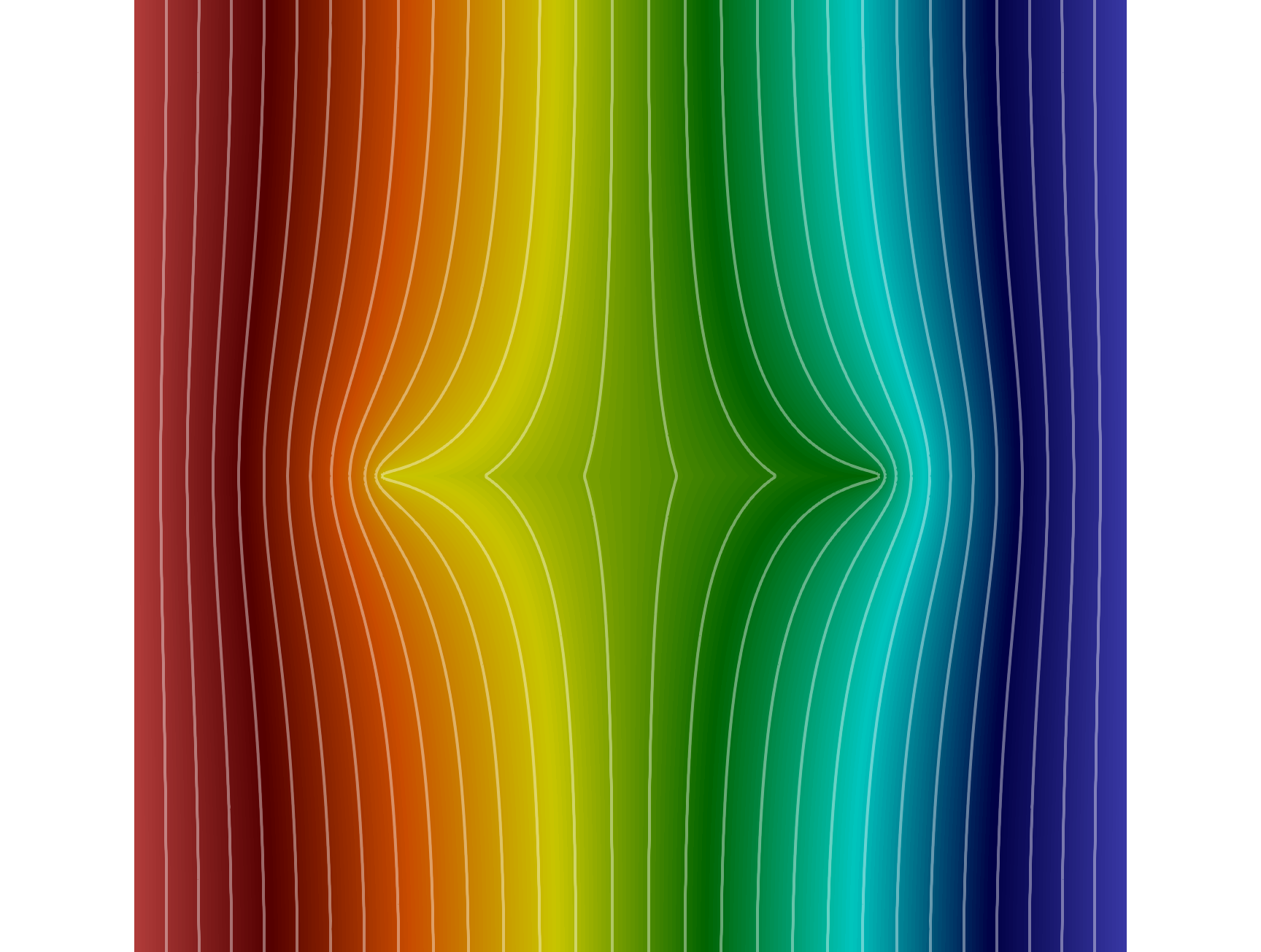
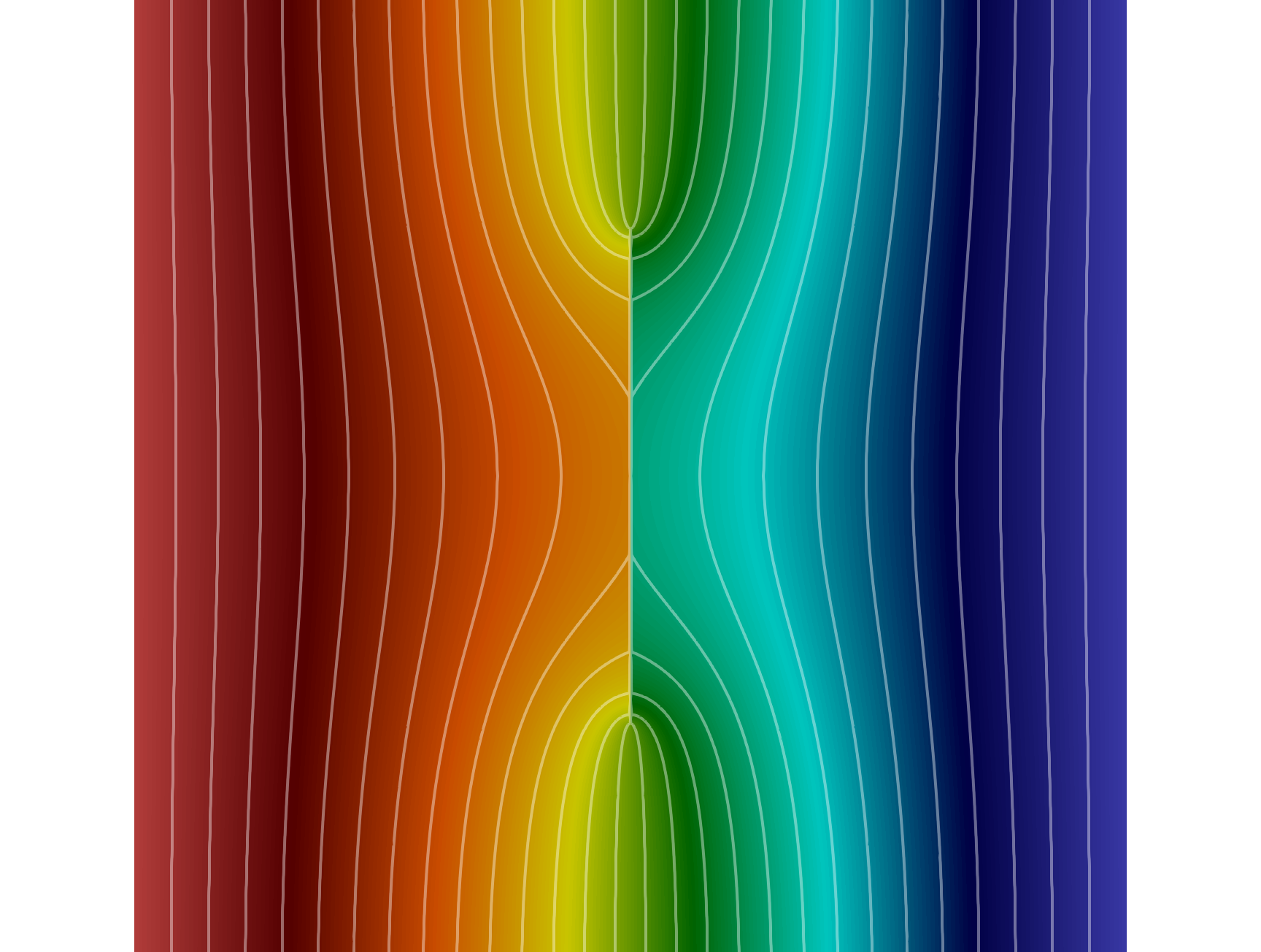
Figure 1. Example 1. Left: Domain and boundary conditions. Middle: reference solution for conductive fractures (1a). Right: reference solution for blocking fractures (1b). Color range: (0, 1). Thirty uniform contour lines from 0 to 1.

We consider two meshes, see Figure 2: a coarse unfitted triangular mesh with mesh size $h=0.1$ and a refined unfitted mesh that performs 3 steps of local mesh refinements near the fractured cells using the procedure detailed in Remark 2.7. The coarse mesh has $230$ cells, while the fine mesh has $1328$ cells.

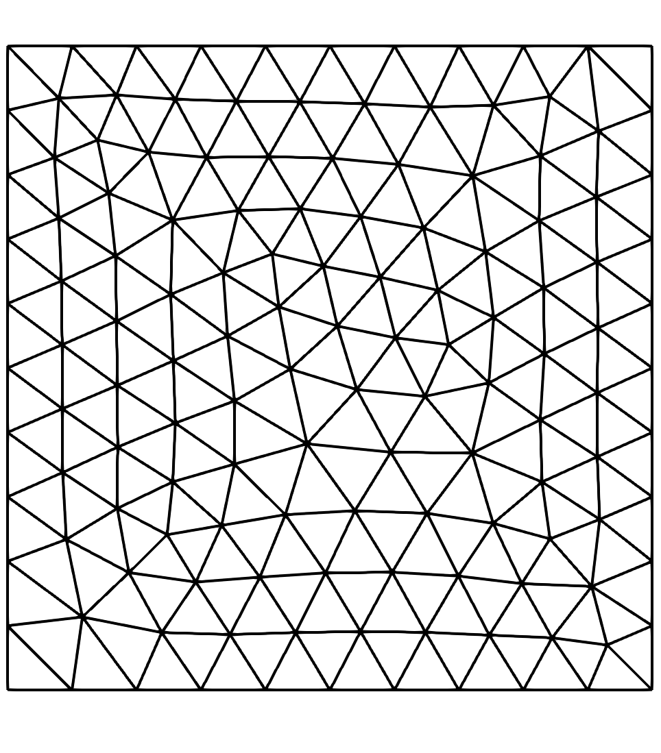
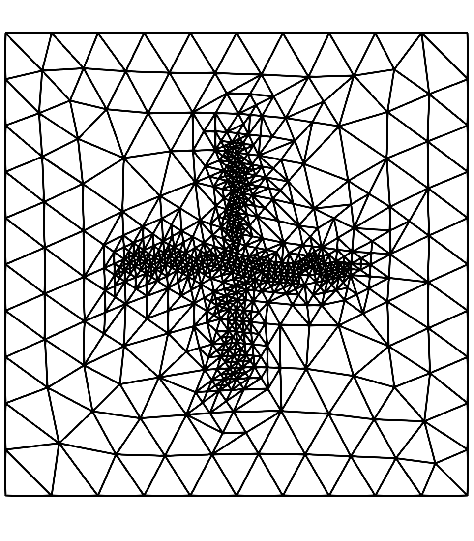
Figure 2. Example 1. Left: a coarse mesh with size $h=0.1$. Right: a locally refined mesh with $h\approx 0.1/8$ near the fractures.

We first study the role of the stabilization function $\alpha_{h}$, in particular, the effect of $s_{c}$ therein, near conductive fractures on the scheme (4). We take polynomial degree $k=0,1,2$, and vary the scaling power $s_{c}\in\{1,2,3\}$ of $\alpha_{h}$ in (4k) with $C_{c}=1$. The pressure approximations along the line $x=0.5$ are shown in Figure 3. From these figures, we observe that

• When polynomial degree $k=0$, a convergent result, comparing with reference solution, is obtained with $s=2$. For $s=1$ (smaller stabilization) the scheme does not converge as the fracture is not captured. For $s=3$ (larger stabilization) the scheme does not convergence either as it leads to a constant approximation along the fractures, which is consistent with the discussion in Remark 2.3 as too large stabilization effectively makes the pressure within conductive fractures to be a global constant for $k=0$.

• When polynomial degree $k=1$ or $k=2$, a convergent result is obtained with $s=3$. The results for $s=1$ and $s=2$ leads to locking phenomena as the effects of the fracture is not captured correctly. We note that further increase $s$ from 3 essentially leads to similar results as those with $s=3$ for this example.

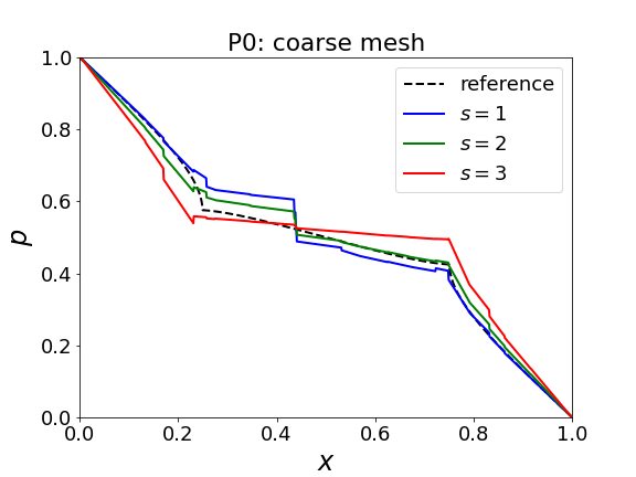
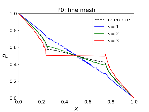
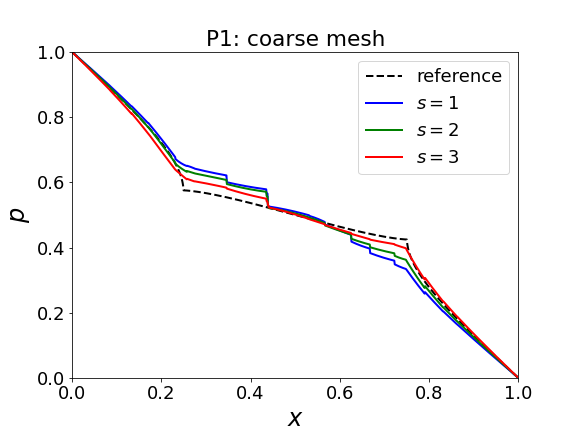
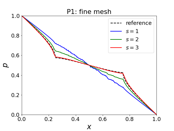
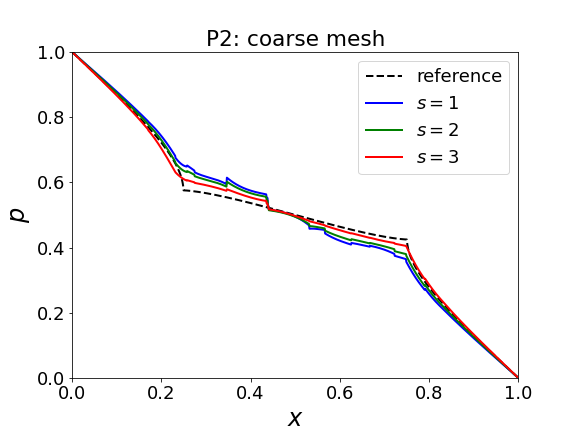
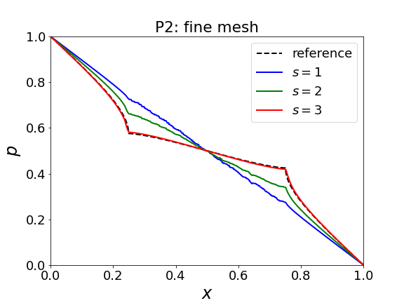
Figure 3. Example 1(a): conductive fractures. Pressure along cut line $x=0.5$ for the scheme (4) with different stabilization parameter with $s_{c}=s=1,2,3$ in (4k).

Contour plots of the pressure on the fine mesh for $k=0$ with $s_{c}=2$ and for $k=1,2$ with $s_{c}=3$ are shown in Figure 4. We observe these results are qualitatively similar to the reference solution in the middle of Figure 2.

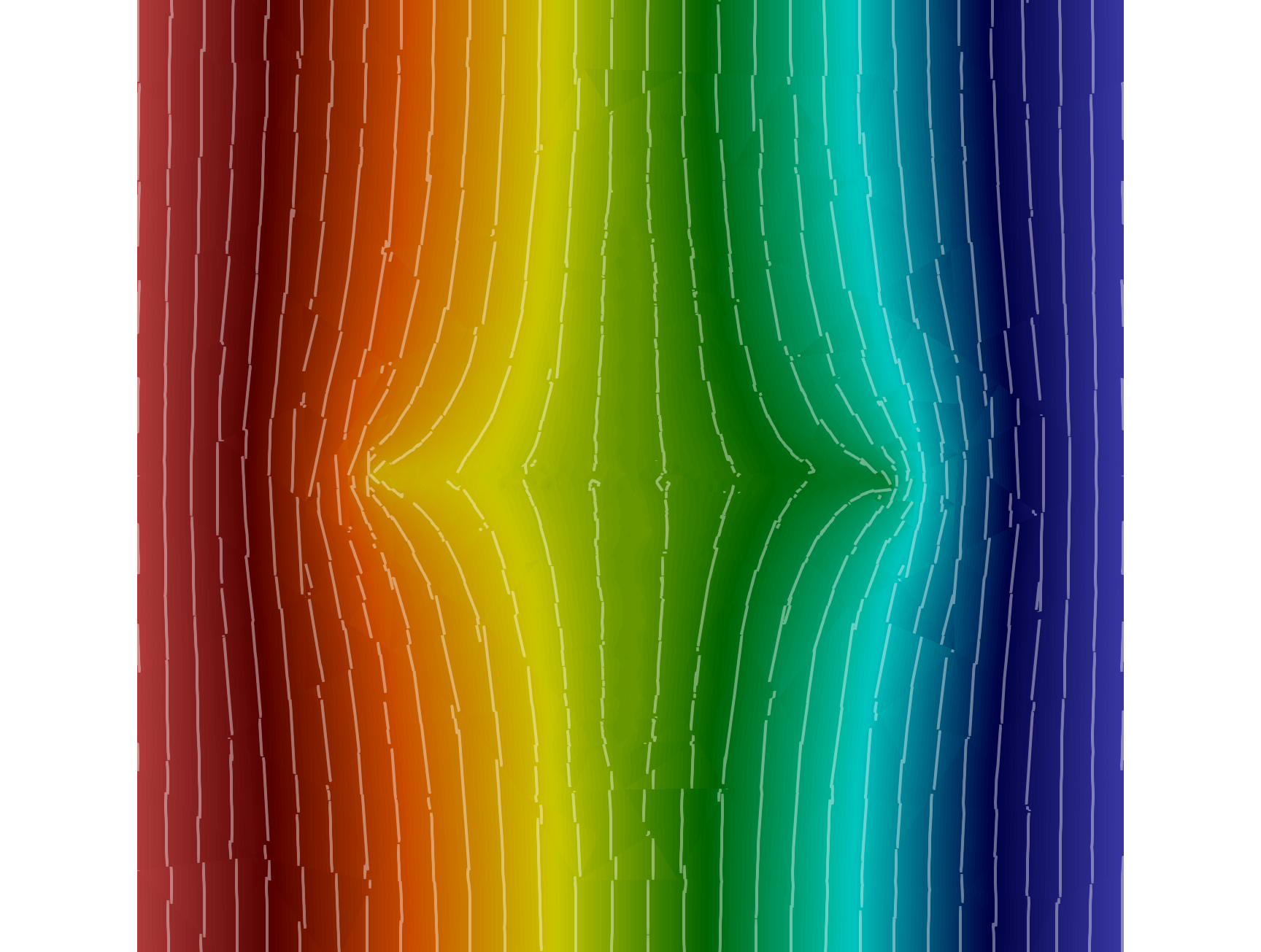
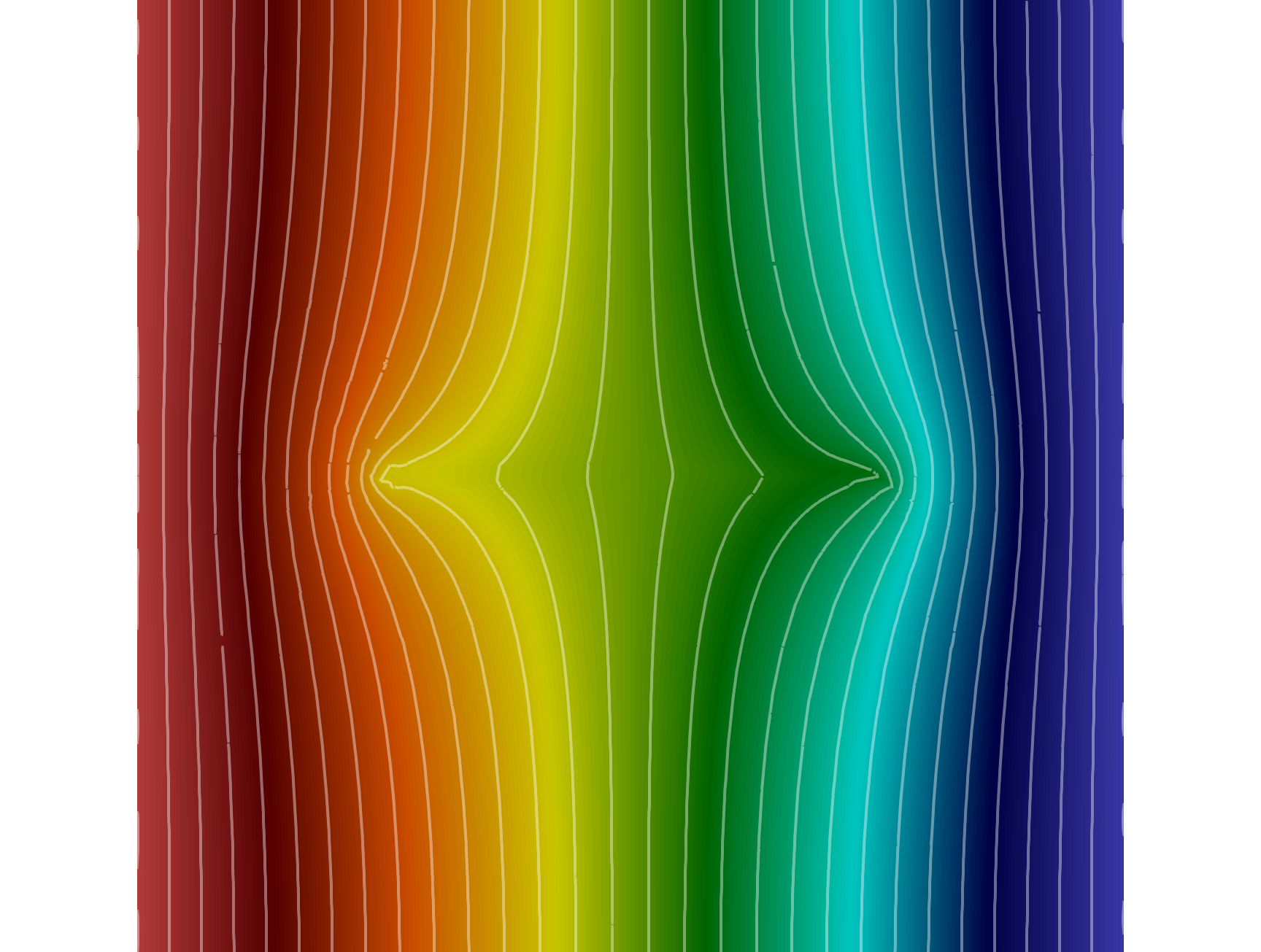
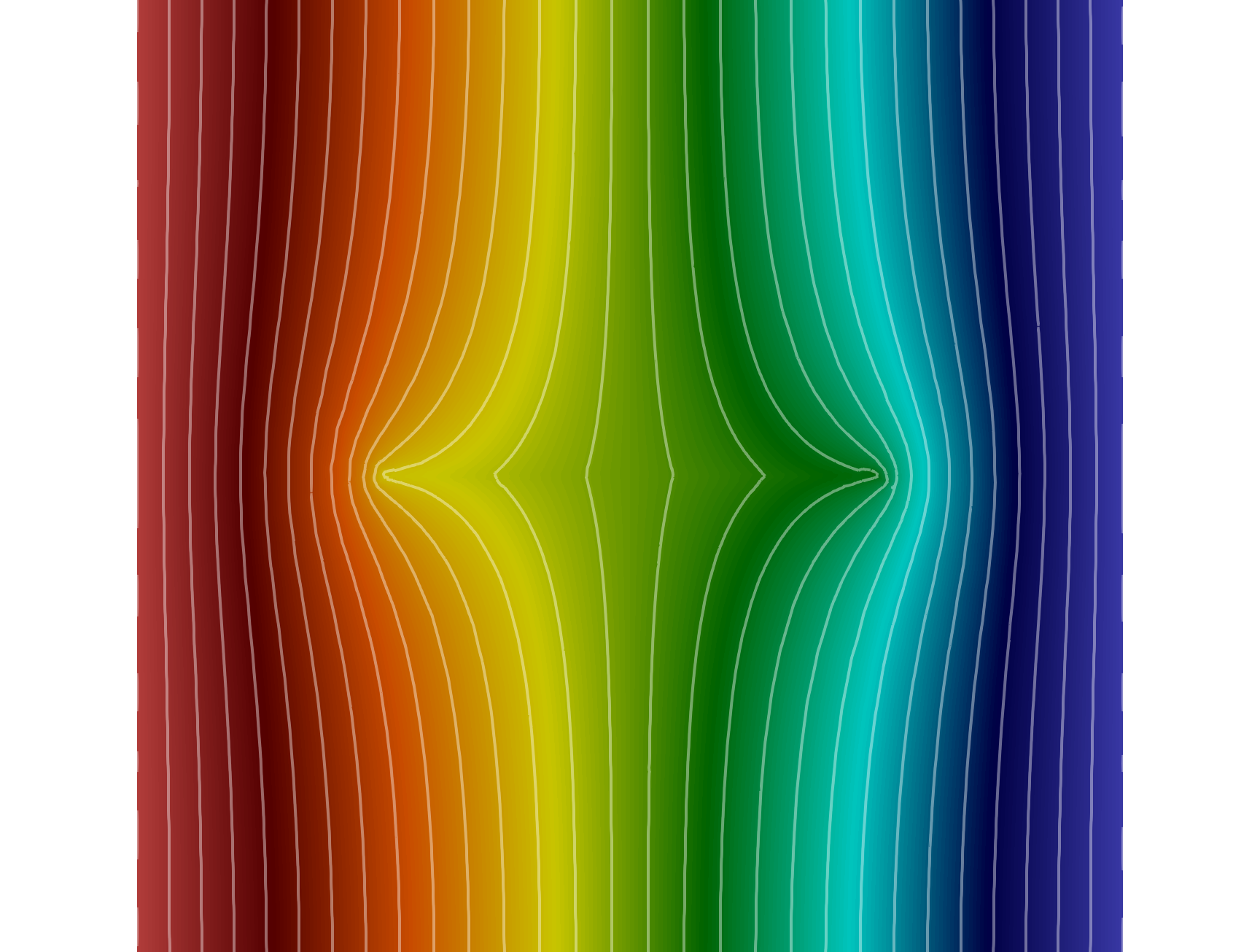
Figure 4. Example 1(a): conductive fractures. Pressure contour for $k=0,s=2$ (left), $k=1,s=3$ (middle), and $k=2,s=3$ (right).

We next study the performance of our scheme for the blocking fracture case. For this case, we find that taking the penalty parameter on blocking fractured cells to be the same as regular cells (i.e., $C_{b}=1$ and $s_{b}=0$) already lead to a convergent scheme, so we report results for this choice of parameters. The pressure approximations along the line $x=0.5$ for $k=0,1,2$ on the coarse and fine meshes are shown in Figure 5. Convergence to the reference solution is observed for all cases as mesh refines.

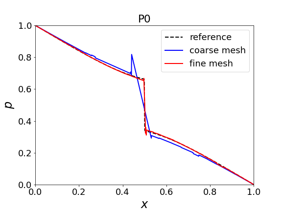
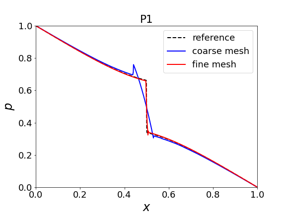
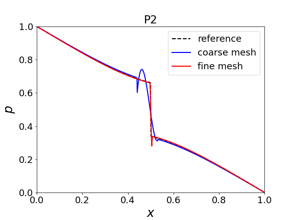
Figure 5. Example 1(b): Pressure along cut line $x=0.5$ for the scheme (4) for the blocking fracture case.

Contour plots of the pressure on the fine mesh are shown in Figure 6. We again observe these results are qualitatively similar to the reference solution in the right of Figure 2.

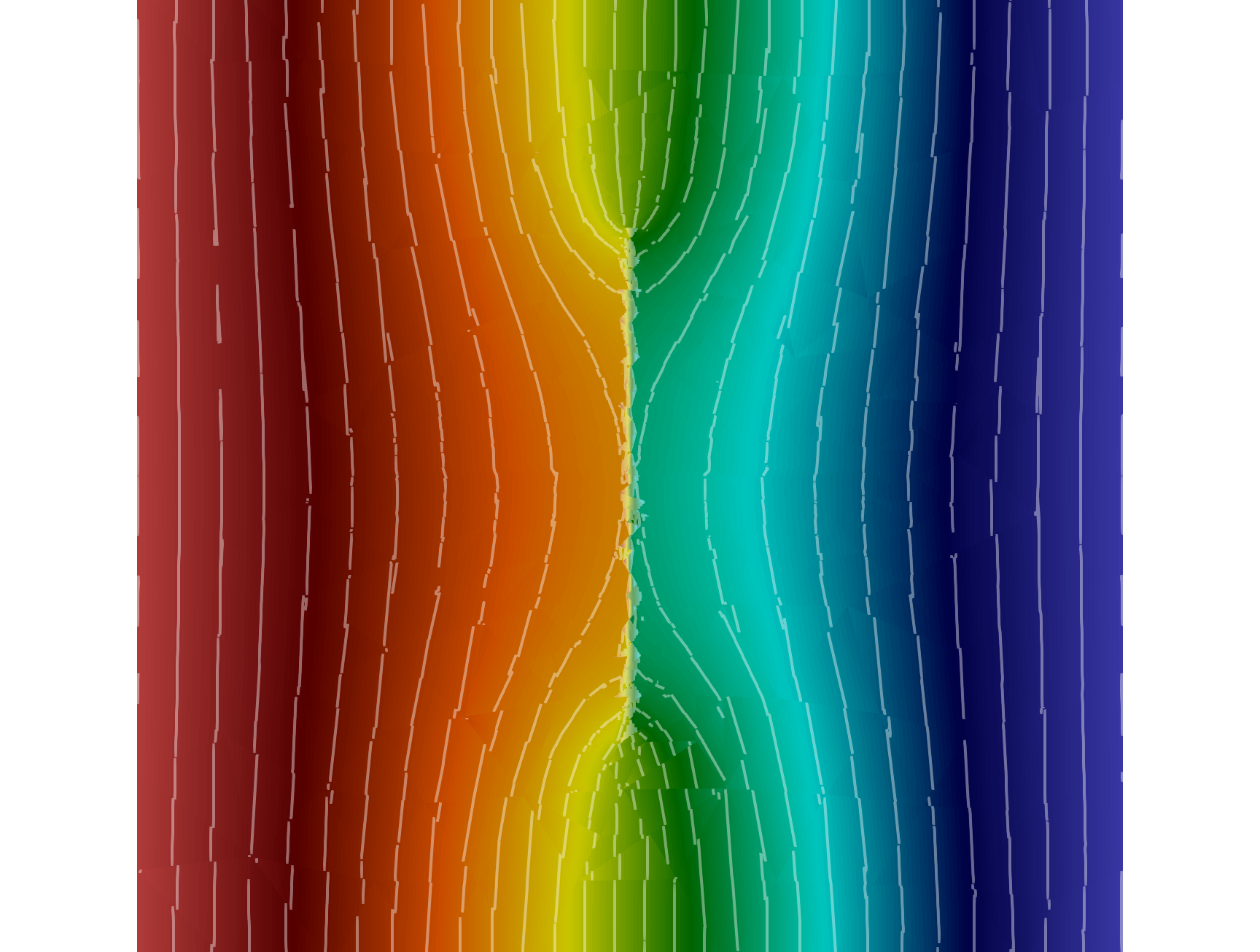
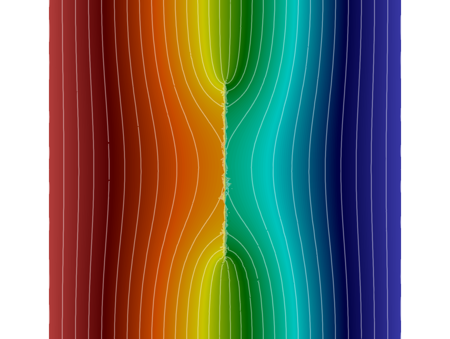
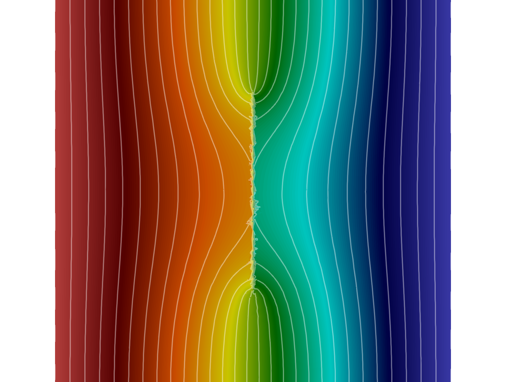
Figure 6. Example 1(b): Pressure contour for $k=0$ (left), $k=1$ (middle), and $k=2$ (right).

Example 2: Complex fracture network in 2D

This test case considers a small but complex fracture network that includes eight conductive fractures and two blocking fractures. The domain and boundary conditions are shown in Figure 7 (red represents conductive fractures, blue represents blocking fractures). All fractures are represented by line segments, and the exact coordinates for the fracture positions can be found in [37, Appendix C]. The fracture thickness is $\epsilon=10^{-4}$ for all fractures, and permeability is $k_{i}=10^{4}$ for all fractures except for fractures 4 and 5 which are blocking fractures with $k_{i}=10^{-4}$ . We consider two subcases (a) and (b) with a pressure gradient which is predominantly vertical and horizontal respectively.

Figure 7. Benchmark 3: computational domain and boundary conditions.

We consider two meshes, see Figure 8: a coarse triangular mesh with mesh size $h=0.1$ and a refined mesh that performs 3 steps of local mesh refinements near the fractures using the procedure detailed in Remark 2.7. The coarse mesh has $230$ cells, while the fine mesh has $1380$ cells.

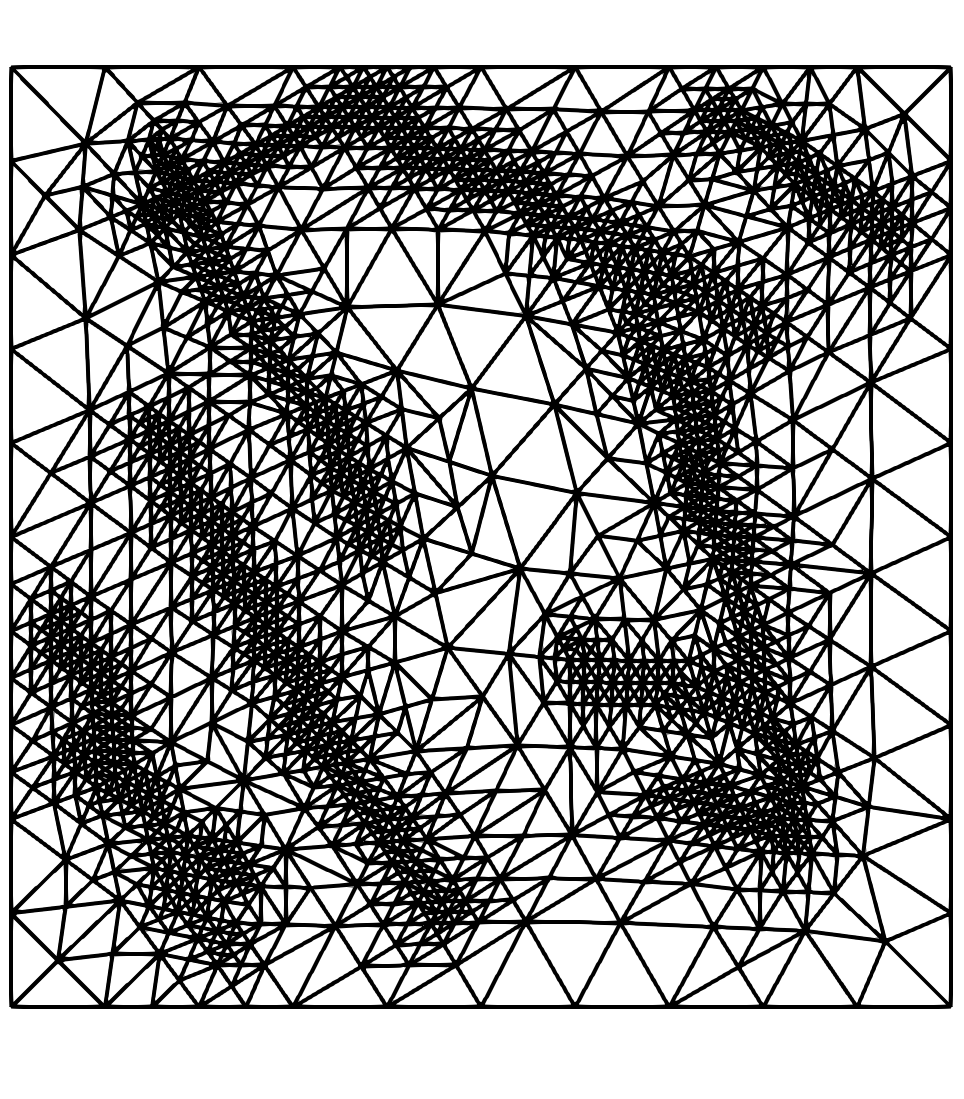
Figure 8. Example 2. Left: a coarse mesh with size $h=0.1$. Right: a locally refined mesh with $h\approx 0.1/8$ near the fractures.

We take polynomial degree $k=0,1,2$. As suggested from the previous example, we take penalty parameters $C_{b}=C_{c}=1$ and $s_{b}=0$, and use $s_{c}=2$ if $k=0$ and $s_{c}=3$ if $k=1,2$. The quantity of interest is the pressure approximation along the line segment $(0,0.5)--(1,0.9)$ for both cases, which are recorded in Figure 9. We observe a good convergence towards the reference solution as mesh refines for all cases.

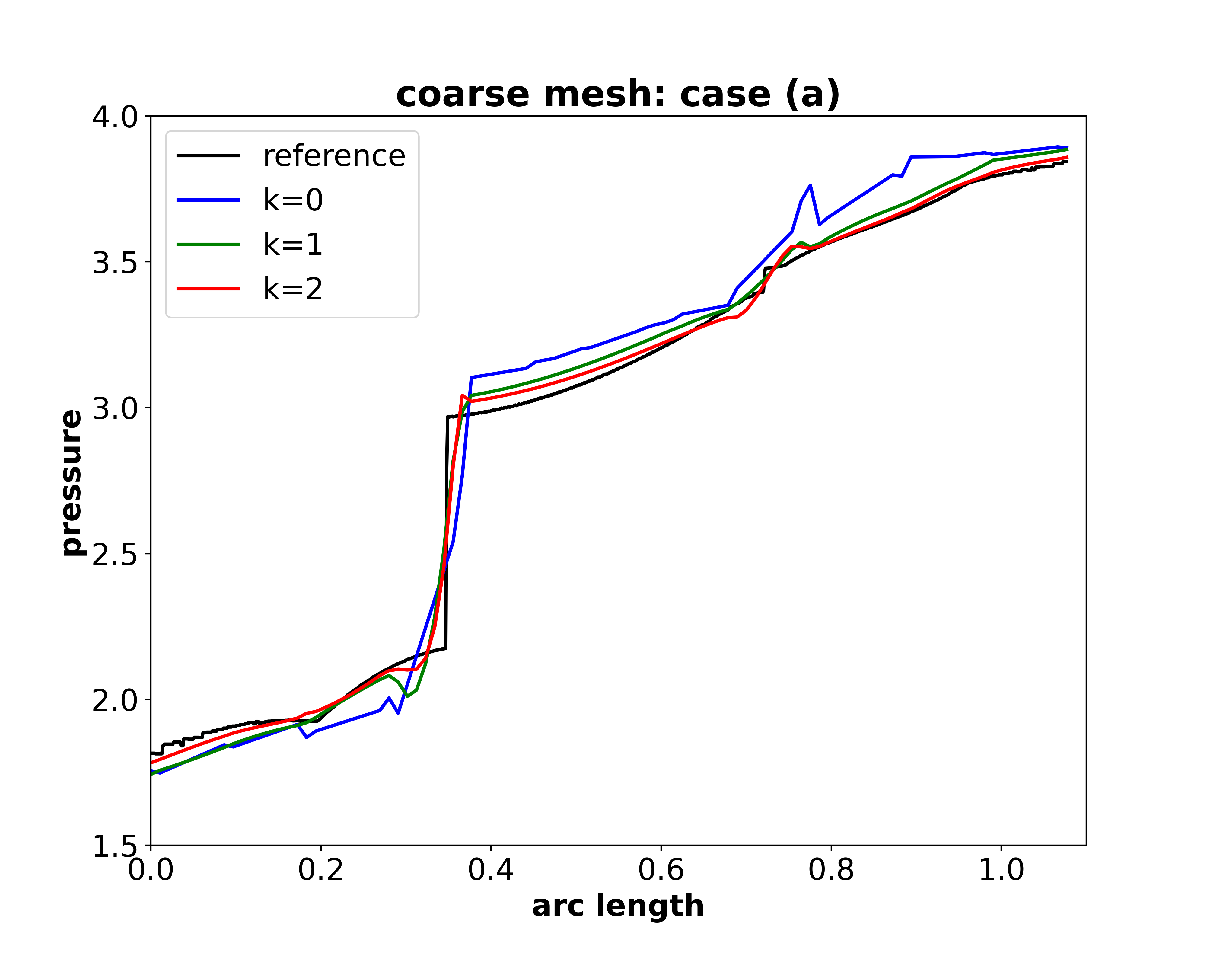
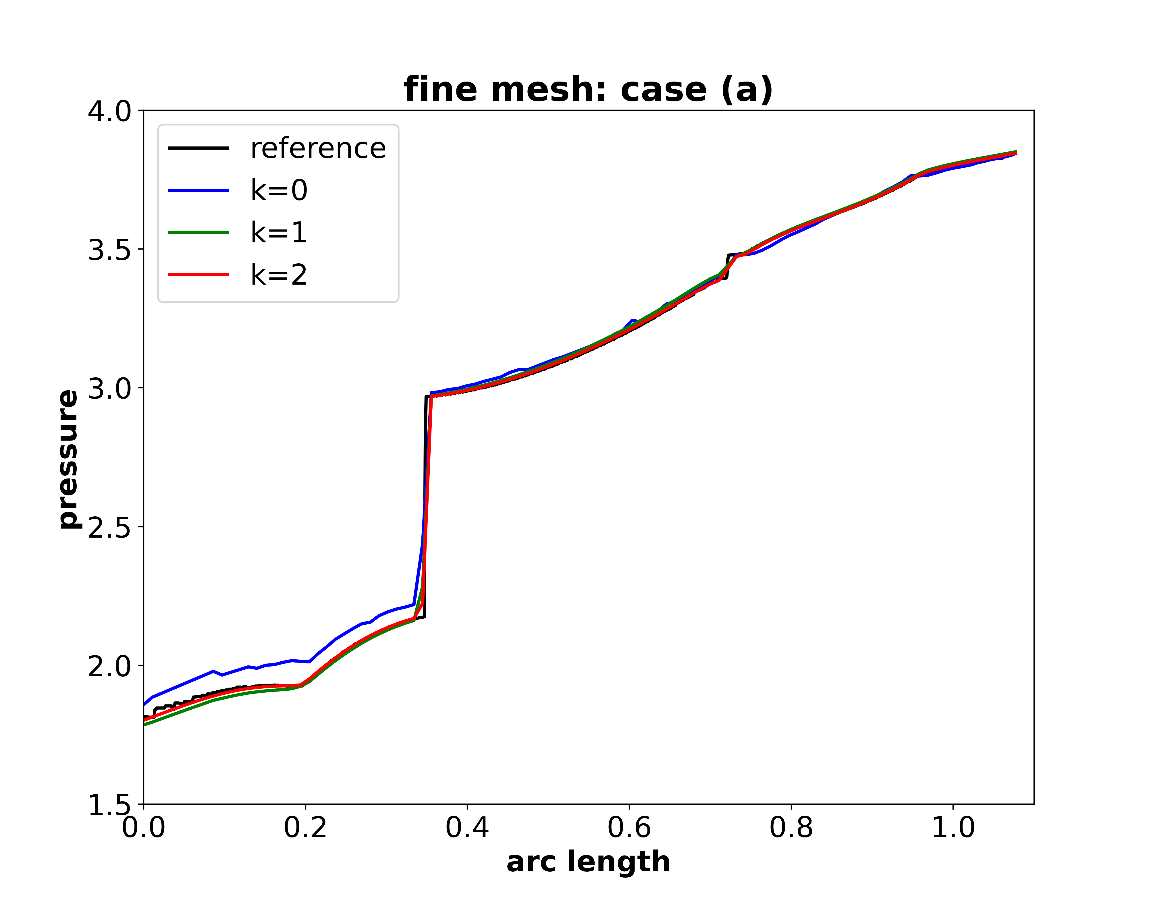
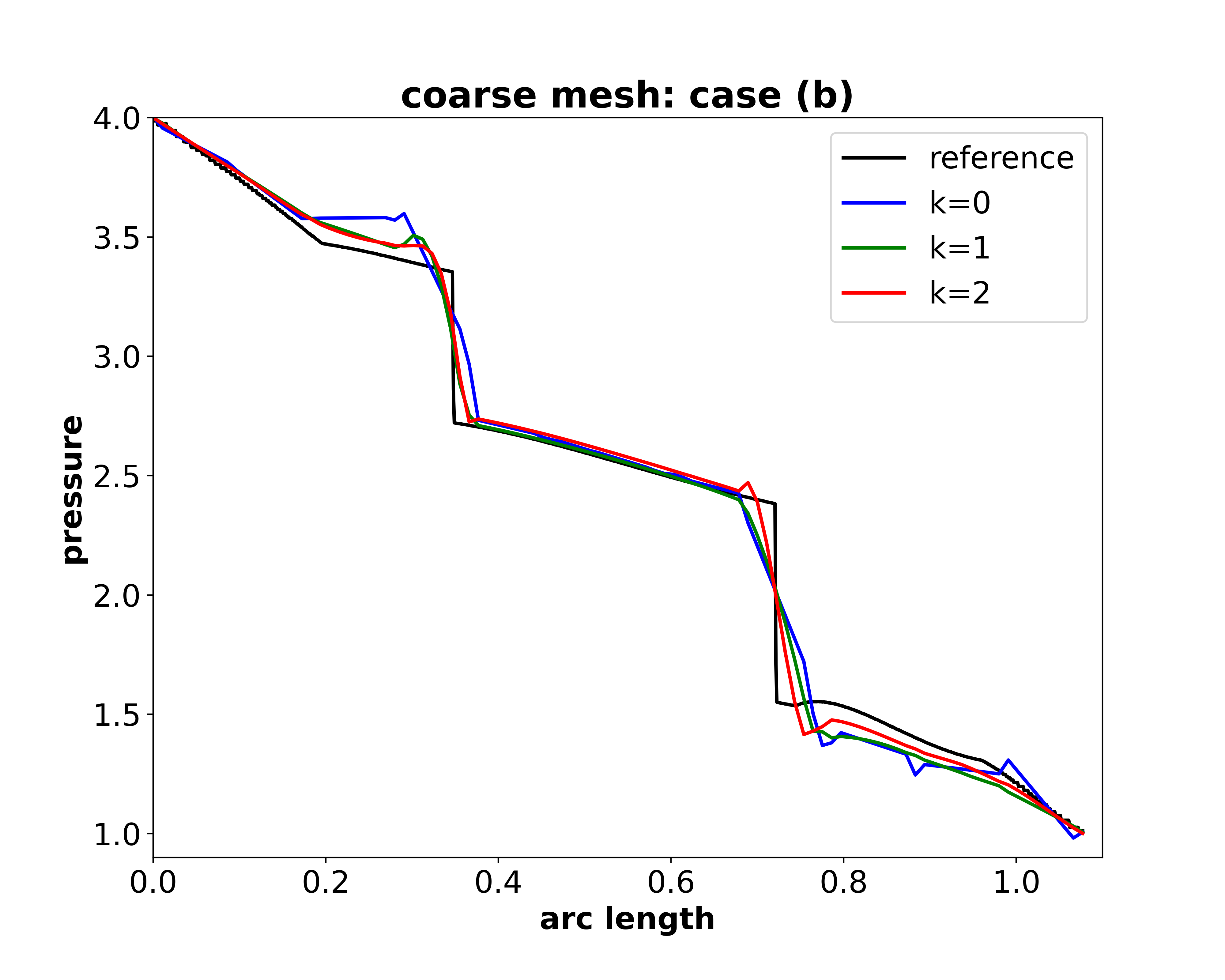
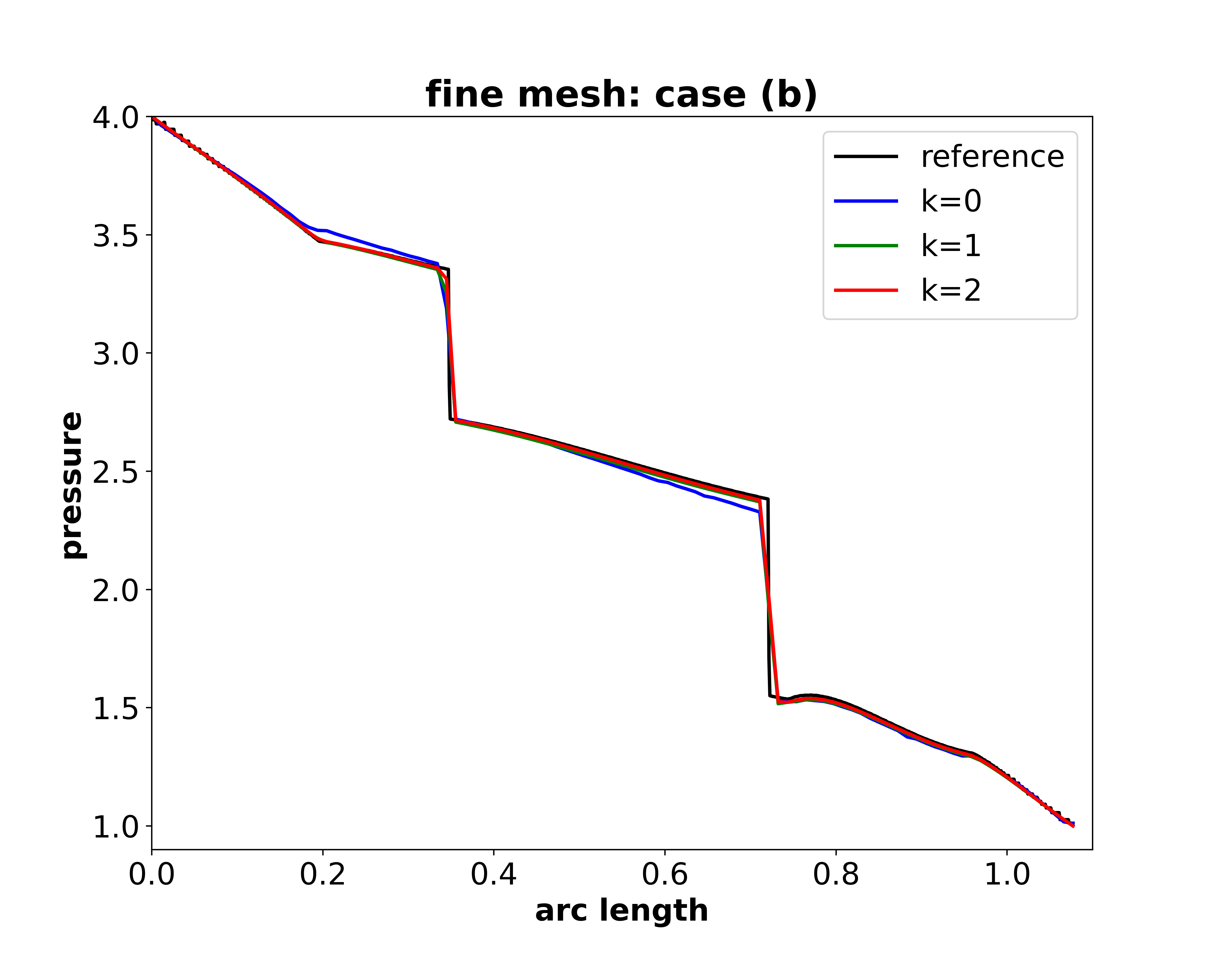
Figure 9. Example 2. Pressure along line segment $(0,0.5)--(1,0.9)$ for the scheme (4) on two meshes. Top row: case (a); Bottom row: case (b).

Contour plots of the pressure on the fine mesh are shown in Figure 10, which are consist with the results in the literature [37].

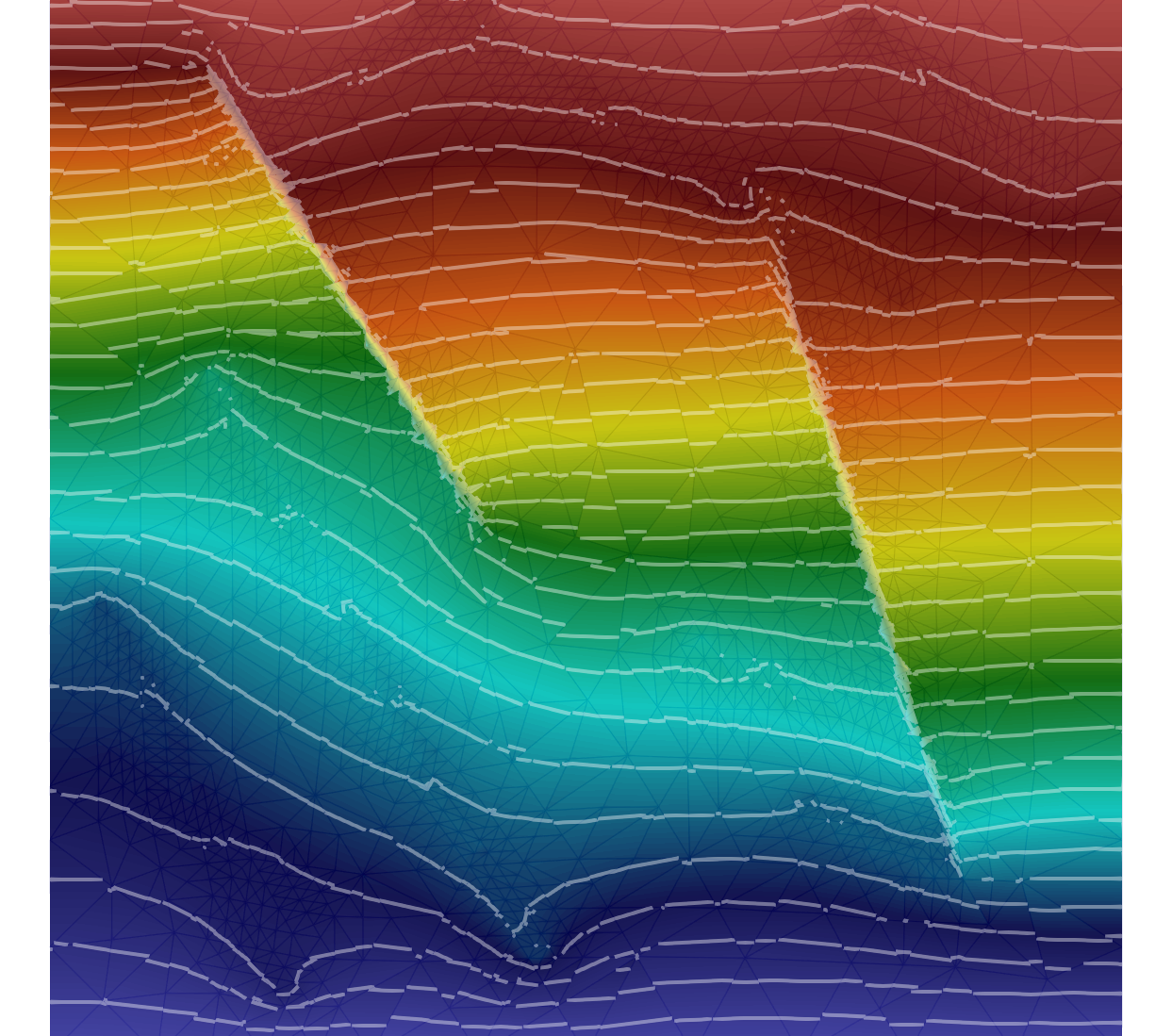
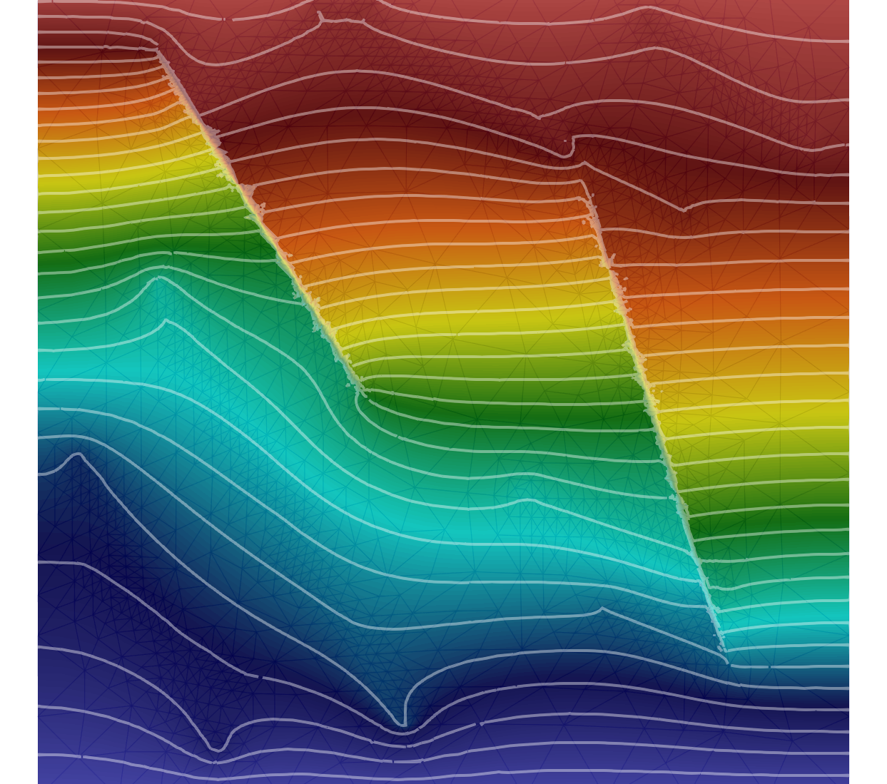
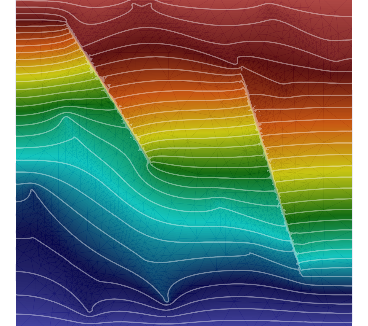
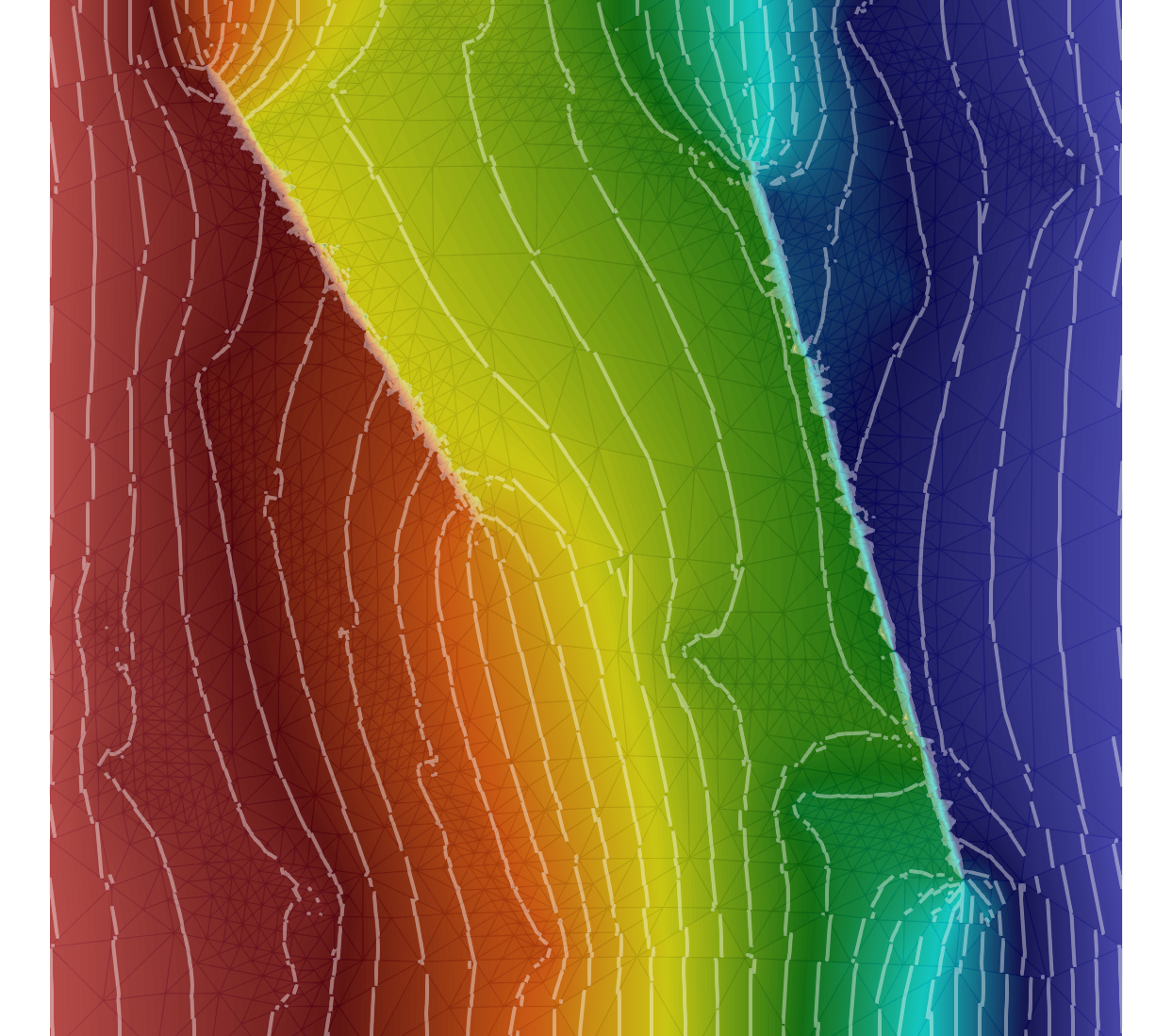
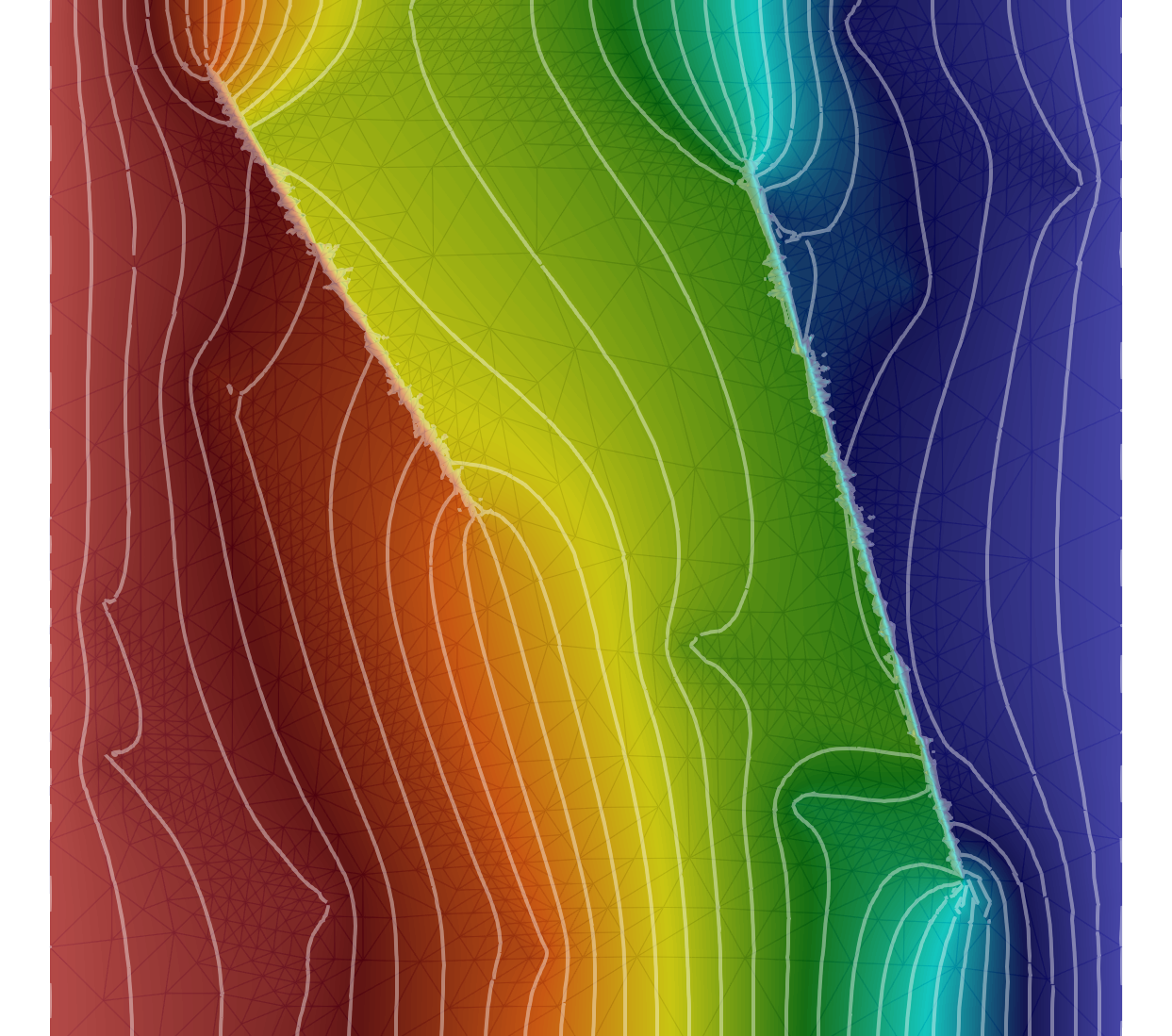
Figure 10. Example 2. Pressure contour for $k=0$ (left), $k=1$ (middle), and $k=2$ (right). Color range: (0,1). Thirty uniform contour lines from 0 to 1.

Example 3: a Realistic Case in 2D

We consider a real set of fractures from an interpreted outcrop in the Sotra island, near Bergen in Norway. The setup is adapted from [37, Benchmark 4]. The domain along with boundary conditions is given in Figure 11. The size of the domain is 700 $m$ $\times$ 600 $m$ with uniform scalar permeability $\mathbb{K}_{m}=10^{-14}m^{2}$. The set of fractures is composed of 63 line segments with thickness $\epsilon=10^{-2}m^{2}$. The exact coordinates for the fracture positions are provided in the git repository https://git.iws.uni-stuttgart.de/benchmarks/fracture-flow. Three subcases will be considered: (a) all conductive fractures with permeability $k_{c}=10^{-8}m^{2}$, (b) all blocking fractures with permeability $k_{b}=10^{-20}m^{2}$, and (c) 9 blocking fractures with $k_{b}=10^{-20}m^{2}$ and 54 conductive fractures with $k_{c}=10^{-8}m^{2}$. Location of the blocking/conductive fractures for case (c) are marked in red/blue in the right panel of Figure 12. We note that while case (a) has been extensively studied, see e.g. [37]. The other two cases are new.

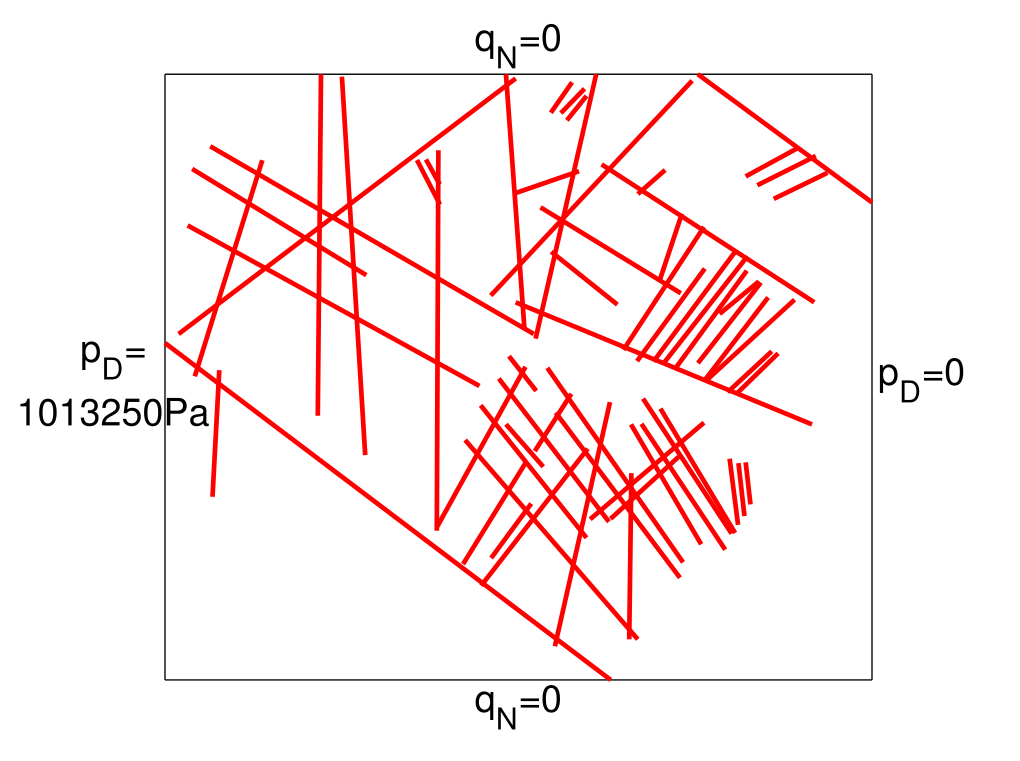
Figure 11. Example 3: Computational domain and boundary conditions.

Here we run simulation on a non-dimensional setting to avoid extreme values where the domain is scaled back to be $\Omega=(0,1)\times(0,6/7)$, matrix permeability $\mathbb{K}_{m}=1$, and inflow pressure boundary condition $p_{D}=1$ on the left boundary. We consider our scheme (4) with polynomial degree $k=0,1,2$ on an unfitted mesh obtained from a uniform triangular mesh with $h=0.01$ by performing two steps of local mesh refinements around the fractured cells; see left of Figure 12. The mesh has about $154k$ total triangular cells, and about $27.5k$ fractured cells, which further split to $5.5k$ blocking fractured cells and $22k$ conductive fractured cells for case (c).

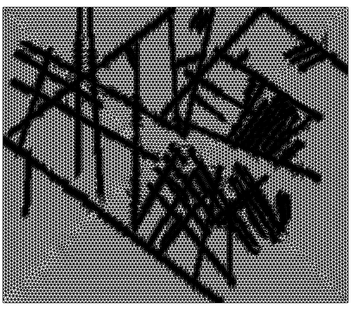
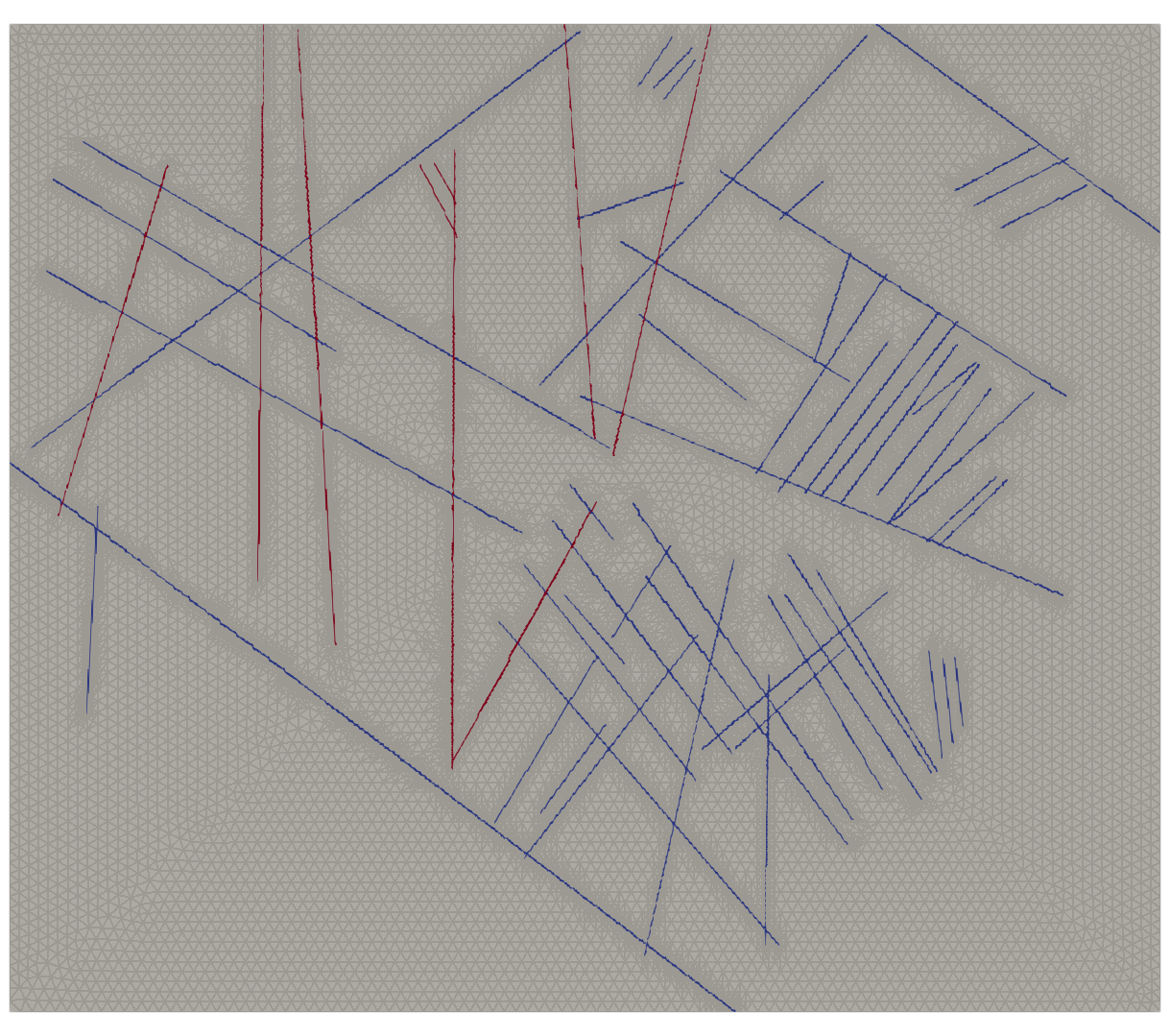
Figure 12. Example 3. Left: unfitted mesh with 154,174 cells. Right: location of blocking (in red) and conductive (in blue) fractured cells for case (c).

The penalty parameters in (4k) are given in Table 1. Here due to stronger conductive/blocking effects (with permeability differs by six orders of magnitude), we need to choose the penalty parameters $s_{b}$ and $C_{c}$ differently than the previous two examples. In particular, we note that the $C_{c}$ values are tuned to make the case (a) results matching with existing work. Moreover, the stabilization on blocking fractured cells are reduced by taking $s_{b}=2$, as taking larger stabilization with $s_{b}=0$ leads to pressure leakage across blocking fractured cells.

$k$	$C_{b}$	$s_{b}$	$C_{c}$	$s_{c}$
0	1	2	6	2
1	1	2	0.08	3
2	1	2	0.16	3

Table 1. Example 3. Choice of the penalty parameters for different polynomial degree $k$.

The pressure approximations along the two lines $y=5/7$ and $x=625/700$ are recorded in Figure 13, where reference data from the Mortar-DFM scheme on a fitted mesh with about $10k$ cells reported in [37] for case (a) is also presented. We observe a good agreement with the reference data for case (a) for our schemes. Moreover, we observe very close results for $k=1$ and $k=2$ for case (b) and case (c), where the results for $k=0$ is slightly off due to coarse mesh resolution and low-order approximations. Further refining the mesh for $k=0$ leads to results closer to the $k=1,2$ cases in Figure 13.

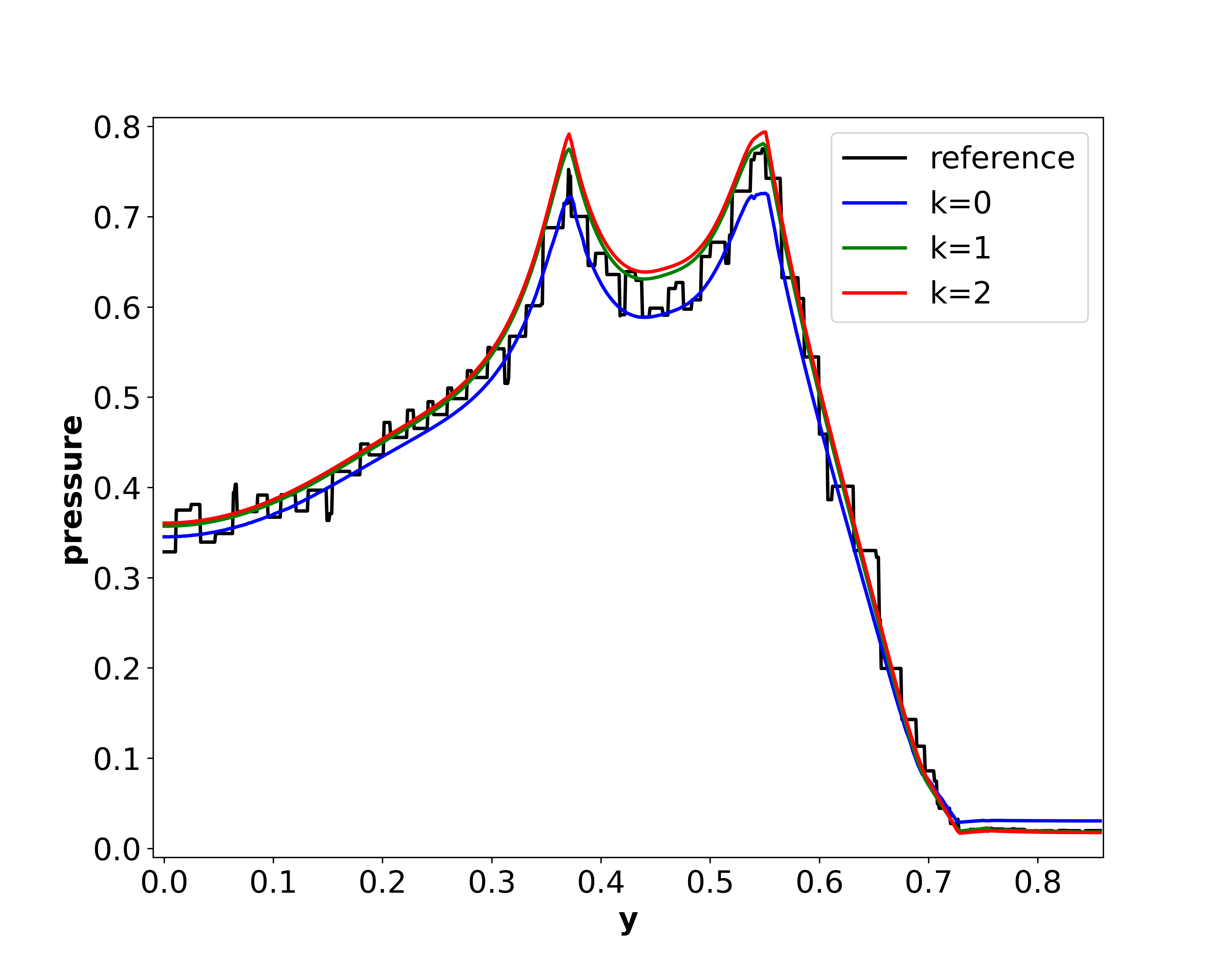
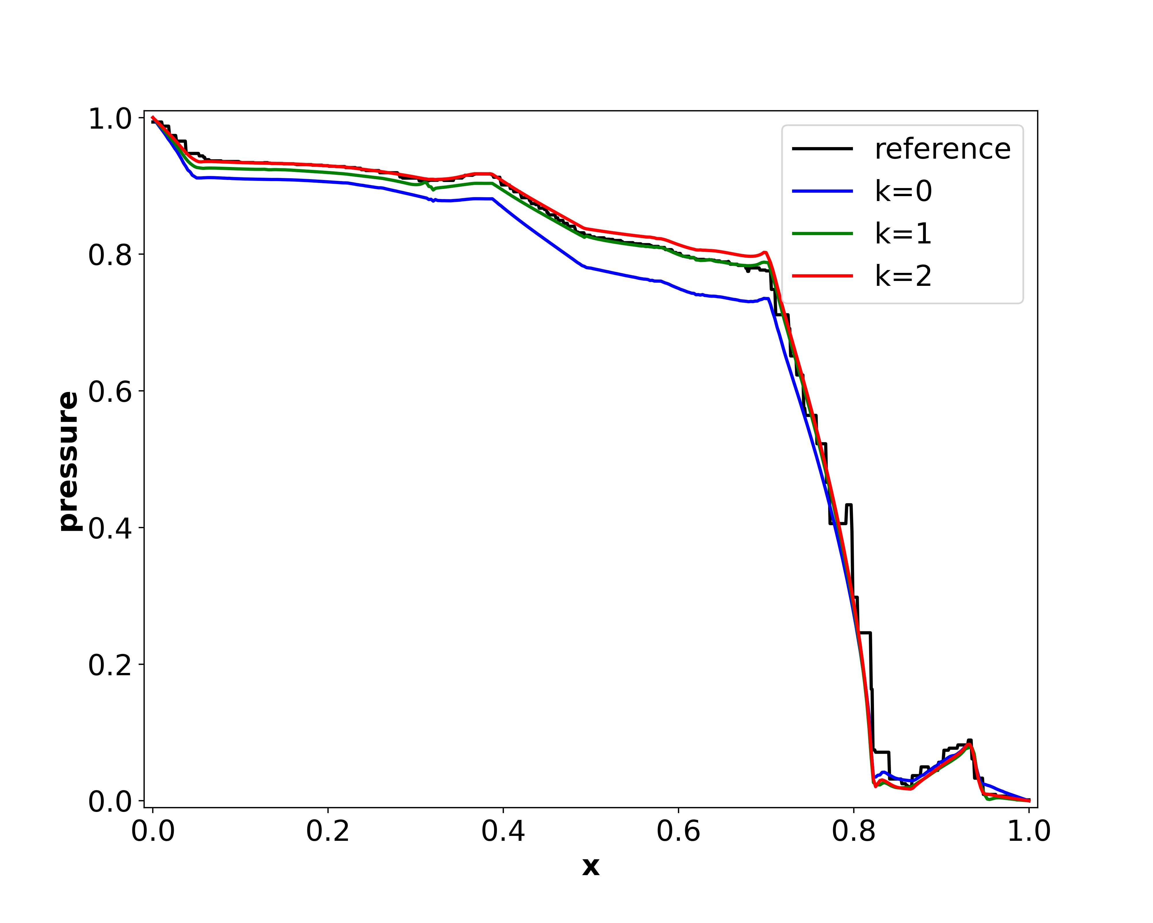
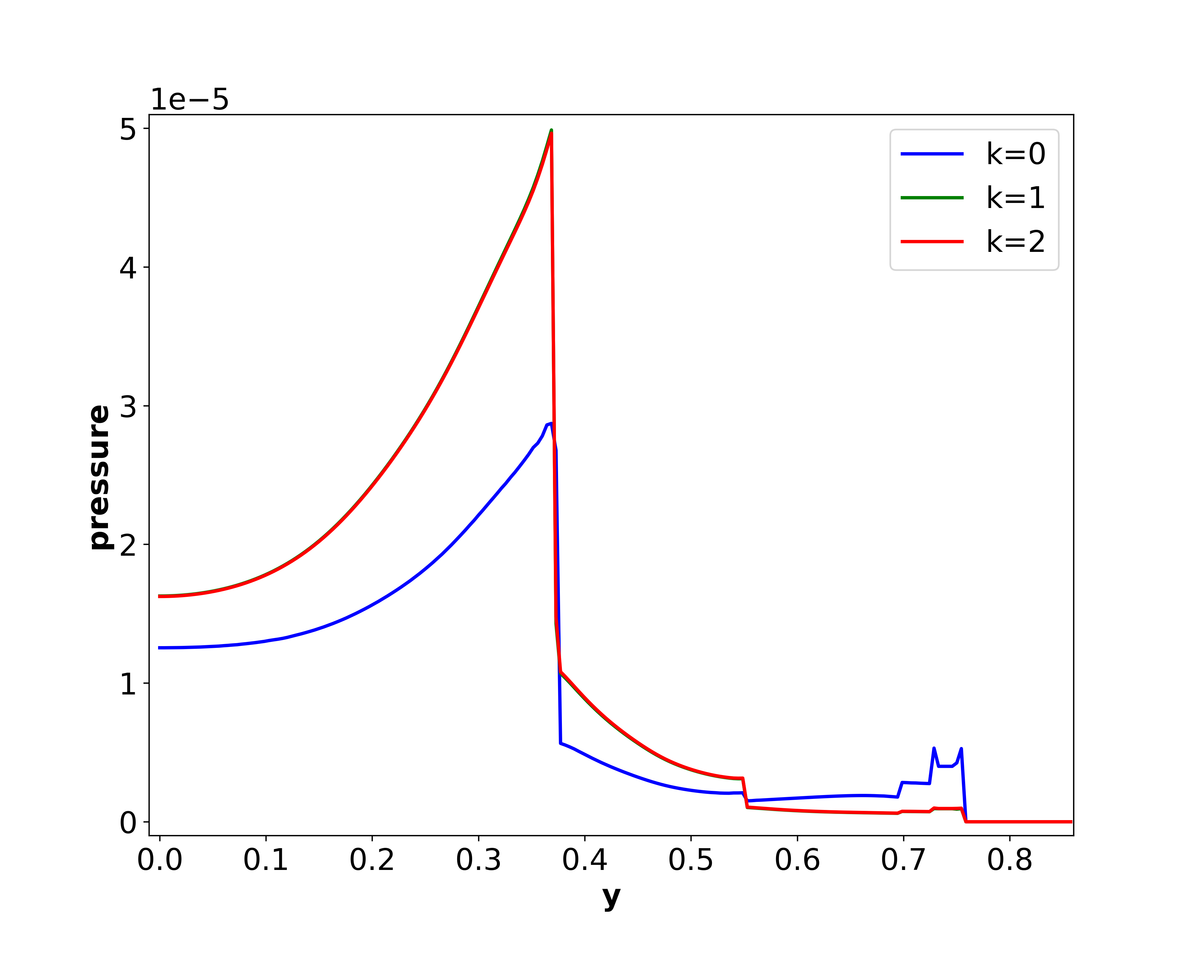
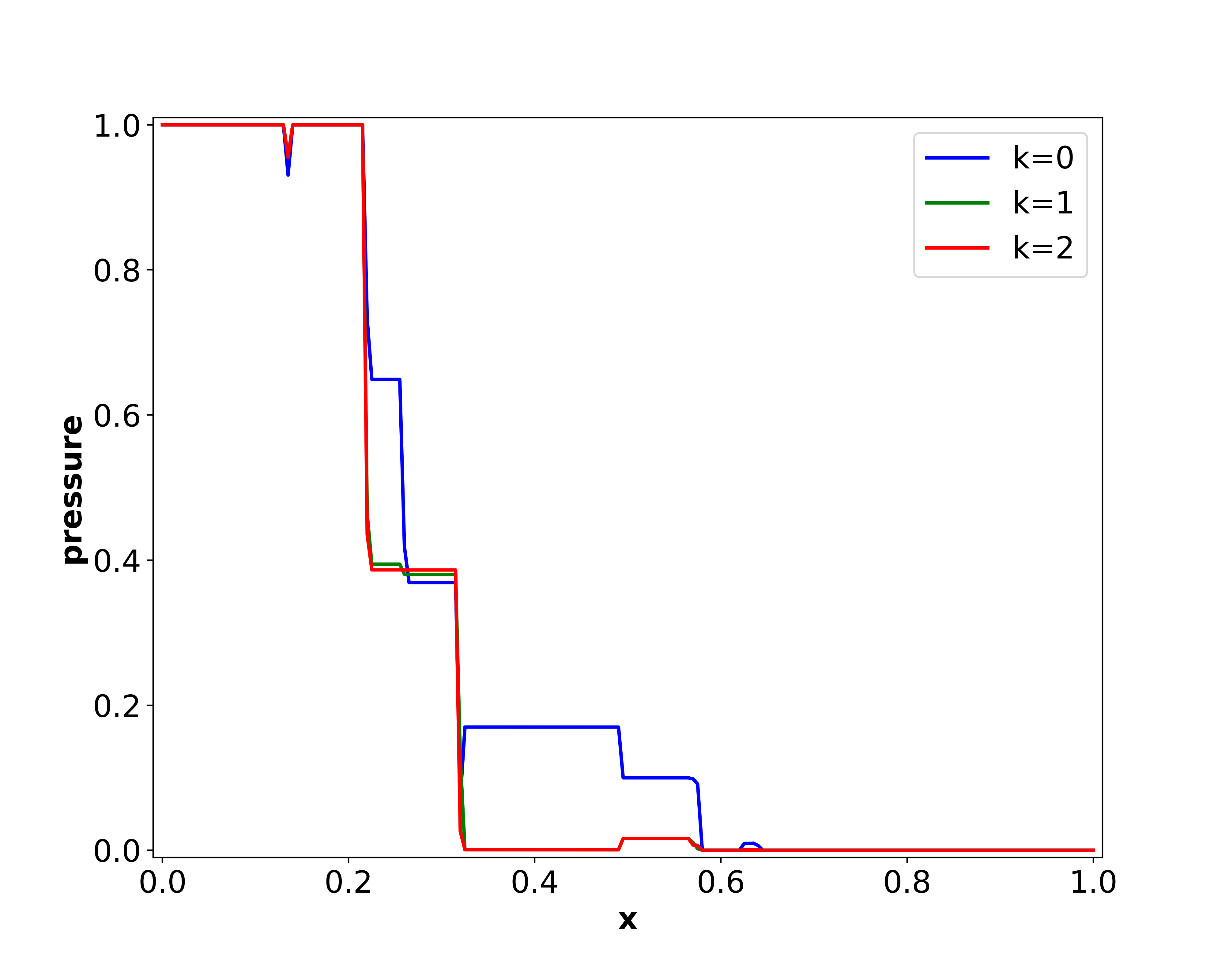
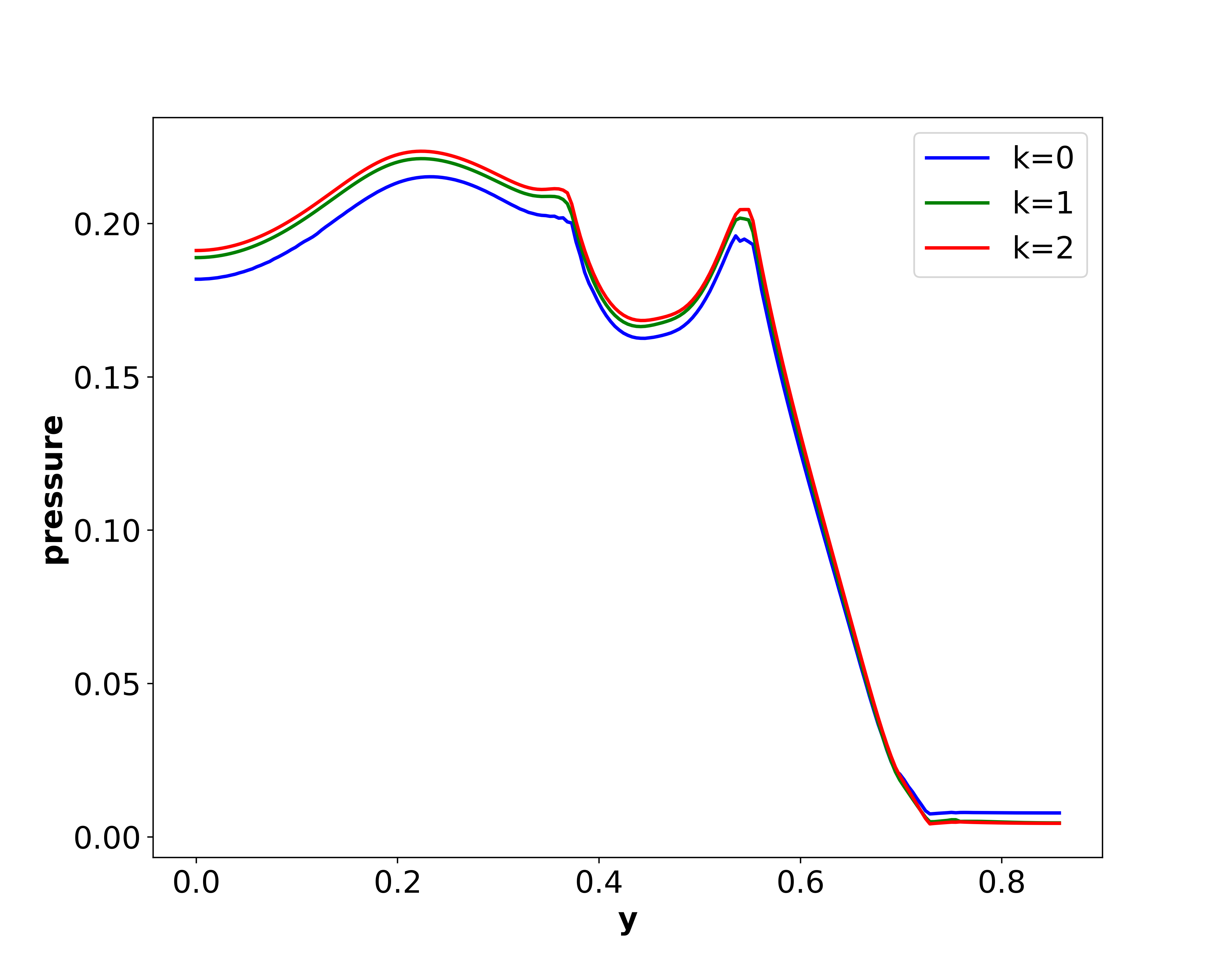
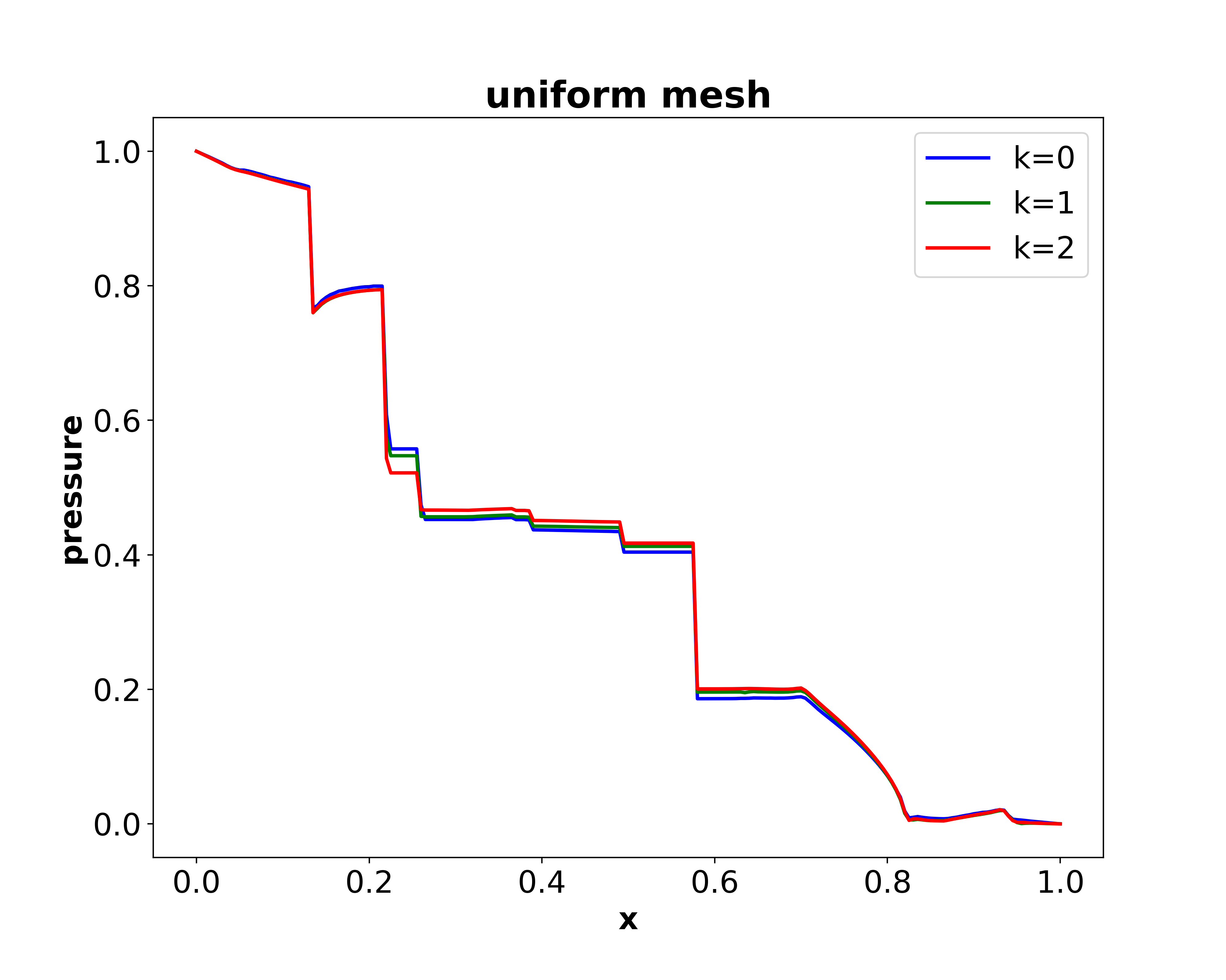
Figure 13. Example 3. Pressure along line $y=5/7$ (left column) and along line $x=625/700$ (right column). Here reference data for case (a) is the result for the Mortar-DFM scheme in [37].

Contour plots of the pressure are shown in Figure 14, where the case (a) results are again consist with those in the literature [37]. We also clearly observe the blocking effects (with discontinuous pressures) of the fractures for case (b), and the combined conductive/blocking effects of the fractures for case (c). This example confirms the ability of the proposed HDG scheme 4 in simulating realistic complex fracture networks on unfitted meshes with both conductive and blocking fractures.

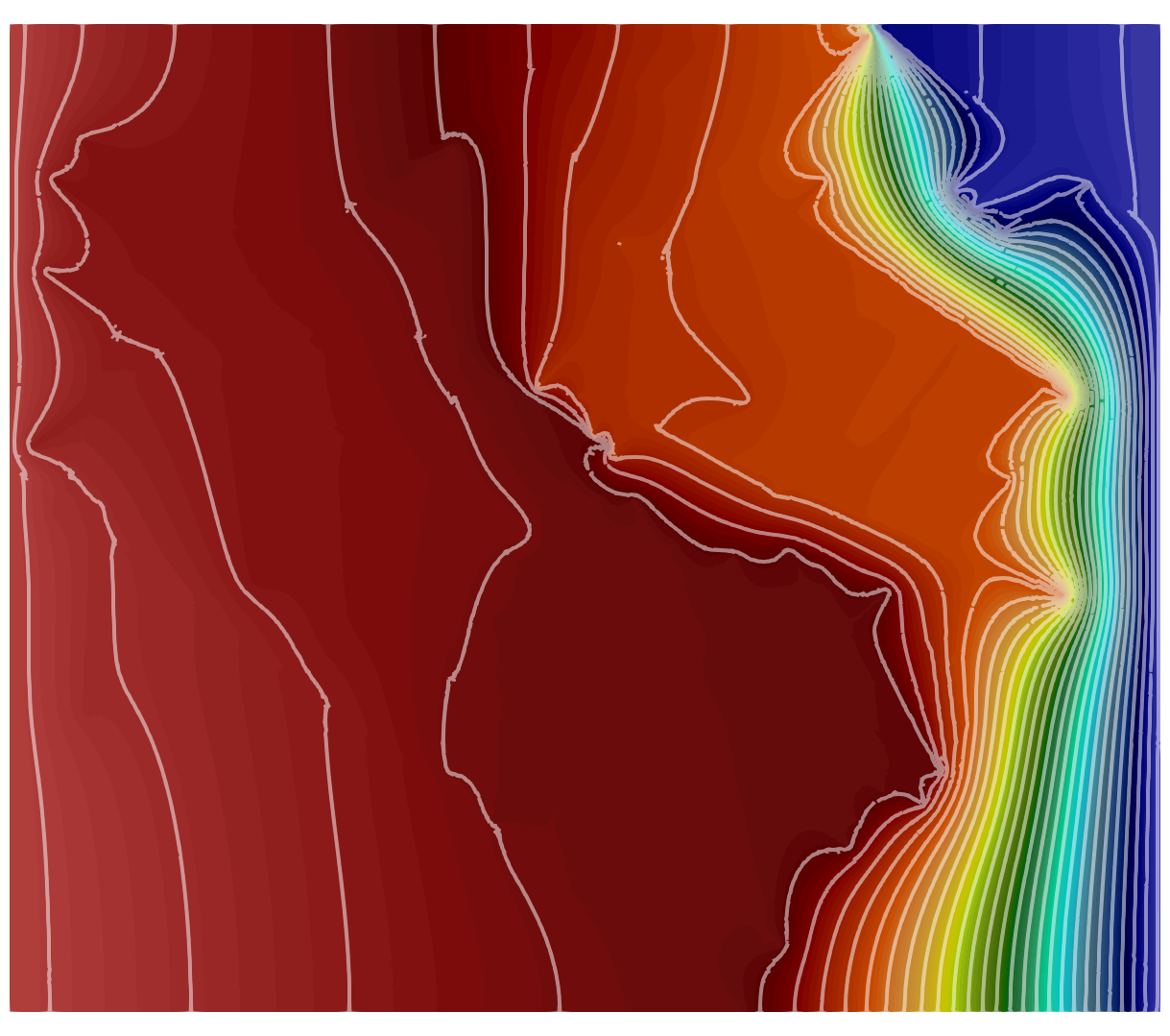
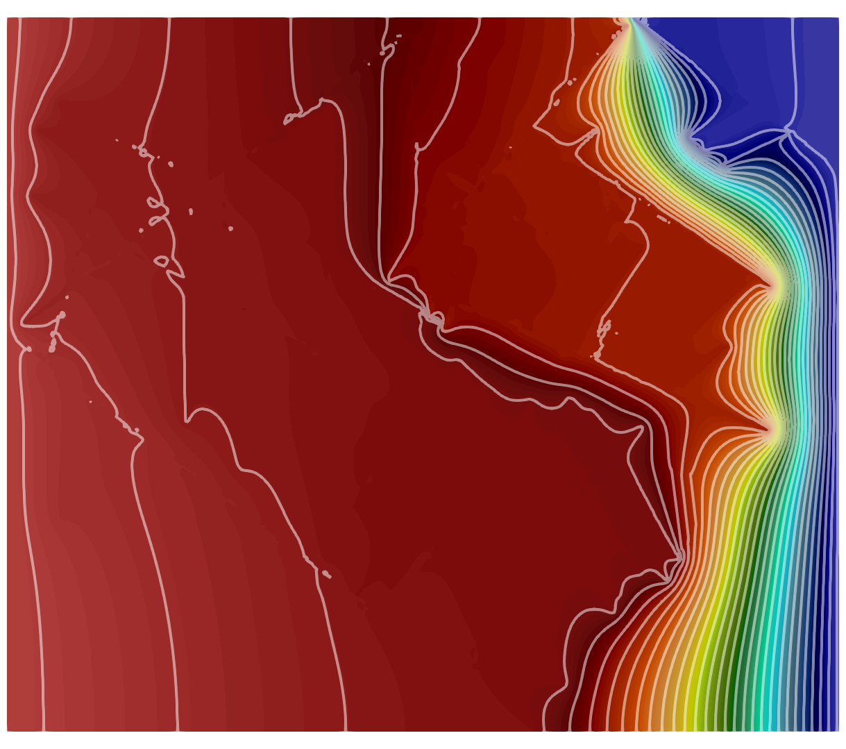
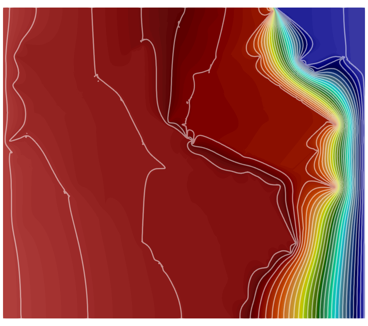
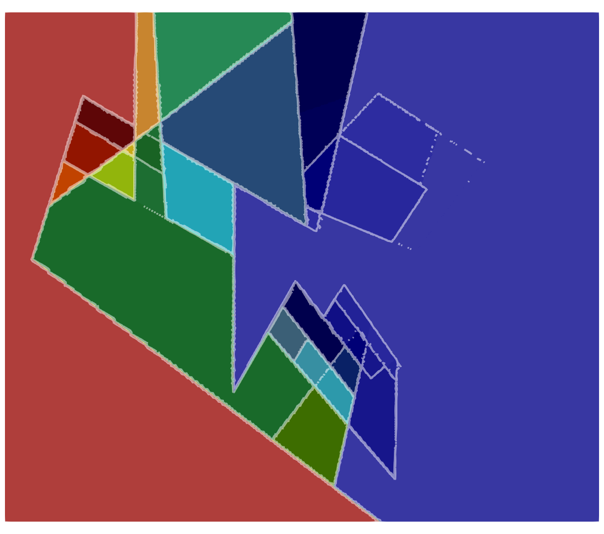
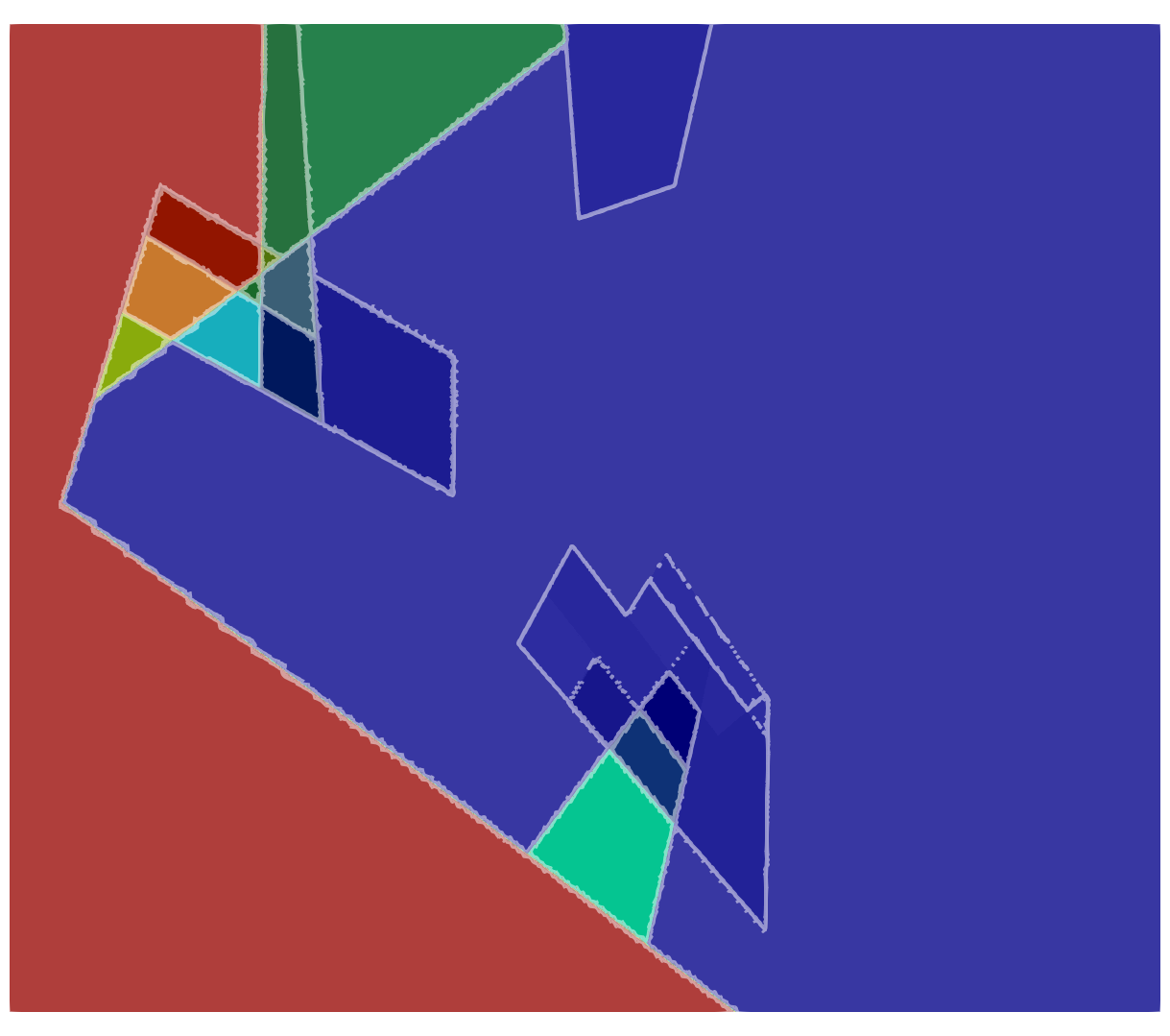
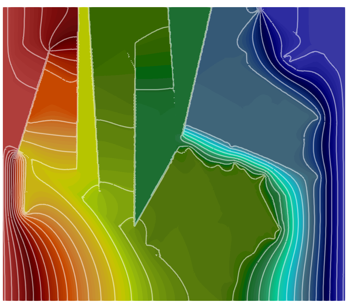
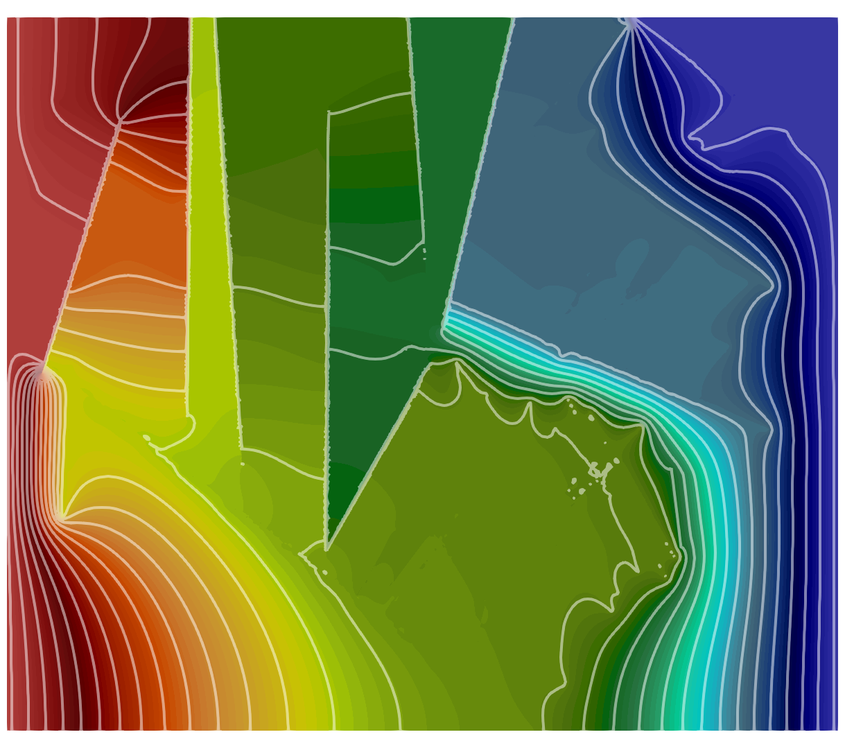
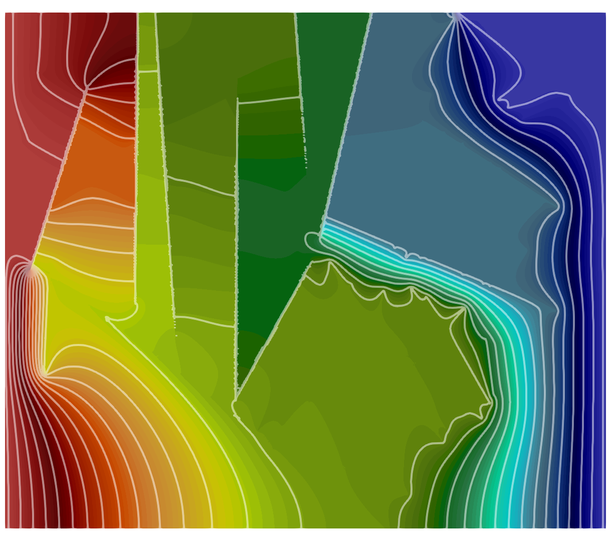
Figure 14. Example 3. Pressure contours for $k=0$ (left), $k=1$ (middle), and $k=2$ (right). Top row: case (a). Middle row: case (b). Bottom row: case (c). Color range: (0,1). Thirty uniform contour lines from 0.01 to 0.99.

Example 4: single fracture in 3D

This is the first 3D benchmark case proposed in [49]. The matrix domain $\Omega=(0,100)\times(0,100)\times(0,100)$ which is crossed by a conductive planar fracture $\Gamma_{1}$ connected by the points $(0,0,80)$, $(100,0,20)$, $(100,100,20)$, $(0,100,80)$ with a thickness of $\epsilon=10^{-2}$. The matrix permeability is heterogeneous and is taken to be $\hbox{\boldmath$K$}_{m}=10^{-6}$ when $z\geq 10$ and $\hbox{\boldmath$K$}_{m}=10^{-5}$ when $z<10$. The fracture conductivity is $k_{c}=0.1$ so that $\epsilon k_{c}=10^{-3}$. We apply the Dirichlet boundary conditions on the two boundaries

$$\Gamma_{in}:=\{0\}\times(0,100)\times(90,100),\Gamma_{out}:=(0,100)\times\{0\}\times(0,10),$$

where $p=4$ on $\Gamma_{in}$ and $p=1$ on $\Gamma_{out}$. No flow boundary conditions is used on the rest of the domain boundary.

In this example, we apply the HDG scheme (4) with degree $k=0,1,2$ on two uniform hexahedral meshes with mesh size $h=10$ (1000 cubic cells) and $h=5$ (8000 cubic cells) where we take $s_{c}=2$ and $C_{c}=1$ for $k=0$, and $s_{c}=3$ and $C_{c}=1$ for $k=1,2$ in the stabilization parameters. Here the characteristic length in (4k) is $L=100$. We plot in Figure 15 pressure along the diagonal line $(0,0,0)-(100,100,100)$ together with reference data provided in [49] which is obtained from the USTUTT-MPFA method therein on a mesh with approximately 1 million matrix elements. Good agreement with reference solution is observed for $k=1$ and $k=2$. The results for $k=0$ is slightly off, but it improves as mesh refines.

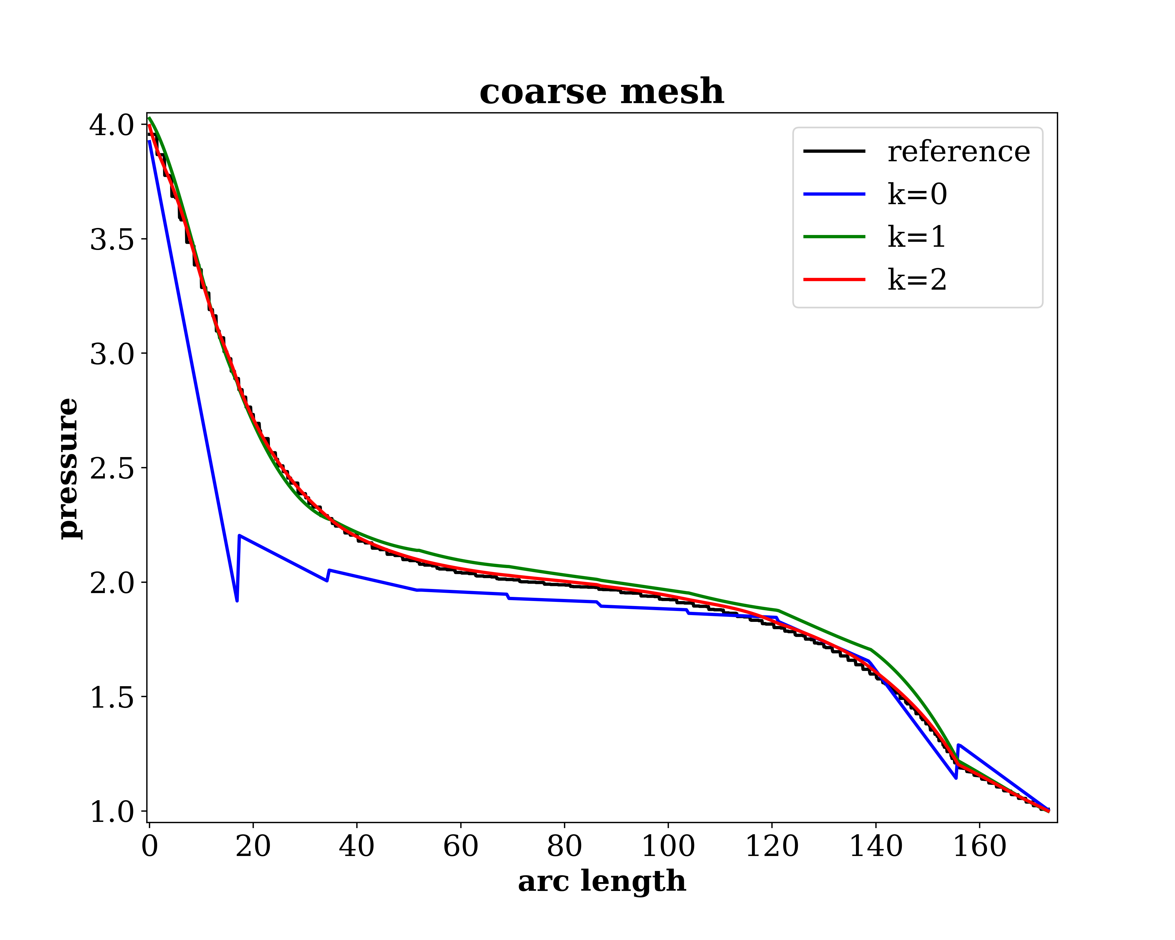
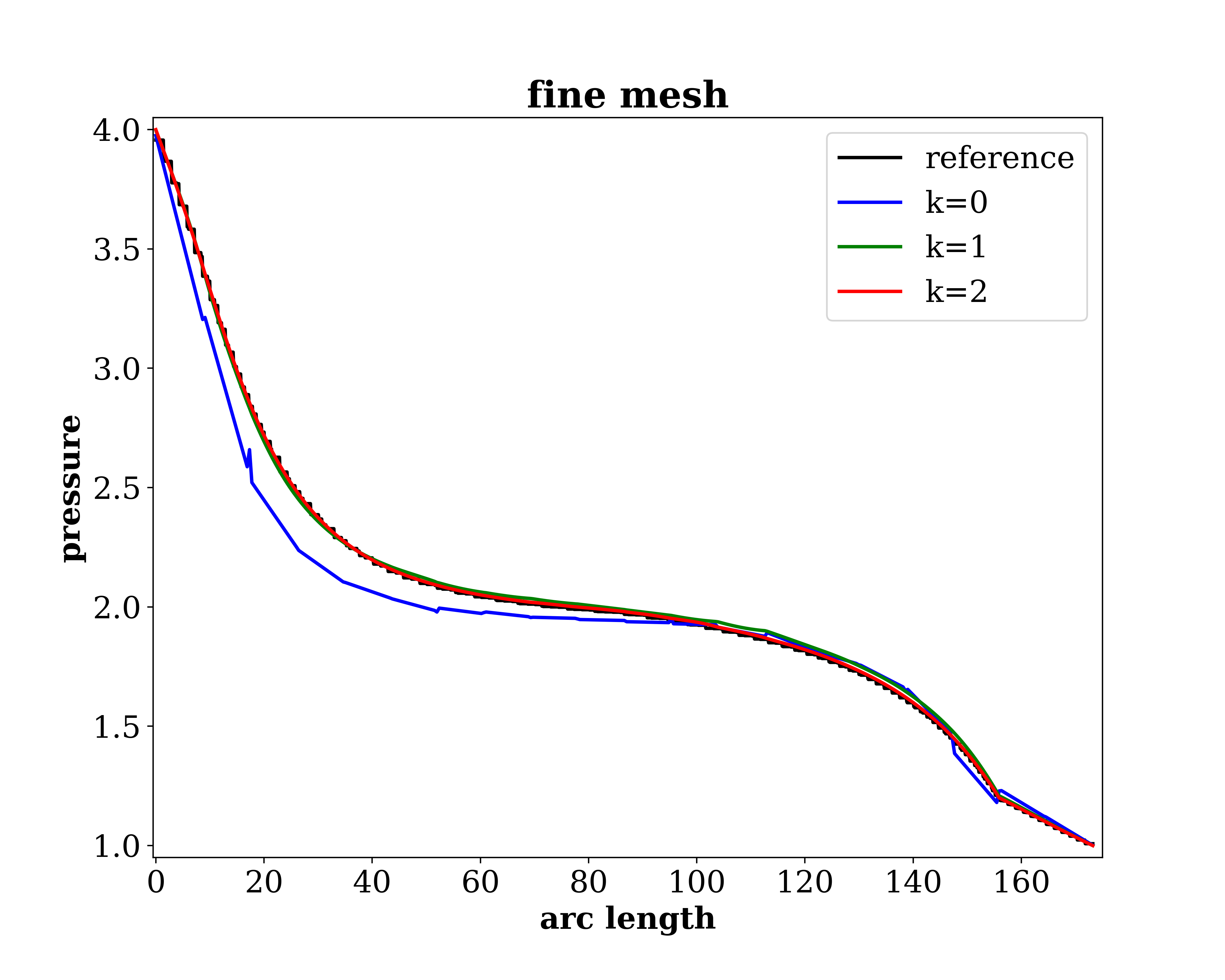
Figure 15. Example 4. Pressure along line $(0,0,0)--(100,100,100)$. Here reference data is the result from the USTUTT-MPFA scheme in [49] on a mesh with roughly 1 million matrix elements.

Example 5: Network with Small Features in 3D

This is the third benchmark case proposed in [49], in which small geometric features exist. The domain is the box $\Omega=(0,1)\times(0,2.25)\times(0,1)$, containing 8 planer conductive fractures; see Figure 16.

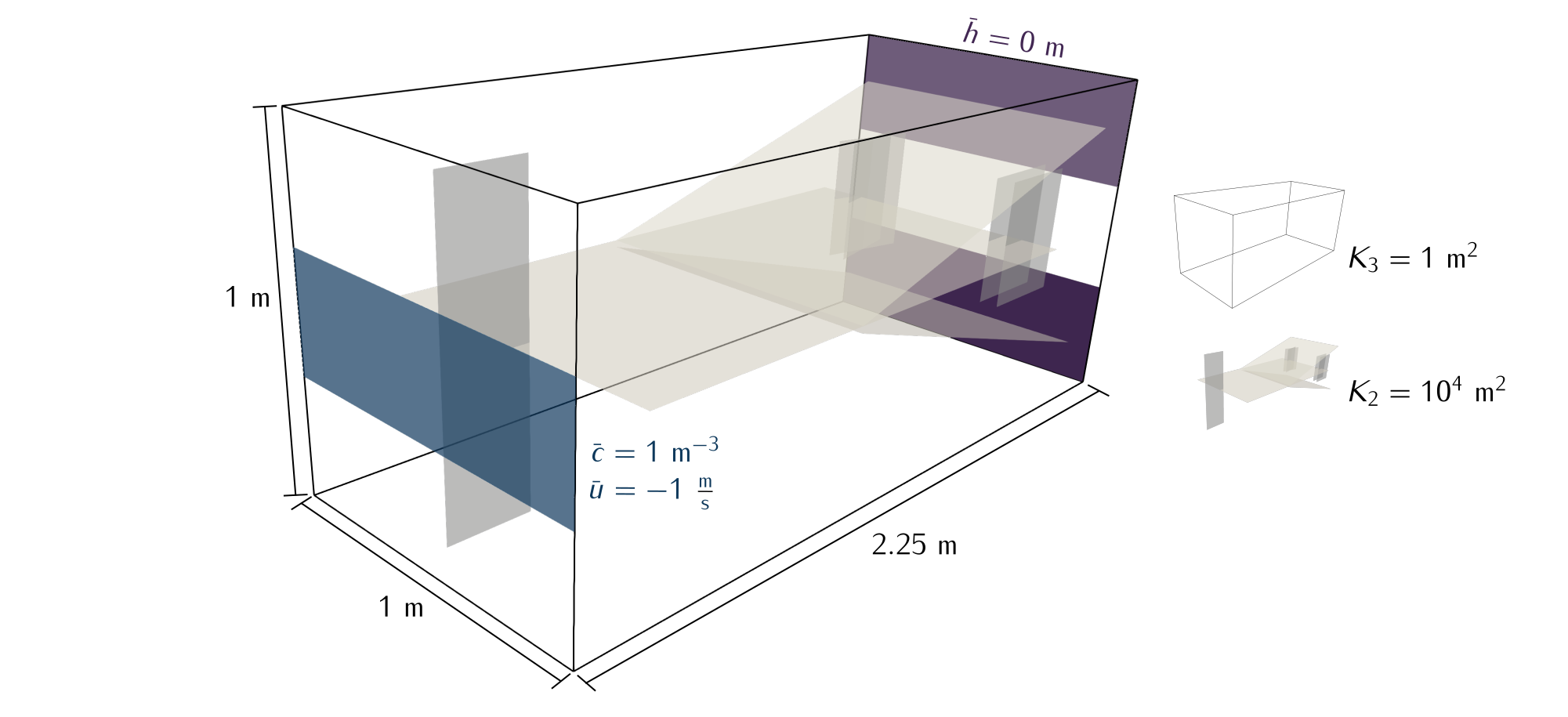
Figure 16. Example 5: Conceptual model and geometrical description of the domain.

Homogeneous Dirichlet boundary condition is imposed on the outlet boundary

$$\partial\Omega_{out}:=\{(x,y,z):0<x<1,y=2.25,z<1/3orz>2/3\},$$

inflow boundary condition $\hbox{\boldmath$u$}\cdot\hbox{\boldmath$n$}=-1$ is imposed on the inlet boundary

$$\partial\Omega_{in}:=\{(x,y,z):0<x<1,y=0,1/3<z<2/3\},$$

and no-flow boundary condition is imposed on the remaining boundaries. The permeability in the matrix is $\mathbb{K}_{m}=1$, and that in the fracture is $k_{c}=10^{4}$. Fracture thickness is $\epsilon=0.01$. The locations of these 8 fractures can be found in the git repository https://git.iws.uni-stuttgart.de/benchmarks/fracture-flow-3d where a sample gmsh geometric file was also provided. This problem is very challenging due to the small intersections among the fractures exist. The reported works in [49] showed large discrepancies among the 16 participating methods.

Here we run simulations for the scheme (4) with $k=0,1,2$ on two meshes: a fitted mesh with about 148k tetrahedral cells obtained from the above mentioned gmsh file with maximal mesh size $h\approx 0.074$ and minimal mesh size $h\approx 0.01$, and an unfitted mesh with about 132k tetrahedral cells obtained from local mesh refinements of a coarse uniform mesh near the fractures with maximal mesh size $h\approx 0.26$ and minimal mesh size $h\approx 0.026$. The penalty parameters for polynomial degree $k=0,1,2$ on these two meshes are shown in Table 2 below, where the characteristic length $L=2.25$.

	fitted mesh		unfitted mesh
$k$	$C_{c}$	$s_{c}$	$C_{c}$	$s_{c}$
0	5	2	2.5	2
1	0.7	3	0.7	3
2	3.5	3	0.7	3

Table 2. Example 5. Choice of the penalty parameters for different polynomial degree and meshes.

We first show the pressure contours along the plane $z=0.7$ which intersects with 6 fractures in Figure 17, from which we observe large variations among the results on the two meshes, especially for $y\geq 1$ where the fractures near the outlet starts to interact with the flow. This observation is in line with the findings in [49] where significant difference among participating methods were reported for the pressure distribution along the center line $(0.5,1.1,0)-(0.5,1.1,1.0)$, suggesting that the small features of the fracture network geometry may be not adequately resolved on these meshes. We also plot the pressure distribution along this center line in Figure 18, where the shaded region depicts the area between the 10th and the 90th percentile of the published results in [49] on similar meshes about $150k$ cells. It is observed from this figure that our results on both meshes are within the range of the published results in [49], and that the results on the fitted mesh may be more accurate as it is closer to the reference solution from USTUTT-MPFA on a mesh with roughly 1 million cells.

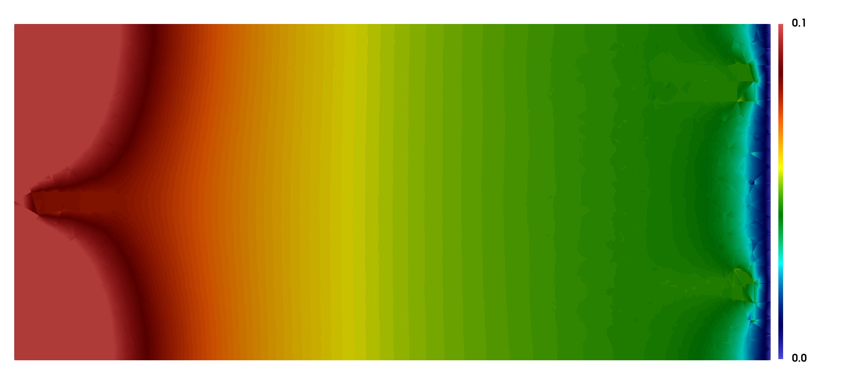
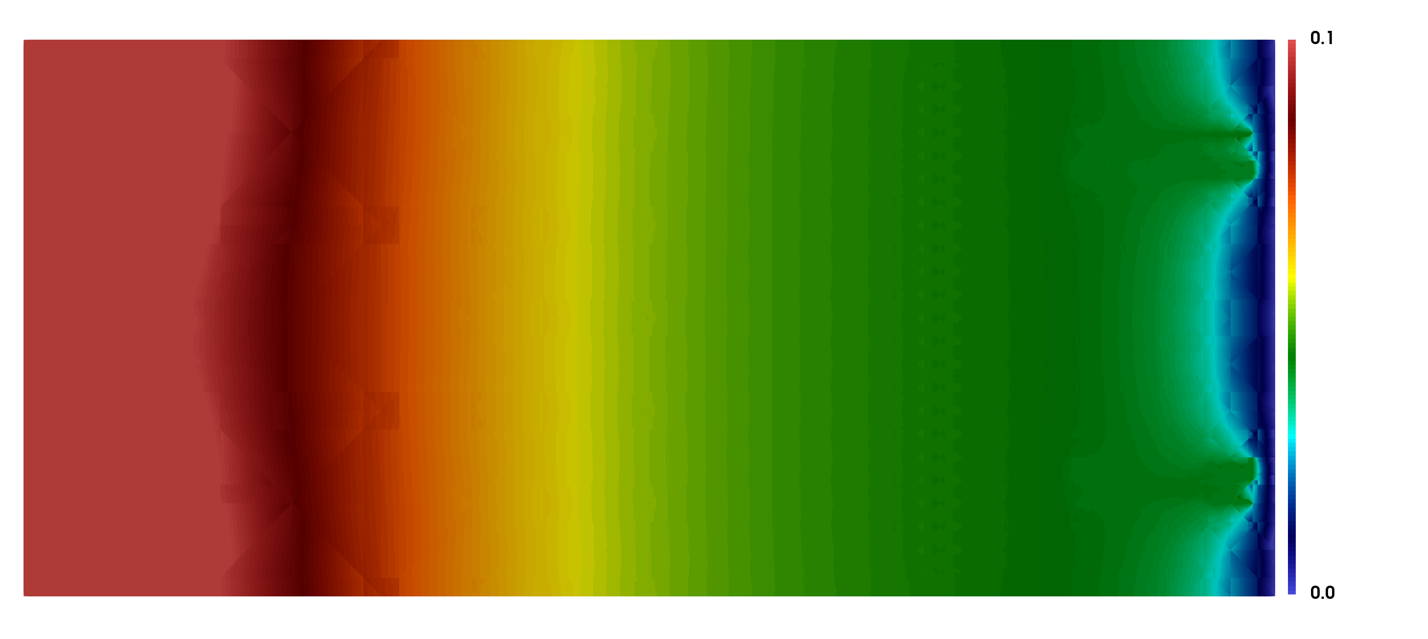
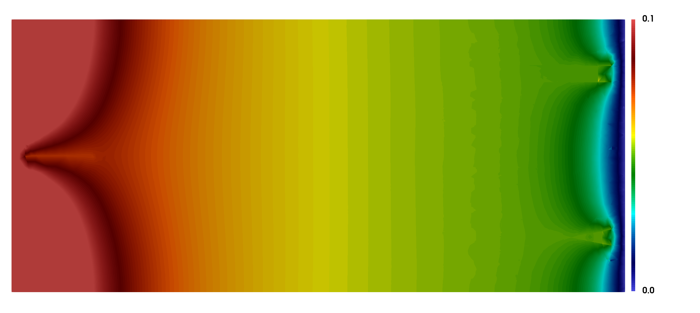
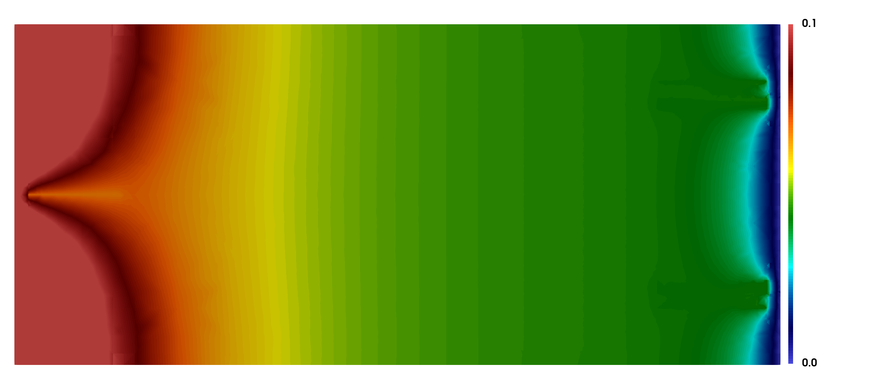
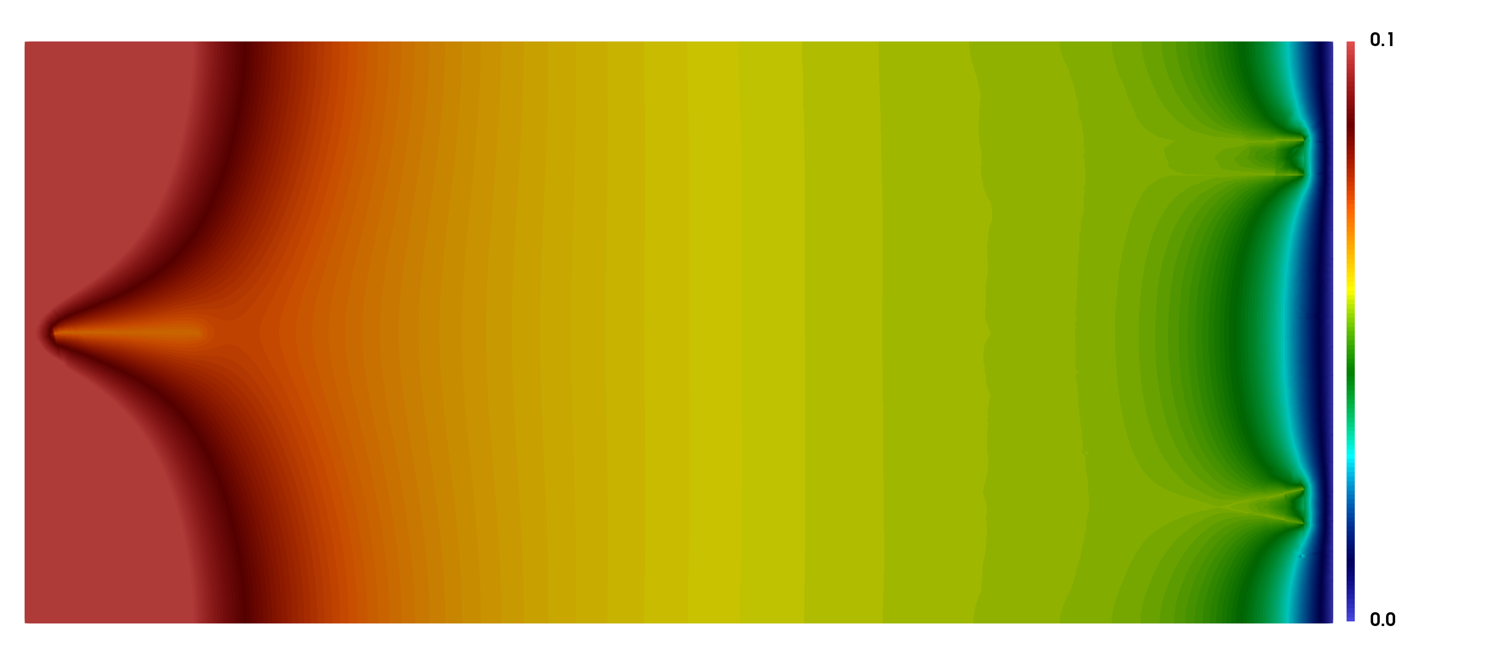
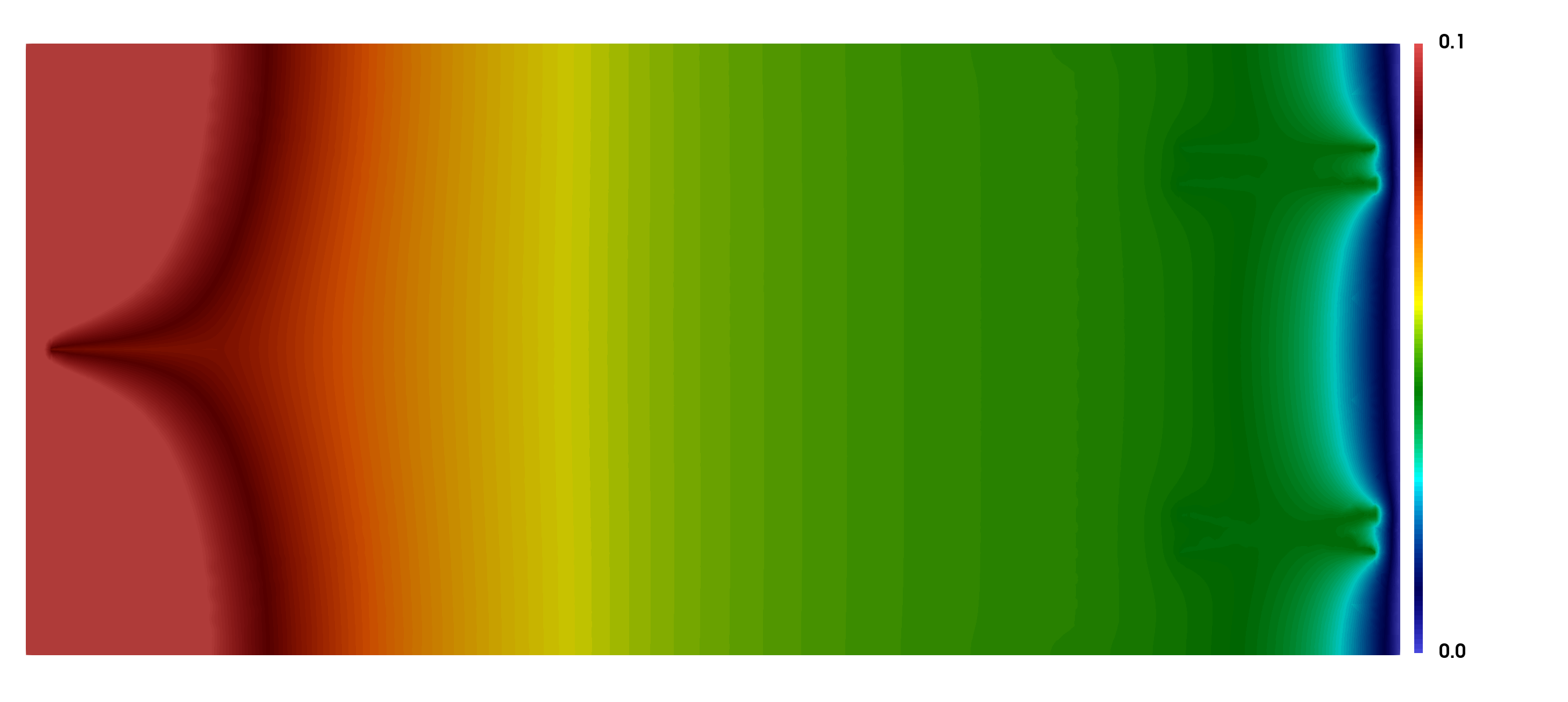
Figure 17. Example 5. Pressure contour on the plane $z=0.7$ for $k=0$ (top), $k=1$ (middle), and $k=2$ (bottom). Left: fitted mesh (1̃48k cells). Right: unfitted mesh (1̃32k cells).

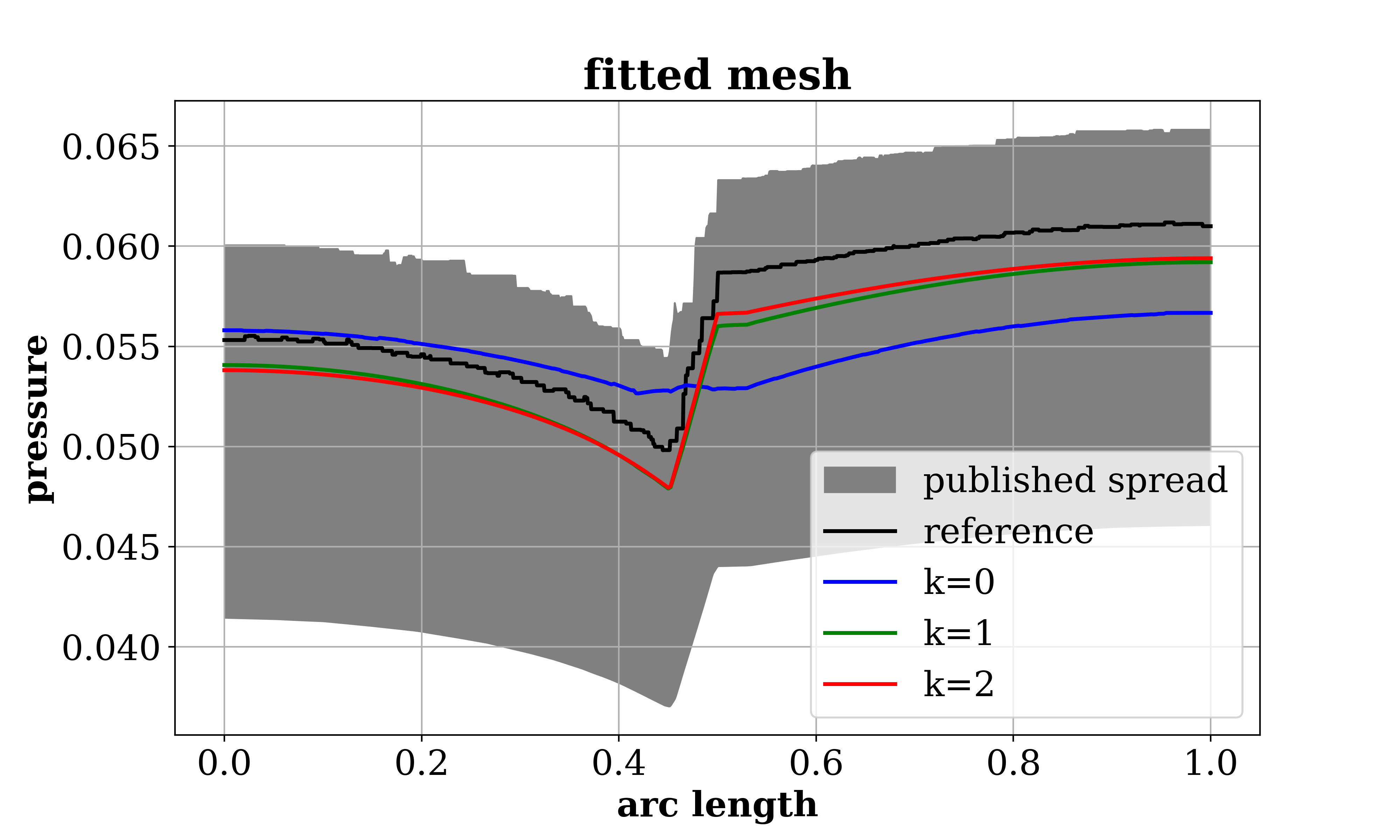
Figure 18. Example 5. Pressure along line $(0.5,1.1,0)--(0.5,1.1,1.0)$. Here reference data is the result from the USTUTT-MPFA scheme in [49] on a mesh with roughly 1 million matrix elements. The shaded region depicts the area between the 10th and the 90th percentile of the published results in [49] on similar meshes with about $150k$ cells.

Example 6: Field Case in 3D

In our final numerical example, we consider a similar setting as the last benchmark case proposed in [49]. The geometry is based on a postprocessed outcrop from the island of Algerøyna, outside Bergen, Norway, which contains 52 fracture. The simulation domain is the box $\Omega=(-500,350)\times(100,1500)\times(-100,500)$. The fracture geometry is depicted in Figure 19. Homogeneous Dirichlet boundary condition is imposed on the outlet boundary

$$\partial\Omega_{out}:=\underbrace{\{-500\}\times(100,400)\times(-100,100)}_{\partial\Omega_{out,0}}\;\cup\;\underbrace{\{350\}\times(100,400)\times(-100,100)}_{\partial\Omega_{out,1}}$$

uniform unit inflow $\hbox{\boldmath$u$}\cdot\hbox{\boldmath$n$}=1$ is imposed on the inlet boundary

$$\partial\Omega_{in}:=\underbrace{\{-500\}\times(1200,1500)\times(300,500)}_{\partial\Omega_{in,0}}\;\cup\;\underbrace{(-500,-200)\times\{1500\}\times(300,500)}_{\partial\Omega_{in,1}}.$$

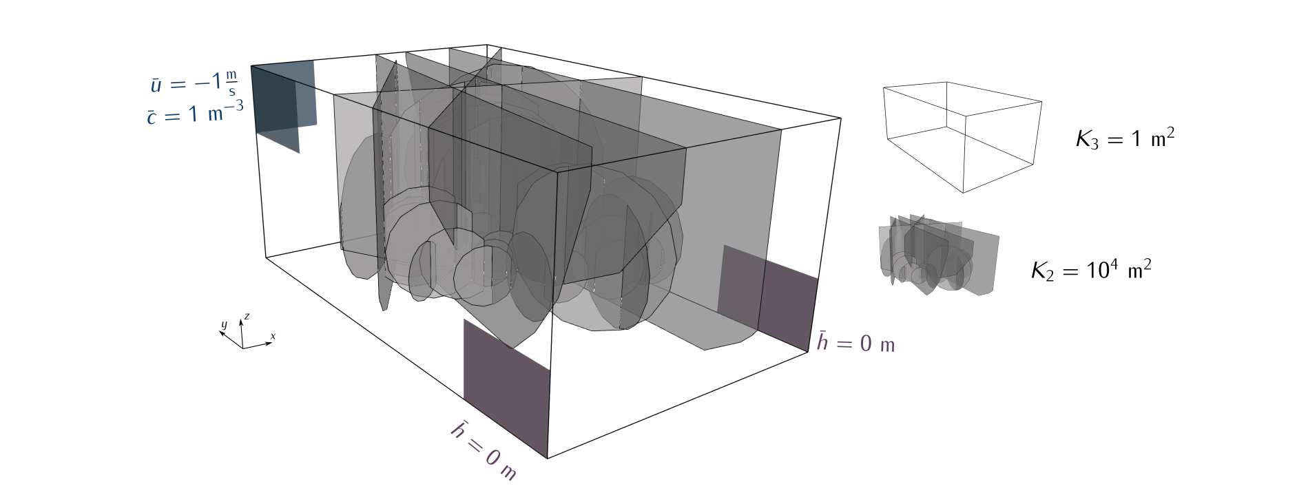
Figure 19. Example 6. Conceptual model and geometrical description of the domain.

Matrix permeability is $\mathbb{K}_{m}=1$, and fracture thickness is $\epsilon=10^{-2}$. Similar to Example 3 in 2D, we consider three subcases: (a) all conductive fractures with permeability $k_{c}=10^{4}$, (b) all blocking fractures with permeability $k_{b}=10^{-4}m^{2}$, and (c) 2 blocking fractures with $k_{b}=10^{-4}$ and 50 conductive fractures with $k_{c}=10^{4}$. Location of the blocking/conductive fractures for case (c) are marked in red/blue in the right panel of Figure 20.

We perform the method (4) on two unfitted meshes; see Figure 20 for the fine mesh. The coarse mesh contains $~{}27k$ tetrahedral cells which is obtained by performing two steps of local mesh refinement around the fractured cells of a uniform background mesh with $h\approx 200$. And the fine mesh contains $~{}210k$ cells with $~{}57.6k$ fractured cells which spits to $47.8$ conductive fractured cells and $9.8k$ blocking fractured cells for case (c), which is a further uniform refinement of that coarse mesh. As in the previous examples, we take polynomial degree $k=0,1,2$. For the penalty parameters, we take $C_{b}=1$, $s_{b}=2$, $C_{c}=1$ and the scaling power $s_{c}=3$ for $k=1$ and $k=2$, and $s_{c}=1$ for $k=0$. Moreover, for the case $k=0$ the default choice of stabilization (4k) is too strong which leads to almost constant (zero) pressure approximations for case (a). Here we further reduce the stabilization for $k=0$ by a factor of $L=1400$.

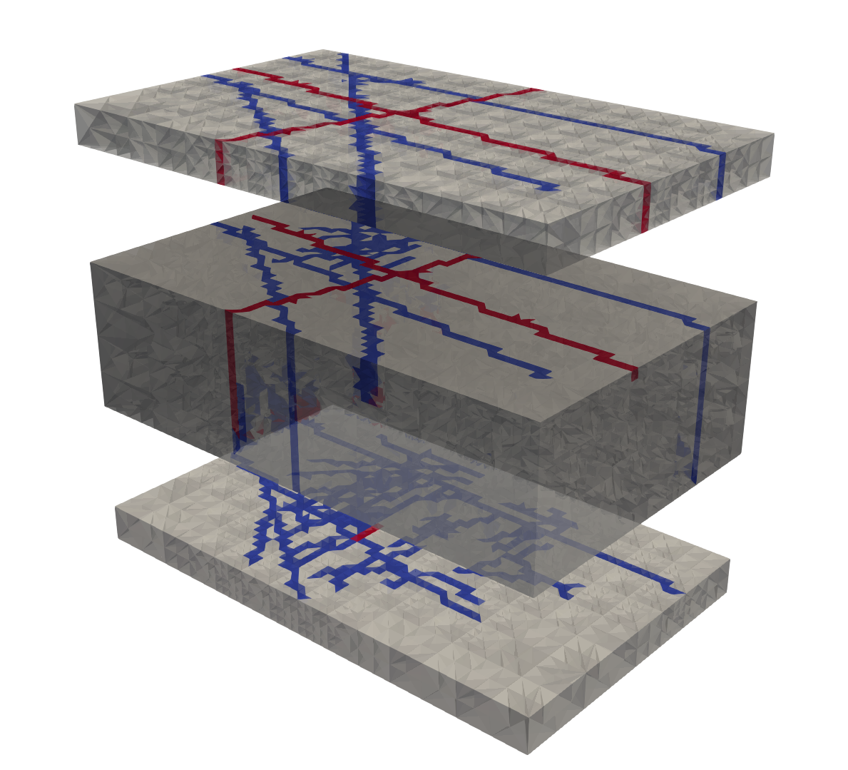
Figure 20. Example 6. Blocking (red) and conductive (blue) fractured cells on the fine mesh with 216816 cells for case (c). Here the mesh is translated in the $z$-direction for $z<100$ and $z>400$ for better data visualization.

The pressure along the two diagonal lines $(-500,100,-100)$–$(350,1500,500)$ and $(350,100,-100)$–$(-500,1500,500)$ are shown in Figures 21-23 for all three cases, where for case (a) the shaded region depicts the area between the 10th and the 90th percentile of the published results in [49] on fitted meshes with about $260k$ cells. It is observed that all methods produce qualitatively similar results for each case, even on the coarse mesh. And our results for case (a) is consistent with the published results in [49].

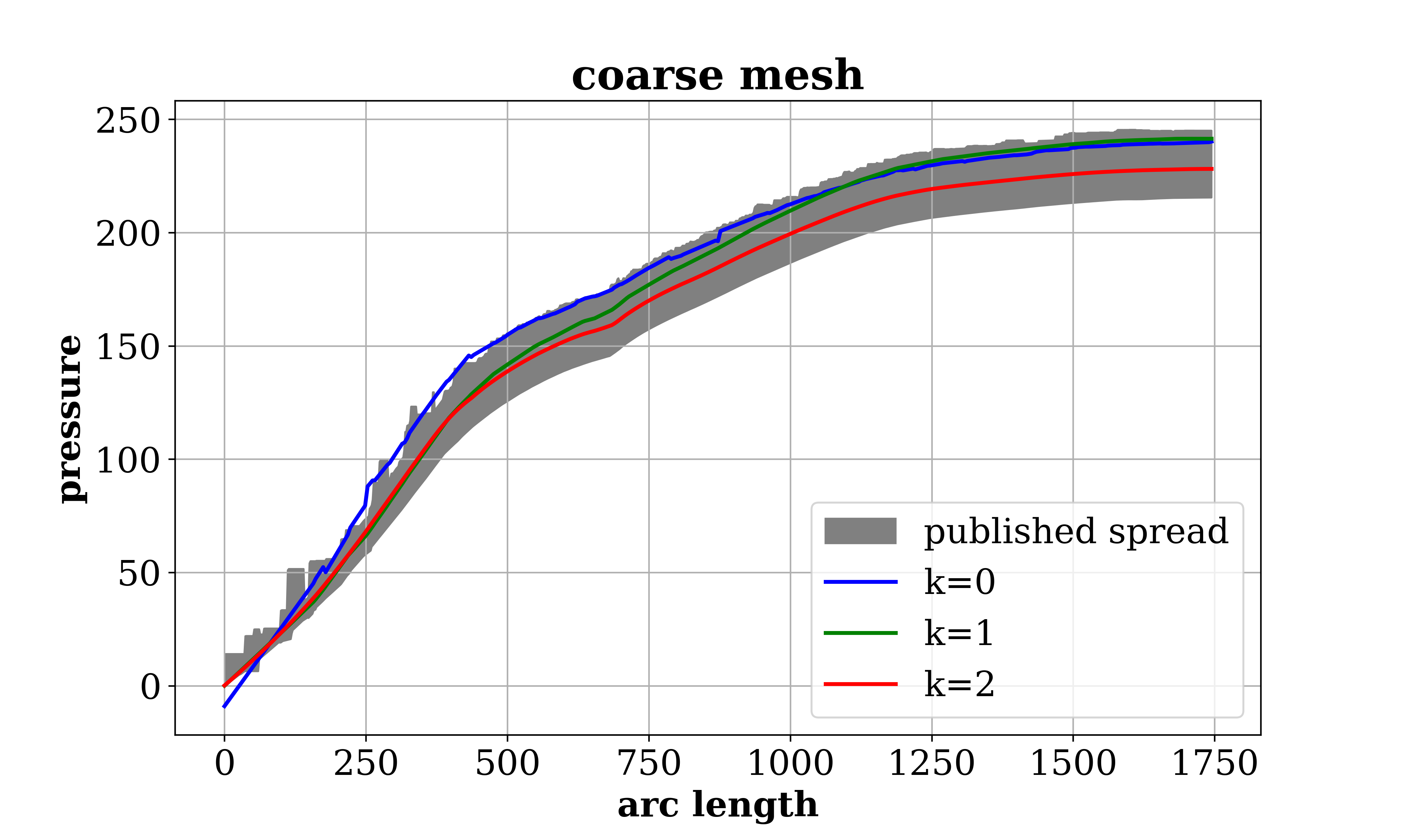
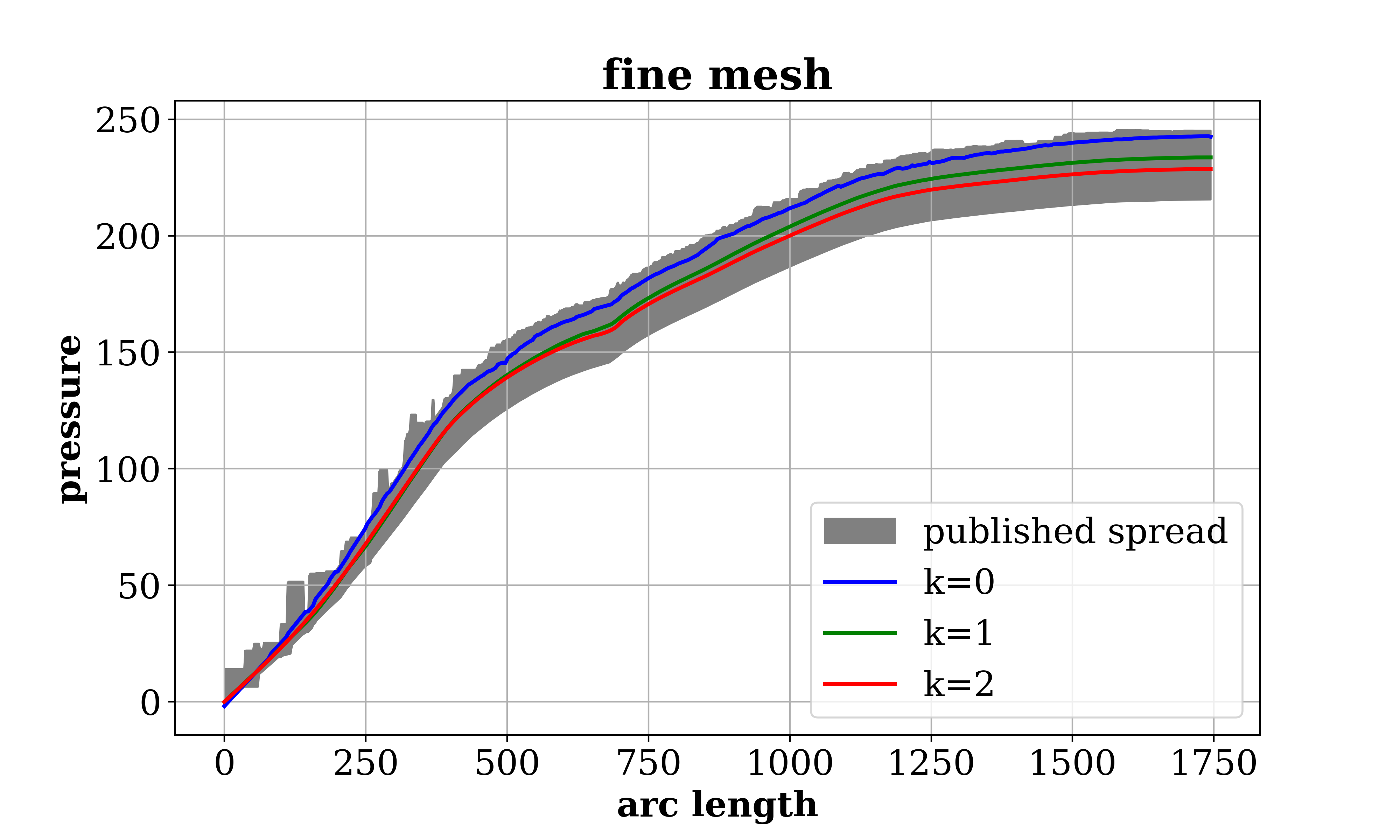
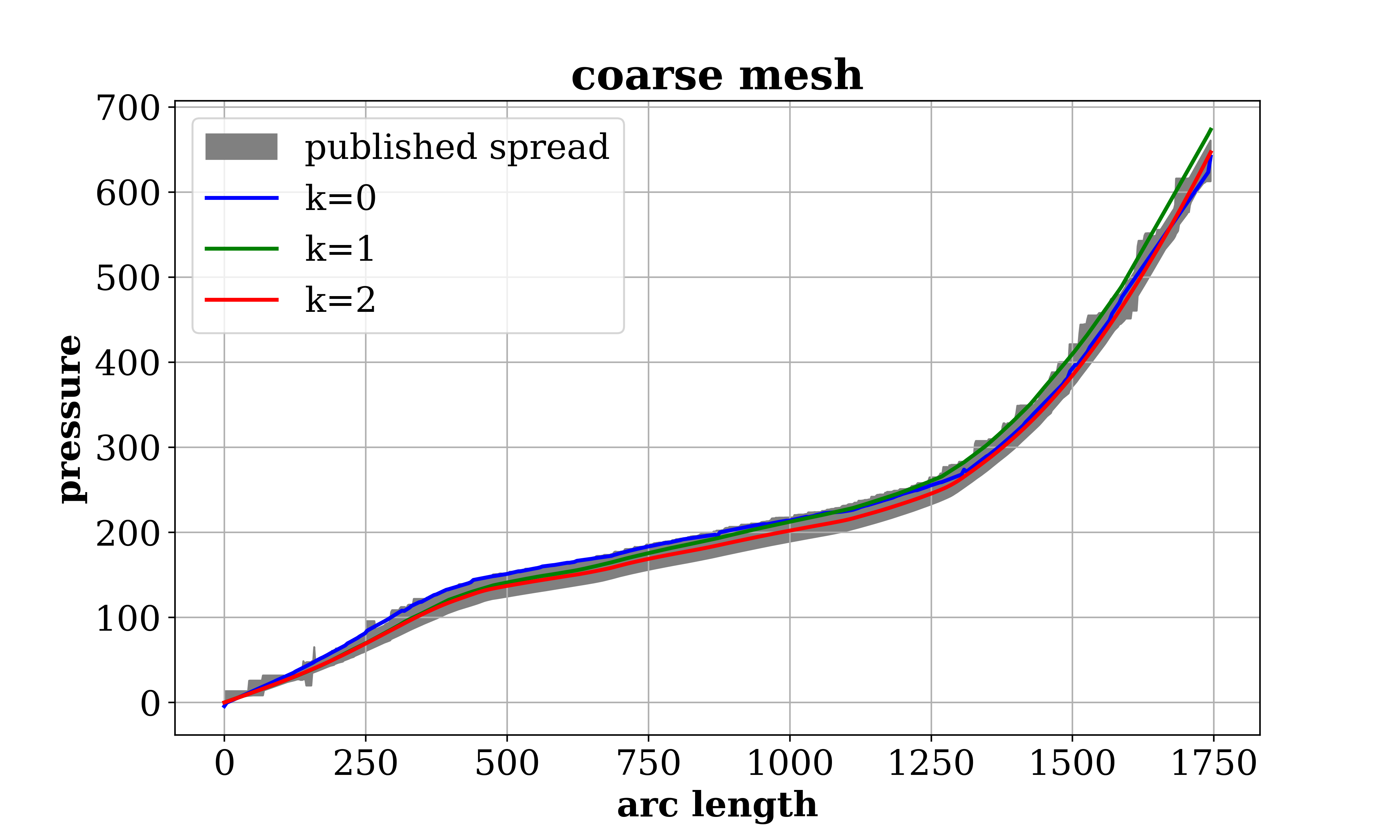
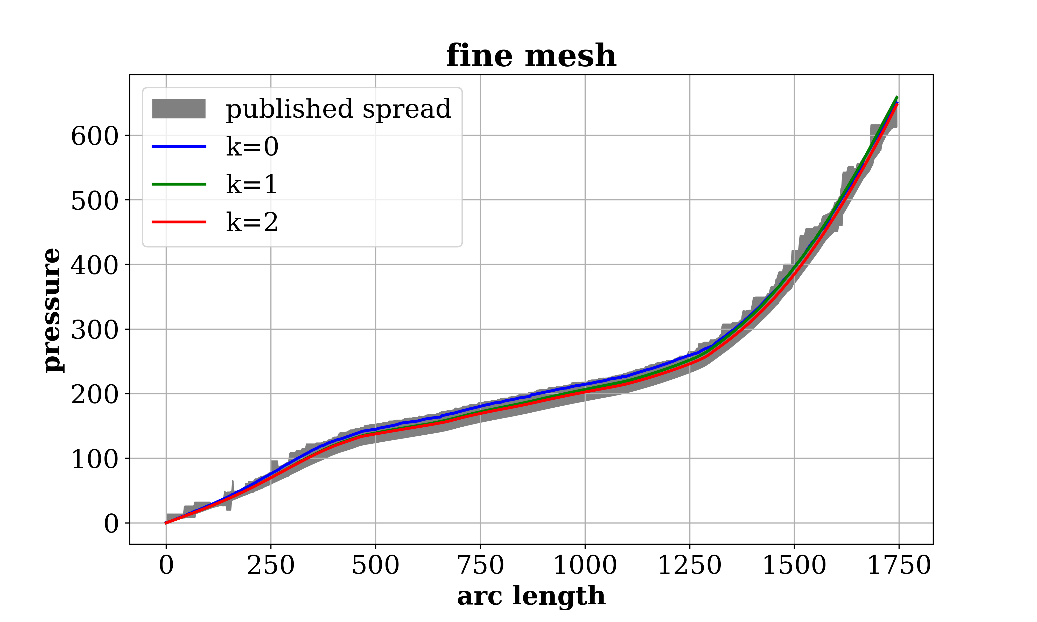
Figure 21. Example 6: Case (a). Pressure along line $(-500,100,-100)$–$(350,1500,500)$ (top) and line $(350,100,-100)$–$(-500,1500,500)$ (bottom). The shaded region depicts the area between the 10th and the 90th percentile of the published results in [49] on fitted meshes with about $260k$ cells.

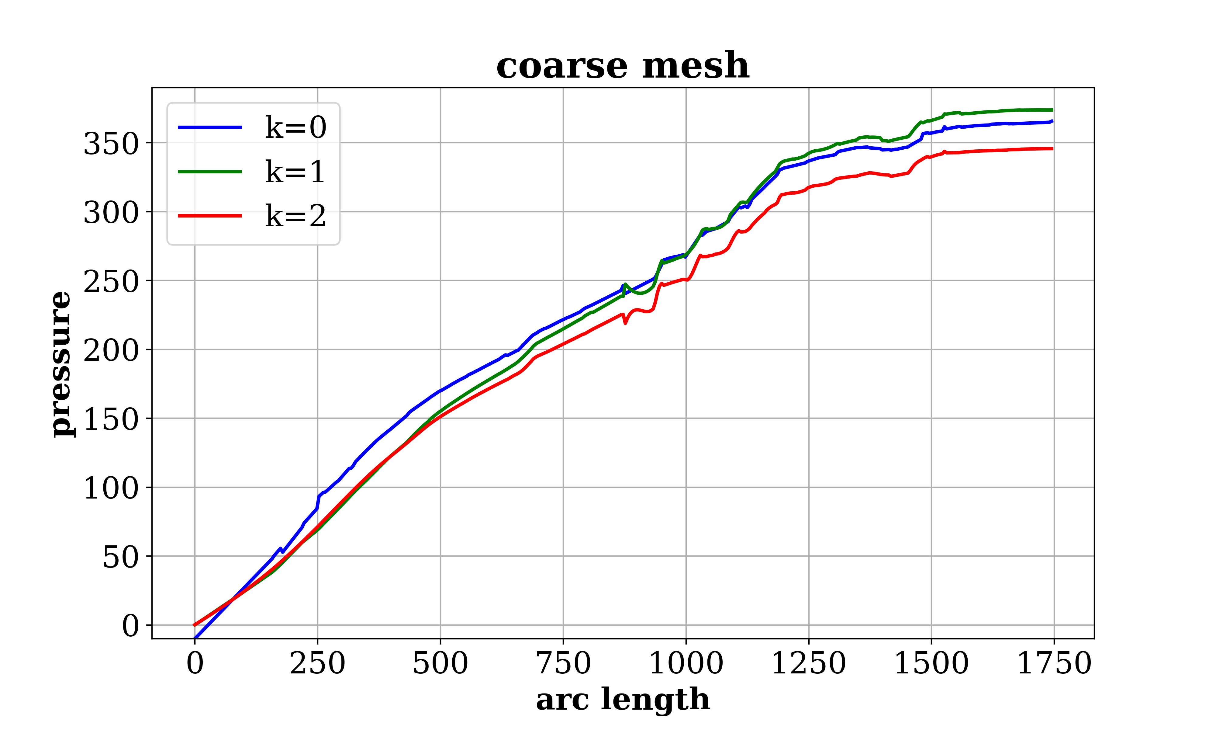
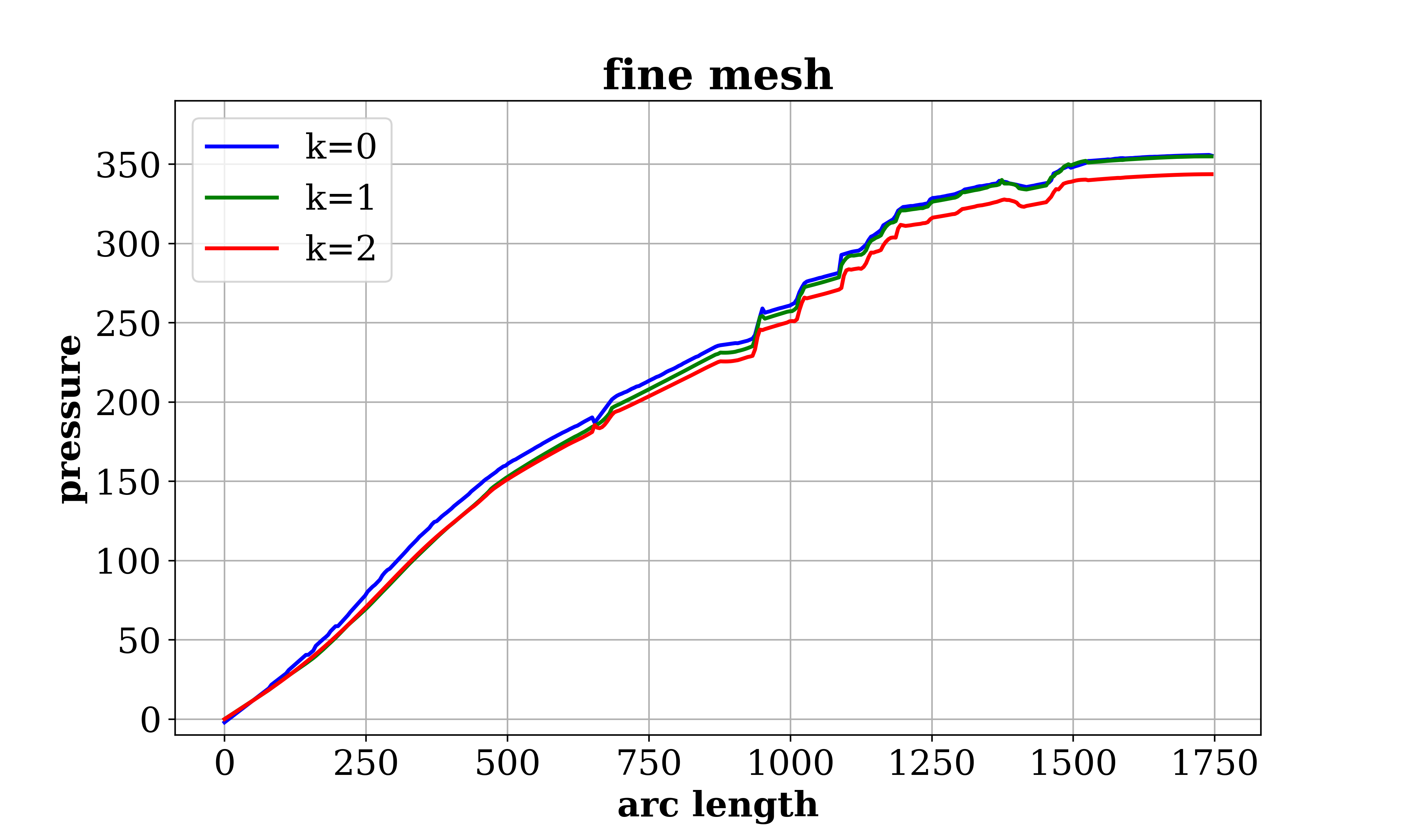
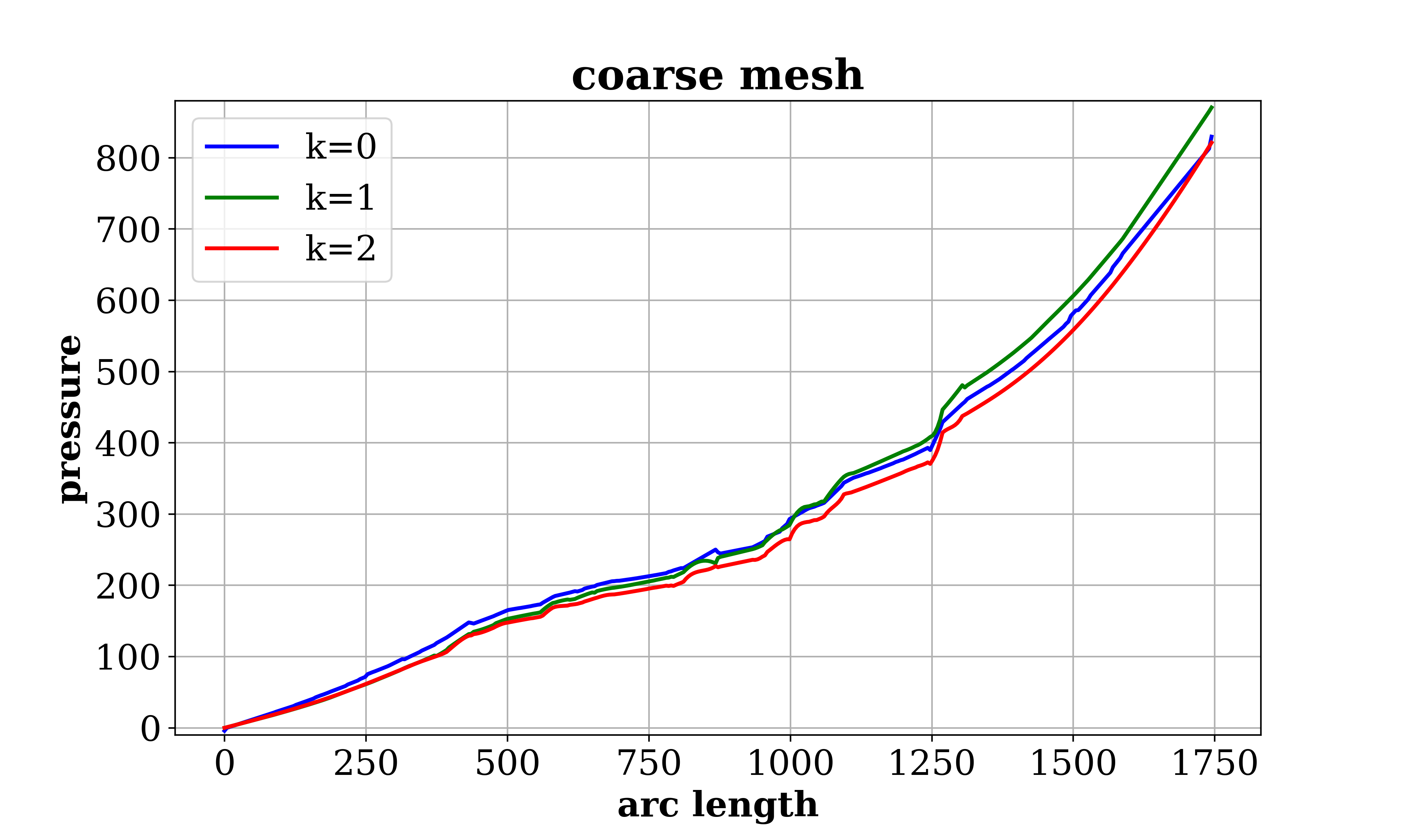
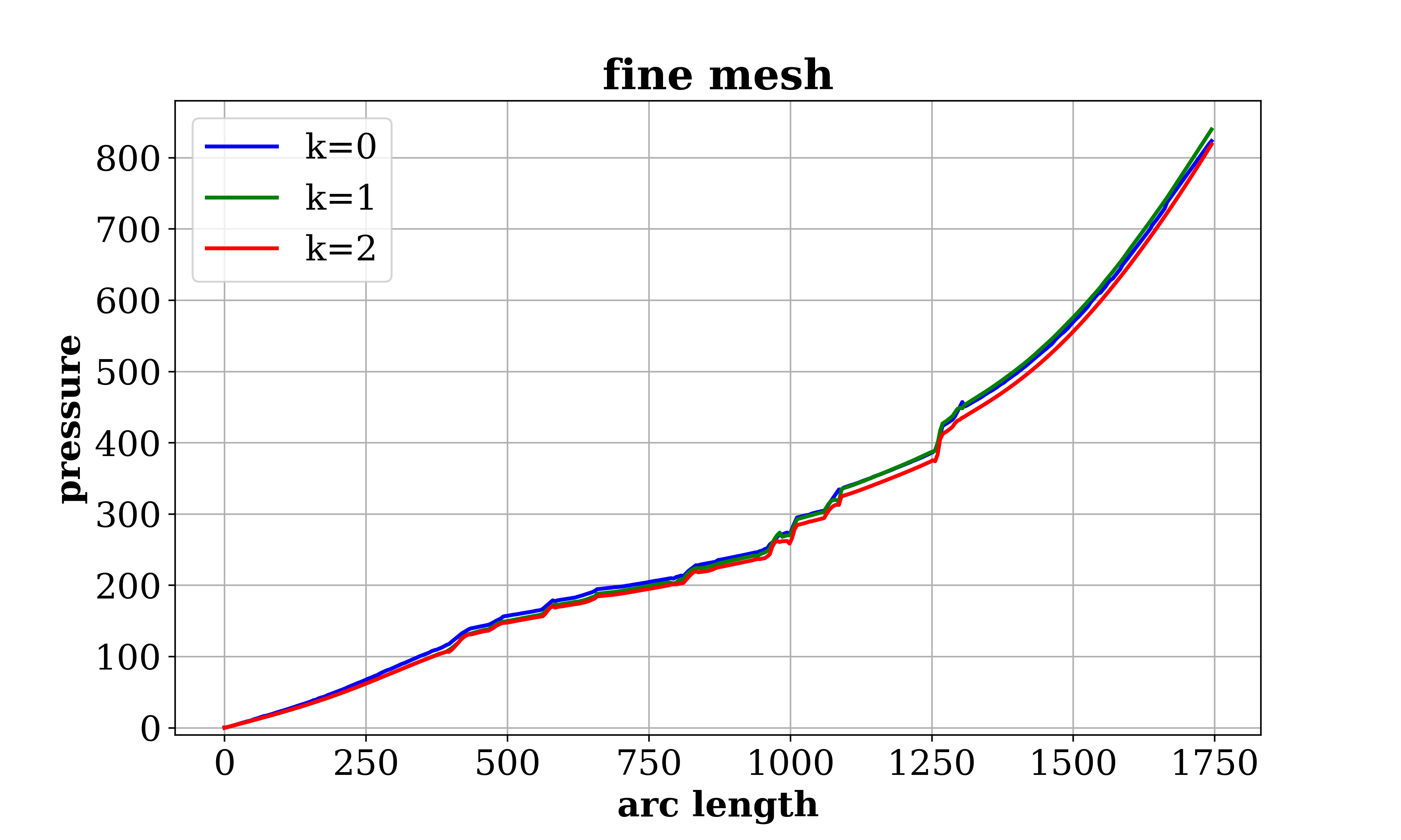
Figure 22. Example 6: Case (b). Pressure along line $(-500,100,-100)$–$(350,1500,500)$ (top) and line $(350,100,-100)$–$(-500,1500,500)$ (bottom).

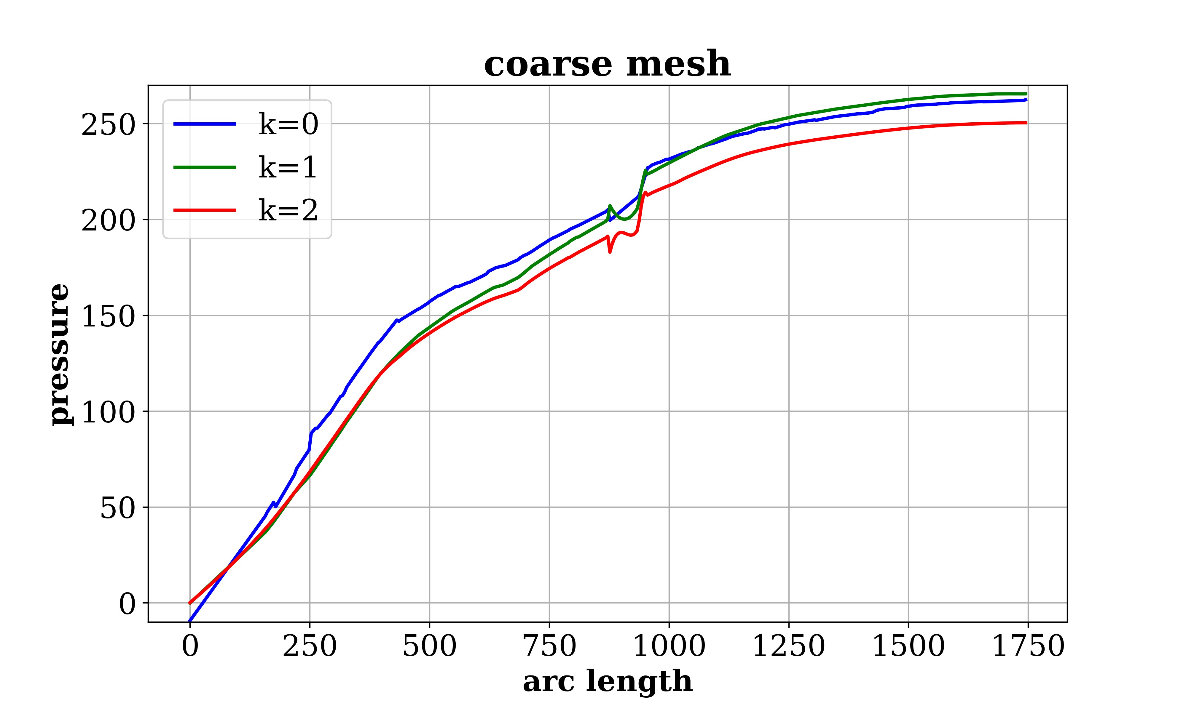
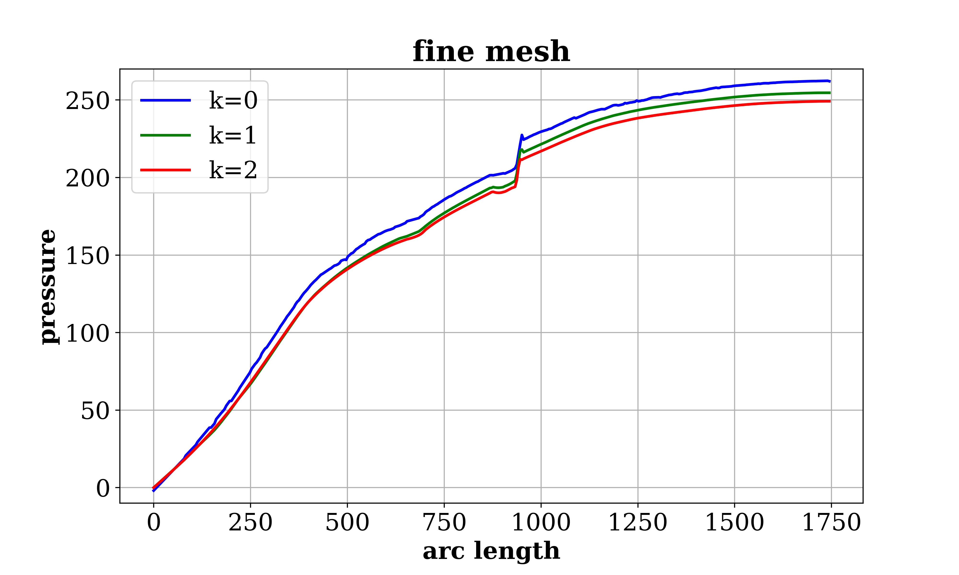
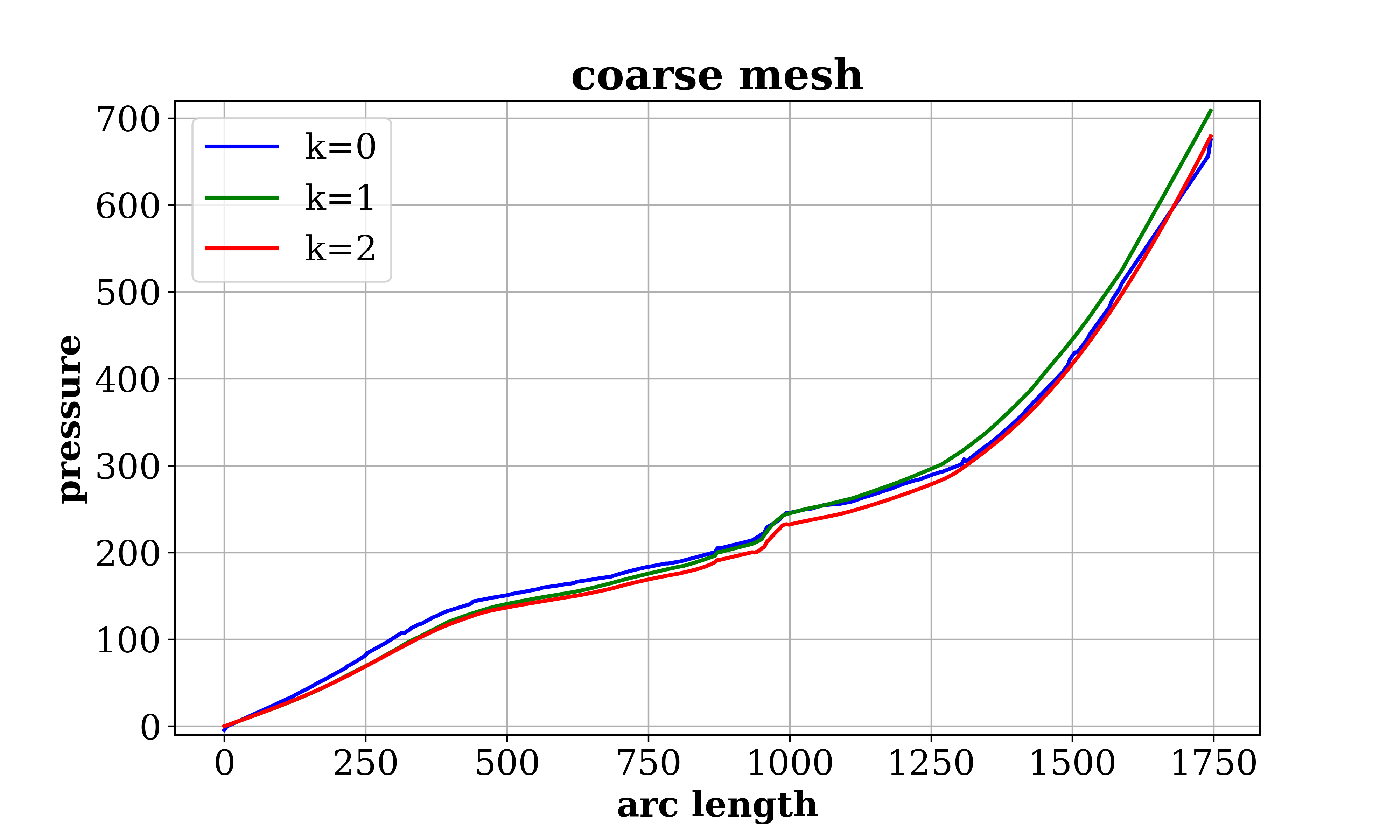
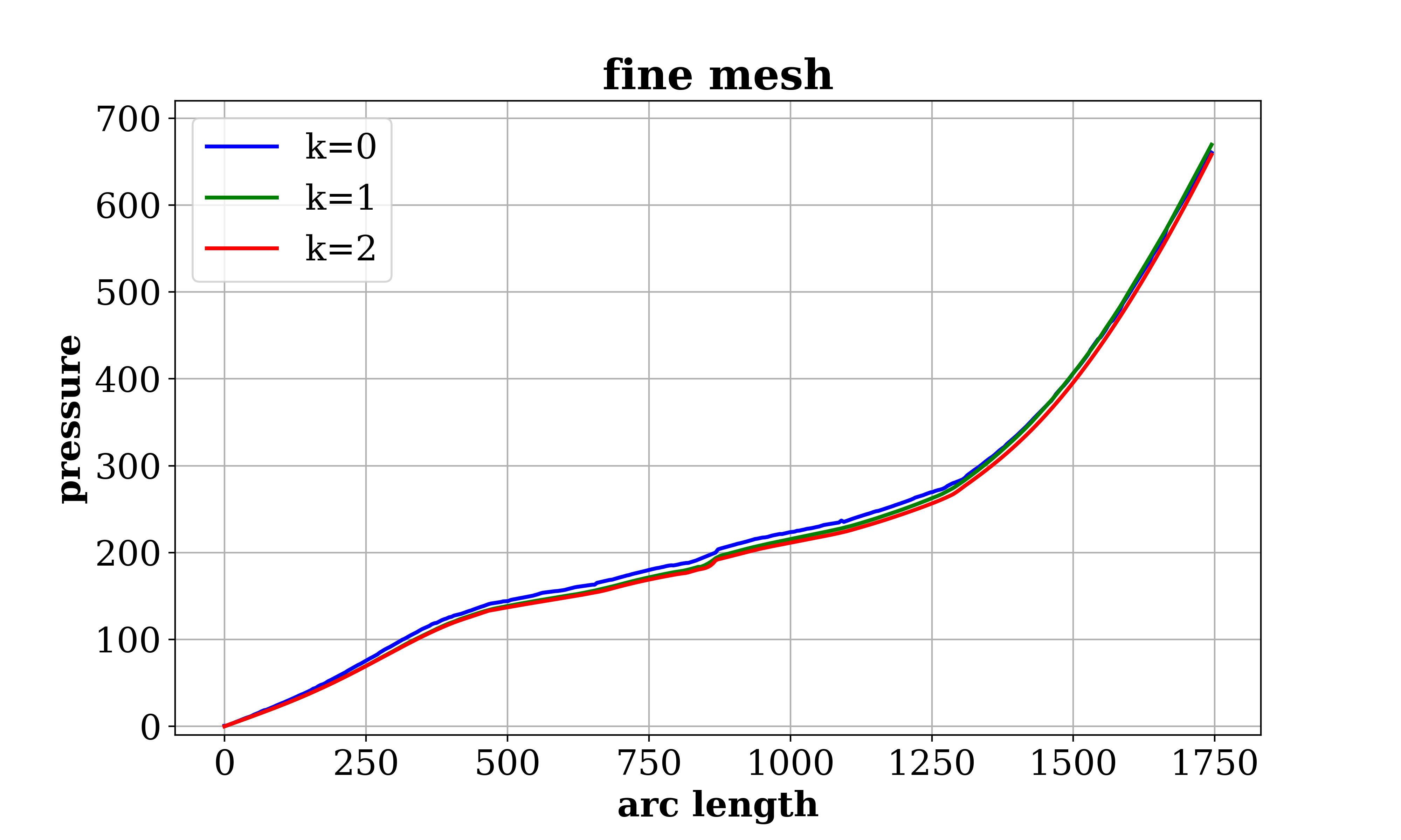
Figure 23. Example 6: Case (c). Pressure along line $(-500,100,-100)$–$(350,1500,500)$ (top) and line $(350,100,-100)$–$(-500,1500,500)$ (bottom).

We now plot the pressure profile on the fine mesh for $k=2$ for the three cases in Figure 24. These contour plots are similar to the 2D results where the effects of conductive and blocking fractures are completely different as expected.

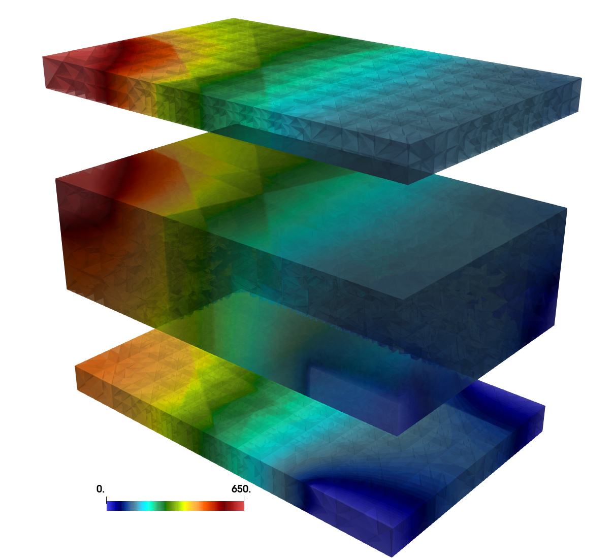
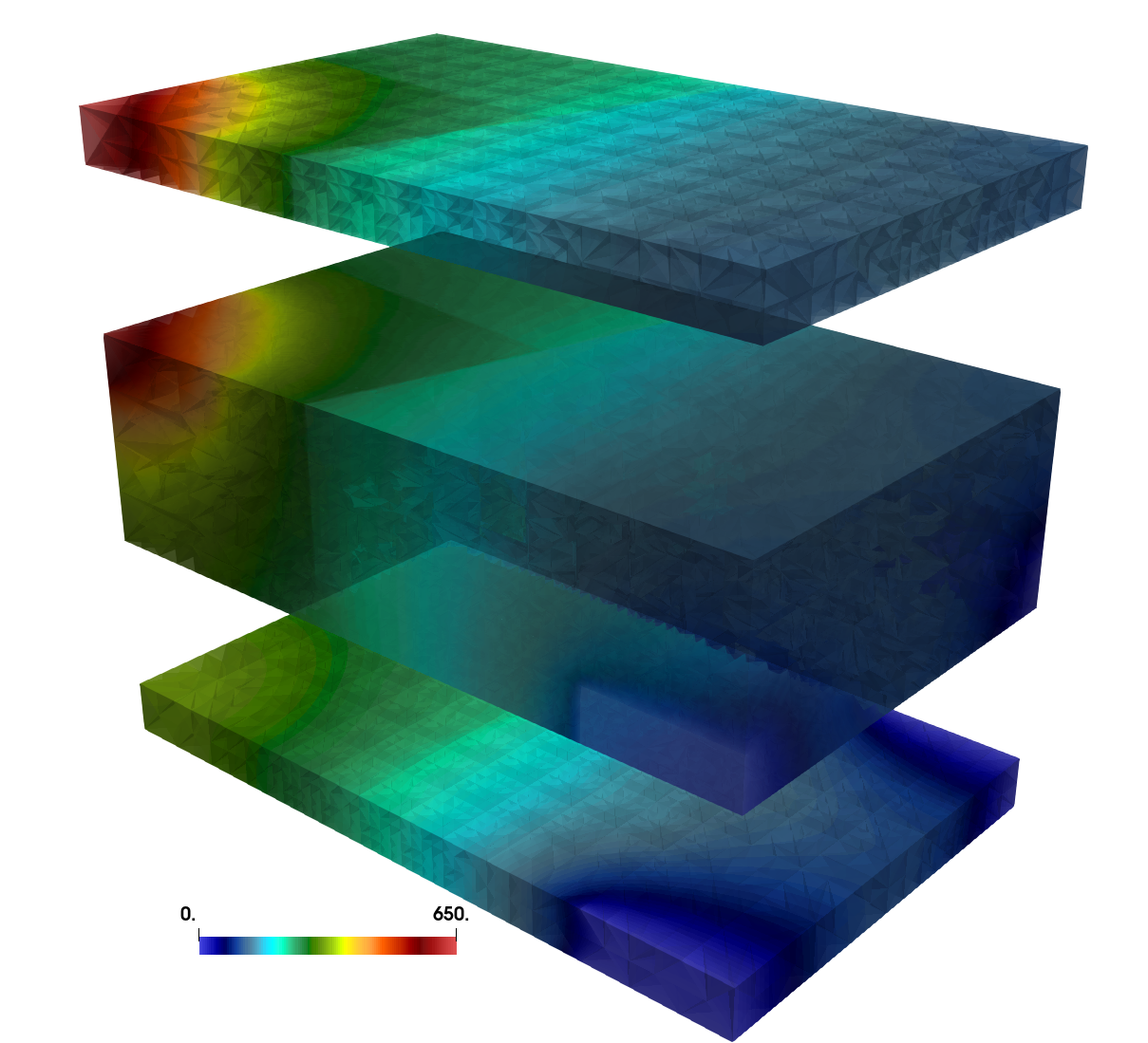
Figure 24. Example 6. Pressure contour for $k=2$ on the fine mesh. Left: case (a). Middle: case (b). Right: case (c).

Let us finally briefly comment on the computational cost on the fine mesh where the major bottleneck is the global linear system solve. Here we use NGsolve’s built-in parallel sparse Cholesky factorization to solve this global SPD linear system on a 64-core server with two Two AMD EPYC 7532 processors which has 256G memory. For $k=0$, there are $439k$ global DOFs, and the linear system solver takes 30G memory and 4 seconds wall clock time; for $k=1$, there are $1.32$ million global DOFs, and the linear system solver takes 50G memory and 48 seconds wall clock time; for $k=2$, there are $2.64$ million global DOFs, and the linear system solver takes 100G memory and 285 seconds wall clock time. More efficient solver like multigrid may significantly reduce the memory consumption and overall solver time. We will investigate this issue in our future work.

4. Conclusion

We presented a novel HDG scheme on unfitted meshes for fractured porous media flow with both blocking and conductive fractures based on the RDFM using Dirac-$\delta$ functions approach to handle the fractures. Well-posedness of the method is established. Our scheme is relatively easy to implement comparing with most existing fractured porous media flow solvers in the literature that can simultanuously handel blocking and conductive fractures. In fact, we simply modify a regular porous media flow HDG solver by including two surface integrals related to the blocking and conductive fractures which are represented as (multi-)level set functions, and properly adjust the penalty parameters in the numerical flux on those fractured cells. No lower dimensional fracture modeling is needed in our approach. Besides the ease of using unfitted meshes in our scheme, we also maintain local conservation as typical of DG methodologies. Moreover, the resulting linear system can be solved efficiently via static condensation, which leads to a global coupled SPD linear system, and higher order pressure postprocessing is also available. The proposed HDG scheme is extensively tested against various benchmark examples in two- and three-dimensions. Satisfactory results are observed even when both blocking and conductive fractures co-exist in the computational domain.

Our future work includes the detailed study of the stabilization function on the performance of the scheme, and their variable-order and hybrid-mixed variants. We will also investigate robust preconditioning techniques for the global SPD linear system, and extend our solver to multiphase fractured porous media flows.

References

- [1] Z. Xu, Z. Huang, and Y. Yang, “The hybrid-dimensional Darcy’s law: a novel discrete fracture model for fracture and barrier networks on non-conforming meshes,” 2021. Submitted.
- [2] G. I. Barenblatt, I. P. Zheltov, and I. N. Kochina, “Basic concepts in the theory of seepage of homogeneous liquids in fissured rocks [strata],” Journal of applied mathematics and mechanics, vol. 24, no. 5, pp. 1286–1303, 1960.
- [3] J. E. Warren and P. J. Root, “The behavior of naturally fractured reservoirs,” Society of Petroleum Engineers Journal, vol. 3, pp. 245–255, 1963.
- [4] S. Geiger, M. Dentz, and A. I. Neuweiler, “Novel multi-rate dual-porosity model for improved simulation of fractured and multiporosity reservoirs,” SPE J., 0, vol. 4, pp. 670–684, 2013.
- [5] K. Ghorayeb and A. Firoozabadi, “Numerical study of natural convection and diffusion in fractured porous media,” Spe Journal, vol. 5, pp. 12–20, 2000.
- [6] J. Noorishad and M. Mehran, “An upstream finite element method for solution of transient transport equation in fractured porous media,” Water Resources Research, vol. 18, no. 3, pp. 588–596, 1982.
- [7] R. G. Baca, R. C. Arnett, and D. W. Langford, “Modelling fluid flow in fractured‐porous rock masses by finite‐element techniques,” International Journal for Numerical Methods in Fluids, vol. 4, no. 4, pp. 337–348, 1984.
- [8] J. G. Kim and M. D. Deo, Comparison of the performance of a discrete fracture multiphase model with those using conventional methods. In SPE Reservoir Simulation Symposium. Society of Petroleum Engineers, 1999, January.
- [9] J. G. Kim and M. D. Deo, “Finite element, discrete‐fracture model for multiphase flow in porous media,” AIChE Journal, vol. 46, no. 6, pp. 1120–1130, 2000.
- [10] M. Karimi-Fard and A. Firoozabadi, “Numerical simulation of water injection in 2D fractured media using discrete-fracture model,” Society of Petroleum Engineers, 2001. In SPE annual technical conference and exhibition.
- [11] S. Geiger-Boschung, S. K. Matth”ai, J. Niessner, and R. Helmig, “Black-oil simulations for three-component, three-phase flow in fractured porous media,” SPE journal, vol. 14, no. 02, pp. 338–354, 2009.
- [12] N. Zhang, J. Yao, Z. Huang, and Y. Wang, “Accurate multiscale finite element method for numerical simulation of two-phase flow in fractured media using discrete-fracture model,” Journal of Computational Physics, vol. 242, pp. 420–438, 2013.
- [13] L. Li and S. H. Lee, “Efficient field-scale simulation of black oil in a naturally fractured reservoir through discrete fracture networks and homogenized media,” SPE Reservoir Evaluation & Engineering, vol. 11, no. 04, pp. 750–758, 2008.
- [14] A. Moinfar, “Development of an efficient embedded discrete fracture model for 3D compositional reservoir simulation in fractured reservoirs,” 2013. Ph.D. Thesis, University of Texas, Austin.
- [15] X. Yan, Z. Huang, J. Yao, Y. Li, and D. Fan, “An efficient embedded discrete fracture model based on mimetic finite difference method,” Journal of Petroleum Science and Engineering, vol. 145, pp. 11–21, 2016.
- [16] M. Tene, S. Bosma, M. Al Kobaisi, and H. Hajibeygi, “Projection-based embedded discrete fracture model (pEDFM),” Advances in Water Resources, vol. 105, pp. 205–216, 2017.
- [17] J. Jiang and R. M. Younis, “An improved projection-based embedded discrete fracture model (pEDFM) for multiphase flow in fractured reservoirs,” Advances in water resources, vol. 109, pp. 267–289, 2017.
- [18] M. HosseiniMehr, M. Cusini, C. Vuik, and H. Hajibeygi, “Algebraic dynamic multilevel method for embedded discrete fracture model (F-ADM),” Journal of Computational Physics, vol. 373, pp. 324–345, 2018.
- [19] J. Xu, B. Sun, and B. Chen, “A hybrid embedded discrete fracture model for simulating tight porous media with complex fracture systems,” Journal of Petroleum Science and Engineering, vol. 174, pp. 131–143, 2019.
- [20] C. Alboin, J. Jaffré, J. Roberts, and C. Serres, “Domain decomposition for flow in porous media with fractures,” in Domain Decomposition Methods in Sciences and Engineering (M. C. C. H. Lai, P. E. Bjorstad, and O. Widlund, eds.), pp. 365–373, Domain Decomposition Press, Bergen, Norway: vol. 53, 1999.
- [21] C. Alboin, J. Jaffré, J. E. Roberts, X. Wang, and C. Serres, “Domain decomposition for some transmission problems in flow in porous media,” in Numerical Treatment of Multiphase Flows in Porous Media, pp. 22–34, Berlin: Springer, Heidelberg, 2000.
- [22] A. Hansbo and P. Hansbo, “An unfitted finite element method, based on nitsche’s method, for elliptic interface problems,” Computer methods in applied mechanics and engineering, vol. 191, no. 47-48, pp. 5537–5552, 2002.
- [23] L. H. Odsæter, T. Kvamsdal, and M. G. Larson, “A simple embedded discrete fracture–matrix model for a coupled flow and transport problem in porous media,” Computer Methods in Applied Mechanics and Engineering, vol. 343, pp. 572–601, 2019.
- [24] A. Fumagalli and A. Scotti, “An efficient XFEM approximation of Darcy flows in arbitrarily fractured porous media,” Oil & Gas Science and Technology–Revue d’IFP Energies nouvelles, vol. 69, no. 4, pp. 555–564, 2014.
- [25] H. Huang, T. A. Long, J. Wan, and W. P. Brown, “On the use of enriched finite element method to model subsurface features in porous media flow problems,” Computational Geosciences, vol. 15, no. 4, pp. 721–736, 2011.
- [26] N. Schwenck, “An XFEM-based model for fluid flow in fractured porous media,” 2015. Ph.D. Thesis, Universität Stuttgart.
- [27] S. Salimzadeh and N. Khalili, “Fully coupled XFEM model for flow and deformation in fractured porous media with explicit fracture flow,” International Journal of Geomechanics, vol. 16, no. 4, p. 04015091, 2015.
- [28] B. Flemisch, A. Fumagalli, and A. Scotti, “A review of the XFEM-based approximation of flow in fractured porous media,” in Advances in Discretization Methods, pp. 47–76, Springer, Cham., 2016.
- [29] M. Köppel, V. Martin, J. Jaffré, and J. E. Roberts, “A Lagrange multiplier method for a discrete fracture model for flow in porous media,” Computational Geosciences, vol. 23, no. 2, pp. 239–253, 2019.
- [30] M. Köppel, V. Martin, and J. E. Roberts, “A stabilized Lagrange multiplier finite-element method for flow in porous media with fractures,” GEM-International Journal on Geomathematics, vol. 10, 2019. Article number: 7 (2019).
- [31] P. Schädle, P. Zulian, D. Vogler, S. R. Bhopalam, M. G. Nestola, A. Ebigbo, R. Krause, and M. O. Saar, “3D non-conforming mesh model for flow in fractured porous media using Lagrange multipliers,” Computers and Geosciences, vol. 132, pp. 42–55, 2019.
- [32] V. Martin, J. Jaffré, and J. E. Roberts, “Modeling fractures and barriers as interfaces for flow in porous media,” SIAM Journal on Scientific Computing, vol. 26, no. 5, pp. 1667–1691, 2005.
- [33] P. Angot, F. Boyer, and F. Hubert, “Asymptotic and numerical modelling of flows in fractured porous media,” ESAIM: Mathematical Modelling and Numerical Analysis, vol. 43, no. 2, pp. 239–275, 2009.
- [34] W. Boon, J. Nordbotten, and I. Yotov, “Robust discretization of flow in fractured porous media,” SIAM Journal on Numerical Analysis, vol. 56, pp. 2203–2233, 2018.
- [35] T. Kadeethum, H. Nick, S. Lee, and F. Ballarin, “Flow in porous media with low dimensional fractures by employing enriched galerkin method,” Advances in Water Resources, vol. 142, p. 103620, 2020.
- [36] J. Jiang and R. M. Younis, “An improved projection-based embedded discrete fracture model (pEDFM) for multiphase flow in fractured reservoirs,” Advances in water resources, vol. 109, pp. 267–289, 2017.
- [37] B. Flemisch, I. Berre, W. Boon, A. Fumagalli, N. Schwenck, A. Scotti, I. Stefansson, and A. Tatomir, “Benchmarks for single-phase flow in fractured porous media,” Advances in Water Resources, vol. 111, pp. 239–258, 2018.
- [38] E. Burman, P. Hansbo, M. G. Larson, and K. Larsson, “Cut finite elements for convection in fractured domains,” Computers and Fluids, vol. 179, pp. 726–734, 2019.
- [39] Z. Xu and Y. Yang, “The hybrid dimensional representation of permeability tensor: A reinterpretation of the discrete fracture model and its extension on nonconforming meshes,” Journal of Computational Physics, vol. 415, p. 109523, 2020.
- [40] W. Feng, H. Guo, Z. Xu, and Y. Yang, “Conservative numerical methods for the reinterpreted discrete fracture model on non-conforming meshes and their applications in contaminant transportation in fractured porous media,” Advances in Water Resources, vol. 153, p. 103951(16), 2021.
- [41] G. Fu and Y. Yang, “A hybrid-mixed finite element method for single-phase Darcy flow in fractured porous media,” Advances in Water Resources, vol. 161, p. 104129, 2022.
- [42] B. Cockburn, J. Gopalakrishnan, and R. Lazarov, “Unified hybridization of discontinuous Galerkin, mixed and continuous Galerkin methods for second order elliptic problems,” SIAM Journal on Numerical Analysis, vol. 47, pp. 1319–1365, 2009.
- [43] B. Cockburn, J. Gopalakrishnan, and F.-J. Sayas, “A projection-based error analysis of HDG methods,” Mathematics of Computation, vol. 79, pp. 1351–1367, 2010.
- [44] R. Yang, Y. Xing, and Y. Yang, “Sign-preserving high order well-balanced discontinuous Galerkin methods for the shallow water equations with friction terms,” Journal of Computational Physics, vol. 44, p. 110543(23), 2021.
- [45] B. Cockburn, O. Dubois, J. Gopalakrishnan, and S. Tan, “Multigrid for an HDG method,” IMA J. Numer. Anal., vol. 34, no. 4, pp. 1386–1425, 2014.
- [46] G. Fu, “Uniform auxiliary space preconditioning for HDG methods for elliptic operators with a parameter dependent low order term,” SIAM J. Sci. Comput., vol. 43, no. 6, pp. A3912–A3937, 2021.
- [47] J. Schöberl, “C++11 Implementation of Finite Elements in NGSolve,” 2014. ASC Report 30/2014, Institute for Analysis and Scientific Computing, Vienna University of Technology.
- [48] C. Lehrenfeld, F. Heimann, J. Preuß, and H. von Wahl, “ngsxfem: Add-on to ngsolve for geometrically unfitted finite element discretizations,” Journal of Open Source Software, vol. 6, no. 64, p. 3237, 2021.
- [49] I. Berre, W. Boon, B. Flemisch, A. Fumagalli, D. Gläser, E. Keilegavlen, A. Scotti, I. Stefansson, A. Tatomir, K. Brenner, S. Burbulla, P. Devloo, O. Duran, M. Favino, J. Hennicker, I.-H. Lee, K. Lipnikov, R. Masson, K. Mosthaf, M. C. Nestola, C.-F. Ni, K. Nikitin, P. Schädle, D. Svyatskiy, R. Yanbarisov, and P. Zulian, “Verification benchmarks for single-phase flow in three-dimensional fractured porous media,” Advances in Water Resources, vol. 147, p. 103759, 2021.