Semi-parametric generalized estimating equations for repeated measurements in cross-over designs

Abstract

A model for cross-over designs with repeated measures within each period was developed. It is obtained using an extension of generalized estimating equations that includes a parametric component to model treatment effects and a non-parametric component to model time and carry-over effects; the estimation approach for the non-parametric component is based on splines. A simulation study was carried out to explore the model properties. Thus, when there is a carry-over effect or a functional temporal effect, the proposed model presents better results than the standard models. Among the theoretical properties, the solution is found to be analogous to weighted least squares. Therefore, model diagnostics can be made adapting the results from a multiple regression. The proposed methodology was implemented in the data sets of the crossover experiments that motivated the approach of this work: systolic blood pressure and insulin in rabbits.

1 Introduction

In the context of crossover experimental designs, each experimental unit receives a sequence of treatments, and each treatment is applied over a period of time (Biabani et al., 2018). These designs are very useful in medical experimentation, since they require fewer experimental units to obtain the same results as cross-sectional studies. The disadvantage is given by the appearance of carry-over effects, which are defined as the residual effects that remain in the response of the individual and that are caused by the treatments applied in the previous periods (Madeyski and Kitchenham (2018) and Kitchenham et al. (2018)).

The most recent works on the analysis of crossover designs assume the non-existence of carry-over effects, due to the presence of a washout period between the successive applications of treatments (Curtin, 2017). This assumption is common in works based on classical generalized linear models (Li et al., 2018), Bayesian models (Oh et al., 2003) or generalized estimating equation (GEE) models (Curtin, 2017). However, in some crossover designs the length of the washout period is very short and does not guarantee the elimination of the residual effects of each of the treatments, such as the one presented in Jones and Kenward (2015, page 204). In this design, three treatments for blood pressure control are used and treatment C is a placebo. In this experiment, if there is a carry-over effect of the placebo, it is not cleaned in the washout period. The doctors tried to control the hypertension in patients, and so, treatments can be stopped for a very short time due to the characteristics of the disease.

Furthermore, in the design presented in Jones and Kenward (2015, pag 204), the systolic blood pressure is observed ten times within each period: 30 and 15 minutes before the application, and 15, 30, 45, 60, 75, 90 , 120 and 240 minutes after the application, as seen in the Table 1, which generates a repeated measurement for each application period. This type of design is known as a repeated measures crossover design (Dubois et al., 2011). Dubois et al. (2011), Diaz et al. (2013) and Forbes et al. (2015) used Gaussian linear mixed models to study cross-over repeated measures designs. However, those studies considered one observation per period by calculating the area under the curve, and they did not include the carry-over effects. Additionally, this modeling does not allow us to observe the temporal behavior of the response variable within the period, nor the presence of carry-over effects that fluctuate over time.

On the other hand, when the response variable of the crossover experiment shown by Kenward and Roger (2009) is analyzed, it is observed that it does not adequately fit a normal distribution. Since the response in this experiment is blood sugar levels, which are skewed and always positive, a gamma distribution seems more suitable for analysis. In both experiments, we have a response that can be assumed to be in the exponential family and the responses of the same experimental unit are correlated. Therefore, in this paper we propose an extension of the GEE with splines to model the effects of main interest in the design (treatments, period) with a parametric component and the temporary effects through smoothing splines.

This methodology makes it possible to unbiasedly isolate the temporal behavior of the carry-over effect from the period and treatment effects, which is demonstrated theoretically and through a simulation exercise. Subsequently, when applying the methodology in the blood pressure design, a significant carry-over effect of the placebo treatment is obtained, corroborating the importance of taking it into account in the analysis.

Sequence	Period 1	Period 2	Period 3
(1) ABC Ind 1 Ind 2	10 observations 10 observations	10 observations 10 observations	10 observations 10 observations
⋮	⋮	⋮	⋮
(6) CBA Ind 11 Ind 12	10 observations 10 observations	10 observations 10 observations	10 observations 10 observations

Table 1: Structure of the blood pressure crossover design, with three period, six sequences and ten measurements (that were taken -30, -15, 15, 30, 45, 60, 75, 90, 120 and 240 minutes from application) per period

This paper is structured as follows: In Section 2, the semiparametric model with GEE was described, and the estimation equations are derived. In section 3, asymptotic consistency and unbiasedness of estimators are established. In Section 4, a simulation study is carried out to display the advantages of the proposed model over those models often found in the literature and some diagnostics measures for its residuals. In Section 5, an application of to blood pressure data is performed out to illustrate the model properties and to carry out an overall analysis of this dataset. Finally, some conclusions are presented in Section 6.

2 Repeated measures cross-over design

A cross-over design entails five components (Jones and Kenward, 2015): i) sequences which are randomly assigned combinations of the applied treatments on the experimental units, ii) treatments, that are applied to each experimental unit as a part of a sequence in a given time, iii) periods, that represent the application lapse for the treatments which are part of a sequence, v) experimental units, which are the elements on which a treatment is applied.
In each sequence, there are $n_{l}$ experimental units, therefore the total number of experimental units is $n=\sum_{l=1}^{S}n_{l}$ Further, it is frequent that each period has the same length for all sequences, therefore, the number of observation periods equals the length of each sequence.
For the structure of cross-over designs, the carry-over effects constitute part of them. Vegas et al. (2016) defined the carry-over as a treatment’s effect persistence over those treatments applied later. That is, if a treatment is applied on a given period, then there exists the possibility of a residual or carry-over effect that persists in the following periods when other treatments are applied. When the carry-over effect of a treatment affects the one applied in the next period, it is known as a frist-order carry over effect.
In a cross-over design with $S$ sequences of length $P$, let $n_{ij}$ be the number of observations on the $i$-th experimental unit and $j$-th period, then $\boldsymbol{Y}_{ij}$ is a vector defined as:

$$\boldsymbol{Y}_{ij}=\left(Y_{ij1},\ldots,Y_{ijn_{ij}}\right)^{T}$$ (1)

Moreover, we define a vector $\boldsymbol{Y}_{i}$ vector contains every observation on the $i$-th experimental unit

$$\boldsymbol{Y}_{i}=\left(\boldsymbol{Y}_{i1},\ldots,\boldsymbol{Y}_{iP}\right)^{T}$$ (2)

and its size is $\sum_{j=1}^{P}n_{ij}$.

Regarding the use of smoothing functions, Wild and Yee (1996) proposed a kernel smoothing to select explanatory variables in GEE models, Lin and Carroll (2001) derived a semiparametric estimation equation for repeated measures data and presented some asymptotic properties without including the correlation matrix. On the other hand, He et al. (2002) presented a semiparametric model with correlated normal data and explored the properties of symmetric kernels, Stoklosa and Warton (2018) developed a GEE generalization for adaptive multivariate splines through m-estimators, and Yang and Niu (2021) discussed a GEE model with two semiparametric functions for normally distributed responses and some kernel smoothing functions.

Accordingly, GEE will be used because $Y_{ijk}$ (the response variable) has a distribution that belongs to the exponential family, and also a semiparametric model with B-splines for the time and carry-over effects as follows:

$$E(Y_{ijk}) =\mu_{ijk},\qquad Var(Y_{ijk})=\phi V(\mu_{ijk})$$

$$g(\mu_{ijk}) =\boldsymbol{x}_{ijk}^{T}\boldsymbol{\beta}+f_{1}(\boldsymbol{Z}_{1ijk})+f_{2}(\boldsymbol{Z}_{2ijk})$$ (3)

$$\boldsymbol{V}(\boldsymbol{\mu}_{i}) =\left[\boldsymbol{D}(V(\mu_{ijk})^{\frac{1}{2}})\boldsymbol{R}(\boldsymbol{\boldsymbol{\alpha}})\boldsymbol{D}({V}(\mu_{ijk})^{\frac{1}{2}})\right]_{P\times P}$$ (4)

where $g(\cdot)$ is the link function associated to the exponential family, $\boldsymbol{x}_{ijk}$ is the vector of the design matrix associated to the $k$-th response of the $i$-th experimental unit in the $j$-th period, $\boldsymbol{\beta}$ represents the parametric effects, $f_{1}$ is a function describing the time’s effect period, $f_{2}$ is a function describing the previous treatment carry-over effect on the current period (with $f_{2}(\boldsymbol{Z}_{2i1k})=0$), $V(\mu_{ijk})$ is the variance function related to the exponential family, and $R(\boldsymbol{\alpha})$ is the associated correlation matrix.

Let $\{s_{1}(t),\ldots,s_{m}(t)\}$ be a basis splines, then the $f_{1}$ and $f_{2}$ functions can be approximated through the following equations (Yu and Peace, 2012)

$$\hat{f}_{1}(t) =\sum_{b=1}^{m}\hat{\alpha}_{1b}s_{b}(t)$$ (5)

$$\hat{f}_{2}(t) =\sum_{b=1}^{m}\hat{\alpha}_{2b}s_{b}(t)$$ (6)

where $m=max(n_{ij})$. Adapting the estimation equations given by He et al. (2002), the following generalized estimation equations are proposed for $\alpha_{1}=\{\alpha_{11},\ldots,\alpha_{1m}\}$, $\alpha_{2}=\{\alpha_{21},\ldots,\alpha_{2m}\}$ and $\boldsymbol{\beta}$:

• For the time effect

  $$U_{1}(\boldsymbol{\alpha_{1}},t|\boldsymbol{\beta},\boldsymbol{\alpha}_{2},\boldsymbol{\alpha})=$$

  $$\sum_{i=1}^{n}\left\{diag\left(\frac{\partial\mu_{ijk}}{\partial\boldsymbol{\alpha}_{1}}\right)\right\}_{i}\frac{\boldsymbol{V}^{-1}_{1i}}{\phi}\left(\boldsymbol{y}_{i}-\boldsymbol{\mu}_{i}\left[\boldsymbol{X}_{i}\boldsymbol{\beta},\sum_{b=1}^{m}\alpha_{1b}s_{b}(t),\hat{f}_{2}(\boldsymbol{Z}_{2i})\right]\right)$$ (7)

  where

  $$\boldsymbol{V}_{1i}=\left\{diag\left(V\left(\boldsymbol{\mu}_{i}\left[\boldsymbol{X}_{i}\boldsymbol{\beta},\sum_{b=1}^{m}\alpha_{1b}s_{b}(t),\hat{f}_{2}(\boldsymbol{Z}_{2i})\right]\right)\right)\right\}_{i}^{\frac{1}{2}}\times\boldsymbol{R}(\mathbf{\boldsymbol{\alpha}})\times$$

  $$\left\{diag\left(V\left(\boldsymbol{\mu}_{i}\left[\boldsymbol{X}_{i}\boldsymbol{\beta},\sum_{b=1}^{m}\alpha_{1b}s_{b}(t),\hat{f}_{2}(\boldsymbol{Z}_{2i})\right]\right)\right)\right\}_{i}^{\frac{1}{2}},\qquad i=1,\ldots,n$$

  $\left\{diag\left(\frac{\partial\mu_{ijk}}{\partial\boldsymbol{\alpha}_{1}}\right)\right\}_{i}$ is a diagonal matrix with elements on the diagonal given by

  $$\left\{\frac{\partial\mu_{i11}}{\partial\boldsymbol{\alpha}_{1}},\frac{\partial\mu_{i12}}{\partial\boldsymbol{\alpha}_{1}},\ldots,\frac{\partial\mu_{i1n_{i1}}}{\partial\boldsymbol{\alpha}_{1}},\ldots,\frac{\partial\mu_{iPn_{iP}}}{\partial\boldsymbol{\alpha}_{1}}\right\}$$

  and $V(\cdot)$ is the variance function of the exponential family applied to each of the $i$-th individual’s expected values.

• For the carry-over effects

  $$U_{2}(\boldsymbol{\alpha_{2}},t|\boldsymbol{\beta},\boldsymbol{\alpha}_{1},\boldsymbol{\alpha})=$$

  $$\sum_{i=1}^{n}\left\{diag\left(\frac{\partial\mu_{ijk}}{\partial\boldsymbol{\alpha}_{2}}\right)\right\}_{i}\frac{\boldsymbol{V}^{-1}_{2i}}{\phi}\left(\boldsymbol{y}_{i}-\boldsymbol{\mu}_{i}\left(\boldsymbol{X}_{i}\boldsymbol{\beta},\sum_{b=1}^{m}\alpha_{2b}s_{b}(t),\hat{f}_{1}(\boldsymbol{Z}_{1i})\right)\right)$$ (8)

  where

  $$\boldsymbol{V}_{2i}=\left\{diag\left(V\left(\boldsymbol{\mu}_{i}\left[\boldsymbol{X}_{i}\boldsymbol{\beta},\sum_{b=1}^{m}\alpha_{2b}s_{b}(t),\hat{f}_{1}(\boldsymbol{Z}_{1i})\right]\right)\right)\right\}_{i}^{\frac{1}{2}}\times\boldsymbol{R}(\mathbf{\boldsymbol{\alpha}})\times$$

  $$\left\{diag\left(V\left(\boldsymbol{\mu}_{i}\left[\boldsymbol{X}_{i}\boldsymbol{\beta},\sum_{b=1}^{m}\alpha_{2b}s_{b}(t),\hat{f}_{1}(\boldsymbol{Z}_{1i})\right]\right)\right)\right\}_{i}^{\frac{1}{2}},\qquad i=1,\ldots,n$$

• For the fixed effects, that is, treatment, sequence, period or other covariates

  $$U_{3}(\boldsymbol{\beta}|\boldsymbol{\alpha}_{1},\boldsymbol{\alpha}_{2},\boldsymbol{\alpha})=$$

  $$\sum_{i=1}^{n}\left\{diag\left(\frac{\partial\mu_{ijk}}{\partial\boldsymbol{\beta}}\right)\right\}_{i}\frac{\boldsymbol{V}^{-1}_{3i}}{\phi}\left(\boldsymbol{y}_{i}-\boldsymbol{\mu}_{i}\left[\boldsymbol{X}_{i}\boldsymbol{\beta},\hat{f}_{1}(\boldsymbol{Z}_{1i},\hat{f}_{2}(\boldsymbol{Z}_{2i})\right]\right)$$ (9)

  where

  $$\boldsymbol{V}_{3i}=\left\{diag\left(V\left(\boldsymbol{\mu}_{i}\left[\boldsymbol{X}_{i}\boldsymbol{\beta},\hat{f}_{1}(\boldsymbol{Z}_{1i}),\hat{f}_{2}(\boldsymbol{Z}_{2i})\right]\right)\right)\right\}_{i}^{\frac{1}{2}}\times\boldsymbol{R}(\mathbf{\boldsymbol{\alpha}})\times$$

  $$\left\{diag\left(V\left(\boldsymbol{\mu}_{i}\left[\boldsymbol{X}_{i}\boldsymbol{\beta},\hat{f}_{1}(\boldsymbol{Z}_{1i}),\hat{f}_{2}(\boldsymbol{Z}_{2i})\right]\right)\right)\right\}_{i}^{\frac{1}{2}},\qquad i=1,\ldots,n$$

• For the correlation matrix

  $$U_{4}(\boldsymbol{\alpha}|\boldsymbol{\beta},\boldsymbol{\alpha}_{1},\boldsymbol{\alpha}_{2})=\sum_{i=1}^{S}\sum_{k=1}^{n_{i}}\left(\frac{\partial\boldsymbol{\varepsilon}_{ik}}{\partial\boldsymbol{\alpha}}\right)^{T}\boldsymbol{F}_{ik}^{-1}\left(\boldsymbol{W}_{ik}-\boldsymbol{\varepsilon}_{ik}\right)$$ (10)

  where $\boldsymbol{F}_{ik}=\boldsymbol{D}(V(r_{ijk}))_{q\times q}$ is a diagonal matrix, $\boldsymbol{\varepsilon}_{ik}=E(\boldsymbol{W}_{ik})_{q\times 1}$ and $\boldsymbol{W}_{ik}=(r_{i1k}r_{i2k},$ $r_{i1k}r_{i3k},\ldots,r_{i(T-1)k}r_{iTk})^{T}_{q\times 1}$, $r_{ijk}$ is the $ijk$-th Pearson residual and $q={T\choose 2}$.

To get the estimators of $\boldsymbol{\alpha}_{1}$, $\boldsymbol{\alpha}_{2}$, $\boldsymbol{\beta}$ and $\boldsymbol{\alpha}$ the following steps are performed:

1. Set initial values $\boldsymbol{\alpha}_{2}^{(0)}$, $\boldsymbol{\beta}^{(0)}$ y $\boldsymbol{\alpha}^{(0)}$

2. Find the value $\boldsymbol{\alpha}_{1}^{(1)}$ that solves the equation

   $$U_{1}(\boldsymbol{\alpha_{1}},t|\boldsymbol{\beta}^{(0)},\boldsymbol{\alpha}_{2}^{(0)},\boldsymbol{\alpha}^{(0)})=0$$

3. Find the value $\boldsymbol{\alpha}_{2}^{(1)}$ that solves the equation

   $$U_{2}(\boldsymbol{\alpha_{2}},t|\boldsymbol{\beta}^{(0)},\boldsymbol{\alpha}_{1}^{(1)},\boldsymbol{\alpha}^{(0)})=0$$

4. Find the value $\boldsymbol{\beta}^{(1)}$ that solves the equation

   $$U_{3}(\boldsymbol{\beta}|\boldsymbol{\alpha}_{1}^{(1)},\boldsymbol{\alpha}_{2}^{(1)},\boldsymbol{\alpha}^{(0)})=0$$

5. Find the value $\boldsymbol{\alpha}^{(1)}$ that solves the equation

   $$U_{4}(\boldsymbol{\alpha}|\boldsymbol{\beta}^{(1)},\boldsymbol{\alpha}_{1}^{(1)},\boldsymbol{\alpha}_{2}^{(1)},\boldsymbol{\alpha}^{(0)})=0$$

6. Repeat steps (2) to (5) until convergence.

To solve equation (9), the Fisher scoring algorithm is used, that is, in the $m$-th step, the estimator of $\boldsymbol{\beta}$ is given by:

$$\boldsymbol{\beta}^{(m+1)} =\boldsymbol{\beta}^{(m)}-\left[E\left\{U_{3}^{\prime}(\boldsymbol{\beta}^{(m)}|\boldsymbol{\alpha}_{1},\boldsymbol{\alpha}_{2},\boldsymbol{\alpha})\right\}\right]^{-1}U_{3}(\boldsymbol{\beta}^{(m)}|\boldsymbol{\alpha}_{1},\boldsymbol{\alpha}_{2},\boldsymbol{\alpha})$$

$$=\boldsymbol{\beta}^{(m)}-\left\{\sum_{i=1}^{n}\boldsymbol{X}_{i}^{T}\boldsymbol{W}_{i}^{(m)}\boldsymbol{X}_{i}\right\}^{-1}\left\{\sum_{i=1}^{n}\boldsymbol{X}_{i}^{T}\boldsymbol{W}_{i}^{(m)}\left(\boldsymbol{N}_{i}^{(m)}\right)^{-1}\boldsymbol{u}_{i}^{(m)}\right\}$$ (11)

where

$$E\left\{U_{3}^{\prime}(\boldsymbol{\beta}^{(m)}|\boldsymbol{\alpha}_{1},\boldsymbol{\alpha}_{2},\boldsymbol{\alpha})\right\} =E\left\{\frac{\partial U_{3}(\boldsymbol{\beta}^{(m)}|\boldsymbol{\alpha}_{1},\boldsymbol{\alpha}_{2},\boldsymbol{\alpha})}{\partial\boldsymbol{\beta}}\right\}=\sum_{i=1}^{n}\boldsymbol{X}_{i}^{T}\boldsymbol{W}_{i}^{(m)}\boldsymbol{X}_{i},$$

$$\boldsymbol{W}_{i} =\left\{diag\left(\frac{\partial\mu_{ijk}}{\partial\boldsymbol{\beta}}\right)\right\}_{i}\boldsymbol{V}^{-1}_{3i}\left\{diag\left(\frac{\partial\mu_{ijk}}{\partial\boldsymbol{\beta}}\right)\right\}_{i}^{-1},$$

$$\boldsymbol{N}_{i} =\left\{diag\left(\frac{\partial\mu_{ijk}}{\partial\boldsymbol{\beta}}\right)\right\}_{i},$$

$$\boldsymbol{u}_{i} =\left(\boldsymbol{y}_{i}-\boldsymbol{\mu}_{i}\left[\boldsymbol{X}_{i}\boldsymbol{\beta},\hat{f}_{1}(\boldsymbol{Z}_{1i},\hat{f}_{2}(\boldsymbol{Z}_{2i})\right]\right).$$

Carrying out procedure similar to Tsuyuguchi et al. (2020), Equation (11) can be written as:

$$\boldsymbol{\beta}^{(m+1)}=\left\{\sum_{i=1}^{n}\boldsymbol{X}_{i}^{T}\boldsymbol{W}_{i}^{(m)}\boldsymbol{X}_{i}\right\}^{-1}\left\{\sum_{i=1}^{n}\boldsymbol{X}_{i}^{T}\boldsymbol{W}_{i}^{(m)}\boldsymbol{z}_{i}^{(m)}\right\}$$ (12)

where

$$\boldsymbol{z}^{(m)}_{i}=\boldsymbol{X}_{i}\boldsymbol{\beta}^{(m)}-\boldsymbol{N}_{i}^{-1(m)}\boldsymbol{u}_{i}^{(m)},\qquad i=1,\ldots,n$$ (13)

Therefore, $\boldsymbol{\hat{\beta}}$ is obtained analogously to a weighted least squares solution on the transformed response variable $\boldsymbol{z}_{i}$, where the effects of the variables associated to time and the carry-over effect have been removed. With these considerations, the asymptotic theory of estimators is developed using the following theorem:

Theorem 2.1.

Under the assumption that the $r$-th derivative of $f_{1}$ and $f_{2}$ is bounded for some $r\geq 2$ and that the number of knots $m=m_{n}\rightarrow\infty$, but $\frac{m}{n}\rightarrow 0$ then $\hat{\boldsymbol{\beta}}-\boldsymbol{\beta}\xrightarrow{n\rightarrow\infty}\boldsymbol{0}$. Also, if $m=O\left(n^{\frac{1}{(2^{r}+1)}}\right)$ then:

$$\frac{1}{n}\sum_{i=1}^{n}\sum_{j=1}^{n_{i}}\left\{\sum_{b=1}^{m}\hat{\alpha}_{1b}s_{b}(\boldsymbol{Z}_{1ijk})-f_{1}(\boldsymbol{Z}_{1ijk})\right\}^{2}=O\left(n^{-\frac{2r}{(2r+1)}}\right)$$

$$\frac{1}{n}\sum_{i=1}^{n}\sum_{j=1}^{n_{i}}\left\{\sum_{b=1}^{m}\hat{\alpha}_{1b}s_{b}(\boldsymbol{Z}_{2ijk})-f_{2}(\boldsymbol{Z}_{2ijk})\right\}^{2}=O\left(n^{-\frac{2r}{(2r+1)}}\right)$$

$$\sqrt{n}(\hat{\boldsymbol{\beta}}-\boldsymbol{\beta})\rightarrow N(0,\boldsymbol{A}^{-1}\boldsymbol{B}\boldsymbol{A}^{-1})$$

where

$$\boldsymbol{A} =\sum_{i=1}^{n}\boldsymbol{N}_{i}\boldsymbol{V}^{-1}_{3i}\boldsymbol{N}_{i}^{T}$$ (14)

$$\boldsymbol{B} =\sum_{i=1}^{n}\boldsymbol{N}_{i}\boldsymbol{V}^{-1}_{3i}\left(\boldsymbol{y}_{i}-\boldsymbol{\hat{\mu}}_{i}\right)\left(\boldsymbol{y}_{i}-\boldsymbol{\hat{\mu}}_{i}\right)^{T}\boldsymbol{V}^{-1}_{3i}\boldsymbol{N}_{i}^{T}$$ (15)

Proof.

See appendix 1 ∎

3 Model diagnostics

3.1 Selection

In order to compare the fit of the proposed model model (Equations (3) and (4)) with the fit of conventional models, then the quasi-likelihood criterion ($QIC$) defined by Pan (2001a) is used:

$$QIC=-2QL(\hat{\boldsymbol{\mu}};\boldsymbol{I})+2trace(\hat{\boldsymbol{\Omega}}^{-1}_{I}\hat{\boldsymbol{V}}_{\boldsymbol{R}})$$ (16)

where $\hat{\mu}=\hat{\eta}=g^{-1}(x\hat{\beta})$ is the estimated expected value for the observation with the model assuming the correlation matrix $\boldsymbol{R}$ and the estimates are obtained using Equation (12), $\hat{\boldsymbol{\Omega}}_{I}$ is the estimated variance matrix for vector $\boldsymbol{\beta}$ under a correlation matrix $\boldsymbol{R}(\boldsymbol{\alpha})=\mathbb{I}_{n_{i}}$, and $\hat{\boldsymbol{V}}_{\boldsymbol{R}}$ is the variance matrix estimated for the vector $\boldsymbol{\beta}$ assuming the correlation matrix $\boldsymbol{R}(\boldsymbol{\alpha})$ as in Equation (15). After fitting several models, the model with lowest $QIC$ is selected because, it is the one featuring the best balance between goodness of fit and complexity.

3.2 Residuals

Due to the similarity of the proposed estimator of $\boldsymbol{\beta}$ and the weighted least squares, with weigthts given by matrix $\boldsymbol{W}_{i}$, Pearson standardized residuals are proposed to assess model validity:

$$r_{ijk}=\frac{\boldsymbol{e}_{ijk}^{T}\boldsymbol{\hat{W}}_{i}^{\frac{1}{2}}(\boldsymbol{\hat{z}}_{i}-\boldsymbol{X}_{i}\boldsymbol{\hat{\beta}})}{1-\sqrt{\hat{h}_{ijk}}}$$ (17)

where $\boldsymbol{e}_{ijk}$ is a vector of $n_{ij}$ zeros, except at position $k$, $\boldsymbol{\hat{W}}_{i}^{\frac{1}{2}}$ is the square root of the matrix $\boldsymbol{\hat{W}}_{i}$ and $h_{ijk}$ is the $ijk$ element of the diagonal of the projection matrix $\mathcal{H}$, which is:

$$\mathcal{H} =diag\left\{\boldsymbol{H}_{1},\cdots,\boldsymbol{H}_{n}\right\}$$ (18)

with

$$\boldsymbol{H}_{i} =\boldsymbol{{W}}_{i}^{\frac{1}{2}}\boldsymbol{X}_{i}(\boldsymbol{X}_{i}^{T}\boldsymbol{W}_{i}\boldsymbol{X}_{i})^{-1}\boldsymbol{X}_{i}^{T}\boldsymbol{W}_{i}$$ (19)

According to Tsuyuguchi et al. (2020), the residuals defined in (17) are asymptotically normal with zero mean and standard deviation close to 1. Therefore, these can be used to validate the fitted model and the conditional distribution assumption of $Y$.

4 Simulation study

For the simulation study, the cross-over design with extra period (Jones and Kenward, 2015) defined in Table 2 will be used, so, assume the following model:

$$g(\mu_{ijk}) =\boldsymbol{x}_{ijk}^{T}\boldsymbol{\beta}+c_{1}cos(t_{jk})+c_{2}sen(t_{jk})\delta_{jk}$$

where $\boldsymbol{\beta}=(\beta_{0},\beta_{1},\beta_{2},\beta_{3})$, $\beta_{0}\sim N(0,1),\;\beta_{1}\in(0.5,1,2)$, $\beta_{2}=\beta_{3}=3$, $c_{1}\sim N(0,1)$, $c_{2}\sim N(0,1)$, $i=1,\ldots,n$, $j=1,\ldots,3$ $k=1,\ldots,3$, $n=2,\ldots,100$ and $Y_{ijk}\sim Poisson(\mu_{ijk})$.
The number of individuals per sequence is varied from 2 to 50. $\beta_{0}$ is the mean, $\beta_{1}$ is the difference between treatments A and B, $\beta_{2}$ and $\beta_{3}$ are the effects of period 2 and 3, respectively. The time effect is modeled by $c_{1}cos(t_{jk})$ and the carry-over effect of treatment A on B is modeled by $c_{2}sin(t_{jk})$. The $\delta_{jk}$ is equal to 0 in period 1 $(j=1)$ and, it is equal to 1 if in the previous period, the individual received treatment A, that is, it is a first-order carry-over effect (Patterson, 1951).

Sequence	Period 1	Period 2	Period 3
ABA	15 observations	15 observations	15 observations
BAB	15 observations	15 observations	15 observations

Table 2: Cross-over design with extra period

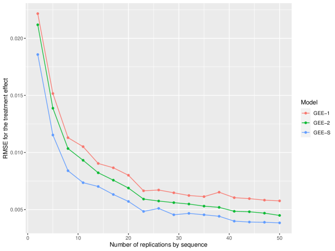
Figure 1: RMSE for the estimate of $\beta_{1}=0.5$ in each of the models

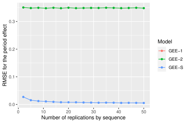
Figure 2: RMSE for the estimate of $\beta_{2}=3$ in each of the models

Each scenario is simulated 1000 times with an autoregressive correlation matrix of order 1, and for each component of $\boldsymbol{\beta}$, the following goodness of fit measures are obtained: 1) The root mean square error $RMSE=\sqrt{(\hat{\beta}_{i}-\beta_{i})^{2}}$ and 2) the percentage of times the hypothesis $H_{0}:\;\beta_{1}=0.5$, $H_{0}:\;\beta_{1}=1$ and $H_{0}:\;\beta_{1}=2$ are not rejected at 95% confidence bands.

Further, for each scenario, the following three models are fitted: 1) A model defined by Equation (3) which is denoted by GEE-S, 2) a GEE model where the effect of time is linear which is denoted by GEE-1 and 3) a GEE model with quadratic time effect which is denoted by GEE-2.

Table 8 shows the coverage obtained for three different values of the treatment effect ($\beta_{1}$) using 95% confidence intervals. A coverage close to 95% is observed for replicate sizes greater than 8 in the model with Splines; the other two models show coverage equal to 100%, that is, these models over-estimate the variance of the estimated treatment effects. This is confirmed in Figure 1, where it is shown that although the RMSE of each model decreases as the number of replicas increases, it does so faster in the Splines model.

On the other hand, Table 7 shows the coverage obtained for the period effect ($\beta_{2}$ and $\beta_{3}$) using 95% confidence intervals. The models without splines have a coverage of zero in all the scenarios because the effect of the period is confused with the time effect in the estimation equation, which is also observed in Figure 2. The confidence intervals obtained from splines have a coverage close to 95% when there were 11 experimental units per sequence, see Figure 2. Results from this simulation suggest that when time effects are not linear or quadratic, models that do not use splines overestimate the variance of the treatment effects, and these fail to estimate unbiasedly the period effects. This leads to erroneous conclusions about the effectiveness of the sequences and treatments.

5 Application

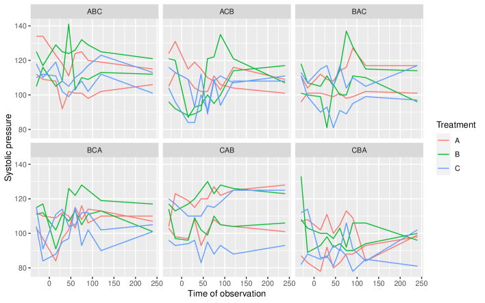
Figure 3: Blood systolic pressure (mmHg) observed through time (minutes)

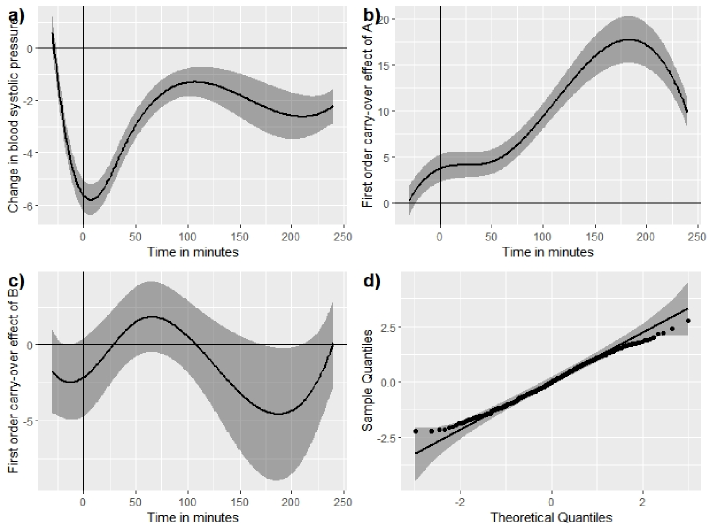
Figure 4: a) Changes of blood systolic pressure through time using splines, b) First order carry-over effect of the treatment A through time using splines, c) First order carry-over effect of the treatment B through time using splines, and d) Residuals normal probability plot. All figures present 95% confidence intervals and are based on the cross-over design of Table 1

Two studies are presented below where the model proposed in (3) is used. In both the software R Core Team (2022) is used through adaptation of the package geeM built by McDaniel et al. (2013).

5.1 Systolic pressure data

	Estimate	Std.err	Wald	Pr($>|W|$)
Intercept	109.35	3.17	1192.44	0.00
BaseLine	3.85	1.47	6.82	0.01
Period 2	-0.88	3.49	0.06	0.80
Period 3	-3.22	3.60	0.80	0.37
Treatment B	0.70	3.04	0.05	0.82
Treatment C	-5.95	3.60	2.73	0.01

Table 3: Analysis of blood systolic pressure data using GEE-Splines

Jones and Kenward (2015, pg 204) describes the following crossover design: 3 treatments for blood pressure control are used; treatment A consists of a 20 mg dose of a test drug, treatment B is a 40 mg dose of the same drug, and treatment C is a placebo. 6 sequences of three periods (ABC, ACB, BCA, BAC, CAB, CBA) are organized and each one is applied to two individuals. In each application period, 10 successive measurements of systolic blood pressure are made: 30 and 15 minutes before the application, and 15, 30, 45, 60, 75, 90, 120 and 240 minutes after the application, as shown in Table 1 and the profile is shown in Figure 3.

Figure 4.a) shows the smoothed function corresponding to the effect of time on blood pressure; it is based on the moments of measurement for the design in Table 1. That is, 30 and 15 minutes before the application, and 15, 30, 45, 60, 75, 90, 120 and 240 minutes after the application. Additionally, Figure 4.a) shows the average function and its 95% confidence bands obtained through cross-validation. A wide drop in pressure is observed from the time that the patient expects to receive treatment, then it rises a little and remains stable. This behavior is widely studied in medical settings, see Stergiou et al. (1998) and Fanelli et al. (2021).

The carry-over effects of treatment A and treatment B are observed in Figures 4.b) and 4.c) respectively. The value for the carry-over effect of A is positive and increases over time, which implies that having applied placebo in a previous period will generate higher blood pressure values in the following application period. For treatment B (medium dose), the carry-over effect is close to zero; therefore, it is a negligible effect for the next treatment. Table 3 shows the parametric effects, their standard error and the Wald statistic built from matrices (14) and (15). It is worth highlighting the positive effect of the baseline, i.e., people have the highest blood pressure before starting the study. The periods are not significant i.e., the conditions were similar across the study, and these had a significant effect on pressure of treatment C on pressure reduction.

Finally, Figure 4.d) shows the confidence bands for the quantiles of the standardized residuals defined in (17) compared to a standard normal distribution.These residuals seem to fit the normal distribution assumption.

5.2 Blood Sugar levels in Rabbits

Kenward and Roger (2009) described the following cross-over experiment: two treatments for the control of diabetes A and B were used, two sequences of four periods (ABAB, BABA) are organized and each one was applied to twelve female rabbits; each period lasted one week. In each period, at the middle of the week, five successive measurements of the blood sugar level were taken: 0, 1.5, 3, 4.5 and 6 hours after the application, as shown in Table 4 and Figure 5.

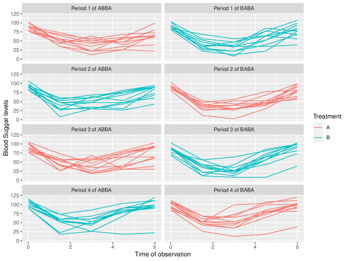
Figure 5: Blood sugar levels (mg/dL) in rabbits through time (hours)

Sequence	Period 1	Period 2
(1) ABAB Ind 1 $\vdots$ Ind 11	5 observations $\vdots$ 5 observations	5 observations $\vdots$ 5 observations
(2) BABA Ind 12 $\vdots$ Ind 22	5 observations $\vdots$ 5 observations	5 observations $\vdots$ 5 observations

Table 4: Structure of the cross-over design of blood sugar levels in rabbits

Assuming that the distribution of blood sugar levels is normal, a first analysis was run. When making the normal probability plot of the standardized residuals defined in (17), it is observed that they do not fit correctly to a standard normal distribution, as seen in Figure 6 and the assumption is rejected. A gamma distribution is then explored, with loglinear linkage. Figure 7 c) shows the confidence bands for the quantiles of the standardized residuals defined in (17) against a standard normal distribution, concluding that the gamma distribution assumption is adequate. To compare the distributions, three models are made to analyze the response variable: i) Under the assumption of normality, ii) Under the assumption of gamma distribution and inverse link, and iii) under the assumption of gamma distribution and a loglinear link. In each one, the QIC is calculated and shows in Table 5.

Model	QIC
Normal	3927.6
Gamma Inverse	3732.22
Gamma Log	3728.5

Table 5: QIC for the three fitted models to the response of blood sugar levels in rabbits

Therefore, all the analysis is carried out with the gamma distribution assumption and the loglinear model given by:

$$\ln(\mu_{ijk}) =\boldsymbol{x}_{ijk}^{T}\boldsymbol{\beta}+f_{1}(\boldsymbol{Z}_{1ijk})+f_{2}(\boldsymbol{Z}_{2ijk})$$

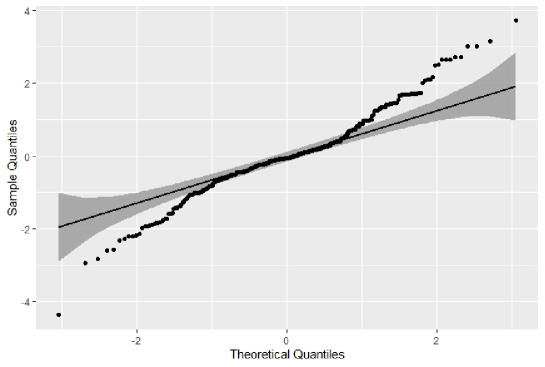
Figure 6: Residuals normal probability plot with 95% confidence intervals of the residuals obtained assuming a Gaussian distribution of the response in the cross-over design of the Table 4

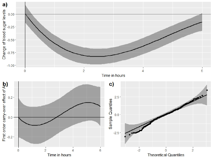
Figure 7: a) Change of blood sugar levels through time using splines, b) First order carry-over effect of the treatment A through time using splines, and c) Residuals normal probability plot. All figures present 95% confidence intervals and are based on the cross-over design of the Table 4 with linear log link for the mean of an assumed gamma distribution

The spline-smoothed function for the time effect on the blood sugar level of female rabbits is shown in Figure 7a), it is based on the moments of measurement for the design of Table 4; the average functions and their 95% confidence bands, estimated through cross validation are presented. A marked decrease in levels is observed until 2 hours, and then an increase until hour 6. In Jones and Kenward (2015, pag 237) it was stated that there was an effect of the hours, but its form is not explained. However, the proposed model permits to describe this effect. Figure 7.b) shows the carry-over effects of treatment A over treatment B. This increases over time, but it is close to 0, which implies that having applied A in a previous period will not significantly affect the next application period. The parametric effects, their standard error and the Wald statistic constructed with matrices (14) and (15) are presented in Table 6.

	Estimate	Std.err	Wald	Pr($>|W|$)
Intercept	4.47	0.05	9734.05	0.00
Period 2	0.01	0.06	0.00	0.96
Period 3	-0.01	0.06	0.01	0.94
Period 4	0.25	0.06	16.68	0.00
Treatment B	-0.02	0.04	0.28	0.60

Table 6: Analysis of blood sugar levels data using GEE-Splines

It is noteworthy that there are no significant effects of treatment, similar to that obtained by Jones and Kenward (2015) and Kenward and Roger (2009), but there is an positive effect of period four. This behavior was not analyzed in previous studies and can be seen as increased insulin resistance by blood cells; similar to behaviors reported by Ning et al. (2015) and Da Silva et al. (2020).

In the modeling of blood pressure, the normal distribution presents a better performance than the gamma distribution, while in blood sugar levels, the gamma distribution achieves a better fit than the normal distribution. Choosing the most suitable distribution is desirable, because the standard errors of each estimator of the parametric effects of the model are smaller. In addition, the Pearson residuals show a behavior that conforms to a standard normal in both cases, guaranteeing that the model specification is adequate.

These applications show the importance of the semiparametric approach proposed in this paper to model time and carry-over effects in crossover designs with repeated measures within periods. Also, it complements the simulation study, where the efficiency of the proposed model over conventional models was verified.

6 Conclusions

The proposed methodology provides highly desirable properties of the resulting estimators. It allows doing asymptotic inference and better to model temporal carry-over behaviors that would be intractable in parametric scenarios, as in the case of blood pressure data, where these effects do not present the typical polynomial effects. In addition, detecting these carry-over effects of the placebo allows estimating treatment effects with greater precision and unbiasedness, which is basically the objective of any crossover design.
In the insulin data in rabbits, the behavior of the estimated effect of time is similar to a quadratic form, which shows that this methodological proposal encompasses the classical parametric temporal models with linear or cubic polynomials. In addition, the GEE allow modeling a large number of response variables, not only normal or continuous, but also counts or proportions of successes. In the simulation, the inferential gain is evidenced in terms of coverage and control of the type I and II error of the hypothesis tests associated with the parameters of interest; that is, treatment and period effects when the temporal behavior is sinusoidal. While linear or quadratic models lose efficiency and unbiasedness; therefore, estimation with splines is presented as a useful tool for this type of design.
The asymptotic properties of the estimators allow an agile and fast verification of the model, because its similarity with weighted least squares is demonstrated. Therefore, the adaptation of widely used diagnostic tests in normal linear models can be used.

Appendix A Appendix 1

Proof.

Let

$$\boldsymbol{\theta}(\boldsymbol{\hat{\beta}},\boldsymbol{\hat{\alpha}}_{1},\boldsymbol{\hat{\alpha}}_{2})=\begin{pmatrix}\boldsymbol{B}_{n}^{\frac{1}{2}}(\boldsymbol{\hat{\beta}}-\boldsymbol{\beta})\\ \sqrt{n}\boldsymbol{H}_{1n}(\boldsymbol{\hat{\alpha}}_{1}-\boldsymbol{\alpha}_{1})+\sqrt{n}\boldsymbol{H}_{1n}\boldsymbol{W}_{1}^{T}\boldsymbol{X}(\boldsymbol{\hat{\beta}}-\boldsymbol{\beta})\\ \sqrt{n}\boldsymbol{H}_{2n}(\boldsymbol{\hat{\alpha}}_{2}-\boldsymbol{\alpha}_{2})+\sqrt{n}\boldsymbol{H}_{2n}\boldsymbol{W}_{2}^{T}\boldsymbol{X}(\boldsymbol{\hat{\beta}}-\boldsymbol{\beta})\\ \end{pmatrix}$$ (20)

with $\boldsymbol{B}$ as in Equation (15), and

$$\boldsymbol{W}_{1} =\left(\boldsymbol{\pi}_{11},\ldots,\boldsymbol{\pi}_{1n}\right),\;\boldsymbol{\pi}_{1i}=(\pi(\boldsymbol{Z}_{1i11}),\ldots,\pi(\boldsymbol{Z}_{1ijn_{ij}}))$$

$$\boldsymbol{W}_{2} =\left(\boldsymbol{\pi}_{21},\ldots,\boldsymbol{\pi}_{2n}\right),\;\boldsymbol{\pi}_{2i}=(\pi(\boldsymbol{Z}_{2i11}),\ldots,\pi(\boldsymbol{Z}_{2ijn_{ij}}))$$

$$\boldsymbol{H}_{1n} =n\boldsymbol{W}_{1}^{T}\boldsymbol{W}_{1},\;\boldsymbol{H}_{2n}=n\boldsymbol{W}_{2}^{T}\boldsymbol{W}_{2}$$ (21)

$$\boldsymbol{X} =(\boldsymbol{x}_{1}^{T},\ldots,\boldsymbol{x}_{n}^{T}),\;\pi(t)=\{s_{1}(t),\ldots,s_{m}(t)\}$$

Following ideas presented in Speckman (1988) to guarantee that both $\boldsymbol{X}$ and $\boldsymbol{Z}_{ij}$ have finite second moments, we assume that there exists a random variables $\delta_{ijk}$, with $E(\delta_{ijk})=0$ and $Var(\delta_{ijk})\leq\infty$ and continuous functions $g_{1}\ldots g_{m}$ such that:

$$x_{ijkl}=g_{l}(\boldsymbol{Z}_{ijk})+\delta_{ijkl}\qquad 1\leq i\leq n,\;1\leq j\leq P,\;1\leq k\leq n_{ij},\;1\leq l\leq dim\left(\boldsymbol{\beta}\right)$$ (22)

These functions allow modeling the possible relationship between the vector of variables associated to the parametric effects and the measurement times within each period. Let $\boldsymbol{X}_{ij}=(x_{ij1},\ldots,x_{ijn_{ij}})$ be the parametric effects design matrix, then the following properties hold:

• The succession $\{n_{ij}\}$ is bounded for all $1\leq i\leq n$ and $1\leq j\leq P$, that is:

  $$max(n_{ij})<\infty$$

• Since $Y_{ijk}$ is a random variable that belongs to the exponential family and due to the definition of the generalized estimation equations in Liang and Zeger (1986), and by Lemmma 5.3 given in Lehmann and Casella (2006, pag 116), then

  $$E(\boldsymbol{u}_{1i}) =E\left(\boldsymbol{y}_{i}-\boldsymbol{\mu}_{i}\left[\boldsymbol{X}_{i}\boldsymbol{\beta},\sum_{b=1}^{m}\alpha_{1b}s_{b}(t),\hat{f}_{2}(\boldsymbol{Z}_{2i})\right]\right)=0$$

  Therefore, the expected value of (7) is:

  $$E(U_{1}(\boldsymbol{\epsilon}_{i},t)) =E\left\{\sum_{i=1}^{n}\left\{diag\left(\frac{\partial\mu_{ijk}}{\partial\boldsymbol{\alpha}_{1}}\right)\right\}_{i}\frac{\boldsymbol{V}^{-1}_{1i}}{\phi}\left(\boldsymbol{y}_{i}-\boldsymbol{\mu}_{i}\left[\boldsymbol{X}_{i}\boldsymbol{\beta},\sum_{b=1}^{m}\alpha_{1b}s_{b}(t),\hat{f}_{2}(\boldsymbol{Z}_{2i})\right]\right)\right\}$$

  $$=\sum_{i=1}^{n}\left\{diag\left(\frac{\partial\mu_{ijk}}{\partial\boldsymbol{\alpha}_{1}}\right)\right\}_{i}\frac{\boldsymbol{V}^{-1}_{1i}}{\phi}E\left(\boldsymbol{y}_{i}-\boldsymbol{\mu}_{i}\left[\boldsymbol{X}_{i}\boldsymbol{\beta},\sum_{b=1}^{m}\alpha_{1b}s_{b}(t),\hat{f}_{2}(\boldsymbol{Z}_{2i})\right]\right)$$

  $$=0\,\forall t\in\mathbb{R}$$

  Analogous results are obtained for equations (8), (9) and (10). As $E(Y_{ijk}^{2})<\infty$ and the density function satisfies the regularity conditions then, by Theorems 1 and 2 of Pan (2001b) and by theorem 2.6 of Lehmann and Casella (2006, pg 440), for Equation (7), it follows that:

  $$0<E\left(U_{1}(\boldsymbol{\epsilon}_{i},t)U_{1}(\boldsymbol{\epsilon}_{i},t)^{T}\right)<\infty$$

  Similarly, for equations (8), (9) and (10), the following results are obtained:

  $$E(U_{2}(\boldsymbol{\epsilon}_{i},t)) =0,\qquad 0<E\left(U_{2}(\boldsymbol{\epsilon}_{i},t)U_{2}(\boldsymbol{\epsilon}_{i},t)^{T}\right)<\infty,\;\forall t\in\mathbb{R},$$

  $$E(U_{3}(\boldsymbol{\epsilon}_{i},t)) =0,\qquad 0<E\left(U_{3}(\boldsymbol{\epsilon}_{i},t)U_{3}(\boldsymbol{\epsilon}_{i},t)^{T}\right)<\infty,\;\forall t\in\mathbb{R},$$

  $$E(U_{4}(\boldsymbol{\epsilon}_{i})) =0,\qquad 0<E\left(U_{4}(\boldsymbol{\epsilon}_{i})U_{4}(\boldsymbol{\epsilon}_{i})^{T}\right)<\infty,$$

  where $\boldsymbol{\epsilon}_{i}=(\epsilon_{i11},\ldots,\epsilon_{in_{iP}})=\boldsymbol{z}_{i}-\boldsymbol{\hat{z}}_{i}$, with $\boldsymbol{z}_{i}$ defined the equation (13).

• According to theorem 2.6 of Lehmann and Casella (2006, pg 441), there exist $\{b_{1ijk}\}$, $\{b_{2ijk}\}$ and $\{b_{3ijk}\}$ with $0<inf_{ijk}(b_{ijk})\leq sup_{ijk}(b_{ijk})<\infty$, $0<inf_{ijk}(b_{ijk})\leq sup_{ijk}(b_{ijk})<\infty$ and $0<inf_{ijk}(b_{ijk})\leq sup_{ijk}(b_{ijk})<\infty$ such that when $s\to 0$, the following properties hold, respectively::

  $$\sup_{ijk}\left|E(U_{1}(\boldsymbol{\epsilon}_{ijk}+s,t))-b_{1ijk}s\right| =O(s^{2}),\;\forall t\in\mathbb{R},$$

  $$\sup_{ijk}\left|E(U_{2}(\boldsymbol{\epsilon}_{ijk}+s,t))-b_{2ijk}s\right| =O(s^{2}),\;\forall t\in\mathbb{R},$$

  $$\sup_{ijk}\left|E(U_{3}(\boldsymbol{\epsilon}_{ijk}+s))-b_{3ijk}s\right| =O(s^{2}),$$ (23)

  Also, when $s\to 0$, exist constants $c>0$ and, $C<\infty$ such that:

  $$\sup_{ijk}\left\{E(U_{1}(\boldsymbol{\epsilon}_{ijk}+s,t)-U_{1}(\boldsymbol{\epsilon}_{ijk},t))^{2}\right\}\leq C|s|,\;\forall t\in\mathbb{R}$$

  $$\sup_{ijk}\left\{E(U_{2}(\boldsymbol{\epsilon}_{ijk}+s,t)-U_{2}(\boldsymbol{\epsilon}_{ijk},t))^{2}\right\}\leq C|s|,\;\forall t\in\mathbb{R}$$

  $$\sup_{ijk}\left\{E(U_{3}(\boldsymbol{\epsilon}_{ijk}+s)-U_{1}(\boldsymbol{\epsilon}_{ijk}))^{2}\right\}\leq C|s|$$

  Furthermore, $|U_{1}(\nu+\eta,t)-U_{1}(\nu,t)-U_{1}(\eta,t)|\leq c$, $|U_{2}(\nu+\eta,t)-U_{2}(\nu,t)-U_{2}(\eta,t)|\leq c$ and $|U_{3}(\nu+\eta)-U_{3}(\nu)-U_{3}(\eta)|\leq c$ for any $|\eta|\leq s$ and $\nu,t\in\mathbb{R}.$

• Let $\boldsymbol{\Delta}_{n}$ be a diagonal matrix with elements $\delta_{ijkl}$ defined in equation (22) and let $\boldsymbol{\Lambda}_{n}$ be a diagonal matrix with elements $b_{3ijk}$ defined in equation (23), then by definition of the random variables $\delta_{ijkl}$ it follows that:

  $$E(\boldsymbol{\Delta}_{n})=0\text{ y }\sup_{n}\left\{\frac{1}{n}E(||\boldsymbol{\Delta}_{n}||^{2})\right\}<\infty$$

  Since, $\boldsymbol{\Gamma}_{n}$ is a block diagonal matrix with elements $A_{i}=E\left(U_{3}(\boldsymbol{\epsilon}_{i})U_{3}(\boldsymbol{\epsilon}_{i})^{T}\right)$, then by the theorem 1 in Pan (2001b),

  $$\frac{1}{n}\boldsymbol{\Delta}_{n}^{T}\boldsymbol{\Gamma}_{n}\boldsymbol{\Delta}_{n}\overset{p}{\to}\boldsymbol{B}$$ (24)

  $$\frac{1}{n}\boldsymbol{\Delta}_{n}^{T}\boldsymbol{\Lambda}_{n}\boldsymbol{\Delta}_{n}\overset{p}{\to}\boldsymbol{A}$$ (25)

• The matrices $\boldsymbol{H}_{1n}$ y $\boldsymbol{H}_{2n}$ defined in (21) are symmetric and positive definite, so they have square root (Bunch and Hopcroft, 1974). Let $\boldsymbol{H}_{1n}^{\frac{1}{2}}$ and $\boldsymbol{H}_{2n}^{\frac{1}{2}}$ be those square roots, respectively. Also, as a kernel spline forms a linearly independent basis, and by Theorem 21.5.1 of Harville (1997, pg 537), $\boldsymbol{H}_{1n}^{\frac{1}{2}}$ and $\boldsymbol{H}_{2n}^{\frac{1}{2}}$ are non-singular matrices and their eigenvalues are bounded between zero and infinity.

With the previous results and using Theorem 1 and Theorem 2 of He et al. (2002), the following results are obtained:

$$\frac{1}{n}\sum_{i=1}^{n}\sum_{j=1}^{n_{i}}\left\{\sum_{b=1}^{m}\hat{\alpha}_{1b}s_{b}(\boldsymbol{Z}_{1ijk})-f_{1}(\boldsymbol{Z}_{1ijk})\right\}^{2}=O\left(n^{-\frac{2r}{(2r+1)}}\right)$$ (26)

$$\frac{1}{n}\sum_{i=1}^{n}\sum_{j=1}^{n_{i}}\left\{\sum_{b=1}^{m}\hat{\alpha}_{1b}s_{b}(\boldsymbol{Z}_{2ijk})-f_{2}(\boldsymbol{Z}_{2ijk})\right\}^{2}=O\left(n^{-\frac{2r}{(2r+1)}}\right)$$ (27)

$$\sqrt{n}(\hat{\boldsymbol{\beta}}-\boldsymbol{\beta})\rightarrow N(0,\boldsymbol{A}^{-1}\boldsymbol{B}\boldsymbol{A}^{-1})$$ (28)

where the matrices $\boldsymbol{A}$ and $\boldsymbol{B}$ are defined in Equations (14) and (15), respectively. ∎

Appendix B Appendix 2

	$H_{0}:\;\beta_{2}=3$	$H_{0}:\;\beta_{3}=3$
n 2 5 8 11 14 17 20 23 26 29 32 35 38 41 44 47 50	GEE-S GEE-1 GEE2 0.79 0.44 0.44 0.84 0.00 0.00 0.94 0.00 0.00 0.94 0.00 0.00 0.92 0.00 0.00 0.94 0.00 0.00 0.94 0.00 0.00 0.94 0.00 0.00 0.94 0.00 0.00 0.92 0.00 0.00 0.95 0.00 0.00 0.92 0.00 0.00 0.92 0.00 0.00 0.95 0.00 0.00 0.93 0.00 0.00 0.93 0.00 0.00 0.94 0.00 0.00	GEE-S GEE-1 GEE2 0.80 0.50 0.51 0.89 0.00 0.00 0.90 0.00 0.00 0.92 0.00 0.00 0.92 0.00 0.00 0.94 0.00 0.00 0.95 0.00 0.00 0.95 0.00 0.00 0.95 0.00 0.00 0.94 0.00 0.00 0.95 0.00 0.00 0.92 0.00 0.00 0.92 0.00 0.00 0.92 0.00 0.00 0.94 0.00 0.00 0.92 0.00 0.00 0.90 0.00 0.00

Table 7: Proportion of times that hypothesis $H_{0}$ is not rejected for some values of $\beta_{2}$ and $\beta_{3}$ (the period effects)

	$H_{0}:\;\beta_{1}=0.5$	$H_{0}:\;\beta_{1}=1$	$H_{0}:\;\beta_{1}=2$
n 2 5 8 11 14 17 20 23 26 29 32 35 38 41 44 47 50	GEE-S GEE-1 GEE2 0.88 1.00 1.00 0.90 1.00 1.00 0.93 1.00 1.00 0.92 1.00 1.00 0.95 1.00 1.00 0.94 1.00 1.00 0.95 1.00 1.00 0.95 1.00 1.00 0.96 1.00 1.00 0.96 1.00 1.00 0.95 1.00 1.00 0.95 1.00 1.00 0.96 1.00 1.00 0.94 1.00 1.00 0.95 1.00 1.00 0.97 1.00 1.00 0.95 1.00 1.00	GEE-S GEE-1 GEE2 0.82 1.00 1.00 0.92 1.00 1.00 0.96 1.00 1.00 0.96 1.00 1.00 0.94 1.00 1.00 0.94 1.00 1.00 0.94 1.00 1.00 0.96 1.00 1.00 0.96 1.00 1.00 0.97 1.00 1.00 0.94 1.00 1.00 0.94 1.00 1.00 0.93 1.00 1.00 0.94 1.00 1.00 0.94 1.00 1.00 0.95 1.00 1.00 0.94 1.00 1.00	GEE-S GEE-1 GEE2 0.85 1.00 1.00 0.88 1.00 1.00 0.93 1.00 1.00 0.92 1.00 1.00 0.96 1.00 1.00 0.94 1.00 1.00 0.94 1.00 1.00 0.96 1.00 1.00 0.97 1.00 1.00 0.93 1.00 1.00 0.97 1.00 1.00 0.92 1.00 1.00 0.94 1.00 1.00 0.98 1.00 1.00 0.93 1.00 1.00 0.93 1.00 1.00 0.97 1.00 1.00

Table 8: Proportion of times that hypothesis $H_{0}$ is not rejected for some values of $\beta_{1}$ (the treatment effect)

References

- Biabani et al. (2018) Biabani, M., Farrell, M., Zoghi, M., Egan, G., and Jaberzadeh, S. (2018). Crossover design in transcranial direct current stimulation studies on motor learning: potential pitfalls and difficulties in interpretation of findings. Reviews in the Neurosciences, 29(4), 463–473.
- Bunch and Hopcroft (1974) Bunch, J. R. and Hopcroft, J. E. (1974). Triangular factorization and inversion by fast matrix multiplication. Mathematics of Computation, 28(125), 231–236.
- Curtin (2017) Curtin, F. (2017). Meta-analysis combining parallel and crossover trials using generalised estimating equation method. Research Synthesis Methods, 8(3), 312–320.
- Da Silva et al. (2020) Da Silva, A. A., do Carmo, J. M., Li, X., Wang, Z., Mouton, A. J., and Hall, J. E. (2020). Role of hyperinsulinemia and insulin resistance in hypertension: metabolic syndrome revisited. Canadian Journal of Cardiology, 36(5), 671–682.
- Diaz et al. (2013) Diaz, F. J., Berg, M. J., Krebill, R., Welty, T., Gidal, B. E., Alloway, R., and Privitera, M. (2013). Random-effects linear modeling and sample size tables for two special crossover designs of average bioequivalence studies: the four-period, two-sequence, two-formulation and six-period, three-sequence, three-formulation designs. Clinical pharmacokinetics, 52(12), 1033–1043.
- Dubois et al. (2011) Dubois, A., Lavielle, M., Gsteiger, S., Pigeolet, E., and Mentré, F. (2011). Model-based analyses of bioequivalence crossover trials using the stochastic approximation expectation maximisation algorithm. Statistics in Medicine, 30(21), 2582–2600.
- Fanelli et al. (2021) Fanelli, E., Di Monaco, S., Pappaccogli, M., Eula, E., Fasano, C., Bertello, C., Veglio, F., and Rabbia, F. (2021). Comparison of nurse attended and unattended automated office blood pressure with conventional measurement techniques in clinical practice. Journal of Human Hypertension, pages 1–6.
- Forbes et al. (2015) Forbes, A. B., Akram, M., Pilcher, D., Cooper, J., and Bellomo, R. (2015). Cluster randomised crossover trials with binary data and unbalanced cluster sizes: Application to studies of near-universal interventions in intensive care. Clinical Trials, 12(1), 34–44.
- Harville (1997) Harville, D. A. (1997). Matrix algebra from a statistician’s perspective. Springer, New York.
- He et al. (2002) He, X., Zhu, Z.-Y., and Fung, W.-K. (2002). Estimation in a semiparametric model for longitudinal data with unspecified dependence structure. Biometrika, 89(3), 579–590.
- Hinkelmann and Kempthorne (2005) Hinkelmann, K. and Kempthorne, O. (2005). Design and Analysis of Experiments. Wiley series in probability and mathematical statistics. Applied probability and statistics. Wiley, New York, Vol 2.
- Jones and Kenward (2015) Jones, B. and Kenward, M. G. (2015). Design and Analysis of Cross-Over Trials Third Edition. Chapman & Hall/CRC, Boca Raton.
- Kenward and Roger (2009) Kenward, M. G. and Roger, J. H. (2009). The use of baseline covariates in crossover studies. Biostatistics, 11(1), 1–17. ISSN 1465-4644.
- Kitchenham et al. (2018) Kitchenham, B., Madeyski, L., and Curtin, F. (2018). Corrections to effect size variances for continuous outcomes of cross-over clinical trials. Statistics in Medicine, 37(2), 320–323.
- Lehmann and Casella (2006) Lehmann, E. L. and Casella, G. (2006). Theory of point estimation. Springer Science & Business Media.
- Li et al. (2018) Li, F., Forbes, A. B., Turner, E. L., and Preisser, J. S. (2018). Power and sample size requirements for gee analyses of cluster randomized crossover trials. Statistics in Medicine.
- Liang and Zeger (1986) Liang, K.-Y. and Zeger, S. L. (1986). Longitudinal data analysis using generalized linear models. Biometrika, 73(1), 13–22.
- Lin and Carroll (2001) Lin, X. and Carroll, R. J. (2001). Semiparametric regression for clustered data using generalized estimating equations. Journal of the American Statistical Association, 96(455), 1045–1056.
- Liu and Li (2016) Liu, F. and Li, Q. (2016). A bayesian model for joint analysis of multivariate repeated measures and time to event data in crossover trials. Statistical Methods in Medical Research, 25(5), 2180–2192.
- Madeyski and Kitchenham (2018) Madeyski, L. and Kitchenham, B. (2018). Effect sizes and their variance for ab/ba crossover design studies. Empirical Software Engineering, 23(4), 1982–2017.
- McDaniel et al. (2013) McDaniel, L. S., Henderson, N. C., and Rathouz, P. J. (2013). Fast pure R implementation of GEE: application of the Matrix package. The R Journal, 5, 181–187. URL https://journal.r-project.org/archive/2013-1/mcdaniel-henderson-rathouz.pdf.
- Ning et al. (2015) Ning, B., Wang, X., Yu, Y., Waqar, A. B., Yu, Q., Koike, T., Shiomi, M., Liu, E., Wang, Y., and Fan, J. (2015). High-fructose and high-fat diet-induced insulin resistance enhances atherosclerosis in watanabe heritable hyperlipidemic rabbits. Nutrition & metabolism, 12(1), 1–11.
- Oh et al. (2003) Oh, H. S., Ko, S.-g., and Oh, M.-S. (2003). A bayesian approach to assessing population bioequivalence in a 2 2 2 crossover design. Journal of Applied Statistics, 30(8), 881–891.
- Pan (2001a) Pan, W. (2001a). Akaike’s information criterion in generalized estimating equations. Biometrics, 57, 120–125.
- Pan (2001b) Pan, W. (2001b). On the robust variance estimator in generalised estimating equations. Biometrika, 88(3), 901–906.
- Patterson (1951) Patterson, H. D. (1951). Change-over trials. Journal of the Royal Statistical Society. Series B (Methodological), 13, 256–271.
- R Core Team (2022) R Core Team (2022). R: A Language and Environment for Statistical Computing. R Foundation for Statistical Computing, Vienna, Austria. URL https://www.R-project.org/.
- Shkedy et al. (2005) Shkedy, Z., Molenberghs, G., Craenendonck, H. V., Steckler, T., and Bijnens, L. (2005). A hierarchical binomial-poisson model for the analysis of a crossover design for correlated binary data when the number of trials is dose-dependent. Journal of Biopharmaceutical Statistics, 15(2), 225–239.
- Speckman (1988) Speckman, P. (1988). Kernel smoothing in partial linear models. Journal of the Royal Statistical Society: Series B (Methodological), 50(3), 413–436.
- Stergiou et al. (1998) Stergiou, G. S., Zourbaki, A. S., Skeva, I. I., and Mountokalakis, T. D. (1998). White coat effect detected using self-monitoring of blood pressure at home: comparison with ambulatory blood pressure. American Journal of Hypertension, 11(7), 820–827.
- Stoklosa and Warton (2018) Stoklosa, J. and Warton, D. I. (2018). A generalized estimating equation approach to multivariate adaptive regression splines. Journal of Computational and Graphical Statistics, 27(1), 245–253.
- Tsuyuguchi et al. (2020) Tsuyuguchi, A. B., Paula, G. A., and Barros, M. (2020). Analysis of correlated birnbaum–saunders data based on estimating equations. TEST, 29(3), 661–681.
- Vegas et al. (2016) Vegas, S., Apa, C., and Juristo, N. (2016). Crossover designs in software engineering experiments: Benefits and perils. IEEE Transactions on Software Engineering, 42(2), 120–135.
- Wild and Yee (1996) Wild, C. and Yee, T. (1996). Additive extensions to generalized estimating equation methods. Journal of the Royal Statistical Society: Series B (Methodological), 58(4), 711–725.
- Yang and Niu (2021) Yang, L. and Niu, X.-F. (2021). Semi-parametric models for longitudinal data analysis. Journal of Finance and Economics, 9(3), 93–105.
- Yu and Peace (2012) Yu, L. and Peace, K. E. (2012). Spline nonparametric quasi-likelihood regression within the frame of the accelerated failure time model. Computational Statistics & Data Analysis, 56(9), 2675–2687.