The phase curve and the geometric albedo of WASP-43b measured with CHEOPS, TESS and HST WFC3/UVIS

Abstract

Context. Observations of the phase curves and secondary eclipses of extrasolar planets provide a window on the composition and thermal structure of the planetary atmospheres. For example, the photometric observations of secondary eclipses lead to the measurement of the planetary geometric albedo $A_{g}$, which is an indicator of the presence of clouds in the atmosphere.

Aims. In this work we aim to measure the $A_{g}$ in the optical domain of WASP-43b, a moderately irradiated giant planet with an equilibrium temperature of $\sim$1400 K.

Methods. To this purpose, we analyze the secondary eclipse light curves collected by CHEOPS, together with TESS observations of the system and the publicly available photometry obtained with HST WFC3/UVIS. We also analyze the archival infrared observations of the eclipses and retrieve the thermal emission spectrum of the planet. By extrapolating the thermal spectrum to the optical bands, we correct the optical eclipses for thermal emission and derive the optical $A_{g}$.

Results. The fit of the optical data leads to a marginal detection of the phase curve signal, characterized by an amplitude of $160\pm 60$ ppm and 80${}^{+60}_{-50}$ ppm in the CHEOPS and TESS passband respectively, with an eastward phase shift of $\sim 50^{\circ}$ (1.5$\sigma$ detection). The analysis of the infrared data suggests a non-inverted thermal profile and solar-like metallicity. The combination of optical and infrared analysis allows us to derive an upper limit for the optical albedo of A_g$<0.087$ with a confidence of 99.9%.

Conclusions. Our analysis of the atmosphere of WASP-43b places this planet in the sample of irradiated hot Jupiters, with monotonic temperature-pressure profile and no indication of condensation of reflective clouds on the planetary dayside.

1 Introduction

Phase curve and secondary eclipse observations are among the main avenues to characterize extra-solar planet atmospheres, as they provide a window on their composition and thermal structure. Thanks to these observations, we can probe planetary brightness temperatures at different wavelengths, and constrain molecular abundances at different pressure levels (e.g. Alonso et al. 2009; Kreidberg et al. 2014; Stevenson et al. 2014; Foote et al. 2022). Additionally, secondary eclipse depth measurements are sensitive to temperature gradients with atmospheric pressure (i.e. altitude), to the presence of molecules which absorb ultraviolet-to-visible stellar radiation, as well as to temperature inversion that manifests through emission lines (e.g. Mansfield et al. 2018; Baxter et al. 2020; Garhart et al. 2020, and references therein).

One of the main parameters obtained by eclipse depth measurements is the planetary albedo, which describes the body’s surface or atmosphere reflectivity (Seager 2010). This latter, in turn, is an indicator of the presence of reflective clouds, currently a poorly constrained component in our understanding of exoplanet atmospheres and an important source of limitation in our measurement of molecular mixing ratios (e.g. Sing et al. 2016; Pinhas et al. 2019, and references therein).

Unlike most ultra-short period (P $\leq$1 day) Hot Jupiters, WASP-43b is only moderately irradiated to an equilibrium temperature of $\sim 1400$ K. It thus resides in a temperature range where cloud condensation can occur on the planetary dayside, setting the object apart from ultra-hot Jupiters with extremely hot and therefore likely clear daysides (e.g. Helling et al. 2021). In an effort to understand its atmospheric physical-chemical environment, this planet has been targeted by Spitzer (e.g. Stevenson et al. 2017), HST (e.g. Stevenson et al. 2014; Fraine et al. 2021) and ground-based telescopes (Weaver et al. 2019). In particular, 3D Global Circulation Models with $5\times$ solar metallicity without clouds match the HST WFC3/G141 infrared observations of the planetary dayside (Kataria et al. 2015). However, later 3D atmospheric models including cloud condensation processes by Helling et al. (2020) and Venot et al. (2020) predict the presence of several species of clouds (most importantly silicate and metal-oxide components) on the dayside of WASP-43b. If present at observable altitudes, their reflectance would contribute to a significantly enhanced geometric albedo (see e.g. Marley et al. 1999; Sudarsky, Burrows, & Pinto 2000; Parmentier et al. 2016).

The CHaracterizing ExOplanet Satellite (CHEOPS) is a 30-cm photometric space telescope dedicated to the characterization of known transiting exoplanets through precise optical-light photometry (Benz et al. 2021). One of the main themes of its Science Program is the characterization of exoplanet atmospheres (Benz et al. 2021). This consists of observations of secondary eclipses of hot Jupiters (e.g. Lendl et al. 2020; Hooton et al. 2022) across a wide range of temperatures and planetary surface gravities, full or partial phase curves of the most compelling targets (e.g. Deline et al. 2022), and detailed observations of ultra-hot super-Earths (e.g. Morris et al. 2021).

In this paper we study the phase curve and measure the geometric albedo of WASP-43b. To this purpose, we analyze CHEOPS observations of the optical secondary eclipses of WASP-43b, jointly with data obtained by the Transiting Exoplanet Survey Satellite (TESS  Ricker et al. 2014) and with a revision of the publicly available HST WFC3/UVIS observations of the planetary eclipse. We also homogeneously analyze the archival near-IR eclipse observations of the system to estimate the thermal emission in the optical bands. This analysis is necessary to disentangle the reflective contribution to the observed eclipse depth from the thermal emission component. All the datasets are presented in Sect. 2 together with the data reduction. In Sect. 3 we provide the spectroscopic characterization of the host star. We describe the modeling of the light curves (LCs) in Sect. 4, while in Sect. 5 we discuss the results of our analysis. Finally in Sect. 6 we draw our conclusions.

2 Observations and data reduction

2.1 CHEOPS observations

The CHEOPS satellite is dedicated to the observations of exoplanetary systems. It is equipped with an f/8 Ritchey-Chrétien on-axis telescope having an effective diameter of $\sim$30 cm, which projects the field of view on a single frame-transfer back-side illuminated charge-coupled device (CCD) detector (Benz et al. 2021).

CHEOPS observed the WASP-43 system during eleven secondary eclipses of the planet WASP-43b in order to measure the eclipse depth, a measurable directly linked to the brightness of the planet. To this purpose, each visit is $\sim$3.5–6 hr long, sampling a time interval around the eclipse that is $\sim$3–4 times longer than the expected transit/eclipse duration of $\sim$1.2 hr (Hellier et al. 2011; Esposito et al. 2017).

The observations were carried out as part of the Guaranteed Time Observation (GTO) program, and are summarized in Table 1. The first two of them were observed in April 2020 and are characterized by large interruptions due to Earth occultations and crossings of the South Atlantic Anomaly (SAA). This explains their low efficiency (¡70%), that is the fraction of allocated time which is spent on source. Moreover, the coverage of the eclipses turned out to be extremely low, particularly for the second visit. For these reasons we decided to exclude them from our analysis. The remaining nine visits were performed between February and April 2021, with a better efficiency (¿70%).

Table 1: Logbook of the CHEOPS observations of WASP-43. The filekey is the unique identifier associated with each dataset processed by the CHEOPS Data Reduction Pipeline (DRP).

Filekey	Visit	Start time	End time	Exposure time	N. frames	Efficiency
	ID	(UTC)		(s)		(%)
PR100016_TG007801_V0200	-	2020-04-24 04:04:30	2020-04-24 07:37:35	60.0	137	64.3
PR100016_TG007802_V0200	-	2020-04-27 10:40:30	2020-04-27 14:13:36	60.0	134	62.9
PR100016_TG012201_V0200	V1	2021-02-24 01:10:11	2021-02-24 04:43:17	60.0	170	79.8
PR100016_TG012202_V0200	V2	2021-02-24 21:08:11	2021-02-25 00:41:17	60.0	154	72.3
PR100016_TG012203_V0200	V3	2021-03-02 13:19:11	2021-03-02 16:52:17	60.0	193	90.6
PR100016_TG012204_V0200	V4	2021-03-04 23:34:11	2021-03-05 03:07:17	60.0	210	98.5
PR100016_TG012701_V0200	V5	2021-03-09 00:16:11	2021-03-09 06:56:22	60.0	395	98.7
PR100016_TG012702_V0200	V6	2021-03-11 10:19:10	2021-03-11 16:36:20	60.0	363	96.2
PR100016_TG012703_V0200	V7	2021-03-22 20:08:11	2021-03-23 03:33:23	60.0	408	91.6
PR100016_TG012704_V0200	V8	2021-03-25 06:40:11	2021-03-25 13:22:22	60.0	319	79.3
PR100016_TG012705_V0200	V9	2021-04-10 12:33:10	2021-04-10 18:36:21	60.0	266	73.2

The data are reduced using version 13 of the CHEOPS Data Reduction Pipeline (DRP, Hoyer et al. 2020). This pipeline performs the standard calibration steps (bias, gain, non-linearity, dark current and flat fielding), corrects for environmental effects (cosmic rays, smearing trails from nearby stars, and background), and then extracts aperture photometry using three fixed aperture sizes, along with a fourth aperture which is automatically selected by the algorithm to optimize the photometric extraction.

The DRP also estimates the contaminating flux inside the aperture from nearby sources by simulating the CHEOPS field of view based on the GAIA DR2 star catalog (Gaia Collaboration et al. 2021) and a template of the extended CHEOPS PSF. The computation of the contaminant flux is performed assuming that target and background stars have constant flux. This is not the case of WASP-43, as it is an active star which exhibits clear signatures of activity during our observational campaigns. For this reason we adopted a different approach. We extracted the LC of each visit using the PSF photometry package PIPE (Brandeker et al. in prep; Morris et al. 2021; Szabó et al. 2021), specifically designed for CHEOPS. Using the star catalogue produced by the DRP, PIPE models and removes background stars from the subimages before extracting photometry from the target by fitting a PSF. Since the PSF fitting is weighted by the signal and noise of each pixel, this extraction is much less sensitive than aperture photometry to background star contamination. In the specific case of WASP-43, PIPE reduced by a factor of $\sim 2$ the correlated noise due to the instrumental systematics compared to the optimal aperture selected by the DRP. Tests on the extracted light curves indicated that the improvement is indeed mainly due to PIPE being less sensitive to contaminating flux.

The frames acquired close to the Earth occultation display anomalously high value of the background flux, due to stray-light from Earth itself. The corresponding background-subtracted photometry is noisier than the rest of the LC. Moreover, the light curve of the background flux changes, both in average value and in shape, from visit to visit, due to the changing angular separation between the target and Earth. We thus adopted a dynamic approach to clean the LC of each visit by clipping all the frames with high background: we empirically set a background threshold which corresponds to twice the minimum background measurement returned by the pipeline. If this threshold rejected more than 10% of the data, then the rejection threshold was raised to the 90% quantile of the background measurements. This selection criterion thus removed at most 10% of the data, and proved to be effective in the rejection of noisy data. Finally, we rejected the remaining outliers in the LCs by smoothing the data with a Savitzky-Golay filter, computing the residuals with respect to the smoothed LC and sigma-clipping the data at the 5$\rm\sigma$level. This last rejection criterion excluded a handful of data points in each LC.

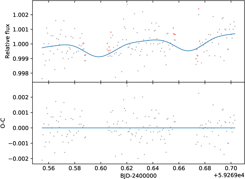
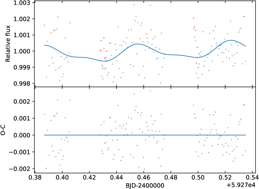
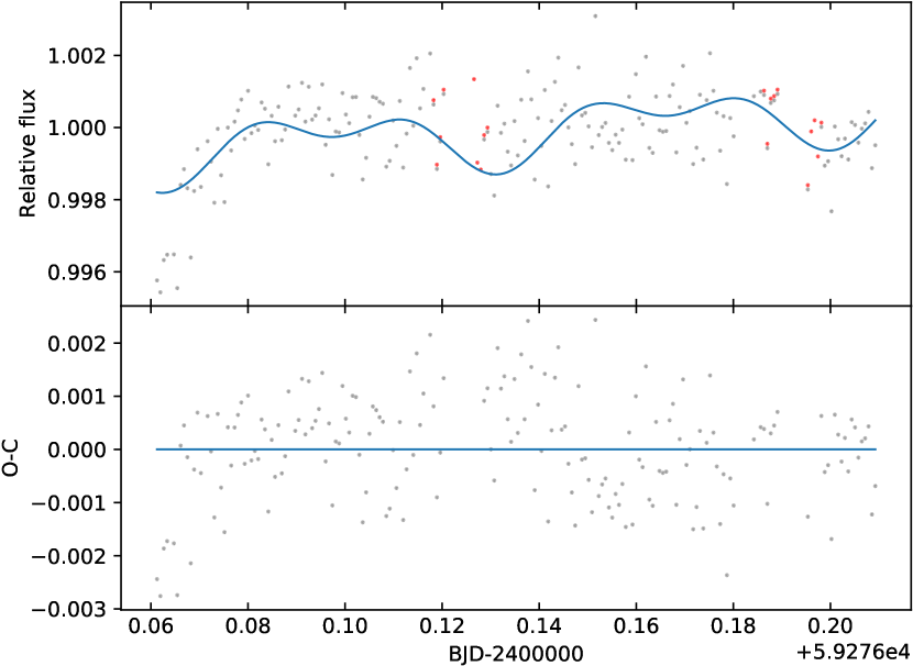
Figure 23: CHEOPS LCs and corresponding best fit for visits V1 to V3 from top to bottom respectively. For each panel, the top plot shows also the best fit model as a solid blue line, while the residuals are shown in the bottom plot. The red data points in the top panel show the rejected data. See Sect. 4.2 for details.

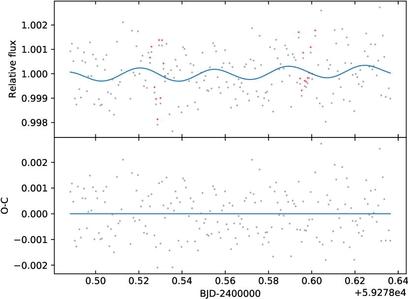
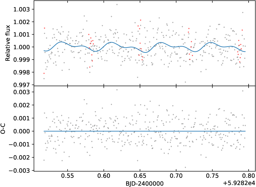
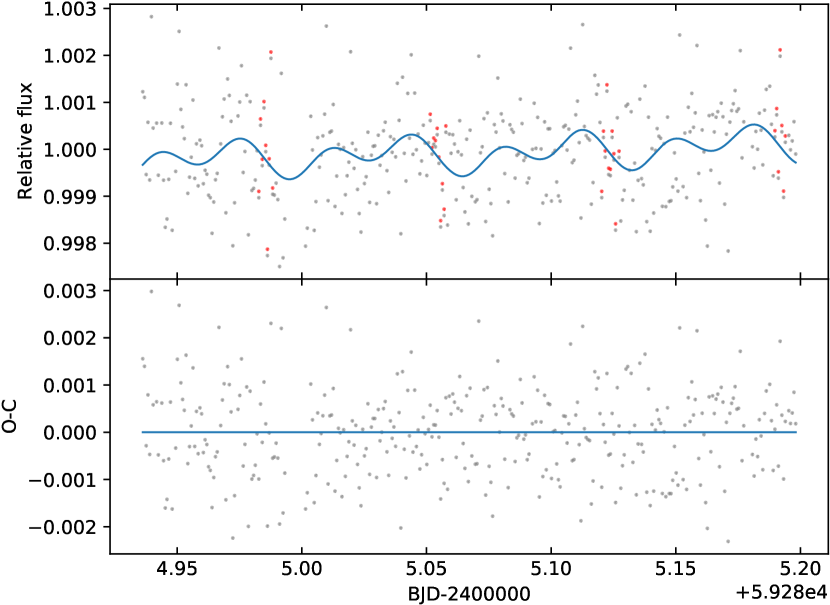
Figure 24: Same as in Fig. 23 for visits V4 to V6 from top to bottom respectively.

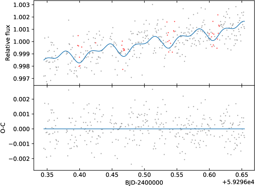
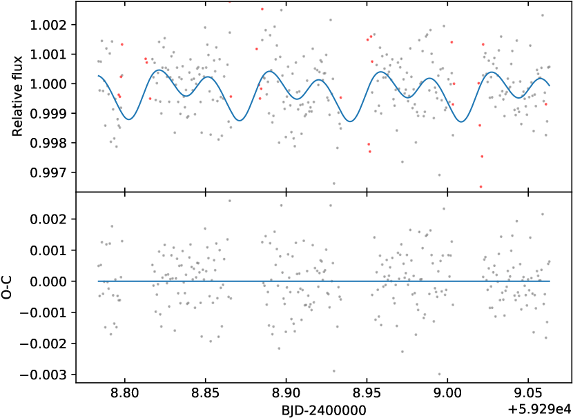
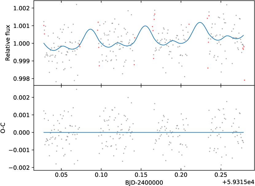
Figure 25: Same as in Fig. 23 for visits V7 to V9 from top to bottom respectively.

Finally, we normalized the LCs by the median value of the photometry. The final CHEOPS LCs are shown in Figs. 23–25 and publicly available at CDS.

2.2 TESS observations

TESS (Ricker et al. 2014) observed the WASP-43 system in sector 9 (from February,28 to March,26 2019, orbits 25 and 26) and in sector 35 (from February,9 to March,06 2021, orbits 77 and 78). Using the package lightkurve (Lightkurve Collaboration et al. 2018), we retrieved the 2 min cadence Simple Aperture Photometry (SAP) and Pre-search Data Conditioning Single Aperture Photometry (PDCSAP), which is corrected for instrumental systematics and for contamination from some nearby stars (Smith et al. 2012; Stumpe et al. 2012, 2014). We rejected all the data that are flagged by the pipeline. During sector 35 the telescope experienced a technical issue with the thermal stability and the pointing, which introduced trends and additional noise in the LC. To avoid these data, we also clipped out the photometry collected between BJD 2,459,255 and 2,459,256 and between BJD 2,459,266.2 and 2,459,272 (at the beginning and at the end of orbit 77).

For each orbit, we performed a preliminary normalization of the photometry by using the median value. The normalization will be refined in Sect. 4.1.

2.3 UVIS observations

Fraine et al. (2021) dedicated four HST orbits to observe a secondary eclipse of the WASP-43b system on 2019 July 3 using WFC3/UVIS with the F350LP filter in scanning mode. We retrieved the reduced photometry published by the authors and we kept the forward and reverse scan separated, so to detrend the two series independently. We did not apply any extra manipulation to the data.

2.4 Spectroscopic observations

We searched public archives for high resolution spectroscopic data for WASP-43. We ended up using three exposures observed with the Ultraviolet and Visual Echelle Spectrograph (UVES) which are public in the ESO archive and were taken under the program 090.C-0146. The instrumental configuration was Red Arm $@$580nm with a slit of 0.3”, which provided a coverage 472–683 nm with a resolution of $R=107200$. The exposure time was 691 s for each spectrum. The individual SNR is $\sim$40, while the SNR of the combined spectrum is $\sim$70.

3 Characterization of the host star

To determine the stellar parameters, we used the astroARIADNE package (Acton et al. 2020), a recent code that automatically retrieves photometric data (when existing) from catalogs such as ALL-WISE, APASS, Pan-STARRS1, SDSS, 2MASS and Tycho-2. With distances from Gaia, as well as available maps of dust distribution, the photometric data is fitted to different stellar models using Bayesian Model Averaging in order to find the best model of the stellar parameters. With this method we obtained T_eff=$4240^{+30}_{-20}$ K, $\log$(g)=4.71$\pm$0.09 cgs, [Fe/H]=$0.15^{+0.10}_{-0.04}$ dex, d=87.2$\pm$0.5 pc and $A_{\rm V}=0.05^{+0.04}_{-0.02}$, where the errors are internal to the statistical calculations.

We also used the IDL package Spectroscopy Made Easy (SME) to synthesize models of the observed spectrum. SME tests several atmospheric models (Valenti & Piskunov 1996; Piskunov & Valenti 2017), choosing eventually the one best agreeing with the observations. The code utilizes atomic and molecular line lists from VALD (Piskunov et al. 1995). In the case of WASP-43 we found that the model best agreeing with the observed spectrum are the MARCS 2012 models (Gustafsson et al. 2008) (Fig. 1). While keeping the turbulent velocities $V_{\rm mac}$ and $V_{\rm mic}$ fixed at values from Gray (2008), we determined the $v\sin i_{\star}$ =3$\pm$1 km s^-1, while the other derived spectroscopic parameters have larger uncertainties than the previously determined ones, which are thus preferred.

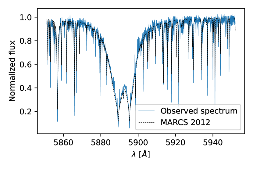
Figure 1: Comparison between the spectrum used for the stellar characterization around the Na i D_1,2 doublet and its bestfit model.

To compute the radius of WASP-43, we used a Markov-Chain Monte Carlo (MCMC) modified infrared flux method (IRFM; Blackwell & Shallis 1977; Schanche et al. 2020). By building spectral energy distributions (SEDs) from stellar atmospheric models and stellar parameters derived via our spectral analysis, we compared the determined synthetic fluxes to observed broadband photometry to calculate the apparent bolometric flux, and hence the stellar angular diameter and effective temperature. For WASP-43, we retrieved data taken from the most recent data releases for the following bandpasses; Gaia G, G_BP, and G_RP, 2MASS J, H, and K, and WISE W1 and W2 (Skrutskie et al. 2006; Wright et al. 2010; Gaia Collaboration et al. 2021) and used stellar atmospheric models from the atlas Catalogues (Castelli & Kurucz 2003). We converted our stellar angular diameter to the stellar radius using the offset-corrected Gaia EDR3 parallax (Lindegren et al. 2021) and obtained $R_{\star}=0.698\pm 0.014\,R_{\odot}$.

To compute the stellar mass $M_{\star}$ and age $t_{\star}$ we used two different stellar evolutionary models adopting the stellar effective temperature $T_{\mathrm{eff}}$, metallicity [Fe/H], and radius $R_{\star}$ as the basic input set. In detail, we applied the isochrone placement technique (Bonfanti et al. 2015, 2016) to pre-computed grids of PARSEC v1.2S (Marigo et al. 2017) isochrones and tracks to retrieve a first pair of mass and age estimates $(M_{\star,1};t_{\star,1})$. During interpolation, the basic input set was complemented with our internal estimate of $v\sin i_{\star}$ and with the stellar rotation period from Bonomo et al. (2017) in order to improve the fitting process convergence as described in Bonfanti et al. (2016). We obtained $M_{\star,1}=0.701\pm 0.030\,M_{\odot}$ and $t_{\star,1}=6.0\pm 3.9$ Gyr.

We determined a second pair of mass and age estimates $(M_{\star,2};t_{\star,2})$ using the CLES (Code Liègeois d’Évolution Stellaire, Scuflaire et al. 2008) code, which directly fits the basic input set within the Liège evolutionary models to retrieve the best-fit outcomes according to the Levenberg-Marquadt minimization scheme (Salmon et al. 2021). This on-the-fly computation yielded to $M_{\star,2}=0.728\pm 0.042\,M_{\odot}$ and $t_{\star,2}=10.1\pm 8.0$ Gyr.

As thoroughly described in Bonfanti et al. (2021), we finally merged the two respective pairs of age and mass values after carefully checking their mutual consistency through a $\chi^{2}$-based criterion and we obtained $M_{\star}=0.712_{-0.036}^{+0.041}\,M_{\odot}$ and $t_{\star}=7.4_{-5.3}^{+6.4}$ Gyr.

The characterization of WASP-43 is summarized in Table 2. The estimated parameters are in general agreement within uncertainties with previous characterizations (Bonomo et al. 2017; Esposito et al. 2017; Stassun et al. 2019).

Table 2: Stellar and system parameters.

Parameter	Symbol	Units	Value	Ref.
Spectral Type			K7V	Hellier et al. (2011)
Effective temperature	$\rm T_{eff}$	K	$4240^{+30}_{-20}$	this work
Surface gravity	$\log g$	$\log{\mathrm{cm/s^{2}}}$	$4.71\pm 0.09$	this work
Metallicity	[Fe/H]	—	$0.15^{+0.10}_{-0.04}$	this work
Distance	$d$	pc	$87.2\pm 0.5$	this work
Interstellar extinction	$A_{\rm V}$	—	0.05${}^{+0.04}_{-0.02}$	this work
Projected rotational velocity	$v\sin i_{\star}$	km/s	$3\pm 1$	this work
Stellar rotation period	$P_{\mathrm{rot}}$	d	$15.6\pm 0.4$	Hellier et al. (2011)
Stellar radius	$\rm R_{\star}$	$\rm R_{\sun}$	$0.698\pm 0.014$	this work
Stellar mass	$\rm M_{\star}$	$\rm M_{\sun}$	$0.712_{-0.036}^{+0.041}$	this work
Stellar age	$t_{\star}$	Gyr	$7.4_{-5.3}^{+6.4}$	this work
Radial velocity semi-amplitude	$\rm K_{RV}$	m/s	$551.5\pm 4.7$	Bonomo et al. (2017)

4 Light curve fitting

To fit the LCs we adopted the same model $F(\phi)$ as Esteves et al. (2013) (see also references therein), that is the sum of the transit model $F_{\rm tr}(\phi)$, the eclipse model $F_{\rm ecl}(\phi)$, the planet’s phase curve $F_{p}(\phi)$, the Doppler boosting of the stellar flux $F_{\rm d}(\phi)$ and the stellar ellipsoidal variations $F_{\rm e}(\phi)$:

$$F(\phi)=F_{\rm tr}(\phi)+F_{\rm ecl}(\phi)+F_{\rm p}(\phi)+F_{\rm d}(\phi)+F_{\rm e}(\phi),$$ (1)

where $\phi$ is the planet’s orbital phase. We do not go into the mathematical details of these terms (we refer the reader to Esteves et al. 2013; Singh et al. 2022, and references therein), but we give only a brief description and the list of parameters that define each of them.

To model the transits in the LC, we used the quadratic limb darkening (LD) law indicated by Mandel & Agol (2002) with the reparametrization of the LD coefficients suggested by Kipping (2013). We also assumed that the orbit of WASP-43b is circular following Hellier et al. (2011); Gillon et al. (2012); Bonomo et al. (2017). Under this hypothesis, the model $F_{\rm tr}(\phi)$ thus depends on the time of transit $\rm T_{0}$, the orbital frequency $\nu_{\rm orb}$ (the inverse of the orbital period $P_{\rm orb}$), the stellar density $\rho_{\star}$, the ratio between the planetary and stellar radii $R_{\rm p}/R_{\star}$, the impact parameter $b$ and the reparametrized quadratic LD coefficients $q_{1}$ and $q_{2}$. Also the eclipse model $F_{\rm ecl}(\phi)$ is formalized following Mandel & Agol (2002), but assuming that the planetary dayside hiding behind the stellar disc is uniformly bright.

The phase curve $F_{\rm p}(\phi)$ quantifies the amount of light that the planet emits towards the observer, either by reflection of the incoming stellar light or by thermal emission. In the hypothesis that the planet’s surface follows Lambert’s reflection law, the phase curve depends on the impact parameter $b$ and the amplitude of the phase curve $A_{\rm p}$ relative to the stellar flux. We also allowed the phase curve to peak at an offset $\Delta\phi$ from the eclipse center ($\phi$=0.5) in order to model any longitudinal asymmetry of the planet’s brightness.

In principle, $F_{\rm p}(\phi)$ should also account for the planetary thermal emission, both from the dayside and the nightside. For the planetary dayside, the shape of the thermal emission phase curves depend on how light is emitted by the planetary surface. Regardless of the level of anisotropy in the thermal emission and scattering, the thermal and reflected components have in common that they peak at or near secondary eclipse and smoothly decrease as the planet is closer to transit. For the thermal component, we estimated the dayside temperature of WASP-43b of $\sim 1600\leavevmode\nobreak\ K$ using the formalism in Cowan & Agol (2011), the orbital parameters provided by Esposito et al. (2017), the Bond albedo $A_{\rm B}$=0.19 and the recirculation efficiency $\epsilon$=0 estimated by Stevenson et al. (2017). If we approximate the planet and the star as black bodies, this dayside temperature translates into a planet-to-star contrast $A_{\rm day}=38$ ppm in the TESS band and 19 ppm in the HST WFC3/UVIS and CHEOPS bands. If we also assume that the dayside of WASP-43b reflects as a Lambertian surface, then the geometric albedo is expected to be A_g$\sim$0.13, which translates into a planet-to-star flux ratio of $A_{\rm refl}\sim$140 ppm, that is 7 times larger than the contrast of the planetary thermal radiation. The thermal phase curve of the planetary dayside thus provides a small contribution to the Lambertian phase curve, and the quality of the data analyzed in this paper does not allow to appreciate such small deviations from the reflection-only scenario. Thus, to reduce the number of free parameters, we fixed $A_{\rm day}=0$ letting the Lambertian phase curve absorb the thermal emission signal. In Sect. 5.4 we will discuss our findings on thermal emission and reflection from the planetary dayside.

As for the nightside, it has already been reported in the literature (Schwartz & Cowan 2015; Stevenson et al. 2017; Irwin et al. 2020) that the temperature is expected to be $\lesssim$1000 K, which corresponds to a negligible flux contrast of less than 1 ppm compared with the stellar flux. By consequence, in our data modeling we also excluded any nightside emission.

The Doppler boosting $F_{d}(\phi)$ is the modulation of the stellar flux due to the radial velocity of the star with respect to the observer. The observed flux increases when the star is moving towards the observer and decreases when it is moving away. This effect is thus phased with the orbital motion of the planet and depends on the radial velocity semi-amplitude $K_{\rm RV}$ and on the bandpass-integrated average spectral index $\alpha_{d}$ of the star.

The ellipsoidal variations are periodic modulations in the stellar light due to fluctuations in the shape of the stellar visible hemisphere, distorted by the tidal pull from the planet. $F_{e}(\phi)$ thus depends on the planet-to-star mass ratio $\mu$ (which is a function of $K_{\rm RV}$, $M_{\star}$ and the orbital parameters of the planet), the linear LD coefficient $u_{\rm LLD}$ and the gravity darkening coefficient $y_{\rm GD}$. As for the phase variations, the model also allows for an angular lag with respect to the planet’s orbital phase through the extra parameter $\Theta_{\rm lag}$.

The complete model thus depends on a total of 15 parameters. To reduce the dimensionality of the problem, and to avoid degeneracies which may occur among the model parameters, we locked some of them by means of prior knowledge coming from previous studies of the system. We fixed both $F_{d}(\phi)$ and $F_{e}(\phi)$ in Eq. 1 using the estimates of $K_{\rm RV}$ and $M_{\star}$ reported in Table 2. For the other input parameters, we proceeded as follows. We used the throughput of CHEOPS and TESS publicly available at the SVO Filter Profile Service (Rodrigo et al. 2012; Rodrigo & Solano 2020) and computed the passband-dependent $u_{\rm LLD}$ using the LDTk package . We computed $y_{\rm GD}$ in the TESS passband by a trilinear interpolation of the table provided by Claret (2017), assuming the stellar parameters listed in Table 2. Similarly, we performed the same computation using the table provided by Claret (2021) for the CHEOPS passband, using the gravity darkening exponent predicted by Claret (2000). For WFC3/UVIS we used similar tables that were provided in a private communication. We also fixed the spectral indices $\alpha_{d}$ (one for each instrument) by using the BT-Settl spectral model (Allard et al. 2012) with $\rm T_{eff}=4200\leavevmode\nobreak\ K$, $\log g=4.5$, $\rm[Fe/H]=0.3$ and no alpha elements enhancement. Finally, assuming that the tidal axis is aligned, we fixed $\Theta_{\rm lag}=0$. The expected amplitudes for the reflection phase curve, the thermal emission from the planetary dayside and nightside, the ellipsoidal variations and the Doppler boosting are summarized in Table 3.

Table 3: Expected amplitudes in ppm for the components in the LC model in the HST WFC3/UVIS, CHEOPS and TESS passbands.

	WFC3/UVIS	CHEOPS	TESS
Dayside thermal emission	19	19	38
Nightside thermal emission	0	0	0
Ellipsoidal variations	48	48	43
Doppler boosting	8	8	8

Another important point to take care of is the presence in the LCs of instrumental and/or stellar activity signals, which must be corrected in order to improve the quality of the LC modeling. The strategy to adopt depends on the characteristics of the datasets and is discussed separately for each instrument.

4.1 TESS light curves

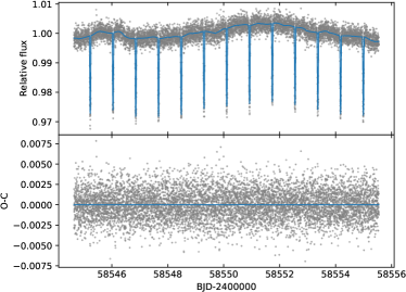
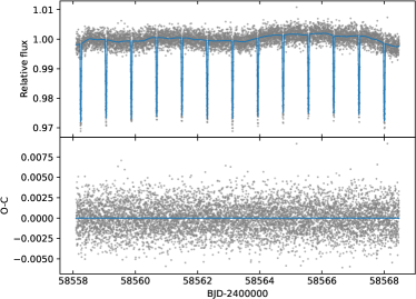
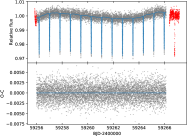
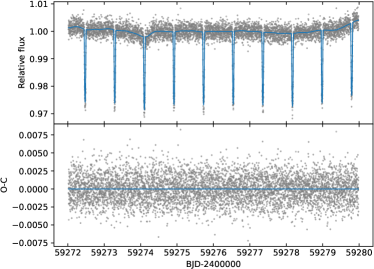
Figure 13: TESS LCs for orbits 25 (top left), 26 (top right), 77 (bottom left) and 78 (bottom right). For each panel, the top plot shows also the best fit model as a solid blue line, while the residuals are shown in the bottom plot. In the top plot of the bottom left panel we show in red the data rejected points. See Sect. 4.1 for details.

The TESS PDCSAP photometry is shown in Fig.13. It is clear that it is affected by red noise in the form of waves all along the LCs. We identified two possible origins for the trends. The first possibility is that they are artificially introduced by the detrending algorithm in the official reduction pipeline of TESS, as already claimed in previous works (for example Shporer et al. 2019; Wong et al. 2020a; Daylan et al. 2021). As a sanity check, since the correlated noise in the LCs seems to be periodic, for each sector we analyzed the Generalized Lomb Scargle Periodogram (Zechmeister & Kürster 2009) of both the SAP and PDCSAP photometry, after removing the transits. We found that all the periodograms look alike (Fig.2): they show a significant peak ( FAP¡0.1%) at $\sim 12.5$ d and its first harmonic ($\sim 6.3$ d, FAP¡0.1%) for both SAP and PDCSAP photometry. For sector 9 we also found a peak near 4 d, which corresponds to second harmonic of the 12.5 d period, while for sector 35 there is a peak near 3 d that is the fourth harmonic. We thus postulate that the detrending of the LCs is not the origin of the correlated noise in the data: if it is an artificial signal, then it must be already in the raw photometry, and not related to background or spacecraft jitter as that would have been cleaned up by the PDCSAP. Nonetheless, it is unlikely that the two light curves, obtained two years apart, are affected by instrumental issues leading to similar periodograms.

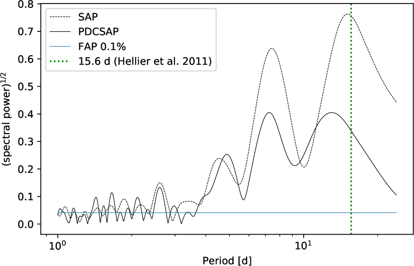
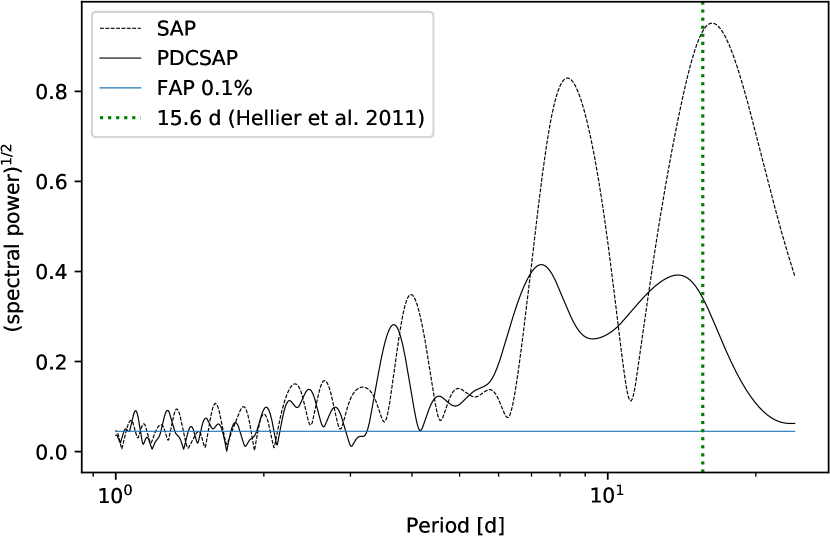
Figure 2: Periodogram of the TESS photometry (SAP and PDCSAP) of WASP-43, sectors 9 and 35 from top to bottom. In each panel, the vertical dashed line marks the 15.6 days rotation period proposed by Hellier et al. (2011).

Therefore, the second possibility is that the red noise is of stellar origin. As a matter of fact, if active regions are present on the stellar surface, then the stellar rotation typically introduces some periodic-like signals in the LCs, which can be identified by means of periodogram analysis. The stellar rotation has already been detected by Hellier et al. (2011), who claim a rotation period of $15.6\pm 0.4$ d with a photometric amplitude of 0.006 mag. Nonetheless, this rotation period does not seem a good match for the peaks in the periodograms of the TESS data. One possibility is that, due to differential rotation, we recovered a rotation period slightly shorter than what is indicated by Hellier et al. (2011). Moreover, if differential rotation and migration of active latitudes are in place, it is unlikely that we found the same rotation period in sectors which are two years apart.

Based on the discussion above, we are left with the ambiguity that the correlated noise in the LCs is of stellar origin or just instrumental effects not correctly removed, or maybe a combination of the two. Regardless of the source of the trends, we modeled them as a Gaussian Process (GP, Rasmussen & Williams 2006; Gibson et al. 2012) with a Matérn 3/2 kernel, that quantifies the covariance between two observations at times $t_{i_{1}}$ and $t_{i_{2}}$ as:

$$k(t_{i_{1}},t_{i_{2}})=h^{2}\left(1+\frac{\sqrt{3}|t_{i_{1}}-t_{i_{2}}|}{\rho}\right)\exp\left(-\frac{\sqrt{3}|t_{i_{1}}-t_{i_{2}}|}{\lambda}\right)+j_{o}^{2}\delta_{i_{1},i_{2}},$$ (2)

where $h$ is the amplitude of the GP and $\lambda$ is its timescale. In order to take into account any additional white noise, either instrumental or astrophysical, not included in the uncertainties, we added the diagonal elements $j_{o}^{2}\delta_{i_{1},i_{2}}$ where $o$ denotes the TESS orbit 25, 26, 77 and 78.

To trace any long-term activity signal, we also included in the model a linear function of time $t$ for each TESS orbit:

$$l_{o}(t)=c_{0,o}+c_{1,o}\cdot(t-t_{m,o}),$$ (3)

where the subscript $o$ denotes again the orbit of interest, while $t_{m,o}$ is the mid-time ($(t_{max}+t_{min})/2$) of the corresponding orbit $o$. With this representation, it is straightforward that the constant term refines the normalization of the LC, while the linear term traces any slope in the data.

We fit the data by maximizing in the parameter space the log-likelihood function given by:

$$\ln L=-\frac{n}{2}\ln(2\pi)-\frac{1}{2}\ln(\det{\bf K})-\frac{1}{2}{\bf\overline{r}^{T}}\cdot{\bf K}\cdot{\bf\overline{r}},$$ (4)

where $\overline{\bf r}$ is the array of length $n$ containing the residuals with respect to the model, while $\bf K$ is the covariance matrix obtained with the kernel in Eq. 2.

For the log-likelihood maximization we used a home made code written in the Python3 language. Our code reads in the prior distributions, one for each free parameter in the model, which define the boundaries of the parameter space within which the maximum likelihood location is searched for (Table 4). Then, using the python package PyDE, the code searches for the maximum likelihood location, which is used to initialize the MonteCarlo fit. Finally the algorithm samples the posterior probability distribution of the model parameters in a MCMC framework using the emcee package version 3.0.2 (Foreman-Mackey et al. 2013). The GP is implemented by using the celerite2 package version 0.0.2 (Foreman-Mackey et al. 2017; Foreman-Mackey 2018). Given the complexity and the demand of resources of the model fitting, we ran the code in the HOTCAT computing infrastructure (Bertocco et al. 2020; Taffoni et al. 2020).

Our Monte Carlo fit consisted of 100,000 steps, which corresponded to $\sim$300 times the auto-correlation length of the chains, estimated following Goodman & Weare (2010). This suggests that the fit successfully converged. We did not find any evidence of a linear long term trend in the data, thus we fixed $c_{1,o}=0$ in Eq. 3 for each of the four TESS orbits. The final list of free parameters, together with the corresponding priors, confidence intervals (C.I.) and Maximum A Posteriori (MAP) values, is reported in Table 4, while the posterior distributions are shown in Figs. 11–12. The best fit of the data is shown in Fig.13, while in Fig. 3 we show the data corrected for stellar activity and phase folded to the best fit orbital period. Our orbital solution is in general agreement with what is present in literature (Hellier et al. 2011; Bonomo et al. 2017; Esposito et al. 2017).

To test the robustness of our findings, we also tried other simplified models by assuming iteratively a flat out-of-transit LC, a phase curve with no reflection component from the planet, a model with no ellipsoidal variation or doppler boosting and a complete phase curve with no phase offset in the reflection component. We compared all the models using the Akaike Information Criterion (AIC, Burnham & Anderson 2002). We found that the most likely model is the one described so far, while the second model ranked by the AIC is the one with $\Delta\phi=0$, with a relative likelihood of 14%. The AIC and 2-$\sigma$ detection on $\Delta\phi$ in Table 4 thus make the detection of the phase offset only marginal. All the other models have likelihood $<2\%$ and therefore we omit them from further consideration.

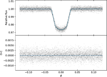
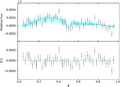
Figure 3: Left - Close-up of the phase folded planetary transits observed with TESS, after the removal of the stellar activity (top panel). The solid blue line is the best fit model, while the black dots represent the rebinned photometry. The corresponding residuals are shown in the bottom panel. Right - Same as in the left panel, but centered on the eclipse. For visualization purposes, the vertical axis has been zoomed in and only the rebinned photometry is shown. To give an idea of the uncertainty on the best fit model, the shaded cyan lines in the top panel correspond to the model computed using 100 random steps in the MCMC chain.

Table 4: Model parameters for the fit of the TESS data.

Jump parameters	Symbol	Units	MAP	C.I.	Prior
GP amplitude	$\log h$	—	-6.6	-6.5(1)	$U$(-7,-3)
GP timescale	$\log\frac{\lambda}{\rm 1\leavevmode\nobreak\ day}$	—	-0.3	-0.3(1)	$U$(-8,4)
Time of transit	$T_{0}$	BJDTDB-2400000	58912.10729	58912.10729(3)	$U$(58912.1071,58912.1075)
Orbital frequency	$\nu_{\rm orb}$	days-1	1.2292955	1.2292955(1)	$U$(1.229295,1.229296)
Stellar density	$\rho_{\star}$	$\rho_{\sun}$	2.20	2.20(4)	$U$(2,2.5)
Radii ratio	$R_{p}/R_{\star}$	—	0.1597	0.1597(4)	$U$(0.154,0.165)
Impact parameter	b	—	0.684	0.684(7)	$U$(0.64,0.73)
First LD coef.	q1	—	0.39	0.39(2)	$N$(0.454,0.013)
Second LD coef.	q2	—	0.39	0.39(2)	$N$(0.401,0.024)
Phase curve amplitude	Ap	ppm	180	160(60)	$U$(0,300)
Phase offset	$\Delta\phi$	—	0.14	$0.13^{+0.06}_{-0.08}$	$U$(-0.2,.5)
Jitter in orbit 25	jo25	ppm	0	$90^{+80}_{-60}$	$U$(0,2000)
Normalization of orbit 25	c0,o25	—	-0.0001	-0.0001(6)	$U$(-0.02,0.02)
Jitter in orbit 26	jo26	ppm	0	$100^{+100}_{-70}$	$U$(0,2000)
Normalization of orbit 26	c0,o26	—	-0.0002	-0.0002(6)	$U$(-0.02,0.02)
Jitter in orbit 77	jo77	ppm	0	$80^{+80}_{-60}$	$U$(0,2000)
Normalization of orbit 77	c0,o77	—	0.0002	0.0002(6)	$U$(-0.02,0.02)
Jitter in orbit 78	jo78	ppm	400	$370^{+80}_{-100}$	$U$(0,2000)
Normalization of orbit 78	c0,o78	—	0.0005	0.0005(6)	$U$(-0.02,0.02)
Fixed parameters	Symbol	Units	Value		Notes
Linear trend for orbit 25	c1,o25	days-1	0
Linear trend for orbit 26	c1,o26	days-1	0
Linear trend for orbit 77	c1,o77	days-1	0
Linear trend for orbit 78	c1,o78	days-1	0
Stellar mass	M⋆	M☉	0.71		see Table 2
RV semi-amplitude	KRV	m/s	551.7		see Table 2
Linear LD coef.	uLLD	—	0.548		computed with LDTk
GD coef.	yGD	—	0.426		from Claret (2017)
Tidal lag	$\Theta$	rad	0
Derived parameters	Symbol	Units	MAP	C.I.	Notes
Planetary radius	$R_{\rm p}$	$R_{\rm J}$	1.08	1.08(2)
Orbital period	Porb	day	0.81347406	0.81347406(7)
Transit duration	T14	hr	1.242	1.242(4)
Scaled semi-major axis	$a/R_{\star}$	—	4.77	4.77(3)
Orbital inclination	$i$	degrees	81.8	81.8(1)
Eclipse depth	$\delta_{\rm ecl}$	ppm	120	110(50)	260 (99.9% upper limit)

4.2 CHEOPS light curves

We analyzed the CHEOPS LCs using the same Monte Carlo framework described in Sect. 4.1, taking into account the fact that the visits last only a few hours around the secondary eclipses of WASP-43b. Thus, the dataset does not allow the reconstruction of the full phase curve, but only the flux drop during the eclipse. Moreover, given the eclipse depth measured in the TESS band (Sect. 4.1), we did not expect the eclipse signal in the CHEOPS LCs to be strong enough to constrain the ephemeris of the system. For these reasons we fixed the orbital parameters and $\rho_{\star}$ to their MAP values in Table 4. We also fixed $\Delta\phi=0$: this makes a perfect correspondence between the amplitude of the phase curve $A_{\rm p}$ and the eclipse depth $\delta_{\rm ecl}$.

Since the CHEOPS LCs are only a few hours long, much shorter than the stellar rotation period, the rotation signal cannot be modeled with a periodic function. We thus modeled the activity signal in each visit with a linear term of the form:

$$l_{v}(t)=c_{0,v}+c_{1,v}\cdot(t-t_{m,v}),$$ (5)

where the subscript $v$ indicates the CHEOPS visit ID from V1 to V9 (see Table 1), while $t_{m,v}$ is the mid-time of the corresponding visit $v$.

As discussed in previous analyses (e.g. Deline et al. 2022; Hooton et al. 2022; Wilson et al. 2022), CHEOPS photometry is affected by variable contamination from other stars in the field of view. The variability of this contamination is due to the fact that the Point Spread Function (PSF) of the stars is not circular, and the overlap with the target PSF depends on the roll angle of the telescope (Benz et al. 2021). Both the DRP and PIPE have a module that decontaminates the aperture used for the photometric extraction, but residual signals are present in the LCs due to inaccuracies in the correction. This spurious signal $\Phi$ is phased with the roll angle $\phi_{\rm CH}\in[0,2\pi]$ of the CHEOPS satellite, and changes from visit to visit. To remove this signal, we included in our algorithm a module which fits independently for each visit $v$ the harmonic expansions of a periodic signal up to the first five harmonics, the fundamental harmonic having period $\rm 2\pi$:

$$\Phi_{v}(\phi_{\rm CH})=\Sigma_{i=1}^{5}\left[a_{i,v}\sin(i\cdot\phi_{\rm CH})+b_{i,v}\cos(i\cdot\phi_{\rm CH})\right]$$ (6)

Finally, to take into account any white noise not included in the formal photometric uncertainties, we added to our model a diagonal GP kernel of the form:

$$k(t_{i_{1}},t_{i_{2}})=j_{v}^{2}\delta_{i_{1},i_{2}},$$ (7)

with an independent jitter term $j_{v}$ for each CHEOPS visit V1 to V9.

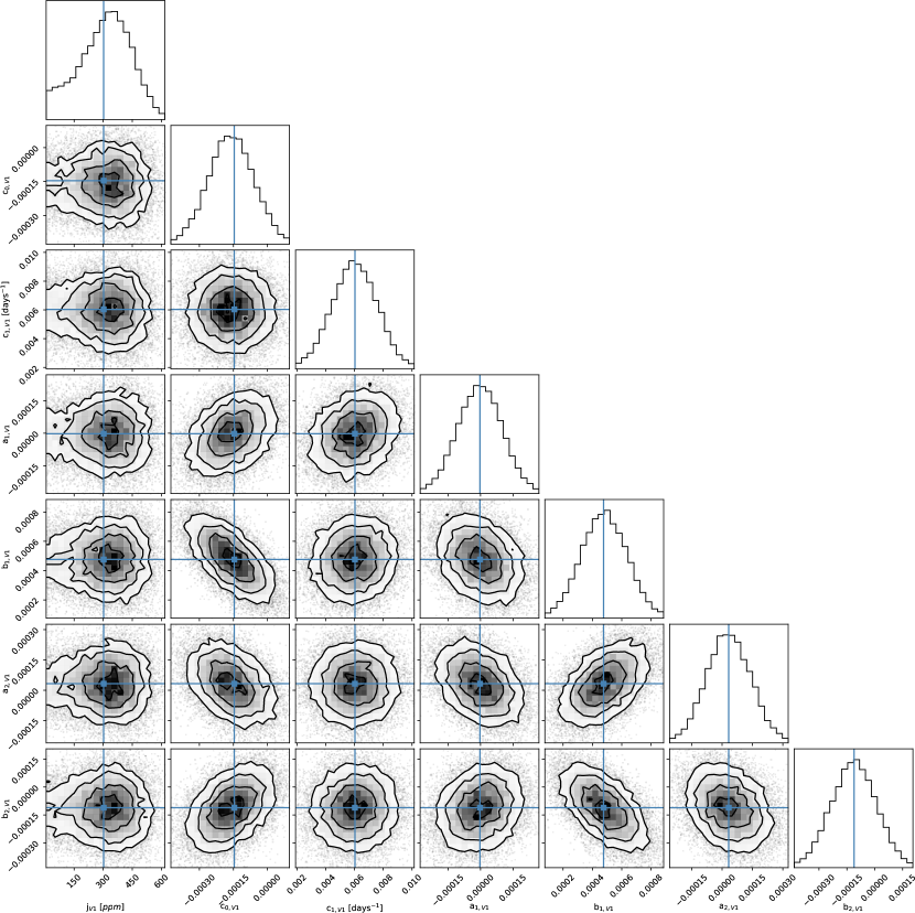
Figure 14: Corner plot of the MCMC chains of the jitter parameter, the linear trend coefficients and the instrumental decorrelation coefficients from the fit of the CHEOPS LCs (see Sect. 4.2). In each panel, the solid lines mark the MAP values. For plotting purposes, only the coefficients related to visit V1 are shown. The corner plots for the other visits are shown in the next figures. The posterior distribution of $A_{p}$ is not shown here as it corresponds to what shown in Fig. 8.

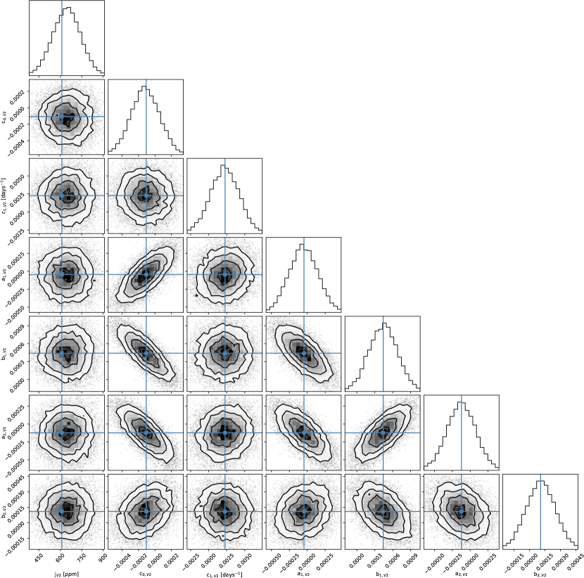
Figure 15: Same as in Fig. 14 for CHEOPS visit V2.

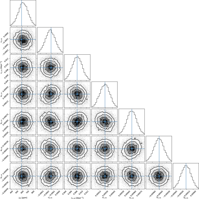
Figure 16: Same as in Fig. 14 for CHEOPS visit V3.

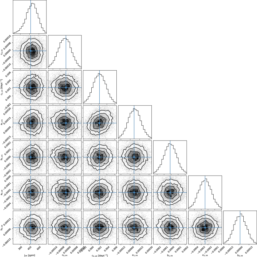
Figure 17: Same as in Fig. 14 for CHEOPS visit V4.

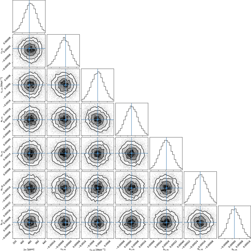
Figure 18: Same as in Fig. 14 for CHEOPS visit V5.

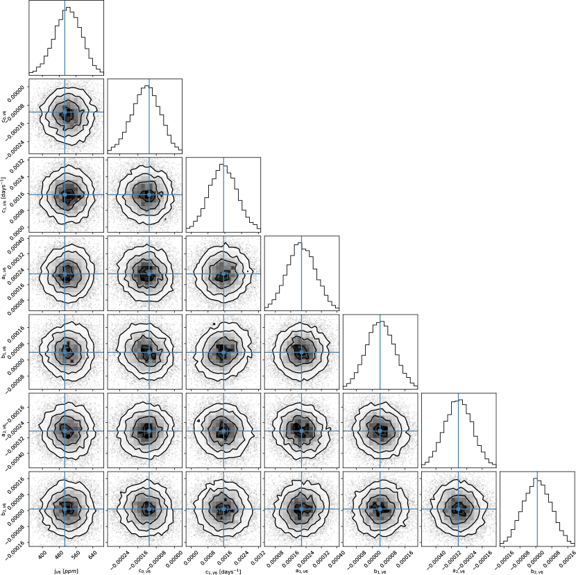
Figure 19: Same as in Fig. 14 for CHEOPS visit V6.

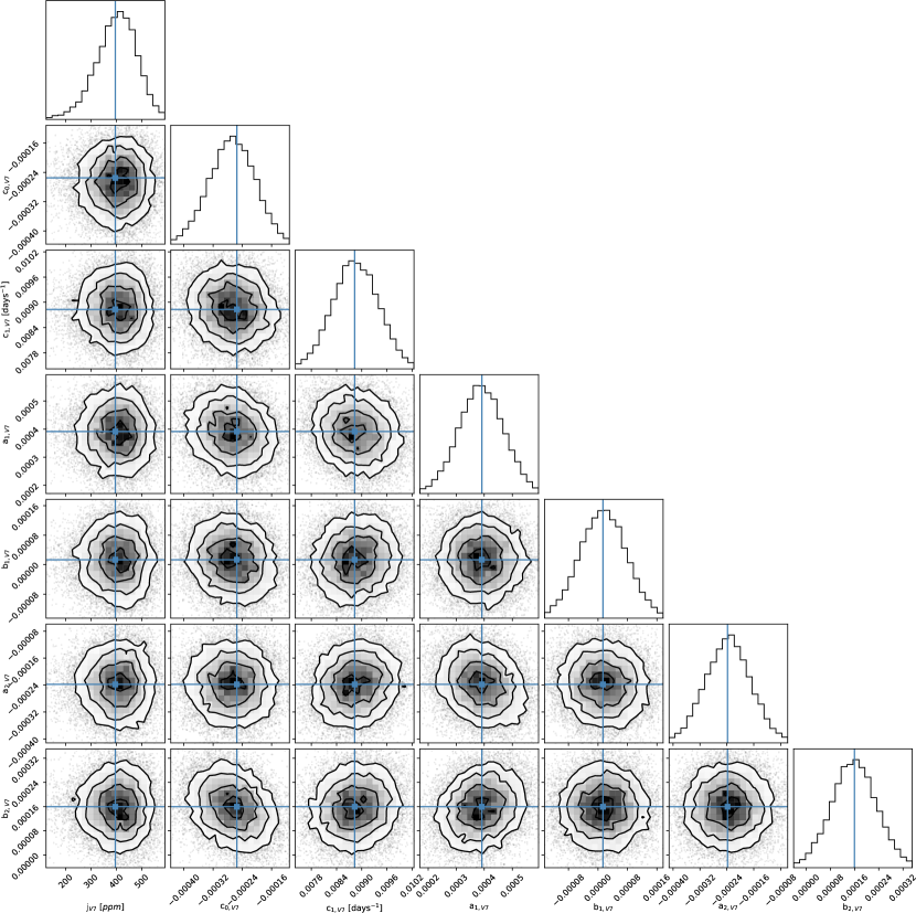
Figure 20: Same as in Fig. 14 for CHEOPS visit V7.

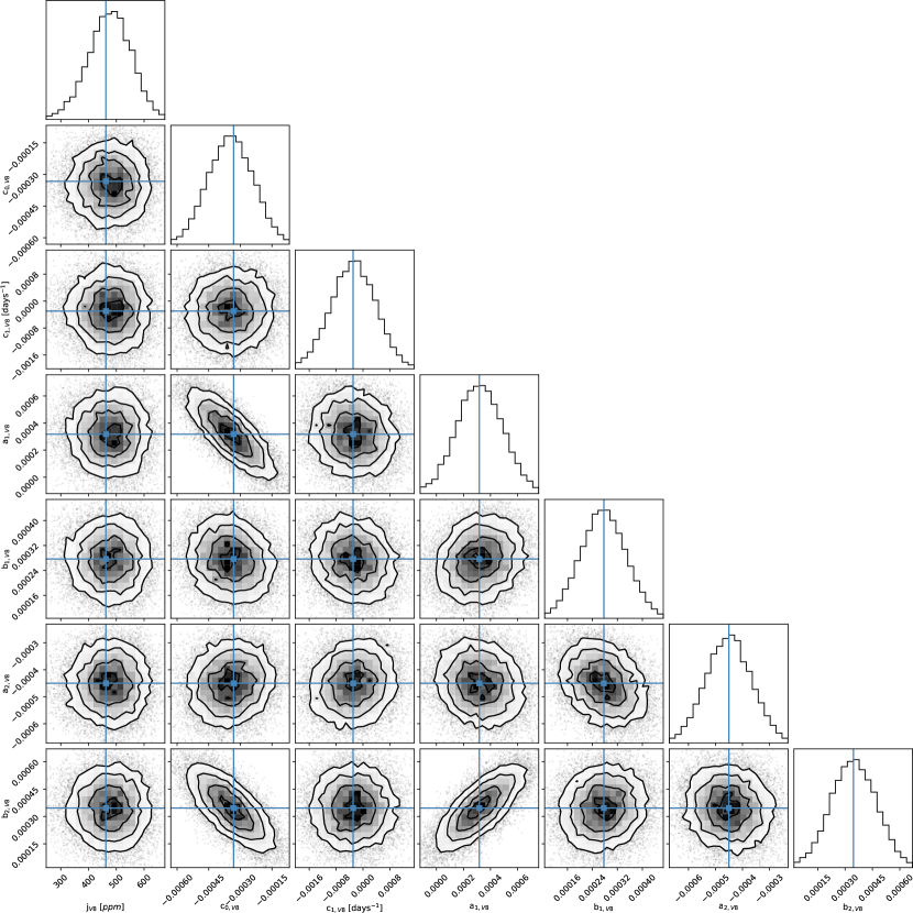
Figure 21: Same as in Fig. 14 for CHEOPS visit V8.

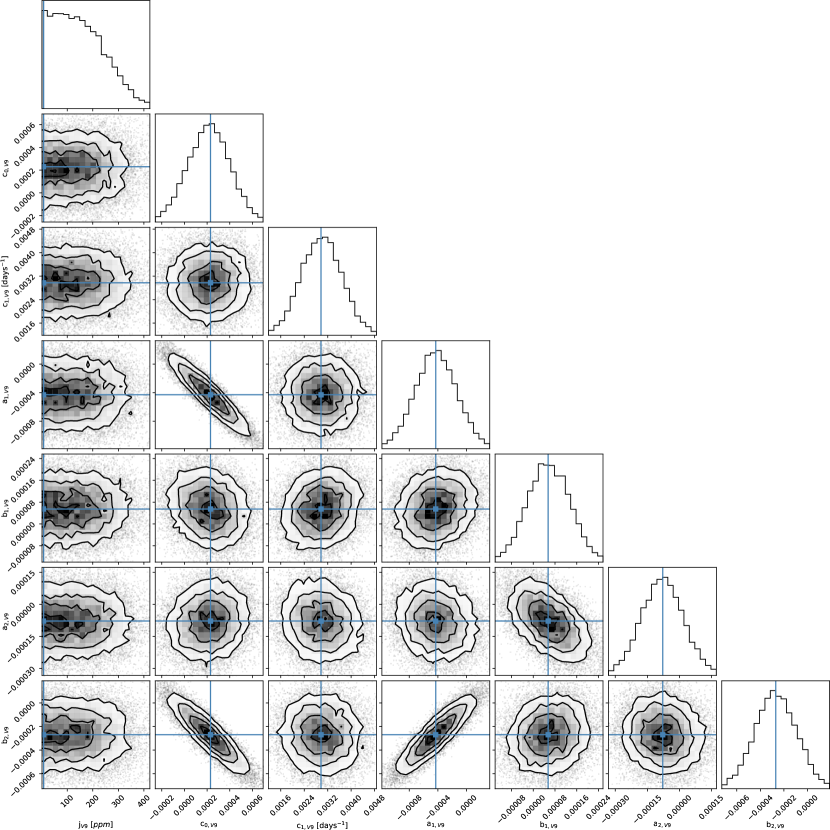
Figure 22: Same as in Fig. 14 for CHEOPS visit V9.

As for the fit of the TESS data, we searched the best-fit parameters by maximizing the likelihood expressed as in Eq. 4. We stopped the MonteCarlo fit after 100,000 steps ($\sim$60 times the autocorrelation time of the chains), so to expect that the chains are sufficiently converged. The fitted parameters, priors and posterior distributions are listed in Table LABEL:tab:CHEOPSfit and shown in Figs. 14-22. We remark that, not having any CHEOPS observation of the transits, the parameters $k$, $q_{1}$ and $q_{2}$ cannot be fitted. This explains why they are not listed in the table. The data corrected for correlated noise (instrumental and stellar) and phase folded to the orbital period are shown in Fig. 4 together with the best fit planetary model computed using the MAP parameters. The best fit of the individual CHEOPS visits is shown in Figs.23-25.

We also tried the same model discussed above with the reflected light component removed. This last model has a lower AIC and should thus be preferred. Nonetheless, the model including the planetary phase curve has a non negligible relative likelihood of $\sim$33%. Moreover, being a transiting system in a circular orbit, the eclipse signal must be in the data, as confirmed by the analysis of the TESS LCs (Sect. 4.1). We thus prefer the former, more complex model because it at least puts an upper limit to the eclipse depth in the CHEOPS passband.

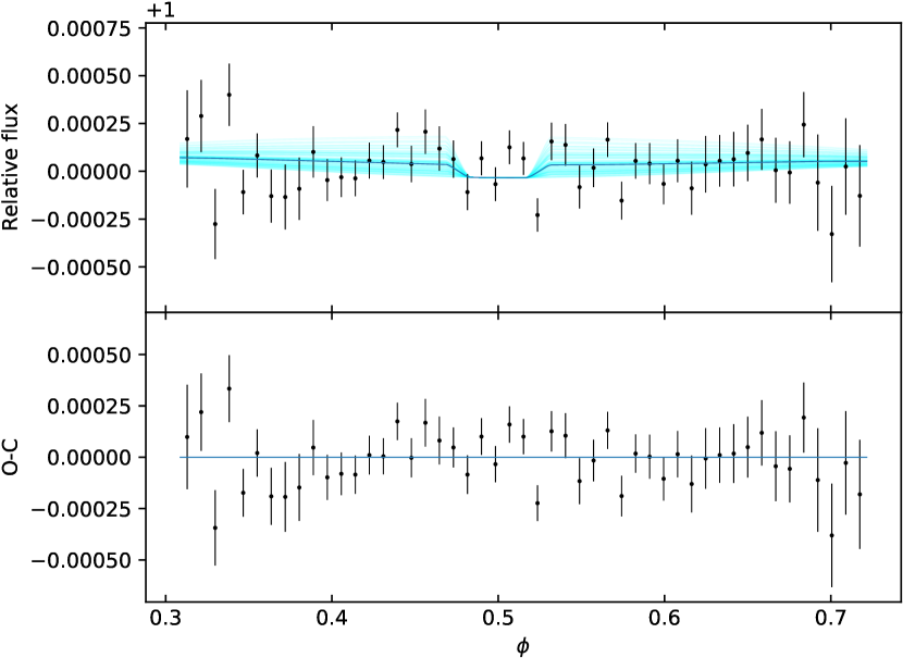
Figure 4: Phase folded CHEOPS photometry of the secondary eclipses of WASP-43b, corrected for stellar and instrumental correlated noise. The solid line is the best fit model. The corresponding residuals are shown in the bottom panel. For visualization purposes, in both panels the data are binned at regular steps. The shaded cyan lines in the top panel correspond to the model computed using 100 random steps in the MCMC chain.

4.3 UVIS light curves

Fraine et al. (2021) analyzed the HST WFC3/UVIS data using a simple box model and provide an upper limit to the eclipse depth. We re-analyzed the same data using a more realistic model (Sect. 4) and the most up to date ephemeris (Sect. 4.1).

The scheduling of the HST WFC3/UVIS observations was similar to the ones of CHEOPS, in the sense that the target has been followed up only for a few hours around a secondary eclipse. For what concerns the modeling of the secondary eclipses and the stellar activity, we thus adopted the same approach described in Sect. 4.2. The main difference is that we fit a linear trend independently for the forward and reverse scan

$$l_{s}(t)=c_{0,s}+c_{1,s}\cdot(t-t_{m,s}),$$ (8)

where $s$ indicates the scan direction (“F” for forward and “R” for reverse) and $t_{m,s}$ is the mid-time of the scan. The main purpose is to allow for different normalization coefficients depending on the scan direction.

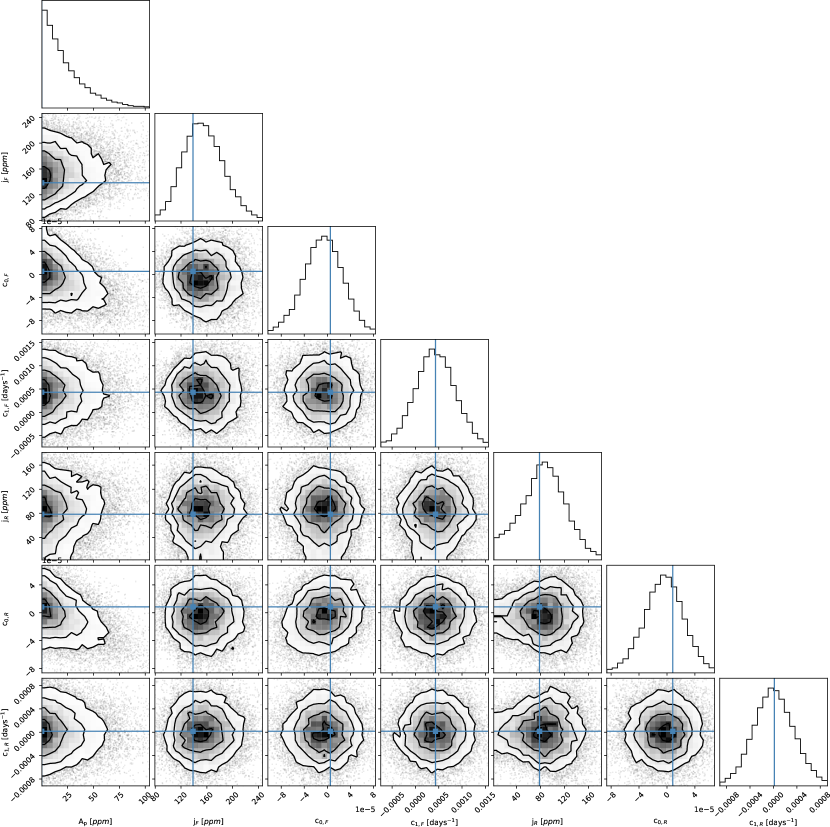
Figure 26: Corner plot of the MCMC chains from the fit of the HST WFC3/UVIS LCs (see Sect. 4.3). In each panel, the solid lines mark the MAP values. For plotting purposes, only the coefficients related to visit V1 are shown. The corner plots for the other visits are shown in the next figures. The posterior distribution of $A_{p}$ is not shown here as it corresponds to what shown in Fig. 8.

Using the same MonteCarlo framework as in Sect. 4.1 and Sect. 4.2, we ran 10,000 steps to ensure convergence. The outcome of the fit is listed in Table 5 and shown in Fig. 26. In Fig. 5 we plot the UVIS LCs together with the best fit model computed with the MAP values.

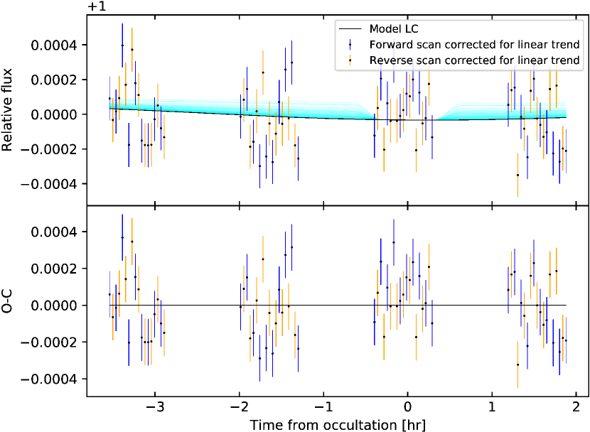
Figure 5: HST WFC3/UVIS photometry of WASP-43, corrected for stellar linear trends. The solid line is the best fit model. The corresponding residuals are shown in the bottom panel. The shaded cyan lines in the top panel show the model computed using 100 random steps in the MCMC chain.

Table 5: Model parameters for the fit of the HST WFC3/UVIS data.

Jump parameters	Symbol	Units	MAP	C.I.	Prior
Phase curve amplitude	Ap	ppm	0	$20^{+30}_{-10}$	$U$(0,500)
Jitter for forward scan	jF	ppm	140	150(30)	$U$(0,2000)
Normalization of forward scan	c0,F	—	0.00001	-0.00001(3)	$U$(-0.002,0.002)
Linear trend of forward scan	c1,F	days-1	0.0004	0.0004(4)	$U$(-0.03,0.03)
Jitter for reverse scan	jR	ppm	80	90(40)	$U$(0,2000)
Normalization of reverse scan	c0,R	—	0.00001	-0.00000(3)	$U$(-0.002,0.002)
Linear trend of reverse scan	c1,R	days-1	0	0.0000(3)	$U$(-0.03,0.03)
Fixed parameters	Symbol	Units	Value		Notes
Transit time	$T_{0}$	BJDTDB-2400000	58912.10729		see Table 4
Orbital frequency	$\nu_{b}$	days-1	1.2292955		see Table 4
Stellar density	$\rho_{\star}$	$\rho_{\sun}$	2.20		see Table 4
Stellar mass	M⋆	M☉	0.71		see Table 2
RV semi-amplitude	KRV	m/s	551.7		see Table 2
Linear LD coef.	uLLD	—	0.652		computed with LDTk
GD coef.	yGD	—	0.521		private communication
Phase offset	$\Delta\phi$	—	0
Tidal lag	$\Theta$	rad	0
Derived parameters	Symbol	Units	MAP	C.I.	Notes
Eclipse depth	$\delta_{\rm ecl}$	ppm	0	$20^{+30}_{-10}$	130 (99.9% upper limit)

5 Discussion

5.1 Stellar activity

In the model used to fit the TESS LCs we included a GP to detrend the data against the red noise, regardless of its origin. In the case that it is due to stellar activity, the amplitude of the GP ($\sim$1.5 mmag) is about 4 times lower than Hellier et al. (2011), thus suggesting a smaller photometric signal due to active regions. This can be due, first of all, to the fact that the TESS passband peaks at longer wavelengths, for which the contrast of active regions is lower. Another explanation is that TESS has observed WASP-43 in a less active state, or that the spot configuration during TESS observations was more uniform than during the WASP-South campaign. In any case, everything points to a scenario of a poorly variable star.

In the hypothesis that the red noise is periodic, as suggested by the periodograms in Fig. 2, we also tried the SHO kernel for the GP modeling, as it has been reported to be appropriate for periodic signals (Foreman-Mackey et al. 2017). Nonetheless, a posteriori we found that the SHO kernel is not able to catch the periodic-like correlated noise in the data. According to Serrano et al. (2018), the time span covered by the TESS sectors would be long enough to detect the  15 day rotation period, but two factors act against a clear detection. The first limitation comes from the small amplitude of the photometric variability. Secondly, the reconstruction of the periodic signal is hampered if the damping timescale of the kernel is shorter than the period of the GP, i.e. the activity signal evolves on timescales shorter than the rotation period. This partially washes out the periodicity of the rotation signal, which can thus no longer be accurately caught by the time-series analysis.

Given the definition in Eq. 2, the covariance of the Matérn 3/2 kernel is expected to decay by a factor of 10 after 1 d. This means that any signal with timescales shorter than 1 d can hardly be absorbed by the GP. As a matter of fact, the periodogram of the residuals in Fig.6 shows that at frequencies higher than $\sim 1\leavevmode\nobreak\ [d^{-1}]$ (periods shorter than 1 d) the power spectrum is consistent with white noise, while at shorter frequencies (longer periods) the periodogram drops by 3 orders of magnitude, the missing power being absorbed by the GP. This evidence has a twofold implication. First of all, since the GP absorbs power at period longer than 1 d, it is unlikely that it interferes with the phase curve, whose periodicity is $P_{\rm orb}=0.81347406\leavevmode\nobreak\ d$ (Table 4). Secondly, since the periodogram of the residuals does not show any significant deviation from white noise, we also conclude that there is no evidence of remaining correlated noise in the data, and that the posteriors of the MCMC fit are unbiased.

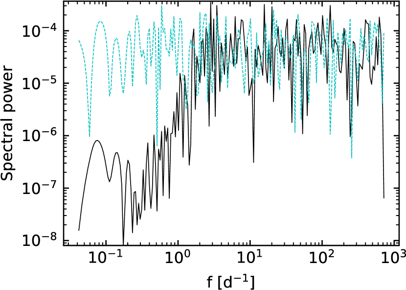
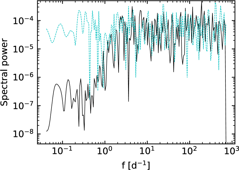
Figure 6: Periodogram of the residuals of the best fit of sector 9 (top panel) and sector 35 (bottom panel). In each panel, the cyan dashed line shows the periodogram of a randomly generated flat LC with the same time sampling and noise corresponding to the variance of the residuals of the fit.

To tackle the problem of correlated noise we also used the approach proposed by Pont et al. (2006): we analyzed how the standard error on the average $\sigma_{\rm n}$ scales with the sample size $n$ of residual data points in a time interval corresponding to the transit duration (Fig. 7, left panel) and to the orbital period (Fig. 7, right panel). In both cases, we found that $\sigma_{\rm n}$ scales down as $n^{1/2}$, which is expected in absence of red noise in the residual time series. We thus conclude that the model used to fit the data absorbs both the astrophysical signals and the correlated noise (astrophysical and instrumental), returning unbiased estimate of the planetary parameters. This is consistent with the fact that the jitter terms $j_{\rm o}$ in Eq. 2 are all consistent with 0. The only exception is TESS orbit 78, for which we postulate instrumental issue intervening between orbits 77 and 78.

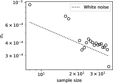
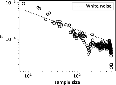
Figure 7: Scaling of the standard error of the average $\sigma_{\rm n}$ as a function of the sample size $n$. Left and right panels show respectively the empirical scaling relation for a time bin corresponding to the transit duration $T_{\rm 14}$=1.245 hr and the orbital period $P_{\rm orb}$=0.81347406 d (see Table 4). In each panel the dotted line shows the expected trend in the assumption of purely white noise.

Finally, searching for additional clues on stellar activity, we fit the two TESS sectors independently and we found that the corresponding $R_{\rm p}/R_{\star}$ ratios are consistent within uncertainties. This result indicates that, if active regions are present on the stellar surface, their overall configurations during the two sectors are similar.

5.2 Orbital parameters

The analysis of the TESS LCs allowed us to update the ephemeris and transit parameters of WASP-43b. Our determination of the orbital parameters agrees within 3$\sigma$ with previous ground-based studies (Hellier et al. 2011; Esposito et al. 2017; Wong et al. 2020b; Garai et al. 2021).

In particular, we do not find any significant discrepancy among our estimate of $R_{p}/R_{\star}$ and the ones reported in literature at previous epochs. This has a twofold implication. At the current photometric precision, the evolution of the activity signal is not significant enough to affect the planetary radius measurement, as it is the case, for example, for more active stars like CoRoT-2 (Czesla et al. 2009; Silva-Valio et al. 2010). This is consistent with the low activity scenario for WASP-43, as discussed previously. Moreover, comparing the measurements using different bandpasses, no significant trend with wavelength is detected. This implies that neither stellar activity nor the planetary atmosphere significantly affect the transmission spectrum in the optical domain.

5.3 Phase curve

The atmospheric phase curve of WASP-43b has been modeled with two free parameters: the amplitude $A_{\rm p}$ and the phase offset $\Delta\phi$. Using TESS data we obtained a $\sim 3\sigma$ detection for the amplitude $A_{\rm p}$ (160$\pm$60 ppm), while other data sets led to a marginal 2$\sigma$ detection (CHEOPS, $80^{+60}_{-50}$ ppm) or to an upper limit (HST WFC3/UVIS, $A_{\rm p}<130$ ppm).

The extended phase coverage of TESS data also allowed to investigate the presence of an offset in the atmospheric phase curve, leading to a marginal 2$\sigma$ detection of $\Delta\phi=0.13^{+0.06}_{-0.08}$, that corresponds to an eastward angular offset of $\left(50^{+30}_{-20}\right)^{\circ}$ with respect to the substellar point. This estimate, despite marginal, is consistent with the eastward offset of $21.1^{\circ}\pm 1.8^{\circ}$ detected by Stevenson et al. (2017) using Spitzer data.

Wong et al. (2020b) and Blažek et al. (2022) recently published independent extractions of the planetary phase curve from TESS LCs using different flavors of data detrending and modeling. Their results are consistent with ours and confirm the difficulty to reach a clear detection of the planetary emission signal using only TESS data, due to the faintness of the reflected light.

5.4 Geometric albedo

The eclipse depth $\delta_{\rm ecl}$ is a direct measurement of the flux contrast $F_{p}/F_{\star}$ between the planet and its parent star when the planetary disk is fully illuminated ($\phi=0.5$), and in principle incorporates the contribution from both the reflection of the stellar spectrum and the thermal emission from the planetary surface.

In our framework (Sect. 4) $\delta_{\rm ecl}$ is not a free parameter but a quantity derived from the phase curve model. This is particularly important for the fit of the TESS LCs, where we allowed for a free phase offset $\Delta\phi$. As a matter of fact, a non zero phase offset makes the eclipse depth smaller than the overall amplitude $A_{\rm p}$ of the phase curve. Aiming at a fully Bayesian analysis of the planetary albedo, for each couple ($A_{\rm p}$, $\Delta\phi$) sampled in the MCMC fit of the LCs we derived the corresponding $\delta_{\rm ecl}$. For the case of HST WFC3/UVIS and CHEOPS LCs, as we explain in Sect. 4.2, we artificially fixed the phase offset to zero, which led to exact correspondence with the amplitude of the phase curve $A_{\rm p}$. In Fig. 8 we show the distribution of the eclipse depths for the HST WFC3/UVIS, CHEOPS and TESS LCs respectively.

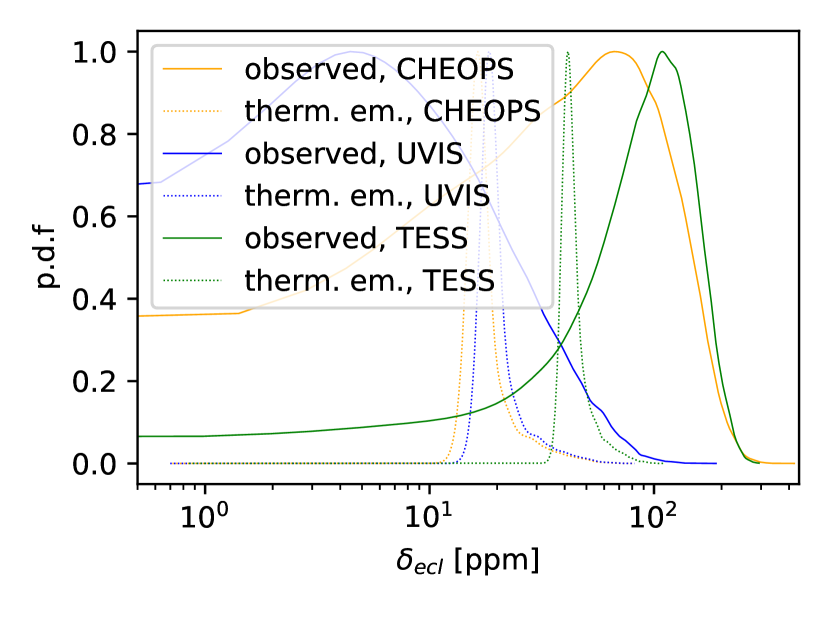
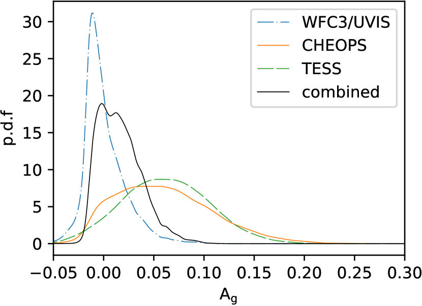
Figure 8: Top panel - Posterior distribution functions (PDF) of the thermal contamination (dotted lines) and measured eclipse depths $\delta_{\rm ecl}$ (solid lines) derived from the fit of the HST WFC3/UVIS, CHEOPS and TESS LCs. For clarity, each function has been rescaled so to peak at 1. Bottom panel - Normalized PDFs of the geometric albedo $A_{g}$ in the HST WFC3/UVIS, CHEOPS and TESS passbands. The combined PDF is shown as a black solid line.

In the case of reflection, the eclipse depth can be expressed as:

$$\delta_{\rm ecl}=\frac{F_{p}}{F_{\star}}=A_{g}\left(\frac{R_{p}}{a}\right)^{2},$$ (9)

where A_g is the planetary geometric albedo (Seager 2010). In this perspective, the eclipse depth is the observable directly linked the geometric albedo of the planet, but only if the thermal emission in the passband of interest can be either corrected or neglected.

To estimate the thermal emission in the HST WFC3/UVIS, CHEOPS and TESS passbands we employed the Helios-r2 Bayesian retrieval framework. This code was first introduced in Kitzmann et al. (2020) for studying emission spectra of brown dwarfs. It was upgraded in Wong et al. (2021) to perform retrievals of secondary eclipse observations as well. The forward model of Helios-r2 calculates the planet’s emission spectrum based on a number of free parameters and then converts the result into a secondary eclipse depth using a spectrum for the host star. Since some of the available observations are measured over wide bandpasses, Helios-r2 also has the capability to use filter transmission functions to simulate observations in specific filters.

For the retrieval analysis, we used available infrared eclipse depth data summarized in Table 7. Since the number of data points is limited and many observations are only available over wide bandpasses, we choose a rather idealized forward model that describes the atmosphere. As for the retrieval of brown dwarf emission spectra done in Kitzmann et al. (2020), we described the temperature profile as a piece-wise polynomial. Here we used six first-order elements to parameterize the temperature profile as a function of pressure. The atmosphere itself is parametrised with 70 computational layers, evenly distributed in logarithmic pressure space. In contrast to the brown dwarf retrievals, however, the temperature profile is allowed to have inversions. The ability of Helios-r2 to retrieve inverted profiles has already been demonstrated in Bourrier et al. (2020).

For higher-quality data, the abundances of chemical species can usually be retrieved freely. For the measurements available for WASP-43b, a free chemistry approach, however, would be difficult and very degenerate since, with the exception of the HST WFC3/G141 data (Kreidberg et al. 2014; Stevenson et al. 2014, 2017), all observations have been performed over rather wider filter bandpasses. We, therefore, assumed that the atmosphere is in chemical equilibrium for simplification. This allowed us to describe the chemistry by a single free parameter - the overall metallicity [M/H] - instead of retrieving separate mixing ratios for all considered chemical species. To calculate the chemical composition during the evaluation of the forward model, we employed the ultra-fast equilibrium chemistry model FastChem (Stock et al. 2018) in its 2.1 version.

As opacity sources we included the following species: H2O, CO, TiO, VO, SH, K, Na, H2S, FeH, CH4, CO2, HCN, MgH, TiH, CrH, and CaH. Together with collision induced absorption of H2-H2 and H2-He pairs, this covers all major opacity sources in the wavelength region of the available measurements. We did not use the H- continuum or other ions and atoms since their abundances can be considered to be small for the lower atmospheric temperatures of WASP-43b ($\approx$ 2000 K) compared to other exoplanets, like the ultra-hot jupiter KELT-9 b with an equilibrium temperature above 4000 K. As shown in Kitzmann et al. (2018), the abundance of atoms and ions only strongly increases for temperatures above about 2500 K.

For the planet-to-star radius ratio we used the median posterior obtained fitting the TESS LCs (Table 4), while for the planet’s surface gravity we used the empirically-derived best fit value combining the fitted orbital parameters (Table 4) as described in Southworth et al. (2007). In total our retrieval has eight free parameters (seven parameters to describe the temperature profile and one for the chemical composition) which are summarized in Table 6.

Table 6: List of free parameters and prior distributions used in the retrieval calculations.

Parameter	Prior
	Type	Values
Temperature profile
T1	uniform	1000 – 5000 K
bi=1,…,6	uniform	0.1 – 2.0
Equilibrium chemistry
$[\mathrm{M}/\mathrm{H}]$	uniform	0.1 – 3

Our retrieval analysis only used the infrared measurements, which are unlikely to be affected by contributions of a geometric albedo, unless large cloud particles are present in the atmosphere.

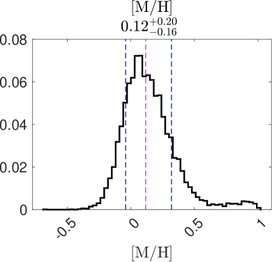
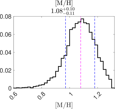
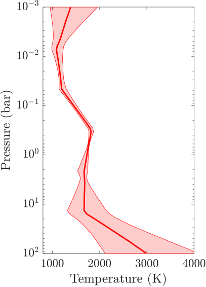
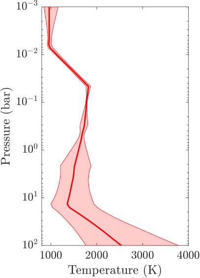
Figure 9: Left column - Posterior distributions for the secondary-eclipse retrieval of WASP-43b. The upper panel shows the posterior for the metallicity $[M/H]$, where the vertical, magenta line indicates the median of the distribution and the blue lines the corresponding 1-$\sigma$ intervals. The lower panel depicts the retrieved temperature-pressure profile. The thick, red line is the median temperature profile, while the shaded, red area is the 1-$\sigma$ interval of the temperature distribution. Right column - Same as in the left column for the high metallicity mode of the posterior distribution of [M/H].

The resulting temperature structure and the posterior distribution of metallicity [M/H] are shown in Fig. 9. The results suggest a metallicity of $0.1\pm 0.2$ that is consistent with slightly enhanced solar element abundances, in agreement with Stevenson et al. (2017) (0.3–1.7$\times$solar). This result is also consistent with the derived metallicity of the host star listed in Table 2. We note, however, that the data also supports a bimodal posterior distribution of the metallicity, with an additional higher-metallicity solution of [M/H]$\approx 1.08$ or roughly more than ten times solar metallicity. The corresponding posterior distributions are shown in the left column of Fig. 9. Since the host star is close to solar metallicity, we decided to isolate the low-metallicity peak from the posterior as our preferred solution by choosing an appropriate prior.

The temperature-pressure profile depicted in the lower panel of Fig. 9 is almost isothermal near pressures of 0.1 bar, without signs of a strong temperature inversion. This suggests that very strong shortwave absorbers like Fe, Fe+, or TiO are not a dominant opacity source in this atmosphere. The tightest constraints on the temperature profile are obtained for pressures between 1 bar and 0.1 bar. In the lower and upper atmosphere, on the other hand, the temperature-pressure profile is essentially prior-dominated.

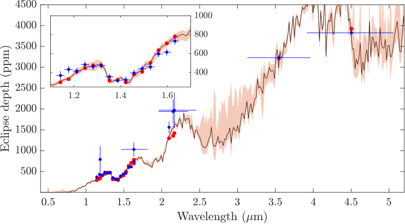
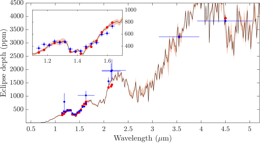
Figure 10: Top panel - Posterior distributions of the spectra and bandpass-integrated eclipse depths in units of ppm of the retrieval. The black line indicates the median spectrum, while the red, shaded area is the 1-$\sigma$ interval. Blue points denote the measured eclipse depths with their corresponding error bars while red points are the median, bandpass-integrated values from the posterior spectra. Their red error bars again indicate their corresponding 3-$\sigma$ intervals. The inset plot shows a magnification of the HST WFC3/G141 data. Bottom panel - Same as in the top panel for the high metallicity mode returned by our atmospheric retrieval.

Figure 10 shows the posterior eclipse depths for all bandpasses that have been included in the retrieval. The inset plot is a magnification of the HST WFC3/G141 data. Due to the lower error bars of the space-based data (HST WFC3/G141 and Spitzer), the retrieval is mostly driven by their reported eclipse depth. The ground-based data, on the other hand, seems to have a consistent shift towards higher eclipse depths compared to those obtained from the space telescopes. Due to their much larger errors, however, their impact on the resulting posteriors is only very minor.

In Fig. 10 we also plot, for comparison, the retrieved atmospheric model corresponding to the high metallicity mode in the $[M/H]$ posterior distribution. The two models, which are almost indistinguishable, fit all the data equally well, explaining the bimodality in the posterior distribution. At the current level of data precision we cannot a priori distinguish between the two solutions. We prefer the low metallicity mode based on the expectation that the metallicity of the planet should not significantly differ from that of its host star.

Table 7: Eclipse depth measurements of WASP-43b.

Passband or wavelength ($\mu$m)	Depth (ppm)	Ref.
UVIS/F350LP	¡140	this work
CHEOPS	80${}^{+60}_{-50}$	this work
TESS	70${}^{+50}_{-40}$	this work
1.186	790$\pm$320	Gillon et al. (2012)
2.095	1560$\pm$140	Gillon et al. (2012)
H	1030$\pm$170	Wang et al. (2013)
KS	1940$\pm$290	Wang et al. (2013)
GROND K	1970$\pm$420	Chen et al. (2014)
1.1425	367$\pm$45	Kreidberg et al. (2014); Stevenson et al. (2014, 2017)
1.1775	431$\pm$39	Kreidberg et al. (2014); Stevenson et al. (2014, 2017)
1.2125	414$\pm$38	Kreidberg et al. (2014); Stevenson et al. (2014, 2017)
1.2475	482$\pm$36	Kreidberg et al. (2014); Stevenson et al. (2014, 2017)
1.2825	460$\pm$37	Kreidberg et al. (2014); Stevenson et al. (2014, 2017)
1.3175	473$\pm$33	Kreidberg et al. (2014); Stevenson et al. (2014, 2017)
1.3525	353$\pm$34	Kreidberg et al. (2014); Stevenson et al. (2014, 2017)
1.3875	313$\pm$30	Kreidberg et al. (2014); Stevenson et al. (2014, 2017)
1.4225	320$\pm$36	Kreidberg et al. (2014); Stevenson et al. (2014, 2017)
1.4575	394$\pm$36	Kreidberg et al. (2014); Stevenson et al. (2014, 2017)
1.4925	439$\pm$33	Kreidberg et al. (2014); Stevenson et al. (2014, 2017)
1.5275	458$\pm$35	Kreidberg et al. (2014); Stevenson et al. (2014, 2017)
1.5625	595$\pm$36	Kreidberg et al. (2014); Stevenson et al. (2014, 2017)
1.5975	614$\pm$37	Kreidberg et al. (2014); Stevenson et al. (2014, 2017)
1.6325	732$\pm$42	Kreidberg et al. (2014); Stevenson et al. (2014, 2017)
Spitzer/IRAC3.6	3231$\pm$60	Stevenson et al. (2017)
Spitzer/IRAC4.5	3827$\pm$84	Stevenson et al. (2017)

In a post-process procedure of the retrieval, we estimated the predicted thermal emission in all short-wave bandpasses to decontaminate the measured eclipse depths. In particular, we computed the contribution to the eclipse depth in the HST WFC3/UVIS, CHEOPS and TESS LCs from the thermal emission by integrating the emission spectrum in the corresponding passbands. We did this computation for each step sampled by the retrieval analysis, thus obtaining for each instrument a population of contamination estimates that follows the posterior distribution of the expected thermal emission in the corresponding passband (Fig. 8). Afterwards, we randomly extracted an equally long subset of samples from the posterior distributions of the observed eclipse depth in the three passbands. Finally, for each instrument we decontaminated the observed eclipse depths by subtracting, sample by sample, the corresponding contamination from thermal emission. We thus obtained the reflection-only depths and the corresponding A_g by means of Eq. 9. The posterior distributions of the optical geometric albedos A_g in the three passbands are shown in Fig. 8: they are consistent among themselves and indicate that WASP-43b has a low geometric albedo. To get the most precise upper limit on A_g  we assumed no wavelength-dependence for A_g and multiply the three posterior distributions obtaining the combined posterior, shown in black in Fig. 8 after normalization. Following this last distribution function we can state that the albedo of the planet is lower than 0.087 at 99.9% confidence. This result is broadly consistent with the theoretical predictions of Sudarsky, Burrows, & Pinto (2000) and with ensembles of optical geometric albedos measured by Kepler (Heng & Demory 2013) and TESS (Wong et al. 2021).

6 Conclusions

In this work we provide a thorough analysis of the WASP-43 system. Using publicly available spectra we carried out a detailed spectroscopic characterization of the host star, confirming it as a late-K main sequence dwarf with solar metallicity and slow rotation, the latter supported also by spectroscopic and photometric activity indicators.

For a detailed characterization of the exoplanet, we analyzed the publicly available HST WFC3/UVIS and TESS photometry, together with dedicated CHEOPS observations of eleven individual occultations. We retrieved the transit, occultation and phase curve shapes while jointly modeling systematics (stellar and instrumental), ellipsoidal variations, gravity darkening and Doppler boosting.

We obtained a tentative detection of $A_{p}=100\pm 50$ ppm (Table 4) of the phase curve in the TESS data, and we found marginal evidence for a $\left(50^{+30}_{-20}\right)^{\circ}$ eastward phase offset (that is a peak before occultation). Previous infra-red observations also detected similar eastward peaks (Stevenson et al. 2014, 2017; Morello et al. 2019). The eastward offsets seen in the infra-red are in line with atmospheric circulation models of hot Jupiters that predict advection of hot material by means of equatorial jet streams (Showman & Guillot 2002). In this paradigm however, reflection-dominated phase curves are expected to peak after occultation, as reflective clouds are advected torwards the day side via the morning terminator (Esteves et al. 2015). WASP-43b however might deviate from this paradigm as the object is predicted to form clouds at all longitudes and at optical depths which cannot be probed by the data analyzed in this work (Helling et al. 2020; Venot et al. 2020). A local peak in reflectivity could be explained if local thermal and chemical conditions at the evening terminator are conducive to cloud condensation as well as cloud retention at observable altitudes.

Using all available eclipse depths in the infra-red, we perform a comprehensive modeling of the dayside atmosphere of WASP-43b. Our retrieval indicates that the metallicity of the atmosphere [M/H]=$0.1\pm$0.2 is consistent with the stellar counterpart, and compatible with previous estimates by Stevenson et al. (2017). The retrieval also suggests a non-inverted pressure-temperature profile at the sub-stellar point, which is common for mildly-irradiated hot Jupiters (e.g. Diamond-Lowe et al. 2014).

The model inferred from the infrared eclipses allowed us to extrapolate the thermal emission spectrum to optical wavelengths. We thus estimated the thermal emission contamination in the HST WFC3/UVIS, CHEOPS and TESS passbands and decontaminated the observed eclipse depths. This allowed us to put an upper limit to the geometric albedo A_g of the planet of 0.087 with a 99.9% confidence level, in agreement with Blažek et al. (2022). WASP-43b is thus quite similar in this regard to other “dark mirrors” such as, for example, TrES-2 b ($A_{\rm g}=0.0136^{+0.0022}_{-0.0033}$, Barclay et al. 2012), WASP-104 b ($A_{\rm g}<0.03$, Močnik, Hellier, & Southworth 2018) and 51 Peg b ($A_{\rm g}<0.20$, Scandariato et al. 2021; Spring et al. 2022). As discussed in, for example, Marley et al. (2013), the potential formation of high-temperature condensates for a solar-composition atmosphere starts around 2000 K, depending on pressure. Our inferred, high temperatures close to 2000 K at pressures between 1 bar and 0.1 bar on the dayside of WASP-43b, therefore, suggests that clouds are potentially either absent or form at pressures higher than those probed by our measurements. The low dayside albedos also indicate the absence of hazes that might form at higher altitudes.

7 Posterior distributions of the model parameters and best fit of TESS light curves

Figure 11: Corner plot of the MCMC chains of the jitter terms and normalization coefficients from the fit of the TESS LCs (see Sect. 4.1). The top right inset shows the corner plot for the GP parameters. In each plot, the solid blue lines mark the MAP values.

Figure 12: Corner plot of the MCMC chains of planetary parameters from the fit of the TESS LCs (see Sect. 4.1). The top right inset shows the corner plot for the phase curve amplitude and the phase offset. In each plot, the solid blue lines mark the MAP values.

8 Posterior distributions of the model parameters and best fit of CHEOPS light curves

9 Posterior distributions of the model parameters to fit HST WFC3/UVIS light curves