Rethink Decision Tree Traversal

Abstract

We will show how to implement binary decision tree traversal in the language of matrix computation. Our main contribution is to propose some equivalent algorithms of binary tree traversal based on novel matrix representation of the hierarchical structure of the decision tree. Our key idea is to travel the binary decision tree by maximum inner product search. We not only implement decision tree methods without the recursive traverse but also delve into the partitioning nature of tree-based methods.

1 Introduction

QuickScorer[12] and RapidScorer[21] are proposed based on bit-vectors of the false nodes in order to speed up the additive ensemble of regression trees in learning to rank. Inspired by [12], more works, such as [2; 11; 13; 15], focus on the application and acceleration of additive tree models while we will pay attention to the theory of algorithms specially the representation of binary decision tree in the language of matrix computation.

Based on so-called Tree Supervision Loss, a hierarchical classifier is built from the weights of the softmax layer in convolutional neural networks in [18]. In [20; 19], tree regularization is used to enhance the interpretability of deep neural networks. A generalized tree representation termed TART is based on transition matrix shown in [22]. We introduce some matrix to represent the structure of binary decision tree, which means that matrix can imply hierarchy. And we will show how to generate equivalent algorithms of binary tree traversal, which is to translate the binary decision tree to matrix computation.

We begin with the algorithm 1 and provide some illustration. Then we modify 1 to matrix computation, where we introduce bit-matrix and sign-matrix to represent the decision tree structure. And we consider binary decision tree evaluation as error-correcting output codes. Later we discuss the interpretable representation. Finally we give a summary.

2 QuickScorer

The QuickScorer is a tree-based rank model, which has reduced control hazard, smaller branch mis-prediction rate and better memory access patterns in experiment [12]. The core of QuickScorer is to represent the candidate exit leaves with a bitvetor [12] as shown in algorithm (1). Based on the bit-vectors of false nodes, tree traversal is via the bitwise logical $\mathit{AND}$ operations when all the results of associated test evaluation are known as shown in algorithm (1). Its correctness is originally proved in [12]. More implementation or extension of QuickScorer can be found in [2; 11; 13; 21; 15].

Given a tree $T(N,L)$, the traversal of the input $\mathbf{x}$ is described in algorithm 1 and its correctness is proved in [12]. Here we follow the description of tree model in [12].

A decision tree $T(N,L)$ is composed of a set of internal nodes $N=\{n_{0},n_{1},\cdots,n_{t}\}$ and and a set of leaves $L=\{l_{0},l_{1},\cdots,l_{t+1}\}$ where each $n\in N$ is associated with a Boolean test and each leaf $l\in L$ stores the prediction $l.val\in\mathbb{R}$. All the nodes whose Boolean conditions evaluate to $False$ are called false nodes, and true nodes otherwise. If a visited node in $N$ is a false one, then the right branch is taken, and the left branch otherwise.

Hereinafter, we assume that nodes of $T$ are numbered in breadth-first order and leaves from left to right.

Algorithm 1 Scorer of QuickScorer

1:Input:

• input feature vector $\mathbf{x}$

• a binary decision tree $T(N,L)$ with

  • internal nodes $N$: $\{n_{0},\cdots,n_{t-1}\},1\leq t<\infty$

  • a set of leaves $L$: $\{l_{0},\cdots,l_{t}\},1\leq t<\infty$

  • the prediction of leaf $l\in L$ :$l.val\in\mathbb{R}$

  • node bitvector associated with $n\in N$: $n.bitvector$

2:Output: tree traversal output value

3:procedure Score($\mathbf{x},T$)

4:     Initialize the result bitvector $\mathbf{v}\leftarrow 1,1,\cdots,1$

5:     Find the $Fasle$ nodes $U(\mathbf{x},T)$ given $\mathbf{x},T$

6:     for  node $u\in U$ do $\triangleright$ iterate over the false nodes

7:         $\vec{v}\leftarrow\vec{v}\wedge u.bitvector$ $\triangleright$ update by logical $\mathit{AND}$      

8:     $j\leftarrow$ index of the leftmost bit set to 1 of $\vec{v}$

9:     return $l_{j}.val$

It is best to read [12] for more details on how to evaluate a single binary decision tree stored as a set of precomputed bitvectors. Here we adopt the illustration from [16] in figure (1) and (2).

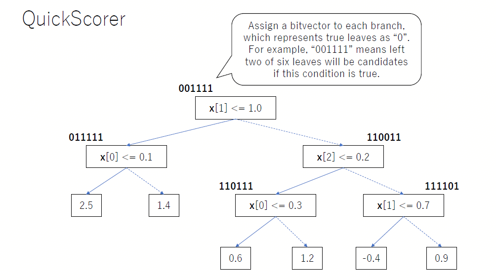
Figure 1: The bitvector in QuickScorer

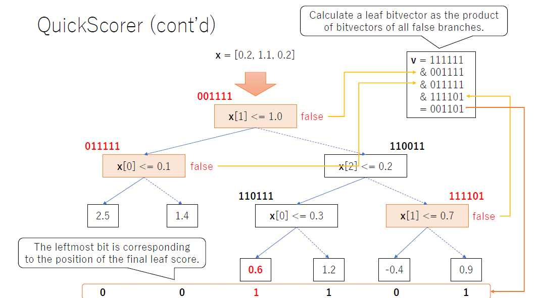
Figure 2: The scorer in QuickScorer

2.1 Construction of Bit-vectors and Bit-matrix

In this section, we will introduce the construction of the bit-matrix based on (1).

In [12], the idea of tree traversal using bitvectors is based on the node bitvector as below:

Every internal node $n$ is associated with a node bitvector $n.bitvector$ (of the same length), acting as a bitmask that encodes (with 0’s) the set of leaves to be removed from $L$ whenever $n$ is a false node.

In [21], QuickScorer is described as below

QuickScorer maintains a bitvector, composed of $\wedge$ bits, one per leaf, to indicate the possible exit leaf candidates with corresponding bits equal to 1.

We call the bit-vector in QuickScorer as bit-vector for false node defined in (1).

Definition 1

The bit-vector for a false node is defined as a binary vector in $\{0,1\}^{n}$ if the decision tree has $n$ internal nodes, where the digit 1 corresponds to the possible exit leaf candidates and the digit 0 corresponds to the impossible exit leaf when the associated Boolean test is false.

The last bit is always equal to 1 in each bitvector by definition.

Now we consider the simplest case : (1) all internal nodes are true; (2) all internal nodes are false. In the first case, there is no false nodes and the result bitvector $v$ is only initialized in algorithm 1. Thus, the first bit must correspond to the leftmost leaf. In the second case, there is no true nodes and the result bitvector $v$ is bit-wise logical $\mathit{AND}$ of all bitvectors in the tree, where the rightmost leaf must be indicated by 1.

Definition 2

The bit-matrix $\mathrm{B}$ of a decision tree is a binary matrix where each column is the bitvector of the tree.

The simplest bit-matrix is $\begin{pmatrix}0\quad 1\\ \end{pmatrix}^{T}$. The bit-matrix of the decision tree in figure (1) is given as follows.

$$B=\begin{pmatrix}0&0&1&1&1\\ 0&1&1&1&1\\ 1&1&0&0&1\\ 1&1&0&1&1\\ 1&1&1&1&0\\ 1&1&1&1&1\\ \end{pmatrix}.$$

The next is to show the relation between the structure of decision tree and its bit-matrix.

2.2 Some Properties of Bit-matrice

By the definition 2, the bit-matrix is binary matrix. Here we want to search some properties of the bit-matrix of a binary decision tree specially its rank.

Definition 3

The complement of the bitvector $b$ denoted by $c$ is defined by

$$b+c=\vec{1}.$$

For example, the complement of $\begin{pmatrix}0\quad 1\\ \end{pmatrix}^{T}$ is $\begin{pmatrix}1\quad 0\\ \end{pmatrix}^{T}$.

The complement bit-vectors of a node is a binary vector where the digit 1 corresponds to the possible exit leaf candidates over its subtree when it is a true node. The bitvector $b$ and its complement bitvector $\vec{1}-b$ cannot exist in the same bit-matrix of a decision tree.

We can calculate a leaf bitvector as the product of bit-vectors of false nodes and complement bit-vectors of true nodes. For example, the bitvectors of the false nodes are $111111$, $001111$, $011111$, $111101$, $001101$ and complement bit-vectors of true nodes are $001100$ and $001000$. And their product is $001000$ which indicates the exit leaf directly

Lemma 1

The bitvector $b$ is linearly independent of its complement bitvector $\vec{1}-b$.

Lemma 2

The bitvectors of the right subtree are linearly independent of the bitvectors of the left subtree.

Proof 2.1

By the definition, the bits corresponding to the exit leaf candidates of the left subtree are always set to 1 in the bitvectors of the right subtree while there is at least one $0$-bit corresponding to the exit leaf candidates of the left subtree in the bitvectors of the left subtree. Thus this lemma is completed.

Based on the above lemma, we can obtain the following theorem 1.

Theorem 1

The bit-matrix $B$ is invertible for any decision tree.

Proof 2.2

We use induction. The induction hypothesis is that $(B_{n\times(n-1)})$ is invertible for all integer $n\geq 2$.

When $n=2$, we have $B=\begin{pmatrix}0\quad 1\\ \end{pmatrix}^{T}$ so it holds.

Assume that $(B_{n\times(n-1)})$ is invertible if $t\leq N$, we will prove that $(B_{(N+1)\times N})$ is invertible. By the assumption, it holds for the right subtree and left subtree. By the above lemma, it holds for the whole tree.

As above, it holds for all integer $n\geq 2$ by induction.

From 1 we can find that the augmented matrix $(B_{n\times(n-1)}\,\,\vec{1}_{n})$ invertible. The rank is an invariant of bit-matrices if their size is determined. The column is unique and distinct in the matrix $B$, where the digit 1/0 corresponds to the possible/impossible exit leaf when the associated Boolean test is false.

The augmented matrix $(B\,\,\vec{1})$ of the tree in 1 is symmetric but the coding scheme of bitvectors is based on the false nodes. This symmetry is emergent.

The structure of a decision tree is determined by its bit-matrix and the structure of the subtree is determined by a submatrix of the bit-matrix. And we can observe that recursive patterns emerge in the bit-matrix as below.

$$\left[\begin{array}[]{c|c|cccc}0&0&1&1&1\\ 0&1&1&1&1\\ 1&1&0&0&1\\ 1&1&0&1&1\\ 1&1&1&1&0\\ 1&1&1&1&1\end{array}\right],\left[\begin{array}[]{ccc}0&0&1\\ 0&1&1\\ 1&1&0\\ 1&1&1\end{array}\right].$$

The hierarchy of the tree is encoded in the position order of bitvectors.

3 Beyond Bitvector: Diverse Tree Evaluation

We will convert the bitwise logical $\mathit{AND}$ operation to multiplication of binary matrix and vector. Specially, we focus on how to implement binary decision tree in the language of matrix computation.

3.1 The Computational Perspective

There are two key steps of QuickScorer:(1) the first is to find the false nodes given the input and tree; (2) the second is to find the terminal node based on the bitvectors of false nodes. Here, we will implement these steps in the language of matrix computation.

From the computational perspective, the of logical $\mathit{AND}$ of bitvectors is equivalent to their element-wise multiplication n algorithm (1)

$$S_{F}=\arg\max(\underset{u\in U}{\wedge}u.bitvector)=\arg\max(\underset{u\in U}{\prod}u.bitvector).$$ (1)

So the index of the bit set to 1 of logical $\mathit{AND}$ in algorithm (1) requires that all operand must be 1 in the index corresponding to the bit set to 1 of $\vec{v}$. And it is equivalent to the intersection $\cap_{u\in U}\arg\max(u.bitvector)$ by combining the fact that 1 is the maximum of the bitvector in algorithm (1). Then we can replace the logical $\mathit{AND}$ operation in the algorithm (1) with the matrix computation operation based on the following relation

$$S_{F}=\underset{u\in U}{\cap}\arg\max(u.bitvector)=\arg\max(\sum_{u\in U}u.bitvector).$$ (2)

The step to find the false nodes in (1) is to evaluate all the Boolean tests of internal nodes and we use a binary vector to represent such procedure as defined in (4).

Definition 4

The test vector $\vec{t}$ of the input $\mathbf{x}$ is a binary column vector where the digit 1 corresponds to the false node and the digit 0 corresponds to the true node for a given tree $T(N,L)$.

Based on the test vector $\vec{t}$ and bit-matrix $B$, we replace the logical $\mathit{AND}$ over the bitvectors of false nodes by the matrix computation as below:

$$\vec{v}=B\vec{t}+\vec{1}$$ (3)

where $\vec{1}$ is a bitvector with all bits set to 1.

The matrix-vector multiplication $B\vec{t}$ is the sum of bitvectors of all false nodes. The key observation is that the maximum of formula (3) corresponds to bit set to 1 of the result bitvector in algorithm (1). In another word, $\arg\max$ of formula (3) is equal to $\arg\max$ of the result vector in algorithm (1), where the operator $\arg\max$ returns all the index of maximum in the vector. Additionally, finding the index of leftmost maximum of formula (3) is to find the minimum index in $\arg\max$ of formula (3).

And we can obtain the theorem (2).

Theorem 2

The algorithm (1) is equivalent to the algorithm (2).

Algorithm 2 Scorer of QuickScorer in language of matrix computation

1:Input:

• a feature vector $\mathbf{x}$

• a binary decision tree $T(N,L)$ with

  • internal nodes $N$: $\{n_{0},\cdots,n_{t-1}\},1\leq t<\infty$

  • a set of leaves $L$: $\{l_{0},\cdots,l_{t}\},1\leq t<\infty$

  • the prediction of leaf $l\in L$ :$l.val\in\mathbb{R}$

  • the bit-matrix of $T(N,L)$: $B$

2:Output: tree traversal output value

3:procedure Scorer($\mathbf{x},T$)

4:     Find the test vector $\vec{t}$ given $\mathbf{x},T$ $\triangleright$ as defined in 4

5:     Compute the result vector: $\vec{v}\leftarrow B\vec{t}+\vec{1}$ $\triangleright$ tree traversal via matrix operation

6:     $j\leftarrow\min\arg\max{\vec{v}}$ $\triangleright$ index of the leftmost maximum of $\mathbf{v}$

7:     return $l_{j}.val$

The matrix-vector multiplication is the linear combination of column vector, so

$$B\vec{t}=\sum_{i}t_{i}B_{i},$$

where $B_{i}$ is the $i$-th bitvector. And we can obtain the following relation:

$$S_{F}=\arg\max(B\vec{t}+\vec{1})=\arg\max(\sum_{i}t_{i}B_{i})=\arg\max(\sum_{i}p_{i}t_{i}B_{i})$$

if each $p_{i}$ is positive. Thus, the non-negative number is sufficient for the test vector $\vec{t}$ and bitmatrix $B$. In another word, we extend the algorithm 1 from binary value to non-negative value.

Another observation of $B\vec{t}$ is that $\arg\max B\vec{t}=\cap_{i}\arg\max(t_{i}B_{i})$. Let $\tilde{B}_{i}$ replace the 0 in $B_{i}$ by $-1$, then we can find the following equation

$$\arg\max B\vec{t}=\cap_{i}\arg\max(t_{i}B_{i})=\cap_{i}\arg\max(t_{i}\tilde{B}_{i})=\arg\max(\sum_{i}t_{i}\tilde{B}_{i}),$$ (4)

so bit-matrix is not necessary for the algorithm (1).

In contrast to [12], we can define the bitvector for the true node acting as a bitmask that encodes (with 0’s) the set of leaves to be removed whenever the internal node is a true node. The bitwise logical $\mathit{AND}$ between $\vec{1}$ and the node bitvector of a true node $n$ corresponds to the removal of the leaves in the right subtree of $n$ from the candidate exit leaves. And we can obtain the following equation

$$S_{T}=\arg\max(\underset{t\in T}{\prod}t.bitvector)=\underset{t\in T}{\cap}\arg\max(t.bitvector)$$

where $T$ is the true node of a decision tree and $t.bitvector$ is the bitvector for the internal node $t$. The exit leaf cannot removed by the logical $\mathit{AND}$ of these bitvectors but leftmost bit set to 1 does not correspond to the exit leaf. In another word, we have the following relation $S_{T}\setminus S_{F}\not=\emptyset$ and $\min(S_{T}\cap S_{F})=\min S_{F}$ where $S_{F}$ is defined in 2.

The inner product between the $i$-th column of the $B$ and the test vector $\vec{t}$ is the $i$-th value of $B\vec{t}$, which is the number of false nodes that select the $i$-th candidate leaf. And the maximum of $B\vec{t}$ is the number of all false nodes, which is equal to $\left<\vec{t},\vec{t}\right>$ or the $\ell_{1}$ norm of $\vec{t}$ and independent of the norm of column vectors of $B$.

However, computation procedures can be equivalent in form but different in efficiency. The $\arg\max$ and intersection operation may take more time to execute. And these diverse equivalent form will help us understand the algorithm further. In algorithm 2, we replace the procedure to find the false nodes and the iteration over the false nodes in algorithm 1 with the test vector and matrix-vector multiplication.

These observation and facts imply the possibility to design more efficient algorithms equivalent to the algorithm (1). We can find more substitute for the bit-matrix encoding schemes. In contrast to [18], we find that the hierarchy of each node is embedding in the column vectors of the bit-matrix. In algorithm (1), it is the index of leftmost bit set to 1 in the result vector that we only require, which is the index of the exit leaf that we really need during tree traversal when the input $\mathbf{x}$ and the decision tree $T$ are given. Next we will introduce how to construct an algorithm based on the unique and constant maximum to traversal the binary tree.

3.2 The Algorithmic Perspective

The algorithm QuickScorer in [12] looks like magicians’ trick and its lack of intuitions makes it difficult to understand the deeper insight behind it. The bitvector is position-sensitive in algorithm 1, where the nodes of are required to be numbered in breadth-first order and leaves from left to right.

Since the reachability of a leaf node is only determined by the internal nodes over the path from its root to itself, it is these bitvectors in algorithm (1) that play the lead role during traversal rather than the bitvectors of other false nodes. Thus we should take it into consideration when designing new test vector $\vec{s}$.

Definition 5

The signed test vector $\vec{s}$ of the input $\mathbf{x}$ is a binary vector where the digit $1$ corresponds to the false node and the digit $-1$ corresponds to the true node for a given decision tree.

By comparing definition 1 and 5, we can find the equation $\vec{s}=2\vec{t}-\vec{1}$.

We only consider the matrix-vector $B\vec{t}$ in 3 as the linear combination of bitvectors while it is the inner products of the column vectors of $B$ and test vector $\vec{t}$ that determine the maximum of $B\vec{t}$. The bitvectors as rows in matrix $B$ is designed for the internal nodes rather than the leaf nodes.

We need to design vectors to represent the leaf node as the column vector and ensure that the inner product of the leaf vector and the test vector is equal to the number of the internal nodes over the path from the root node to itself if the input reaches this leaf node.

Definition 6

The representation vector of a leaf node is a ternary vector determined by the following rules:

• the digit $+1$ corresponds to the true nodes over its path from the root node;

• the digit $-1$ corresponds to the false nodes over its path from the root node;

• and digit $0$ corresponds to the rest of internal nodes.

The representation vector of a leaf node actually describes the path from the root to this leaf node, which contains the encoding character: $-1$ represents an edge to a left child, and $+1$ represents an edge to a right child. And we defined the signed matrix to describe the stricture of the binary decision tree as 7.

Definition 7

The signed matrix $S$ of a decision tree consists of its leaf representation vectors as its row vector.

It is easy to find the upper bound of the inner product of a leaf vector $\vec{p}=(p_{1},\cdots,p_{d})^{T}\in\{+1,0,-1\}^{d}$ and the signed test vector $\vec{s}=(s_{1},\cdots,s_{d})^{T}\in\{1,-1\}^{d}$ as shown below

$$\left<\vec{p},\vec{s}\right>=\sum_{i=1}^{d}p_{i}s_{i}\leq\sum_{i=1}^{d}|p_{i}|=\|\vec{p}\|_{1}.$$ (5)

If $p_{i}s_{i}>0$, we say that the leaf node and the input reach a consensus on the $i$-th test.

Definition 8

The depth of a leaf node is the path length measured as the number of non-terminal nodes between the root node and itself. The depth vector $\vec{d}$ of a decision tree consists of all leaf nodes depth and depth matrix $D$ is defined as $\operatorname{diag}(\vec{d})$.

If the number of consensuses reached between the input and the leaf node is equal to the depth of the leaf node, then the leaf is the destination of the input in the decision tree.

We propose the algorithm termed SignQuickScorer as (3).

Algorithm 3 SignQuickScorer

1:Input:

• a feature vector $\mathbf{x}$

• a binary decision tree $T$

2:Output: tree traversal output value

3:procedure SignQuickScorer($\mathbf{x},T$)

4:     Find the signed test vector $\vec{s}$ given $\mathbf{x},T$ $\triangleright$ as defined in 5

5:     Compute the result vector: $\vec{v}\leftarrow D^{-1}S\vec{s}$ $\triangleright$ $D^{-1}$ and $S$ are precomputed in 7 8.

6:     $j\leftarrow\arg\max\vec{v}$ $\triangleright$ index of the maximum of $\mathbf{v}$

7:     return $l_{j}.val$

Theorem 3

The algorithm SignQuickScorer(3) is correct.

Proof 3.1

We only need to prove the inner product of the normalized exit leaf vector $\frac{s^{\ast}}{\left<s^{\ast},s^{\ast}\right>}$ and the test vector $\vec{t}$ is the unique maximum of $D^{-1}S\vec{t}$.

First, we prove that $\frac{\left<s^{\ast},\vec{t}\right>}{\left<s^{\ast},s^{\ast}\right>}=\max\{D^{-1}S\vec{t}\}$. And $\max_{b\in\mathbb{B}}\left<t,b\right>=\left<t,b^{\ast}\right>=\left<t,t\right>$ if and only if $\left<t-b^{\ast},t\right>=0$ by the inequality 5. Thus $\frac{\left<s^{\ast},\vec{t}\right>}{\left<s^{\ast},s^{\ast}\right>}\leq 1$. And according to the definition 5 and 6, we have $\left<s^{\ast},\vec{t}-s^{\ast}\right>=0$ and imply that $\left<s^{\ast},\vec{t}\right>=\left<s^{\ast},s^{\ast}\right>$ so $\max\{D^{-1}S\vec{t}\}=1$.

For the rest of leaf vectors $s\in T$ and the test vector $\vec{t}$ we have the equation: $\left<s,\vec{t}\right><\left<s,s\right>$because there is at least one test which the input does not match over the path from the root node to this leaf node. So that $\left<s,\vec{t}-s\right>\not=0$. And we complete this proof.

And the result vector can be divided element-wisely by the number of the internal nodes over the path, then we can obtain the unique maximum as the indicator of the exit leaf.

We can take the example in figure 2 as follows

$$\vec{s}=\begin{pmatrix}1\\ 1\\ -1\\ -1\\ +1\\ \end{pmatrix},S=\begin{pmatrix}-1&-1&0&0&0\\ -1&+1&0&0&0\\ +1&0&-1&-1&0\\ +1&0&-1&+1&0\\ +1&0&+1&0&-1\\ +1&0&+1&0&+1\\ \end{pmatrix},D=\begin{pmatrix}2&0&0&0&0&0\\ 0&2&0&0&0&0\\ 0&0&3&0&0&0\\ 0&0&0&3&0&0\\ 0&0&0&0&3&0\\ 0&0&0&0&0&3\\ \end{pmatrix},D^{-1}S\vec{s}=\begin{pmatrix}-1\\ 0\\ 1\\ \frac{1}{3}\\ -\frac{1}{3}\\ \frac{1}{3}\end{pmatrix}.$$

And we can regard the algorithm (3) as the decoding of error-correcting output coding [4; 5] shown in (4), which is deigned for multi-classification by combining binary classifiers. Both methods believe on the cluster assumption, which is based on the similarity in essence.

Algorithm 4 SignQuickScorer as template matching

1:Input:

• a feature vector $\mathbf{x}$

• a binary decision tree $T$

2:Output: tree traversal output value

3:procedure SignQuickScorer($\mathbf{x},T$)

4:     Find the test vector $\vec{t}$ given $\mathbf{x},T$ $\triangleright$ as defined in 5

5:     Find the most likely template: $j\leftarrow\arg_{i}\max\frac{\left<S_{i},\vec{t}\right>}{\vec{d}_{i}}$ $\triangleright$ $S_{i}$ is the $i$-thh column of $S$

6:     return $l_{j}.val$.

Each class is attached to an unique code in error-correcting output coding(ECOC) [3; 10; 1] while a leaf vector only indicates a specific region of the feature space and each class may be attached to more than one leaves in (3). And the key step in (4) is find the maximum similarity, while key step in (3) is to find the maximum scaled inner product. The value attached to the leaf node is voted by majority or averaging which is different from other mixed regression method[6].

Next we will show how to take advantage of the unique maximizer of $D^{-1}S\vec{s}$.

3.3 The Representation Perspective

We define the $\delta$ function to replace the $\max$ operator in (3) as following:

$$\delta(x)=\begin{cases}0&x\not=0\\ 1&x=0\end{cases}\quad\forall x\in\mathbb{R}.$$

According to the proof of 3, we can find the index of the leftmost maximum of $\vec{v}$ by the following equation

$$j=\sum_{i}\delta(\vec{v}_{i}-1)i$$

because that $\max\vec{v}=1$ and $\arg\max\vec{v}$ is unique, where $\mathbf{v}=D^{-1}S\vec{t}$.

And we find a succinct expression of 3 as shown in algorithm 5.

Algorithm 5 SignQuickScorer as Attention

1:Input:

• a feature vector $\mathbf{x}$

• a binary decision tree $T$

2:Output: tree traversal output value

3:procedure SignQuickScorer($\mathbf{x},T$)

4:     Find the test vector $\vec{t}$ given $\mathbf{x},T$ $\triangleright$ as defined in 5.

5:     Compute the result vector: $\vec{v}\leftarrow D^{-1}S\vec{t}$ $\triangleright$ as computed in 3.

6:     return $\sum_{i}\delta(\vec{v}_{i}-1)l_{i}.val$

We can explain this $\delta$ function as selector in order to find the most likely prediction value.

Note that $\vec{v}_{i}-1\iff\frac{\left<S_{i},\vec{t}\right>}{\vec{d}_{i}}=1\iff\left<S_{i},\vec{t}\right>=\vec{d}_{i}$ so we can obtain a variant of the algorithm (3) as shown in (6).

Algorithm 6 SignQuickScorer

1:Input:

• a feature vector $\mathbf{x}$

• a binary decision tree $T$

2:Output: tree traversal output value

3:procedure SignQuickScorer($\mathbf{x},T$)

4:     Find the test vector $\vec{t}$ given $\mathbf{x},T$ $\triangleright$ $\vec{t}$ defined in 5.

5:     Compute the result vector: $\vec{v}\leftarrow S\vec{t}-\vec{d}.$ $\triangleright$ $S,\vec{d}$ defined in (7), (8), respectively.

6:     return $\sum_{i}\delta(\vec{v}_{i})l_{i}.val$

In terms of attention mechanism [17; 14; 9], the decision tree is in the following form:

$$T(\mathbf{x})=\sum_{i}\delta({(D^{-1}S\vec{t})}_{i}-1)l_{i}.val=\operatorname{Attention}(\vec{t},S,l)$$ (6)

where the weight assigned to each value is computed by the following function

$$w_{i}=\delta({(D^{-1}S\vec{t})}_{i}-1)=\begin{cases}0&{(D^{-1}S\vec{t})}_{i}\not=1\\ 1&otherwise\end{cases}.$$

In fact, it is the hard attention. And we can output a soft attention distribution by applying the scaled dot-product scoring function instead of the $\delta$ function as below

$$w_{i}=\frac{\exp({(D^{-1}S\vec{t})}_{i})}{\sum_{i}\exp({(D^{-1}S\vec{t})}_{i})}.$$

Similarly, we can discover that the soft decision tree is the soft attention.

The Boolean expression may occur in different path so that we can rewrite the signed test vector $\vec{s}$ as a selection of the raw Boolean expression $\vec{s}=M\vec{e}$, where the matrix $M$ describe the contribution of each Boolean expression and the importance of each attribute.

It is a general consensus that decision trees are of interpretability. Interpretablity is partially dependent on the model complexity. For some model sparsity is a proxy for interpretability. However, interpretability is independent of the model complexity for decision trees because of their explicit decision boundaries. Thus, the algorithm 5 provides an interpretable explanation of hard attention.

In [24; 23], we restricted the input vector in numerical data. The difficulty is to handle the hybrid data. The method 5 is a general scheme on how to convert the rule-based methods to the attention mechanism. And test vector $\vec{t}$ is the feature vector in $\{+1,-1\}^{d}$ extracted from the raw feature space and we only need $d+1$ patterns determined by the leaf vector in $\{+1,0,-1\}^{d}$, where different patterns may share the same value.

Each path in decision trees consists of Boolean interactions of features [bin_yu]. The lack of feature transformation in (3), (4), (5) may restrict their predictability and stability. We can discover that the most expensive computation of (3), (4), (5) and (6) is maximum inner product search, which belong to the nearest neighbor search problem.

The binary decision tree traversal is a router/gate based on Boolean tests, which select a destination leaf node. For example, the centroid of the $i$-th leaf node is to minimize

$$\sum_{\mathbf{x}\in\mathcal{X}}\delta(\vec{v}_{i}-1)d(\mathbf{x},c_{i})$$

and the value of the $i$-th leaf node is to minimize

$$\sum_{(\mathbf{x},y)\in\mathcal{X}\times\mathcal{Y}}\delta(\vec{v}_{i}-1)d(y,l_{i}.val)$$

where $v_{i}$ is dependent of $\mathbf{x}$ as computed in algorithm (5); $d(\cdot,\cdot)$ is the quasi-distance function. Ensemble and mixture essence occurs in the decision tree. We would like find the prototype sample of each leaf node and convert the decision problem into nearest neighbor search directly while it is beyond our scope here.

4 Discussion

We clarify some properties of the bit-matrix of decision tree in QuickScorer. And we introduce the emergent recursive patterns in the bit-matrix and some equivalent algorithms of QuickScorer, which is to evaluate the binary decision tree in the language of matrix computation. Our main contribution is to propose some novel methods to perform decision tree traversal from different perspectives.

References

- [1] Erin L Allwein, Robert E Schapire, and Yoram Singer. Reducing multiclass to binary: a unifying approach for margin classifiers. Journal of Machine Learning Research, 1(2):113–141, 2001.
- [2] Domenico Dato, Claudio Lucchese, Franco Maria Nardini, Salvatore Orlando, Raffaele Perego, Nicola Tonellotto, and Rossano Venturini. Fast ranking with additive ensembles of oblivious and non-oblivious regression trees. ACM Transactions on Information Systems (TOIS), 35(2):1–31, 2016.
- [3] Thomas G Dietterich and Ghulum Bakiri. Solving multiclass learning problems via error-correcting output codes. Journal of Artificial Intelligence Research, 2(1):263–286, 1994.
- [4] Sergio Escalera, Oriol Pujol, and Petia Radeva. Decoding of ternary error correcting output codes. pages 753–763, 2006.
- [5] Escalerasergio, Pujoloriol, and Radevapetia. On the decoding process in ternary error-correcting output codes. IEEE Transactions on Pattern Analysis and Machine Intelligence, 2010.
- [6] Kun Gai, Xiaoqiang Zhu, Han Li, Kai Liu, and Zhe Wang. Learning piece-wise linear models from large scale data for ad click prediction. arXiv: Machine Learning, 2017.
- [7] Jiun Tian Hoe, Kam Woh Ng, Tianyu Zhang, Chee Seng Chan, Yi-Zhe Song, and Tao Xiang. One loss for all: Deep hashing with a single cosine similarity based learning objective. In M. Ranzato, A. Beygelzimer, Y. Dauphin, P.S. Liang, and J. Wortman Vaughan, editors, Advances in Neural Information Processing Systems, volume 34, pages 24286–24298. Curran Associates, Inc., 2021.
- [8] Rong Kang, Yue Cao, Mingsheng Long, Jianmin Wang, and Philip S. Yu. Maximum-margin hamming hashing. 2019 IEEE/CVF International Conference on Computer Vision (ICCV), pages 8251–8260, 2019.
- [9] A. Katharopoulos, A. Vyas, N. Pappas, and F. Fleuret. Transformers are RNNs: Fast autoregressive transformers with linear attention. In Proceedings of the International Conference on Machine Learning (ICML), 2020.
- [10] Eun Bae Kong and Thomas G. Dietterich. Error-correcting output coding corrects bias and variance. In In Proceedings of the Twelfth International Conference on Machine Learning, pages 313–321. Morgan Kaufmann, 1995.
- [11] Francesco Lettich, Claudio Lucchese, Franco Nardini, Salvatore Orlando, Raffaele Perego, Nicola Tonellotto, and Rossano Venturini. GPU-based parallelization of QuickScorer to speed-up document ranking with tree ensembles. In 7th Italian Information Retrieval Workshop, IIR 2016, volume 1653. CEUR-WS, 2016.
- [12] Claudio Lucchese, Franco Maria Nardini, Salvatore Orlando, Raffaele Perego, Nicola Tonellotto, and Rossano Venturini. QuickScorer: A fast algorithm to rank documents with additive ensembles of regression trees. In Proceedings of the 38th International ACM SIGIR Conference on Research and Development in Information Retrieval, pages 73–82, 2015.
- [13] Claudio Lucchese, Franco Maria Nardini, Salvatore Orlando, Raffaele Perego, Nicola Tonellotto, and Rossano Venturini. QuickScorer: Efficient traversal of large ensembles of decision trees. In Joint European Conference on Machine Learning and Knowledge Discovery in Databases, pages 383–387. Springer, 2017.
- [14] Hideya Mino, Masao Utiyama, Eiichiro Sumita, and Takenobu Tokunaga. Key-value attention mechanism for neural machine translation. In Proceedings of the Eighth International Joint Conference on Natural Language Processing (Volume 2: Short Papers), pages 290–295, Taipei, Taiwan, November 2017. Asian Federation of Natural Language Processing.
- [15] Romina Molina, Fernando Loor, Veronica Gil-Costa, Franco Maria Nardini, Raffaele Perego, and Salvatore Trani. Efficient traversal of decision tree ensembles with FPGAs. Journal of Parallel and Distributed Computing, 155:38–49, 2021.
- [16] Shitoumu. On quick scorer predication of the additive ensembles of regression trees model. Website. Accessed March 22, 2022.
- [17] Ashish Vaswani, Noam Shazeer, Niki Parmar, Jakob Uszkoreit, Llion Jones, Aidan N Gomez, Ł ukasz Kaiser, and Illia Polosukhin. Attention is all you need. In I. Guyon, U. V. Luxburg, S. Bengio, H. Wallach, R. Fergus, S. Vishwanathan, and R. Garnett, editors, Advances in Neural Information Processing Systems 30, pages 5998–6008. Curran Associates, Inc., 2017.
- [18] Alvin Wan, Lisa Dunlap, Daniel Ho, Jihan Yin, Scott Lee, Henry Jin, Suzanne Petryk, Sarah Adel Bargal, and Joseph E. Gonzalez. NBDT: Neural-backed decision trees, 2020.
- [19] Mike Wu, Michael C. Hughes, Sonali Parbhoo, Maurizio Zazzi, Volker Roth, and Finale Doshi-Velez. Beyond sparsity: Tree regularization of deep models for interpretability. In Proceedings of the Thirty-Second AAAI Conference on Artificial Intelligence and Thirtieth Innovative Applications of Artificial Intelligence Conference and Eighth AAAI Symposium on Educational Advances in Artificial Intelligence, AAAI’18/IAAI’18/EAAI’18. AAAI Press, 2018.
- [20] Mike Wu, Sonali Parbhoo, Michael C. Hughes, Volker Roth, and Finale Doshi-Velez. Optimizing for interpretability in deep neural networks with tree regularization. J. Artif. Int. Res., 72:1–37, jan 2022.
- [21] Ting Ye, Hucheng Zhou, Will Y Zou, Bin Gao, and Ruofei Zhang. RapidScorer: fast tree ensemble evaluation by maximizing compactness in data level parallelization. In Proceedings of the 24th ACM SIGKDD International Conference on Knowledge Discovery & Data Mining, pages 941–950, 2018.
- [22] Jaemin Yoo and Lee Sael. Transition matrix representation of trees with transposed convolutions. In Proceedings of the 2022 SIAM International Conference on Data Mining (SDM). SIAM, 2022.
- [23] Jinxiong Zhang. Decision machines: Interpreting decision tree as a model combination method. ArXiv, abs/2101.11347, 2021.
- [24] Jinxiong Zhang. Yet another representation of binary decision trees: A mathematical demonstration. ArXiv, abs/2101.07077, 2021.