The enhanced soliton propagation and energy transfer in the coupled drift wave and energetic-particle-induced geodesic acoustic mode system

Abstract

The evolution of the coupled drift wave (DW) and energetic-particle-induced geodesic acoustic mode (EGAM) nonlinear system is investigated using the fully nonlinear coupled DW-EGAM two-field equations, with emphasis on the turbulence spreading in the form of soliton and the nonlinear energy transfer between DW and EGAM. Four scenarios with different combinations of EGAM initial amplitudes and linear EGAM growth rates are designed to delineate the effects of linear EGAM drive and finite EGAM amplitude on DW nonlinear dynamic evolution. In presence of the linear EPs drive, the soliton propagation is enhanced, due to the generation of small radial scale structures. Two conservation laws of the nonlinear system are derived, including the energy conservation law. It is found that the energy of DW always decreases and that of EGAM always increases, leading to regulation of DW by EGAM.

I Introduction

The anomalous transport, generally accepted to be triggered by micro-turbulence Horton (1999), is a major concern for tokamak confinement Tomabechi et al. (1991). The micro drift wave (DW) turbulences can be driven unstable by plasma pressure gradient intrinsic to magnetically confined plasmas, and are, thus, ubiquitous modes in magnetically confinement devices Tomabechi et al. (1991); Wan et al. (2017). To achieve better performance, the DW turbulence should be regulated to lower transport level. It is not only the amplitude of the DW in its unstable region that matters, but also the radial redistribution of wave intensity due to radial propagation of the DW envelope from its linearly unstable to stable region, i.e., turbulence spreading Garbet et al. (1994). Previous investigations suggest that turbulence spreading contributes to the nonlocal transport and core-edge coupling, i.e., turbulent transport is dependent on the plasma parameters elsewhere Hahm et al. (2004, 2005). Zonal flows (ZFs) Hasegawa et al. (1979); Diamond et al. (2005) are found to play important roles in both regulating DW turbulence via shearing Lin et al. (1998) and inducing turbulence spreading Guo et al. (2009); Chen et al. (2021a), and are thus, of crucial importance for turbulence dynamics.

ZFs are radial electric field with $n=0$ and $m\simeq 0$ electric potential, which consist of zero-frequency ZF (ZFZF) Rosenbluth and Hinton (1998); Diamond et al. (2005) and finite frequency geodesic acoustic mode (GAM) Winsor et al. (1968); Zonca and Chen (2008); Qiu et al. (2018); Conway et al. (2021). Here, $n$ and $m$ are, respectively, the toroidal and poloidal mode numbers. On the one hand, ZFs are expected and shown to reduce the turbulence level by the spatial decorrelation due to flow shearing, turning the large eddies into smaller ones and reducing DW amplitude Lin et al. (1998); Chen et al. (2000). The DW regulation is achieved by spontaneous excitation of ZFs, which in turn, scatters DWs into linearly stable short wavelength domain. The excitation of finite frequency counterpart of ZF, i.e., GAM, by DW was also observed in experiments Zhao et al. (2006); Conway et al. (2008); Lan et al. (2008); Zhong et al. (2015); Melnikov et al. (2017), which also leads to confinement improvement. Due to the finite frequency of GAM, it can be excited by velocity space anisotropy of energetic particles (EPs), i.e., the EPs-induced GAM (EGAM), as reported and analyzed in Refs. 23; 24; 25. EGAM is typically characterized with a frequency lower than local GAM frequency, and meso/macro mode structure determined by radial profile of EP intensity. Thus, EGAM excitation by externally injected EPs is proposed as a potential active control of turbulence Qiu et al. (2018). However, it was observed in a recent gyrokinetic simulation that, DW can be excited from the Dimits-shifted marginally stable region by EGAM, indicating possible energy flow from EGAM to DW Zarzoso et al. (2013). To understand this unexpected “excitation” of DW turbulence by EGAM, a recent work was carried out by studying the linear growth rate of the ion-temperature gradient (ITG) turbulence under the influence of the equilibrium radial electric field with the frequency being much lower than that of ITG Chen et al. (2021b), i.e., the nonlinear equilibrium. It was shown, however, that the ITG linear growth rate is reduced by equilibrium radial electric field in both short- and long-wavelength limit, align with the common speculation of the DW turbulence suppression by ZFs. But nonlinear interactions between DW and EGAM has not been investigated, especially nonlinear energy transfer of the nonlinear coupled system.

On the other hand, ZFs are suggested to be the mediator for the formation of DW-ZFs solitons, resulting in turbulence spreading Guo et al. (2009); Chen et al. (2021a). The fully nonlinear DW-ZFs interaction was firstly investigated by Ref. Guo et al. (2009), in which the balance of DW dispersiveness and nonlinear trapping effect due to ZFZF results in the formation of the DW-ZFZF soliton. An important breakthrough in that work was the derivation of the coupled DW-ZFZF two-field model, which does not separate the DW into fixed-amplitude pump wave and relatively small amplitude sidebands, as usually done in the parametric decay/modulational instability analysis Chen et al. (2000); Zonca et al. (2004). The two-field model is thus, able to describe the long time evolution of the coupled DW-ZFs system. This novel approach was then extended to the coupled DW-GAM system, and the formation of the DW-GAM solitons was observed in the nonlinear saturated stage. Thus, the investigations on the DW-EGAM nonlinear system is a natural and necessary extension of the topic, i.e., nonlinear mechanisms for DW turbulence spreading, besides its apparent relevance to understand the results of Ref. 26.

Motivated by the above-mentioned advances, in this work, the nonlinear interaction between DW and EGAM is systematically investigated using the coupled DW-EGAM two-field model, based on the nonlinear gyrokinetic framework. Four scenarios are considered in this work to delineate the effects of linear EP drive and nonlinear mode coupling, which are the combination of with/without linear EPs drive and the initially small/finite amplitude EGAM. Here, for “small”, we mean the GAM/EGAM were excited from noise level, as will be shown later in Sec. II. The formation and propagation of the DW-EGAM solitons are investigated for the four scenarios, and the enhanced DW-EGAM soliton velocity is found, compared to that without the linear EPs drive Chen et al. (2021a), indicating that the linear EPs drive might enhance the turbulence spreading. The spectrum of the DW and GAM/EGAM are investigated, and it is found that the accelerated propagation might be related to the excitation of micro-scale DW (high-$k_{r}$ harmonics, with $k_{r}$ being the radial wavenumber). In terms of the energy transfer, two conservation laws of the coupled nonlinear DW-EGAM system are derived, including the energy conservation law Zarharov (1972). Both of them are verified numerically, which are shown to be conserved to accuracy required by the investigations on the energy transfer. Total energy can be decomposed into the energy of DW, GAM/EGAM, and interaction. It is found that the energy of DW always decreases while that of EGAM/GAM always increases in all four scenarios, so the unexpected “excitation” of DW turbulence by EGAM Zarzoso et al. (2013) does not happen in the present system. Thus, this work offers new insight to the nonlinear DW suppression through the energy transfer to EGAM.

The rest of this paper is organized as follows: in Sec. II, the coupled DW-EGAM two-field equations are derived based on the nonlinear gyrokinetic theoretical framework. The soliton propagation and associated spectrum evolution of DW and GAM/EGAM are investigated in Sec. III. Two conservation laws are derived in Sec. IV, and the evolution of each energy components is also looked into to understand the energy transfer between DW and EGAM. Finally, the conclusion and discussion are presented in Sec. V.

II Theoretical model

In this paper, we study the nonlinear interaction between DW and EGAM in a large aspect ratio tokamak using the nonlinear gyrokinetic theory Frieman and Chen (1982). The detailed derivation of the coupled nonlinear DW-EGAM equations follow closely that in Refs. Zonca and Chen (2008); Chen et al. (2021a), with additional twists focusing on the proper inclusion of EPs. For simplicity of discussion while focusing on the main scope, DW and EGAM are both taken as electrostatic fluctuations, satisfying proximity to marginal stability, i.e. $\left|\gamma_{L}/\omega\right|\ll 1$, to assure that the parallel mode structure of DW is not disturbed in the relatively weak nonlinear envelope modulation process. Here, $\gamma_{L}$ and $\omega$ are, respectively, mode linear growth rate and real frequency. Neglecting the weak influence of EPs on the DWs with predominantly $k_{\perp}\rho_{i}\sim O(1)$ Horton (1999), the nonlinear evolution equation of DW remains unchanged. Here, $k_{\perp}$ is the perpendicular wavenumber, and $\rho_{i}$ is the ion Larmor radius. On the other hand, the nonlinear equation for the GAM/EGAM should be properly derived, noting that, EPs enter through linear resonant interaction with GAM Fu (2008); Qiu et al. (2010), while nonlinearity is dominated by thermal ion contribution to Reynolds stress Zonca and Chen (2008). Separating the nonadiabatic particle responses into linear and nonlinear components $\delta H=\delta H^{L}+\delta H^{NL}$, with the superscripts “L” and “NL” denoting linear and nonlinear responses, respectiely, the quasi-neutrality condition for EGAM can be written as

$$\dfrac{e^{2}N_{0}}{T_{i}}(1+\dfrac{1}{\tau})\delta\phi-\left\langle eJ_{0}\delta H_{i}^{L}\right\rangle+\left\langle e\delta H_{e}^{L}\right\rangle-\left\langle eJ_{0}\delta H_{EP}^{L}\right\rangle$$

$$=\sum_{s=i,e}\left\langle eJ_{0}\delta H_{s}^{NL}\right\rangle.$$ (1)

Here, $J_{k}\equiv J_{0}(k_{\perp}\rho_{s})$ is the Bessel function of zero index describing the finite Larmor radius effect (FLR) with $\rho_{s}$ being the Larmor radius for species $s$, $\tau\equiv T_{e}/T_{i}$ is the temperature ratio, $N_{0}$ is the number of particles, and the nonadiabatic particle response, $\delta H$, is derived from the nonlinear gyrokinetic equation Frieman and Chen (1982)

$$\left(\omega-k_{\parallel}v_{\parallel}+\omega_{D,s}\right)\delta H_{k,s}=\dfrac{e_{s}}{T_{s}}J_{0}\left(k_{\perp}\rho_{s}\right)\left(\omega+\omega_{*,s}\right)F_{0,s}$$

$$-i\Lambda_{\mathbf{k^{\prime}},\mathbf{k^{\prime\prime}}}^{\mathbf{k}}J_{k^{\prime}}\delta H_{k^{\prime\prime}}\delta\phi_{k^{\prime}}.$$ (2)

Here, $\omega_{*,s}=k_{\theta}cT_{s}(1+\eta_{s}(v^{2}/v_{ts}^{2}-3/2))/(e_{s}BL_{n})$ is the diamagnetic frequency accounting for both gradients of equilibrium density and temperature profiles, $\omega_{D,s}=\mathbf{k}\cdot(\mathbf{B}\times\nabla\mathbf{B}/B^{2})(v_{\perp}^{2}/2+v_{\parallel}^{2})/\omega_{c,s}$ is the magnetic drift frequency, with $\omega_{c,s}=e_{s}B/(m_{s}c)$ being the cyclotron frequency for species $s$, and $\eta_{s}\equiv L_{n}/L_{T,s}$ is the ratio of the characteristic length of density variation $L^{-1}_{n}\equiv-\partial\ln(n)/\partial r$ and temperature variation $L^{-1}_{T,s}\equiv-\partial\ln(T_{s})/\partial r$. The last term is the formal nonlinear term, with $\Lambda_{\mathbf{k^{\prime}},\mathbf{k^{\prime\prime}}}^{\mathbf{k}}\equiv(c/B_{0})\sum_{\mathbf{k}=\mathbf{k^{\prime}}+\mathbf{k^{\prime\prime}}}\mathbf{b}\cdot{\left(\mathbf{k^{\prime\prime}}\times\mathbf{k^{\prime}}\right)}$ indicating selection rule for mode-mode coupling and the subscript ‘$k$’ represents the quantities associated with mode $\mathbf{\Omega}_{k}(\omega_{k},\mathbf{k})$. Substituting the obtained particle responses into quasi-neutrality condition, one obtains, the governing two field equations describing DW and EGAM/GAM nonlinear interactions:

$$\omega\mathscr{E}_{d}u=\dfrac{ck_{\theta}}{\tau B_{0}}uv,$$ (3)

$$\omega\mathscr{E}_{E}v=-\alpha_{i}\dfrac{ck_{\theta}}{B_{0}}(u\partial_{r}^{2}u^{*}-c.c.).$$ (4)

Here, $u$ and $v$ are the radial envelope of the DW electrostatic potential and the electric field of the EGAM/GAM, respectively, $\alpha_{i}$ is an order unity factor related to the perturbed ion pressure Chen et al. (2000), and $k_{\theta}\equiv m/r$ is the poloidal wavenumber. Furthermore, $\mathscr{E}_{d}$ and $\mathscr{E}_{E}$ are the linear dispersion relation of DW and EGAM/GAM, respectively. The DW dispersion relation adopted in this work is, again, that for the electron DW $\mathscr{E}_{d}=1-\omega_{*}/\omega+C_{d}(\omega_{*}/\omega)k_{r}^{2}\rho_{i}^{2}$, with $\omega_{*}\equiv k_{\theta}cT_{i}/(eBL_{n})$ being the ion diamagnetic frequency, $C_{d}$ representing the kinetic dispersiveness of DW Romanelli and Zonca (1993). The nonlinear terms on the right-hand-side (RHS) of equation (3) represent the modulation of the DW envelope by GAM/EGAM.

More attention should be paid to equation (4), with the left-hand-side (LHS) describing GAM/EGAM linear properties, while the RHS being nonlinear drive by DW Reynolds stress Zonca and Chen (2008); Qiu et al. (2014). For the typical slowing down circulating EPs distribution function, the linear EGAM dispersion relation can be written as $\mathscr{E}_{E}=-1+\omega_{E}^{2}/\omega^{2}+C_{G}(\omega_{E}^{2}/\omega^{2})k_{r}^{2}\rho_{i}^{2}+C\ln(1-\omega_{tr,b}^{2}/\omega^{2})+D/(\omega^{2}/\omega_{tr,b}^{2}-1)$ Qiu et al. (2010). Here, $C_{G}$, $C$ and $D$ are coefficients defined in Ref. Qiu et al. (2010), $\omega_{tr,b}$ is the transit frequency of the EPs at birth energy. The 4th and 5th terms correspond to the resonant EPs drive and EP induced real frequency shift, with the former contributing to the crucial EGAM resonant excitation Fu (2008); Qiu et al. (2010). The GAM/EGAM dispersion relation, $\mathscr{E}_{E}$, yields two main branches, i.e., GAM branch and beam branch Qiu et al. (2010), with the former being essentially local GAM with perturbative contribution from EPs, while the latter is an EP mode with the frequency and mode structure dominated by resonant EP drive, analogous to the plasma wave and beam mode in the well-known beam-plasma instability O’Neil et al. (1971). Note that, though the GAM and beam branches have distinctive properties, they can both be well described by the above dispersion relation. For the GAM branch, the $\omega_{E}$ shown above can be straightforwardly understood as the local GAM frequency with the lowest order expression being $\omega_{G}^{2}\equiv(7/4+\tau)v_{ti}^{2}/R^{2}$; while for the non-perturbative beam branch with the frequency dominated by EP transit frequency, one has $\omega_{E}\approx\omega_{tr,b}$. Since both GAM and EGAM interaction with DWs are investigated in this work, $\omega_{G}$ will be used in the rest of manuscript to simplify the notation.

Employing the definitions above, and expanding $\mathscr{E}_{E}$ and $\mathscr{E}_{d}$ along the characteristics, the DW-EGAM two-field equations can be cast into

$$u_{t}+iu+iC_{d}u_{rr}=-i\Gamma_{0}uv,$$ (5)

$$v_{tt}-2\gamma_{G}v_{t}+\omega_{G}^{2}(v-C_{G}v_{rr})=i\alpha_{i}\tau\Gamma_{0}(uu_{rr}^{*}-c.c.)_{t},$$ (6)

which correspond to equations (6) and (7) of Ref. Chen et al. (2021a), with the additional physics of EP drive to GAM via finite $\gamma_{G}$. Here, $\Gamma_{0}$ is the nonlinear coupling coefficient, $C_{d}$ and $C_{G}$, again, represent the kinetic dispersiveness of DW and EGAM Romanelli and Zonca (1993); Qiu et al. (2009), and other notations used here are standard. The set of equations can describe the fully nonlinear DW-EGAM dynamics, i.e., the self-modulation of DW via GAM excitation, and the generation of soliton structures that influence the turbulence spreading Chen et al. (2021a). For the convenience of numerical investigation and brevity of notation, space and time are normalized to $\rho_{i}$ and $\omega_{*}^{-1}$, respectively, i.e., $r\rightarrow r/\rho_{i}$, $t\rightarrow\omega_{*}t$, $k_{r}\rightarrow k_{r}\rho_{i}$, $\omega\rightarrow\omega/\omega_{*}$. Finally, $u$ and $v$ are normalized to $e/T_{e}$.

Note here that, two mechanisms for EGAM/GAM excitation exist in this system, with one being the nonlinear excitation by Reynolds stress of DW, which mainly pumps energy to the micro-scale ($k_{r}\simeq 0.32$ in the present case, determined by the frequency/wavenumber matching condition for the parameters given in the last paragraph of the present section) and the other being the injection of energy to the macro-scale by the linear EPs drive given at the end of the present section.

In order to thoroughly investigate the effects of the linear EPs drive on nonlinear EGAM-DW interactions, four scenarios are investigated in this work, corresponding to combination of with/without linear EPs drive and the initially small/finite amplitude EGAM. More specifically, they correspond to the interactions between 1. finite amplitude DW and small amplitude GAM; 2. finite amplitude DW and finite amplitude EGAM with vanishing $\gamma_{G}$; 3. finite amplitude DW and small amplitude EGAM; and 4. finite amplitude DW and finite amplitude EGAM with finite $\gamma_{G}$. Note that, while GAM and EGAM are both investigated in this paper, GAM is only used in the first scenario to represent the noise level mode with vanishing $\gamma_{G}$, corresponding to the case that GAM being spontaneously excited by DW Qiu et al. (2014); Chen et al. (2021a). Readers interested in the dynamics of DW-GAM interaction may refer to Ref. 11 for more details. If the EGAM is strongly driven by the EPs and saturates (due to wave-particle phase space nonlinearity Qiu et al. (2018); Biancalani et al. (2017)), the stationary saturated EGAM interacts with DW nonlinearly, as demonstrated by the third phase of the Ref. Zarzoso et al. (2013). This case corresponds to the second scenario. The third scenario represents small amplitude EGAM being driven simultaneously, nonlinearly by DW as well as linearly by EPs. Finally, the forth scenario is related to the interaction between the finite amplitude DW and the finite amplitude EGAM that still grows. The initial conditions and the linear growth rate for the four scenarios are listed in the Table. 1.

scenario	$u(t=0)$	$v(t=0)$	$\gamma_{G}$
first	$0.006\exp(-r^{2}/30^{2})$	small ($10^{-6}rand$)	$\times$
second	$0.006\exp(-r^{2}/30^{2})$	finite ($0.1\exp(-r^{2}/80^{2})$)	$\times$
third	$0.006\exp(-r^{2}/30^{2})$	small ($10^{-6}rand$)	$\checkmark$
forth	$0.006\exp(-r^{2}/30^{2})$	finite ($0.1\exp(-r^{2}/80^{2})$)	$\checkmark$

Table 1: The detailed expression for initial conditions for $u$ and $v$ are listed. The scenarios that with the linear growth rate $\gamma_{G}$ are marked with check mark, while, that without are marked with cross.

The numerical scheme used here is the pesudospectral method, which enables us to obtain an accurate result and have a direct access to the $k_{r}$ spectrum of the waves. Note that, the nonlinear terms are multiplied in physical space and transformed back to Fourier space in this work to save computing power. The employment of the spectral method in this work is quite natural and convenient, because the linear growth rate of EGAM is implemented in the Fourier space ($k_{r}$-space), in order to pump energy exactly to the macro-scale structures, in consistency with the global nature of EGAM Nazikian et al. (2008). The practical growth rate is introduced to the system in the form $\gamma(k_{r})F\{v_{t}\}$, with $F\{\cdots\}$ representing the Fourier transform of a variable. The outgoing boundary is adopted to avoid unphysical reflection at the boundary. The default parameters used here are $C_{d}=C_{G}=\tau=1$, the nonlinear coupling coefficient $\Gamma_{0}=50$ to assure that the nonlinear growth rate of GAM/EGAM do not exceed its real frequency. The frequency of GAM/EGAM is much lower than that of DW, so that $\omega_{G}/\omega_{*}=0.1$ is taken. Note that the linear EPs drive typically pumps energy to the macro-scale with $k_{\perp}\rho_{h}\sim O(1)$, the linear growth rate of the EGAM can be given as $\gamma_{G}(k)=\gamma_{G0}\exp(-k_{r}^{2}/0.1^{2})$, with $\gamma_{G0}=0.03$, to make sure little energy is given to the micro-scale ($k_{r}\simeq 0.32$, determined by the frequency/wavenumber matching conditions for the above parameters Qiu et al. (2014)). The four scenarios to be investigated are characterized by different initial conditions for DW and GAM/EGAM, as listed in the Table. 1. More specifically, the DW is defined as $u(t=0)=u_{0}\exp(-r^{2}/L_{P}^{2})$, with $u_{0}=0.006$ and $L_{P}=30$; while, the small and finite amplitude EGAM are defined as $v(t=0)=10^{-6}*rand$ and $v(t=0)=0.1\exp(-r^{2}/80^{2})$, respectively. Here, $rand$ is the random distribution, representing the noise nature of the small amplitude GAM/EGAM. The typical structures of these initial conditions are demonstrated in the Fig. 1.

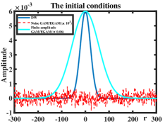
Figure 1: Initial conditions of DW and GAM/EGAM. Others are normalized to the DW initial envelope (blue curve) to have a better view. Here, the blue-green solid line represents the broad mode structure of the EGAM, the blue solid line is the initial envelope of DW, and the red dashed line shows the random distribution of the small amplitude EGAM/GAM.

III Accelerated propagation

Due to the balance of DW kinetic dispersiveness and nonlinear trapping effect of GAM, it is expected and shown numerically in Ref. 11 that, DW and GAM can couple together and propagate in the radial direction consistently with little dispersion in the form of solitons, causing enhanced DW turbulence spreading. Thus, it is naturally interested to find out the effects of the linear EPs drive on the soliton propagation and also the possible existence of cross-scale interaction. In align with the previous work on the spontaneous excitation of GAM by the DW Chen et al. (2021a), we focus on the comparisons between the first and third scenarios above, while the second and forth scenarios will also be discussed briefly.

The initially Gaussian envelope for the DW splits into multiple soliton structures due to the nonlinear coupling to the EGAM, as shown in the Fig. 2a, and the velocity of the solitons are measured by finding the outmost maximums. It is found numerically that propagation of the coupled DW-EGAM solitons is enhanced. As shown in Fig. 3, the position of the maximum of the DW for linear growth rate of EGAM $\gamma_{G}=0$ and $0.03$ are presented, and the velocity for the first and third scenarios are 1.25 and 1.40, respectively. This has an implication for fusion devices, that the existence of linear EPs drive may enhance the turbulence spreading. The lowest order of DW solitons velocity is $V_{d}=2C_{d}k_{r}$ Qiu et al. (2014); Chen et al. (2021a), thus, the observed acceleration might be related to the excitation of higher-$k_{r}$ harmonics. To verify this hypothesis, the $k_{r}$ spectrum and corresponding spatial-temporal evolution of the DW and EGAM are investigated, as demonstrated in Fig. 4 and Fig. 5. It is found that, the $k_{r}$ spectrum of the DW for the third scenario is indeed broader than that for the first scenario, indicating possible relation between the higher-$k_{r}$ DW spectrum and the accelerated propagation. The dependence of the velocity on the dominant $k_{r}$ for the first and third scenarios is not obvious due to the existence of multi-dominant modes, while the dependence is more clear for the second scenario shown in the Fig. 4c, in which the mode with $k_{r}\approx 1.5$ dominates after $t=100$, corresponding to the single soliton propagate at $V_{d}\approx 3$, as demonstrated in the Fig. 2b.

The reason for the excitation of high-$k_{r}$ modes can be analyzed in a local analysis of the frequency/wavenumber matching condition. The matching condition arises from the parametric decay instability Zonca and Chen (2008); Qiu et al. (2014); Chakrabarti et al. (2008), which correspond to the conservation of the energy and momentum, and can be determined by $\mathscr{E}_{dr}(\omega_{r},k_{r})=0$, $\mathscr{E}_{Gr}(\omega_{r},k_{r})=0$ for maximized drive, especially as the two sidebands are linearly damped. In the present case with finite linear $\gamma_{G}$, however, the parametric process is thresholdless, thus, a spectrum of modes centered around resonant $k_{r}\sim 0.32$ can excited, and higher-$k_{r}$ modes with higher growth rates (noting $\gamma\propto k_{r}$ for resonant decay Qiu et al. (2014)) and higher propagation velocity may dominate, as observed in the third scenario. Additionally, the enhancement of the resonant $k_{r}$ is more significant in the second scenario, which is similar to the third scenario, since the growing small amplitude EGAM due to the linear EPs drive lead to the macro-scale large amplitude EGAM. In fact, the second scenario is nearly equivalent to the third scenario with large and transient $\gamma_{G}$, though the overall growth rate for the EGAM shall not exceed its real frequency in this model. The nonlinear term in the equation (5) for the second scenario is so large ($v(r=0,t=0)=0.1$) that the frequency of DW is strongly increased and the matching conditions are given as $\omega+C_{d}k_{r}^{2}=\Gamma_{0}v(r=0,t=0)$ and $-\omega^{2}+\omega_{G}^{2}+C_{G}\omega_{G}^{2}k_{r}^{2}=0$ Qiu et al. (2015); Chen et al. (2021b). The lowest order resonant $k_{r}$ can be derived as $k_{r}=\sqrt{\Gamma_{0}v/C_{d}}$, i.e., $k_{r}=\sqrt{5}$ for the parameters given in the second scenario, which coincides with the numerical result given in the Fig. 4c ($k_{r}\sim 1.5$). Here, the local assumption is also utilized by treating the EGAM as a stationary background given as $v=v(r=0,t=0)=0.1$, thus, the analysis depicts the resonant condition qualitatively; while radial propagation of the envelope is not covered. The second and third scenarios demonstrate that due to the large amplitude EGAM, the matching condition can be altered, resulting in the increased resonant $k_{r}$. As a consequence, the rapid expansion of the DW spectrum and propagation of the DW envelope in the presence of the $\gamma_{G}$ is reasonable.

Besides, since EGAM is excited in micro- and macro-scales simultaneously by DW and EPs, respectively, the cross-scale interaction intermediated by EGAM is also an important topic. It is shown in the Fig. 5a and Fig. 5c that EPs pump energy to the macro-scale and DW to the micro-scale of EGAM. The Fig. 5b and Fig. 5c are the spectrum of the EGAM/GAM normalized by the maximum at the corresponding time, in order to find out the dominant radial wavenumber each time. When the nonlinearity is turned off, the EGAM with $k_{r}\simeq 0$ is excited; while, when the nonlinearity is turned off and in the absence of the linear EPs drive, the EGAM with $k_{r}\simeq 0.32$ is excited, as demonstrated in the Fig. 5c. If both the nonlinear and linear drives exist, as shown in the Fig. 5b, the spectrum of the EGAM seems to be superposition of the former two cases. More precisely, the nonlinearity dominates during $t=100-250$, then the EGAM nonlinearly saturates and the linear EPs drive dominates. Indeed, the interaction between the macro (linear EPs drive) and the micro-scale (nonlinear drive) is relatively weak in this nonlinear system, possibly due to the linear nature of the EPs effect in this work.

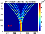
(a)

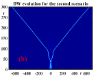
(b)

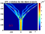
(c)

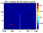
(d)

Figure 2: The spatial-temporal evolution of the DW for the (a) first scenario, (b) second scenario, (c) third scenario and (d) forth scenario. The horizontal axis is the radial scale, and the vertical axis is time.

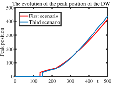
Figure 3: The evolution of the radial position of the DW soliton. The red and blue solid lines represent the peak position of the DW for the first and third scenarios.

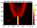
(a)

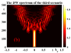
(b)

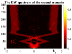
(c)

Figure 4: The evolution of the $k_{r}$ spectrum of the DW for the (a) first, (b)third and (c) second scenarios.

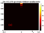
(a)

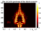
(b)

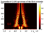
(c)

Figure 5: The evolution of the $k_{r}$ spectrum of the EGAM for (a) nonlinearity turned off, (b) nonlinearity turned on and (c) nonlinearity turned on without the linear EPs drive. The spectrum shown in (b) and (c) are normalized to the maximum at each time step.

IV Conservation laws and energy flow

The conservation laws are significant for describing a nonlinear system. The conservation law can be written as $\rho_{t}+J_{x}=S_{0}$, where $\rho$ is the “density”, $J$ is the corresponding flux, and $S_{0}$ is the source. Assuming that as $x\rightarrow\infty$, $J\rightarrow 0$, then general form of a conserved quantity can be written as

$$\dfrac{d}{dt}\int_{-\infty}^{+\infty}\rho dx = \int_{-\infty}^{+\infty}S_{0}dx.$$ (7)

This expression demonstrates that $\rho$ is conserved in the absence of the source $S_{0}$. In this section, the conservation laws, especially the energy conservation law, of the nonlinear DW-EGAM system will be derived and analyzed to figure out the energy transfer process of the nonlinear system. The first conservation law can be directly derived from the nonlinear evolution equation of DW and it has already been derived in the Ref. Chen et al. (2021a). By adding $u^{*}\times(\ref{eq:DW Eq})$ to its complex conjugate, the conservation law can be written as

$$\left|u\right|_{t}^{2}+iC_{d}\left(u^{*}u_{r}-uu_{r}^{*}\right)_{r} = 0.$$ (8)

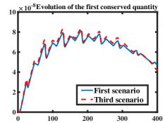
Figure 6: The conservation of the first conserved quantity $W$ is shown here, with the blue solid and red dashed lines representing the temporal evolution of $W$ for the first and third scenarios.

Then, the conserved quantity can be derived by integrating the equation over the whole domain, i.e., $dW/dt=0$, where $W\equiv\left\langle\left|u\right|^{2}\right\rangle$ with $\left\langle\cdots\right\rangle\equiv\int_{-\infty}^{+\infty}\cdots dr$ representing the integration over the whole domain. The conservation of $W$ is demonstrated in Fig. 6, which can also be used to benchmark the numerical scheme. Here, the relative error $(W-W(t=0))/W(t=0)$ is about $10^{-7}$ for the first and third scenarios. The accuracy of $W$ for the second and forth scenarios is also up to $10^{-4}$, though it is much larger than that in the first and third scenario. Based on the first conservation law, equation (6) can be rewritten as

$$v_{tt}-2\gamma_{G}v_{t}+\omega_{G}^{2}v-C_{G}\omega_{G}^{2}v_{rr} = \dfrac{\alpha_{i}\tau\Gamma_{0}}{C_{d}}\left|u\right|_{tt}^{2}.$$ (9)

The coupled equations (5) and (9) are similar to the well-known Zakharov equations. Hence, the energy conservation law can be derived following the standard procedure of the Zakharov system Zarharov (1972). By defining $\phi_{t}\equiv v$, the coupled equations with the form of the conservation laws can be derived by adding $u_{t}^{*}\times(\ref{eq:DW Eq})$ to its complex conjugate and multiplying equation (9) with $\phi$, which can be written as

$$\left[\left|u\right|^{2}+\dfrac{C_{d}}{2}\left(uu_{rr}^{*}+u^{*}u_{rr}\right)\right]_{t}+\dfrac{C_{d}}{2}\left(u_{r}u_{t}^{*}+u_{r}^{*}u_{t}\right.$$

$$\left.-uu_{tr}^{*}-u^{*}u_{tr}\right)_{r}=-\Gamma_{0}v\left|u\right|_{t}^{2},$$ (10)

$$\left(\phi v_{t}-\dfrac{v^{2}}{2}+\dfrac{\omega_{G}^{2}\phi^{2}}{2}+\dfrac{C_{G}\omega_{G}^{2}\phi_{r}^{2}}{2}-2\gamma_{G}\phi v\right)_{t}$$

$$+\left(-C_{G}\omega_{G}^{2}\phi\phi_{rt}\right)_{r}=-\dfrac{\Gamma_{0}\alpha_{i}\tau}{C_{d}}v\left|u\right|_{t}^{2}.$$ (11)

Combining the above equations and integrating over the whole domain, the energy conservation quantity can be obtained

$$\frac{d}{dt}E=\left\langle 2\gamma_{G}v^{2}\right\rangle,$$ (12)

with

$$E\equiv\left\langle-{\phi\phi_{tt}+\dfrac{\lvert\phi_{t}\rvert^{2}}{2}-\dfrac{\omega_{G}^{2}\phi^{2}}{2}-\dfrac{C_{G}\omega_{G}^{2}\lvert\phi_{t}\rvert^{2}}{2}+2\gamma_{G}\phi\phi_{t}}\right.$$

$$\left.{+\dfrac{\alpha_{i}\tau\Gamma_{0}}{C_{d}}\phi\left|u\right|_{t}^{2}}+\alpha_{i}\tau\left({\dfrac{\left|u\right|^{2}}{C_{d}}+\dfrac{\left(u^{*}u_{rr}+uu_{rr}^{*}\right)}{2}}\right)\right\rangle.$$

The terms on the LHS of the E represent the time derivative of the total energy $E$ of the nonlinear system, indicating that the increase of $E$ originates from the linear energy source on the RHS. Thus, in the absence of the linear EPs drive, i.e., in the first and second scenarios, the total energy should be conserved. This is demonstrated in the Fig. 7, where the evolution of the relative error of the total energy $((E-E(t=0))/E(t=0))$ are presented. It is found that the total energy is accurately conserved up to $10^{-6}$. Additionally, for the third and forth scenarios with finite linear EPs drive, the total energy increases exponentially because of the source term on the RHS of the equation (12). Note that, the RHS of equation (12) is proportionate to $\exp(2\gamma_{G0}t)$ through $\left\langle v^{2}\right\rangle$, which can be validated if the slope of $\ln E-t$ diagram is $2\gamma_{G}$. The slope of the total energy logarithm are 0.059 for both scenarios, as shown by the linear fitting in the Fig. 7b, and we can conclude that the total energy $W$ is still conserved accounting for the energy source. Above all, the total energy is accurately conserved for four scenarios investigated here, and this fact establishes a solid foundation for the investigation of energy transfer process.

The ZFs is expected to reduce the turbulence level by the flow shearing Lin et al. (1998); Hahm et al. (1999). Thus, the “deliberate” excitation of the EGAM by the externally injected EPs is proposed as an active control of DW turbulence. However, the “unexpected” excitation of DW turbulence from the Dimits shift region by the EGAM was observed in the gyrokinetic simulation, indicating possible energy transfer from the EGAM to the DW Zarzoso et al. (2013). This unusual result can be understood as an analogy with the le chatelier principle in the chemistry, where the extra introduction of the product, EGAM in this case, would trigger the reverse reaction, i.e., the enhancement of the DW turbulence. Thus, the energy transfer in the nonlinear system is quite an important topic to clarify the controversy. This is accomplished by investigating the evolution of each wave components. The total energy can be decomposed into three components, i.e., $E=E_{G}+E_{D}+E_{I}$, with $E_{G}$ and $E_{D}$ coming from the linear terms of EGAM and DW, respectively, and $E_{I}$ stemming from the nonlinear terms. More specifically, each energy components can be given explicitly as follows

$$E_{G}\equiv\left\langle-\phi\phi_{tt}+\dfrac{\phi_{t}^{2}}{2}-\dfrac{\omega_{G}^{2}\phi^{2}}{2}-\dfrac{C_{G}\omega_{G}^{2}\phi_{x}^{2}}{2}+2\gamma_{G}\phi\phi_{t}\right\rangle,$$

$$E_{D}\equiv\left\langle\alpha_{i}\tau\left(\dfrac{\left|u\right|^{2}}{C_{d}}+\dfrac{\left(u^{*}u_{rr}+uu_{rr}^{*}\right)}{2}\right)\right\rangle,$$

$$E_{I}\equiv\left\langle\dfrac{\alpha_{i}\tau\Gamma_{0}}{C_{d}}\phi\left|u\right|_{t}^{2}\right\rangle.$$

The energy transfer is demonstrated by the evolution of each energy component, i.e., the decrease/increase of an energy component means lose/gain energy from other components. The evolution of each energy component is shown in Fig. 8. The first scenario is presented in Fig. 8a, which corresponds to the spontaneous excitation of the GAM by the DW. It clearly shows the transfer of energy from the DW to the GAM, which coincides with the previous investigations. Fig. 8b shows the evolution of each energy components in the second scenario. It is found that the DW pumps energy into the EGAM as that in the first scenario, with the difference that the interaction energy increases and decreases periodically in this case. The energy transfer process for the third and forth scenario are shown in the Fig. 8c and 8d, both demonstrating the energy transfer from the DW to the EGAM. The energy of the EGAM $E_{G}$ is not shown here, because the exponentially growing $E_{G}$ would dominate $E_{D}$ and $E_{I}$ due to the total energy conservation. In all four scenarios, the DW energy always decreases, showing no energy transfer from GAM/EGAM to DW. Thus, we conclude, in the present model for GAM/EGAM interaction with DW, there is no sign of DW “excitation” by GAM/EGAM, and further investigations are needed to understand the observations of Ref. 26.

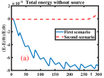
(a)

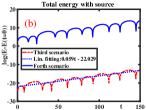
(b)

Figure 7: The evolution of the total energy for the (a) third and (b) forth scenarios is shown here, with the blue solid and red dashed lines in (a) representing the evolution of $E$ for the first and second scenarios. The deep blue solid and red dashed lines in (b) demonstrate the evolution of the logarithm of $E$ for the forth and third scenarios, while, the blue dashed line is the linear fitting.

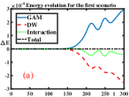
(a)

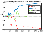
(b)

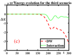
(c)

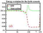
(d)

Figure 8: The evolution of each energy components for the first to forth scenarios. In the first two figures, the blue solid, red dashed, green dashed and the black dashed lines represent the energy variation of the EGAM/GAM, DW, Interaction and total, respectively. The deep-blue solid and red dashed lines in the latter figures represent the evolution of the DW and interaction energy.

V Conclusion and discussion

In this work, we have investigated the nonlinear interaction between ambient DW turbulence and EGAM, by using the first-principle based two-field equations. Four scenarios with different combinations of EGAM/GAM initial amplitude and linear GAM growth rate are designed to delineate the effects of linear drive and finite GAM amplitude Chen et al. (2021b) on DW-EGAM nonlinear interactions Zarzoso et al. (2013), including DW regulation as well as turbulence spreading. The energy conservation law for the nonlinear system is derived and verified numerically. Based on that, the energy transfer between different energy components are analyzed in detail.

Firstly, the propagation of DW-EGAM solitons was investigated. The continuous acceleration of DW-EGAM solitons are observed in the numerical simulation, in which the peak position of the DW is presented. The fact may arise from the excitation of higher $k_{r}$ DWs, i.e., the modes with micro-scale mode structures, due to the modifications of the frequency/wavenumber matching condition by linear EPs drive, resulting in the up-shift of resonant $k_{r}$. Secondly, two conservation laws, including the energy conservation law, are derived following that of the nonlinear Zakharov system. The numerical simulations have proved that the energy is accurately conserved. In addition, the total energy can be decomposed into the energy of the DW, EGAM and interaction, thus, the energy transfer between different modes can be investigated. It is found that DW transfers energy to EGAM in all four different scenarios, aligning with common speculation. This result imply that, in this nonlinear DW-EGAM system, GAM/EGAM stabilizes DW turbulence via the nonlinear energy transfer, as a complement of the previous publications.

Though DW is damped by EGAM nonlinearly, the enhancement of turbulence spreading from the DW linearly stable to unstable region might offset the positive effect of EGAM on plasma confinement. The overall outcome needs further investigation. Moreover, part of the dynamical behaviour of the coupled equations are surveyed numerically in this work, which is a brief dipiction of the complex nonlinear system. Thus, more thorough investigations, especially theoretical treatment, are needed to obtain a better understanding to the nonlinear system. More importantly, little energy exchanges, between the meso-scale GAM and the macro-scale component of EGAM observed in this work, implies that the indirect nonlinear interactions between the Alfvén eigenmodes (AEs) and the DW, mediated by the ZFs, might be relatively weak. Previous works based on the two prey-one predator model, in which the spatial evolution is neglected, could, thus, be incomplete. As a consequence, the direct cross-scale interactions of the AEs and DWs Chen et al. (2022) could be crucial. Finally, as the linear EPs drive may contribute to DW turbulence spreading, the ion diamagnetic frequency nonuniformity $\omega_{*}(r)$, could be more significant in the presence of linear EPs drive, to determine the range of turbulence spreading via rendering the convective nature of DW-GAM system into a quasi-absolute instability, as shown in Ref. Qiu et al. (2014). These aspects will be investigated in a future publication.

Data availability

The data that support the findings of this study are available from the corresponding author upon reasonable request.

References

- Horton (1999) W. Horton, Rev. Mod. Phys. 71, 735 (1999).
- Tomabechi et al. (1991) K. Tomabechi, J. Gilleland, Y. Sokolov, R. Toschi, and I. Team, Nuclear Fusion 31, 1135 (1991).
- Wan et al. (2017) Y. Wan, J. Li, Y. Liu, X. Wang, V. Chan, C. Chen, X. Duan, P. Fu, X. Gao, K. Feng, et al., Nuclear Fusion 57, 102009 (2017).
- Garbet et al. (1994) X. Garbet, L. Laurent, A. Samain, and J. Chinardet, Nuclear Fusion 34, 963 (1994).
- Hahm et al. (2004) T. S. Hahm, P. H. Diamond, Z. Lin, K. Itoh, and S.-I. Itoh, Plasma Physics and Controlled Fusion 46, A323 (2004).
- Hahm et al. (2005) T. S. Hahm, P. H. Diamond, Z. Lin, G. Rewoldt, O. Gurcan, and S. Ethier, Physics of Plasmas 12, 090903 (2005).
- Hasegawa et al. (1979) A. Hasegawa, C. G. Maclennan, and Y. Kodama, Physics of Fluids 22, 2122 (1979).
- Diamond et al. (2005) P. H. Diamond, S.-I. Itoh, K. Itoh, and T. S. Hahm, Plasma Physics and Controlled Fusion 47, R35 (2005).
- Lin et al. (1998) Z. Lin, T. S. Hahm, W. W. Lee, W. M. Tang, and R. B. White, Science 281, 1835 (1998).
- Guo et al. (2009) Z. Guo, L. Chen, and F. Zonca, Phys. Rev. Lett. 103, 055002 (2009).
- Chen et al. (2021a) N. Chen, S. Wei, G. Wei, and Z. Qiu, Plasma Physics and Controlled Fusion 64, 015003 (2021a).
- Rosenbluth and Hinton (1998) M. N. Rosenbluth and F. L. Hinton, Phys. Rev. Lett. 80, 724 (1998).
- Winsor et al. (1968) N. Winsor, J. L. Johnson, and J. M. Dawson, Physics of Fluids 11, 2448 (1968).
- Zonca and Chen (2008) F. Zonca and L. Chen, Europhys. Lett. 83, 35001 (2008).
- Qiu et al. (2018) Z. Qiu, L. Chen, and F. Zonca, Plasma Science and Technology 20, 094004 (2018).
- Conway et al. (2021) G. D. Conway, A. I. Smolyakov, and T. Ido, Nuclear Fusion (2021).
- Chen et al. (2000) L. Chen, Z. Lin, and R. White, Physics of Plasmas 7, 3129 (2000).
- Zhao et al. (2006) K. J. Zhao, T. Lan, J. Q. Dong, L. W. Yan, W. Y. Hong, C. X. Yu, A. D. Liu, J. Qian, J. Cheng, D. L. Yu, et al., Phys. Rev. Lett. 96, 255004 (2006).
- Conway et al. (2008) G. D. Conway, C. Troster, B. Scott, K. Hallatschek, and the ASDEX Upgrade Team, Plasma Physics and Controlled Fusion 50, 055009 (2008).
- Lan et al. (2008) T. Lan, A. D. Liu, C. X. Yu, L. W. Yan, W. Y. Hong, K. J. Zhao, J. Q. Dong, J. Qian, J. Cheng, D. L. Yu, et al., Physics of Plasmas 15, 056105 (2008).
- Zhong et al. (2015) W. Zhong, Z. Shi, Y. Xu, X. Zou, X. Duan, W. Chen, M. Jiang, Z. Yang, B. Zhang, P. Shi, et al., Nuclear Fusion 55, 113005 (2015).
- Melnikov et al. (2017) A. Melnikov, L. Eliseev, S. Lysenko, M. Ufimtsev, and V. Zenin, Nuclear Fusion 57, 115001 (2017).
- Nazikian et al. (2008) R. Nazikian, G. Fu, M. Austin, and et al, Phys. Rev. Lett. 101, 185001 (2008).
- Fu (2008) G. Fu, Phys. Rev. Lett. 101, 185002 (2008).
- Qiu et al. (2010) Z. Qiu, F. Zonca, and L. Chen, Plasma Physics and Controlled Fusion 52, 095003 (2010).
- Zarzoso et al. (2013) D. Zarzoso, Y. Sarazin, X. Garbet, R. Dumont, A. Strugarek, J. Abiteboul, T. Cartier-Michaud, G. Dif-Pradalier, P. Ghendrih, V. Grandgirard, et al., Phys. Rev. Lett. 110, 125002 (2013).
- Chen et al. (2021b) N. Chen, H. Hu, X. Zhang, S. Wei, and Z. Qiu, Physics of Plasmas 28, 042505 (2021b).
- Zonca et al. (2004) F. Zonca, R. B. White, and L. Chen, Physics of Plasmas 11, 2488 (2004).
- Zarharov (1972) V. E. Zarharov, Soviet Physics JETP 35, 908 (1972).
- Frieman and Chen (1982) E. A. Frieman and L. Chen, Physics of Fluids 25, 502 (1982).
- Romanelli and Zonca (1993) F. Romanelli and F. Zonca, Physics of Fluids B 5, - (1993).
- Qiu et al. (2014) Z. Qiu, L. Chen, and F. Zonca, Physics of Plasmas 21, 022304 (2014).
- O’Neil et al. (1971) T. M. O’Neil, J. H. Winfrey, and J. H. Malmberg, The Physics of Fluids 14, 1204 (1971).
- Qiu et al. (2009) Z. Qiu, L. Chen, and F. Zonca, Plasma Physics and Controlled Fusion 51, 012001 (2009).
- Biancalani et al. (2017) A. Biancalani, I. Chavdarovski, Z. Qiu, A. Bottino, D. Del Sarto, A. Ghizzo, O. Gurcan, P. Morel, and I. Novikau, Journal of Plasma Physics 83 (2017).
- Chakrabarti et al. (2008) N. Chakrabarti, P. N. Guzdar, R. G. Kleva, V. Naulin, J. J. Rasmussen, and P. K. Kaw, Physics of Plasmas 15, 112310 (2008).
- Qiu et al. (2015) Z. Qiu, L. Chen, and F. Zonca, Physics of Plasmas 22, 042512 (2015).
- Hahm et al. (1999) T. S. Hahm, M. A. Beer, Z. Lin, G. W. Hammett, W. W. Lee, and W. M. Tang, Physics of Plasmas 6, 922 (1999).
- Chen et al. (2022) L. Chen, Z. Qiu, and F. Zonca, Nuclear Fusion 62, 094001 (2022).