A point process model for rare event detection

Abstract

Detecting rare events, those defined to give rise to high impact but have a low probability of occurring, is a challenge in a number of domains including meteorological, environmental, financial and economic. The use of machine learning to detect such events is becoming increasingly popular, since they offer an effective and scalable solution when compared to traditional signature-based detection methods. In this work, we begin by undertaking exploratory data analysis, and present techniques that can be used in a framework for employing machine learning methods for rare event detection. Strategies to deal with the imbalance of classes including the selection of performance metrics are also discussed. Despite their popularity, we believe the performance of conventional machine learning classifiers could be further improved, since they are agnostic to the natural order over time in which the events occur. Stochastic processes on the other hand, model sequences of events by exploiting their temporal structure such as clustering and dependence between the different types of events. We develop a model for classification based on Hawkes processes and apply it to a dataset of e-commerce transactions, resulting in not only better predictive performance but also deriving inferences regarding the temporal dynamics of the data.

Keywords: imbalanced classification; performance metrics; Hawkes processes

1 Introduction

Many real world applications require the detection of rare observations in large data. For example, intrusions in computer networks (Bhuyan et al., 2013), fraudulent transactions in financial data (Fiore et al., 2019), system failures (Ribeiro et al., 2016) and road accidents in traffic data (Theofilatos et al., 2016) are significant but rare events that require detection. In the literature, such rare events may be referred to as abnormalities, anomalies, novelties, outliers, exceptions, aberrations or contaminations, among others.

Rare event detection is recognised as a very challenging problem. It has become infeasible for investigators to manually detect rare events in real world applications, due to the large number of observations and high dimensionality. As a result, the use of machine learning techniques have become increasingly popular as they offer an effective and scalable solution to automate the process of identifying rare events from large volumes of data. However, due to the inherent imbalance of the classes in such datasets, statistical methods tend to underestimate the probability of rare events and perform poorly (King and Zeng, 2001).

In this paper, we present techniques that build towards a general framework for employing machine learning based models for rare event detection. Using a publicly available dataset of e-commerce transactions, we first illustrate how one can develop a better understanding of such data using a series of visualisations. Strategies to deal with the imbalance of the classes including the crucial selection of performance metrics for evaluating models are also discussed.

Typical machine learning algorithms, however, do not naturally account for the fact that events are ordered in time and, as such, are unable to capture any dependence these events may have on past occurrences. Stochastic processes such as Hawkes processes (Hawkes, 1971), on the other hand, model sequences of events by exploiting their temporal structure such as clustering and dependence between the different types of events. In this paper, we develop a model for classifying events based on Hawkes processes that can be applied to a wide range of applications that generate event data streams.

We evaluate the accuracy of the point process based classifier by comparing against typical ML classifiers and confirm the superior predictive performance of the point process model. We also provide a detailed parameter description showing how the point process model parameters can be used to gain valuable insights into the underlying phenomena that generated the data.

Figure 1: Snapshot of the dataset from the Kaggle competition IEEE-CIS Fraud Detection.

2 Data

To illustrate the methodology developed as part of our work, we use a public dataset containing real world e-commerce transactions made available as part of the Kaggle competition IEEE-CIS Fraud Detection: Can you detect fraud from customer transactions? (Kaggle contributors, 2020). Financial fraud detection is a typical example of rare event detection where the data is often characterised by large number of samples and a severe imbalance in the number fraudulent samples compared to normal ones.

The original dataset contains over 400 variables, however, the vast majority of the variables have their names and values masked for privacy protection. We exclude the masked variables, as is the case in comparable studies, such as (Bhattacharyya et al., 2011; Carneiro et al., 2017), since they offer little value while illustrating the general modelling framework and its interpretability. We retain only nine variables in our reduced dataset including the target variable isFraud which is an indicator of the transaction being fraudulent. Figure 1 is a snapshot of the dataset with the variables included in our analyses.

Figure 2: Distribution of the target isFraud.

(a) Logarithm of the transaction amounts
grouped by isFraud.

(b) Logarithm of the days since last
transaction grouped by isFraud.

Figure 3: Distribution of logarithm of the transaction amounts (left) and the logarithm of the days since the last transaction (right) grouped by isFraud.

(a) isFraud by Card type.

(b) isFraud by Card category.

Figure 4: Mosaic plots showing the distribution of isFraud by various features.

2.1 Exploratory data analysis

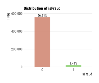
In this section, we explore the dataset through a series of visualisations to get a better understanding of the variables in the data and their distributions. Figure 2 is the distribution of the target variable isFraud, showing the severe imbalance in the proportion of fraudulent to normal transactions.

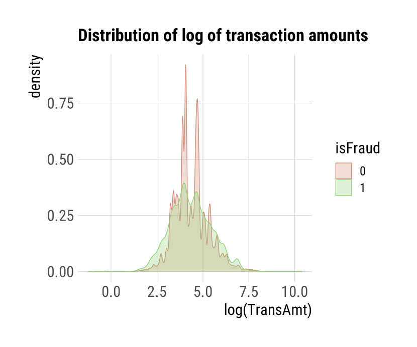
Figure 3(a) is the distribution of the logarithm of the transaction amounts grouped by isFraud, where we observe the fraudulent transactions having a much smoother distribution over the transaction amounts. This could be an indication that fraudsters avoid multiple transactions with the same amount.

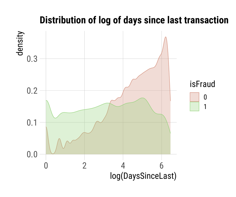
Figure 3(b) is the distribution of the logarithm of the days since the last transaction grouped by isFraud, where we observe that fraudulent transactions are much likely to occur when there has been a previous transaction within the last 14 days. This could indicate that fraudulent activity is likely to cluster in time.

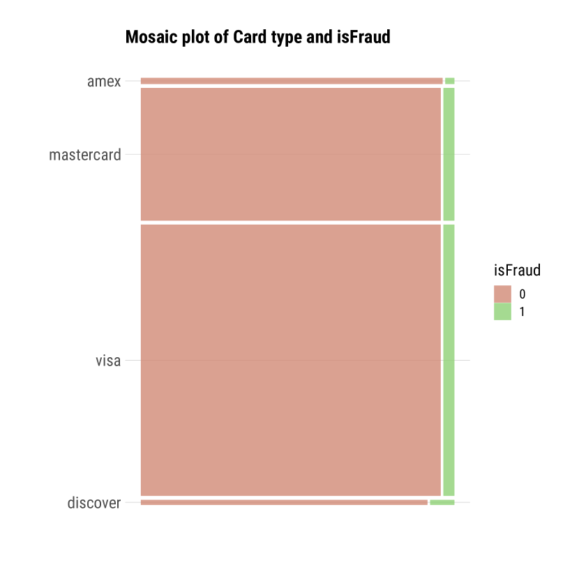
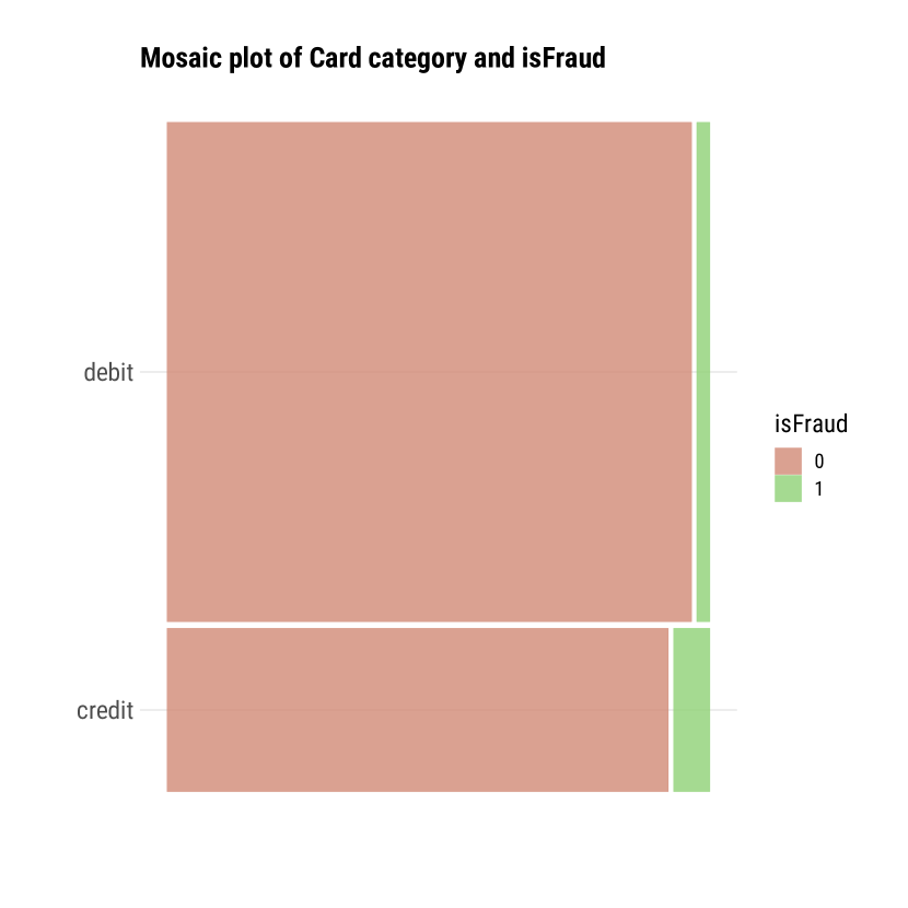
Figures 4(a) and 4(b) are mosaic plots showing the two-dimensional distribution of the target isFraud along with another variable. The variable values along the y-axes are ordered with values having the smallest proportion of fraud at the top to the largest at the bottom. These figures show the distribution of the variable categories as well as help us recognise the categories with large fraud proportions.

3 Related work

As mentioned earlier, detecting fraudulent financial transactions is a typical example of classifying rare events, that is characterised by large volumes of data and a severe imbalance of the classes. A systematic review of 49 articles using supervised machine learning approaches for fraud detection in Ngai et al. (2011) showed that Logistic Regression, Decision Trees, Neural Networks and Support Vector Machines are among the popular methods of choice. Bhattacharyya et al. (2011) did a comparative study of various ML methods for fraud detection under varying proportions of fraud during training and report that Random Forests achieved an overall higher precision at low recall levels. While most fraud detection techniques have been specifically applied to the case of credit-card fraud, Carneiro et al. (2017) is one of the few studies that have examined this problem in an e-commerce dataset. Carneiro et al. (2017) not only develop an automatic system for fraud detection, but also provide insights to fraud analysts for improving their manual revision process, which resulted in an overall superior performance.

Jensen (1997) studied the technical issues in problems like fraud detection and identified the severe imbalance of the classes as a key challenge. Under-sampling is a strategy to tackle the imbalance problem by removing some instances of the majority class in the training set (Akbani et al., 2004), under the assumption that there is redundancy in the data. Random over-sampling is another strategy where instances of the minority class are replicated (He and Garcia, 2009), but its performance is limited as it does not add any new information. A more successful approach to oversample the minority class is the Synthetic Minority Oversampling Technique (SMOTE) (Chawla et al., 2002), where synthetic examples are generated by interpolating between examples of the minority class.

The selection of an appropriate performance metric is key in imbalanced classification problems and it is well-known that measures like Accuracy, True Positive Rate and True Negative Rate can be misleading (Provost, 2000). As a result, most literature often rely on the area under the ROC curve (Dal Pozzolo et al., 2014), but this ignores the fact that the performance on the minority class is more important for businesses.

Almost all methods in the literature for fraud detection do not naturally account for the fact that events are ordered in time and hence may depend on past occurrences. To the best of our knowledge, the development of a classifier based on point processes that model sequences of events by exploiting their temporal structure is novel.

4 Supervised machine learning approach

We focus on supervised machine learning methods for rare event detection tasks like fraud detection, that can be broken down into two steps. The first step of supervised learning consists of building a prediction model from a set of labelled (‘normal’ or ‘fraudulent’) historical data. In the second step, the prediction model obtained from the supervised learning process is used to predict the label of new transactions.

Formally, a prediction model is a parametric function with parameters $\theta$ that takes an input $x$ from an input space $\mathcal{X}\in\mathbb{R}^{n}$, and outputs a prediction $\hat{y}=p(x,\theta)$ over an output space $\mathcal{Y}\in\mathbb{R}$.

The input space $\mathcal{X}$ usually differs from the space of raw transaction data as most supervised learning algorithms require the input domain to be real-valued, and therefore may require the transformation of transaction features that are not real numbers (such as timestamps, categorical variables, etc). It may also be beneficial to perform feature engineering to enrich the transaction data to improve the detection performance.

For fraud detection, the output space $\mathcal{Y}$ is usually the predicted binary class for a given input $x$, that is $\mathcal{Y}=\{0,1\}$. Alternatively, the output may also be expressed as a fraud probability, with $\mathcal{Y}=[0,1]$, where values closer to 1 express higher probability of fraud.

The training of a prediction model $p(x,\theta)$ consists of finding the parameters $\theta$ that minimises a loss function, that compares the true label $y$ to the predicted label $\hat{y}=p(x,\theta)$ for an input $x$. Due to the high class imbalance (much more ‘normal’ than ‘fraudulent’ transactions), careful consideration must be given to the choice of loss function for fraud detection. Particular care must also be taken in practice when splitting the dataset into training and validation sets, due to the sequential nature of transactions.

4.1 Tackling class imbalance

The challenge of working with imbalanced datasets is that most machine learning algorithms will ignore, and in turn have poor performance on, the minority class. However, in most cases and particularly for rare event detection, it is the performance on the minority class that is most important. The popular approaches for tacking class imbalance are based on sampling and rely one or both of the following techniques:

1. Over-sampling, by adding more examples of the minority class so it has more effect on the machine learning algorithm. In over-sampling, instead of creating exact copies of the minority class examples, we can introduce small variations into those copies, creating more diverse synthetic samples.

2. Under-sampling, by removing some examples of the majority class so it has less effect on the machine learning algorithm. In under-sampling we can cluster the examples of the majority class, and do the under-sampling by removing examples from each cluster, thus seeking to preserve information.

Figure 5: The absolute difference of the mutual information (MI) between transactions grouped by isFraud before (left) and after (right) applying the SMOTE technique to balance the classes. The absolute differences of MI are higher after SMOTE indicating that the pairwise feature relationships are more distinct between the two classes after balancing.

Figure 6: Dimensionality reduction using t-SNE before (left) and after (right) using SMOTE to balance the classes. The classes appear to be more separable after the application of SMOTE.

4.1.1 SMOTE: Synthetic Minority Over-Sampling Technique

An effective over-sampling technique where new examples are synthesised from the existing examples by introducing small variations is the Synthetic Minority Oversampling Technique (Chawla et al., 2002), or SMOTE for short.

SMOTE works by selecting examples that are close in the feature space, drawing a line between the examples in the feature space and creating a new sample at a point along that line. Specifically, a random example from the minority class is first chosen. Then k of the nearest neighbours for that example are found (typically k=5). A randomly selected neighbour is chosen and a synthetic example is created at a randomly selected point between the two examples in feature space.

The approach is effective because new synthetic examples from the minority class are created that are plausible as they are relatively close in feature space to existing examples from the minority class. A general downside of the approach is that synthetic examples are created without considering the majority class, possibly resulting in ambiguous examples if there is a strong overlap for the classes.

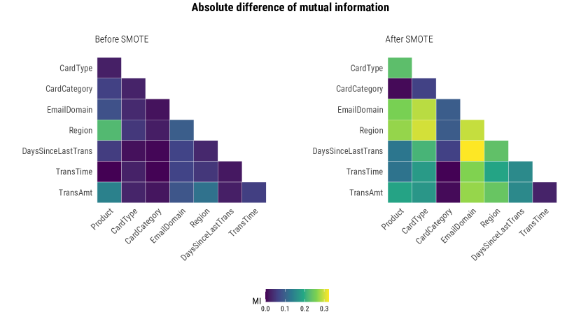
We apply SMOTE to balance the classes in our dataset and assess its impact in the following ways. Figure 5 gives the absolute difference of the mutual information (MI) among all pairs of features between transactions grouped by the target isFraud. The results are shown before (top) and after (bottom) the application of SMOTE. The absolute differences of MI are comparatively higher after SMOTE indicating that the pairwise feature relationships are more distinct between the two classes after balancing.

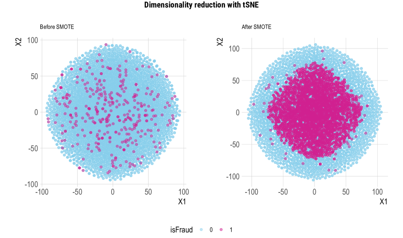
A popular method for exploring high-dimensional data is t-SNE, introduced by Maaten and Hinton (2008), an unsupervised and non-linear dimensionality reduction technique. Figure 6 gives the results of applying t-SNE to visualise the dataset in a reduced two-dimensional space both before (top) and after (bottom) using SMOTE to balance the classes. The classes appear to be relatively more separable after the application of SMOTE.

Table 1: Performance metrics from the modelling experiment before using SMOTE.

Model	Accuracy	ROC_AUC	PR_AUC
Logistic Regression	0.9582	0.7795	0.1905
Bagged Decision Trees	0.9524	0.6661	0.1281

Table 2: Performance metrics from the modelling experiment after using SMOTE.

Model	Accuracy	ROC_AUC	PR_AUC
Logistic Regression	0.8746	0.7866	0.1898
Bagged Decision Trees	0.9527	0.6819	0.1358

4.1.2 Choosing the right metric for imbalanced classification

Selecting an evaluation metric is an important step in any project. Choosing the wrong metric can mean choosing a model that solves a different problem from the problem we actually want solved.

The metric must capture those characteristics about a model and its predictions that are most important to the project stakeholders. This is challenging, as there are many metrics to choose from and often project stakeholders are not sure what they want. Based on whether the positive (minority) class is more important, we make the following recommendations for choosing a metric;

1. Positive class is more important

   • If both false positives and false negatives are equally important, then use the area under the precision recall curve (PR AUC). This maximises both precision and recall over all possible thresholds.

   • If false negatives are more costly, then use the F(2) measure.

   • If false positives are more costly, then use the F(0.5) measure.

2. Both classes are equally important

   • Use the area under the ROC curve (ROC AUC). This maximises the true positive rate and minimises the false positive rate over all possible thresholds.

where the F($\beta$) measure is defined as

$$F(\beta)=\frac{(1+\beta^{2})*\text{precision}*\text{recall}}{\beta^{2}*\text{precision}*\text{recall}}\,.$$

Tables 1 and 2 present the performance metrics of the machine learning algorithms, logistic regression (Kleinbaum et al., 2002) and bagged decision tree (Breiman, 1996), for the fraud classification task both before and after using SMOTE to balance the classes. We use the first 14 days of transactions to train the models and the subsequent 14 days are used for evaluation. Based on these results it appears that class balancing using SMOTE does not provide a significant advantage in classifying fraudulent transactions in this dataset.

Despite the rising popularity of machine learning for rare event detection, a key limitation suffered by most off-the-shelf machine learning methods is that they ignore the natural order in which the events occur over time. As it is reasonable to suspect that transactions could be dependent on past transactions within the sequence, we explore the idea of building a rare event classifier based on point processes.

5 Point process approach

The vast majority of machine learning algorithms, with the exception of recurrent neural networks, are not designed to model event sequences that may have a dependence on past occurrences. In an attempt to overcome this limitation, most people resort to clever feature engineering using the event timestamp, the success of which is heavily reliant on domain expertise as well as the complexity of the underlying phenomena. Point processes on the other hand, model sequences of events by exploiting their temporal structure like clustering and dependence between the different types of events. Such models have the potential to not only offer better predictive performance when compared to conventional ML classifiers but also provide inferences about the temporal dynamics of the data.

Point processes are used to describe a random collection of points in any general space, however, we limit ourselves to the case in which the points denote events that occur along a time axis. Such temporal point processes are well studied (see, for example, Daley and Vere-Jones, 2003) and are suitable for a wide range of real-world applications.

Multivariate point processes are those in which two or more types of points are observed and are specified by associating a random variable, say $m$ denoting the point type. If $m$ is allowed to be a general random variable, then we refer to $m$ as a mark and the process as a marked point process. An example of a marked point process with continuous marks is in seismology, where the magnitude of an earthquake is recorded in addition to the time of occurrence. In this paper, we model sequences of financial transactions using marked point processes with discrete marks used to denote whether the transaction is fraudulent or not.

A popular point process model, the Hawkes process, is a mathematical model for self-exciting processes proposed in Hawkes (1971) that can be used to model a sequence of events of some type over time, for example, earthquakes. Each event excites the process in the sense that the chance of a subsequent event increases for a period of time after the initial event and the excitation from previous events add up. The marked Hawkes process model captures the magnitudes of all cross-excitations between the various event types as well as the rate at which these excitations decay over time. Marked Hawkes processes are specified using a joint conditional intensity function for the occurrence times and the marks (see, for example, Rasmussen, 2013, expression 2.2).

The joint modelling of the times and the marks in a marked point process model has to be decoupled, as we are only interested in predicting the event type (mark) in our classification model. The joint conditional intensity function of a marked point process can be factorised into a conditional intensity function of the occurrences times and a conditional probability mass function for the event mark. Narayanan et al. (2021) showed that the conditional distribution function for the marks can therefore be derived from the joint specification of a marked point process model, resulting in the classification model we are interested in.

(a) Timeline of transactions with isFraud
indicator.

(b) Inter-arrival times between transactions
over the first week.

(c) Boxplot of transaction counts over the 48 consecutive 30 minute windows over each day.

Figure 7: Exploring the temporal dynamics of the transaction data.

Figure 8: Comparing the cumulative distribution functions (CDFs) of the inter-arrival times of events simulated from a Poisson process (red), a Hawkes process (blue), observed event times of the fraudulent transactions.

5.1 Exploring temporal dynamics

The aim here is to investigate the temporal patterns of transactions using the theory of point processes. Each transaction is treated as an event (point) in the process and the isFraud attribute is the event type (mark). The sequence of transactions in the data are therefore represented as a marked point process.

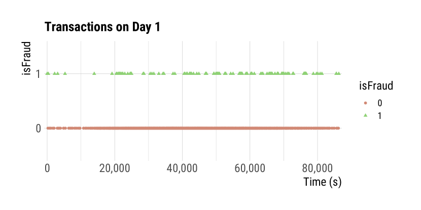
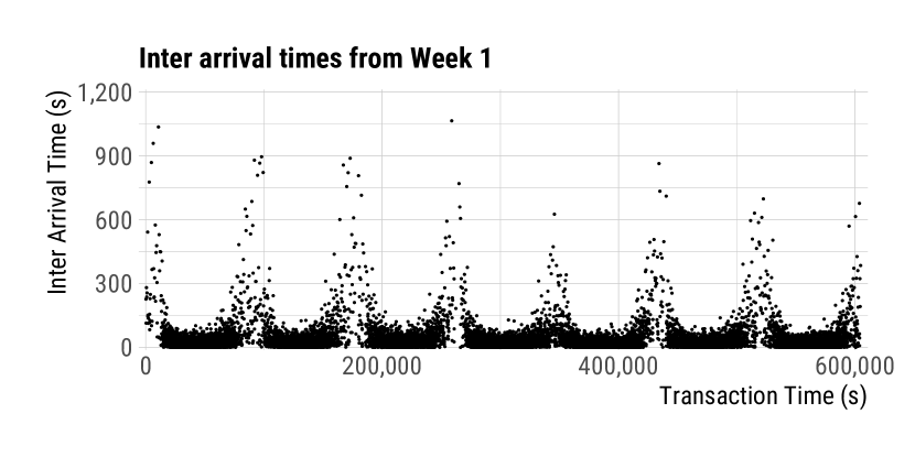
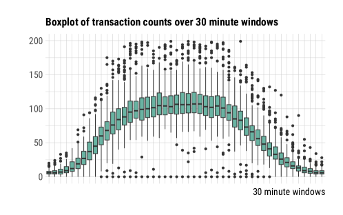
Figure 7(a) shows the timeline of transactions with isFraud indicator over a single day in the dataset. There is a slight indication that fraudulent transactions tend to cluster together. Figure 7(b) plots the inter-arrival times between transactions over the first week, showing a daily seasonality with large inter-arrival times in the early and late hours of the day. To further investigate the daily seasonality, in Figure 7(c), we create a boxplot of transaction counts over the 48 consecutive 30 minute windows that constitute each day in the dataset. Figure 7(c) captures the clear pattern in the frequency of transactions during the course of a day.

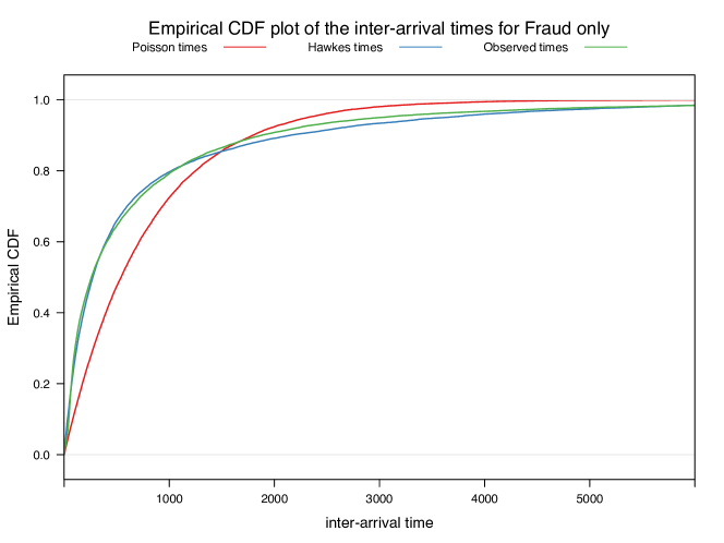
A visual inspection of the occurrence times of fraudulent transactions in Figure 7(a) offered a slight indication that fraudulent transactions may tend to cluster together. To concretely examine if the occurrence of a fraudulent transaction increases the probability of more fraudulent events to occur soon after, we plot the empirical distribution function of the inter-arrival times of the observed fraudulent transactions in Figure 8. We also plot the cumulative distribution functions of a homogeneous Poisson process and an unmarked Hawkes process, whose parameters are estimated from the observed fraudulent events using maximum likelihood. The fitted Poisson process, which is memory-less, is far from the empirical distribution function, while the fitted Hawkes process provides an excellent fit to the observed inter-arrival times. This confirms that the arrival times of fraudulent transactions do depend on past occurrences.

6 Marked point processes

6.1 Conditional intensity function

The collection of the times $\{t_{i}\}$ at which the events occur and the marks $\{m_{i}\}$ is a marked point process, whose ground process, is the process for $\{t_{i}\}$ only. A marked point process is typically specified through its joint conditional intensity function

$$\lambda^{*}(t,m)=\lambda^{*}_{g}(t)f^{*}(m\mid t)\,,$$ (1)

where $\lambda^{*}_{g}(t)$ is the conditional intensity of the ground process and $f^{*}(m\mid t)$ is the conditional probability density or mass function of the mark $m$ at time $t$. Both $\lambda^{*}_{g}(t)$ and $f^{*}(m\mid t)$ in Equation 1 are understood as being conditional on $\mathcal{F}_{t^{-}}$, which is the filtration of the marked point process up to but not including $t$.

6.2 Marked Hawkes processes

Marked Hawkes processes are point processes whose defining characteristic is that they self-excite, meaning that each arrival increases the rate of future arrivals for a period of time. More formally, consider a realisation of a marked point process, consisting of event times $\{t_{i}\}$ with $t_{i}\in\mathbb{R}^{+}$ and $t_{i}>t_{i-1}$, and marks $m_{i}\in\{1,\ldots,M\}$ $(i=1,\dots,n)$, where $M$ is the number of discrete marks. The marked Hawkes process is most intuitively specified using its mark dependent conditional intensity function $\lambda^{*}(t,m)$, which for an exponentially decaying intensity is (Rasmussen, 2013, expression 2.2),

$$\lambda^{*}(t,m)=\mu\delta_{m}+\sum_{t_{j}<t}\alpha\beta\mathrm{e}^{-\beta(t-t_{j})}\gamma_{m_{j}\to m}\,.$$ (2)

In Equation 2, the parameter $\mu>0$ is a constant background intensity and $\delta_{m}\in(0,1)$ is the background mark probability for mark $m$ with $\sum_{m=1}^{M}\delta_{m}=1$. The parameter $\alpha\in(0,1)$ is the excitation factor, $\beta>0$ is the exponential decay rate and $\gamma_{m_{j}\to m}\in(0,1)$ is the probability the excitation from an event of mark $m_{j}$ triggers an event of mark $m$, with $\sum_{m=1}^{M}\gamma_{m_{j}\to m}=1$ for any $m_{j}\in\{1,\ldots,M\}$.

6.3 Deriving the classification model

The conditional probability distribution function of the marks $f(m_{i}\mid t_{i},\mathcal{F}_{t_{i-1}};\boldsymbol{\theta})$, where $\boldsymbol{\theta}$ is an unknown parameter vector, is the classification model we wish to use. As shown in Narayanan et al. (2021), $f(m_{i}\mid t_{i},\mathcal{F}_{t_{i-1}};\boldsymbol{\theta})$ can be derived from the joint conditional intensity function of the marked Hawkes process model in Equation 2 as follows.

By the definition of the conditional intensity function for a marked point process in Equation 1, $f(m_{i}\mid t_{i},\mathcal{F}_{t_{i-1}};\boldsymbol{\theta})=\lambda^{*}(t_{i},m_{i})/\sum_{m=1}^{M}\lambda^{*}(t_{i},m)$. Plugging in $\lambda^{*}(t_{i},m)$ from Equation 2 in the latter expression, gives

$$f(m_{i}\mid t_{i},\mathcal{F}_{t_{i-1}};\boldsymbol{\theta})=\frac{\delta_{m_{i}}+\sum_{t_{j}<t_{i}}\alpha^{*}\mathrm{e}^{-\beta(t_{i}-t_{j})}\gamma_{m_{j}\to m_{i}}}{1+\sum_{t_{j}<t_{i}}\alpha^{*}\mathrm{e}^{-\beta(t_{i}-t_{j})}}\,,$$ (3)

where $\alpha^{*}=\frac{\alpha\beta}{\mu}$. The parameters $\mu$ and $\alpha$ of the marked Hawkes process as specified by Equation 2 are not identifiable. Apart from a mathematical fact, this is also rather intuitive, because $\mu$ and $\alpha$ in Equation 2 characterise the evolution of the Hawkes process in the time dimension and the sequence of marks is not sufficient to identify them.

6.4 Parameter interpretation

In Equation 3, the mark probability of each event in the sequence is determined by a combined additive effect from a background component and all previous occurrences. The first term $\delta_{m_{i}}\in(0,1)$ in the numerator is the probability an event has a mark $m_{i}$ if the event is triggered solely by the background component. Each term $\alpha^{*}\mathrm{e}^{-\beta(t_{i}-t_{j})}\gamma_{m_{j}\to m_{i}}$ is the contribution from a previous occurrence in the sequence while the excitation factor $\alpha^{*}\geq 0$ is a scaling factor applied to the contributions from the previous occurrences. Large values of $\alpha^{*}$ indicate a stronger dependence of the process on its history, since the contributions from previous occurrences are weighted higher relative to the background component. The decay rate $\beta>0$ is the exponential rate at which the excitations from previous occurrences decay over time. The parameter $\gamma_{m_{j}\to m_{i}}\in(0,1)$ is the probability the excitation from an event of mark $m_{j}$ triggers an event of mark $m_{i}$. In other words, $\gamma_{m_{j}\to m_{i}}$ can be viewed as the conversion rate for the transition from an event with mark $m_{j}$ to an event with mark $m_{i}$.

In summary, as in marked Hawkes processes, the specification for the marks in Equation 3 captures not only all cross-excitations between the various marks but also the rate at which these excitations decay over time.

6.5 Including covariates

Transaction datasets in finance and other related sectors, typically carry additional covariates apart from the occurrence times and the indicator variable for fraud. In such cases, we can allow the background mark probability $\boldsymbol{\delta}$ and event conversion rates $\boldsymbol{\gamma}$ to depend on the covariate as

$$f(m_{i}\mid t_{i},z_{i},\mathcal{F}_{t_{i-1}};\boldsymbol{\theta})=\frac{\delta_{m_{i}\mid z_{i}}+\sum_{t_{j}<t_{i}}\alpha^{*}\mathrm{e}^{-\beta(t_{i}-t_{j})}\gamma_{m_{j}\to m_{i}\mid z_{i}}}{\sum_{m=1}^{M}\left[{\delta_{m\mid z_{i}}+\sum_{t_{j}<t_{i}}\alpha^{*}\mathrm{e}^{-\beta(t_{i}-t_{j})}\gamma_{m_{j}\to m\mid z_{i}}}\right]}\,.$$ (4)

where $\{z_{i}\}$ is the collection of the covariate component of the process and the filtration $\mathcal{F}_{t_{i}}$ now includes all times, marks and covariates up to time $t_{i}$.

Table 3: Aggregated counts of event types over each of the 14 days in the training dataset. ‘Normal’ transactions are coded as (mark $=$ 1) and ‘fraudulent’ ones coded as (mark $=$ 2).

day	mark = 1	mark = 2
1	2462	111
2	2235	86
3	2684	127
4	2819	99
5	2900	117
6	2838	141
7	3131	148

day	mark = 1	mark = 2
8	2409	152
9	2283	95
10	2846	78
11	2581	116
12	2671	105
13	2557	118
14	3156	142

7 Results

We use the specification in Equation 4 as the model that classifies the transactions in our dataset as ‘normal’ or ‘fraudulent’. We use only three out of the nine variables from the dataset as shown in Figure 1, namely the TransTime variable as the time dimension, the Product variable as the covariate and the isFraud indicator as the mark dimension.

Table 3 shows the aggregated counts of event types over each of the 14 days that constitute the training dataset. ‘Normal’ transactions are coded as (mark $=$ 1) and ‘fraudulent’ ones coded as (mark $=$ 2). The five types of products are also encoded as integers from 1 to 5.

Table 4: Maximum likelihood estimates with 95% CI.

parameter	value	lower	upper
$\delta_{1\mid 1}$	0.5498	0.3161	0.7635
$\delta_{1\mid 2}$	0.2790	0.0326	0.8161
$\delta_{1\mid 3}$	0.6599	0.2521	0.9179
$\delta_{1\mid 4}$	1.0000	1.0000	1.0000
$\delta_{1\mid 5}$	0.9438	0.8954	0.9705
$\alpha$	3.7011	1.6297	8.4051
$\beta$	0.2649	0.2146	0.3269

parameter	value	lower	upper
$\gamma_{1\to 1\mid 1}$	0.9308	0.9159	0.9432
$\gamma_{2\to 1\mid 1}$	0.0000	0.0000	0.0000
$\gamma_{1\to 1\mid 2}$	0.9466	0.9204	0.9645
$\gamma_{2\to 1\mid 2}$	0.2661	0.0714	0.6309
$\gamma_{1\to 1\mid 3}$	0.9538	0.9337	0.9680
$\gamma_{2\to 1\mid 3}$	0.0000	0.0000	0.0000
$\gamma_{1\to 1\mid 4}$	0.9422	0.9160	0.9606
$\gamma_{2\to 1\mid 4}$	0.0000	0.0000	0.0000
$\gamma_{1\to 1\mid 5}$	0.9860	0.9840	0.9878
$\gamma_{2\to 1\mid 5}$	0.9348	0.8945	0.9604

Table 4 gives the parameter estimates including their 95% confidence intervals after performing parameter estimation using maximum likelihood. The excitation factor $\alpha$ in Equation 4 is a scaling factor applied to the contributions from the previous occurrences to the event mark probability. In Equation 4, the background component has a weight of 1, while previous occurrences are weighted by $\alpha$. The 95% confidence interval for $\alpha$ is $(1.63,8.41)$, meaning the contributions from previous occurrences carry higher weight relative to the background component. In other words, this indicates that financial transactions have a significant dependence on their history.

The decay rate $\beta$ is the exponential rate at which the excitations from previous occurrences decay over time. The 95% confidence interval for $\beta$ is $(0.21,0.33)$, meaning the excitation effect caused by an event lasts for at least 44 minutes after its occurrence before decaying (contribution drops less than $10^{-6}$).

The background mark probability $\delta_{m\mid z}$ in Table 4 is the probability an event with covariate $z$ has a mark $m$ if the event is triggered solely by the background component. An interesting case is of that of product code 4 where the background probability for a fraudulent transaction is nearly 0. In other words, if a fraudulent transaction occurs with product code 4 it has to be necessarily triggered by one of the past occurrences.

Table 5: Maximum likelihood estimates of the triggering probabilities.

product	$\gamma_{r\to c}$	1	2
1	1	0.9308	0.0692
1	2	0.0000	1.0000
2	1	0.9466	0.0534
2	2	0.2661	0.7339
3	1	0.9538	0.0462
3	2	0.0000	1.0000
4	1	0.9422	0.0578
4	2	0.0000	1.0000
5	1	0.9860	0.0140
5	2	0.9348	0.0652

The triggering probability $\gamma_{r\to c}$ in Table 5 is the probability the excitation from an event of mark $r$ triggers an event of mark $c$. The diagonal elements of the $\gamma$ matrix are close to 1 for all products with the exception of product code 5, indicating that events almost exclusively trigger more events of the same type. In other words, for example, the occurrence of a fraudulent event is highly likely to trigger another fraudulent event as compared to a normal event.

In summary, the parameters of the model provide valuable insight into the underlying processes that generated the data. Specifically, we learned how strongly financial transactions depend on their history, the range or duration over which the effects of past events persist as well as the magnitude of cross-excitations that capture the dependence between the different types of events.

Figure 9: Area under the Presicion-Recall Curve.

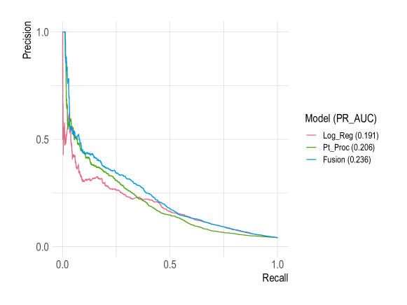
Figure 9 evaluates the predictive performance of the point process based model on the test set which contains transactions over the 14 days immediately after the training data. We use the area under the Presicion-Recall curve as the metric for evaluation, which treats the positive class (fraudulent) as more important and weights both false positives and false negatives equally as discussed in section 4.1.2. We also include the logistic regression model from Table 1 for comparison, which is a typical example of an ML algorithm that does not capture temporal dependence, and we see that the point process model indeed performs better.

8 Conclusions

The performance of the point process model is remarkable despite using just two features from the dataset, namely, the occurrence times and the product covariate, to classify transactions as normal or fraudulent. In contrast, the logistic regression model uses all of the eight features available in the data shown in Figure 1. We also present a fusion model in Figure 9, derived by averaging the predicted probabilities from the two fitted models, in an attempt to combine their arguably different strengths. The fusion model does perform better than either of the models and the fact that even such a naive fusion works well suggests that the two models presented indeed capture very different patterns in the data.

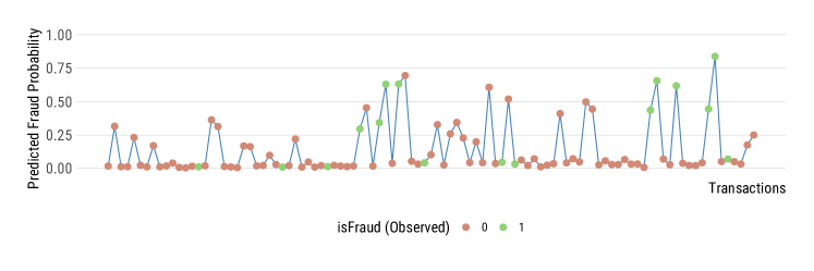
In Figure 10 we show a timeline of predicted fraud probabilities from the point process model, for the first 100 transactions in the test set, to demonstrate how such models can be used in practise. As expected, the model with excitation effects is able to capture the noticeable clustering of fraudulent transactions.

None of the methodology used in our analyses have been tailored specifically for fraud detection or even rare event detection for that matter. Hence, they can be applied to a wide range of applications that generate event data streams.

Figure 10: Timeline of predicted fraud probabilities of the first 100 transactions in the test set.

References

- Akbani et al. (2004) Akbani, R., S. Kwek, and N. Japkowicz (2004). Applying support vector machines to imbalanced datasets. In European conference on machine learning, pp. 39–50. Springer.
- Bhattacharyya et al. (2011) Bhattacharyya, S., S. Jha, K. Tharakunnel, and J. C. Westland (2011). Data mining for credit card fraud: A comparative study. Decision support systems 50(3), 602–613.
- Bhuyan et al. (2013) Bhuyan, M. H., D. K. Bhattacharyya, and J. K. Kalita (2013). Network anomaly detection: methods, systems and tools. Ieee communications surveys & tutorials 16(1), 303–336.
- Breiman (1996) Breiman, L. (1996). Bagging predictors. Machine learning 24(2), 123–140.
- Carneiro et al. (2017) Carneiro, N., G. Figueira, and M. Costa (2017). A data mining based system for credit-card fraud detection in e-tail. Decision Support Systems 95, 91–101.
- Chawla et al. (2002) Chawla, N. V., K. W. Bowyer, L. O. Hall, and W. P. Kegelmeyer (2002). Smote: synthetic minority over-sampling technique. Journal of artificial intelligence research 16, 321–357.
- Dal Pozzolo et al. (2014) Dal Pozzolo, A., O. Caelen, Y.-A. Le Borgne, S. Waterschoot, and G. Bontempi (2014). Learned lessons in credit card fraud detection from a practitioner perspective. Expert systems with applications 41(10), 4915–4928.
- Daley and Vere-Jones (2003) Daley, D. J. and D. Vere-Jones (2003). An introduction to the theory of point processes. Vol. I (2nd ed.). New York: Springer-Verlag.
- Fiore et al. (2019) Fiore, U., A. De Santis, F. Perla, P. Zanetti, and F. Palmieri (2019). Using generative adversarial networks for improving classification effectiveness in credit card fraud detection. Information Sciences 479, 448–455.
- Hawkes (1971) Hawkes, A. G. (1971). Spectra of some self-exciting and mutually exciting point processes. Biometrika 58(1), 83–90.
- He and Garcia (2009) He, H. and E. A. Garcia (2009). Learning from imbalanced data. IEEE Transactions on knowledge and data engineering 21(9), 1263–1284.
- Jensen (1997) Jensen, D. (1997). Prospective assessment of ai technologies for fraud detection: A case study. In AAAI Workshop on AI Approaches to Fraud Detection and Risk Management, pp. 34–38. Citeseer.
- Kaggle contributors (2020) Kaggle contributors (2020). Ieee-cis fraud detection. www.kaggle.com/c/ieee-fraud-detection/data.
- King and Zeng (2001) King, G. and L. Zeng (2001). Logistic regression in rare events data. Political analysis 9(2), 137–163.
- Kleinbaum et al. (2002) Kleinbaum, D. G., K. Dietz, M. Gail, M. Klein, and M. Klein (2002). Logistic regression. Springer.
- Maaten and Hinton (2008) Maaten, L. v. d. and G. Hinton (2008). Visualizing data using t-sne. Journal of machine learning research 9(Nov), 2579–2605.
- Narayanan et al. (2021) Narayanan, S., I. Kosmidis, and P. Dellaportas (2021). Flexible marked spatio-temporal point processes with applications to event sequences from association football. arXiv preprint arXiv:2103.04647.
- Ngai et al. (2011) Ngai, E. W., Y. Hu, Y. H. Wong, Y. Chen, and X. Sun (2011). The application of data mining techniques in financial fraud detection: A classification framework and an academic review of literature. Decision support systems 50(3), 559–569.
- Provost (2000) Provost, F. (2000). Machine learning from imbalanced data sets 101. In Proceedings of the AAAI’2000 workshop on imbalanced data sets, Volume 68, pp. 1–3. AAAI Press.
- Rasmussen (2013) Rasmussen, J. G. (2013). Bayesian inference for hawkes processes. Methodology and Computing in Applied Probability 15(3), 623–642.
- Ribeiro et al. (2016) Ribeiro, R. P., P. Pereira, and J. Gama (2016). Sequential anomalies: a study in the railway industry. Machine Learning 105(1), 127–153.
- Theofilatos et al. (2016) Theofilatos, A., G. Yannis, P. Kopelias, and F. Papadimitriou (2016). Predicting road accidents: a rare-events modeling approach. Transportation research procedia 14, 3399–3405.