Sub-system self-consistency in coupled cluster theory

Abstract

In this Communication, we provide numerical evidence indicating that the single-reference coupled-cluster (CC) energies can be calculated alternatively to its copybook definition. We demonstrate that the CC energy can be reconstructed by diagonalizing the effective Hamiltonians describing correlated sub-systems of the many-body system. In the extreme case, we provide numerical evidences that the CC energy can be reproduced through the diagonalization of the effective Hamiltonian describing sub-system composed of a single electron. These properties of the CC formalism can be exploited to design protocols to define effective interactions in sub-systems used as probes to calculate the energy of the entire system and introduce a new type of self-consistency for approximate CC approaches.

I Introduction

The standard single-reference coupled cluster (SR-CC) theory [1, 2, 3, 4, 5, 6, 7, 8, 9, 10] is a direct consequence of the linked cluster theorem (LCT) and represents the simplest case of exponential Ansatz for the ground-state wave functions. Various SR-CC formulations have been widely used in many areas of physics and chemistry to describe systems and processes driven by complex correlation effects. [11, 12, 13, 14, 15, 16, 17, 18, 19, 20, 21, 22, 23, 24, 25, 26]

Recently, the LCT has been generalized to the active spaces formulations using sub-system embedding sub-algebras CC formalism (SES-CC),[27, 28] which led to new alternative ways for calculating CC energy and allowing one to interpret CC theory as a renormalization (downfolding) procedure. From this point of view, the SR-CC theory can be viewed as a renormalization procedure or rigorous embedding algorithm. The SES-CC formalism or closely related double unitary CC formulations have already inspired several developments to describe strongly correlated systems [29, 30, 31] and time-evolution of quantum systems.[32] (see also Refs.33, 34, 35, 36, 37 for related developments).

In this paper, for the first time in the literature, we provide numerical evidence that the coupled cluster energy for a given molecular basis can be calculated alternatively to the textbook energy formula. Using sub-system embedding SES-CC formalism, the same energy can be obtained by diagonalizing effective Hamiltonians in appropriate active spaces. These results can be utilized to design a new class of CC approximations, including those that provide a new way of encapsulating the sparsity (locality) of the quantum system. The goal of this paper is not to discuss the accuracies of the particular CC approximation but rather to illustrate general and newly discovered properties of the SR-CC formulations stemming from the SES-CC formalism. In particular, we provide a numerical illustration of the so-called SES-CC theorem, which states that the CC energies can be alternatively obtained by diagonalization of the appropriately defined effective Hamiltonians and answer the question: how many ways can the energy of approximate or exact CC formulations be calculated for a fixed orbital basis set? In this Communication, we also demonstrate that the sub-systems wave functions (vide infra) may also break the spin-symmetry of the composite system. This is the case when the definition of the active spaces employing active orbitals used by the SES-CC theorem is extended to active spaces defined by spin-orbitals. In such situations, effective Hamiltonians can also break the spin symmetry of the original Hamiltonian describing the whole system. We provide a numerical illustration of the validity of the SES-CC theorem in both cases. It is compelling to notice that the SES-CC formalism can reproduce the CC energy even by using a sub-system composed of one ”dressed” electron. To illustrate the above-mentioned properties of the SES-CC formalism, we use several benchmarks such as the H4, H6, H8, and Li₂ systems. For the H4 and H6 models, we consider two geometrical configurations corresponding to weakly and strongly correlated regimes of the ground-state wave functions.

II SES-CC formulation

The SR-CC formulation is defined through the exponential Ansatz for the ground-state wave function $|\Psi\rangle$,

$$|\Psi\rangle=e^{T}|\Phi\rangle\;,$$ (1)

where $T$ and $|\Phi\rangle$ represent the so-called cluster operator and single-determinantal reference function. The cluster operator is defined by its many-body components $T_{k}$

$$T=\sum_{k=1}^{M}T_{k}=\sum_{k=1}^{M}\frac{1}{(k!)^{2}}\sum_{i_{1},\ldots,i_{k};a_{1},\ldots,a_{k}}t^{i_{1}\ldots i_{k}}_{a_{1}\ldots a_{k}}E^{a_{1}\ldots a_{k}}_{i_{1}\ldots i_{k}}\;.$$ (2)

In the above equation indices $i_{1},i_{2},\ldots$ ($a_{1},a_{2},\ldots$) refer to occupied (unoccupied) spin-orbitals in the reference function $|\Phi\rangle$. The excitation operators $E^{a_{1}\ldots a_{k}}_{i_{1}\ldots i_{k}}$ are defined through strings of standard creation ($a_{p}^{\dagger}$) and annihilation ($a_{p}$) operators

$$E^{a_{1}\ldots a_{k}}_{i_{1}\ldots i_{k}}=a_{a_{1}}^{\dagger}\ldots a_{a_{k}}^{\dagger}a_{i_{k}}\ldots a_{i_{1}}\;.$$ (3)

When $M$ in the summation in Eq. (2) is equal to the number of correlated electrons ($N$), then the corresponding CC formalism is equivalent to the full configuration interaction (FCI) method, otherwise for $M<N$ one deals with the standard approximation schemes. Typical CC formulations such as CCSD, CCSDT, and CCSDTQ correspond to $M=2$, $M=3$, and $M=4$ cases, respectively. [5, 38, 39, 40, 41, 42]

The equations for cluster amplitudes $t^{i_{1}\ldots i_{k}}_{a_{1}\ldots a_{k}}$ and ground-state energy $E$ can be obtained by introducing Ansatz (1) into the Schrödinger equation and projecting onto $P+Q$ space, where $P$ and $Q$ are the projection operator onto the reference function and the space of excited Slater determinants obtained by acting with the cluster operator onto the reference function $|\Phi\rangle$, i.e.,

$$(P+Q)He^{T}|\Phi\rangle=E(P+Q)e^{T}|\Phi\rangle\;,$$ (4)

where $H$ represents the electronic Hamiltonian. The above equation is the so-called energy-dependent form of the CC equations, which is equivalent to the eigenvalue problem only in the exact wave function limit when $T$ contains all possible excitations. However, the above equations for approximate CC formulations do not represent the standard eigenvalue problem. At the solution, the energy-dependent CC equations are equivalent to the energy-independent equations:

$$Qe^{-T}He^{T}|\Phi\rangle = 0\;,$$ (5)

$$\langle\Phi|e^{-T}He^{T}|\Phi\rangle = E\;.$$ (6)

where only connected diagrams contribute to Eqs.(5) and (6).

In the following part of the discussion, we will focus on the closed-shell CC formulations that use the restricted Hartree-Fock (RHF) Slater determinant as a reference function. The main idea of SES-CC formulation hinges upon the characterization of sub-systems of a quantum system of interest in terms of active spaces or commutative sub-algebras of excitations that define corresponding active space. To this end we introduce sub-algebras of algebra $\mathfrak{g}^{(N)}$ generated by $E^{a_{l}}_{i_{l}}=a_{a_{l}}^{\dagger}a_{i_{l}}$ operators in the particle-hole representation defined with respect to the reference $|\Phi\rangle$. As a consequence of using the particle-hole formalism, all generators commute, i.e., $[E^{a_{l}}_{i_{l}},E^{a_{k}}_{i_{k}}]=0$, and algebra $\mathfrak{g}^{(N)}$ (along with all sub-algebras considered here) is commutative. The SES-CC approach employs class of sub-algebras of commutative $\mathfrak{g}^{(N)}$ algebra, which contain all possible excitations $E^{a_{1}\ldots a_{m}}_{i_{1}\ldots i_{m}}$ needed to generate all possible excitations from a subset of active occupied orbitals (denoted as $R$, $\{R_{i},\;i=1,\ldots,x_{R}\}$) to a subset of active virtual orbitals (denoted as $S$, $\{S_{i},\;i=1,\ldots,y_{S}\}$) defining active space. These sub-algebras will be designated as $\mathfrak{g}^{(N)}(R,S)$. Sometimes it is convenient to use alternative notation $\mathfrak{g}^{(N)}(x_{R},y_{S})$ where numbers of active orbitals in $R$ and $S$ orbital sets, $x_{R}$ and $y_{S}$, respectively, are explicitly called out. As discussed in Ref.27, configurations generated by elements of $\mathfrak{g}^{(N)}(x_{R},y_{S})$, along with the reference function, span the complete active space (CAS) referenced to as the CAS($R,S$) (or equivalently CAS($\mathfrak{g}^{(N)}(x_{R},y_{S})$)). In the same way, one can define sub-algebras defined by a chosen subsets of spin-orbitals.

In previous papers on this topic (see Refs. 27, 32, 28), we analyzed the effect of the partitioning of the cluster operator induced by general sub-algebra $\mathfrak{h}=\mathfrak{g}^{(N)}(x_{R},y_{S})$, where the cluster operator $T$, given by Eq. (2), is represented as

$$T=T_{\rm int}(\mathfrak{h})+T_{\rm ext}(\mathfrak{h})\;,$$ (7)

where $T_{\rm int}(\mathfrak{h})$ belongs to $\mathfrak{h}$ while $T_{\rm ext}(\mathfrak{h})$ does no belong to $\mathfrak{h}$. If the expansion $T_{\rm int}|\Phi\rangle$ produces all Slater determinants (of the same symmetry as the $|\Phi\rangle$ state) in the active space, we call $\mathfrak{h}$ the sub-system embedding sub-algebra for the CC formulation defined by the $T$ operator.

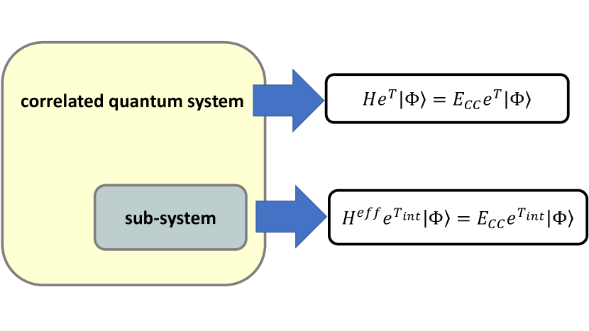
Figure 1: Schematic representation of the SES-CC theorem. The CC energy can be obtained as an effective Hamiltonian eigenvalue.

In Ref.27, we showed that CC approximations have specific classes of SESs. A consequence of the existence of SESs for standard CC approximations is the fact that the corresponding energy can be calculated, in an alternative way to Eq. (6), as an eigenvalue of the active-space non-Hermitian eigenproblem (this fact will be referred to as the SES-CC theorem (see Fig.1))

$$H^{\rm eff}(\mathfrak{h})e^{T_{\rm int}(\mathfrak{h})}|\Phi\rangle=Ee^{T_{\rm int}(\mathfrak{h})}|\Phi\rangle\;.$$ (8)

where

$$H^{\rm eff}(\mathfrak{h})=(P+Q_{\rm int}(\mathfrak{h}))\bar{H}_{\rm ext}(\mathfrak{h})(P+Q_{\rm int}(\mathfrak{h}))\;$$ (9)

and

$$\bar{H}_{\rm ext}(\mathfrak{h})=e^{-T_{\rm ext}(\mathfrak{h})}He^{T_{\rm ext}(\mathfrak{h})}\;.$$ (10)

In Eq.(9), the projection operator $Q_{\rm int}(\mathfrak{h})$ is a projection operator on a sub-space spanned by all Slater determinants generated by $T_{\rm int}(\mathfrak{h})$ acting onto $|\Phi\rangle$. The wave function $|\Psi(\mathfrak{h})\rangle$ defined as

$$|\Psi(\mathfrak{h})\rangle=e^{T_{\rm int}(\mathfrak{h})}|\Phi\rangle\;,$$ (11)

correlates electrons within active space (CAS($\mathfrak{h}$)) while leaving the remaining part of the system uncorrelated. For this reason, we call $|\Psi(\mathfrak{h})\rangle$ a sub-system wave function. These results can be easily extended to the active spaces defined at the spin-orbital level. However, for the closed-shell reference function the use of active spaces defined at the level of spin-orbitals leads to the sub-system wave functions $|\Psi(\mathfrak{h})\rangle$ and corresponding effective Hamiltonian $H^{\rm eff}(\mathfrak{h})$ that break the symmetry of the reference function $|\Phi\rangle$ and total Hamiltonian $H$, respectively (see Fig.2).

Figure 2: Two types of active spaces considered in this paper: (a) orbital definition with the sub-system wave function $|\Psi(\mathfrak{h})\rangle$ preserving the symmetry of the reference function $|\Phi\rangle$ (see Eq.(11), and (b) spin-orbital definition of the active space - in this case the symmetry (especially the spin symmetry) of the sub-system may be broken.

As mentioned earlier, each standard CC approximation is characterized by its own class of SESs (see Ref.27 for details).

The SES-CC theorem is valid for arbitrary SES $\mathfrak{h}$ corresponding to a given CC approximation. For example, for the CCSD approximation, arbitrary non-trivial (i.e., containing at least one active occupied and one virtual active orbitals) SES $\mathfrak{g}^{(N)}(R,S)$ defined at the orbital level, contains either one occupied active orbital or one virtual active orbital. This means that one can form $S_{\rm CCSD}$,

$$S_{\rm CCSD}=n_{o}(2^{n_{v}}-1)+n_{v}(2^{n_{o}}-1)\;,$$ (12)

various SESs and corresponding effective Hamiltonians, that upon diagonalization, reproduce the standard CCSD energy (this formula is a consequence of binomial expansion, and that $k$ active virtual/occupied orbitals can be chosen in ${n_{v}\choose k}$/${n_{o}\choose k}$ different ways). For higher-rank approximations, the number of SESs increases rapidly. In Eq.(12), $n_{o}$ and $n_{v}$ correspond to the number occupied and virtual orbitals. Since in the definition of the effective Hamiltonian, Eqs. (9) and (10), only $T_{\rm ext}(\mathfrak{h})$ is involved, one can view the SES CC formalism with the resulting active-space eigenvalue problem, Eq. (8), as a specific form of a renormalization procedure where external parameters defining the corresponding wave function are integrated out. One should also mention that calculating the CC energy using Eq. (8), is valid for any SES for a given CC approximation defined by cluster operator $T$. In line with the SES-CC theorem, the standard CC energy expression, shown by Eq. (6), can be reproduced when one uses a trivial sub-algebra, which contains no excitations (i.e., active space is spanned by the $|\Phi\rangle$ only).

The SES-CC theorem can be extended to the case when several SES-CC non-Hermitian eigenvalue problems are integrated into the so-called quantum flow (see Refs. 27, 28, 31) composed of coupled low-dimensionality eigenproblems

$$H^{\rm eff}(\mathfrak{h}_{i})e^{T_{\rm int}(\mathfrak{h}_{i})}|\Phi\rangle=Ee^{T_{\rm int}(\mathfrak{h}_{i})}|\Phi\rangle\;(i=1,\ldots,M_{\rm SES})\;,$$ (13)

where $M_{\rm SES}$ is the total number of SESs or active space problems included in the flow. In Ref.28, 31, we demonstrated that problem defined in this way is equivalent (at the solution) to the standard CC equations given by Eqs.(5) and (6) with cluster operator defined as a combination of all unique excitations included in $T_{\rm int}(\mathfrak{h}_{i})$ $(i=1,\ldots,M_{\rm SES})$ operators. This observation allows to (1) capture the local correlation effects in a more controllable way (if all SESs involved in the quantum flow are defined by pairs of active occupied and localized orbitals, then each eigenvalue sub-problem is defined by the effective Hamiltonian, which inherently allows one to define pair density matrix; moreover each ”pair” sub-problem corresponds to a correlation of fours electrons, which using the same density matrix enables one to select subsets of triple and quadruple excitations in additions to singles and doubles), and (2) re-represent the process of solving equations for many-body systems - instead of treating the whole system at once, one can deal with only one reduced-dimension sub-system at the time. In quantum computing, the unitary variant of the SES-CC formalism [28] can also be used to introduce constant-depth quantum algorithms.

It is also interesting to analyze the behavior of the CC equations in the context of the non-interacting sub-subsystem limit (NSL). Let us assume that we partition the entire system $\Delta$ into $K$ sub-systems $\{\Delta_{i}\}_{i=1}^{K}$ and approximate cluster operator contains all components $T_{\Delta_{i}}$ needed to fully correlate individual sub-systems $\Delta_{i}$ in the NSL (for example, for CCSD theory sub-systems $\Delta_{i}$ are two electron systems). Therefore, in the NSL, the cluster operator $T$ and Hamiltonian $H$ can be written (we assume that localized basis set is employed) as sums of components $T_{\Delta_{i}}/H_{\Delta_{i}}$ describing sub-systems:

$$T=\sum_{i=1}^{K}T_{\Delta_{i}}\;\;,\;\;H=\sum_{i=1}^{K}H_{\Delta_{i}}\;,\;$$ (14)

Given the commutativity relations between $H_{\Delta_{i}}$’s ($[H_{\Delta_{i}},H_{\Delta_{j}}]=0$) one can derive the following form of the CC equations in the NSL limit:

$$(P+Q_{\Delta_{m}})[e^{-\sum_{i\neq m}T_{\Delta_{i}}}(\sum_{j=1}^{K}H_{\Delta_{j}})e^{\sum_{k\neq m}T_{\Delta_{k}}}]e^{T_{\Delta_{m}}}|\Phi\rangle=Ee^{T_{\Delta_{m}}}|\Phi\rangle\;,(m=1,\ldots,K)\;,$$ (15)

where $Q_{\Delta_{m}}$ is a projection operator onto excited Slater determinants localized on sub-system $\Delta_{m}$. It takes precisely the same form as equations (13). Henceforth one can view quantum flow equations given by Eqs.(13) as the extension of the properties of the CC equations in the NSL to the interaction regime, where all sub-systems interact. On the other hand, the form of CC equations in NSL is a special case of (8), where groups of active orbitals are at an infinite distance from each other.

III Numerical Simulations

The numerical studies for several benchmark systems, including H4, H6, H8, and Li₂ systems, were performed using occupation-number-representation-based many-body manipulator code (stringMB) that allows one to construct a matrix representation (${\bf A}$) of general second-quantized operators $A$. In particular, stringMB can be used to build matrix representations of the Hamiltonian, the external part of the cluster operator, and exponents of $T_{\rm ext}(\mathfrak{h})$ for arbitrary $\mathfrak{h}$, i.e.,

$$H \rightarrow {\bf H}\;\;,$$ (16)

$$T_{\rm ext}(\mathfrak{h}) \rightarrow {\bf T}_{\rm ext}(\mathfrak{h})\;\;,$$ (17)

$$e^{-T_{\rm ext}(\mathfrak{h})},\;e^{T_{\rm ext}(\mathfrak{h})} \rightarrow e^{-{\bf T}_{\rm ext}(\mathfrak{h})},\;e^{{\bf T}_{\rm ext}(\mathfrak{h})}\;.$$ (18)

Moreover, the stringMB can extract sub-blocks of matrices or their products corresponding to arbitrary sub-space of the entire space. This feature is used to form matrix representations of the effective Hamiltonians $H^{\rm eff}(\mathfrak{h})$.

We chose the STO-3G and 6-31G (for beryllium atom only) basis sets [43, 44] to describe benchmark systems considered here. To provide the numerical illustration of the SES-CC theorem in a variety of situations, for H4 and H6, we chose several geometries corresponding to weakly ($\alpha$=0.500 for H4 and $R_{\rm H-H}=2.0$ a.u. for H6 and H8) and strongly ($\alpha$=0.005 for H4 and $R_{\rm H-H}=3.0$ a.u. for H6) correlated ground states.

IV CC theory and sub-subsystem consistency

In this Section, using the CCSD and CCSDTQ approaches as examples, we will illustrate that solving the CC equation is equivalent to establishing a self-consistency between various sub-systems defined by the corresponding SESs. Specifically, we will illustrate that the diagonalization of effective Hamiltonians corresponding to various SESs reproduces the CC energies obtained with Eq.(6). In Table 1 we collated ground-state eigenvalues $E(\mathfrak{h})$ of various SESs $\mathfrak{h}$ and corresponding effective Hamiltonians $H^{\rm eff}(\mathfrak{h})$ for H4 system in linear ($\alpha=0.500$) and almost square ($\alpha=0.005$) configurations and H6 for $R_{\rm H-H}$=2.0 a.u. and $R_{\rm H-H}$=3.0 a.u. For testing purposes for H4 we used the following CCSD SESs $\mathfrak{h}$: $\mathfrak{g}^{(N)}(1_{R},1_{S})$ with $R=\{2\}$, $S=\{3\}$, $R=\{1\}$, $S=\{3\}$, and $R=\{2\}$, $S=\{4\}$, $\mathfrak{g}^{(N)}(1_{R},2_{S})$ with $R=\{2\}$, $S=\{3,4\}$, and $\mathfrak{g}^{(N)}(2_{R},1_{S})$ with $R=\{1,2\}$, $S=\{3\}$. For each case considered in Table 1, each value of $E(\mathfrak{h})$ reproduces exact value of the CCSD energy $E_{\rm CCSD}$. Analogous situations can be observed for the H6 system with the following SESs: $\mathfrak{g}^{(N)}(1_{R},1_{S})$ with $R=\{3\}$, $S=\{4\}$, $\mathfrak{g}^{(N)}(1_{R},1_{S})$ with $R=\{2\}$, $S=\{4\}$, $\mathfrak{g}^{(N)}(1_{R},1_{S})$ with $R=\{1\}$, $S=\{6\}$, $\mathfrak{g}^{(N)}(1_{R},2_{S})$ with $R=\{1\}$, $S=\{4,5\}$, and $\mathfrak{g}^{(N)}(1_{R},2_{S})$ with $R=\{1\}$, $S=\{4,5\}$ Again, for each case considered in Table 1, each value of $E(\mathfrak{h})$ reproduces exact value of the CCSD energy $E_{\rm CCSD}$.

STO-3G H4 $\alpha$=0.005 $E_{\rm CCSD}$=-1.946325
	$R$=$\{2\}$, $S$=$\{3\}$	$R$=$\{1\}$, $S$=$\{3\}$	$R$=$\{2\}$, $S$=$\{4\}$	$R$=$\{2\}$, $S$=$\{3,4\}$	$R$=$\{1,2\}$, $S$=$\{3\}$
$E_{\mathfrak{h}}$	-1.946325	-1.946325	-1.946325	-1.946325	-1.946325
STO-3G H4 $\alpha=0.500$ $E_{\rm CCSD}$=-2.151004
	$R$=$\{2\}$, $S$=$\{3\}$	$R$=$\{1\}$, $S$=$\{3\}$	$R$=$\{2\}$, $S$=$\{4\}$	$R$=$\{2\}$, $S$=$\{3,4\}$	$R$=$\{1,2\}$, $S$=$\{3\}$
$E_{\mathfrak{h}}$	-2.151004	-2.151004	-2.151004	-2.151004	-2.151004
STO-3G H6 $R_{H-H}=2.0$ a.u. $E_{\rm CCSD}$=-3.217277
	$R$=$\{3\}$, $S$=$\{4\}$	$R$=$\{2\}$, $S$=$\{4\}$	$R$=$\{1\}$, $S$=$\{6\}$	$R$=$\{1\}$, $S$=$\{4,5\}$	$R$=$\{3\}$, $S$=$\{4,5,6\}$
$E_{\mathfrak{h}}$	-3.217277	-3.217277	-3.217277	-3.217277	-3.217277
STO-3G H6 $R_{H-H}=3.0$ a.u. $E_{\rm CCSD}$=-2.967326
	$R$=$\{3\}$, $S$=$\{4\}$	$R$=$\{2\}$, $S$=$\{4\}$	$R$=$\{1\}$, $S$=$\{6\}$	$R$=$\{1\}$, $S$=$\{4,5\}$	$R$=$\{3\}$, $S$=$\{4,5,6\}$
$E_{\mathfrak{h}}$	-2.967326	-2.967326	-2.967326	-2.967326	-2.967326

Table 1: Comparisons of the CCSD energies $E_{\rm CCSD}$ obtained with the standard textbook formula for CC energy with eigenvalues $E_{\mathfrak{h}}$ of effective Hamiltonians acting in SES active spaces defined by various $R$ and $S$ orbital subsets. The tests were performed for H4 system defined by two values of geometry parameter $\alpha$ ($\alpha=0.005$ and $\alpha=0.500$) and H6 system, a linear chain of hydrogen atoms, for $R_{H-H}$=2.0a.u. and $R_{H-H}$=3.0a.u. All energies are reported in Hartree.

In Table 2 we collected $E(\mathfrak{h})$ for spin-orbital definitions of $\mathfrak{h}$ corresponding to the simplest spin-orbital-type active spaces where a single $\alpha$ electron is correlated within one occupied and one virtual active $\alpha$ spin-orbitals. As in the case of the orbital-type SESs, the $E(\mathfrak{h})$’s for H4, H6, and Li₂ reproduce exact values of $E_{\rm CCSD}$.

	H4 ,  $\alpha$=0.005	H6 ,  $R_{\rm H-H}$=2.0a.u.	Li2 ,  $R_{\rm Li-Li}$=2.673Å
	$E_{\rm CCSD}$=-1.946325	$E_{\rm CCSD}$=-3.217277	$E_{\rm CCSD}$=-14.667260
	$R$=$\{1\alpha\}$, $S$=$\{3\alpha\}$	$R$=$\{3\alpha\}$, $S$=$\{5\alpha\}$	$R$=$\{1\alpha\}$, $S$=$\{4\alpha\}$
$E_{\mathfrak{h}}$	-1.946325	-3.217277	-14.667260

Table 2: Comparisons of the CCSD energies $E_{\rm CCSD}$ obtained with the standard textbook formula for CC energy with eigenvalues $E_{\mathfrak{h}}$ of effective Hamiltonians acting in SES active spaces defined by various $R$ and $S$ spin-orbital subsets. For example, $R$=$\{1\alpha\}$, $S$=$\{3\alpha\}$, designates spin-orbital active space spanned by $\alpha$ spin associated with orbital $1$ and $\alpha$ spin associated with orbital $3$. The $R_{\rm Li-Li}=2.673\AA$ corresponds to near equilibrium geometry of the Li₂ molecule. All energies are reported in Hartree.

As a part of the discussion regarding the possibility of breaking symmetries of the whole quantum system, it is interesting to explore the possibility of breaking orbital energy degeneracies of the sub-system. To extend the previous paragraph’s discussion, we chose the Be atom in the 6-31 basis set as a benchmark system. The degenerate RHF orbitals 3,4 and 5, as well as 7, 8, and 9, correspond to different $p$ shells. In our simulations, we used the following active spaces: (1) $R$=$\{2\}$, $S$=$\{3\}$, (2) $R$=$\{2\}$, $S$=$\{3,4\}$, (3) $R$=$\{2\}$, $S$=$\{3,4,5\}$, and (4) $R$=$\{2\}$, $S$=$\{3,9\}$. While the active space (3) would usually be involved in typical quantum chemical calculations, the active spaces (1), (2), and (4) correspond to the unusual situation where the degeneracies of the orbital energies are broken. The active space (4) also contains two active virtual orbitals corresponding to two separate $p$ shells. Despite this fact, as seen from Table 3, the SES-CC theorem produces energies equal to the CCSD energy in all situations. This is yet another illustration of an interesting feature of the SES-CC theorem associated with various scenarios for symmetry breaking.

	Be atom
	$E_{\rm CCSD}$=-14.613518
	$R$=$\{2\}$, $S$=$\{3\}$	$R$=$\{2\}$, $S$=$\{3,4\}$	$R$=$\{2\}$, $S$=$\{3,4,5\}$	$R$=$\{2\}$, $S$=$\{3,9\}$
$E_{\mathfrak{h}}$	-14.613518	-14.613518	-14.613518	-14.613518

Table 3: Comparisons of the CCSD energies $E_{\rm CCSD}$ obtained with the standard textbook formula for CC energy with eigenvalues $E_{\mathfrak{h}}$ of effective Hamiltonians acting in the SES generated active spaces defined by various $R$ and $S$ orbital subsets for the Be atom in the 6-31G basis set. All energies are reported in Hartree.

	H6 ,  $R_{\rm H-H}$=2.0a.u.
	$E_{\rm CCSDTQ}$=-3.217699
	$R$=$\{2,3\}$, $S$=$\{4,5\}$	$R$=$\{1,2\}$, $S$=$\{5,6\}$	$R$=$\{3\}$, $S$=$\{4\}$	$R$=$\{3\}$, $S$=$\{4,5\}$
$E_{\mathfrak{h}}$	-3.217699	-3.217699	-3.217699	-3.217699

Table 4: Comparisons of the CCSDTQ energies $E_{\rm CCSDTQ}$ obtained with the standard textbook formula for CC energy with eigenvalues $E_{\mathfrak{h}}$ of effective Hamiltonians acting in the SES generated active spaces defined by various $R$ and $S$ orbital subsets for the H6 linear chain with $R_{H-H}=2.0$ a.u. in the STO-3G basis set. All energies are reported in Hartree.

	H8 ,  $R_{\rm H-H}$=2.0a.u.
	$E_{\rm CCSDTQ}$=-4.286013
	$R$=$\{3,4\}$, $S$=$\{5,6\}$	$R$=$\{1,2\}$, $S$=$\{7,8\}$	$R$=$\{4\}$, $S$=$\{5\}$	$R$=$\{4\}$, $S$=$\{5,6\}$
$E_{\mathfrak{h}}$	-4.286013	-4.286013	-4.286013	-4.286013

Table 5: Comparisons of the CCSDTQ energies $E_{\rm CCSDTQ}$ obtained with the standard textbook formula for CC energy with eigenvalues $E_{\mathfrak{h}}$ of effective Hamiltonians acting in the SES generated active spaces defined by various $R$ and $S$ orbital subsets for the H8 linear chain with $R_{H-H}=2.0$ a.u. in the STO-3G basis set. All energies are reported in Hartree.

As mentioned earlier, the SES-CC theorem is valid for standard CC approximation defined by a given excitation level. While our discussion has focused so far on the CCSD methods, in the following part of this Section, we will discuss the SES-CC theorem in the context of the CCSDTQ formulation. To this end, we performed a series of calculations for systems containing more than four correlated electrons where the CCSDTQ approach does not correspond to the exact theory. In Tables 4 and 5, we collated the results of the SES-CC simulations for H6 and H8 models in the STO-3G basis set.

For H6, we considered two types of SES-CC active spaces containing two occupied and two virtual orbitals, i.e., $R$=$\{2,3\}$, $S$=$\{4,5\}$ and $R$=$\{1,2\}$, $S$=$\{5,6\}$. While the first active space is directly related to the corresponding ground-state problem, the second one contains excited Slater determinants (with respect to the reference function $|\Phi\rangle$) that represent a small contribution to the ground-state wave function. In both cases, the diagonalization of the corresponding effective Hamiltonians $H^{\rm eff}(\mathfrak{h})$ leads to the eigenvalues $E_{\mathfrak{h}}$ exactly reproducing the CCSDTQ energy $E_{\rm CCSDTQ}$. One should stress that the above active spaces are SES-CC spaces for the CCSDTQ level of the theory (the CCSDTQ ansatz based on the $T_{\rm int}(\mathfrak{h})$ operator generates FCI-type expansion in these active spaces) and not for the CCSD level of theory. However, as discussed in Ref.27, the SESs for higher-level theory contain all SESs for lower-rank approaches. To provide numerical confirmation of this statement, we performed calculations using CCSD-type SES, i.e., $R$=$\{3\}$, $S$=$\{4\}$ and $R$=$\{3\}$, $S$=$\{4,5\}$. Again, in both cases we were able to reproduce the CCSDTQ energies.

Analogous analysis can be performed for the H8 system (see Table 5). For all types of SES active spaces discussed in Table 5, we reproduced the exact values of the CCSDTQ energy.

For H6 and H8 systems, using the CCSDTQ formalism, we also performed simulations based on the spin-orbital definition of $\mathfrak{h}$, e.g., $R$=$\{2\alpha\}$, $S$=$\{4\alpha\}$ (H6) and $R$=$\{4\alpha\}$, $S$=$\{6\alpha\}$ (H8) that reproduce the exact values of the CCSDTQ energies using sub-systems composed of a single correlated electron in two active spin-orbitals.

V Conclusions

Our numerical tests indicate that CC energies can be obtained alternatively to the textbook energy formula by diagonalizing effective Hamiltonians for sub-systems defined in appropriate active spaces. In the present studies, we focused on the closed-shell CC formulations where the active spaces can be determined in terms of active orbitals or active spin-orbitals. We demonstrated that the CC energies for the CCSD and CCSDTQ approaches could be exactly reproduced by using these two types of active spaces. In the extreme case, we showed that the CC energy could be reproduced by a sub-system (in the sense of sub-system wave function defined by Eq.(11)) composed of one active electron in two active $\alpha$-type spin-orbitals. We also demonstrated that the alternative ways of obtaining CC energy could be viewed as an analog to the asymptotic behavior of the CC formalism in the non-interacting sub-system limit in the presence of interactions. These facts have interesting consequences regarding how CC theory should be interpreted and how a new class of CC approximations can be formulated. The main conclusions are listed below:

• From the SES-CC perspective, the standard single-reference CC Ansatz can be viewed as a renormalization procedure where energies describing all possible SES-CC sub-systems are calculated self-consistently.

• The quantum flow formalism introduced and discussed in Refs.27, 28 exploits this feature to define a new class of approximations that self-consistently correlate pre-defined classes of sub-systems. At the convergence, all ground-state eigenvalues of all effective Hamiltonians are equal and correspond to the approximate ground-state energy of the entire system.

• The size-consistency of approximations designed based on quantum flow equations is guaranteed by the so-called equivalence theorem (see Refs.28, 31)

• The quantum flow approach provides a natural way to capture the quantum system’s sparsity. This is because each sub-system is described in terms of the corresponding non-Hermitian (Hermitian, for unitary CC flows) eigenvalue problems defined by Hamiltonian $H^{\rm eff}(\mathfrak{h}_{i})$ (see Eq.(13)), which enables one in a natural way to determine sub-system’s one-body density matrix and select sub-system’s natural orbitals to select class of the most important cluster amplitudes as in the local CC formulations [45, 46, 17, 47]).

• The quantum flow equations represent a quantum many-body problem in terms of coupled, reduced-dimensionality, and computable (both from the classical and quantum computing perspective) sub-problems. It can provide a new way of looking at the orthogonality catastrophe discussed in Ref.[48] (see also Refs. 49, 50, 51, 48) both in the context of classical and quantum computing.

A part of the ongoing development is associated with the formulation of excited-state extensions of quantum flows that guarantee the size intensity of the quantum flows. The process assures this feature by picking up excited states localized on a chosen sub-system. This is especially important for unitary CC flows discussed in Ref.28, and excited-state applications of downfolding techniques in quantum computing.[52].

VI Acknowledgement

This work was supported by the “Embedding Quantum Computing into Many-body Frameworks for Strongly Correlated Molecular and Materials Systems” project, which is funded by the U.S. Department of Energy(DOE), Office of Science, Office of Basic Energy Sciences, the Division of Chemical Sciences, Geosciences, and Biosciences. All simulations were performed using Pacific Northwest National Laboratory (PNNL) computational resources. PNNL is operated for the U.S. Department of Energy by the Battelle Memorial Institute under Contract DE-AC06-76RLO-1830.

AUTHOR DECLARATIONS

Conflict of Interest

The author has no conflicts of interest to declare.

DATA AVAILABILITY

The data that support the findings of this study are available from the corresponding authors upon reasonable request.

References

- Coester [1958] F. Coester, “Bound states of a many-particle system,” Nucl. Phys. 7, 421–424 (1958).
- Coester and Kümmel [1960] F. Coester and H. Kümmel, “Short-range correlations in nuclear wave functions,” Nucl. Phys. 17, 477–485 (1960).
- Čížek [1966] J. Čížek, “On the correlation problem in atomic and molecular systems. calculation of wavefunction components in ursell-type expansion using quantum-field theoretical methods,” J. Chem. Phys. 45, 4256–4266 (1966).
- Paldus, Čížek, and Shavitt [1972] J. Paldus, J. Čížek, and I. Shavitt, “Correlation problems in atomic and molecular systems. iv. extended coupled-pair many-electron theory and its application to the b molecule,” Phys. Rev. A 5, 50–67 (1972).
- Purvis and Bartlett [1982] G. Purvis and R. Bartlett, “A full coupled-cluster singles and doubles model: The inclusion of disconnected triples,” J. Chem. Phys. 76, 1910–1918 (1982).
- Arponen [1983] J. Arponen, “Variational principles and linked-cluster exp s expansions for static and dynamic many-body problems,” Ann. Phys. 151, 311–382 (1983).
- Bishop and Kümmel [1987] R. F. Bishop and H. Kümmel, “The coupled-cluster method,” Phys. Today 40, 52 (1987).
- Paldus and Li [1999] J. Paldus and X. Li, “A critical assessment of coupled cluster method in quantum chemistry,” Adv. Chem. Phys. 110, 1–175 (1999).
- Crawford and Schaefer [2000] T. D. Crawford and H. F. Schaefer, “An introduction to coupled cluster theory for computational chemists,” Reviews in computational chemistry 14, 33–136 (2000).
- Bartlett and Musiał [2007] R. J. Bartlett and M. Musiał, “Coupled-cluster theory in quantum chemistry,” Rev. Mod. Phys. 79, 291–352 (2007).
- Scheiner et al. [1987] A. C. Scheiner, G. E. Scuseria, J. E. Rice, T. J. Lee, and H. F. Schaefer III, “Analytic evaluation of energy gradients for the single and double excitation coupled cluster (ccsd) wave function: Theory and application,” The Journal of chemical physics 87, 5361–5373 (1987).
- Sinnokrot, Valeev, and Sherrill [2002] M. O. Sinnokrot, E. F. Valeev, and C. D. Sherrill, “Estimates of the ab initio limit for - interactions: The benzene dimer,” Journal of the American Chemical Society 124, 10887–10893 (2002).
- Slipchenko and Krylov [2002] L. V. Slipchenko and A. I. Krylov, “Singlet-triplet gaps in diradicals by the spin-flip approach: A benchmark study,” The Journal of chemical physics 117, 4694–4708 (2002).
- Tajti et al. [2004] A. Tajti, P. G. Szalay, A. G. Császár, M. Kállay, J. Gauss, E. F. Valeev, B. A. Flowers, J. Vázquez, and J. F. Stanton, “Heat: High accuracy extrapolated ab initio thermochemistry,” The Journal of chemical physics 121, 11599–11613 (2004).
- Crawford [2006] T. D. Crawford, “Ab initio calculation of molecular chiroptical properties,” Theoretical Chemistry Accounts 115, 227–245 (2006).
- Parkhill, Lawler, and Head-Gordon [2009] J. A. Parkhill, K. Lawler, and M. Head-Gordon, “The perfect quadruples model for electron correlation in a valence active space,” The Journal of chemical physics 130, 084101 (2009).
- Riplinger and Neese [2013] C. Riplinger and F. Neese, “An efficient and near linear scaling pair natural orbital based local coupled cluster method,” The Journal of chemical physics 138, 034106 (2013).
- Yuwono, Magoulas, and Piecuch [2020] S. H. Yuwono, I. Magoulas, and P. Piecuch, “Quantum computation solves a half-century-old enigma: Elusive vibrational states of magnesium dimer found,” Science Advances 6, eaay4058 (2020).
- Stoll [1992] H. Stoll, “Correlation energy of diamond,” Physical Review B 46, 6700 (1992).
- Hirata et al. [2004] S. Hirata, R. Podeszwa, M. Tobita, and R. J. Bartlett, “Coupled-cluster singles and doubles for extended systems,” J. Chem. Phys. 120, 2581–2592 (2004).
- Katagiri [2005] H. Katagiri, “Equation-of-motion coupled-cluster study on exciton states of polyethylene with periodic boundary condition,” The Journal of chemical physics 122, 224901 (2005).
- Booth et al. [2013] G. H. Booth, A. Grüneis, G. Kresse, and A. Alavi, “Towards an exact description of electronic wavefunctions in real solids,” Nature 493, 365 (2013).
- Degroote et al. [2016] M. Degroote, T. M. Henderson, J. Zhao, J. Dukelsky, and G. E. Scuseria, “Polynomial similarity transformation theory: A smooth interpolation between coupled cluster doubles and projected bcs applied to the reduced bcs hamiltonian,” Physical Review B 93, 125124 (2016).
- McClain et al. [2017] J. McClain, Q. Sun, G. K.-L. Chan, and T. C. Berkelbach, “Gaussian-based coupled-cluster theory for the ground-state and band structure of solids,” Journal of chemical theory and computation 13, 1209–1218 (2017).
- Wang and Berkelbach [2020] X. Wang and T. C. Berkelbach, “Excitons in solids from periodic equation-of-motion coupled-cluster theory,” Journal of Chemical Theory and Computation 16, 3095–3103 (2020).
- Haugland et al. [2020] T. S. Haugland, E. Ronca, E. F. Kjønstad, A. Rubio, and H. Koch, “Coupled cluster theory for molecular polaritons: Changing ground and excited states,” Phys. Rev. X 10, 041043 (2020).
- Kowalski [2018] K. Kowalski, “Properties of coupled-cluster equations originating in excitation sub-algebras,” J. Chem. Phys. 148, 094104 (2018).
- Kowalski [2021] K. Kowalski, “Dimensionality reduction of the many-body problem using coupled-cluster subsystem flow equations: Classical and quantum computing perspective,” Physical Review A 104, 032804 (2021).
- Bauman et al. [2019] N. P. Bauman, E. J. Bylaska, S. Krishnamoorthy, G. H. Low, N. Wiebe, C. E. Granade, M. Roetteler, M. Troyer, and K. Kowalski, “Downfolding of many-body hamiltonians using active-space models: Extension of the sub-system embedding sub-algebras approach to unitary coupled cluster formalisms,” J. Chem. Phys. 151, 014107 (2019).
- Metcalf et al. [2020] M. Metcalf, N. P. Bauman, K. Kowalski, and W. A. de Jong, “Resource-efficient chemistry on quantum computers with the variational quantum eigensolver and the double unitary coupled-cluster approach,” Journal of Chemical Theory and Computation 16, 6165–6175 (2020), pMID: 32915568, https://doi.org/10.1021/acs.jctc.0c00421 .
- Bauman and Kowalski [2022] N. P. Bauman and K. Kowalski, “Coupled cluster downfolding theory: towards universal many-body algorithms for dimensionality reduction of composite quantum systems in chemistry and materials science,” Materials Theory 6, 1–19 (2022).
- Kowalski and Bauman [2020] K. Kowalski and N. P. Bauman, “Sub-system quantum dynamics using coupled cluster downfolding techniques,” The Journal of Chemical Physics 152, 244127 (2020), https://doi.org/10.1063/5.0008436 .
- Jankowski and Kowalski [1996] K. Jankowski and K. Kowalski, “Approximate coupled cluster methods based on a split-amplitude strategy,” Chemical physics letters 256, 141–148 (1996).
- Nooijen [1999] M. Nooijen, “Combining coupled cluster and perturbation theory,” The Journal of Chemical Physics 111, 10815–10826 (1999).
- He, Li, and Evangelista [2022] N. He, C. Li, and F. A. Evangelista, “Second-order active-space embedding theory,” Journal of Chemical Theory and Computation 18, 1527–1541 (2022).
- Callahan, Lange, and Berkelbach [2021] J. M. Callahan, M. F. Lange, and T. C. Berkelbach, “Dynamical correlation energy of metals in large basis sets from downfolding and composite approaches,” The Journal of Chemical Physics 154, 211105 (2021).
- Kvaal [2022] S. Kvaal, “Three lagrangians for the complete-active space coupled-cluster method,” arXiv preprint arXiv:2205.08792 (2022).
- Noga and Bartlett [1987] J. Noga and R. J. Bartlett, “The full ccsdt model for molecular electronic structure,” J. Chem. Phys. 86, 7041–7050 (1987).
- Noga and Bartlett [1988] J. Noga and R. J. Bartlett, “Erratum: The full ccsdt model for molecular electronic structure [j. chem. phys. 86, 7041 (1987)],” J. Chem. Phys. 89, 3401–3401 (1988).
- Scuseria and Schaefer [1988] G. E. Scuseria and H. F. Schaefer, “A new implementation of the full ccsdt model for molecular electronic structure,” Chem. Phys. Lett. 152, 382–386 (1988).
- Oliphant and Adamowicz [1991] N. Oliphant and L. Adamowicz, “Coupled-cluster method truncated at quadruples,” J. Chem. Phys. 95, 6645–6651 (1991).
- Kucharski and Bartlett [1991] S. A. Kucharski and R. J. Bartlett, “Recursive intermediate factorization and complete computational linearization of the coupled-cluster single, double, triple, and quadruple excitation equations,” Theor. Chem. Acc. 80, 387–405 (1991).
- Hehre, Stewart, and Pople [1969] W. J. Hehre, R. F. Stewart, and J. A. Pople, “self-consistent molecular-orbital methods. i. use of gaussian expansions of slater-type atomic orbitals,” The Journal of Chemical Physics 51, 2657–2664 (1969).
- Hehre, Ditchfield, and Pople [1972] W. J. Hehre, R. Ditchfield, and J. A. Pople, “Self-consistent molecular orbital methods. xii. further extensions of gaussian-type basis sets for use in molecular orbital studies of organic molecules,” J. Chem. Phys. 56, 2257–2261 (1972).
- Neese, Wennmohs, and Hansen [2009] F. Neese, F. Wennmohs, and A. Hansen, “Efficient and accurate local approximations to coupled-electron pair approaches: An attempt to revive the pair natural orbital method,” The Journal of chemical physics 130, 114108 (2009).
- Neese, Hansen, and Liakos [2009] F. Neese, A. Hansen, and D. G. Liakos, “Efficient and accurate approximations to the local coupled cluster singles doubles method using a truncated pair natural orbital basis,” The Journal of chemical physics 131, 064103 (2009).
- Riplinger et al. [2016] C. Riplinger, P. Pinski, U. Becker, E. F. Valeev, and F. Neese, “Sparse maps- a systematic infrastructure for reduced-scaling electronic structure methods. ii. linear scaling domain based pair natural orbital coupled cluster theory,” J. Chem. Phys. 144, 024109 (2016).
- Lee et al. [2022] S. Lee, J. Lee, H. Zhai, Y. Tong, A. M. Dalzell, A. Kumar, P. Helms, J. Gray, Z.-H. Cui, W. Liu, et al., “Is there evidence for exponential quantum advantage in quantum chemistry?” arXiv preprint arXiv:2208.02199 (2022).
- Kohn [1999] W. Kohn, “Nobel lecture: Electronic structure of matter—wave functions and density functionals,” Reviews of Modern Physics 71, 1253 (1999).
- Chan [2012] G. K.-L. Chan, “Low entanglement wavefunctions,” Wiley Interdisciplinary Reviews: Computational Molecular Science 2, 907–920 (2012).
- McClean et al. [2014] J. R. McClean, R. Babbush, P. J. Love, and A. Aspuru-Guzik, “Exploiting locality in quantum computation for quantum chemistry,” The journal of physical chemistry letters 5, 4368–4380 (2014).
- Bauman, Low, and Kowalski [2019] N. P. Bauman, G. H. Low, and K. Kowalski, “Quantum simulations of excited states with active-space downfolded hamiltonians,” The Journal of Chemical Physics 151, 234114 (2019).