The Space of Adversarial Strategies

Abstract

Adversarial examples, inputs designed to induce worst-case behavior in machine learning models, have been extensively studied over the past decade. Yet, our understanding of this phenomenon stems from a rather fragmented pool of knowledge; at present, there are a handful of attacks, each with disparate assumptions in threat models and incomparable definitions of optimality. In this paper, we propose a systematic approach to characterize worst-case (i.e., optimal) adversaries. We first introduce an extensible decomposition of attacks in adversarial machine learning by atomizing attack components into surfaces and travelers. With our decomposition, we enumerate over components to create $576$ attacks ($568$ of which were previously unexplored). Next, we propose the Pareto Ensemble Attack (PEA): a theoretical attack that upper-bounds attack performance. With our new attacks, we measure performance relative to the PEA on: both robust and non-robust models, seven datasets, and three extended $\ell_{p}$-based threat models incorporating compute costs, formalizing the Space of Adversarial Strategies. From our evaluation we find that attack performance to be highly contextual: the domain, model robustness, and threat model can have a profound influence on attack efficacy. Our investigation suggests that future studies measuring the security of machine learning should: (1) be contextualized to the domain & threat models, and (2) go beyond the handful of known attacks used today.

1 Introduction

It is well-known that machine learning models are vulnerable to adversarial examples—inputs designed to induce worst-case behavior. Seminal papers have introduced a suite of varying techniques for producing adversarial examples, each with their own unique threat models, strengths, and weaknesses [22, 39, 7, 35, 33]. Every generation of research yields the next evolution of attacks, designed to overcome prior defenses. It is unclear whether this evolution will ever converge, yet it is apparent that there are some attacks that have “survived” modern defenses. Specifically, the accepted baselines for evaluating defenses are converging to a small set of largely fixed attacks and threat models.

This observation on the fixed nature of commonly used attacks speaks to a broader and more fundamental problem in the way we evaluate the trustworthiness of machine learning systems: our understanding of adversaries has been derived from a union of works with disjoint assumptions and underlying threat models. As a consequence, it is challenging to draw any universal truths from a rather fragmented (and broadly incomparable) pool of knowledge. Subsequently, comparisons between attacks and attempts at characterizing the worst-case adversary have been through the lens of a specific threat model and defined with respect to a small handful of attacks, making it difficult to discern the true strength of claims on what is good (or even best) and when.

In this paper, we introduce a systematic approach to determine worst-case adversaries. We first introduce $568$ new attacks by anatomizing seminal attacks into interchangeable components, therein enabling a meaningful evaluation of model robustness against an expansive attack space. With this decomposition, we formalize an extensible Space of Adversarial Strategies: the set of attacks considered by an adversary under a specific threat model and domain. We then empirically approximate the Pareto Ensemble Attack (PEA): a theoretical attack which upper-bounds attack performance by returning the optimal set of adversarial examples for a given threat model and dataset. We then use the PEA to explore a fundamental question: Does an optimal attack exist?

Our analysis begins by decomposing seminal attacks in adversarial machine learning. We observe that all known attacks are broadly built from two components: (1) a surface, and (2) a traveler. Surfaces encode the traversable attack space (often as the gradient of a cost function), while travelers are “vehicles” that navigate a surface to meet adversarial goals. Attack components live within surfaces and travelers, which characterize attack behavior, such as building crude surfaces that favor meeting adversarial goals without regard to budget, or vice-versa. Our decomposition allows us to (a) generalize attacks in an extensible manner, and (b) naturally construct new (and known) attacks by permuting attack components.

From our decomposition, we permute attack components to build a previously unexplored attack space, yielding $568$ new attacks. We then measure attack performance through the PEA, which is built by forming the lower envelope of measured model accuracy across attacks over the budget consumed. In other words, the PEA bounds the performance an individual attack could achieve. We rank attacks with respect to the PEA by measuring the difference in areas of their performance curves. Our approach not only gives us a comparable definition of optimality, but also a mechanism by which we can measure the merit of individual attacks.

Our evaluation across seven datasets, three threat models, and robust (through adversarial training) versus non-robust models found relative attack performance to be highly contextual. Specifically, (1) the domain and threat model can have a profound effect (especially if the trained model is robust), and (2) even the advantage of certain component choices is sensitive to these factors, as well as other paired components.

We make the following contributions:

• We propose a decomposition of attacks in adversarial machine learning by atomizing attack components into two main layers, surfaces and travelers. Our decomposition readily enables extensions of new components.

• We characterize the attack space by permuting components of known attacks, yielding $568$ new attacks.

• We introduce a systematic approach to compare the efficacy of attacks. We first build the Pareto Ensemble Attack from the performance curves of attacks and rank their relative performance.

• We instantiate and enumerate over a hypothesis space to identify which strategies perform better than others under a given threat model.

2 Background

2.1 Threat Models

Adversaries have historically had one of two goals: minimizing model accuracy [39, 35, 32, 53] or maximizing model loss [22, 33, 3]. The risks associated with minimizing model accuracy are often exemplified by vehicles misclassifying traffic signs [19], intrusion detection systems permitting malicious entities entry [59], medical misdiagnoses [20], among other failures. Maximizing model loss serves two purposes: (1) it is a surrogate for minimizing model accuracy (as, the inverse is performed to maximize model accuracy during model training), and (2) it aids in transferability attacks [37, 55, 38, 18]. In this work, we focus on minimizing model accuracy and defer the explorations of transferability to future work.

In the context of minimizing model accuracy, translating the risks above into an optimization objective to be solved by an adversary is commonly written as: |l| ϵ∥ϵ∥_p f (x + ϵ) ≠ ^y x + ϵ∈B_ϕ(x).

where we are given a victim model $f$, a sample $x$, label $\hat{y}$, a self-imposed budget $\phi$ measured under some $\ell_{p}$-norm. Conceptually, the adversary searches within some self-imposed norm-ball $\mathcal{B}$ of radius $\phi$, centered at $x$ for a “small” change $\epsilon$ that, when applied to $x$, yields the desired goal.

With adversarial goals and capabilities defined, the final component of threat models pertains to access. Specifically, subsequent works have shown that adversaries need not have direct access to the victim model $f$ to produce adversarial examples; models trained on similar data have similar decision manifolds, and thus, adversarial examples can “transfer” from one model to another [37, 55, 38]. When access is restricted (and thus, transferability is exploited), such threat models are called “grey-” or “black-box”, while full access to the victim model is called a “white-box” threat model. In this paper, we focus on white-box threat models as they represent the worst-case adversaries (in that they can produce adversarial examples with the tightest $\ell_{p}$-norm constraints). However, our decomposition and performance measurements can be directly applied to grey- and black-box threat models as well, which we further discuss in section 6.

On $\ell_{p}$-norms. As shown in subsection 2.1, the “cost” for crafting adversarial examples has been predominantly measured through $\ell_{p}$-norms. Informally, adversarial examples induce a misclassification between human and machine; $\ell_{p}$-bounded examples attempt to meet this definition. This concept arose from attacks on images, in that attacks would produce adversarial examples whose perturbations were invisible to humans, yet influential on models. $\ell_{p}$-norms are becoming an increasingly controversial topic, in that it has been debated if they have meaningful interpretations in non-visual domains [48], or even visual domains [10], or if they are useful at all [47]. Regardless, attacks have broadly converged on optimizing under $\ell_{0}$, $\ell_{2}$, or $\ell_{\infty}$, and thus we focus our study on those.

2.2 Attack Algorithms

Here we briefly discuss the attack algorithms used in our decomposition (specifically, the unique components they introduce). We study these algorithms specifically due to their prevalence across works in adversarial machine learning [42].

Basic Iterative Method (BIM). BIM [29] is an iterative extension of Fast Gradient Sign Method (FGSM) [22]. BIM is an $\ell_{\infty}$-based attack that perturbs based on the gradient of a cost function, typically Cross-Entropy (CE). It often uses Stochastic Gradient Descent (SGD) as its optimizer for finding adversarial examples.

Projected Gradient Descent (PGD). PGD [33] is widely regarded as the state-of-the-art in crafting algorithms. PGD is identical to BIM, with the exception of a Random-Restart preprocessing step, wherein inputs are initially randomly perturbed within an $\ell_{\infty}$ ball.

Jacobian-based Saliency Map Approach (JSMA). The JSMA [39] is an $\ell_{0}$-based attack that is unique in its definition of a saliency map; a heuristic applied to the model Jacobian to determine the most salient feature to perturb in a given iteration. Unlike most other attacks, it does not rely on a cost function, but rather uses the model Jacobian directly. In our decomposition, we denote the JSMA saliency map as SM_J. The JSMA uses SGD as its optimizer.

DeepFool (DF). DF [35] is an $\ell_{2}$-based attack which models crafting adversarial examples as a projection onto the decision boundary. We find that we can model this projection as a saliency map, much like the JSMA, which we denote as SM_D. Similar to the JSMA, DF relies on the model Jacobian, does not have a cost function, and uses SGD.

Carlini-Wagner Attack (CW). CW [7] is an $\ell_{2}$-based attack that is unique across several dimensions: (1) it uses a custom loss, which we label Carlini-Wagner Loss (CWL), (2) introduces the Change of Variables technique, which ensures that, during crafting, the intermediate adversarial examples always comply with a set of box constraints, and (3) uses Adam as its optimizer for finding adversarial examples.

AutoAttack (AA). AA [15] is an ensemble attack consisting of three different white-box attacks (as well as one black-box attack). This ensemble is unique in that all of its attacks are parameter free (except for the number of iterations to run attacks for). Its white-box attacks are: (1) Auto Projected Gradient Descent - Cross Entropy (APGD-CE), which is PGD with the Momentum Best Start optimizer, (2) Auto Projected Gradient Descent - Difference of Logits Ratio (APGD-DLR), which is APGD-CE but with Difference of Logits Ratio Loss, and (3) Fast Adaptive Boundary Attack [13] (FAB), which is similar to DeepFool, but it’s optimizer Backward Stochastic Gradient Descent applies a biased gradient step and a backward step to stay close to the original point.

3 Decomposing AML

From analysis of popular attacks (discussed in subsection 2.2), we find that attacks broadly perform two main functions to produce adversarial examples, they: (1) manipulate $x$, such as with Random-Restart, or (2) manipulate gradients, such as by using a saliency map. We use this observation as a starting point for our decomposition; components that do the former are part of the traveler and ones that do the latter are within the surface. Through this generalization, an attack can be seen as, simply, a choice of values for each of these components rather than a unique, incomparable entity.

Importantly, these components are broadly mutually compatible with one another, in that one could omit, add, or swap them when building an attack. We exploit this property when permuting components, therein yielding a vast space of attacks, some of which are known, but most of which are not. This modular view of attacks not only allows us to build this vast space, but also makes the framework highly extensible by nature; new attacks can add on new choices for components or even new components entirely. A summary of the evaluated components in this paper and the compositions of well-known attacks are shown in Table 1.

For the remainder of this section, we describe: (1) the components that constitute a surface and their options, (2) the layers that define a traveler and associated configurations, and (3) a characterization of the attack space. An overview of the composition of the surface and traveler, and their interaction is shown in Figure 1. All symbols defined in this section (and in the remainder of the paper) can be found in appendix D.

Attack Algorithms
Surface Components		Traveler Components
Losses:	Cross-Entropy Carlini-Wagner Loss Identity Loss Difference of Logits Ratio Loss	Random-Restart:	Enabled, Disabled
Saliency Maps:	SMJ, SMD, SMI	Change of Variables:	Enabled, Disabled
$\ell_{p}$-norm	$\ell_{0}$, $\ell_{2}$, $\ell_{\infty}$	Optimizer:	SGD, Adam, MBS, BWSGD

BIM PGD JSMA DF CW APGD-CE APGD-DLR FAB CE CWL IL DLR SM_J SM_D SM_I $\ell_{0}$ $\ell_{2}$ $\ell_{\infty}$ RR CoV SGD Adam MBS BWSGD

Table 1: Attack Component Decomposition.

Figure 1: Flow of composition between the surface and traveler to construct an attack. Required components have bold outlines while optional components have dotted outlines.

3.1 Surfaces

Surfaces, which encode the traversable attack space, are built from: (1) the model Jacobian, (2) the gradient of a loss function, (3) the application of a saliency map, and (4) an $\ell_{p}$-norm. context of crafting adversarial examples.

Model Jacobian. At the heart of every surface (and thus, every attack) is the model Jacobian. The Jacobian $\mathbf{J}{}$ of a model with respect to a sample $x$ encodes the influence each feature $i$ in $x$ has over each class. While most attack papers encode perturbations as a function of the gradient of a loss function, such computations necessarily involve computing a portion (at least) of the model Jacobian (whether attacks require the full model Jacobian is a matter of design choice). This is evident via application of the chain rule:

$$\frac{\partial L(f(x),\hat{y})}{\partial x}=\frac{\partial L(f(x),\hat{y})}{\partial f(x)}\cdot\frac{\partial f(x)}{\partial x}=\frac{\partial L(f(x),\hat{y})}{\partial f(x)}\cdot\textbf{J}$$

Importantly, computing a Jacobian is computationally expensive, on the order of $\mathcal{O}{}(d\cdot c)$, where $d$ describes the dimensionality of $x$ (i.e., the number of features) and $c$ describes the number of classes. Thus, attacks that require the full model Jacobian (e.g., JSMA and DF) must pay a (sometimes substantial) cost in compute resources to produce adversarial examples—a fact largely overlooked. This component is perhaps the one with the greatest potential for extensibility. For instance, black-box attacks or those wanting to overcome obfuscated gradients [2] could opt to use Backwards Pass Differentiable Approximation (BPDA) [2] to obtain a jacobian rather than a traditional backwards pass.

Loss Functions. Perhaps the most popular design choice in attack algorithms is to perturb features based on the gradient of a loss function. The intuition is straightforward: we rely on surrogate measurements to learn parameters that have maximal accuracy during training, and thus, we can exploit these same measures to produce samples that induce minimal accuracy. This is commonly Cross-Entropy (CE) loss:

$$\sum_{i}^{c}-\hat{y}_{i}\cdot\log(y_{i})$$

where $c$ is the number of classes, $\hat{y}_{i}$ is the label as a one-hot encoded vector, and $y_{i}$ is the output of the softmax function.

Aside from CE loss, other attack philosophies instead opt for custom loss functions that explicitly encode adversarial objectives, such as Carlini-Wagner Loss (CWL):

$$\lVert\delta\rVert^{p}_{p}+c\cdot\max(f_{\hat{y}}(x)-\max\{f_{i}(x):i\neq\hat{y}\},0)$$

where $p$ is the target $\ell_{p}$-norm to optimize under and $c$ is a hyperparameter that controls the trade-off between the distortion introduced and misclassification.

Similar to the latter half of CWL, the Difference of Logits Ratio Loss (DLR) takes the difference between the true logit and the largest non-true-class logit. However, this loss function also divides by the difference between the largest logit ($f_{\pi_{1}}(x)$) and the third largest logit ($f_{\pi_{3}}(x)$), as follows:

$$-\frac{f_{\hat{y}}(x)-\max\{f_{i}(x):i\neq\hat{y}\}}{f_{\pi_{1}}(x)-f_{\pi_{3}}(x)}$$

Finally, some attacks do not have an explicit loss function (such as JSMA or DF) and instead rely on information at other layers in the surface to produce adversarial examples (e.g., through saliency maps). To support this generalization, we implement a pseudo-identity loss function, Identity Loss (IL), which simply returns the $\hat{y}$th model logit component.

Saliency Maps. Saliency maps, in the context of adversarial machine learning, were first introduced by the JSMA [39]. These maps encode heuristics to best achieve adversarial goals by coalescing model Jacobian information into a gradient. We slightly tweak the original definition of the saliency map used in the JSMA to be: (1) independent of perturbation direction, and (2) agnostic of a target class. Though functionally different, we call this saliency map the Jacobian Saliency Map (SM_J), as the underlying heuristic is identical in spirit to the one introduced by the JSMA:

$${\texttt{SM\textsubscript{J}}{}}_{i}\left(\hat{y},\mathbf{J}\right)=\begin{dcases}0&\textrm{if }\operatorname*{sgn}(J_{\hat{y},i})=\operatorname*{sgn}(\sum_{j\neq\hat{y}}J_{j,i})\\ \lvert J_{\hat{y},i}\rvert\cdot\sum_{j\neq\hat{y}}J_{j,i}&\text{otherwise}\end{dcases}$$

where $\hat{y}$ is the label for a sample $x$, $\mathbf{J}$ is the Jacobian of a model with respect to $x$, and $i$ is the $i$th feature of $x$. Moreover, we observe that attack formulations with complex heuristics, such as DeepFool, can be cast as-is into a saliency map as well. We define the DeepFool Saliency Map (SM_D) as:

$${\texttt{SM\textsubscript{D}}{}}\left(x,\hat{y},q\right)=\frac{\lvert f_{\hat{y}}(x)-f_{k}(x)\rvert}{\lVert J_{\hat{y}}-J_{k}\rVert_{q}^{q}}\cdot{(J_{\hat{y}}-J_{k})}^{q-1}\cdot\operatorname*{sgn}(J_{\hat{y}}-J_{k})$$

where $x$ is a sample, $\hat{y}$ is the label for $x$, $q$ is calculated from the $\ell_{p}$ norm where $q=\frac{p}{p-1}$, $f$ is the model, and $k$ is the “closest” class to the true label $\hat{y}$ calculated by:

$$k=\operatorname*{arg\,min\,}_{i\neq\hat{y}}\frac{\lvert f_{\hat{y}}(x)-f_{i}(x)\rvert}{\lVert J_{\hat{y}}-J_{i}\rVert_{q}}$$

Notably, unlike the SM_J, this formulation is identical to that presented in the original DeepFool attack.

Finally, attacks can also opt not to use any form of saliency map, and thus, we define an identity saliency map, Identity Saliency Map (SM_I), which simply returns the passed-in gradient-like information as-is.

$\ell_{p}$-norms. To meet threat model constraints, nearly all attacks manipulate gradient information via an $\ell_{p}$-norm. We remark that this can be conceptualized as a layer in a surface. Thus, we provide abstractions for three popular $\ell_{p}$-based threat models, defined as:

$$\begin{aligned} \ell_{\infty}(\nabla)&=\operatorname*{sgn}(\nabla)\\ \ell_{2}(\nabla)&=\frac{\nabla}{\lVert\nabla\rVert_{2}}\\ \end{aligned}\ell_{0}(\nabla_{i})=\begin{cases}\operatorname*{sgn}(\nabla_{i})&\textrm{if }i=\operatorname*{arg\,max\,}(\lvert\nabla\rvert)\\ 0&\textrm{otherwise}\end{cases}$$

where $\nabla$ is some gradient-like information. While any $\ell_{p}$-norm could be used in this layer, we also see natural extensions to other measurements of distance, such as LPIPS [61] that could also fit into this component. This layer could also extend to allow for adaptive threat models, such what is used in the DDN attack [44].

3.2 Travelers

Travelers serve as the “vehicles” that navigate over a surface to meet adversarial goals. Travelers are built from a series of subroutines that modify $x$: (1) Random-Restart, (2) Change of Variables, and (3) an optimization algorithm. Here, we detail these components and describe how they aid in finding effective adversarial examples.

Random-Restart. Many optimization problems, such as k-means [24] and hill-climbing [45], have been shown to benefit from the meta-heuristic, Random-Restart. Due to non-linear activation functions, deep neural networks are non-convex, and thus, subject optimization algorithms to non-ideal phenomena. Specifically, Random-Restart attempts to prevent optimization algorithms from becoming stranded in local minima by applying a random perturbation to an input. At this time, PGD is unique in its use of Random-Restart, defined as:

$$x=x+\mathcal{U}(-\epsilon,\epsilon)$$

where $\mathcal{U}$ is a uniform distribution, bounded by a hyperparameter $\epsilon$ (which represents the total perturbation budget). Notably, while Random-Restart could be applied at each perturbation iteration, PGD uses it once on initialization.

Change of Variables. As a new way of enforcing box constraints, [7] introduced Change of Variables for the Carlini-Wagner Attack. As noted in [7], common practice for images is to first scale features to be within $\left[0,1\right]$. When a perturbation is applied, these constraints must be enforced, as any feature beyond $1.0$, for example, would map to a pixel value greater than $255$, which exceeds the valid pixel range for $8\text{\,}\mathrm{bit}$ images. Most attacks enforce this constraint by simply clipping perturbations. However, this can negatively affect certain gradient descent approaches [7]. Thus, Change of Variables was proposed to alleviate deficient behaviors. In the context of CW, a variable $w$ is defined and solved for (instead of the perturbation directly). Its relationship to $x$ is:

$$x+\delta=\frac{1}{2}(\tanh{}(w)+1)$$

where $\delta$ is the resultant perturbation applied to an input $x$. As [7] notes, this ensures that $0\leq x+\delta\leq 1$, meaning that examples will automatically fall within the valid input range.

Optimizers. Nearly all attacks are described as “taking steps in the direction” (of a cost function). Practically speaking, these attacks refer to Stochastic Gradient Descent (SGD). As demonstrated by the BIM, as little as three iterations (with $\alpha=0.01$) could be sufficient to drop state-of-the-art ImageNet models to $\sim 2\text{\,}\mathrm{\char 37\relax}$ accuracy [29]. However, Carlini-Wagner Attack was perhaps the first attack to explicitly use Adam to craft adversarial examples. Adam, unlike SGD, adapts learning rates for every parameter, and thus, often finds adversarial examples quicker than SGD [7].

In addition to SGD and Adam, we explore two additional optimizers, both of which come from AA. The first is Momentum Best Start (MBS), which accounts for momentum in its update step as follows:

$$x_{i+1}=x_{i}+\eta\cdot\alpha\cdot\delta_{i}+(1-\eta)\cdot(x_{i}-x_{i-1})$$

where $\eta$ controls the strength of the momentum (set to $0.75$ in [15]). In addition to this momentum step, it also features an adaptive learning rate that updates based on conditions that capture progression of inputs toward adversarial goals, described in [15].

Finally, our framework also supports Backward Stochastic Gradient Descent (BWSGD), which is the optimizer used for FAB in [13]. This optimizer operates similarly to SGD and MBS but aims to update with the distance to the original sample in mind by updating as follows:

$$x_{i+1}=x_{i}+(1-\eta)\cdot\alpha\cdot\delta_{i}+\eta\cdot(x_{org}+\alpha\cdot\delta_{org})$$

where $\eta$ controls the influence of the original point on the update step. In addition, if $x_{i}$ is misclassified, this optimizer also performs a backward step by moving $x_{i}$ closer to $x_{org}$ via: $x_{i+1}=\beta\cdot x_{i+1}+(1-\beta)\cdot x_{org}$. In our experiments, we set $\eta$ to be $0$ since $\delta_{org}$ (a) does not translate to attacks that do not use a decision hyperplane projection and (b) as can be seen in [13], the use of backward step had a far greater influence on the attack performance than setting a non-zero value of $\eta$.

4 Extending Performance Measurements

With the attack space made enumerable by our decomposition, we now focus on necessary extensions of budget interpretations, the introduction of Pareto Ensemble Attack, and our approach for measuring optimality.

4.1 Beyond the $\ell_{p}$-norm

Since the inception of modern adversarial machine learning, the cost of producing an adversarial example has predominantly been measured through $\ell_{p}$-norms. Yet, it seems impractical to assume realistic adversaries will be unbounded by compute (as attacks that require days to produce adversarial examples offer little utility in any real-time environment). This observation is further exacerbated when attacks use expensive line search strategies [53], embed hyperparameter optimization as part of the crafting process [7], or rely on model Jacobian information [39, 35]. While such constructions can lead to incredibly effective attacks, adversaries who are limited by compute resources may find such attacks outright cost-prohibitive. To this end, we are motivated to extend standard definitions of budget beyond exclusive measurements of $\ell_{p}$-norms. Specifically, we incorporate and measure the time it takes to produce adversarial examples, therein extending our definition of budget as:

$$B(p,\theta,x)=\ell_{p}(x)+\theta\cdot T(x)$$ (1)

where $p$ is the desired norm, $\theta$ parameterizes the importance of computational cost versus the introduced distortion, $x$ is the adversarial example, and $T$ returns the compute time necessary to produce $x$. We note that the precise value of $\theta$ depends on the threat model; adversaries who are compute-constrained may prioritize time twice as much as distortion (i.e., $\theta=2$), while adversaries with strong compute may not consider time at all (i.e., $\theta=0$, as is done in standard evaluations). In section 5, we find that some attacks consume prohibitively large amounts of budget when compute is measured, and thus, current threat models (which only measure $\ell_{p}$ distance) fail to generalize adversarial capabilities.

4.2 Pareto Ensemble Attack

With a realistic interpretation of budgets, we revisit a fundamental question: Does an optimal attack exist? Attacks measure distortion through different $\ell_{p}$-norms, can require different amounts of compute, and have varying budgets (which is notably true for robustness evaluations). Thus, answering this question is non-trivial, especially in the absence of any meaningfully large attack space.

A single definition that accurately characterizes optimality across attacks, while incorporating these confounding factors, is challenging. Yet, we can say some attack $A$ is optimal if, for a given threat model, $A$ bounds all other attacks for an adversarial goal (i.e., $A$ must lower-bound all attacks when minimizing model accuracy across budgets). Of the $576$ attacks that we evaluated, no single attack met this definition. Thus, we conclude that the optimal attack are best characterized by an ensemble of attacks.

Figure 2: The Optimal Attack — The PEA lower-bounds all attacks across the range of budgets. Attacks $A_{1}$ and $A_{3}$ define the PEA for different budget ranges, while $A_{2}$ is never part of the PEA. The area between the PEA and attack curves are shown with vertical bars.

To this end, we introduce the Pareto Ensemble Attack (PEA), a theoretical attack which, for a given budget and adversarial goal, returns the set of adversarial examples that best meet the adversarial goal, within the specified budget (in other words, the Pareto frontier). The PEA is attractive for our analysis, in that it serves as a meaningful baseline from which we can compare attack performance to (discussed in the following section). Moreover, as an ensemble, the PEA naturally evolves as the evaluated attack space expands. We formally define the PEA as:

$$\texttt{PEA}{}=\bigcup_{b\in\mathscr{B}}\left\{\operatorname*{arg\,min\,}_{x_{A\in\mathscr{A}}}\texttt{Acc}(f(x_{A}),\hat{y})\mid B(p,\theta,x_{A})\leq b\right\}$$

where $b$ is a budget in a list of budgets $\mathscr{B}$, $x_{A}$ is the set of adversarial examples produced by attack $A$ from a space of attacks $\mathscr{A}$, $f$ is a model, $\hat{y}$ is the set of true labels for $x_{A}$, $B$ is a function used to measure budget (i.e., Equation 1), Acc returns model accuracy, $p$ is an $\ell_{p}$-norm, and $\theta$ controls the sensitivity to computational resources. Concisely, the PEA returns the set of adversarial examples whose model accuracy is minimal and within budget. Moreover, we provide a visualization of the PEA in Figure 2, where the PEA forms the lower envelope of model accuracy across budgets. We highlight that if there was some attack $A^{\prime}$ which achieved the lowest accuracy across all budgets (for some domain), then the $\texttt{PEA}{}=A^{\prime}$. It has been suggested by some in the community that algorithms such as PGD might be optimal for some application [33, 62, 5]. Our formulation of the PEA and measure of optimality allows us to test this hypothesis.

Measuring Optimality. The PEA yields a baseline from which we can fairly assess the performance of attacks. As the PEA meets the definition of optimal (that is, it bounds attack performance), we can evaluate attack performance relative to the PEA. Intuitively, attacks that closely track the PEA are performant, while those that do not are suboptimal. Mathematically, this can be measured as the area between the curves of the PEA and some attack $A$. We note that our definition of optimality is: (1) relative to the attacks considered (and not measured against a set of provably worst-case adversarial examples or certified robustness [43, 57, 5]), and (2) as attacks are ranked by area, prefers attacks that are consistently performant (i.e., across the budget space). We acknowledge this measurement favors attacks whose behaviors are stable (which we argue most popular white-box attacks exhibit); other modalities may benefit from other cost measures.

For example, in Figure 2, the area between the PEA and attack $A_{2}$ is maximal, minimal for attack $A_{3}$, and somewhere in between for attack $A_{1}$. Thus, we conclude that the worst-case adversary would use $A_{3}$ if bound by small budgets, otherwise $A_{1}$ (and never $A_{2}$). This approach to measuring attack performance is desirable in that, (1) attacks that track the PEA across budgets have minimal area (and thus, constitute a performant attack), and (2) attacks that are exclusively optimal for specific budgets incur large area, which allows us to differentiate attacks that are always performant from those that are sometimes performant.

5 Evaluation

With our attack decomposition and approach to measure optimality, we ask several questions: (1) Do known attacks perform best? (2) What attacks are optimal, if any? (3) Which components tend to yield performant attacks?

5.1 Setup

We perform our experiments on a Tensor EX-TS2 with two EPYC 7402 CPUs, $1\text{\,}\mathrm{TiB}$ of memory, and four Nvidia A100 GPUs. We use PyTorch [40] 1.9.1 for instantiating learning models and our attack decomposition. Here, we describe the attacks, threat models, robustness approach (i.e., adversarial training), and datasets used in our evaluation. We defer attack adaptations to appendix D.1, and hyperparameters & details on adversarial training to appendix D.

Attacks. In section 3, we introduce a decomposition of adversarial machine learning by atomizing attacks into modular components. Our evaluation spans the enumerated $576$ attacks. Of these $576$, JSMA, CW, DF, PGD, BIM, APGD-CE, APGD-DLR, and FAB are labeled explicitly, while other attacks are numbered from $0$ to $575$. The specific component choices of attacks mentioned by number can be found in appendix A. We note that some known attacks (such as DF and CW) have specialized variants for $\ell_{p\neq 2}$-norms, which we do not implement (as to maintain homogeneous behaviors across attacks of the same norm). Thus, we still reference these attacks numerically, since they are not the algorithmically identical.

In our experiments, we focused on untargeted attacks: that is, the adversarial goal is to minimize accuracy. While our decomposition is readily amenable to targeted variants, we defer analysis (and thus evaluation) of targeted attacks for two reasons: (1) choosing a target class requires domain-specific justification, and (2) certain classes are harder to attack than others [39]. These two factors would require a rather nuanced analysis, while our objectives aim to characterize broad attack behaviors. Thus, we anticipate that while a targeted analysis might affect attack performance in an absolute sense, relative performance to other attacks will likely be indifferent.

Threat Models. As motivated in section 4, we explore the interplay in attack performance when compute is measured, as defined by Equation 1. Specifically, we explore $3$ $\ell_{p}$-based threat models (i.e., $\ell_{0}$, $\ell_{2}$, and $\ell_{\infty}$) with $20$ different values of $\theta$ at $0.1$ step sizes, from $02$. These values can be interpreted as an adversary who, for example, values computational speed twice as much over minimizing distortion (i.e., $\theta=2$). We note that all attacks are instantiated within our framework, and thus, any implementation-specific optimizations that accelerate compute speed are leveraged uniformly across attacks.

Robust Models. Adversarial training [33, 22] is one of the most effective defenses against adversarial examples to date [14, 46, 5]. Given its popularity and compelling results, we are motivated to investigate the impact of robust models on relative attack performance. We adversarially train our models with a PGD-based adversary. We follow the same approach as shown in [33]: input batches are replaced by adversarial examples (produced by PGD) during training. For MNIST and CIFAR-10, hyperparameters were used from [33]; other datasets were trained with parameters which maximized the accuracy over benign inputs and adversarial examples. Additional hyperparameters can be found in appendix D.

5.1.1 Datasets

We use seven different datasets in our experiments, chosen for their variation across dimensionality, sample size, and phenomena. We provide details and basic statistics below.

Phishing. The Phishing [12] dataset is designed for detecting phishing websites. Features were extracted from $5000$ phishing websites and $5000$ legitimate webpages. It contains $48$ features and $10\,000$ samples. Beyond its phenomenon, we use the Phishing dataset to investigate the effects of small dimensionality and training size on attack performance.

NSL-KDD. The NSL-KDD [54] is based on the seminal KDD Cup ’99 network intrusion detection dataset. Features are defined from varying network features from traffic flows emulated in a realistic military network. At $41$ features, it contains $125\,973$ samples for training and $22\,544$ for testing. We use the NSL-KDD for its small dimensionality, large training size, and concept drift [21].

UNSW-NB15. The UNSW-NB15 [36] is a network intrusion detection dataset designed to replace the NSL-KDD. Features are derived from statistical and packet analysis of real innocuous flows and synthetic attacks. It has $48$ features, with $175\,341$ samples for training and $83\,332$ samples for testing. The UNSW-NB15 enables us to compare if attacks generalize to similar phenomenon (such as the NSL-KDD).

MalMem. CIC-MalMem-2022 (MalMem) [8] is a modern malware detection dataset. $58$ features are extracted from memory dumps of benign applications and three different malware families (i.e., trojans, spyware, and ransomware). In total, it contains $58.596$ samples, with half belonging to benign applications and half to malware. MalMem gives us the opportunity to understand the effects of small dimensionality in an entirely different phenomenon from the network datasets.

MNIST. MNIST [30] is a dataset for handwritten digit recognition. It is a well-established benchmark in adversarial machine learning applications. With $784$ features, $60\,000$ samples for training and $10\,000$ for testing, MNIST has substantially larger dimensionality than even the largest network datasets. We use MNIST to corroborate prior results, explore a vastly different phenomenon, and investigate how (relatively) large dimensionality influences attack performance.

FMNIST. Fashion-MNIST (FMNIST) [58] is a dataset for recognizing articles of clothing from Zalando articles. Advertised as a drop-in replacement for MNIST, FMNIST was designed to be a harder task and closer representative of modern computer vision challenges. FMNIST has identical dimensionality, training samples, and test samples to MNIST. Thus, we use FMNIST to understand if changes in phenomena alone are sufficient to influence attack performance.

CIFAR-10. CIFAR-10 [28] is a dataset for object recognition. Like MNIST, CIFAR-10 is extensively used in adversarial machine learning literature. At $3072$ features, CIFAR-10 represents a substantial increase in dimensionality from MNIST. It has $60\,000$ samples for training and $10\,000$ for testing. CIFAR-10 allows us to compare against extant works and explore how domains with extremely large dimensionality affect attack efficacy.

5.2 Comparison to Known Attacks

As discussed in section 3, we contribute $568$ new attacks. Naturally following, we ask: are any of these attacks useful? Asked alternatively, do known attacks perform best? We investigate this question through commonly accepted performance measurements [6, 39, 35, 29]: the amount of $\ell_{p}$ budget consumed by attacks whose resultant adversarial examples cause model accuracy to be $<1\text{\,}\mathrm{\char 37\relax}$. In this traditional performance setting, we aim to understand if known attacks serve as the Pareto frontier (which would indicate that our contributed attacks yield little in terms of adversarial capabilities).

We organize our analysis as follows: (1) we first segment attacks based on $\ell_{p}$-norm and compare them to known attacks of the same norm (that is, we compare JSMA to $\ell_{0}$ attacks, CW, DF, & FAB to $\ell_{2}$, and PGD, BIM, APGD-CE, & APGD-DLR to $\ell_{\infty}$), and (2) report relative budget consumed (with respect to known attacks) for attacks whose adversarial examples caused model accuracy to be $<1\text{\,}\mathrm{\char 37\relax}$.

5.2.1 Performance on MNIST

For our analysis of attack performance, we craft adversarial examples for $1000$ iterations over ten trials (we note that $1000$ iterations was selected for completeness; the vast majority of attacks converged in less than $100$ iterations). Figure 3 shows the median results for two threat models, segmented by $\ell_{p}$-norm. Known attacks (i.e., JSMA, CW, DF FAB, PGD, BIM, APGD-CE, and APGD-DLR) are highlighted in red, while other attack curves are dotted blue and slightly opaque to capture density. We now discuss our results on a per-norm basis.

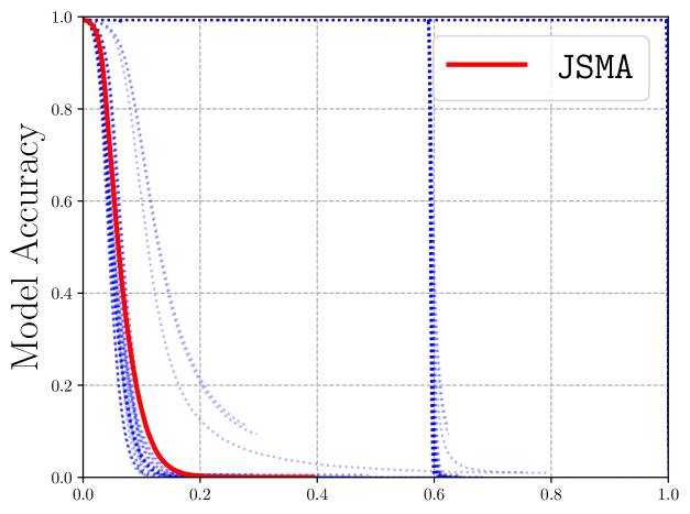
(a) $\ell_{0}$

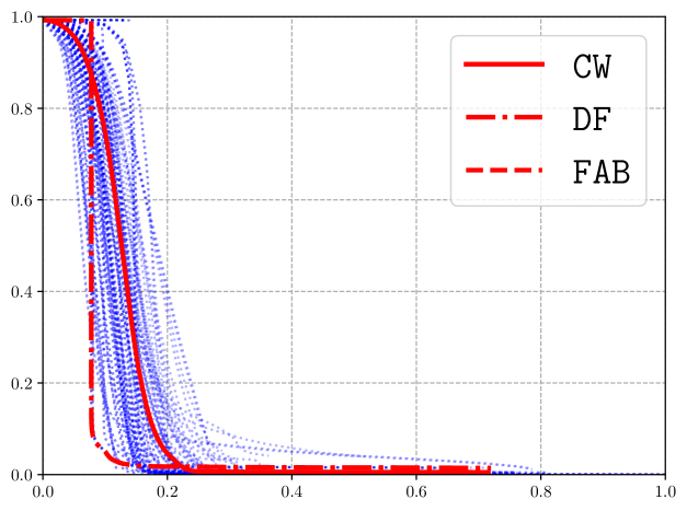
(b) $\ell_{2}$

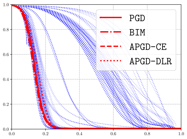
(c) $\ell_{\infty}$

Figure 3: MNIST model accuracy for (normalized) $\ell_{0}$-, $\ell_{2}$-, and $\ell_{\infty}$-based budgets. Known attacks are highlighted in red. Results show median accuracy across $1000$ iterations over $10$ trials.

$\ell_{0}$ Attacks. Figure 3 shows $\ell_{0}$-targeted attack performance with the JSMA in red. We observe that the JSMA is worse than most attacks. Attack performance is largely well-clustered with a few poor performing attacks near the top right portions of the graph. These attacks used Random-Restart, and thus, immediately consume most of the available $\ell_{0}$ budget.

$\ell_{2}$ Attacks. Figure 3 shows $\ell_{2}$-targeted attacks, with CW as solid red, DF as dash-dotted red, and FAB as dashed red. Like $\ell_{0}$, attacks are well-concentrated (albeit with slightly more spread). Notably, DF and FAB (which are ostensibly superimposed on one another), demonstrate impressive performance (the red lines that are nearly vertical)—both drop model accuracy with a near-zero increase in budget. CW exhibits moderate performance over the budget space.

$\ell_{\infty}$ Attacks. Figure 3 shows $\ell_{\infty}$-targeted attacks, with PGD as solid red, BIM as dash-dotted red, APGD-CE as dashed red, and APGD-DLR as dotted red. Unlike other norms, $\ell_{\infty}$ has clear separation, broadly attributable to using Change of Variables (specifically, attacks that used Change of Variables performed worse than those that did not). Finally, all of the known attacks exhibit near-identical performance, with APGD-DLR slightly pulling ahead at budgets $>0.2$.

From our norm-based analysis, we highlight that: (1) Random-Restart is largely inappropriate for $\ell_{0}$-targeted attacks (in that benefits do not outweigh the cost), (2) $\ell_{2}$-targeted attacks cluster fairly well; no individual attack substantially outperformed any other, and (3) $\ell_{\infty}$-targeted attacks were broadly unable to exploit Change of Variables.

5.2.2 Relative Performance to Known Attacks

Recall our central question for this experiment: do known attacks perform best? To answer this question, we analyze the minimum budget necessary for attacks to cause model accuracy to be $<1\text{\,}\mathrm{\char 37\relax}$ (attacks that fail to do so are encoded as consuming infinite budget). We run attacks for $1000$ iterations over ten trials and report the median results in Table 2.

$\ell_{0}$ Attacks				$\ell_{2}$ Attacks				$\ell_{\infty}$ Attacks
Rank	Attack	% Reduction	$\ell_{0}$ Budget	Rank	Attack	% Reduction	$\ell_{2}$ Budget	Rank	Attack	% Reduction	$\ell_{\infty}$ Budget
1.	ATK171	-$41\text{\,}\mathrm{\char 37\relax}$	0.10	1.	ATK460	-$50\text{\,}\mathrm{\char 37\relax}$	0.12	1.	ATK449	-$8\text{\,}\mathrm{\char 37\relax}$	0.22
30.	JSMA	—	0.17	69.	CW	—	0.24	17.	APGD-DLR	—	0.24
68.	ATK246	+$352\text{\,}\mathrm{\char 37\relax}$	0.77	88.	ATK37	+$45\text{\,}\mathrm{\char 37\relax}$	0.35	40.	BIM	+$16\text{\,}\mathrm{\char 37\relax}$	0.28
				136.	DF	$+\infty\%$	$\infty$	48.	APGD-CE	+$20\text{\,}\mathrm{\char 37\relax}$	0.29
				137.	FAB	$+\infty\%$	$\infty$	49.	PGD	+$20\text{\,}\mathrm{\char 37\relax}$	0.29
								135.	ATK191	+$304\text{\,}\mathrm{\char 37\relax}$	0.97

Table 2: MNIST Relative Attack Comparisons. Budgets are normalized. Attacks that fail to reduce model accuracy to be $<1\text{\,}\mathrm{\char 37\relax}$ are labeled as consuming infinite budget. Budget reductions are relative to the best known attack for each $\ell_{p}$-norm.

Here, attacks are ranked by budget and segmented by norm (i.e., $192$ attacks per norm). We report the percentage change of each attack with respect to the known attack that performed best in that norm (that is, for $\ell_{0}$, results are relative to the JSMA, while for $\ell_{2}$, results are relative to CW, which outperformed DF, etc.). In the table, we show: (1) the attack that ranked first, (2) ranks of known attacks, and (3) the lowest ranked attack that still reduced model accuracy to $<1\text{\,}\mathrm{\char 37\relax}$. Next, we highlight some strong trends for each $\ell_{p}$-norm.

Of the $34\text{\,}\mathrm{\char 37\relax}$ of attacks that succeed in the $\ell_{0}$ space, the JSMA (ranked $32^{\mathrm{nd}}$) was at the bottom of the highly performant bin (in that its $\ell_{0}$ budget was $0.17$)—the JSMA was held back by its saliency map, SM_J; using either SM_D (or no saliency map at all, i.e., SM_I) was almost always better. While CW seemingly rank low (i.e., $69^{\mathrm{th}}$), we note that $\ell_{2}$ budgets were broadly similar, as the worst and best performing attacks were within $\pm$$50\text{\,}\mathrm{\char 37\relax}$ of the budget consumed by CW. APGD-DLR, BIM, APGD-CE, and PGD, ranked $17^{\mathrm{th}}$, $40^{\mathrm{th}}$, $48^{\mathrm{th}}$, and $49^{\mathrm{th}}$ respectively, were marginally outperformed by attacks using either the SM_D saliency map or BWSGD optimizer. As a final note, we were confounded by the performance of DF and FAB—visually inspecting Figure 3, both are clearly superior attacks (the performance curves ostensibly resemble square waves) and yet, they failed to reduce model accuracy to $<1\text{\,}\mathrm{\char 37\relax}$. While these analyses of attack performance has been useful historically for understanding adversarial examples, we argue that this “race to $0\text{\,}\mathrm{\char 37\relax}$ accuracy” fails to capture meaningful definitions of attack performance (as made evident by the apparent “failure” of DF and FAB).

From our comparison with known attacks, we highlight two key takeaways: (1) Measuring the required distortion to reach some amount of model accuracy is a rather crude approach to estimating attack performance. We argue using measurements that factor the entire budget space (such as the PEA, which we use subsequently) will yield more meaningful interpretations of attack performance. (2) Even when we define success as $<1\text{\,}\mathrm{\char 37\relax}$ model accuracy, known attacks do not perform best. In fact, many attacks produced by our decomposition consistently outperformed known attacks (e.g., $68$ out of the $189$ introduced by our approach outperformed both CW and DF), which demonstrates the novel adversarial capabilities introduced by our decomposition.

Figure 4: Median Spearman Rank Correlation Coefficients for MNIST—Results are segmented by $\ell_{p}$-norm. Data points correspond to a specific threat model (i.e., a value for $\theta$). High attack performance generalization is encoded as lighter shades, while low generalization is encoded with darker shades. Top row shows within-norm generalization & bottom row shows cross-norm generalization.

5.3 Optimal Attacks

In subsection 4.2, we introduced an approach for measuring optimality: the area between the performance curves of the PEA and an attack. Attacks that have a small area closely track the PEA and thus, are performant attacks, while those that have a large area perform poorly. In this experiment, we ask: does attack performance generalize? In other words, is relative attack performance invariant to dataset or threat model?

We investigate this hypothesis of attack optimality by ranking attacks by area across varying threat models, datasets, and robust models. Then, we measure the generalization of these rankings via the Spearman rank correlation coefficient [51], which informs us how similar the rankings are between two datasets, threat models, or a robust and non-robust model.

For example, a highly positive correlation across two datasets would imply that relative attack performance was unchanged (in other words, changing the dataset had little to no effect on attack performance), a near-zero correlation would suggest that relative attack performance changed substantially (which would suggest attack performance is sensitive to the dataset), and a negative correlation would indicate attack performance was reversed (i.e., the worst attacks on one dataset became the best on another). In our experiments, we craft adversarial examples for $1000$ iterations over ten trials and report the median Spearman rank correlation coefficients. We note that $1000$ iterations was selected for completeness; the vast majority of attacks converged in less than $100$ iterations.

Optimal Attacks by Threat Model. Here, we analyze the generalization of attack performance across threat models. Specifically, we consider $\ell_{0}$-, $\ell_{2}$-, and $\ell_{\infty}$-based threat models with varying values of $\theta$ (from $02$). Note that $\theta=0$ (i.e., where compute time is ignored) is the commonly used threat model. Figure 4 shows the median Spearman rank correlation coefficients for MNIST (other datasets are listed in appendix C)with results segmented by $\ell_{p}$-norm. Each entry corresponds to a unique threat model (i.e., a value for $\theta$). High attack performance generalization is encoded as lighter shades, while low generalization is encoded with darker shades.

From the results, we can readily observe: (1) rankings do not generalize across $\ell_{p}$-norms, especially between $\ell_{0}$- and $\ell_{\infty}$-targeted attacks (but do generalize relatively well within an $\ell_{p}$-norm), and (2) the influence of compute on rankings appears to be $\ell_{p}$-norm dependent: $\ell_{0}$-based threat models that weight compute (i.e., $\theta\neq 0$) do not generalize well to those that do not, $\ell_{2}$-based threat models exhibit a smoother degradation of generalization, while, surprisingly, $\ell_{\infty}$-based threat models generalize everywhere (that is, the same attacks that were found to be performant with $\theta=2$ were as performant when $\theta=0$). Within a dataset, we observe that the threat model significantly affects attack performance across $\ell_{p}$-norms, and to some extent, within an $\ell_{p}$-norm, with $\ell_{\infty}$ as the exception.

Optimal Attacks by Dataset. In this experiment, we instead now measure the generalization of attack performance across datasets. Specifically, for a given threat model, we measure the generalization of attack performance rankings across seven datasets. The evaluated datasets span varying forms of phenomena, from classifying network traffic to categorizing clothing items, and thus, we investigate if performant attacks are task-agnostic. Correlations for threat models with $0<\theta<2$ can be found in appendix C.

The results in Figure 5 disclose that: (1) CIFAR-10 does not generalize at all, regardless of $\ell_{p}$-norm, (2) skewing budgets towards favoring compute gradually degrades generalization—attack rankings become increasingly dissimilar as we move from ignoring compute time ($\theta=0$) to heavily favoring it ($\theta=2$), and (3) $\ell_{0}$-based threat models readily generalize across datasets and is largely invariant to considering compute, $\ell_{2}$ attacks, regardless of $\theta$, moderately generalize, and $\ell_{\infty}$ attacks closely track $\ell_{2}$ attacks with a particular subtly: attacks performant on MNIST generalized almost perfectly to FMNIST (i.e., image-based generalization), while attacks performant on NSL-KDD almost perfectly generalized to UNSW-NB15 (i.e., network-intrusion-detection-based generalization). Lastly, we observe that attacks performant on Phishing and MalMem moderately generalized better to non-image data (particularly to the UNSW-NB15). Considering compute degrades these observations slightly. Within a threat model, we observe that, based on $\ell_{p}$-norm, the dataset can have drastic degrees of influence on attack performance, in that it can have little effect at all (e.g., $\ell_{0}$), have an effect everywhere (i.e., $\ell_{2}$), or have an effect specific to the phenomena (i.e., $\ell_{\infty}$). We attribute the unique behavior of CIFAR-10 to its dimensionality; the next largest dataset, FMNIST and MNIST, are $\sim$$74\text{\,}\mathrm{\char 37\relax}$ smaller.

Optimal Attacks Against Robust Models. In this final experiment, we now measure the generalization of attack performance between robust and non-robust models. Specifically, for a given threat model and dataset, we compute pairwise correlations between attack performance rankings on robust and non-robust models. Adversarially trained models have been shown to be an effective defense against adversarial examples [33], and thus, we investigate if such procedures have a visible effect on attack performance.

Median Spearman rank correlation coefficients for all datasets and threat models are shown in Figure 6. We note several trends across norm, threat models, and datasets: (1) generally speaking, attack rankings in $\ell_{2}$-based threat models were substantially affected by robust models, especially for MalMem, MNIST, and FMNIST, (2) considering compute can have a significant impact on generalization, mainly dependant on the norm; increasing the importance of compute almost universally aided generalization in $\ell_{2}$, but hurt generalization in $\ell_{0}$ (especially for image data, albeit CIFAR-10 is less sensitive to varying $\theta$ at the scales we investigated), and (3) we observed that top-performing attacks can be especially affected: on MNIST for an $\ell_{2}+0\cdot\mathrm{time}$ threat model, for instance, the top $10$ attacks on the non-robust model had a median rank of $445^{th}$ (out of $576$) on the robust model. These profound differences in relative attack effectiveness demonstrate that the unique properties of robust models necessitate changes to attack components (discussed further in subsection 5.4.3).

Takeaways on Attack Optimality. In this set of experiments, we analyzed attack optimality through the lens of varying threat models, unique data phenomena, and robust models. From our analyses, we find that the optimality of any given attack is highly dependant on the given context. We support this conclusion through the following remarks on the generalization of relative attack performance: (1) across threat models, performance generalizes well within an $\ell_{p}$-norm, but not across—considering compute exacerbates this observation, (2) across datasets, performance generalization is broadly sensitive to $\ell_{p}$-norm (with CIFAR-10 generalizing poorly everywhere), and (3) between robust and non-robust models, attack rankings are largely a function of data phenomena (e.g., image-based phenomena exhibit poor generalization, regardless of the threat model).

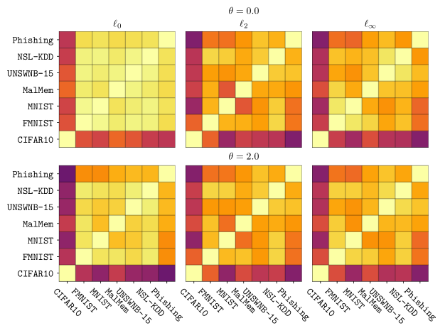
Figure 5: Median Spearman Rank Correlation Coefficients for $\theta=0$ and $\theta=2$ threat models—Results are segmented by $\ell_{p}$-norm. Entries correspond to a dataset pair. High attack performance generalization is encoded as lighter shades, while low generalization is encoded with darker shades.

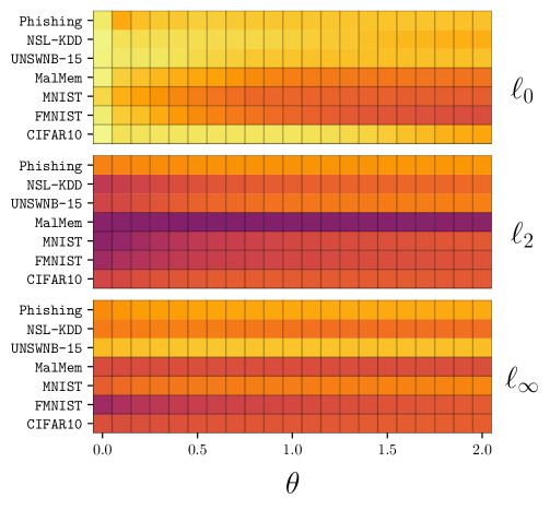
Figure 6: Median Spearman Rank Correlation Coefficients for robust and non-robust models—Results are segmented by $\ell_{p}$-norm. Data points correspond to a specific threat model (i.e., a value for $\theta$). Lighter shades show high generalization of attack performance ranking across that dataset and threat model, while darker shades are low generalization.

5.4 When and Why Attacks Perform Well

With our metric for attack performance established and evaluated, we proceed by asking, why do certain attacks perform well? Here, we explore the general trends of attack components and their influence on performance through a series of hypothesis tests. We build a space of possible hypotheses of relative attack performance (over all attack components), perform hypothesis testing against this space, and identify those with the highest significance and effect size. We begin with significant hypotheses of non-robust models and conclude with hypotheses most affected by model robustness.

5.4.1 The Space of Hypotheses

We define a hypothesis as a comparison between two component values (which we label as $H_{1}$ and $H_{2}$), such as “using Cross-Entropy is better than Carlini-Wagner Loss.” Now, we want to understand the conditions that make a hypothesis true. These conditions can be using a specific dataset, under a certain threat model, or based on other component values. Building off our previous example, this hypothesis paired with a condition could be “using Cross-Entropy is better than Carlini-Wagner Loss, when the dataset is Phishing.” When we test a hypothesis, we look at the statistical significance of the hypothesis under all conditions to determine when a hypothesis is true. Enumerating across all possible hypothesis and condition pairs yielded $1690$ candidate hypotheses. It should be noted that the component values in hypotheses are always in the same component, as comparing usefulness across components would be nonsensical (e.g., “Using Cross-Entropy is better than using Random-Restart” is not meaningful).

	Component $\mathbf{H_{1}}$		Component $\mathbf{H_{2}}$		Condition	$\mathbf{p}$-value	Effect Size
1.	SGD	is better than	BWSGD	when	$\mathtt{Dataset}=\texttt{MNIST}{}$	$<2.2\text{\times}{10}^{-308}$	$99\text{\,}\mathrm{\char 37\relax}$
2.	Adam	is better than	BWSGD	when	$\mathtt{Dataset}=\texttt{MNIST}{}$	$<2.2\text{\times}{10}^{-308}$	$99\text{\,}\mathrm{\char 37\relax}$
⋮				⋮
84.	Identity Loss	is better than	Difference of Logits Ratio Loss	when	$\mathtt{Dataset}=\texttt{NSL-KDD}{}$	$<2.2\text{\times}{10}^{-308}$	$93\text{\,}\mathrm{\char 37\relax}$
85.	SGD	is better than	BWSGD	when	$\mathtt{SaliencyMap}=\texttt{Jacobian Saliency Map}{}$	$<2.2\text{\times}{10}^{-308}$	$92\text{\,}\mathrm{\char 37\relax}$
⋮				⋮
393.	DeepFool Saliency Map	is better than	Jacobian Saliency Map	when	$\mathtt{Dataset}=\texttt{FMNIST}{}$	$<5\text{\times}{10}^{-6}$	$66\text{\,}\mathrm{\char 37\relax}$
394.	Cross-Entropy	is better than	Carlini-Wagner Loss	when	$\textit{Change of Variables}{}=\textit{Disabled}$	$<5\text{\times}{10}^{-6}$	$61\text{\,}\mathrm{\char 37\relax}$
⋮				⋮
1689.	$\ell_{0}$	is better than	$\ell_{2}$	when	$\mathtt{Threat\ Model}=\ell_{2}+1.0$	$9.8\text{\times}{10}^{-01}$	$50\text{\,}\mathrm{\char 37\relax}$
1690.	Identity Saliency Map	is better than	DeepFool Saliency Map	when	$\mathtt{Threat\ Model}=\ell_{\infty}+0.4$	$1.0\text{\times}{10}^{00}$	$49\text{\,}\mathrm{\char 37\relax}$

Table 3: The evaluated hypotheses for non-robust models. The top $344$ hypotheses have a $p$-value that exhibits $64\text{\,}\mathrm{bit}$ underflow. When sorted by effect size, the top $50\text{\,}\mathrm{\char 37\relax}$ of hypotheses have an effect size greater than $80\text{\,}\mathrm{\char 37\relax}$.

5.4.2 Testing

We test the $1690$ hypotheses with the Wilcoxon Signed-Rank Test, a non-parametric pairwise test, equivalent to a pairwise Mann-Whitney $U$ Test, to determine its significance. We also report the effect size of the test, defined as the percentage of pairwise median areas (over ten trials, with trial counts factored into computed $p$-values) from component $H_{1}$ that were smaller than component $H_{2}$ (recall, a smaller area corresponds to a better attack, as it more closely tracks the PEA). Note that the $p$-values for many hypotheses underflowed $64\text{\,}\mathrm{bit}$ floating point precision, implying that the results of the test are highly significant across all datasets and threat models. A subset of of hypotheses are represented in Table 3.

We find many highly-significant correlations in the results across the space of hypotheses. Specifically, we set a significance threshold proportional to the number of hypothesis tests we evaluated to minimize false positives: $p<\frac{0.01}{1690}=$5\text{\times}{10}^{-6}$$. We found that $1536$ ($90\text{\,}\mathrm{\char 37\relax}$) of hypotheses were below this threshold. We highlight the most prominent conclusions among these $1536$ hypothesis: (1) Change of Variables was found to be disadvantageous—$86$ hypotheses involving Change of Variables met our threshold; all $86$ were against its use, (2) Adam was superior to all other optimizers—$503$ hypotheses comparing Adam to other optimizers met our threshold, of which $50\text{\,}\mathrm{\char 37\relax}$ of them ruled in favor of Adam (with SGD at $33\text{\,}\mathrm{\char 37\relax}$, and MBS at $16\text{\,}\mathrm{\char 37\relax}$), (3) Random-Restart was found to be preferable across $61\text{\,}\mathrm{\char 37\relax}$ of hypotheses ($51$ of $83$), (4) $\ell_{\infty}$-targeted attacks, at $79\text{\,}\mathrm{\char 37\relax}$ ($163$ of $205$) were superior to both $\ell_{0}$- and $\ell_{2}$-targeted (which were only favorable $16\text{\,}\mathrm{\char 37\relax}$ ($34$ of $205$) and $4\text{\,}\mathrm{\char 37\relax}$ ($8$ of $205$) of the time, respectively), (5) using no saliency map (i.e., SM_I) was better $70\text{\,}\mathrm{\char 37\relax}$ ($131$ of $187$) of the time, (6) perhaps surprisingly, using no loss function was more advantageous $47\text{\,}\mathrm{\char 37\relax}$ ($224$ of $472$) of the time, over CE and CWL, which were useful $34\text{\,}\mathrm{\char 37\relax}$ ($161$ of $472$) and $18\text{\,}\mathrm{\char 37\relax}$ ($87$ of $472$) of the time, respectively, and (7) contrary to common practice, using $\ell_{\infty}$-based attacks were sometimes superior to $\ell_{2}$-based attacks for $\ell_{2}$-based threat models ($21$ of $42$); this result would suggest that perturbing based on the magnitude of gradients, while effective, can be excessive (when measuring cost under $\ell_{2}$) and unnecessary to meet adversarial goals.

We highlight some key takeaways from this experiment: (1) These hypothesis tests provide statistical evidence of some common practices within the community (using Random-Restart and the superiority of Adam), while also demonstrating some perhaps surprising conclusions, such as the detriment of using Cross-Entropy over no loss function at all. (2) We emphasize the utility of hypothesis testing for threat modeling as well: the tests provide a schema for performing worst-case benchmarks in their respective domain. For example, when benchmarking MNIST against $\ell_{0}$-based adversaries, attacks that use the Jacobian Saliency Map are likely to outperform attacks that use DeepFool Saliency Map.

5.4.3 The Effect of Model Robustness

As shown in Figure 6, robust models can have a significant impact on attack rankings. Here, we investigate why such broad phenomena occur. Specifically, we investigate how attack parameter choices change performance on a robust versus a non-robust model. We repeat our hypothesis testing on robust models only and compare the hypotheses most affected (that is, the largest changes in effect size) by robust models.

Table 4 provides a listing of the top pairs of hypotheses, sorted by the change in effect size from a non-robust to robust model (labeled as delta). Many of the top hypotheses when migrating from non-robust to robust models largely concern CIFAR-10 and MalMem, which were broadly the most unique phenomena across our experiments. Specifically, we see large changes in losses and saliency maps for the attacks that were effective at attacking robust models. The emphasis on CE could be in part attributed to the fact that both the model is trained on this loss as well as used by PGD, the attack used to generate adversarial examples within minibatches. This observation suggests that alignment between between attack losses and losses used for adversarial training is highly effective at attacking robust models.

Beyond the influence of loss on CIFAR-10 and MalMem, most of our tested hypotheses remained relatively unaffected by model robustness: of the $1690$ hypotheses tested, only $334$ had an effect size change of $10\text{\,}\mathrm{\char 37\relax}$ or greater between robust and non-robust models. This implies that, while many of the factors that make attacks effective do not vary between normally- and adversarially-trained models, the subset that does vary accounts for a vast difference in attack effectiveness.

	Component $\mathbf{H_{1}}$		Component $\mathbf{H_{2}}$		Condition	$\mathbf{p}$-value	Effect Size	Delta
1.	Cross-Entropy	is better than	Difference of Logits Ratio Loss	when	$\mathtt{Dataset}=\texttt{CIFAR-10}{}$	$<2.2\text{\times}{10}^{-308}$	$96\text{\,}\mathrm{\char 37\relax}$	$45\text{\,}\mathrm{\char 37\relax}$
2.	Identity Saliency Map	is better than	DeepFool Saliency Map	when	$\mathtt{Dataset}=\texttt{CIFAR-10}{}$	$<2.2\text{\times}{10}^{-308}$	$74\text{\,}\mathrm{\char 37\relax}$	$44\text{\,}\mathrm{\char 37\relax}$
3.	Difference of Logits Ratio Loss	is better than	Carlini-Wagner Loss	when	$\mathtt{Dataset}=\texttt{NSL-KDD}{}$	$<1\text{\times}{10}^{-5}$	$57\text{\,}\mathrm{\char 37\relax}$	$44\text{\,}\mathrm{\char 37\relax}$
4.	Cross-Entropy	is better than	Identity Loss	when	$\mathtt{Dataset}=\texttt{MalMem}{}$	$<2.2\text{\times}{10}^{-308}$	$69\text{\,}\mathrm{\char 37\relax}$	$43\text{\,}\mathrm{\char 37\relax}$
5.	Random-Restart: Disabled	is better than	Random-Restart: Enabled	when	$\mathtt{Optimizer}=\texttt{BWSGD}{}$	$<2.2\text{\times}{10}^{-308}$	$92\text{\,}\mathrm{\char 37\relax}$	$41\text{\,}\mathrm{\char 37\relax}$
6.	Adam	is better than	SGD	when	$\mathtt{Dataset}=\texttt{MalMem}{}$	$<1\text{\times}{10}^{-5}$	$46\text{\,}\mathrm{\char 37\relax}$	$39\text{\,}\mathrm{\char 37\relax}$
7.	Random-Restart: Disabled	is better than	Random-Restart: Enabled	when	$\mathtt{Dataset}=\texttt{MalMem}{}$	$<2.2\text{\times}{10}^{-308}$	$90\text{\,}\mathrm{\char 37\relax}$	$35\text{\,}\mathrm{\char 37\relax}$
8.	Identity Loss	is better than	Difference of Logits Ratio Loss	when	$\mathtt{Dataset}=\texttt{NSL-KDD}{}$	$<1\text{\times}{10}^{-5}$	$57\text{\,}\mathrm{\char 37\relax}$	$35\text{\,}\mathrm{\char 37\relax}$
9.	Random-Restart: Disabled	is better than	Random-Restart: Enabled	when	$\mathtt{Dataset}=\texttt{UNSW-NB15}{}$	$<1\text{\times}{10}^{-5}$	$65\text{\,}\mathrm{\char 37\relax}$	$33\text{\,}\mathrm{\char 37\relax}$
10.	Carlini-Wagner Loss	is better than	Difference of Logits Ratio Loss	when	$\mathtt{Dataset}=\texttt{CIFAR-10}{}$	$<2.2\text{\times}{10}^{-308}$	$81\text{\,}\mathrm{\char 37\relax}$	$32\text{\,}\mathrm{\char 37\relax}$
11.	Cross-Entropy	is better than	Carlini-Wagner Loss	when	$\mathtt{SaliencyMap}=\texttt{Identity Saliency Map}{}$	$<2.2\text{\times}{10}^{-308}$	$83\text{\,}\mathrm{\char 37\relax}$	$31\text{\,}\mathrm{\char 37\relax}$
12.	Cross-Entropy	is better than	Difference of Logits Ratio Loss	when	$\mathtt{Dataset}=\texttt{NSL-KDD}{}$	$6.4\text{\times}{10}^{-05}$	$55\text{\,}\mathrm{\char 37\relax}$	$31\text{\,}\mathrm{\char 37\relax}$
13.	Cross-Entropy	is better than	Identity Loss	when	$\mathtt{SaliencyMap}=\texttt{Identity Saliency Map}{}$	$<1\text{\times}{10}^{-5}$	$57\text{\,}\mathrm{\char 37\relax}$	$30\text{\,}\mathrm{\char 37\relax}$
14.	Identity Saliency Map	is better than	DeepFool Saliency Map	when	$\mathtt{Loss}=\texttt{Cross-Entropy}{}$	$<2.2\text{\times}{10}^{-308}$	$79\text{\,}\mathrm{\char 37\relax}$	$30\text{\,}\mathrm{\char 37\relax}$
15.	Identity Saliency Map	is better than	Jacobian Saliency Map	when	$\mathtt{Dataset}=\texttt{CIFAR-10}{}$	$<2.2\text{\times}{10}^{-308}$	$79\text{\,}\mathrm{\char 37\relax}$	$29\text{\,}\mathrm{\char 37\relax}$

Table 4: The top 15 hypotheses for robust models. Delta represents the difference in effect size when changing to a robust model.

6 Discussion

Domain Constraints. While adversarial machine learning research has been cast predominantly through images, the threats imposed to machine-learning-based detection systems via malware or network attacks are increasingly concerning. However, producing legitimate adversarial examples in the form of binaries or packet captures is a nuanced process; there are constraints, dictated by the domain, that adversarial examples must comply with [48, 9, 1, 59, 34, 17, 34, 56, 26].

In addition, adversarial goals in such domains are not precisely captured by subsection 2.1; attacks are commonly targeted towards a specific class (such as, classifying a variety of malicious network flows as benign traffic [49, 48, 59, 31] or malware families as legitimate software [23, 1, 16, 17, 27]). Moreover, recent work has shown the unique challenges of producing adversarial examples in the problem space [17, 16, 41]. Such works identified a set of properties input perturbations must adhere to in order to be considered demonstrative of malicious inputs in the respective problem space (e.g., packet captures or binaries), such as semantic preservation, problem-space transformations, robustness to preprocessing, among other important attributes.

These necessary factors provide a more realistic perspective on the robustness of machine learning systems in security-critical domains. While we did not explore these factors for scope, we acknowledge their importance, and encourage subsequent investigations to incorporate these factors (such as ensuring perturbations are constraint-compliant at the $\ell_{p}{}$ layer of surfaces or adapting loss functions to ensure adversarial examples are misclassified as a specific target class).

The Threat Landscape. White-box adversaries are important because they represent worst-case failure modes of machine learning systems. However, black-box adversaries have demonstrated remarkable efficacy within their limited amount of available knowledge (i.e., practical threats) [38, 25, 4, 52]. While this initial application of our framework focused on white-box adversaries for their prevalence in research, we note that there natural extensions to support black-box adversaries, such as using Backward Pass Differentiable Approximation [2] in place of the model Jacobian, or the Jacobian-based dataset augmentation [37] as a saliency map for training substitute models, among other techniques. As there are a variety of techniques for efficiently mounting black-box attacks (historically through query minimization) [38, 52, 50, 11], we see value in instantiating our framework with black-box components to understand the trade-offs between such techniques.

Related Work. A natural limitation of AutoAttack that the ensemble is fixed; while it was designed to be as diverse as possible to common failures of defenses, it may fail on defenses where an expert-designed adaptive attack would succeed. Thus, the Adaptive AutoAttack (A³) extension was introduced to combine the efficacy of AutoAttack, while dynamically adapting to new defenses [60]. A³ frames building adaptive attacks as a search problem, wherein a surrogate model is built and a “backbone” attack (e.g., FGSM, PGD, CW, among others) is greedily selected, paired with a loss function and subroutines (such as Random-Restart). A³ builds upon AutoAttack in that it enables searching through the attack design space to find the most effective adaptive attack. Our work is complementary in that we provide a broad, modular attack space, while A³ provides an approach for building adaptive attacks dynamically.

7 Conclusion

In this paper, we introduced the space of adversarial strategies. We first presented an extensible decomposition of current attacks into their core components. We subsequently constructed $568$ previously unexplored attacks by permuting these components. Through this vast attack space, we measured attack optimality via the PEA: a theoretical attack that upper-bounds attack performance. With the PEA, we studied how attack rankings change across datasets, threat models, and robust vs non-robust models. From these rankings, we described the space of hypotheses, wherein we evaluated how component choices conditionally impact attack efficacy. Our investigation revealed that attack performance is highly contextual—certain components can help (or hurt) attack performance when a specific $\ell_{p}$-norm, compute budget, domain, and even phenomena is considered. The space of adversarial strategies is rich with highly competitive attacks; meaningful evaluations need to consider the myriad of contextual factors that yield performant adversaries.

8 Acknowledgements

We would like to thank the anonymous reviewers for their insightful feedback throughout the review cycle. Additionally, we would like to thank Quinn Burke, Yohan Beugin, Rachel King, and Dave Evans for their helpful comments on earlier versions of this paper.

This research was sponsored by the Combat Capabilities Development Command Army Research Laboratory and was accomplished under Cooperative Agreement Number W911NF-13-2-0045 (ARL Cyber Security CRA). The views and conclusions contained in this document are those of the authors and should not be interpreted as representing the official policies, either expressed or implied, of the Combat Capabilities Development Command Army Research Laboratory or the U.S. Government. The U.S. Government is authorized to reproduce and distribute reprints for Government purposes not withstanding any copyright notation here on. This material is based upon work supported by the National Science Foundation under Grant No. CNS-1805310 and the U.S. Army Research Laboratory and the U.S. Army Research Office under Grant No. W911NF-19-1-0374.

Appendix A Attack Encoding

Here we provide Appendix A for translating attack numbers to component values.

ATK#	Opt.	CoV	RR	$\ell_{p}$	SM	Loss
0	SGD	False	False	$\ell_{0}$	SMI	IL
1	SGD	False	False	$\ell_{2}$	SMI	IL
2	SGD	False	False	$\ell_{\infty}$	SMI	IL
JSMA	SGD	False	False	$\ell_{0}$	SMJ	IL
4	SGD	False	False	$\ell_{2}$	SMJ	IL
5	SGD	False	False	$\ell_{\infty}$	SMJ	IL
6	SGD	False	False	$\ell_{0}$	SMD	IL
DF	SGD	False	False	$\ell_{2}$	SMD	IL
8	SGD	False	False	$\ell_{\infty}$	SMD	IL
9	SGD	False	False	$\ell_{0}$	SMI	CE
10	SGD	False	False	$\ell_{2}$	SMI	CE
BIM	SGD	False	False	$\ell_{\infty}$	SMI	CE
12	SGD	False	False	$\ell_{0}$	SMJ	CE
13	SGD	False	False	$\ell_{2}$	SMJ	CE
14	SGD	False	False	$\ell_{\infty}$	SMJ	CE
15	SGD	False	False	$\ell_{0}$	SMD	CE
16	SGD	False	False	$\ell_{2}$	SMD	CE
17	SGD	False	False	$\ell_{\infty}$	SMD	CE
18	SGD	False	False	$\ell_{0}$	SMI	CWL
19	SGD	False	False	$\ell_{2}$	SMI	CWL
20	SGD	False	False	$\ell_{\infty}$	SMI	CWL
21	SGD	False	False	$\ell_{0}$	SMJ	CWL
22	SGD	False	False	$\ell_{2}$	SMJ	CWL
23	SGD	False	False	$\ell_{\infty}$	SMJ	CWL
24	SGD	False	False	$\ell_{0}$	SMD	CWL
25	SGD	False	False	$\ell_{2}$	SMD	CWL
26	SGD	False	False	$\ell_{\infty}$	SMD	CWL
27	SGD	False	False	$\ell_{0}$	SMI	DLR
28	SGD	False	False	$\ell_{2}$	SMI	DLR
29	SGD	False	False	$\ell_{\infty}$	SMI	DLR
30	SGD	False	False	$\ell_{0}$	SMJ	DLR
31	SGD	False	False	$\ell_{2}$	SMJ	DLR
32	SGD	False	False	$\ell_{\infty}$	SMJ	DLR
33	SGD	False	False	$\ell_{0}$	SMD	DLR
34	SGD	False	False	$\ell_{2}$	SMD	DLR
35	SGD	False	False	$\ell_{\infty}$	SMD	DLR
36	SGD	True	False	$\ell_{0}$	SMI	IL
37	SGD	True	False	$\ell_{2}$	SMI	IL
38	SGD	True	False	$\ell_{\infty}$	SMI	IL
39	SGD	True	False	$\ell_{0}$	SMJ	IL
40	SGD	True	False	$\ell_{2}$	SMJ	IL
41	SGD	True	False	$\ell_{\infty}$	SMJ	IL
42	SGD	True	False	$\ell_{0}$	SMD	IL
43	SGD	True	False	$\ell_{2}$	SMD	IL
44	SGD	True	False	$\ell_{\infty}$	SMD	IL
45	SGD	True	False	$\ell_{0}$	SMI	CE
46	SGD	True	False	$\ell_{2}$	SMI	CE
47	SGD	True	False	$\ell_{\infty}$	SMI	CE
48	SGD	True	False	$\ell_{0}$	SMJ	CE
49	SGD	True	False	$\ell_{2}$	SMJ	CE
50	SGD	True	False	$\ell_{\infty}$	SMJ	CE
51	SGD	True	False	$\ell_{0}$	SMD	CE
52	SGD	True	False	$\ell_{2}$	SMD	CE
53	SGD	True	False	$\ell_{\infty}$	SMD	CE
54	SGD	True	False	$\ell_{0}$	SMI	CWL
55	SGD	True	False	$\ell_{2}$	SMI	CWL
56	SGD	True	False	$\ell_{\infty}$	SMI	CWL
57	SGD	True	False	$\ell_{0}$	SMJ	CWL
58	SGD	True	False	$\ell_{2}$	SMJ	CWL
59	SGD	True	False	$\ell_{\infty}$	SMJ	CWL
60	SGD	True	False	$\ell_{0}$	SMD	CWL
61	SGD	True	False	$\ell_{2}$	SMD	CWL
62	SGD	True	False	$\ell_{\infty}$	SMD	CWL
63	SGD	True	False	$\ell_{0}$	SMI	DLR
64	SGD	True	False	$\ell_{2}$	SMI	DLR
65	SGD	True	False	$\ell_{\infty}$	SMI	DLR
66	SGD	True	False	$\ell_{0}$	SMJ	DLR
67	SGD	True	False	$\ell_{2}$	SMJ	DLR
68	SGD	True	False	$\ell_{\infty}$	SMJ	DLR
69	SGD	True	False	$\ell_{0}$	SMD	DLR
70	SGD	True	False	$\ell_{2}$	SMD	DLR
71	SGD	True	False	$\ell_{\infty}$	SMD	DLR
72	SGD	False	True	$\ell_{0}$	SMI	IL
73	SGD	False	True	$\ell_{2}$	SMI	IL
74	SGD	False	True	$\ell_{\infty}$	SMI	IL
75	SGD	False	True	$\ell_{0}$	SMJ	IL
76	SGD	False	True	$\ell_{2}$	SMJ	IL
77	SGD	False	True	$\ell_{\infty}$	SMJ	IL
78	SGD	False	True	$\ell_{0}$	SMD	IL
79	SGD	False	True	$\ell_{2}$	SMD	IL
80	SGD	False	True	$\ell_{\infty}$	SMD	IL
81	SGD	False	True	$\ell_{0}$	SMI	CE
82	SGD	False	True	$\ell_{2}$	SMI	CE
PGD	SGD	False	True	$\ell_{\infty}$	SMI	CE
84	SGD	False	True	$\ell_{0}$	SMJ	CE
85	SGD	False	True	$\ell_{2}$	SMJ	CE
86	SGD	False	True	$\ell_{\infty}$	SMJ	CE
87	SGD	False	True	$\ell_{0}$	SMD	CE
88	SGD	False	True	$\ell_{2}$	SMD	CE
89	SGD	False	True	$\ell_{\infty}$	SMD	CE
90	SGD	False	True	$\ell_{0}$	SMI	CWL
91	SGD	False	True	$\ell_{2}$	SMI	CWL
92	SGD	False	True	$\ell_{\infty}$	SMI	CWL
93	SGD	False	True	$\ell_{0}$	SMJ	CWL
94	SGD	False	True	$\ell_{2}$	SMJ	CWL
95	SGD	False	True	$\ell_{\infty}$	SMJ	CWL

Table 5: Attack Name Encodings.

Appendix B Comparison to Known Attacks

Here we provide the full version of Table 2.

$\ell_{0}$ Attacks				$\ell_{2}$ Attacks				$\ell_{\infty}$ Attacks
Rank	Attack	% Reduction	$\ell_{0}$ Budget	Rank	Attack	% Reduction	$\ell_{2}$ Budget	Rank	Attack	% Reduction	$\ell_{\infty}$ Budget
1.	ATK171	-$41\text{\,}\mathrm{\char 37\relax}$	0.10	1.	ATK460	-$50\text{\,}\mathrm{\char 37\relax}$	0.12	1.	ATK449	-$8\text{\,}\mathrm{\char 37\relax}$	0.22
2.	ATK27	-$41\text{\,}\mathrm{\char 37\relax}$	0.10	2.	ATK532	-$50\text{\,}\mathrm{\char 37\relax}$	0.12	2.	ATK440	-$8\text{\,}\mathrm{\char 37\relax}$	0.22
3.	ATK459	-$41\text{\,}\mathrm{\char 37\relax}$	0.10	3.	ATK454	-$45\text{\,}\mathrm{\char 37\relax}$	0.13	3.	ATK17	-$8\text{\,}\mathrm{\char 37\relax}$	0.22
4.	ATK144	-$41\text{\,}\mathrm{\char 37\relax}$	0.10	4.	ATK526	-$45\text{\,}\mathrm{\char 37\relax}$	0.13	4.	ATK8	-$8\text{\,}\mathrm{\char 37\relax}$	0.22
5.	ATK150	-$41\text{\,}\mathrm{\char 37\relax}$	0.10	5.	ATK451	-$41\text{\,}\mathrm{\char 37\relax}$	0.14	5.	ATK458	-$4\text{\,}\mathrm{\char 37\relax}$	0.23
6.	ATK159	-$41\text{\,}\mathrm{\char 37\relax}$	0.10	6.	ATK523	-$41\text{\,}\mathrm{\char 37\relax}$	0.14	6.	ATK512	-$4\text{\,}\mathrm{\char 37\relax}$	0.23
7.	ATK168	-$41\text{\,}\mathrm{\char 37\relax}$	0.10	7.	ATK505	-$37\text{\,}\mathrm{\char 37\relax}$	0.15	7.	ATK521	-$4\text{\,}\mathrm{\char 37\relax}$	0.23
8.	ATK162	-$35\text{\,}\mathrm{\char 37\relax}$	0.11	8.	ATK433	-$37\text{\,}\mathrm{\char 37\relax}$	0.15	8.	ATK89	-$4\text{\,}\mathrm{\char 37\relax}$	0.23
9.	ATK153	-$29\text{\,}\mathrm{\char 37\relax}$	0.12	9.	ATK22	-$33\text{\,}\mathrm{\char 37\relax}$	0.16	9.	ATK80	-$4\text{\,}\mathrm{\char 37\relax}$	0.23
10.	ATK156	-$29\text{\,}\mathrm{\char 37\relax}$	0.12	10.	ATK94	-$33\text{\,}\mathrm{\char 37\relax}$	0.16	10.	ATK26	-$4\text{\,}\mathrm{\char 37\relax}$	0.23
11.	ATK0	-$29\text{\,}\mathrm{\char 37\relax}$	0.12	11.	ATK160	-$33\text{\,}\mathrm{\char 37\relax}$	0.16	11.	ATK461	-$4\text{\,}\mathrm{\char 37\relax}$	0.23
12.	ATK432	-$23\text{\,}\mathrm{\char 37\relax}$	0.13	12.	ATK151	-$33\text{\,}\mathrm{\char 37\relax}$	0.16	12.	ATK530	+$0\text{\,}\mathrm{\char 37\relax}$	0.24
13.	ATK24	-$23\text{\,}\mathrm{\char 37\relax}$	0.13	13.	ATK223	-$33\text{\,}\mathrm{\char 37\relax}$	0.16	13.	ATK98	+$0\text{\,}\mathrm{\char 37\relax}$	0.24
14.	ATK6	-$23\text{\,}\mathrm{\char 37\relax}$	0.13	14.	ATK232	-$33\text{\,}\mathrm{\char 37\relax}$	0.16	14.	ATK2	+$0\text{\,}\mathrm{\char 37\relax}$	0.24
15.	ATK15	-$23\text{\,}\mathrm{\char 37\relax}$	0.13	15.	ATK436	-$33\text{\,}\mathrm{\char 37\relax}$	0.16	15.	ATK29	+$0\text{\,}\mathrm{\char 37\relax}$	0.24
16.	ATK147	-$23\text{\,}\mathrm{\char 37\relax}$	0.13	16.	ATK508	-$33\text{\,}\mathrm{\char 37\relax}$	0.16	16.	ATK434	+$0\text{\,}\mathrm{\char 37\relax}$	0.24
17.	ATK456	-$23\text{\,}\mathrm{\char 37\relax}$	0.13	17.	ATK169	-$33\text{\,}\mathrm{\char 37\relax}$	0.16	17.	APGD-DLR	—	0.24
18.	ATK165	-$23\text{\,}\mathrm{\char 37\relax}$	0.13	18.	ATK277	-$29\text{\,}\mathrm{\char 37\relax}$	0.17	18.	ATK101	+$4\text{\,}\mathrm{\char 37\relax}$	0.25
19.	ATK438	-$23\text{\,}\mathrm{\char 37\relax}$	0.13	19.	ATK241	-$29\text{\,}\mathrm{\char 37\relax}$	0.17	19.	ATK74	+$4\text{\,}\mathrm{\char 37\relax}$	0.25
20.	ATK447	-$23\text{\,}\mathrm{\char 37\relax}$	0.13	20.	ATK268	-$29\text{\,}\mathrm{\char 37\relax}$	0.17	20.	ATK506	+$4\text{\,}\mathrm{\char 37\relax}$	0.25
21.	ATK177	-$17\text{\,}\mathrm{\char 37\relax}$	0.14	21.	ATK259	-$29\text{\,}\mathrm{\char 37\relax}$	0.17	21.	ATK224	+$8\text{\,}\mathrm{\char 37\relax}$	0.26
22.	ATK9	-$11\text{\,}\mathrm{\char 37\relax}$	0.15	22.	ATK187	-$29\text{\,}\mathrm{\char 37\relax}$	0.17	22.	ATK233	+$8\text{\,}\mathrm{\char 37\relax}$	0.26
23.	ATK441	-$11\text{\,}\mathrm{\char 37\relax}$	0.15	23.	ATK196	-$29\text{\,}\mathrm{\char 37\relax}$	0.17	23.	ATK170	+$8\text{\,}\mathrm{\char 37\relax}$	0.26
24.	ATK18	-$11\text{\,}\mathrm{\char 37\relax}$	0.15	24.	ATK163	-$29\text{\,}\mathrm{\char 37\relax}$	0.17	24.	ATK161	+$8\text{\,}\mathrm{\char 37\relax}$	0.26
25.	ATK450	-$11\text{\,}\mathrm{\char 37\relax}$	0.15	25.	ATK166	-$29\text{\,}\mathrm{\char 37\relax}$	0.17	25.	ATK152	+$8\text{\,}\mathrm{\char 37\relax}$	0.26
26.	ATK12	-$11\text{\,}\mathrm{\char 37\relax}$	0.15	26.	ATK28	-$29\text{\,}\mathrm{\char 37\relax}$	0.17	26.	ATK20	+$8\text{\,}\mathrm{\char 37\relax}$	0.26
27.	ATK33	-$5\text{\,}\mathrm{\char 37\relax}$	0.16	27.	ATK19	-$29\text{\,}\mathrm{\char 37\relax}$	0.17	27.	ATK455	+$8\text{\,}\mathrm{\char 37\relax}$	0.26
28.	ATK444	+$0\text{\,}\mathrm{\char 37\relax}$	0.17	28.	ATK100	-$29\text{\,}\mathrm{\char 37\relax}$	0.17	28.	ATK452	+$8\text{\,}\mathrm{\char 37\relax}$	0.26
29.	ATK465	+$0\text{\,}\mathrm{\char 37\relax}$	0.17	29.	ATK1	-$29\text{\,}\mathrm{\char 37\relax}$	0.17	29.	ATK95	+$12\text{\,}\mathrm{\char 37\relax}$	0.27
30.	JSMA	—	0.17	30.	ATK235	-$29\text{\,}\mathrm{\char 37\relax}$	0.17	30.	ATK92	+$12\text{\,}\mathrm{\char 37\relax}$	0.27
31.	ATK21	+$0\text{\,}\mathrm{\char 37\relax}$	0.17	31.	ATK238	-$29\text{\,}\mathrm{\char 37\relax}$	0.17	31.	ATK242	+$12\text{\,}\mathrm{\char 37\relax}$	0.27
32.	ATK435	+$0\text{\,}\mathrm{\char 37\relax}$	0.17	32.	ATK205	-$29\text{\,}\mathrm{\char 37\relax}$	0.17	32.	ATK527	+$12\text{\,}\mathrm{\char 37\relax}$	0.27
33.	ATK453	+$0\text{\,}\mathrm{\char 37\relax}$	0.17	33.	ATK73	-$29\text{\,}\mathrm{\char 37\relax}$	0.17	33.	ATK524	+$12\text{\,}\mathrm{\char 37\relax}$	0.27
34.	ATK99	+$252\text{\,}\mathrm{\char 37\relax}$	0.60	34.	ATK91	-$29\text{\,}\mathrm{\char 37\relax}$	0.17	34.	ATK23	+$16\text{\,}\mathrm{\char 37\relax}$	0.28
35.	ATK243	+$252\text{\,}\mathrm{\char 37\relax}$	0.60	35.	ATK115	-$25\text{\,}\mathrm{\char 37\relax}$	0.18	35.	ATK167	+$16\text{\,}\mathrm{\char 37\relax}$	0.28
36.	ATK531	+$252\text{\,}\mathrm{\char 37\relax}$	0.60	36.	ATK124	-$25\text{\,}\mathrm{\char 37\relax}$	0.18	36.	ATK437	+$16\text{\,}\mathrm{\char 37\relax}$	0.28
37.	ATK234	+$252\text{\,}\mathrm{\char 37\relax}$	0.60	37.	ATK133	-$25\text{\,}\mathrm{\char 37\relax}$	0.18	37.	ATK5	+$16\text{\,}\mathrm{\char 37\relax}$	0.28
38.	ATK231	+$252\text{\,}\mathrm{\char 37\relax}$	0.60	38.	ATK157	-$25\text{\,}\mathrm{\char 37\relax}$	0.18	38.	ATK149	+$16\text{\,}\mathrm{\char 37\relax}$	0.28
39.	ATK225	+$252\text{\,}\mathrm{\char 37\relax}$	0.60	39.	ATK229	-$25\text{\,}\mathrm{\char 37\relax}$	0.18	39.	ATK146	+$16\text{\,}\mathrm{\char 37\relax}$	0.28
40.	ATK222	+$252\text{\,}\mathrm{\char 37\relax}$	0.60	40.	ATK274	-$20\text{\,}\mathrm{\char 37\relax}$	0.19	40.	BIM	+$16\text{\,}\mathrm{\char 37\relax}$	0.28
41.	ATK240	+$252\text{\,}\mathrm{\char 37\relax}$	0.60	41.	ATK4	-$20\text{\,}\mathrm{\char 37\relax}$	0.19	41.	ATK443	+$16\text{\,}\mathrm{\char 37\relax}$	0.28
42.	ATK216	+$252\text{\,}\mathrm{\char 37\relax}$	0.60	42.	ATK76	-$20\text{\,}\mathrm{\char 37\relax}$	0.19	42.	ATK446	+$20\text{\,}\mathrm{\char 37\relax}$	0.29
43.	ATK81	+$252\text{\,}\mathrm{\char 37\relax}$	0.60	43.	ATK265	-$20\text{\,}\mathrm{\char 37\relax}$	0.19	43.	ATK239	+$20\text{\,}\mathrm{\char 37\relax}$	0.29
44.	ATK72	+$252\text{\,}\mathrm{\char 37\relax}$	0.60	44.	ATK145	-$20\text{\,}\mathrm{\char 37\relax}$	0.19	44.	ATK518	+$20\text{\,}\mathrm{\char 37\relax}$	0.29
45.	ATK90	+$252\text{\,}\mathrm{\char 37\relax}$	0.60	45.	ATK217	-$16\text{\,}\mathrm{\char 37\relax}$	0.20	45.	ATK509	+$20\text{\,}\mathrm{\char 37\relax}$	0.29
46.	ATK96	+$252\text{\,}\mathrm{\char 37\relax}$	0.60	46.	ATK43	-$16\text{\,}\mathrm{\char 37\relax}$	0.20	46.	ATK77	+$20\text{\,}\mathrm{\char 37\relax}$	0.29
47.	ATK513	+$252\text{\,}\mathrm{\char 37\relax}$	0.60	47.	ATK52	-$16\text{\,}\mathrm{\char 37\relax}$	0.20	47.	ATK221	+$20\text{\,}\mathrm{\char 37\relax}$	0.29
48.	ATK87	+$252\text{\,}\mathrm{\char 37\relax}$	0.60	48.	ATK61	-$16\text{\,}\mathrm{\char 37\relax}$	0.20	48.	APGD-CE	+$20\text{\,}\mathrm{\char 37\relax}$	0.29
49.	ATK228	+$252\text{\,}\mathrm{\char 37\relax}$	0.60	49.	ATK148	-$16\text{\,}\mathrm{\char 37\relax}$	0.20	49.	PGD	+$20\text{\,}\mathrm{\char 37\relax}$	0.29
50.	ATK519	+$252\text{\,}\mathrm{\char 37\relax}$	0.60	50.	ATK220	-$16\text{\,}\mathrm{\char 37\relax}$	0.20	50.	ATK218	+$20\text{\,}\mathrm{\char 37\relax}$	0.29
51.	ATK78	+$252\text{\,}\mathrm{\char 37\relax}$	0.60	51.	ATK136	-$16\text{\,}\mathrm{\char 37\relax}$	0.20	51.	ATK14	+$20\text{\,}\mathrm{\char 37\relax}$	0.29
52.	ATK237	+$252\text{\,}\mathrm{\char 37\relax}$	0.60	52.	ATK64	-$12\text{\,}\mathrm{\char 37\relax}$	0.21	52.	ATK164	+$20\text{\,}\mathrm{\char 37\relax}$	0.29
53.	ATK510	+$252\text{\,}\mathrm{\char 37\relax}$	0.60	53.	ATK154	-$12\text{\,}\mathrm{\char 37\relax}$	0.21	53.	ATK86	+$25\text{\,}\mathrm{\char 37\relax}$	0.30
54.	ATK522	+$252\text{\,}\mathrm{\char 37\relax}$	0.60	54.	ATK226	-$12\text{\,}\mathrm{\char 37\relax}$	0.21	54.	ATK230	+$25\text{\,}\mathrm{\char 37\relax}$	0.30
55.	ATK504	+$252\text{\,}\mathrm{\char 37\relax}$	0.60	55.	ATK208	-$12\text{\,}\mathrm{\char 37\relax}$	0.21	55.	ATK236	+$25\text{\,}\mathrm{\char 37\relax}$	0.30
56.	ATK528	+$252\text{\,}\mathrm{\char 37\relax}$	0.60	56.	ATK271	-$12\text{\,}\mathrm{\char 37\relax}$	0.21	56.	ATK158	+$25\text{\,}\mathrm{\char 37\relax}$	0.30
57.	ATK249	+$252\text{\,}\mathrm{\char 37\relax}$	0.60	57.	ATK202	-$8\text{\,}\mathrm{\char 37\relax}$	0.22	57.	ATK155	+$45\text{\,}\mathrm{\char 37\relax}$	0.35
58.	ATK219	+$258\text{\,}\mathrm{\char 37\relax}$	0.61	58.	ATK172	-$8\text{\,}\mathrm{\char 37\relax}$	0.22	58.	ATK227	+$50\text{\,}\mathrm{\char 37\relax}$	0.36
59.	ATK84	+$258\text{\,}\mathrm{\char 37\relax}$	0.61	59.	ATK244	-$8\text{\,}\mathrm{\char 37\relax}$	0.22	59.	ATK245	+$66\text{\,}\mathrm{\char 37\relax}$	0.40
60.	ATK93	+$258\text{\,}\mathrm{\char 37\relax}$	0.61	60.	ATK280	-$8\text{\,}\mathrm{\char 37\relax}$	0.22	60.	ATK173	+$70\text{\,}\mathrm{\char 37\relax}$	0.41
61.	ATK105	+$258\text{\,}\mathrm{\char 37\relax}$	0.61	61.	ATK193	-$8\text{\,}\mathrm{\char 37\relax}$	0.22	61.	ATK536	+$120\text{\,}\mathrm{\char 37\relax}$	0.53
62.	ATK537	+$258\text{\,}\mathrm{\char 37\relax}$	0.61	62.	ATK256	-$4\text{\,}\mathrm{\char 37\relax}$	0.23	62.	ATK464	+$120\text{\,}\mathrm{\char 37\relax}$	0.53
63.	ATK516	+$258\text{\,}\mathrm{\char 37\relax}$	0.61	63.	ATK253	-$4\text{\,}\mathrm{\char 37\relax}$	0.23	63.	ATK104	+$120\text{\,}\mathrm{\char 37\relax}$	0.53
64.	ATK525	+$258\text{\,}\mathrm{\char 37\relax}$	0.61	64.	ATK178	-$4\text{\,}\mathrm{\char 37\relax}$	0.23	64.	ATK32	+$125\text{\,}\mathrm{\char 37\relax}$	0.54
65.	ATK75	+$258\text{\,}\mathrm{\char 37\relax}$	0.61	65.	ATK250	-$4\text{\,}\mathrm{\char 37\relax}$	0.23	65.	ATK467	+$133\text{\,}\mathrm{\char 37\relax}$	0.56
66.	ATK507	+$258\text{\,}\mathrm{\char 37\relax}$	0.61	66.	ATK103	-$4\text{\,}\mathrm{\char 37\relax}$	0.23	66.	ATK539	+$133\text{\,}\mathrm{\char 37\relax}$	0.56
67.	ATK246	+$352\text{\,}\mathrm{\char 37\relax}$	0.77	67.	ATK262	+$0\text{\,}\mathrm{\char 37\relax}$	0.24	67.	ATK35	+$137\text{\,}\mathrm{\char 37\relax}$	0.57
68.	ATK276	$+\infty\%$	$\infty$	68.	ATK31	+$0\text{\,}\mathrm{\char 37\relax}$	0.24	68.	ATK107	+$137\text{\,}\mathrm{\char 37\relax}$	0.57
69.	ATK270	$+\infty\%$	$\infty$	69.	CW	—	0.24	69.	ATK176	+$150\text{\,}\mathrm{\char 37\relax}$	0.60
70.	ATK273	$+\infty\%$	$\infty$	70.	ATK175	+$0\text{\,}\mathrm{\char 37\relax}$	0.24	70.	ATK248	+$150\text{\,}\mathrm{\char 37\relax}$	0.60
71.	ATK267	$+\infty\%$	$\infty$	71.	ATK247	+$0\text{\,}\mathrm{\char 37\relax}$	0.24	71.	ATK569	+$200\text{\,}\mathrm{\char 37\relax}$	0.72
72.	ATK261	$+\infty\%$	$\infty$	72.	ATK142	+$4\text{\,}\mathrm{\char 37\relax}$	0.25	72.	ATK137	+$200\text{\,}\mathrm{\char 37\relax}$	0.72
73.	ATK264	$+\infty\%$	$\infty$	73.	ATK127	+$4\text{\,}\mathrm{\char 37\relax}$	0.25	73.	ATK179	+$212\text{\,}\mathrm{\char 37\relax}$	0.75
74.	ATK285	$+\infty\%$	$\infty$	74.	ATK184	+$8\text{\,}\mathrm{\char 37\relax}$	0.26	74.	ATK251	+$212\text{\,}\mathrm{\char 37\relax}$	0.75
75.	ATK279	$+\infty\%$	$\infty$	75.	ATK190	+$8\text{\,}\mathrm{\char 37\relax}$	0.26	75.	ATK563	+$220\text{\,}\mathrm{\char 37\relax}$	0.77
76.	ATK282	$+\infty\%$	$\infty$	76.	ATK283	+$8\text{\,}\mathrm{\char 37\relax}$	0.26	76.	ATK497	+$220\text{\,}\mathrm{\char 37\relax}$	0.77
77.	ATK258	$+\infty\%$	$\infty$	77.	ATK211	+$12\text{\,}\mathrm{\char 37\relax}$	0.27	77.	ATK275	+$220\text{\,}\mathrm{\char 37\relax}$	0.77
78.	ATK252	$+\infty\%$	$\infty$	78.	ATK130	+$12\text{\,}\mathrm{\char 37\relax}$	0.27	78.	ATK131	+$220\text{\,}\mathrm{\char 37\relax}$	0.77
79.	ATK255	$+\infty\%$	$\infty$	79.	ATK109	+$12\text{\,}\mathrm{\char 37\relax}$	0.27	79.	ATK65	+$220\text{\,}\mathrm{\char 37\relax}$	0.77
80.	ATK204	$+\infty\%$	$\infty$	80.	ATK70	+$12\text{\,}\mathrm{\char 37\relax}$	0.27	80.	ATK281	+$220\text{\,}\mathrm{\char 37\relax}$	0.77
81.	ATK198	$+\infty\%$	$\infty$	81.	ATK181	+$12\text{\,}\mathrm{\char 37\relax}$	0.27	81.	ATK566	+$220\text{\,}\mathrm{\char 37\relax}$	0.77
82.	ATK201	$+\infty\%$	$\infty$	82.	ATK286	+$12\text{\,}\mathrm{\char 37\relax}$	0.27	82.	ATK266	+$220\text{\,}\mathrm{\char 37\relax}$	0.77
83.	ATK195	$+\infty\%$	$\infty$	83.	ATK112	+$20\text{\,}\mathrm{\char 37\relax}$	0.29	83.	ATK557	+$220\text{\,}\mathrm{\char 37\relax}$	0.77
84.	ATK189	$+\infty\%$	$\infty$	84.	ATK214	+$29\text{\,}\mathrm{\char 37\relax}$	0.31	84.	ATK548	+$220\text{\,}\mathrm{\char 37\relax}$	0.77
85.	ATK192	$+\infty\%$	$\infty$	85.	ATK55	+$33\text{\,}\mathrm{\char 37\relax}$	0.32	85.	ATK116	+$225\text{\,}\mathrm{\char 37\relax}$	0.78
86.	ATK213	$+\infty\%$	$\infty$	86.	ATK85	+$45\text{\,}\mathrm{\char 37\relax}$	0.35	86.	ATK125	+$225\text{\,}\mathrm{\char 37\relax}$	0.78
87.	ATK207	$+\infty\%$	$\infty$	87.	ATK13	+$45\text{\,}\mathrm{\char 37\relax}$	0.35	87.	ATK122	+$229\text{\,}\mathrm{\char 37\relax}$	0.79
88.	ATK210	$+\infty\%$	$\infty$	88.	ATK37	+$45\text{\,}\mathrm{\char 37\relax}$	0.35	88.	ATK134	+$229\text{\,}\mathrm{\char 37\relax}$	0.79
89.	ATK186	$+\infty\%$	$\infty$	89.	ATK421	$+\infty\%$	$\infty$	89.	ATK278	+$229\text{\,}\mathrm{\char 37\relax}$	0.79
90.	ATK180	$+\infty\%$	$\infty$	90.	ATK415	$+\infty\%$	$\infty$	90.	ATK269	+$229\text{\,}\mathrm{\char 37\relax}$	0.79
91.	ATK183	$+\infty\%$	$\infty$	91.	ATK418	$+\infty\%$	$\infty$	91.	ATK260	+$229\text{\,}\mathrm{\char 37\relax}$	0.79
92.	ATK174	$+\infty\%$	$\infty$	92.	ATK412	$+\infty\%$	$\infty$	92.	ATK554	+$233\text{\,}\mathrm{\char 37\relax}$	0.80
93.	ATK420	$+\infty\%$	$\infty$	93.	ATK406	$+\infty\%$	$\infty$	93.	ATK257	+$233\text{\,}\mathrm{\char 37\relax}$	0.80
94.	ATK414	$+\infty\%$	$\infty$	94.	ATK409	$+\infty\%$	$\infty$	94.	ATK542	+$233\text{\,}\mathrm{\char 37\relax}$	0.80
95.	ATK417	$+\infty\%$	$\infty$	95.	ATK430	$+\infty\%$	$\infty$	95.	ATK110	+$233\text{\,}\mathrm{\char 37\relax}$	0.80
96.	ATK411	$+\infty\%$	$\infty$	96.	ATK424	$+\infty\%$	$\infty$	96.	ATK254	+$233\text{\,}\mathrm{\char 37\relax}$	0.80

$\ell_{0}$ Attacks				$\ell_{2}$ Attacks				$\ell_{\infty}$ Attacks
Rank	Attack	% Reduction	$\ell_{0}$ Budget	Rank	Attack	% Reduction	$\ell_{2}$ Budget	Rank	Attack	% Reduction	$\ell_{\infty}$ Budget
97.	ATK405	$+\infty\%$	$\infty$	97.	ATK427	$+\infty\%$	$\infty$	97.	ATK545	+$237\text{\,}\mathrm{\char 37\relax}$	0.81
98.	ATK408	$+\infty\%$	$\infty$	98.	ATK403	$+\infty\%$	$\infty$	98.	ATK113	+$237\text{\,}\mathrm{\char 37\relax}$	0.81
99.	ATK429	$+\infty\%$	$\infty$	99.	ATK397	$+\infty\%$	$\infty$	99.	ATK209	+$237\text{\,}\mathrm{\char 37\relax}$	0.81
100.	ATK423	$+\infty\%$	$\infty$	100.	ATK400	$+\infty\%$	$\infty$	100.	ATK560	+$241\text{\,}\mathrm{\char 37\relax}$	0.82
101.	ATK426	$+\infty\%$	$\infty$	101.	ATK385	$+\infty\%$	$\infty$	101.	ATK272	+$241\text{\,}\mathrm{\char 37\relax}$	0.82
102.	ATK402	$+\infty\%$	$\infty$	102.	ATK379	$+\infty\%$	$\infty$	102.	ATK128	+$241\text{\,}\mathrm{\char 37\relax}$	0.82
103.	ATK396	$+\infty\%$	$\infty$	103.	ATK382	$+\infty\%$	$\infty$	103.	ATK551	+$258\text{\,}\mathrm{\char 37\relax}$	0.86
104.	ATK399	$+\infty\%$	$\infty$	104.	ATK376	$+\infty\%$	$\infty$	104.	ATK263	+$258\text{\,}\mathrm{\char 37\relax}$	0.86
105.	ATK384	$+\infty\%$	$\infty$	105.	ATK370	$+\infty\%$	$\infty$	105.	ATK119	+$258\text{\,}\mathrm{\char 37\relax}$	0.86
106.	ATK378	$+\infty\%$	$\infty$	106.	ATK373	$+\infty\%$	$\infty$	106.	ATK491	+$275\text{\,}\mathrm{\char 37\relax}$	0.90
107.	ATK381	$+\infty\%$	$\infty$	107.	ATK394	$+\infty\%$	$\infty$	107.	ATK59	+$275\text{\,}\mathrm{\char 37\relax}$	0.90
108.	ATK375	$+\infty\%$	$\infty$	108.	ATK388	$+\infty\%$	$\infty$	108.	ATK482	+$279\text{\,}\mathrm{\char 37\relax}$	0.91
109.	ATK369	$+\infty\%$	$\infty$	109.	ATK391	$+\infty\%$	$\infty$	109.	ATK50	+$279\text{\,}\mathrm{\char 37\relax}$	0.91
110.	ATK372	$+\infty\%$	$\infty$	110.	ATK367	$+\infty\%$	$\infty$	110.	ATK203	+$279\text{\,}\mathrm{\char 37\relax}$	0.91
111.	ATK393	$+\infty\%$	$\infty$	111.	ATK361	$+\infty\%$	$\infty$	111.	ATK194	+$279\text{\,}\mathrm{\char 37\relax}$	0.91
112.	ATK387	$+\infty\%$	$\infty$	112.	ATK364	$+\infty\%$	$\infty$	112.	ATK140	+$287\text{\,}\mathrm{\char 37\relax}$	0.93
113.	ATK390	$+\infty\%$	$\infty$	113.	ATK349	$+\infty\%$	$\infty$	113.	ATK494	+$291\text{\,}\mathrm{\char 37\relax}$	0.94
114.	ATK366	$+\infty\%$	$\infty$	114.	ATK343	$+\infty\%$	$\infty$	114.	ATK473	+$291\text{\,}\mathrm{\char 37\relax}$	0.94
115.	ATK360	$+\infty\%$	$\infty$	115.	ATK346	$+\infty\%$	$\infty$	115.	ATK485	+$291\text{\,}\mathrm{\char 37\relax}$	0.94
116.	ATK363	$+\infty\%$	$\infty$	116.	ATK340	$+\infty\%$	$\infty$	116.	ATK476	+$291\text{\,}\mathrm{\char 37\relax}$	0.94
117.	ATK348	$+\infty\%$	$\infty$	117.	ATK334	$+\infty\%$	$\infty$	117.	ATK185	+$291\text{\,}\mathrm{\char 37\relax}$	0.94
118.	ATK342	$+\infty\%$	$\infty$	118.	ATK337	$+\infty\%$	$\infty$	118.	ATK41	+$291\text{\,}\mathrm{\char 37\relax}$	0.94
119.	ATK345	$+\infty\%$	$\infty$	119.	ATK358	$+\infty\%$	$\infty$	119.	ATK62	+$295\text{\,}\mathrm{\char 37\relax}$	0.95
120.	ATK339	$+\infty\%$	$\infty$	120.	ATK352	$+\infty\%$	$\infty$	120.	ATK53	+$295\text{\,}\mathrm{\char 37\relax}$	0.95
121.	ATK333	$+\infty\%$	$\infty$	121.	ATK355	$+\infty\%$	$\infty$	121.	ATK44	+$295\text{\,}\mathrm{\char 37\relax}$	0.95
122.	ATK336	$+\infty\%$	$\infty$	122.	ATK331	$+\infty\%$	$\infty$	122.	ATK206	+$295\text{\,}\mathrm{\char 37\relax}$	0.95
123.	ATK357	$+\infty\%$	$\infty$	123.	ATK325	$+\infty\%$	$\infty$	123.	ATK197	+$295\text{\,}\mathrm{\char 37\relax}$	0.95
124.	ATK351	$+\infty\%$	$\infty$	124.	ATK328	$+\infty\%$	$\infty$	124.	ATK188	+$295\text{\,}\mathrm{\char 37\relax}$	0.95
125.	ATK354	$+\infty\%$	$\infty$	125.	ATK313	$+\infty\%$	$\infty$	125.	ATK284	+$300\text{\,}\mathrm{\char 37\relax}$	0.96
126.	ATK330	$+\infty\%$	$\infty$	126.	ATK307	$+\infty\%$	$\infty$	126.	ATK470	+$300\text{\,}\mathrm{\char 37\relax}$	0.96
127.	ATK324	$+\infty\%$	$\infty$	127.	ATK310	$+\infty\%$	$\infty$	127.	ATK488	+$300\text{\,}\mathrm{\char 37\relax}$	0.96
128.	ATK327	$+\infty\%$	$\infty$	128.	ATK304	$+\infty\%$	$\infty$	128.	ATK56	+$300\text{\,}\mathrm{\char 37\relax}$	0.96
129.	ATK312	$+\infty\%$	$\infty$	129.	ATK298	$+\infty\%$	$\infty$	129.	ATK38	+$300\text{\,}\mathrm{\char 37\relax}$	0.96
130.	ATK306	$+\infty\%$	$\infty$	130.	ATK301	$+\infty\%$	$\infty$	130.	ATK200	+$300\text{\,}\mathrm{\char 37\relax}$	0.96
131.	ATK309	$+\infty\%$	$\infty$	131.	ATK322	$+\infty\%$	$\infty$	131.	ATK479	+$300\text{\,}\mathrm{\char 37\relax}$	0.96
132.	ATK303	$+\infty\%$	$\infty$	132.	ATK316	$+\infty\%$	$\infty$	132.	ATK182	+$304\text{\,}\mathrm{\char 37\relax}$	0.97
133.	ATK297	$+\infty\%$	$\infty$	133.	ATK319	$+\infty\%$	$\infty$	133.	ATK212	+$304\text{\,}\mathrm{\char 37\relax}$	0.97
134.	ATK300	$+\infty\%$	$\infty$	134.	ATK289	$+\infty\%$	$\infty$	134.	ATK47	+$304\text{\,}\mathrm{\char 37\relax}$	0.97
135.	ATK321	$+\infty\%$	$\infty$	135.	ATK292	$+\infty\%$	$\infty$	135.	ATK191	+$304\text{\,}\mathrm{\char 37\relax}$	0.97
136.	ATK315	$+\infty\%$	$\infty$	136.	DF	$+\infty\%$	$\infty$	136.	ATK287	$+\infty\%$	$\infty$
137.	ATK318	$+\infty\%$	$\infty$	137.	FAB	$+\infty\%$	$\infty$	137.	ATK215	$+\infty\%$	$\infty$
138.	ATK294	$+\infty\%$	$\infty$	138.	ATK565	$+\infty\%$	$\infty$	138.	ATK422	$+\infty\%$	$\infty$
139.	ATK288	$+\infty\%$	$\infty$	139.	ATK559	$+\infty\%$	$\infty$	139.	ATK416	$+\infty\%$	$\infty$
140.	ATK291	$+\infty\%$	$\infty$	140.	ATK562	$+\infty\%$	$\infty$	140.	ATK419	$+\infty\%$	$\infty$
141.	ATK564	$+\infty\%$	$\infty$	141.	ATK556	$+\infty\%$	$\infty$	141.	ATK413	$+\infty\%$	$\infty$
142.	ATK558	$+\infty\%$	$\infty$	142.	ATK550	$+\infty\%$	$\infty$	142.	ATK407	$+\infty\%$	$\infty$
143.	ATK561	$+\infty\%$	$\infty$	143.	ATK553	$+\infty\%$	$\infty$	143.	ATK410	$+\infty\%$	$\infty$
144.	ATK555	$+\infty\%$	$\infty$	144.	ATK574	$+\infty\%$	$\infty$	144.	ATK431	$+\infty\%$	$\infty$
145.	ATK549	$+\infty\%$	$\infty$	145.	ATK568	$+\infty\%$	$\infty$	145.	ATK425	$+\infty\%$	$\infty$
146.	ATK552	$+\infty\%$	$\infty$	146.	ATK571	$+\infty\%$	$\infty$	146.	ATK428	$+\infty\%$	$\infty$
147.	ATK573	$+\infty\%$	$\infty$	147.	ATK547	$+\infty\%$	$\infty$	147.	ATK404	$+\infty\%$	$\infty$
148.	ATK567	$+\infty\%$	$\infty$	148.	ATK541	$+\infty\%$	$\infty$	148.	ATK398	$+\infty\%$	$\infty$
149.	ATK570	$+\infty\%$	$\infty$	149.	ATK544	$+\infty\%$	$\infty$	149.	ATK401	$+\infty\%$	$\infty$
150.	ATK546	$+\infty\%$	$\infty$	150.	ATK529	$+\infty\%$	$\infty$	150.	ATK386	$+\infty\%$	$\infty$
151.	ATK540	$+\infty\%$	$\infty$	151.	ATK520	$+\infty\%$	$\infty$	151.	ATK380	$+\infty\%$	$\infty$
152.	ATK543	$+\infty\%$	$\infty$	152.	ATK514	$+\infty\%$	$\infty$	152.	ATK383	$+\infty\%$	$\infty$
153.	ATK534	$+\infty\%$	$\infty$	153.	ATK517	$+\infty\%$	$\infty$	153.	ATK377	$+\infty\%$	$\infty$
154.	ATK492	$+\infty\%$	$\infty$	154.	ATK538	$+\infty\%$	$\infty$	154.	ATK371	$+\infty\%$	$\infty$
155.	ATK486	$+\infty\%$	$\infty$	155.	ATK535	$+\infty\%$	$\infty$	155.	ATK374	$+\infty\%$	$\infty$
156.	ATK489	$+\infty\%$	$\infty$	156.	ATK511	$+\infty\%$	$\infty$	156.	ATK395	$+\infty\%$	$\infty$
157.	ATK483	$+\infty\%$	$\infty$	157.	ATK493	$+\infty\%$	$\infty$	157.	ATK389	$+\infty\%$	$\infty$
158.	ATK477	$+\infty\%$	$\infty$	158.	ATK487	$+\infty\%$	$\infty$	158.	ATK392	$+\infty\%$	$\infty$
159.	ATK480	$+\infty\%$	$\infty$	159.	ATK490	$+\infty\%$	$\infty$	159.	ATK368	$+\infty\%$	$\infty$
160.	ATK501	$+\infty\%$	$\infty$	160.	ATK484	$+\infty\%$	$\infty$	160.	ATK362	$+\infty\%$	$\infty$
161.	ATK495	$+\infty\%$	$\infty$	161.	ATK478	$+\infty\%$	$\infty$	161.	ATK365	$+\infty\%$	$\infty$
162.	ATK498	$+\infty\%$	$\infty$	162.	ATK481	$+\infty\%$	$\infty$	162.	ATK350	$+\infty\%$	$\infty$
163.	ATK474	$+\infty\%$	$\infty$	163.	ATK502	$+\infty\%$	$\infty$	163.	ATK344	$+\infty\%$	$\infty$
164.	ATK468	$+\infty\%$	$\infty$	164.	ATK496	$+\infty\%$	$\infty$	164.	ATK347	$+\infty\%$	$\infty$
165.	ATK471	$+\infty\%$	$\infty$	165.	ATK499	$+\infty\%$	$\infty$	165.	ATK341	$+\infty\%$	$\infty$
166.	ATK462	$+\infty\%$	$\infty$	166.	ATK475	$+\infty\%$	$\infty$	166.	ATK335	$+\infty\%$	$\infty$
167.	ATK132	$+\infty\%$	$\infty$	167.	ATK469	$+\infty\%$	$\infty$	167.	ATK338	$+\infty\%$	$\infty$
168.	ATK126	$+\infty\%$	$\infty$	168.	ATK472	$+\infty\%$	$\infty$	168.	ATK359	$+\infty\%$	$\infty$
169.	ATK129	$+\infty\%$	$\infty$	169.	ATK457	$+\infty\%$	$\infty$	169.	ATK353	$+\infty\%$	$\infty$
170.	ATK123	$+\infty\%$	$\infty$	170.	ATK448	$+\infty\%$	$\infty$	170.	ATK356	$+\infty\%$	$\infty$
171.	ATK117	$+\infty\%$	$\infty$	171.	ATK442	$+\infty\%$	$\infty$	171.	ATK332	$+\infty\%$	$\infty$
172.	ATK120	$+\infty\%$	$\infty$	172.	ATK445	$+\infty\%$	$\infty$	172.	ATK326	$+\infty\%$	$\infty$
173.	ATK141	$+\infty\%$	$\infty$	173.	ATK466	$+\infty\%$	$\infty$	173.	ATK329	$+\infty\%$	$\infty$
174.	ATK135	$+\infty\%$	$\infty$	174.	ATK463	$+\infty\%$	$\infty$	174.	ATK314	$+\infty\%$	$\infty$
175.	ATK138	$+\infty\%$	$\infty$	175.	ATK439	$+\infty\%$	$\infty$	175.	ATK308	$+\infty\%$	$\infty$
176.	ATK114	$+\infty\%$	$\infty$	176.	ATK118	$+\infty\%$	$\infty$	176.	ATK311	$+\infty\%$	$\infty$
177.	ATK108	$+\infty\%$	$\infty$	177.	ATK121	$+\infty\%$	$\infty$	177.	ATK305	$+\infty\%$	$\infty$
178.	ATK111	$+\infty\%$	$\infty$	178.	ATK139	$+\infty\%$	$\infty$	178.	ATK299	$+\infty\%$	$\infty$
179.	ATK102	$+\infty\%$	$\infty$	179.	ATK97	$+\infty\%$	$\infty$	179.	ATK302	$+\infty\%$	$\infty$
180.	ATK60	$+\infty\%$	$\infty$	180.	ATK88	$+\infty\%$	$\infty$	180.	ATK323	$+\infty\%$	$\infty$
181.	ATK54	$+\infty\%$	$\infty$	181.	ATK82	$+\infty\%$	$\infty$	181.	ATK317	$+\infty\%$	$\infty$
182.	ATK57	$+\infty\%$	$\infty$	182.	ATK106	$+\infty\%$	$\infty$	182.	ATK320	$+\infty\%$	$\infty$
183.	ATK51	$+\infty\%$	$\infty$	183.	ATK79	$+\infty\%$	$\infty$	183.	ATK296	$+\infty\%$	$\infty$
184.	ATK45	$+\infty\%$	$\infty$	184.	ATK58	$+\infty\%$	$\infty$	184.	ATK290	$+\infty\%$	$\infty$
185.	ATK48	$+\infty\%$	$\infty$	185.	ATK46	$+\infty\%$	$\infty$	185.	ATK293	$+\infty\%$	$\infty$
186.	ATK69	$+\infty\%$	$\infty$	186.	ATK49	$+\infty\%$	$\infty$	186.	ATK575	$+\infty\%$	$\infty$
187.	ATK63	$+\infty\%$	$\infty$	187.	ATK67	$+\infty\%$	$\infty$	187.	ATK572	$+\infty\%$	$\infty$
188.	ATK66	$+\infty\%$	$\infty$	188.	ATK40	$+\infty\%$	$\infty$	188.	ATK503	$+\infty\%$	$\infty$
189.	ATK42	$+\infty\%$	$\infty$	189.	ATK25	$+\infty\%$	$\infty$	189.	ATK500	$+\infty\%$	$\infty$
190.	ATK36	$+\infty\%$	$\infty$	190.	ATK16	$+\infty\%$	$\infty$	190.	ATK143	$+\infty\%$	$\infty$
191.	ATK39	$+\infty\%$	$\infty$	191.	ATK10	$+\infty\%$	$\infty$	191.	ATK71	$+\infty\%$	$\infty$
192.	ATK30	$+\infty\%$	$\infty$	192.	ATK34	$+\infty\%$	$\infty$	192.	ATK68	$+\infty\%$	$\infty$

Table 6: MNIST Relative Attack Comparisons. Budgets are normalized. Attacks that fail to reduce model accuracy to be $<1\text{\,}\mathrm{\char 37\relax}$ are labeled as consuming infinite budget. Improvements are relative to the best known attack for each $\ell_{p}$-norm.

Appendix C The Optimal Attack

Here, we show the median Spearman rank correlation coefficients for each of our datasets and threat models. For the dataset plots, results are segmented by $\ell_{p}$-norm. Data points correspond to a specific threat model (i.e., a value for $\theta$). $\theta=\left\{0.0,0.5,1.0,1.5,2.0\right\}$ are labeled for reference. High attack performance generalization is encoded as lighter shades, while low generalization is encoded with darker shades, as shown in the colobar below:

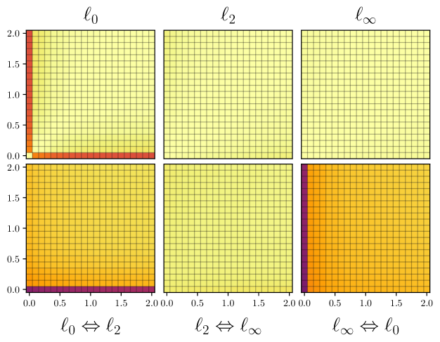
Figure 7: Phishing

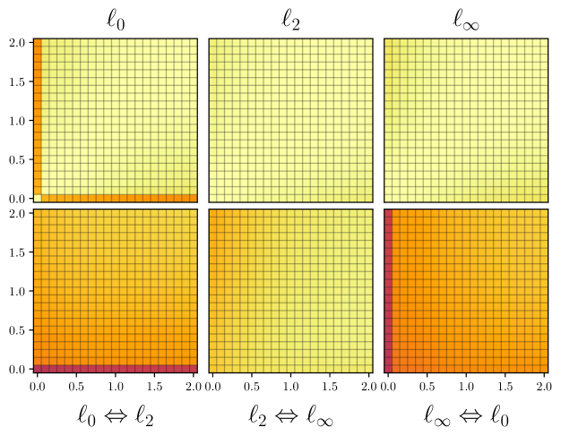
Figure 8: NSL-KDD

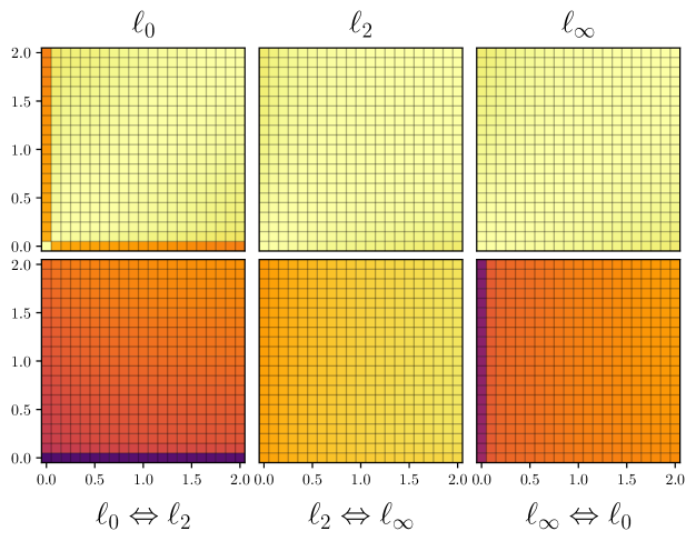
Figure 9: UNSW-NB15

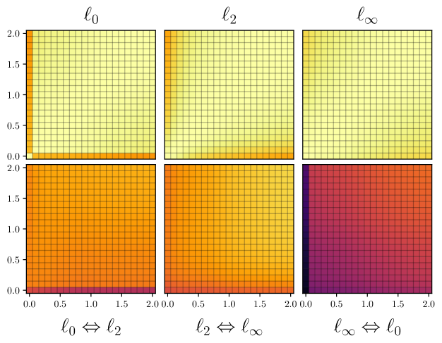
Figure 10: MNIST

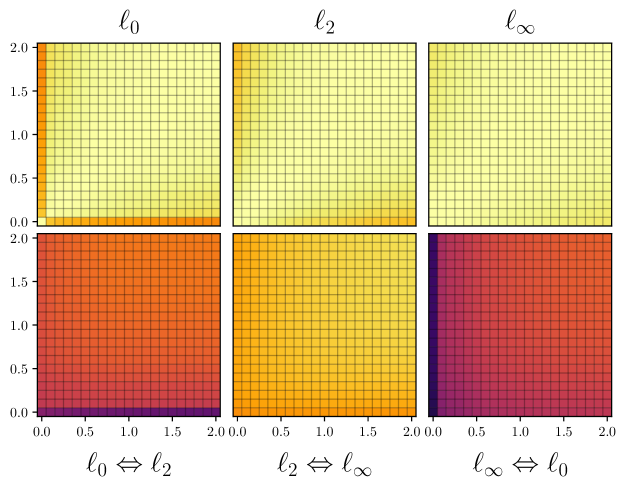
Figure 11: FMNIST

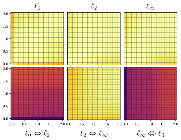
Figure 12: CIFAR-10

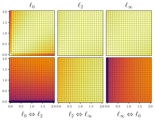
Figure 13: CIC-MalMem-2022

Appendix D Miscellany

Table 7 provides a listing of model hyperparameters for each of our datasets. Our selection was inspired by publications that report state-of-the-art accuracy for the models we used. Table 9 provides a listing of all symbols used in this paper and their associated meanings. Table 8 provides the parameters used for adversarial training.

D.1 Attack Modifications

Carlini-Wagner Attack. As described in section 3, the CW attack loss function includes a hyperparameter $c$ which controls the trade-off between the distortion introduced and misclassification. In the original attack definition, $c$ is optimized dynamically through binary-search [7]. This is cost-prohibitive and prevents us from performing any meaningful evaluation when computational cost is considered (as this attack would exist on a separate scale, when compared to PGD or even the JSMA, which requires the model Jacobian). To remedy this, we select a constant value of $c$ in our experiments. From the investigation on values of $c$ in [7] with respect to attack success probability versus mean $\ell_{2}$ distance, we choose a value of $1.0$ for $c$ in all experiments.

Jacobian-based Saliency Map Approach. The original definition of the JSMA included a search space, which defined the set of candidate features to be selected for perturbation. In the original publication, the JSMA initially set $\alpha$ to either $1$ or $0$ (that is, pixels were fully turned “off” or “on”). We find that this underestimates the performance of the JSMA on many datasets. Instead, we derive a more effective strategy of instead setting the saliency map score for some feature $i$ (in an input $x$) to $0$ if: (1) the saliency score for $i$ is positive and $x_{i}=1$, or (2) the saliency score for $i$ is negative and $x_{i}=0$. This prevents our version of the JSMA from selecting features that are already at limits of valid feature values (i.e., $1$ and $0$). Moreover, we do not select pixel pairs, as described in [39], as we found our implementation to be at least as effective (often more) as the original JSMA.

Difference of Logits Ratio Loss. The original formulation of DLR requires takes the ratio of the differences between: (1) the true logit and largest non-true-class logit, and (2) the largest logit and the third largest logit. In our evaluation, we used datasets that had less than three classes. For those scenarios, we take the second largest logit.

	Phishing	NSL-KDD	UNSW-NB15	MNIST	FMNIST	CIFAR-10	MalMem
Conv. Neurons	-	-	-	(16,32)	(16,32)	(3,64,64,128,128,256,256,	-
						256,512,512,512,512,512,)
Kernel Size	-	-	-	3	3	3	-
Stride	-	-	-	1	1	1	-
Dropout Prob.	-	-	-	0.4	0.4	0.5	-
MaxPool Kernel	-	-	-	2	2	2	-
MaxPool Stride	-	-	-	2	2	2	-
Linear Neurons	(15,)	(60,32)	(15,)	(128,)	(512,)	(512,)	(32,)
Activation	ReLU	ReLU	ReLU	ReLU	ReLU	ReLU	ReLU
Loss	CCE	CCE	CCE	CCE	CCE	CCE	CCE
Optimizer	Adam	Adam	Adam	Adam	Adam	SGD	Adam
Learning Rate	1e-2	1e-2	1e-2	1e-3	1e-3	5e-2	1e-2
Epochs	40	4	40	20	20	300	180
Batch size	32	128	128	64	64	128	64

Table 7: Hyperparameters

	Phishing	NSL-KDD	UNSW-NB15	MNIST	FMNIST	CIFAR-10	CIC-MalMem-2022
Attack	PGD	PGD	PGD	PGD	PGD	PGD	PGD
Epochs	10	10	5	30	30	3	10
$\alpha$	0.01	0.01	0.01	0.01	0.01	0.01	0.01
Random Restart	0.05	0.01	0.01	0.1	0.1	0.03	0.01

Table 8: Adversarial Training Hyperparameters

Symbol	Meaning
$x$	original input
$x^{\prime}$	adversarial example
$\delta$	perturbation added to $x$
$w$	$x$ in $\tanh$ space
$f$	victim model
$f(x)$	model logits
$c$	number of classes
$\hat{y}$	true label
$y$	softmax output
$k$	closest class
$L$	loss function
$\alpha$	single-step perturbation magnitude
$\epsilon$	total perturbation
$\mathbf{J}$	Jacobian of a model
SM	Saliency Map
$p$	parameter for some $\ell_{p}$-norm
$\theta$	time importance parameter
$B$	budget equation
$b$	budget value for a given equation
$\mathscr{A}$	space of attacks

Table 9: Symbol usage and meaning

References

- [1] Hyrum S Anderson, Anant Kharkar, and Bobby Filar. Evading Machine Learning Malware Detection. page 6.
- [2] Anish Athalye, Nicholas Carlini, and David Wagner. Obfuscated Gradients Give a False Sense of Security: Circumventing Defenses to Adversarial Examples. In ICML, 2018.
- [3] Battista Biggio, Igino Corona, Davide Maiorca, Blaine Nelson, Nedim Šrndić, Pavel Laskov, Giorgio Giacinto, and Fabio Roli. Evasion Attacks against Machine Learning at Test Time. In Machine Learning and Knowledge Discovery in Databases, 2013.
- [4] Wieland Brendel, Jonas Rauber, and Matthias Bethge. Decision-based adversarial attacks: Reliable attacks against black-box machine learning models. arXiv preprint arXiv:1712.04248, 2017.
- [5] Nicholas Carlini, Guy Katz, Clark Barrett, and David L. Dill. Provably Minimally-Distorted Adversarial Examples, 2017.
- [6] Nicholas Carlini and David Wagner. Adversarial examples are not easily detected: Bypassing ten detection methods. In Proceedings of the 10th ACM Workshop on Artificial Intelligence and Security, pages 3–14, 2017.
- [7] Nicholas Carlini and David Wagner. Towards evaluating the robustness of neural networks. In IEEE S&P, 2017.
- [8] Tristan Carrier, Princy Victor, Ali Tekeoglu, and Arash Lashkari. Detecting Obfuscated Malware using Memory Feature Engineering. In ICISSP, 2022.
- [9] Varun Chandrasekaran, Brian Tang, Nicolas Papernot, Kassem Fawaz, Somesh Jha, and Xi Wu. Rearchitecting Classification Frameworks For Increased Robustness, 2019. _eprint: 1905.10900.
- [10] Jiyu Chen, David Wang, and Hao Chen. Explore the Transformation Space for Adversarial Images. In Proceedings of the Tenth ACM Conference on Data and Application Security and Privacy, 2020.
- [11] Minhao Cheng, Simranjit Singh, Patrick H. Chen, Pin-Yu Chen, Sijia Liu, and Cho-Jui Hsieh. Sign-OPT: A Query-Efficient Hard-label Adversarial Attack. In ICLR, 2020.
- [12] Kang Leng Chiew, Choon Lin Tan, KokSheik Wong, Kelvin S.C. Yong, and Wei King Tiong. A new hybrid ensemble feature selection framework for machine learning-based phishing detection system. Information Sciences, 2019.
- [13] F. Croce and M. Hein. Minimally distorted Adversarial Examples with a Fast Adaptive Boundary Attack. In ICML, 2020.
- [14] Francesco Croce, Maksym Andriushchenko, Vikash Sehwag, Edoardo Debenedetti, Nicolas Flammarion, Mung Chiang, Prateek Mittal, and Matthias Hein. RobustBench: a standardized adversarial robustness benchmark. arXiv preprint arXiv:2010.09670, 2020.
- [15] Francesco Croce and Matthias Hein. Reliable evaluation of adversarial robustness with an ensemble of diverse parameter-free attacks. In ICML, 2020.
- [16] Luca Demetrio, Battista Biggio, Giovanni Lagorio, Fabio Roli, and Alessandro Armando. Functionality-Preserving Black-Box Optimization of Adversarial Windows Malware. IEEE Transactions on Information Forensics and Security, 2021.
- [17] Luca Demetrio, Battista Biggio, and Fabio Roli. Practical Attacks on Machine Learning: A Case Study on Adversarial Windows Malware. IEEE S&P, 2022.
- [18] Ambra Demontis, Marco Melis, Maura Pintor, Matthew Jagielski, Battista Biggio, Alina Oprea, Cristina Nita-Rotaru, and Fabio Roli. Why Do Adversarial Attacks Transfer? Explaining Transferability of Evasion and Poisoning Attacks. In USENIX Security Symposium, 2019.
- [19] Kevin Eykholt, Ivan Evtimov, Earlence Fernandes, Bo Li, Amir Rahmati, Chaowei Xiao, Atul Prakash, Tadayoshi Kohno, and Dawn Song. Robust physical-world attacks on deep learning visual classification. In Proceedings of the IEEE CVPR, 2018.
- [20] Samuel G Finlayson, John D Bowers, Joichi Ito, Jonathan L Zittrain, Andrew L Beam, and Isaac S Kohane. Adversarial attacks on medical machine learning. Science, 2019.
- [21] Heitor M. Gomes, Albert Bifet, Jesse Read, Jean Paul Barddal, Fabrício Enembreck, Bernhard Pfharinger, Geoff Holmes, and Talel Abdessalem. Adaptive Random Forests for Evolving Data Stream Classification. 2017.
- [22] Ian J Goodfellow, Jonathon Shlens, and Christian Szegedy. Explaining and harnessing adversarial examples. arXiv preprint arXiv:1412.6572, 2014.
- [23] Kathrin Grosse, Nicolas Papernot, Praveen Manoharan, Michael Backes, and Patrick McDaniel. Adversarial examples for malware detection. In European Symposium on Research in Computer Security, 2017.
- [24] Greg Hamerly and Charles Elkan. Alternatives to the k-means algorithm that find better clusterings. In Proc. of the Int. Conf. on Inf. and Knowledge Manage, 2002.
- [25] Andrew Ilyas, Logan Engstrom, Anish Athalye, and Jessy Lin. Black-box adversarial attacks with limited queries and information. arXiv preprint arXiv:1804.08598, 2018.
- [26] Lakshya Jain, Varun Chandrasekaran, Uyeong Jang, Wilson Wu, Andrew Lee, Andy Yan, Steven Chen, Somesh Jha, and Sanjit A. Seshia. Analyzing and Improving Neural Networks by Generating Semantic Counterexamples through Differentiable Rendering, 2019.
- [27] Upinder Kaur, Z. Berkay Celik, and Richard M. Voyles. Robust and Energy Efficient Malware Detection for Robotic Cyber-Physical Systems. In 2022 ACM/IEEE 13th International Conference on Cyber-Physical Systems (ICCPS), pages 314–315, 2022.
- [28] Alex Krizhevsky. Learning multiple layers of features from tiny images. Technical report, 2009.
- [29] Alexey Kurakin, Ian Goodfellow, and Samy Bengio. Adversarial examples in the physical world. arXiv preprint arXiv:1607.02533, 2016.
- [30] Y. Lecun, L. Bottou, Y. Bengio, and P. Haffner. Gradient-based learning applied to document recognition. Proceedings of the IEEE, 1998.
- [31] Zilong Lin, Yong Shi, and Zhi Xue. IDSGAN: Generative Adversarial Networks for Attack Generation against Intrusion Detection. 2018.
- [32] Daniel Lowd and Christopher Meek. Adversarial Learning. In Proceedings of the Eleventh ACM SIGKDD International Conference on Knowledge Discovery in Data Mining, 2005.
- [33] Aleksander Madry, Aleksandar Makelov, Ludwig Schmidt, Dimitris Tsipras, and Adrian Vladu. Towards deep learning models resistant to adversarial attacks. arXiv preprint arXiv:1706.06083, 2017.
- [34] Stefano Melacci, Gabriele Ciravegna, Angelo Sotgiu, Ambra Demontis, Battista Biggio, Marco Gori, and Fabio Roli. Domain Knowledge Alleviates Adversarial Attacks in Multi-Label Classifiers. IEEE Transactions on Pattern Analysis and Machine Intelligence, 2021.
- [35] S. Moosavi-Dezfooli, A. Fawzi, and P. Frossard. DeepFool: A Simple and Accurate Method to Fool Deep Neural Networks. In 2016 IEEE Conference on Computer Vision and Pattern Recognition (CVPR), 2016.
- [36] N. Moustafa and J. Slay. UNSW-NB15: a comprehensive data set for network intrusion detection systems (UNSW-NB15 network data set). In MilCIS, 2015.
- [37] Nicolas Papernot, Patrick McDaniel, and Ian Goodfellow. Transferability in Machine Learning: from Phenomena to Black-Box Attacks using Adversarial Samples. 2016. _eprint: 1605.07277.
- [38] Nicolas Papernot, Patrick McDaniel, Ian Goodfellow, Somesh Jha, Z Berkay Celik, and Ananthram Swami. Practical black-box attacks against machine learning. In Asia CCS, 2017.
- [39] Nicolas Papernot, Patrick McDaniel, Somesh Jha, Matt Fredrikson, Z Berkay Celik, and Ananthram Swami. The limitations of deep learning in adversarial settings. In IEEE EuroS&P, 2016.
- [40] Adam Paszke, Sam Gross, Francisco Massa, Adam Lerer, James Bradbury, Gregory Chanan, Trevor Killeen, Zeming Lin, Natalia Gimelshein, Luca Antiga, Alban Desmaison, Andreas Kopf, Edward Yang, Zachary DeVito, Martin Raison, Alykhan Tejani, Sasank Chilamkurthy, Benoit Steiner, Lu Fang, Junjie Bai, and Soumith Chintala. PyTorch: An Imperative Style, High-Performance Deep Learning Library. In Advances in Neural Information Processing Systems 32. 2019.
- [41] Fabio Pierazzi, Feargus Pendlebury, Jacopo Cortellazzi, and Lorenzo Cavallaro. Intriguing Properties of Adversarial ML Attacks in the Problem Space. In IEEE Symposium on Security and Privacy, 2020.
- [42] Kui Ren, Tianhang Zheng, Zhan Qin, and Xue Liu. Adversarial attacks and defenses in deep learning. Engineering, 2020.
- [43] Eitan Richardson and Yair Weiss. A bayes-optimal view on adversarial examples. Journal of Machine Learning Research, 22(221):1–28, 2021.
- [44] Jérôme Rony, Luiz G. Hafemann, Luiz S. Oliveira, Ismail Ben Ayed, Robert Sabourin, and Eric Granger. Decoupling Direction and Norm for Efficient Gradient-Based L2 Adversarial Attacks and Defenses. In IEEE CVPR, 2019.
- [45] Stuart J. Russell and Peter Norvig. Artificial Intelligence: a modern approach. Pearson, 3 edition, 2009.
- [46] Ali Shafahi, Mahyar Najibi, Amin Ghiasi, Zheng Xu, John P. Dickerson, Christoph Studer, Larry S. Davis, Gavin Taylor, and Tom Goldstein. Adversarial training for free! In NeurIPS, 2019.
- [47] Mahmood Sharif, Lujo Bauer, and Michael Reiter. On the Suitability of Lp-Norms for Creating and Preventing Adversarial Examples. pages 1686–16868, June 2018.
- [48] Ryan Sheatsley, Blaine Hoak, Eric Pauley, Yohan Beugin, Michael J. Weisman, and Patrick McDaniel. On the Robustness of Domain Constraints. In Proceedings of the 2021 ACM SIGSAC Conference on Computer and Communications Security, 2021.
- [49] Ryan Sheatsley, Nicolas Papernot, Michael Weisman, Gunjan Verma, and Patrick McDaniel. Adversarial Examples in Constrained Domains. arXiv:2011.01183 [cs], 2020.
- [50] Satya Narayan Shukla, Anit Kumar Sahu, Devin Willmott, and Zico Kolter. Simple and Efficient Hard Label Black-Box Adversarial Attacks in Low Query Budget Regimes. In Proceedings of the ACM SIGKDD Conference on Knowledge Discovery & Data Mining, 2021.
- [51] C. Spearman. The Proof and Measurement of Association between Two Things. The American Journal of Psychology, 1987.
- [52] Fnu Suya, Jianfeng Chi, David Evans, and Yuan Tian. Hybrid Batch Attacks: Finding black-box adversarial examples with limited queries. In USENIX Security Symposium, 2020.
- [53] Christian Szegedy, Wojciech Zaremba, Ilya Sutskever, Joan Bruna, Dumitru Erhan, Ian Goodfellow, and Rob Fergus. Intriguing properties of neural networks. 2013. _eprint: 1312.6199.
- [54] M. Tavallaee, E. Bagheri, W. Lu, and A. A. Ghorbani. A detailed analysis of the KDD CUP 99 data set. In 2009 IEEE Symposium on Computational Intelligence for Security and Defense Applications, pages 1–6, 2009.
- [55] Florian Tramèr, Nicolas Papernot, Ian Goodfellow, Dan Boneh, and Patrick McDaniel. The space of transferable adversarial examples. arXiv:1704.03453, 2017.
- [56] Adelin Travers, Lorna Licollari, Guanghan Wang, Varun Chandrasekaran, Adam Dziedzic, David Lie, and Nicolas Papernot. On the Exploitability of Audio Machine Learning Pipelines to Surreptitious Adversarial Examples. CoRR, abs/2108.02010, 2021. arXiv: 2108.02010.
- [57] Daniël Vos and Sicco Verwer. Robust Optimal Classification Trees Against Adversarial Examples. CoRR, 2021.
- [58] Han Xiao, Kashif Rasul, and Roland Vollgraf. Fashion-MNIST: a Novel Image Dataset for Benchmarking Machine Learning Algorithms, 2017.
- [59] K. Yang, J. Liu, C. Zhang, and Y. Fang. Adversarial Examples Against the Deep Learning Based Network Intrusion Detection Systems. In MILCOM, 2018.
- [60] Chengyuan Yao, Pavol Bielik, Petar Tsankov, and Martin Vechev. Automated Discovery of Adaptive Attacks on Adversarial Defenses. In NeurIPS, 2021.
- [61] Richard Zhang, Phillip Isola, Alexei A Efros, Eli Shechtman, and Oliver Wang. The Unreasonable Effectiveness of Deep Features as a Perceptual Metric. In CVPR, 2018.
- [62] Tianhang Zheng, Changyou Chen, and Kui Ren. In Proceedings of the Thirty-Third AAAI Conference on Artificial Intelligence, 2019.