Shape-Constrained Estimation in Functional Regression with Bernstein Polynomials

Abstract

Shape restrictions on functional regression coefficients such as non-negativity, monotonicity, convexity or concavity are often available in the form of a prior knowledge or required to maintain a structural consistency in functional regression models. A new estimation method is developed in shape-constrained functional regression models using Bernstein polynomials. Specifically, estimation approaches from nonparametric regression are extended to functional data, properly accounting for shape-constraints in a large class of functional regression models such as scalar-on-function regression (SOFR), function-on-scalar regression (FOSR), and function-on-function regression (FOFR). Theoretical results establish the asymptotic consistency of the constrained estimators under standard regularity conditions. A projection based approach provides point-wise asymptotic confidence intervals for the constrained estimators. A bootstrap test is developed facilitating testing of the shape constraints. Numerical analysis using simulations illustrate improvement in efficiency of the estimators from the use of the proposed method under shape constraints. Two applications include i) modeling a drug effect in a mental health study via shape-restricted FOSR and ii) modeling subject-specific quantile functions of accelerometry-estimated physical activity in the Baltimore Longitudinal Study of Aging (BLSA) as outcomes via shape-restricted quantile-function on scalar regression (QFOSR). R software implementation and illustration of the proposed estimation method and the test is provided.

Keywords: Shape constrained estimation; Functional regression; Montonicity, Convexity; Physical Activity

1 Introduction

Functional regression (Ramsay and Silverman, 2005) is an active area of research in functional data analysis (FDA) and refers to the class of regression models with functional response and/or covariates. Functional regression models have diverse applications in biological sciences such as genome-wide association studies (GWAS) (Fan and Reimherr, 2017), physical activity research (Goldsmith et al., 2016), functional magnetic resonance imaging (Reiss et al., 2017), marine ecology (Ghosal et al., 2020), radiomics (Yang et al., 2020), environmental modeling (Ghosal and Saha, 2021) and many others. Depending on whether a response or a covariate is a functional observation, functional regression models can be broadly divided into three main categories: scalar-on-function regression (SOFR), function-on-scalar regression (FOSR), and function-on-function regression (FOFR). In the simplest form of such models, the dynamic effect of the predictor of interest on the response is captured using smooth univariate or bivariate functional regression coefficients. Several methods exist in FDA literature to estimate these regression coefficients (Hastie and Tibshirani, 1993; Hoover et al., 1998; Huang et al., 2004; Reiss et al., 2010, 2017).

Shape restrictions such as non-negativity, monotonicity, convexity or concavity of the functional regression coefficients can either be available as a prior knowledge about the relationship between the response and the predictor of interest or be required to maintain structural consistency of such models. For example, in quantile regression analysis of systolic blood pressure (SBP) and diastolic blood pressure (DBP) (Kim, 2006) on age, it is known that DBP becomes less responsive than SBP as people get older, while SBP increases. In particular, the amount of increase in DBP as a response to aging becomes progressively smaller compared to the corresponding amount of increase in SBP. Hence, for structural consistency and interpretability, the functional coefficient of DBP is required to be a nondecreasing function of the age. In the Baltimore Longitudinal Study of Aging (BLSA), the magnitude of diurnal physical activity curve was found to decrease as a function of age at all times during the day for both women and men (Xiao et al., 2015). In longitudinal clinical studies exploring the effect of a drug on disease severity (e.g., Ahkim et al. (2017)) a negative functional coefficient corresponding to the treatment group would prove the effectiveness of the drug while a negative and decreasing functional coefficient would suggest the effectiveness of the drug to increase in the follow up weeks. In a Quantile Function-on-Scalar Regression (QFOSR) framework introduced in Yang et al. (2020) a non-decreasing functional coefficient provide a sufficient condition (Yang, 2020) for ensuring monotonicity of the predicted quantile functions. In modeling of growth curves (Hu et al., 2009), the mean function $\mu(t)$ is required to be non-decreasing as ‘growth’ is necessarily non-decreasing. In clinical studies, often odds-ratios of a disease can be known to be positively (negatively) associated with a functional biomarker - a knowledge that can be modelled using a constrained scalar-on-function regression (SOFR) model. Incorporation of such shape constraints on functional regression coefficients can often lead to reduced uncertainty of the coefficient estimates in the restricted parameter space (Lim and Glynn, 2012; Yagi et al., 2020) and can regulate the model fit, particularly, for smaller sample sizes. Several methods have been developed for shape constrained estimation in nonparametric regression using kernel-based approaches (Hall and Huang, 2001; Dette et al., 2006; Birke and Dette, 2007), smoothing splines (Pya and Wood, 2015), regression splines (Meyer, 2008, 2018), Bernstein polynomials (Chang et al., 2005; McKay Curtis and Ghosh, 2011; Wang and Ghosh, 2012) among many others. Ahkim et al. (2017) developed a method for shape testing using constrained regression splines (B-spline) for the varying coefficient model.

In this article, we extend a Bernstein polynomial (BP) estimation approach from shape-constrained nonparametric regression (Wang and Ghosh, 2012) to a wide class of functional regression models under various shape constraints. We follow a method of sieve (Grenander, 1981) and use Bernstein polynomial basis for modeling the unknown functional regression coefficients. Importantly, we show that model fitting can be reduced to solving a least square problem with linear constraints on the basis coefficients, where the constraint matrix is universal and does not depend on the order of the basis (barring dimension), observed time-points or the internal knots, unlike the constrained estimation approaches with B-splines (Ahkim et al., 2017). This ensures the shape restrictions are satisfied everywhere over the domain and not just at the observed time points. Further, we properly account for the temporal dependence within the curves in function-on-scalar or function-on-function regression using a pre-whitening/ feasible generalized least squares approach (Chen et al., 2016; Ghosal et al., 2020), making the estimators more efficient. The shape constraints on the coefficient functions automatically regularizes the coefficient functions, as often required in FDA, and smoothness of the coefficient functions is achieved using a truncated basis approach (Ramsay and Silverman, 2005; Fan et al., 2015), by restricting the number of BPs in the basis. A residual bootstrap based test is developed using the proposed estimation method, which can be useful for testing specific shape constraints in the absence of a prior knowledge.

Bernstein polynomials have various attractive shape-preserving properties (Lorentz, 2013; Carnicer and Pena, 1993; Chang et al., 2005). Optimal stability of BPs (Farouki and Goodman, 1996) makes this polynomial choice particularly suitable for modeling functional regression coefficients in the constrained functional regression problem. Theoretical results are provided on consistency of the constrained estimators under standard regularity conditions. A projection based approach is developed to construct point-wise asymptotic confidence intervals for the constrained estimators. Numerical analyses using simulations show satisfactory and competitive performance of the proposed method compared to the existing techniques for functional regression, in the presence of shape constraints. In particular, the estimates from the constrained method are shown to have reduced uncertainty in the restricted parameter space, particularly for finite sample sizes. The R code for implementation of the proposed estimation method and testing is publicly available with this article.

The rest of this article is organized as follows. We present our modeling framework, illustrate the proposed estimation method for shape constrained functional regression, establish the theoretical properties of the estimator, and propose a bootstrap test in Section 2. In Section 3, we perform numerical simulations to evaluate the performance the proposed methods and provide comparisons with existing unconstrained functional regressions. In Section 4, we demonstrate application of the proposed method in two real data studies: i) a time-varying coefficient model analyzing a temporal evolution of a drug effect on the severity of illness in the National Institute of Mental Health Schizophrenia Collaborative Study (Ahkim et al., 2017) and ii) a quantile function-on-scalar regression model of accelerometry-estimated physical activity data from the Baltimore Longitudinal Study of Aging (BLSA). We conclude in Section 5 with a brief discussion on our proposed method and some possible extensions of this work.

2 Methodology

2.1 Modeling Framework

We consider three types of functional regression models: scalar-on-function regression (SOFR), function-on-scalar regression (FOSR), and function-on-function regression (FOFR). Below we review these models and accompanying assumptions.

Scalar on Function Regression

Suppose $\{Y_{i},X_{i}(t)\}$ is the observed data for the $i^{th}$ subject, $i=1,\ldots,n$, and $Y_{i}$ is a scalar response of interest and $X_{i}(\cdot)$ is the corresponding functional predictor. To start with, we assume the functional objects are observed on a dense and regular grid of points $S=\{t_{1},t_{2},\ldots,t_{m}\}\subset\mathcal{T}=[0,1]$, without loss of generality. Although this can be relaxed and the proposed method can be extended to accommodate more general scenarios where the functional observations are observed on an irregular and sparse domain and possibly with a measurement error. We consider the commonly used scalar-on-function regression model (Ramsay and Silverman, 2005),

$$Y_{i}=\alpha+\int_{T}X_{i}(t)\beta(t)dt+\epsilon_{i}.$$ (1)

Here, $\beta(t)$ is a smooth function over $\mathcal{T}$, capturing the dynamic effect of the functional predictor $X_{i}(t)$. The errors $\epsilon_{i}$ are assumed to be i.i.d. random variables with mean zero and variance $\sigma^{2}$. Note that SOFR model (1) captures only a linear effect of a single functional predictor $X_{i}(t)$ and multiple extensions have been proposed (Yao and Müller, 2010; Eilers et al., 2009; McLean et al., 2014) to extend it to nonlinear models and models with multiple functional predictors. See Reiss et al. (2017), and the references therein, for a detailed review of various methods regarding the SOFR.

Function on Scalar Regression

Let the observed data for the $i^{th}$ subject is $\{Y_{i}(t),X_{i}\},i=1,\ldots,n$, where $Y_{i}(t)$ is now the functional response of interest and $X_{i}$ is a corresponding scalar predictor. The commonly used function-on-scalar regression model (Ramsay and Silverman, 2005; Reiss et al., 2010) is defined as

$$Y_{i}(t)=\beta_{0}(t)+X_{i}\beta_{1}(t)+\epsilon_{i}(t).$$ (2)

The dependence of the functional response $Y_{i}(t)$ on the scalar predictor $X_{i}$ is captured in the function-on-scalar regression model (2) via the coefficient function $\beta(t)$. We further assume the error functions $\epsilon_{i}(t)$ are i.i.d. copies of $\epsilon(t)$ which is a mean zero stochastic process with unknown nontrivial covariance structure. A general assumption (Huang et al., 2004; Kim et al., 2018) made for the error process $\epsilon(t)$ is $\epsilon(t)=V(t)+w_{t}$, where $V(t)$ is a smooth mean zero stochastic process with covariance kernel $G(s,t)$ and $w_{t}$ is a white noise with variance $\sigma^{2}$. The covariance function of the error process is then given by $\Sigma(s,t)=cov\{\epsilon(s),\epsilon(t)\}=G(s,t)+\sigma^{2}I(s=t)$. FOSR model (2) assumes a linear effect of the predictor $X_{i}$ on $Y_{i}(t)$. This model has been extended to handle nonlinear associations (Xiao et al., 2015) and high dimensional scenarios with a focus on variable selection (Chen et al., 2016; Kowal and Bourgeois, 2020; Ghosal and Maity, 2021).

Function on Function Regression

In this case, let the the observed data for the $i^{th}$ subject is $\{Y_{i}(t),t\in\mathcal{T_{Y}}\}$, $\{X_{i}(s),s\in\mathcal{T_{X}}\},i=1,\ldots,n$, where $Y_{i}(t)$ is now a functional response of interest observed over domain $\mathcal{T_{Y}}$ and $X_{i}(s)$ is a functional predictor observed over domain $\mathcal{T_{Y}}$. The commonly used functional linear model (FLM) for function-on-function regression (Ramsay and Silverman, 2005; Yao et al., 2005b; Wu et al., 2010) is defined as

$$Y_{i}(t)=\beta_{0}(t)+\int_{\mathcal{T_{X}}}X_{i}(s)\beta_{1}(s,t)ds+\epsilon_{i}(t).$$ (3)

Here a bivariate regression coefficient $\beta(s,t)$ captures the dependence of the functional response $Y_{i}(t)$ on the entire predictor trajectory $X_{i}(s)$, $s\in\mathcal{T_{X}}$. A special case of the the above model is when $\mathcal{T_{X}}=\mathcal{T_{Y}}$ and it is assumed the response $Y_{i}(t)$ depends on $X_{i}(\cdot)$ concurrently. Specifically, $\beta_{1}(s,t)=\beta_{1}(t)I(s=t)$. The resulting functional linear concurrent model (Ramsay and Silverman, 2005) is given by

$$Y_{i}(t)=\beta_{0}(t)+X_{i}(t)\beta_{1}(t)+\epsilon_{i}(t).$$ (4)

In both regression models discussed above, $\epsilon(\cdot)$ is assumed to be a mean zero stochastic process with an unknown nontrivial covariance structure. Multiple extensions have been proposed involving nonlinear associations and multiple predictors in the function-on-function regression model (Kim et al., 2018; Scheipl et al., 2015; Kim et al., 2018).

2.2 Shape Constrained Functional Regression using Bernstein Polynomials

In all the functional regression models discussed above, the dependence between the response and predictors are captured using nonparametric functional coefficients. Often a prior knowledge about these functional regression coefficients is available in the form of constraints such as $\beta_{1}(t)>0$, $\beta_{1}(t)$ is increasing, $\beta_{1}(t)$ is convex (concave), $\beta_{1}(s,t)$ is monotone or bi-monotone, etc. Incorporation of these constraints in the estimation procedure can lead to a reduced uncertainty about estimates in the restricted parameter space. Below, we develop a general purpose estimation procedure for the functional regression models 1-4 under such shape constraints. We express any univariate coefficient functions $\beta(t)$ in models (1), (2), (3), and (4) in terms of univariate expansions of Bernstein basis polynomials. Specifically, we model them as follows:

$$\beta(t)=\sum_{k=0}^{N}\beta_{k}b_{k}(t,N),\hskip 5.69054pt\textit{where}\hskip 5.69054ptb_{k}(t,N)={N\choose k}t^{k}(1-t)^{N-k},\hskip 5.69054pt\textit{for}\hskip 5.69054pt0\leq t\leq 1.$$ (5)

The number of basis polynomials depends on the order of the polynomial basis $N$. Note that $b_{k}(t,N)\geq 0$ and $\sum_{k=0}^{N}b_{k}(t,N)=1$. Let $\mathcal{F}$ be the class of shape restricted functions we are interested in. Following Wang and Ghosh (2012), we define the constrained Bernstein polynomial sieve as follows:

$$\mathcal{F}_{N}=\{B_{N}(t)=\sum_{k=0}^{N}\beta_{k}b_{k}(t,N):\amsmathbb{A}_{N}\bm{\beta}_{N}\geq\bm{0},\sum_{k=0}^{N}|\beta_{k}|\leq L_{N}\},$$ (6)

where $\bm{\beta}_{N}=(\beta_{0},\beta_{1},\ldots,\beta_{N})^{T}$ are the unknown basis coefficients and $\amsmathbb{A}_{N}$ is the constraint matrix (of the dimension $R_{N}\times(N+1)$) chosen in a way to guarantee the desired shape restriction (i.e., $\mathcal{F}_{N}\subset\mathcal{F}$). Note that the condition $\sum_{k=0}^{N}|\beta_{k}|\leq L_{N}$ was only required for establishing asymptotic properties implying that the functions spanned by this basis are bounded in absolute value by $L_{N}$, and can be avoided in practice (Wang and Ghosh, 2012).

Bivariate function $\beta(s,t)$ can be modelled using a bivariate basis expansion with a tensor product of univariate Bernstein polynomials as follows:

$$\beta(s,t)=\sum_{k_{1}=0}^{N}\sum_{k_{2}=0}^{N}\beta_{k_{1},k_{2}}b_{k_{1}}(s,N)b_{k_{2}}(t,N),\hskip 5.69054pt\textit{where}\hskip 5.69054ptb_{k_{j}}(x,N)={N\choose k_{j}}x^{k_{j}}(1-x)^{N-k_{j}},$$ (7)

where $s,t\in[0,1]$. In this case, we can define the sieve $\mathcal{F}_{N}$ as

$$\mathcal{F}_{N}=\{B_{N}(s,t)=\sum_{k_{1}=0}^{N}\sum_{k_{2}=0}^{N}\beta_{k_{1},k_{2}}b_{k_{1}}(s,N)b_{k_{2}}(t,N):\amsmathbb{A}_{N}\bm{\beta}_{N}\geq\bm{0},\sum_{k_{1}=0}^{N}\sum_{k_{2}=0}^{N}|\beta_{k_{1},k_{2}}|\leq L_{N}\}.$$ (8)

Here $\bm{\beta}_{N}$ denotes the stacked vector $\{\beta_{k_{1},k_{2}}\}_{k_{1}=0,k_{2}=0}^{N,N}$ and $\amsmathbb{A}_{N}$ is the constraint matrix of dimension $R_{N}\times(N+1)^{2}$ ensuring the required shape restriction on the surface $\beta(s,t)$.

Remark 1:
For notational simplicity, we denote the order of Bernstein polynomial by $N$ in both the variables $s,t$. Below, we consider the most common scenarios for constraints on $\beta(t)$ and $\beta(s,t)$ defined by $\amsmathbb{A}_{N}$, including: nonnegativity, monotonicity, convexity/concavity and their combinations.

Properties of Bernstein polynomial sieve

The sequence of function spaces $\mathcal{F}_{N}$ is nested in $\mathcal{F}$ and $\bigcup_{N=1}^{\infty}\mathcal{F}_{N}$ is dense in $\mathcal{F}$ with respect to the sup-norm (see property 3.1 and 3.2 in Wang and Ghosh (2012)). This result along with the Stone-Weierstrass approximation theorem guarantee that for any $\beta(t)\in\mathcal{F}$, there exists $B_{N}(t)\in\mathcal{F}_{N}\subset\bigcup_{j=1}^{\infty}\mathcal{F}_{j}$ which converges uniformly (Lorentz, 2013) to $\beta(t)$.

Constraints

• Fixed boundaries
  Let $\beta(t)$ be in the space $\mathcal{F}=\{\beta\in C[0,1]:\beta(0)=a_{0},\beta(1)=a_{1}\}$, where $C[0,1]$ is the class of all continuous functions on $[0,1]$. For any $B_{N}(t)$ in the corresponding sieve $\mathcal{F}_{N}$ (6), these boundary conditions reduce to linear equality constraints of the form

  $$\amsmathbb{A}_{N}\bm{\beta}_{N}\equiv\begin{pmatrix}1&0&\dots&0\\ 0&0&\dots&1\\ \end{pmatrix}_{2\times(N+1)}\begin{pmatrix}\beta_{0}\\ \beta_{1}\\ \vdots\\ \beta_{N}\end{pmatrix}=\begin{pmatrix}a_{0}\\ a_{1}\\ \end{pmatrix}.$$

  Thus, $\beta_{0}=a_{0}$ and $\beta_{N}=a_{1}$. Here $\amsmathbb{A}_{N}$ is the constraint matrix with rank $R_{N}=2$. Note that this equality constraint can be decomposed into combination of two inequality contraints in the usual way, i.e., $\amsmathbb{A}_{N}\bm{\beta}_{N}\geq\bm{a}$ and $-\amsmathbb{A}_{N}\bm{\beta}_{N}\geq-\bm{a}$, where $\bm{a}=(a_{0},a_{1})$.

• Nonnegativity
  Let $\beta(t)$ be a nonnegative function in the space $\mathcal{F}=\{\beta\in C[0,1]:\beta(t)\geq 0\hskip 8.53581pt\forall t\in[0,1]\}$, where $C[0,1]$ is the class of all continuous functions on $[0,1]$. For any $B_{N}(t)$ in the corresponding sieve $\mathcal{F}_{N}$ (6), the nonegativity constraint reduces to the linear inequality constraint

  $$\amsmathbb{A}_{N}\bm{\beta}_{N}\equiv\begin{pmatrix}1&0&\dots&0\\ 0&1&\dots&0\\ &&\ddots&&\\ 0&0&\dots&1\\ \end{pmatrix}_{(N+1)\times(N+1)}\begin{pmatrix}\beta_{0}\\ \beta_{1}\\ \vdots\\ \beta_{N}\end{pmatrix}\geq\begin{pmatrix}0\\ 0\\ \vdots\\ 0\end{pmatrix}.$$

  Here $\amsmathbb{A}_{N}$ is the constraint matrix with rank $R_{N}=(N+1)$.

• Monotonicity
  Let $\beta(t)$ be a monotone (non-decreasing) function in the space $\mathcal{F}=\{\beta\in C[0,1]:\beta(t_{1})\leq\beta(t_{2})\hskip 8.53581pt\forall 0\leq t_{1}\leq t_{2}\leq 1\}$. Note that for any $B_{N}(t)$ in the corresponding sieve $\mathcal{F}_{N}$ (6), its derivative is given by $B_{N}^{\prime}(t)=N\sum_{k=0}^{N-1}(\beta_{k+1}-\beta_{k})b_{k}(t,N-1)$. Hence if $\beta_{k+1}\geq\beta_{k}$ for $k=0,1,\ldots,N-1$, $B_{N}(t)$ is non decreasing and $\mathcal{F}_{N}\subset\mathcal{F}$. Thus the linear constraint on the parameters is given by,

  $$\amsmathbb{A}_{N}\bm{\beta}_{N}\equiv\begin{pmatrix}-1&1&0&\dots&0\\ 0&-1&1&0&\dots\\ &&\ddots&&\\ 0&\dots&0&-1&1\\ \end{pmatrix}_{N\times(N+1)}\begin{pmatrix}\beta_{0}\\ \beta_{1}\\ \vdots\\ \beta_{N}\end{pmatrix}\geq\begin{pmatrix}0\\ 0\\ \vdots\\ 0\end{pmatrix}.$$

  Here $\amsmathbb{A}_{N}$ is the constraint matrix with rank $R_{N}=N$. Note that a non-increasing constraint on $\beta(t)$ can simply be obtained by reversing the inequality.

• Convexity/Concavity
  Let $\beta(t)$ be a convex function in the space $\mathcal{F}=\{\beta\in C[0,1]:2\beta(\frac{t_{1}+t_{2}}{2})\leq\beta(t_{1})+\beta(t_{2}),\hskip 8.53581pt\forall t_{1},t_{2}\in[0,1]\}$. Note that for any $B_{N}(t)$ in the sieve the second derivative is given by $B_{N}^{\prime}(t)=N(N-1)\sum_{k=0}^{N-2}(\beta_{k+2}-2\beta_{k+1}+\beta_{k})b_{k}(t,N-2)$. Hence if $\beta_{k+2}-2\beta_{k+1}+\beta_{k}\geq 0$ for $k=0,1,\ldots,N-2$, $B_{N}^{\prime\prime}(t)\geq 0$ and $\mathcal{F}_{N}\subset\mathcal{F}$. Hence the convexity constraint on the coefficient function reduces to the following linear inequality constraint, where $\amsmathbb{A}_{N}$ is the constraint matrix with rank $R_{N}=N-1$. A concave constraint on $\beta(t)$ can simply be obtained by reversing the inequality.

  $$\amsmathbb{A}_{N}\bm{\beta}_{N}\equiv\begin{pmatrix}1&-2&1&\dots&0\\ 0&1&-2&1&\dots\\ &&\ddots&&\\ 0&\dots&1&-2&1\\ \end{pmatrix}_{(N-1)\times(N+1)}\begin{pmatrix}\beta_{0}\\ \beta_{1}\\ \vdots\\ \beta_{N}\end{pmatrix}\geq\begin{pmatrix}0\\ 0\\ \vdots\\ 0\end{pmatrix}.$$

• Bivariate monotonicity
  Let $\beta(s,t)$ be a bivariate function monotone in both coordinates, specifically, $\mathcal{F}=\{\beta\in C[0,1]^{2}:\beta(s_{1},t_{1})\leq\beta(s_{2},t_{1}),\beta(s_{1},t_{1})\leq\beta(s_{1},t_{2}),\hskip 8.53581pt\forall 0\leq s_{1}\leq s_{2}\leq 1,0\leq t_{1}\leq t_{2}\leq 1\}$. Here, $C[0,1]^{2}$ is the class of all continuous functions on $[0,1]^{2}$. For any $B_{N}(s,t)$ in the sieve $\mathcal{F}_{N}$ (8), the partial derivatives are given by $\frac{\partial B_{N}}{\partial s}=N\sum_{k_{1}=0}^{N-1}\sum_{k_{2}=0}^{N}(\beta_{k_{1}+1,k_{2}}-\beta_{k_{1},k_{2}})b_{k_{1}}(s,N-1)b_{k_{2}}(t,N)$ and $\frac{\partial B_{N}}{\partial t}=N\sum_{k_{1}=0}^{N}\sum_{k_{2}=0}^{N-1}\\ (\beta_{k_{1},k_{2}+1}-\beta_{k_{1},k_{2}})b_{k_{1}}(s,N)b_{k_{2}}(t,N-1)$. Hence the bimonotone constraint redcues to a linear constraint of the form, $\amsmathbb{A}_{N}\bm{\beta}_{N}\geq\bm{0}$, where the constraint matrix is given by $\amsmathbb{A}_{N}=\begin{pmatrix}\amsmathbb{A}_{N}^{(1)}\\ \amsmathbb{A}_{N}^{(2)}\\ \end{pmatrix}$. The first submatrix $\amsmathbb{A}_{N}^{(1)}$ ensures monotonicity in $s$ and $\amsmathbb{A}_{N}^{(2)}$ ensures monotonicity in $t$. The two submatrices are given by

  $$\amsmathbb{A}_{N}^{(1)}=\begin{pmatrix}-1&0&\dots&0&1&&&&&\\ &-1&0&\dots&0&1&&&&\\ &&&&\ddots&&\\ &&&&-1&0&\dots&0&1\\ \end{pmatrix}_{N(N+1)\times(N+1)^{2}},$$

  and

  $$\amsmathbb{A}_{N}^{(2)}=\begin{pmatrix}\amsmathbb{B}&&&&&\\ &&\amsmathbb{B}&&&&\\ &&&\ddots&&\\ &&&&&\amsmathbb{B}\\ \end{pmatrix}_{N(N+1)\times(N+1)^{2}}\amsmathbb{B}=\begin{pmatrix}-1&1&0&\dots&0\\ 0&-1&1&0&\dots\\ &&\ddots&&\\ 0&\dots&0&-1&1\\ \end{pmatrix}_{N\times(N+1)}$$

  respectively. If monotonicity is required only in one of the coordinate $s$ or $t$, then the constraint matrix can be taken to be $\amsmathbb{A}_{N}=\amsmathbb{A}_{N}^{(1)}$ or $\amsmathbb{A}_{N}=\amsmathbb{A}_{N}^{(2)}$ accordingly.

• Partial convexity of $\beta(s.t)$
  Suppose $\beta(s,t)$ is a convex function in $s$ for every fixed $t$ and vice-versa. Here the restricted function space is given by $\mathcal{F}=\{\beta\in C[0,1]:2\beta(\frac{s_{1}+s_{2}}{2},t1)\leq\beta(s_{1},t_{1})+\beta(s_{2},t_{1})$ and $\hskip 5.69054pt2\beta(s_{1},\frac{t_{1}+t_{2}}{2})\leq\beta(s_{1},t_{1})+\beta(s_{1},t_{2})\hskip 2.84526pt\forall s_{!},s_{2},t_{1},t_{2}\in[0,1]\}$. Note that, for any $B_{N}(s,t)$ in the sieve $\mathcal{F}_{N}$ (8), the partial derivatives are given by $\frac{\partial^{2}B_{N}}{\partial s^{2}}=N\sum_{k_{1}=0}^{N-2}\sum_{k_{2}=0}^{N}(\beta_{k_{1}+2,k_{2}}-2\beta_{k_{1}+1,k_{2}}+\beta_{k_{1},k_{2}})b_{k_{1}}(s,N-2)b_{k_{2}}(t,N)$ and $\frac{\partial^{2}B_{N}}{\partial t^{2}}=N\sum_{k_{1}=0}^{N}\sum_{k_{2}=0}^{N-2}(\beta_{k_{1},k_{2}+2}-2\beta_{k_{1},k_{2}+1}+\beta_{k_{1},k_{2}})b_{k_{1}}(s,N)b_{k_{2}}(t,N-2)$. Hence the partial convexity constraints reduced to linear constraints of the form, $\amsmathbb{A}_{N}\bm{\beta}_{N}\geq\bm{0}$, where the constraint matrix is given by $\amsmathbb{A}_{N}=\begin{pmatrix}\amsmathbb{A}_{N}^{(1)}\\ \amsmathbb{A}_{N}^{(2)}\\ \end{pmatrix}$. The first submatrix $\amsmathbb{A}_{N}^{(1)}$ ensures convexity in $s$ and $\amsmathbb{A}_{N}^{(2)}$ ensures convexity in $t$. The two submatrices are given by

  $$\amsmathbb{A}_{N}^{(1)}=\begin{pmatrix}1&0&\dots 0&-2&0\dots&0&1\\ &1&0&\dots 0&-2&0\dots&0&1\\ &&&&\ddots&&\\ \end{pmatrix}_{(N^{2}-1)\times(N+1)^{2}},$$

  and

  $$\amsmathbb{A}_{N}^{(2)}=\begin{pmatrix}\amsmathbb{B}&&&&&\\ &&\amsmathbb{B}&&&&\\ &&&\ddots&&\\ &&&&&\amsmathbb{B}\\ \end{pmatrix}_{(N^{2}-1)\times(N+1)^{2}}\amsmathbb{B}=\begin{pmatrix}1&-2&1&\dots&0\\ 0&1&-2&1&\dots\\ &&\ddots&&\\ 0&\dots&1&-2&1\\ \end{pmatrix}_{(N-1)\times(N+1)}$$

  respectively.

• Various other shape constraints on $\beta(t)$ and $\beta(s,t)$ including any combination of above constraints can similarly be shown to be reduced to linear inequality constraints of the form $\amsmathbb{A}_{N}\bm{\beta}_{N}\geq\bm{0}$.

Scalar response regression

Using the basis expansion for the coefficient function $\beta(t)$ in (5), the SOFR model (1) can be reformulated as follows

$$Y_{i} =\alpha+\int_{T}X_{i}(t)\beta(t)dt+\epsilon_{i}$$

$$=\alpha+\sum_{k=0}^{N}\beta_{k}\int_{T}X_{i}(t)b_{k}(t,N)dt+\epsilon_{i}$$

$$=\alpha+\sum_{k=0}^{N}\beta_{k}W_{ik}+\epsilon_{i},\hskip 5.69054pt\textit{where $W_{ik}=\int_{T}X_{i}(t)b_{k}(t,N)dt$ }$$

$$=\alpha+\mathbf{W}_{i}^{T}\bm{\beta}+\epsilon_{i},\hskip 5.69054pt$$ (9)

where $\mathbf{W}_{i}=(W_{i0},W_{i1},\ldots,W_{iN})^{T}$ and $\bm{\beta}=(\beta_{0},\beta_{1},\ldots,\beta_{N})^{T}$. Parameters $(\alpha,\bm{\beta})$ is estimated by minimizing the constrained least square problem,

$$(\hat{\alpha},\hat{\bm{\beta}})=\underset{\alpha,\bm{\beta}}{\text{argmin}}\hskip 5.69054pt\sum_{i=1}^{n}({Y_{i}}-\alpha-\mathbf{W}_{i}^{T}\bm{\beta})^{2}\hskip 11.38109pt\textit{s.t \hskip 11.38109pt $\amsmathbb{A}_{N}\bm{\beta}\geq\bm{0}$},$$ (10)

where the constraint $\amsmathbb{A}_{N}\bm{\beta}\geq\bm{0}$ corresponds to the required shape restriction on $\beta(t)$. The above optimization problem is a quadratic programming problem (Goldfarb and Idnani, 1982, 1983) and can be efficiently solved in R using the quadprog (Turlach et al., 2019) or the restriktor (Vanbrabant and Rosseel, 2019) package. Additional scalar covariates of interest $\mathbf{Z}_{i}$ (confounders) can be readily included in the SOFR model (1) and the above optimization criterion through an additional term $\mathbf{Z}_{i}^{T}\bm{\gamma}$ (Reiss et al., 2017) capturing effects of the scalar predictors.

Functional response regression

We use the Bernstein polynomial basis expansions for modeling univariate and bivariate coefficient functions $\beta_{0}(t)$, $\beta_{1}(t)$ and $\beta_{1}(s,t)$ in function-on-scalar regression model (2) and function-on-function regression models (3),(4). We denote the stacked functional response corresponding to subject $i$ as $\mathbf{Y}_{i}=(Y_{i}(t_{1}),Y_{i}(t_{2}),\ldots,Y_{i}(t_{m}))$. Using the basis expansions for the coefficient functions, the function-on-scalar or the function-on-function regression models can be reformulated as follows

$$\mathbf{Y}_{i}=\amsmathbb{B}_{0}\bm{\beta}_{0}+\amsmathbb{W}_{i}\bm{\beta}_{1}+\bm{\epsilon}_{i}.$$ (11)

Here, the matrix $\amsmathbb{B}_{0}$ depends on the basis functions used for modeling $\beta_{0}(t)$. Matrix $\amsmathbb{W}_{i}$ depends on the basis functions used for $\beta_{1}(t)$ or $\beta_{1}(s,t)$ and the corresponding predictor $X_{i}$, $X_{i}(t)$, or the entire trajectory $X_{i}(\cdot)$. Vectors $\bm{\beta}_{0}$ and $\bm{\beta}_{1}$ denote the basis coefficients, and the stacked residuals are denoted as $\bm{\epsilon}_{i}=(\epsilon_{i}(t_{1}),\epsilon_{i}(t_{2}),\ldots,\epsilon_{i}(t_{m}))$. The shape restrictions on the coefficient function of interest $\beta_{1}(t)$, or $\beta_{1}(s,t)$ can be specified as linear constraints of the form $\amsmathbb{A}\bm{\beta}_{1}\geq 0$ as illustrated in the Section 2.2. As mentioned earlier, the error process $\epsilon(\cdot)$ is assumed to have a nontrivial covariance kernel $\Sigma(s,t)$ for the functional regression models with a functional response. To take into account the within curve dependence while doing estimation, we propose the following two-step method .

Step 1
Note that the covariance function of the error process is given by $\Sigma(s,t)=cov\{\epsilon(s),\epsilon(t)\}\\ =G(s,t)+\sigma^{2}I(s=t)$. For data observed on dense and regular grid, the covariance matrix of the residual vector $\bm{\epsilon}_{i}$ is $\mathbb{\Sigma}_{m\times m}$, the covariance kernel $\Sigma(s,t)$ evaluated on the grid $S=\{t_{1},t_{2},\ldots,t_{m}\}$. In reality $\mathbb{\Sigma}_{m\times m}$ is unknown, and we need an estimator $\hat{\mathbb{\Sigma}}_{m\times m}$. In the context of functional data, we want to estimate $\Sigma(\cdot,\cdot)$ nonparametrically. If the original residuals $\epsilon_{ij}$ were available, functional principal component analysis (FPCA) can be used, e.g., Yao et al. (2005a) to estimate $\Sigma(s,t)$. By Mercer’s theorem, the covariance kernel $G(s,t)$ has a spectral decomposition

$$G(s,t)=\sum_{k=1}^{\infty}\lambda_{k}\phi_{k}(s)\phi_{k}(t),$$

where $\lambda_{1}\geq\lambda_{2}\geq\ldots 0$ are the ordered eigenvalues and $\phi_{k}(\cdot)$s are the corresponding eigenfunctions. Thus we have the decomposition $\Sigma(s,t)=\sum_{k=1}^{\infty}\lambda_{k}\phi_{k}(s)\phi_{k}(t)+\sigma^{2}I(s=t)$. Given $\epsilon_{t_{ij}}=V(t_{ij})+w_{ij}$, FPCA (Yao et al., 2005b) can be used to get $\hat{\phi}_{k}(\cdot)$, $\hat{\lambda}_{k}$s and $\hat{\sigma}^{2}$. So an estimator of $\Sigma(s,t)$ can be formed as

$$\hat{\Sigma}(s,t)=\sum_{k=1}^{K}\hat{\lambda}_{k}\hat{\phi}_{k}(s)\hat{\phi}_{k}(t)+\hat{\sigma}^{2}I(s=t),$$

where $K$ is large enough such that percent of variance explained (PVE) by the selected eigencomponents exceeds some pre-specified value such as $99\%$ or $95\%$.

In practice, we don’t have the original residuals $\epsilon_{ij}$. Hence we fit an unconstrained model by minimizing the residual sum of squares $\sum_{i=1}^{n}||{\mathbf{Y}_{i}}-\amsmathbb{B}_{0}\bm{\beta}_{0}-\amsmathbb{W}_{i}\bm{\beta}_{1}||_{2}^{2}$, and obtain the residuals $e_{ij}=Y_{i}(t_{j})-\hat{Y_{i}}(t_{j})$. Then treating $e_{ij}$ as our original residuals, we obtain $\hat{\Sigma}(s,t)$ and $\hat{\mathbb{\Sigma}}_{m\times m}$ using the FPCA approach describe above.

Step 2
We pre-whiten (Chen et al., 2016) $\mathbf{Y}_{i}$, $\amsmathbb{B}_{0}$ and $\amsmathbb{W}_{i}$ in model (11) using the estimated covariance matrix $\hat{\mathbb{\Sigma}}^{-1/2}_{m\times m}$ as $\mathbf{Y}_{i}^{*}=\hat{\mathbb{\Sigma}}^{-1/2}_{m\times m}\mathbf{Y}_{i}$, $\amsmathbb{B}_{0}^{*}=\hat{\mathbb{\Sigma}}^{-1/2}_{m\times m}\amsmathbb{B}_{0}$, $\amsmathbb{W}_{i}^{*}=\hat{\mathbb{\Sigma}}^{-1/2}_{m\times m}\amsmathbb{W}_{i}$. Subsequently, the model parameters are estimated from the constrained optimization problem

$$(\hat{\bm{\beta}_{0}},\hat{\bm{\beta}_{1}})=\underset{\bm{\beta}_{0},\bm{\beta}_{1}}{\text{argmin}}\hskip 5.69054pt\sum_{i=1}^{n}||{\mathbf{Y}_{i}^{*}}-\amsmathbb{B}_{0}^{*}\bm{\beta}_{0}-\amsmathbb{W}_{i}^{*}\bm{\beta}_{1}||_{2}^{2}\hskip 11.38109pt\textit{s.t \hskip 11.38109pt $\amsmathbb{A}\bm{\beta}_{1}\geq\bm{0}$}.$$ (12)

Again the above constrained least square optimization can be performed using quadratic programming as in the case of shape constrained scalar-on-function regression.

Remark 2:
This feasible GLS approach is used in the article for all the results corresponding to functional response regression. The constrained estimator can be viewed as a projection of the unconstrained GLS estimator as illustrated in Appendix B of the Supplementary Material.

Consistency of the shape constrained estimators

We establish the consistency of shape constrained estimator in scalar-on-function regression. The functional response model is considered in Appendix B of the Supplementary Material.

Theorem 1

Consider scalar-on-function regression model (1). Suppose the following conditions hold.

1. $||X(\cdot)||_{\mathcal{L}_{2}}\leq C_{1}<\infty,$ a.s.

2. $Var(Y\mid X(\cdot)=x(\cdot))\leq C_{2}<\infty$ a.s.

3. The eigenvalues of the covariance operator of $X(\cdot)$ are positive and distinct.

4. The functional coefficient $\beta(t)$ defined on $[0,1]$ is supposed to be sufficiently smooth. In particular, let $\mathcal{H}$ be the class of functions $\beta(\cdot)$ having $q\geq 0$ derivatives, with $\beta^{(q)}(t)$ satisfying $|\beta^{(q)}(t_{1})-\beta^{(q)}(t_{2})|\leq C_{3}|t_{1}-t_{2}|^{v}$, $C_{3}>0$ and $v\in[0,1]$.

5. $\lim_{n}d(\beta(\cdot),\mathcal{F}_{N})=0$ and $\lim_{n}NlogN/n=0$, where $d(\beta(\cdot),\mathcal{F}_{N})$ is defined as $d(\beta(\cdot),\mathcal{F}_{N})=\inf_{g\in\mathcal{F}_{N}}\sup_{t\in\mathcal{T}}|\beta(t)-g(t)|$.

If the shape restriction assumption for $\beta(t)$ holds, i.e., the true coefficient function $\beta(t)\in\mathcal{F}\cap\mathcal{H}$, then the constrained estimator $\hat{\beta}_{c}(t)$ is a consistent estimator of $\beta(t)$.

Proof: The proof of Theorem 1 is given in Appendix A of the Supplementary Material.

Remark 3:
The primary advantage of the proposed estimation method, particularly for finite sample sizes, comes from the potential reduction in variance of the constrained estimator, as the objective function is minimized over a constrained (smaller) space with a lower entropy. This point is also well illustrated in our empirical analysis.

2.3 Uncertainty Quantification

As shown in Section 2.2, the constrained estimator can be viewed as the projection of the unconstrained estimator onto the restricted space: $\hat{\bm{\beta}}_{r}=\underset{\bm{\beta}\in\bm{\Theta}_{R}}{\text{argmin}}\hskip 5.69054pt||\bm{\beta}-\hat{\bm{\beta}}_{ur}||^{2}_{\hat{\mathbf{\Omega}}}.$ Hence, we can use the projection of the large sample distribution of $\sqrt{n}(\hat{\bm{\beta}}_{ur}-\bm{\beta}^{0})$ to approximate the distribution of $\sqrt{n}(\hat{\bm{\beta}}_{r}-\bm{\beta}^{0})$. We assume that $\sqrt{n}(\hat{\bm{\beta}}_{ur}-\bm{\beta}^{0})$ is asymptotically distributed as $N(0,\bm{\Delta})$ under suitable regularity conditions (analogous to assumption 2 of Theorem 1 in Freyberger and Reeves (2018)), where $\bm{\Delta}$ can be estimated by a consistent estimator. For example $\hat{\bm{\Delta}}=(\hat{\bm{\Omega}})^{-1}(\frac{1}{n}\sum_{i=1}^{n}\hat{\epsilon_{i}}^{2}\mathbf{W}_{i}\mathbf{W}_{i}^{T})(\hat{\bm{\Omega}})^{-1}$ for the scalar response case. Let the Bernstein polynomial approximation of $\beta(t)$ be given by $\beta_{N}(t)=\sum_{k=0}^{N}\beta_{k}b_{k}(t,N)=\rho_{K_{n}}(t)^{{}^{\prime}}\bm{\beta}$. Algorithm 1 will be used to obtain a point-wise approximate $100(1-\alpha)\%$ asymptotic confidence interval for the true coefficient function $\beta^{0}(t)$.

Algorithm 1 Point-wise confidence interval of $\beta^{0}(t)$ under shape restriction

  1. Fit the unconstrained model and obtain the unconstrained estimator $\hat{\bm{\beta}}_{ur}=\underset{\bm{\beta}\in R^{K_{n}}}{\text{argmin}}\hskip 5.69054pt\sum_{i=1}^{n}({Y_{i}}-\mathbf{W}_{i}^{T}\bm{\beta})^{2}$ (for scalar response) or $\hat{\bm{\beta}}_{ur}=\underset{\bm{\beta}\in R^{K_{n}}}{\text{argmin}}\hskip 5.69054pt\sum_{i=1}^{n}||{\mathbf{Y}_{i}^{*}}-\amsmathbb{Z}_{i}^{*}\bm{\beta}||_{2}^{2}$ (for the functional response, $\amsmathbb{Z}_{i}^{*}=[\amsmathbb{B}_{0}^{*}\hskip 5.69054pt\amsmathbb{W}_{i}^{*}]$).

  2. Let the estimated asymptotic covariance matrix of the unconstrained estimator be given by $\hat{\bm{\Delta}}_{n}=\hat{\bm{\Delta}}/n=\hat{cov}(\hat{\bm{\beta}}_{ur})$.

  3. For $b=1$ to $B$

  [-] generate $\mathbf{Z}_{b}\sim N_{K_{n}}(\hat{\bm{\beta}}_{ur},\hat{\bm{\Delta}}_{n})$.

  [-] compute the projection of $\mathbf{Z}_{b}$ as $\hat{\bm{\beta}}_{r,b}=\underset{\bm{\beta}\in\bm{\Theta}_{R}}{\text{argmin}}\hskip 5.69054pt||\bm{\beta}-\mathbf{Z}_{b}||^{2}_{\hat{\mathbf{\Omega}}}.$

  [-] End For

  4. $100(1-\alpha)\%$ point-wise confidence interval for $\beta^{0}(t)$ is given by $(C_{\alpha/2}(t),C_{1-\alpha/2}(t))$, where $C_{\alpha}(t)$ denotes the empirical $\alpha^{th}$ percentile of $\rho_{K_{n}}(t)^{{}^{\prime}}\hat{\bm{\beta}}_{r,b}^{j}$ ($b=1,\ldots,B$), and $j=0,1$.

2.4 Testing for Shape Constraints

So far we have focused on estimation under a prior knowledge of shape constraints on functional regression coefficients. In many cases, such constraints may not be known beforehand or a practitioner might posit some prior beliefs about the shape, which he or she would like to test. In this section, we develop a testing procedure for shape constraints based on the proposed estimation method. In particular, we use bootstrap on a F-type test statistic based on the residual sum of squares of the constrained (null) and unconstrained (full) model similar to Kim et al. (2018). Alternatively, one may also use the idea of wild bootstrap (Davidson and Flachaire, 2008) which generates the responses using scaled residuals only. The test statistic is defined as

$$T=\frac{RSS_{c}-RSS_{u}}{RSS_{u}},$$ (13)

where $RSS_{c},RSS_{u}$ are the residual sum of squares under the constrained and unconstrained model respectively. For the scalar response case $RSS_{u}=\sum_{i=1}^{n}({Y_{i}}-\hat{\alpha}_{u}-\mathbf{W}_{i}^{T}\hat{\bm{\beta}}_{u})^{2}$, where $(\alpha_{u},\hat{\bm{\beta}}_{u})$ are the unconstrained estimators and $RSS_{c}$ is defined analogously. For models with functional response $RSS_{u}$, $RSS_{c}$ is calculated based on the residual sum of squares from model (11) after obtaining unconstrained and constrained estimates of ${\bm{\beta}}_{j}$ ($j=0,1$). We illustrate our testing procedure for models with scalar response and functional response with univariate regression functions $\beta(\cdot)$. The case with bivariate coefficient functions $\beta(\cdot,\cdot)$ for more general function-on-function regression models (e.g., FLM) can be handled similarly.

Shape Testing with Scalar Response

We consider the SOFR model (1). We are interested in testing prior shape restrictions on the functional coefficient $\beta(t)$ for $t\in[0,1]$. Let $\mathcal{F}$ be the class of shape restricted functions we are interested in and $\mathcal{H}$ be space of function as defined in condition (H4) in Theorem 1. We want to test the null hypothesis

$$H_{0}:\beta(\cdot)\in\mathcal{F}\cap\mathcal{H}\hbox{ \;\; versus \;\; }H_{1}:\beta(\cdot)\in\mathcal{H}.$$

The null distribution of the the test statistic $T$ in (13) is approximated using bootstrap. We present the complete bootstrap procedure in Algorithm 2.

Algorithm 2 Bootstrap algorithm for shape testing with scalar response

  1. Fit the unconstrained SOFR model (1) using Bernstein-polynomial representation in (9) and calculate the residuals $e_{i}=Y_{i}-\hat{Y}_{i}$, for $i=1,2,\ldots,n$.

  2. Fit the constrained model corresponding to $H_{0}$ (the null) and estimate $\alpha,\beta(t)$ from the constrained minimization criteria in (10), denote the estimates $\hat{\alpha}_{c},\hat{\beta}_{c}(t)$.

  3. Compute test statistic $T$ (13) based on the null and full model fits, denote this as $T_{obs}$.

  4. Resample B sets of bootstrap residuals $\{e^{*}_{b,i}\}_{i=1}^{n}$ from residuals $\{e_{i}\}_{i=1}^{n}$ obtained in step 1.

  5. for $b=1$ to $B$

  6. Generate scalar response under the constrained null model as

$$Y^{*}_{b,i}=\hat{\alpha}_{c}+\int_{T}X_{i}(t)\hat{\beta}_{c}(t)dt+e^{*}_{b,i}.$$

  7. Given the bootstrap data set $\{X_{i}(t),Y^{*}_{b,i}\}_{i=1}^{n}$ fit the null and the full model to compute the test statistic $T^{*}_{b}$.

  8. end for

  9. Calculate the p-value of the test as $\hat{p}=\frac{\sum_{b=1}^{B}I(T^{*}_{b}\geq T_{obs})}{B}$.

Shape Testing with Functional Response

We now consider the models with functional response such as the FOSR model (2) or the FLCM (4). Here again, we want to test,

$$H_{0}:\beta_{1}(\cdot)\in\mathcal{F}\cap\mathcal{H}\hbox{ \;\; versus \;\; }H_{1}:\beta(\cdot)\in\mathcal{H},$$

where $\mathcal{F}$ is the specific class of shape restricted functions. The testing method is based on a similar bootstrap procedure as in the case with scalar response. While performing testing, we don’t enforce pre-whitening in the step 2 of our estimation, as the estimated residuals from the unconstrained model (11) (corresponding to the estimators obtained via minimizing $\sum_{i=1}^{n}||{\mathbf{Y}_{i}}-\amsmathbb{B}_{0}\bm{\beta}_{0}-\amsmathbb{W}_{i}\bm{\beta}_{1}||_{2}^{2}$) asymptotically has the same covariance as the original residuals and bootstrapping these generates residuals from the same covariance structure without going into the need for estimating it. The detailed testing procedure is presented in Algorithm 1 within Appendix C of the Supplementary Material.

2.5 Selection of order of the Bernstein Polynomial Basis

The order of the Bernstein polynomial basis $N$ controls the smoothness of the regression coefficient functions $\beta(t)$. A smaller $N$ might introduce bias in estimation, while a larger $N$ can make the coefficient functions wiggly. We follow a truncated basis approach (Ramsay and Silverman, 2005; Fan et al., 2015), by restricting the number of BP basis functions to ensure the estimated regression coefficient function is smooth. The empirically optimal number of basis functions is chosen in a data-driven way (Ahkim et al., 2017) via $V$-fold ($V=5$ in this article) cross-validation method (Wang and Ghosh, 2012) using cross-validated residual sum of squares for both the scalar and functional response regression. In particular, the cross-validated residual sum of square for the scalar response case is defined as follows

$$CV_{s}(N)=\sum_{v=1}^{V}\sum_{i=1}^{n_{v}}(Y_{i,v}-\hat{Y}_{i,v,N}^{-v})^{2}.$$

Here $\hat{Y}_{i,v,N}^{-v}$ is the fitted value of the scalar outcome $Y_{i,v}$, within the $v^{th}$ fold obtained by applying a model trained on the rest $(V-1)$ folds using Bernstein polynomials of order $N$. Similarly for the functional response case, cross-validated residual sum of square is defined as follows

$$CV_{f}(N)=\sum_{v=1}^{V}\sum_{i=1}^{n_{v}}||\mathbf{Y}_{i,v}-\hat{\mathbf{Y}}_{i,v,N}^{-v}||_{2}^{2}.$$

The empirically optimal $N$ is then chosen based on a grid search as the minimizer of $CV_{s}(N)$ or $CV_{f}(N)$. It should however be noted that there is perhaps no universal (data-dependent) method of empirically selecting the tuning parameter $N$, even when one can establish a sharp rate of asymptotic convergence.

3 Simulation Studies

In this Section, we investigate the performance of the proposed estimation method under shape constraints via simulations. To this end, the following scenarios are considered.

3.1 Data Generating Scenarios

Scenario A: SOFR, non-negative constraint

We generate data from the scalar-on-function regression (SOFR) model given by

$$Y_{i}=\alpha+\int_{T}X_{i}(t)\beta(t)dt+\epsilon_{i},$$

where $\alpha=0.15$ and $\beta(t)=0.1*sin(\pi t)$. The residuals $\epsilon_{i}\sim N(0,0.05^{2})$ (i.i.d). We consider a dense design with $m=50$ equispaced time-points in $\mathcal{T}=[0,1]$ and sample size $n\in\{25,50,100\}$. The covariate process $X_{i}(t)$ is generated as $X_{i}(t)=\sum_{k=1}^{20}\psi_{ik}\phi_{k}(t)$, where $\phi_{k}(t)$ are orthogonal basis polynomials (of degree $k-1$) and $\psi_{ik}$ are mean zero and independent Normally distributed scores with variance $\sigma^{2}_{k}=(20-k+1)$. We consider estimation in the above model under the constraint $\beta(t)\geq 0$.

Scenario B: FLCM, non-increasing constraint

We generate data from the functional linear concurrent model (FLCM)

$$Y_{i}(t)=\beta_{0}(t)+X_{i}(t)\beta_{1}(t)+\epsilon_{i}(t),$$

where the coefficient functions are given by $\beta_{0}(t)=8sin(\pi t)$, $\beta_{1}(t)=5cos(\pi t)$. The covariate process $X_{i}(t)$ is generated as $X_{i}(t)=\sum_{k=1}^{5}\psi_{ik}\phi_{k}(t)$, where $\phi_{k}(t)$ are orthogonal basis polynomials (of degree $k-1$) and $\psi_{ik}$ are mean zero and independent Normally distributed scores with variance $\sigma^{2}_{k}=(5-k+1)$. The error process $\epsilon_{i}(t)$ is generated as $\epsilon_{i}(t)=\xi_{i1}cos(t)+\xi_{i2}sin(t)+N(0,0.5^{2}),$ where $\xi_{i1}\stackrel{{\scriptstyle iid}}{{\sim}}\mathcal{N}(0,0.5^{2})$ and $\xi_{i2}\stackrel{{\scriptstyle iid}}{{\sim}}\mathcal{N}(0,0.75^{2})$. We consider a dense design with $m=40$ equispaced time-points in $\mathcal{T}=[0,1]$ and sample size $n\in\{25,50,100\}$. We consider estimation in the above model under the constraint $\beta_{1}(t)$ is decreasing.

Additional Simulations: We consider a sparse design under the above data generating set up, where the functional covariate $X_{i}(t)$ and the functional response $Y_{i}(t)$ are observed over randomly chosen $m_{i}$ time-points ($m_{i}\sim Unif\{5,6,\ldots,10\}$) from the dense grid of $40$ equispaced time-points in $\mathcal{T}=[0,1]$. Sample size $n\in\{50,100\}$ is considered for this sparse scenario.

Scenario C: FLCM, non-decreasing and concave constraint

We generate data from another FLCM given by,

$$Y_{i}(t)=\beta_{0}(t)+X_{i}(t)\beta_{1}(t)+\epsilon_{i}(t),$$

where the coefficient functions are given by $\beta_{0}(t)=3cos(\pi t)$, $\beta_{1}(t)=5sin(\frac{\pi}{2}t)$. The covariate process $X_{i}(t)$ and the error process $\epsilon_{i}(t)$ is generated exactly as in scenario B. We again consider a dense design with $m=40$ equispaced time-points in $\mathcal{T}=[0,1]$ and sample size $n\in\{25,50,100\}$. We consider estimation in the above model under the constraint $\beta_{1}(t)$ is non-decreasing, and $\beta_{1}(t)$ is concave.

We consider 200 Monte-Carlo (M.C) replications from the above specified simulation scenarios to assess the performance of the proposed estimation method.

3.2 Summary of Results from Simulated Data Scenarios

Performance under scenario A:

We consider estimation in the SOFR model of scenario A under the constraint $\beta(t)\geq 0$ (satisfied by the true coefficient function). The performance of the proposed constrained method is compared with existing unconstrained approach using the standard "pfr" function for SOFR within the refund package in R. Figure 1 displays the estimated coefficient function $\hat{\beta}(t)$ (for the sample size $n=50$) averaged over the 200 M.C replications from both the constrained and the unconstrained method. On average, the order of Bernstein-polynomials chosen by five-fold ($V=5$) cross-validation was $N=4$ across the three sample sizes. The $95\%$ point-wise confidence intervals of the coefficient function are also shown based on the M.C replications. We can notice the confidence bands for the constrained method does not include zero for any $t$, and also produce closer estimates to the true function compared to the unconstrained approach. The confidence intervals are also narrower, specially at the boundaries compared to the ones from the unconstrained method. The average M.C mean square error (IMSE) of the estimated coefficient function $\hat{\beta}(t)$ defined as IMSE $=\int_{\mathcal{T}}(\hat{\beta}(t)-\beta(t))^{2}dt$, from both the constrained and unconstrained method, are reported in Table 1. We can notice that the constrained estimates produce smaller average IMSE compared to the unconstrained estimates. In particular, based on Table 1, the constrained estimators, on an average, are found to be $33\%$ more efficient compared to the unconstrained estimates in terms of average IMSE. As the sample size increase, the IMSE from both the methods become negligible indicating consistency of the estimators.

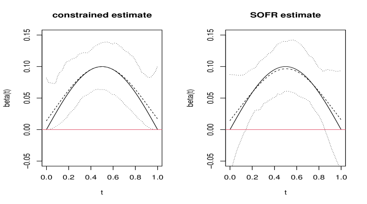
Figure 1: Estimated coefficient function (dashed line) and true coefficient function (solid line) along with $95\%$ point-wise confidence interval (dotted lines) from the constrained (left) and unconstrained (right) method, simulation scenario A, n=50.

Sample size (n)	Constrained method	Unconstrained method	P-value
25	0.9 (1.0)	1.3 (1.1)	2.99$\times 10^{-5}$
50	0.4 (0.3)	0.6 (0.4)	1.5$\times 10^{-6}$
100	0.2 (0.2)	0.3 (0.2)	0.0004

Table 1: Average integrated mean square error ($\times$ 1000) over 200 Monte-Carlo replications, scenario A. Standard errors of IMSE ($\times$ 1000) are reported in the parenthesis. P-values are obtained from two sample t-test.

Projection-based confidence intervals

We apply the projection based method outlined in Algorithm 1 to obtain point-wise asymptotic $95\%$ confidence interval of the regression coefficient function $\beta(t)$ under the shape constraint $\beta(t)>0$. Table S1 in Supplementary Material reports the average empirical coverage of the confidence intervals across the three sample sizes for a range of choices for the order of the Bernstein polynomial basis, $N$. Average estimated coverages are close to the nominal $95\%$ coverage for $N\geq 4$, which is the average order of the Bernstein polynomial basis chosen by our proposed cross-validation criterion. The average width of the confidence interval is found to be comparable or smaller than the unconstrained ("pfr") method for choices of $N$ around $N_{0}=4$. The projection based confidence interval for a particular replication ($n=100$) is displayed in Figure S1 in Supplementary Material.

Testing shape constraints

We consider testing the following shape constraints for the simulation scenario A. i) $H_{0}:\beta_{1}(t)\geq 0\hbox{ for all $t\in[0,1]$}$, ii) $H_{0}:\beta_{1}(t)\hskip 5.69054pt\textit{is concave}\hbox{ for all $t\in[0,1]$}$ iii) $H_{0}:\beta_{1}(t)\hskip 5.69054pt\textit{is increasing}$ for all $t\in[0,1]$. The true coefficient function in this scenario is $\beta(t)=0.1*sin(\pi t)$ which satisfy i) and ii) but does not satisfy iii). Table 2 displays the rejection rates of the bootstrap test for the three null hypothesis and three sets of sample sizes for the nominal level of $\alpha=0.05$.

$H_{0}$	$n=25$	$n=50$	$n=100$
$\beta_{1}(t)\geq 0$	0.055	0.05	0.065
$\beta_{1}(t)\hskip 5.69054pt\textit{is concave}$	0.04	0.07	0.055
$\beta_{1}(t)\hskip 5.69054pt\textit{is increasing}$	0.235	0.55	0.84

Table 2: Rejection rates for the respective hypothesis from the bootstrap based test based on 200 M.C simulations from Scenario A.

We notice the rejection rates remain close to the nominal level of $0.05$ when the null hypothesis is true (case i and ii) and is increasing to 1 as the sample size increase when the null is false (case iii) indicating consistency of the proposed testing method.

Performance under scenario B:

We consider estimation in the functional linear concurrent model of scenario B under the constraint $\beta_{1}(t)$ is decreasing. The average order of Bernstein-polynomial basis chosen by five-fold ($V=5$) cross-validation was $N=5$, across the three sample sizes. Figure 2 displays the estimated coefficient function $\beta_{1}(t)$ (for sample size $n=50$) averaged over 200 M.C replications from both the constrained and unconstrained approach (smoothing spline implemented using "pffr" function within the refund package) along with their $95\%$ point-wise confidence intervals based on the Monte-Carlo replications.

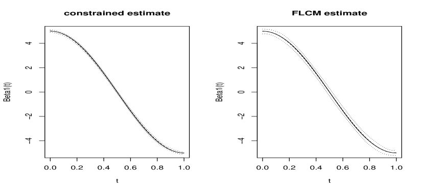
Figure 2: Estimated coefficient function (dashed line) and true coefficient function (solid line) along with $95\%$ point-wise confidence interval (dotted lines) from the constrained (left) and unconstrained (right) method, simulation scenario B, n=50.

It can be noticed the constrained approach produce much narrower confidence interval of the estimate indicating lower uncertainty of the estimated function in the restricted parameter space. The M.C average mean square error (IMSE) (multiplied by 100) of the estimated coefficient function $\hat{\beta}_{1}(t)$ from the constrained and unconstrained method is reported in Table 3. It can be observed that the proposed constrained estimates have much smaller average IMSE compared to the unconstrained estimates. Across the sample sizes, the constrained estimates are found to be $346\%$ more efficient compared to the unconstrained estimators. As the sample size increase, the IMSE from both the methods again become negligible indicating consistency of the estimators. The IMSE (multiplied by 100) of the estimated coefficient function $\hat{\beta}_{1}(t)$ from the sparse design setup is reported in Table S3 of the Supplementary Material, where similar improvement in efficiency can be noticed from the constrained approach.

Sample size (n)	Constrained method	Unconstrained method	P-value
25	1.23 (1.14)	5.37 (5.15)	$<2.2\times 10^{-16}$
50	0.46 (0.30)	2.13 (1.56)	$<2.2\times 10^{-16}$
100	0.26 (0.15)	1.14 (0.85)	$<2.2\times 10^{-16}$

Table 3: Average integrated mean square error ($\times$ 100) over 200 Monte-Carlo replications, scenario B. Standard errors of IMSE ($\times$ 100) are reported in the parenthesis. P-values are obtained from two sample t-test.

Projection-based confidence intervals

We display the projection-based point-wise asymptotic $95\%$ confidence interval of the regression coefficient function $\beta_{1}(t)$ under the shape constraint: $\beta_{1}(t)$ is decreasing. Table S2 in Supplementary Material reports the average empirical coverage of the confidence intervals across the three sample sizes for a range of choices of $N$. The estimated coverage is close to the nominal $95\%$ coverage for $N\geq 5$, which is the average order of the Bernstein polynomial basis chosen by our proposed cross-validation criterion. The average width of the confidence interval is found to be smaller than the unconstrained ("pffr") method for choices of $N$ around $N_{0}=5$, while yielding the correct coverage. The projection-based confidence interval of $\beta_{1}(t)$ for a particular replication ($n=100$) is displayed in the Supplementary Figure S2.

Testing shape constraints

In this scenario, We test the following shape constraints. i) $H_{0}:\beta_{1}(t)\hskip 5.69054pt\textit{is decreasing}$ $\forall$ $t\in[0,1]$, ii) $H_{0}:\beta_{1}(t)\hskip 5.69054pt\textit{is convex}\hbox{ $\forall$ $t\in[0,1]$}$ iii) $H_{0}:\beta_{1}(t)\hskip 5.69054pt\textit{is concave}$ $\forall$ $t\in[0,1]$. The true coefficient function in this scenario is $\beta_{1}(t)=5cos(\pi t)$ which satisfies i) but does not satisfy ii) and ii). Table 4 displays the rejection rates of the bootstrap test for the three null hypothesis and three sets of sample sizes for the nominal level of $\alpha=0.05$.

$H_{0}$	$n=25$	$n=50$	$n=100$
$\beta_{1}(t)\hskip 5.69054pt\textit{is decreasing}$	0.06	0.07	0.065
$\beta_{1}(t)\hskip 5.69054pt\textit{is convex}$	1	1	1
$\beta_{1}(t)\hskip 5.69054pt\textit{is concave}$	1	1	1

Table 4: Rejection rates for the respective hypothesis from the bootstrap based test based on 200 M.C simulations from Scenario B.

We again observe that the rejection rates remain close to the nominal level of $0.05$ when the null hypothesis is true (case i) and is 1 for all the sample sizes when the null is false (case ii and iii) indicating satisfactory power of the proposed testing method.

Remark 4:
Supplementary Simulation Scenario S1 illustrates that the proposed estimation approach and the projection based asymptotic confidence interval is able to capture the true coefficient function accurately, even when it lies on the boundary of the parameter space (e.g., constant function under decreasing constraint).

Performance under scenario C:

We consider estimation in the FLCM described in simulation scenario C under the constraints $\beta_{1}(t)$ is increasing and $\beta_{1}(t)$ is concave. The average order of Bernstein-polynomial basis chosen by five-fold ($V=5$) cross-validation was $N=5$ across the three sample sizes. Figure 3 displays the estimated coefficient function $\beta_{1}(t)$ averaged over 200 M.C replications from both the constrained and unconstrained approach along with their $95\%$ point-wise confidence intervals.

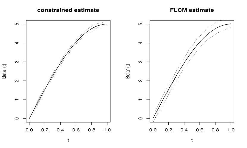
Figure 3: Estimated coefficient function (dashed line) and true coefficient function (solid line) along with $95\%$ confidence interval (dotted lines) from the constrained (left) and unconstrained (right) method, simulation scenario C, n=50.

It can again be noticed the constrained approach produce much narrower confidence interval of the estimated coefficient function $\hat{\beta}_{1}(t)$ indicating lower uncertainty of the estimate in the restricted parameter space. The average M.C mean square error (IMSE) of the estimated coefficient function $\hat{\beta}_{1}(t)$ from both the constrained and unconstrained method is reported in Table 5.

Sample size (n)	Constrained method	Unconstrained method	P-value
25	9.5 (9.8)	49.3 (49.7)	$<2.2\times 10^{-16}$
50	3.1 (2.6)	19.5 (15.1)	$<2.2\times 10^{-16}$
100	1.4 (1.1)	10.5 (8.2)	$<2.2\times 10^{-16}$

Table 5: Average integrated mean square error ($\times$ 1000) over 200 Monte-Carlo replications, scenario C. Standard errors of IMSE ($\times$ 1000) are reported in the parenthesis. P-values are obtained from two sample t-test.

We again observe that the proposed constrained estimates have much smaller average IMSE compared to the unconstrained estimates. Specifically, the constrained estimates are found to be $485\%$ more efficient compared to the unconstrained estimator. As the sample size increase, the IMSE from both the methods again become asymptotically negligible.

The simulation results in this section illustrate the advantages of the proposed estimation method in functional regression models under shape restrictions. For smaller sample sizes, such shape restrictions lead to reduced uncertainty of the coefficient functions in the restricted parameter space.

4 Real Data Applications

In this section, we demonstrate applications of the proposed shape constraint estimation method in functional regression models. First, we consider a mental health schizophrenia collaborative study analyzing evolution of drug effect on the severity of illness. Next, we apply the proposed estimation method for distributional analysis of quantile-functions of physical activity data from Baltimore Longitudinal Study of Aging (BLSA).

4.1 Application 1: Mental Health Schizophrenia Collaborative Study

We consider data from the National Institute of Mental Health Schizophrenia Collaborative Study used in Ahkim et al. (2017). The response of interest is severity of illness measured in the Inpatient Multidimensional Psychiatric Scale (IMPS), ranging from 1 (normal) to 7 (among the most extremely ill). The patients ($n=437$) considered in this study were randomly assigned to a treatment (drug) or placebo and measured at weeks $0,1,2,\ldots,6$. Majority of the patients were measure at weeks $0,1,3,6$ with a few being additionally measured on weeks $2,4,5$. The primary interest here is to assess the efficacy of the drug. We consider a function-on-scalar regression model,

$$Y_{i}(t)=\beta_{0}(t)+G_{i}\beta_{1}(t)+\epsilon_{i}(t),$$ (14)

where $Y_{i}(t)$ denotes disease severity at week $t$ for subject $i$ and $G_{i}$ is a indicator of the treatment group for the subject ($G_{i}=1$, if subject $i$ received drug).

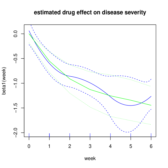
Figure 4: Estimated effect of drug on disease severity as function of week. Constrained ($\beta_{1}(t)\leq 0$) estimate (green solid line) and unconstrained estimate (blue solid line), along with their $95\%$ confidence intervals (dotted for constrained and dashed for unconstrained).

The time-varying coefficient function $\beta_{1}(t)$ captures the effect of the drug on disease severity. A negative $\beta_{1}(t)$ would prove the effectiveness of the drug while a negative and decreasing $\beta_{1}(t)$ would suggest the magnitude of the effectiveness of the drug increase as the weeks progress.

We apply the proposed residual bootstrap-based test in Section 2, and test the constraints i) $\beta_{1}(t)\leq 0$ and ii) $\beta_{1}^{{}^{\prime}}(t)\leq 0$, i.e., $\beta_{1}(t)$ is decreasing. The P-values of the tests are calculated to be 0.53, 0.6 respectively. Hence we fail to reject the hypothesis that the effect of the drug is negative and the effect is decreasing, which matches with the findings by Ahkim et al. (2017). Next, we apply the proposed estimation method in this article under the shape constraint $\beta_{1}(t)\leq 0$, with the prior knowledge that the drug is effective (Ahkim et al., 2017) (ascertained by our proposed test). The degree of the Bernstein polynomial used to model the coefficient functions was chosen to be $3$ by five-fold cross-validation indicating sufficiency of a cubic fit. The estimated coefficient function $\beta_{1}(t)$ capturing the effect of the drug on disease severity is shown in Figure 4. The estimated coefficient function from an unconstrained fit using penalized function-on-scalar regression (obtained using "pffr" function within the refund package in R) is also displayed. The estimates are accompanied with their respective $95\%$ confidence intervals. The average width of the confidence intervals from the constrained method ($0.62$) is found to be smaller compared to that of the unconstrained method ($0.65$).

We notice a negative and mostly decreasing $\beta_{1}(t)$, illustrating the effectiveness of the drug which is captured by both the constrained and the unconstrained estimator.

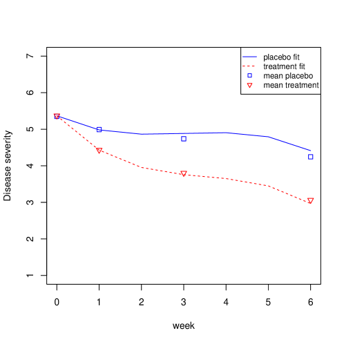
Figure 5: Fitted disease severity trajectories for placebo (solid line) and treatment group (solid line), Schizophrenia data.

The fitted disease severity trajectories from the constrained method is shown in Figure 5 for the treatment and the placebo group, which are very close to the average observed values of disease severity (IMPS).

4.2 Quantile Function on Scalar Regression (QFOSR) of Physical Activity Data from BLSA

As our second example, we model subject-specific distributions of accelerometry-measured physical activity from Baltimore Longitudinal Study of Aging (BLSA), the longest-running scientific study of aging in the United States. Specifically, we are interested in how the subject-specific quantile functions of minute-level activity counts are associated with age, gender, height and weight. We use a quantile function-on-scalar regression framework introduced in Yang et al. (2020) for distributional analysis of physical activity. Prior studies on BLSA (Xiao et al., 2015) have focused on modeling diurnal variability of physical activity. Activity counts were measured using a chest-worn Actiheart physical activity monitor on participants in their free-living environment for several consecutive days. For this analysis, we consider a sample of $n=857$ subjects in BLSA and a single visit of each participant. Table 6 presents the descriptive statistics of the sample.

Characteristic	Complete (n=857)		Male (n=420		Female (n=437)		P value
	Mean	SD	Mean	SD	Mean/Freq	SD
Age	66.83	13.17	68.11	13.36	65.6	12.88	0.005
Height (m)	1.69	0.09	1.76	0.07	1.63	0.06	$<2.2\times 10^{-16}$
Weight (Kg)	78.33	16.37	85.02	14.92	71.90	15.09	$<2.2\times 10^{-16}$

Table 6: Summary statistics for the complete, male and female samples considered for the BLSA analysis.

Subject-specific daily PA is represented via 1440 minute-level activity counts. For the analysis in this paper, we limit our attention to data collected on Mondays for each subject visit. We also only consider activity counts from participants in their most active 10 hour period ($M_{10}^{i}$) (Witting et al., 1990), since this can serve as a proxy period for most of daily physical activity. The activity counts are log transformed using the transformation $A\longrightarrow log(A+1)$ to remove possible skewness in the data. Subsequently, we encode subject level physical activity data in the window $M_{10}^{i}$ (depends on the subject $i$) using subject-specific quantile functions $Q_{i}(p)$ for $i=1,2,\ldots,n=857$, and $p\in[0,1]$. Figure 6 displays the observed (empirical) subject-specific quantile functions $Q_{i}(p)$.

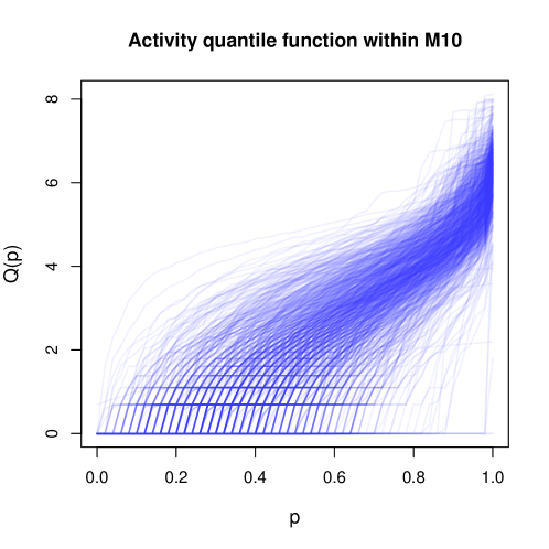
Figure 6: Subject-specific quantile functions of log-transformed physical activity in their most active 10 hour window $M_{10}^{i}$.

We model the subject-day specific quantile functions as outcomes using the quantile function-on-scalar regression model as follows:

$$Q_{i}(p)=\beta_{0}(p)+x_{age,i}\beta_{age}(p)+x_{sex,i}\beta_{sex}(p)+x_{height,i}\beta_{H}(p)+x_{weight,i}\beta_{W}(p)+\epsilon_{i}(p).$$ (15)

The functional regression coefficients $\beta_{age}(p)$, $\beta_{sex}(p)$, $\beta_{H}(p)$ and $\beta_{W}(p)$ capture the effects of age, sex (Male = 1, Female = 0), height, and weight on the quantile level $p$ of subject-specific physical activity. The intercept function $\beta_{0}(p)$ represents the baseline $p-th$ quantile level of physical activity. Yang et al. (2020) proposed to use quantlets, data-driven basis functions, for estimating the functional regression coefficients in QFOSR. The quantlet based estimation approach does not explicitly impose monotonicity in the predicted quantile functions, although the observed (empirical) quantile functions are monotone (Yang et al., 2020), and most of the predicted quantile functions in their applications were found to be monotone and non-decreasing.

Yang (2020) proposed a non-decreasing basis based estimation using I-splines (Ramsay, 1988) or Beta CDFs which enforce this monotonicity at the estimation step. This produces the coefficient functions of form $\beta_{a}(p)=\sum_{k=1}^{K}\Psi_{k}(p)\hat{\beta}_{ak}$, where $\hat{\beta}_{ak}\geq 0$. Notice that this essentially enforces the coefficient functions of the scalar predictors to be monotone and non-decreasing which might not be necessarily true for many of the covariates.

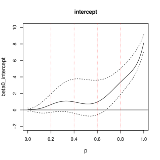
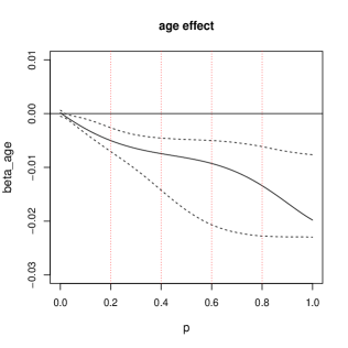
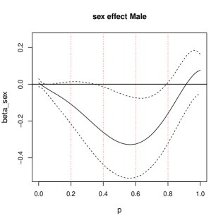
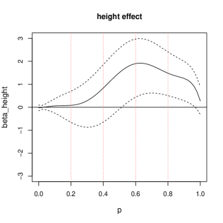
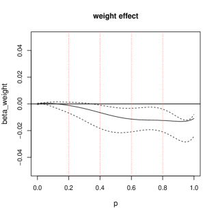
Figure 7: Estimated quantile level effect of scalar (age, sex, height, weight) predictors on quantile function of physical activity in BLSA data using the quantile function-on-scalar regression model (13). Constrained BP estimates ($\beta_{age}(p)$ is decreasing) are shown in solid lines, along with their projection based $95\%$ confidence intervals (shown in dotted lines).

We start with fitting unconstrained regression model (15) which is shown in Figure S4. Several of the functional coefficients (e.g., age, gender etc.) are not necessarily non-decreasing. The age functional coefficient, in particular, appears to be decreasing, indicating an accelerated decrease in maximal levels of PA with increasing age (Varma et al., 2017). To further confirm this phenomenon, we test the null hypothesis $H_{0}:\beta_{age}(p)\hskip 5.69054pt\textit{is decreasing}\hbox{ for all $p\in[0,1]$}$ using the proposed bootstrap test ($B=200$) in this article. The p-value of the test is calculated to be $0.12$, hence we fail to reject the null hypothesis that $\beta_{age}(p)$ is decreasing.

Therefore, next, we impose the monotonicity constraint that $\beta_{age}(p)$ is decreasing. We assume a common degree of smoothness (due to computational tractability) in the coefficient functions which is controlled by the order the Bernstein polynomial basis $N$. The common order of the Bernstein polynomial basis used to model all regression coefficient functions is chosen to be $7$ using the five-fold cross-validation method.

Figure 7 displays the estimated coefficient functions from the proposed Bernstein based constrained estimation approach along with their point-wise asymptotic $95\%$ confidence intervals constructed using the projection method. The estimated effect of age $\hat{\beta}_{age}(p)$ is found to be negative and decreasing over $p$ illustrating that physical activity not only decrease with age (Xiao et al., 2015; Varma et al., 2017), but maximal levels of physical activity are decreasing with a faster rate. Based on the confidence intervals, the effect of age on PA is significant across all quantile levels.

The estimated effect of gender (Male) $\hat{\beta}_{sex}(p)$ indicates that males have higher maximal capacity of physical activity (for $p>0.8$) while females have higher activity levels in the range of $p$ between $0$ and $0.8$. In particular, females are shown to have significantly higher moderate levels of PA ($p\in(0.4,0.8)$) which is consistent with the findings of Xiao et al. (2015). For height, we see a significant positive effect $\hat{\beta}_{height}(p)$, especially, across a mid-range of $p$. The estimated effect $\hat{\beta}_{weight}(p)$ is negative and appears to be decreasing, indicating an accelerated decrease of maximal levels of PA due to the increased weight.

Fitted quantile functions stratified by gender are shown in Figure 8 across different ages and the centered values of height and weight. Similarly, the predicted physical activity quantile function as function of weight is also displayed in Figure 8. We notice the predicted quantile functions to be non decreasing and a clear separation among them with respect to age and weight. These results offer important scientific insights and a deeper understanding of dependence between subject-specific physical activity and demographic factors.

Remark 5:
Our analysis in this section illustrates that not all functional regression coefficients (e.g., age) are non-decreasing in QFOSR. In Appendix D of Supplementary Material, we illustrate a method outlining a sufficient condition for the monotonicity of the quantile function which makes much weaker assumption compared to Yang (2020), allowing for a more flexible modeling of functional regression coefficients in QFOSR. We leave this as a future work to be explored more deeply.

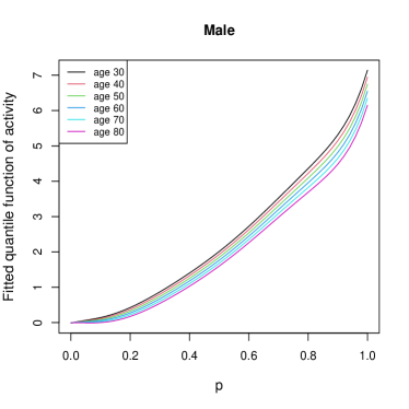
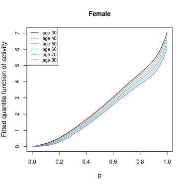
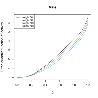
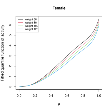
Figure 8: Predicted quantile functions of physical activity for Male and Female for different ages at mean values of height and weight (top) and the predicted quantile function of physical activity for Male and Female for different weights at mean values of age and height (bottom).

5 Discussion

We have developed a new estimation method for dealing with shape-constrained functional regression coefficients in common functional regression models. The estimation approach extends the one of (Wang and Ghosh, 2012). It is shown that the key problem of shape restricted estimation is reduced to a linear inequality constrained least squares problem, where the constraint matrices are universal and do not depend on the value of the basis functions, the observed time-points, or the order of the splines unlike the B-spline based constrained estimation approaches (Ahkim et al., 2017).

The proposed approach is computationally efficient and can be implemented with existing methods of quadratic programming. The constrained estimator is shown to be a projection of the unconstrained estimator, and consistency of the constrained estimator is established under the same regularity conditions as the unconstrained estimator. Projection-based point-wise asymptotic confidence intervals are developed for the constrained functional regression coefficients providing uncertainty quantification of the estimates. A residual bootstrap-based test is proposed that is based on the constrained estimation method. This further facilitates testing of various shape constraints in considered functional regression problems. Our empirical analysis illustrates that the proposed constrained estimation method can lead to reduced uncertainty of the functional coefficient in the restricted parameter space.

Applications shown on schizophrenia collaborative study and Baltimore Longitudinal Study of Aging illustrate the use of the proposed estimation method under prior constraints and offer important scientific insights into these problems. Although the estimation method is illustrated for functional data observed on a dense and regular grid, the method can be extended to more general scenarios where functional data are observed on irregular and sparse domains and covariates observed with measurement error. In such sparse setups, although, the individual number of observations $m_{i}$ can be small, and $\bigcup_{i=1}^{n}\bigcup_{j=1}^{m_{i}}{t_{ij}}$ has to be dense in $\mathcal{T}$. Functional principal component analysis (FPCA) could be applied to de-noise the functional covariates and get their predicted trajectories at all time-points of interest (Ghosal et al., 2020). The proposed estimation method for both functional and scalar response can then be used under the above scenarios. Examples include the schizophrenia collaborative study and the additional simulation set up under Scenario B of this article.

There are many research problems that remain to be explored based on this current work. One of the limitations of the current approach is the absence of a theoretically optimal choice for the order of the Bernstein polynomial basis $N$. Currently it is chosen in a data driven way and it has shown a satisfactory performance in our empirical results. We have considered three common functional regression models (SOFR, FOSR, FOFR) and shown the application of the proposed estimation method under shape constraints. The models illustrated in this article are building blocks of functional regression models (Ramsay and Silverman, 2005) and are limited in assuming linear effects of the predictors on the response, where as in many real world applications the effects might as well be nonlinear. Multiple extensions have been proposed in scalar-on-function (Reiss et al., 2010), function-on-scalar and function-on-function regression models (Kim et al., 2018) modeling dependence between scalar/functional response and scalar/functional covariates via unknown nonparametric functions. It would be of interest to explore the proposed Bernstein polynomial based estimation approach to extend to these models under prior shape constraints on the nonparametric functions.

Another interesting area of work would be to extend the proposed estimation method beyond continuous response and allow scalar/functional responses coming from a general exponential family, e.g, binary data, count data etc. Using the proposed Bernstein polynomial based approach, in such cases would lead to optimizing a negative log-likelihood criterion under linear inequality constraints. One natural idea would be to use a second order Taylor approximation (James et al., 2020) of the log likelihood around the current estimate and solve iteratively a least square objective function under the linear inequality constraints. A Bayesian framework for generalized linear model could also be adapted to incorporate the prior restrictions (Ghosal and Ghosh, 2022). Extending the proposed shape constrained estimation method to such general classes of functional regression models would allow more diverse applications and remain areas for future research.

Software

Software implementation via R (R Core Team, 2018) and illustration of the proposed framework is available online with this article.

Supplementary Material

Additional methodological illustrations and Supplementary Tables and Figures are available online with the Supplementary Material.

References

- Ahkim et al. (2017) Ahkim, M., I. Gijbels, and A. Verhasselt (2017). Shape testing in varying coefficient models. Test 26(2), 429–450.
- Birke and Dette (2007) Birke, M. and H. Dette (2007). Estimating a convex function in nonparametric regression. Scandinavian Journal of Statistics 34(2), 384–404.
- Carnicer and Pena (1993) Carnicer, J. M. and J. M. Pena (1993). Shape preserving representations and optimality of the bernstein basis. Advances in Computational Mathematics 1(2), 173–196.
- Chang et al. (2005) Chang, I.-S., C. A. Hsiung, Y.-J. Wu, and C.-C. Yang (2005). Bayesian survival analysis using bernstein polynomials. Scandinavian journal of statistics 32(3), 447–466.
- Chen et al. (2016) Chen, Y., J. Goldsmith, and R. T. Ogden (2016). Variable selection in function-on-scalar regression. Stat 5(1), 88–101.
- Davidson and Flachaire (2008) Davidson, R. and E. Flachaire (2008). The wild bootstrap, tamed at last. Journal of Econometrics 146(1), 162–169.
- Dette et al. (2006) Dette, H., N. Neumeyer, and K. F. Pilz (2006). A simple nonparametric estimator of a strictly monotone regression function. Bernoulli 12(3), 469–490.
- Eilers et al. (2009) Eilers, P. H., B. Li, and B. D. Marx (2009). Multivariate calibration with single-index signal regression. Chemometrics and Intelligent Laboratory Systems 96(2), 196–202.
- Fan et al. (2015) Fan, Y., G. M. James, and P. Radchenko (2015). Functional additive regression. The Annals of Statistics 43(5), 2296–2325.
- Fan and Reimherr (2017) Fan, Z. and M. Reimherr (2017). High-dimensional adaptive function-on-scalar regression. Econometrics and statistics 1, 167–183.
- Farouki and Goodman (1996) Farouki, R. and T. Goodman (1996). On the optimal stability of the bernstein basis. Mathematics of computation 65(216), 1553–1566.
- Freyberger and Reeves (2018) Freyberger, J. and B. Reeves (2018). Inference under shape restrictions. Available at SSRN 3011474.
- Ghosal and Ghosh (2022) Ghosal, R. and S. K. Ghosh (2022). Bayesian inference for generalized linear model with linear inequality constraints. Computational Statistics & Data Analysis 166, 107335.
- Ghosal and Maity (2021) Ghosal, R. and A. Maity (2021). Variable selection in nonlinear function-on-scalar regression. Biometrics.
- Ghosal et al. (2020) Ghosal, R., A. Maity, T. Clark, and S. B. Longo (2020). Variable selection in functional linear concurrent regression. Journal of the Royal Statistical Society: Series C (Applied Statistics) 69(3), 565–587.
- Ghosal and Saha (2021) Ghosal, R. and E. Saha (2021). Impact of the covid-19 induced lockdown measures on pm2. 5 concentration in usa. Atmospheric Environment 254, 118388.
- Goldfarb and Idnani (1982) Goldfarb, D. and A. Idnani (1982). Dual and primal-dual methods for solving strictly convex quadratic programs. In Numerical analysis, pp. 226–239. Springer.
- Goldfarb and Idnani (1983) Goldfarb, D. and A. Idnani (1983). A numerically stable dual method for solving strictly convex quadratic programs. Mathematical programming 27(1), 1–33.
- Goldsmith et al. (2016) Goldsmith, J., X. Liu, J. Jacobson, and A. Rundle (2016). New insights into activity patterns in children, found using functional data analyses. Medicine and science in sports and exercise 48(9), 1723.
- Grenander (1981) Grenander, U. (1981). Abstract inference. Technical report.
- Hall and Huang (2001) Hall, P. and L.-S. Huang (2001). Nonparametric kernel regression subject to monotonicity constraints. Annals of Statistics 29(3), 624–647.
- Hastie and Tibshirani (1993) Hastie, T. and R. Tibshirani (1993). Varying-coefficient models. Journal of the Royal Statistical Society. Series B (Methodological) 55, 757–796.
- Hoover et al. (1998) Hoover, D. R., J. A. Rice, C. O. Wu, and L.-P. Yang (1998). Nonparametric smoothing estimates of time-varying coefficient models with longitudinal data. Biometrika 85(4), 809–822.
- Hu et al. (2009) Hu, Y., X. He, J. Tao, and N. Shi (2009). Modeling and prediction of children’s growth data via functional principal component analysis. Science in China Series A: Mathematics 52(6), 1342–1350.
- Huang et al. (2004) Huang, J. Z., C. O. Wu, and L. Zhou (2004). Polynomial spline estimation and inference for varying coefficient models with longitudinal data. Statistica Sinica 14, 763–788.
- James et al. (2020) James, G. M., C. Paulson, and P. Rusmevichientong (2020). Penalized and constrained optimization: An application to high-dimensional website advertising. Journal of the American Statistical Association 115(530), 538–554.
- Kim et al. (2018) Kim, J., A. Maity, and A.-M. Staicu (2018). Additive nonlinear functional concurrent model. Statistics and Its Interface 11, 669–685.
- Kim et al. (2018) Kim, J. S., A.-M. Staicu, A. Maity, R. J. Carroll, and D. Ruppert (2018). Additive function-on-function regression. Journal of Computational and Graphical Statistics 27(1), 234–244.
- Kim (2006) Kim, M.-O. (2006). Quantile regression with shape-constrained varying coefficients. Sankhyā: The Indian Journal of Statistics 68(3), 369–391.
- Kowal and Bourgeois (2020) Kowal, D. R. and D. C. Bourgeois (2020). Bayesian function-on-scalars regression for high-dimensional data. Journal of Computational and Graphical Statistics 29(3), 629–638.
- Lim and Glynn (2012) Lim, E. and P. W. Glynn (2012). Consistency of multidimensional convex regression. Operations Research 60(1), 196–208.
- Lorentz (2013) Lorentz, G. G. (2013). Bernstein polynomials. American Mathematical Soc.
- McKay Curtis and Ghosh (2011) McKay Curtis, S. and S. K. Ghosh (2011). A variable selection approach to monotonic regression with bernstein polynomials. Journal of Applied Statistics 38(5), 961–976.
- McLean et al. (2014) McLean, M. W., G. Hooker, A.-M. Staicu, F. Scheipl, and D. Ruppert (2014). Functional generalized additive models. Journal of Computational and Graphical Statistics 23(1), 249–269.
- Meyer (2008) Meyer, M. C. (2008). Inference using shape-restricted regression splines. Annals of Applied Statistics 2(3), 1013–1033.
- Meyer (2018) Meyer, M. C. (2018). A framework for estimation and inference in generalized additive models with shape and order restrictions. Statistical Science 33(4), 595–614.
- Pya and Wood (2015) Pya, N. and S. N. Wood (2015). Shape constrained additive models. Statistics and computing 25(3), 543–559.
- R Core Team (2018) R Core Team (2018). R: A Language and Environment for Statistical Computing. Vienna, Austria: R Foundation for Statistical Computing.
- Ramsay and Silverman (2005) Ramsay, J. and B. Silverman (2005). Functional Data Analysis. New York: Springer-Verlag.
- Ramsay (1988) Ramsay, J. O. (1988). Monotone regression splines in action. Statistical science 3(4), 425–441.
- Reiss et al. (2017) Reiss, P. T., J. Goldsmith, H. L. Shang, and R. T. Ogden (2017). Methods for scalar-on-function regression. International Statistical Review 85(2), 228–249.
- Reiss et al. (2010) Reiss, P. T., L. Huang, and M. Mennes (2010). Fast function-on-scalar regression with penalized basis expansions. The international journal of biostatistics 6(1).
- Scheipl et al. (2015) Scheipl, F., A.-M. Staicu, and S. Greven (2015). Functional additive mixed models. Journal of Computational and Graphical Statistics 24(2), 477–501.
- Turlach et al. (2019) Turlach, B. A., A. Weingessel, and C. Moler (2019). Functions to Solve Quadratic Programming Problems. 1.5-8.
- Vanbrabant and Rosseel (2019) Vanbrabant, L. and Y. Rosseel (2019). Restricted Statistical Estimation and Inference for Linear Models. 0.2-250.
- Varma et al. (2017) Varma, V. R., D. Dey, A. Leroux, J. Di, J. Urbanek, L. Xiao, and V. Zipunnikov (2017). Re-evaluating the effect of age on physical activity over the lifespan. Preventive medicine 101, 102–108.
- Wang and Ghosh (2012) Wang, J. and S. K. Ghosh (2012). Shape restricted nonparametric regression with bernstein polynomials. Computational Statistics & Data Analysis 56(9), 2729–2741.
- Witting et al. (1990) Witting, W., I. Kwa, P. Eikelenboom, M. Mirmiran, and D. F. Swaab (1990). Alterations in the circadian rest-activity rhythm in aging and alzheimer’s disease. Biological psychiatry 27(6), 563–572.
- Wu et al. (2010) Wu, Y., J. Fan, and H.-G. Müller (2010). Varying-coefficient functional linear regression. Bernoulli 16(3), 730–758.
- Xiao et al. (2015) Xiao, L., L. Huang, J. A. Schrack, L. Ferrucci, V. Zipunnikov, and C. M. Crainiceanu (2015). Quantifying the lifetime circadian rhythm of physical activity: a covariate-dependent functional approach. Biostatistics 16(2), 352–367.
- Yagi et al. (2020) Yagi, D., Y. Chen, A. L. Johnson, and T. Kuosmanen (2020). Shape-constrained kernel-weighted least squares: Estimating production functions for chilean manufacturing industries. Journal of Business & Economic Statistics 38(1), 43–54.
- Yang (2020) Yang, H. (2020). Random distributional response model based on spline method. Journal of Statistical Planning and Inference 207, 27–44.
- Yang et al. (2020) Yang, H., V. Baladandayuthapani, A. U. Rao, and J. S. Morris (2020). Quantile function on scalar regression analysis for distributional data. Journal of the American Statistical Association 115(529), 90–106.
- Yao and Müller (2010) Yao, F. and H.-G. Müller (2010). Functional quadratic regression. Biometrika 97(1), 49–64.
- Yao et al. (2005a) Yao, F., H.-G. Müller, and J.-L. Wang (2005a). Functional data analysis for sparse longitudinal data. Journal of the American Statistical Association 100(470), 577–590.
- Yao et al. (2005b) Yao, F., H.-G. Müller, and J.-L. Wang (2005b). Functional linear regression analysis for longitudinal data. The Annals of Statistics 33(6), 2873–2903.