Conditions for Clump Survival in High-z Disc Galaxies

Abstract

We study the survival versus disruption of the giant clumps in high-redshift disc galaxies, short-lived (S) versus long-lived (L) clumps and two L sub-types, via analytic modeling tested against simulations. We develop a criterion for clump survival, with or without their gas, based on a predictive survivability parameter $S$. It compares the energy sources by supernova feedback and gravitational contraction to the clump binding energy and losses by outflows and turbulence dissipation. The clump properties are derived from Toomre instability, approaching virial and Jeans equilibrium, and the supernova energy deposit is based on an up-to-date bubble analysis. For moderate feedback levels, we find that L clumps exist with circular velocities $\sim\!50\,{\rm km}\,{\rm s}^{-1}$ and masses $\!\geq\!\!10^{8}M_{\odot}$. They are likely in galaxies with circular velocities $\!\geq\!\!200\,{\rm km}\,{\rm s}^{-1}$, consistent at $z\!\sim\!2$ with the favored stellar mass for discs, $\!\geq\!\!10^{9.3}M_{\odot}$. L clumps favor disc gas fractions $\!\geq\!\!0.3$, low-mass bulges and redshifts $z\!\sim\!2$. The likelihood of L clumps is reduced if the feedback is more ejective, e.g., if the supernovae are optimally clustered, if radiative feedback is very strong, if the stellar initial mass function is top-heavy, or if the star-formation-rate efficiency is particularly high. A sub-type of L clumps (LS), which lose their gas in several free-fall times but retain bound stellar components, may be explained by a smaller contraction factor and stronger external gravitational effects, where clump mergers increase the SFR efficiency. The more massive L clumps (LL) retain most of their baryons for tens of free-fall times with a roughly constant star-formation rate.

1 Introduction

The typical massive star-forming galaxies at the peak epoch of galaxy formation, in the redshift range $z\!\sim\!1\!-\!3$, are dominated by extended rotating and turbulent gas-rich discs (Genzel et al., 2006; Förster Schreiber et al., 2006; Genzel et al., 2008; Tacconi et al., 2010; Genzel et al., 2011; Tacconi et al., 2013; Genzel et al., 2014; Förster Schreiber et al., 2018), each hosting several giant star-forming clumps (Elmegreen & Elmegreen, 2005; Genzel et al., 2006, 2008; Guo et al., 2012, 2015; Fisher et al., 2017; Guo et al., 2018; Huertas-Company et al., 2020; Ginzburg et al., 2021). Most of these clumps are commonly assumed to form by gravitational disc instability (Toomre, 1964). This process has been simulated both in isolated discs (Noguchi, 1999; Immeli et al., 2004b, a; Bournaud, Elmegreen & Elmegreen, 2007; Genzel et al., 2008) and in a cosmological setting (Dekel, Sari & Ceverino, 2009; Agertz, Teyssier & Moore, 2009; Ceverino, Dekel & Bournaud, 2010; Ceverino et al., 2012), particularly in Mandelker et al. (2014), Mandelker et al. (2017), Ginzburg et al. (2021) and Dekel et al. (2021). Given the high gas fraction in $z\!\sim\!2$ galaxies (e.g., Daddi et al., 2010; Tacconi et al., 2018), the typical clump mass predicted by Toomre instability is on the order of a few percents of the disc mass, which makes the clumps play an important dynamical role in the evolution of these discs, a process dubbed “violent disc instability” (VDI) (e.g., Dekel, Sari & Ceverino, 2009; Dekel & Burkert, 2014). Gas-rich clumps are predicted to form with a mass near and below the characteristic Toomre mass and preferably at relatively large disc radii (see Dekel et al., 2021, for evidence in simulations and observations). Those clumps that survive disruption by stellar and supernova feedback are predicted to migrate toward the disc centre due to VDI-driven torques in a few disc orbital times, corresponding to several hundred Megayears at $z\!\sim\!2$ (e.g., Dekel, Sari & Ceverino, 2009; Ceverino, Dekel & Bournaud, 2010; Krumholz & Burkert, 2010; Cacciato, Dekel & Genel, 2012; Forbes, Krumholz & Burkert, 2012; Forbes et al., 2014; Krumholz et al., 2018; Dekel et al., 2020b).

Simulations reveal that the clumps can be divided into two major types. One consists of long-lived clumps (hereafter L clumps) that remain bound and live for tens of clump free-fall times or more, allowing them enough time to complete their inward migration. The other involves short-lived clumps (hereafter S clumps), which are disrupted after a few free-fall times (Mandelker et al., 2017). Using machine learning, the two types of clumps as identified in the VELA-3 cosmological simulations (§LABEL:sec:sim_type) were also identified in the large catalog of observed clumps from the CANDELS-HST survey Guo et al. (2018), with consistent relative distributions of clump masses, radial positions in the discs and host-galaxy masses (Ginzburg et al., 2021).

According to a wide variety of existing simulations, the clump type depends on certain clump properties at formation, on certain host-galaxy properties, and on the assumed subgrid physical models for star formation and especially feedback. Mandelker et al. (2017), based on the VELA-3 cosmological simulations, found that L clumps tend to form above a threshold mass of $\sim\!10^{8}M_{\odot}$, while S clumps dominate at smaller clump masses. The L clumps were found to be more compact, round and bound, while the S clumps are more diffuse, elongated and they become unbound. In terms of galaxy properties, the L clumps in VELA-3 tend to reside in more massive galaxies, consistent with the predicted mass threshold for long-lived extended discs at a halo mass of $M_{\rm v}\!\sim\!2\times 10^{11}M_{\odot}$ (Dekel et al., 2020a). Based on isolated-galaxy simulations, the clump formation, mass and longevity are correlated with a high gas fraction in the disc (Fensch & Bournaud, 2021; Renaud, Romeo & Agertz, 2021).

Most importantly, the clump type is very sensitive to the subgrid feedback model adopted in the simulation. The VELA-3 simulations, that assume a moderate supernova feedback strength with a modest effective radiative momentum driving of $2\!-\!3L/c$ (where $L$ is the clump luminosity), give rise to clumps of the two types. On the other hand, the VELA-6 simulations (Ceverino et al. in preparation), of the same suite of galaxies but with a stronger feedback, turn out to produce mostly S clumps with a negligible population of L clumps even at the massive end (see below). This recovers the results from simulations that put in very strong winds (Genel et al., 2012), or that include enhanced radiative feedback of $30\!-\!50L/c$ due to strong trapping of infra-red photons and additional elements of feedback (Hopkins, Quataert & Murray, 2012a; Oklopčić et al., 2017). Such simulations produced only S clumps.

On the theory side, Dekel, Sari & Ceverino (2009), based on Dekel & Silk (1986), crudely estimated that supernova feedback by itself may not have enough power to disrupt the massive clumps. Murray, Quataert & Thompson (2010) argued that momentum-driven radiative stellar feedback, enhanced by infra-red photon trapping, could disrupt the clumps on a dynamical timescale, as it does in the local molecular clouds. However, Krumholz & Dekel (2010) pointed out that such an explosive disruption would be possible in the high-redshift giant clumps only if the efficiency of star-formation rate (SFR) in a free-fall time is as high as $\epsilon\!\sim\!0.1$, significantly larger than what is implied by the observed Kennicutt-Schmidt relation in different types of galaxies at different redshifts, namely $\epsilon$ of about one to a few percent (Tacconi et al., 2010; Krumholz, Dekel & McKee, 2012; Freundlich et al., 2013). Dekel & Krumholz (2013) proposed instead that outflows from high-redshift clumps, with mass-loading factors $\eta$ of order unity to a few, are driven by steady momentum-driven outflows from stars over many tens of free-fall times. Their analysis is based on the finding from high-resolution 2D simulations that radiation trapping is negligible because it destabilizes the wind (Krumholz & Thompson, 2012, 2013). Each photon can therefore contribute to the wind momentum only once, so the radiative force is limited to $\sim\!L/c$. Combining radiation, protostellar plus main-sequence winds, and supernovae, Dekel & Krumholz (2013) estimated the total direct injection rate of momentum into the outflow to be $\sim\!2.5L/c$. The adiabatic phase of clustered supernovae and main-sequence winds may double this rate (Gentry et al., 2017). The predicted mass loading factors of order unity were argued in Dekel & Krumholz (2013) to be consistent with the values deduced from the pioneering observations of outflows from giant clumps (Genzel et al., 2011; Newman et al., 2012). They concluded that most massive clumps are expected to complete their migration prior to gas depletion. With the additional gas accretion onto the clumps, they argued that the clumps are actually expected to grow in mass as they migrate inward.

Dekel et al. (2021) studied the evolution of the properties of the massive clumps during their migration through the disc. They developed an idealized analytic “bathtub” model for a single clump, where clump gas turns into stars and the clump exchanges gas and stars with the disc through accretion, feedback-driven outflows and tidal stripping. The clump evolution is governed by the balance between these processes under conservation of gas and stellar mass, which lead to an analytic solution. The model reveals how the clump evolution depends on the assumed efficiency of accretion, star formation and outflows. The model predictions were confronted with simulation results, both of isolated gas-rich galaxies at high resolution and of high-redshift galaxies in their cosmological framework, exploring a variety of feedback strengths at moderate levels. The theoretical predictions were confronted with the CANDELS clump catalog of Guo et al. (2018) at $z\!=\!1.5\!-\!3$, indicating that the observed gradients of clump properties as a function of distance from the disc centre are consistent with the predicted migration of massive clumps and the associated mild evolution of clump properties.

Our goal in this paper is to understand the conditions for clump survival versus disruption by feedback, and thus seek the origin of the different clump types in terms of clump and disc properties as well as feedback strength. We do this first via analytic modeling. For clumps in their early stages of evolution, we define a survivability parameter $S$, the ratio of (a fraction of) the clump mass to the outflowing mass. The value of this quantity below or above unity distinguishes between S and L clumps. This parameter can be derived from basic clump properties based on the energy balance in the clump. We consider the energy sources by supernova feedback and gravitational driving of turbulence, and energy sinks by dissipation of turbulence and outflows, in comparison with the clump gravitational binding energy. In this model, the clump properties are deduced from Toomre marginal instability (as in Dekel, Sari & Ceverino, 2009), with the kinematics of fully collapsed clumps obeying Jeans equilibrium (Ceverino et al., 2012). The input by supernova feedback, inspired by Dekel & Silk (1986), is based on up-to-date studies of bubble evolution as in Dekel et al. (2019), fine-tuned in our ongoing work. The gravitational driving of turbulence is estimated from the gravitational collapse and clump encounters. The analytic model is then confronted with the clumps in the VELA-3 and VELA-6 cosmological simulations.

Beyond the distinction between L and S clumps, we address a new sub-division into two types of L clumps that will be identified in the simulations below. One sub-type, to be termed LL, consists of clumps that keep a relatively high gas fraction for many tens of clump free-fall times. The other sub-type, to be termed LS, is made of clumps that lose most of their gas to outflows in $\lower 2.58333pt\hbox{$\;\buildrel<\over{\sim}\;$}\!10$ free-fall times, but keep long-lived bound stellar components that survive for many tens of free-fall times. Our analytic model provides physical explanations for the basic distinction between S and L clumps as well as for the sub-division into LS and LL clumps.

The paper is organized as follows. In §2 to §7 we present the analytic model, and in §8 and §9 we compare the model to simulations. In §2 we introduce the survivability parameter $S$. In §3 we model the clump binding energy and the energy drains by dissipation of turbulence and outflows. In §4 we model the energy sources by supernova feedback and by gravity. In §5 we introduce a correction for clumps that have not reached virial equilibrium. In §6 we use the model to explain the division to S and L clumps and the sub-division to LS and LL clumps. In §7 we identify the dependence of the clump type on the different properties of the clump and the host disc as well as the feedback strength. Then, In §8 we present the division to clump types in the simulations. Finally, in §9, we confront the model predictions with the simulation results. In §10 we summarize our conclusions and discuss them.

2 Condition for clump survival

2.1 A survivability parameter

We consider a clump of mass $M_{\rm c}(t)$, at time $t$ after its formation, that has lost mass $M_{\rm out}(t)$ to outflows up until that time. For a clump in virial equilibrium, we define a clump survivability parameter $S$ such that a criterion for significant mass loss through outflows by time $t$ is

$$S(t)\equiv\frac{0.5\,M_{\rm c}(t)}{M_{\rm out}(t)}\leq 1\,.$$ (1)

While $M_{\rm out}$ is expected to grow steadily in time, $M_{\rm c}$ may tend to have a rather constant value after the early stages of clump buildup, or decline for clumps that lose a significant fraction of their gas to outflows (Dekel et al., 2021). When $S$ is above unity, the clump has retained most of its mass, while when $S$ is below unity, the clump has lost most of its mass to outflows. Eq. (1) is motivated by noticing that for a clump in virial equilibrium, an instantaneous removal of half its mass (in a free-fall time) makes it unbound with zero energy. We will soften the requirement for virial equilibrium in §5 and generalize the definition of $S$ accordingly in eq. (53).

However, a mass loss with $S\!\leq\!1$ does not necessarily imply a total disruption. If the mass loss is adiabatic, over many free-fall times, part of the system may remain bound. A criterion for destructive instantaneous mass loss is thus $\dot{M}_{\rm out}(t)\,t_{\rm ff}\!\geq\!0.5M_{\rm c}(t)$, where $t_{\rm ff}$ is the clump free-fall time. If we crudely approximate $\dot{M}_{\rm out}(t)\!\sim\!M_{\rm out}(t)/t$, where $t$ is the time since clump formation, the criterion for total disruption becomes

$$\tau S(t)\leq 1\,,$$ (2)

where $\tau\!=\!t/t_{\rm ff}$. Thus, at $\tau\!\sim\!1$, a value of $S\!\leq\!1$ that implies removal of most of the gas also indicates a total disruption, $\tau S\!\leq\!1$, namely an S clump. However, if half the mass is lost only by a later time, $S(\tau)\!\leq\!1$ at $\tau$ well above unity, the mass-loss would be totally destructive (S) only if $\tau S\!\leq\!1$ as well, while a bound (stellar) remnant is expected (LS) if $\tau S\!>\!1$.

The quantities $M_{\rm c}$ and $M_{\rm out}$ that define $S$ in eq. (1) can be measured from simulations, as we do below in one version of our analysis, though the measured $M_{\rm out}$ may be rather uncertain, especially at early times when the clump radius is likely to evolve rapidly.

2.2 The survivability by energy balance

As an alternative, we wish to predict $S$ from theoretical considerations, where we express $M_{\rm c}$ and $M_{\rm out}$ by physical quantities that we can estimate using physical arguments and based on an energy balance.

Assuming a spherical clump of mass $M_{\rm c}$ within radius $R_{\rm c}$, the potential is characterized by a circular velocity $V_{\rm c}^{2}\!=\!GM_{\rm c}/R_{\rm c}$. In virial equilibrium, the total energy of the gas per unit mass is

$$-E_{\rm vir}=-\frac{1}{2}V_{\rm c}^{2}=-\frac{1}{2}\frac{GM_{\rm c}}{R_{\rm c}}\,.$$ (3)

We tentatively assume that $V_{\rm c}$ and the gas mass $M_{\rm g}$ are roughly constant during the early phase of clump evolution, before a significant amount of the gas is ejected. This is motivated by analytic modeling and simulations of clump evolution (Dekel et al., 2021), and it will be tested further in simulations below.

The cumulative energy balance by time $t$, per unit gas mass, can be written as

$$E_{\rm sn}(t)+E_{\rm grav}(t)-E_{\rm dis}(t)=E_{\rm vir}+E_{\rm out}(t)\,,$$ (4)

where all the quantities are positive. Except $E_{\rm vir}$, they are all integrals of their rates over time. Each will be evaluated below as a function of certain basic parameters in terms of $V_{\rm c}$ and $\tau$. The terms on the left-hand side represent sources of energy gain and loss. The term $E_{\rm sn}$ is the energy deposited in the gas by stars and supernovae. The term $E_{\rm grav}$ represents the additional mechanical energy sources largely associated with gravity, such as the gravity associated with the initial collapse of the clump, continuous accretion, mergers, tidal effects and shear, all capable of driving turbulence. The term $E_{\rm dis}$ represents the dissipative losses of the turbulence, cascading down to small scales where it thermalizes and can cool radiatively. The terms on the right-hand side represent the energy required to bring the gas from virial equilibrium to outflow. Here $E_{\rm vir}$ is the energy required for bringing the gas from $-E_{\rm vir}$ to $E\!=\!0$, ready for escape, and $E_{\rm out}$ is the extra kinetic energy carried by the outflow.

Using eq. (4), the survivability parameter $S$ as defined in eq. (1) can be approximated by

$$S\!\simeq\!\frac{f_{\rm g,c}^{-1}\,E_{\rm vir}}{E_{\rm out}}\,,$$ (5)

where $f_{\rm g,c}$ is the gas fraction in the clump, starting somewhat below unity and declining in time. This arises from eq. (3) and the relation of $E_{\rm out}$ to $V_{\rm c}$,

$$E_{\rm out}=\frac{1}{2}\frac{M_{\rm out}}{M_{\rm g}}V_{\rm out}^{2}\simeq\frac{M_{\rm out}}{M_{\rm g}}V_{\rm c}^{2}\,,$$ (6)

where the typical outflow velocity is crudely assumed to be near the escape velocity, $V_{\rm out}^{2}\!\simeq\!2\,V_{\rm c}^{2}$. Thus, $S$ can be expressed as

$$S=\frac{f_{\rm g,c}^{-1}}{S^{\prime-1}-1}\,,\quad S^{\prime}\equiv\frac{E_{\rm vir}}{E_{\rm sn}+E_{\rm grav}-E_{\rm dis}}\,.$$ (7)

We note that the critical value for losing mass by outflows that corresponds to $S\!=\!1$ is $S^{\prime}\!=\!1/(f_{\rm g,c}^{-1}+1)$. This is $S^{\prime}\!\sim\!0.5$ for $f_{\rm g,c}\!\sim\!1$ and $S^{\prime}\!\sim\!f_{\rm g,c}$ for $f_{\rm g,c}\!\ll\!1$, which are valid respectively early and late in the clump evolution.

The cumulative specific energies that enter $S$ in eq. (7) will be evaluated below based on theoretical arguments. They all turn out to be proportional to $E_{\rm vir}\tau$, and can be written as

$$E_{\rm sn}=f_{\rm sn}\,V_{\rm c,50}^{-1}\,E_{\rm vir}\,\tau\,,\quad E_{\rm grav}=f_{\rm grav}\,E_{\rm vir}\,\tau\,,$$ (8)

$$E_{\rm dis}=f_{\rm dis}\,E_{\rm vir}\,\tau\,,\quad E_{\rm out}=f_{\rm out}\,E_{\rm vir}\,\tau\,,$$ (9)

with the $f$ factors functions of basic clump parameters, and where $V_{\rm c,50}\!=\!V_{\rm c}/50\,{\rm km}\,{\rm s}^{-1}$ is the main explicit clump property that enters. The clump $V_{\rm c}$ (and $E_{\rm vir}$) will be predicted assuming Toomre disk instability (Toomre, 1964). The feedback energy $E_{\rm sn}$ will be estimated from the theory of supernova bubbles as a function of the turbulence velocity dispersion $\sigma_{\rm c}$. The dissipative energy loss $E_{\rm dis}$ can also be estimated as a function of $\sigma_{\rm c}$. In turn, $\sigma_{\rm c}$ can be related to $V_{\rm c}$ assuming Jeans equilibrium and the degree of angular-momentum conservation during clump formation. The value of $E_{\rm grav}$ can be crudely evaluated during clump formation and at later times. In the following estimates we learn that $f_{\rm sn}$ is of order unity or larger, $f_{\rm dis}\!\sim\!1$, $f_{\rm grav}$ is of order unity or smaller, and $f_{\rm out}\!\ll\!1$.

Inserting eqs. (8) and (9) in $S^{\prime}$ from eq. (7) we obtain

$$S^{\prime}=\frac{1}{(f_{\rm sn}\,V_{\rm c,50}^{-1}+f_{\rm grav}-f_{\rm dis})\,\tau}\,,$$ (10)

which serves as our operational expression for $S^{\prime}$ and $S$. Interestingly, the key quantity $V_{\rm c}$ enters $S^{\prime}$ only through the first term. The dominant factor in determining the value of $S^{\prime}$ is the supernova feedback represented by the first term in the denominator of eq. (10), as $f_{\rm sn}$ varies with the feedback strength and $V_{\rm c}$ varies between massive and low mass clumps. The time dependence enters via $\tau$ as a multiplicative factor for all the terms in the denominator, as well as through possible time dependencies of each $f$ factor.

According to eq. (7), the time $\tau_{(S\!=\!1)}$ when $S$ equals unity is when $S^{\prime-1}\!=\!1+f_{\rm g,c}^{-1}$, which from eq. (10) is at

$$\tau_{(S\!=\!1)}=\frac{1+f_{\rm g,c}^{-1}}{f_{\rm sn}V_{\rm c,50}^{-1}+f_{\rm grav}-f_{\rm dis}}\,.$$ (11)

If the clump is to lose a significant fraction of its gas, a larger value of $\tau_{(S\!=\!1)}$ indicates a later time for gas loss. Similarly, the time that indicates full disruption, when $\tau S\!=\!1$, is given by

$$\tau_{(\tau S\!=\!1)}=[f_{\rm sn}\,V_{\rm c,50}^{-1}+f_{\rm grav}-f_{\rm dis}-f_{\rm g,c}^{-1}]^{-1}\,.$$ (12)

3 Clump properties & energy drains

In the coming two sections we evaluate the relevant energies and the associated $f$ factors that enter $S^{\prime}$ in eq. (10). In the current section we address the relevant clump properties, using Toomre instability to derive the binding energy and using Jeans equilibrium to relate rotation to dispersion velocity, and evaluate the energy losses by outflows and dissipation. In the following section we evaluate the energy gains by supernovae and gravity.

3.1 Star formation rate and outflow energy

The outflow energy can be expressed as a function of the SFR, $\dot{M}_{\rm sf}$, via the mass-loading factor

$$\eta=\frac{\dot{M}_{\rm out}}{\dot{M}_{\rm sf}}\,.$$ (13)

According to the simulations described below, $\eta$ is expected to be of order unity. Following the standard convention, the SFR can be expressed via the free-fall time in the clump, $t_{\rm ff}$, and the SFR efficiency parameter, $\epsilon$, as

$$\dot{M}_{\rm sf}=\epsilon\,\frac{M_{\rm g}}{t_{\rm ff}}\,.$$ (14)

The clump free-fall time is

$$t_{\rm ff}=\left(\frac{3\,\pi}{32\,G\,\rho}\right)^{1/2}\simeq 5.2\,{\rm Myr}\,n_{2}^{-1/2}f_{\rm g,c}^{1/2}\,,$$ (15)

where $\rho$ is the total density in the clump, $n\!=\!100\,{\rm cm}^{-3}\,n_{2}$ is the corresponding gas number density and $f_{\rm g,c}\!\lower 2.58333pt\hbox{$\;\buildrel<\over{\sim}\;$}\!1$ is the gas fraction in the clump in its early phase. We very crudely assumed here $\rho\!=\!f_{\rm g,c}^{-1}\,m_{\rm p}\,n$. A value of $n\!\sim\!100\,{\rm cm}^{-3}$ is expected if the clump has collapsed in 3D by a factor of a few from a gas density of order $1\,{\rm cm}^{-3}$ in the disc.

The SFR efficiency per free-fall time, $\epsilon$, has to be of order a few percent in order to match the Kennicutt-Schmidt law in different environments and redshifts (e.g., Krumholz, Dekel & McKee, 2012). The effective value of $\epsilon$ as defined for the whole clump mass and free-fall time may be larger if the star formation actually occurs in dense sub-regions within the clump, where the free-fall timescale is shorter. We denote $\epsilon\!=\!0.03\,\epsilon_{.03}$.

Assuming a constant SFR and $M_{\rm g}$, using eqs. (13) and (14) one can write

$$M_{\rm out}=\eta\,\dot{M}_{\rm sf}\,t=0.03\,\epsilon_{.03}\,\eta\,M_{\rm g}\,\tau\,,$$ (16)

and express the outflow energy per unit gas mass from eq. (6) as

$$E_{\rm out}=0.03\,\epsilon_{.03}\,\eta\,\tau\,V_{\rm c}^{2}\,.$$ (17)

Comparing eq. (17) to eq. (3), assuming the fiducial values of $\eta$ and $\epsilon$, we learn that $E_{\rm out}\!\ll\!E_{\rm vir}$ in the first few free-fall times, and they become comparable at $\tau\!\sim\!16$.

3.2 Toomre clump binding energy

In order to evaluate the clump properties that enter $E_{\rm vir}$ in eq. (3), we assume that the disc is in marginal Toomre instability (Toomre, 1964) with $Q\!=\!1$. We assume that the clump mass is $\mu\,M_{\rm T}$, where $M_{\rm T}$ is the Toomre mass corresponding to the fastest growing scale. Following Dekel, Sari & Ceverino (2009), Ceverino, Dekel & Bournaud (2010) and Ceverino et al. (2012), we define a key quantity, the cold mass fraction,

$$\delta\equiv\frac{M_{\rm d}}{M_{\rm tot}}\,.$$ (18)

Here $M_{\rm d}$ is the cold mass in the disk (gas and young stars), and $M_{\rm tot}$ is the total mass encompassed by the sphere of the disc radius $R_{\rm d}$ (including gas, stars and dark matter). Assuming a local power law for the disc rotation curve, $V_{\rm d}(r)\!\propto\!r^{\alpha}$, with a characteristic value $V_{\rm d}$, and a disc radial velocity dispersion $\sigma_{r,{\rm d}}$, a Toomre parameter of $Q\!=\!1$ implies that

$$\delta=\sqrt{2}(1+\alpha)^{1/2}\,\frac{\sigma_{r,{\rm d}}}{V_{\rm d}}\,.$$ (19)

Then, the Toomre proto-clump radius relative to the disc radius is

$$\frac{R_{\rm T}}{R_{\rm d}}=\frac{\pi}{4\,(1+\alpha)}\,\delta\,,$$ (20)

and the Toomre clump mass relative to the disc mass is

$$\frac{M_{\rm T}}{M_{\rm d}}=\left(\frac{R_{\rm T}}{R_{\rm d}}\right)^{2}=0.025\,\delta_{.2}^{2}\,,$$ (21)

where $\delta\!=\!0.2\,\delta_{.2}$, the density in the proto-clump is assumed to be similar to the mean density in the disc, and $\alpha\!=\!0$ is assumed. We thus have

$$M_{\rm c}=\mu M_{\rm T}\quad{\rm and}\quad R_{\rm c,i}\!=\!\mu^{1/2}R_{\rm T}\,,$$ (22)

where $R_{\rm c,i}$ is the initial radius of the proto-clump patch in the disc. The clump mass in terms of the cold-disc mass becomes

$$M_{\rm c}=0.25\times 10^{8}M_{\odot}\,\mu_{.5}\,\delta_{.2}^{2}\,M_{\rm d,9.3}\,,$$ (23)

where $M_{\rm d}=10^{9.3}M_{\odot}\,M_{\rm d,9.3}$.

In order to obtain the clump circular velocity, we assume that the clump has collapsed by a contraction factor $c$ from its initial radius to a final radius $R_{\rm c}$,

$$R_{\rm c,i}=cR_{\rm c}\,.$$ (24)

Then, combining eq. (20) and eq. (24), the clump potential well is characterized by

$$V_{\rm c}^{2}=\frac{G\,M_{\rm c}}{R_{\rm c}}=\frac{\pi}{4\,(1+\alpha)}\,c\,\mu^{1/2}\,\delta^{2}\,V_{\rm d}^{2}\,,$$ (25)

recalling that $V_{\rm d}^{2}\!=\!G(\delta^{-1}M_{\rm d})/R_{\rm d}$. Assuming hereafter a flat rotation curve, $\alpha=0$, we obtain for the characteristic clump circular velocity

$$V_{\rm c}\simeq 50\,{\rm km}\,{\rm s}^{-1}\,c_{3}^{1/2}\,\mu_{.5}^{1/4}\,\delta_{.2}\,V_{{\rm d},200}\,,$$ (26)

where $c\!=\!3\,c_{3}$, $\mu\!=\!0.5\mu_{.5}$, $\delta\!=\!0.2\,\delta_{.2}$, and $V_{\rm d}\!=\!200\,{\rm km}\,{\rm s}^{-1}V_{{\rm d},200}$. This could be inserted in eq. (3) for $E_{\rm vir}$.

The fiducial values of the parameters are crudely justified as follows. A contraction factor of $c\!\sim\!3\!-\!5$ is expected for clump virialization and rotation support (Ceverino et al., 2012). A galactic circular velocity of $V_{\rm d}\!\simeq\!1.5V_{\rm v}\!\simeq\!200\,{\rm km}\,{\rm s}^{-1}$ is expected for a galaxy in a halo of $M_{\rm v}\!\sim\!3\times 10^{11}M_{\odot}$ at $z\!\sim\!2$, based on the virial relation, eq. (62) below. This is above the threshold for long-lived disks at all redshifts (Dekel et al., 2020a). This halo mass implies a stellar mass of $M_{\rm s}\!\sim\!3\times 10^{9}M_{\odot}$ (Behroozi et al., 2019), and a comparable gas mass for $f_{\rm g}\!\simeq\!0.5$ (see §7.1). A value of $\delta\!\sim\!0.2$ can be expected for a gas fraction in the disc of $f_{\rm g}\!\sim\!0.5$, given the contribution of the bulge and the dark matter to $M_{\rm tot}$ in the denominator of $\delta$ (see §7.3). Eq. (26) is in good agreement with the values obtained for clumps in the VELA-3 simulations (Mandelker et al., 2017, Fig. 8), where the typical galaxy masses at $z\!\sim\!2$ are indeed comparable to the fiducial values mentioned above, to be discussed further below.

3.3 Rotation and dispersion: Jeans equilibrium

Certain energy terms in eq. (4) depend on the clump velocity dispersion, $\sigma_{\rm c}$, which characterizes the turbulence in the clumps, and is significantly larger than the speed of sound of $\sim\!10\,{\rm km}\,{\rm s}^{-1}$ at a typical temperature of $\sim\!10^{4}$K. In $\sigma_{\rm c}$ we refer to the one-dimensional component of the velocity dispersion, specifically the radial component. Following Ceverino et al. (2012), assuming that the clump is in Jeans equilibrium, $\sigma_{\rm c}$ can be evaluated from $V_{\rm c}$ and the clump contraction factor $c$, as follows.

Assuming cylindrical symmetry, the Jeans equation in the equatorial plane reads

$$V_{\rm c}^{2}=V_{\rm rot,c}^{2}-\frac{r}{\rho}\frac{\partial(\rho\,\sigma_{\rm c}^{2})}{\partial r}\simeq V_{\rm rot,c}^{2}+2\,\sigma_{\rm c}^{2}\,,$$ (27)

where $V_{\rm rot,c}$ is the rotation velocity in the clump, and $\sigma_{\rm c}$ is the radial velocity dispersion, which is assumed to be constant in the second equality. The factor 2 is for an isothermal-sphere-like density profile, $\rho\!\propto\!r^{-2}$. In practice, simulations show that for entire discs this factor can vary between unity near the effective radius of the gas and 4 at five effective radii, well outside the main body of the disc (Kretschmer et al., 2021), indicating that variations may be expected within the clumps as well. We note that with no rotation, $\sigma_{\rm c}^{2}\!\simeq\!0.5V_{\rm c}^{2}$.

For a disc in marginal Toomre stability with $Q\!=\!1$, and a clump contraction factor $c$, we obtain from eq. (19) to eq. (24) that the clump is related to the disc via

$$V_{\rm c}^{2}=\frac{\pi}{2}\,c\,\mu^{1/2}\,\sigma_{r,{\rm d}}^{2}\,,$$ (28)

independent of $\alpha$. Assuming that angular momentum is conserved during the collapse of the clump, one obtains (as in eq. 19 of Ceverino et al., 2012) a second relation between clump and disc,

$$V_{\rm rot,c}^{2}=\frac{\pi^{2}}{32}\,(1+\alpha)\,\mu\,c^{2}\sigma_{r,{\rm d}}^{2}\,.$$ (29)

Using eqs. (28) and (29), we obtain within the clump

$$V_{\rm rot,c}^{2}=\frac{\pi}{16}\,(1+\alpha)\,c\,\mu^{1/2}\,V_{\rm c}^{2}\simeq 0.2\,c\,\mu^{1/2}\,V_{\rm c}^{2}\,,$$ (30)

where the second equality is for a flat rotation curve, $\alpha\!=\!0$. Note that full rotation support, $V_{\rm rot,c}\!=\!V_{\rm c}$, is obtained for a maximum contraction factor $c\!=\!5\,\mu^{-1/2}$. Inserting eq. (30) in eq. (27) we obtain

$$\frac{\sigma_{\rm c}^{2}}{V_{\rm c}^{2}}\simeq 0.5-0.1\,c\,\mu^{1/2}\equiv 0.5\,f_{\sigma}\,.$$ (31)

The factor $f_{\sigma}$ defined here can range from $f_{\sigma}\!=\!1$ in the case of no rotation to $f_{\sigma}\!=\!0.58$ when angular-momentum is conserved during clump collapse, with the fiducial values $c\!=\!3$ and $\mu\!=\!0.5$. This gives

$$\sigma_{\rm c}\simeq 35\,{\rm km}\,{\rm s}^{-1}\,f_{\sigma}^{1/2}\,V_{\rm c,50}\,.$$ (32)

For $V_{\rm c}\!=\!50\,{\rm km}\,{\rm s}^{-1}$, a value of $\sigma_{\rm c}\!\simeq\!35\,{\rm km}\,{\rm s}^{-1}$ is expected if there is no angular momentum, and $\sigma_{\rm c}\!\simeq\!27\,{\rm km}\,{\rm s}^{-1}$ when angular momentum is conserved, so we denote $\sigma_{\rm c}\!=\!30\,{\rm km}\,{\rm s}^{-1}\,\sigma_{30}$.

3.4 Dissipation of Turbulence

Eq. (31) allows us to express $E_{\rm dis}$, the dissipative loss of the turbulence per unit mass, as a function of $V_{\rm c}$. Assuming that the timescale for turbulence decay is $\gamma\,t_{\rm ff}$, where $\gamma$ is a factor of order unity, the dissipated energy by time $t$ is

$$E_{\rm dis}=\frac{3}{2}\sigma_{\rm c}^{2}\,\gamma^{-1}\,\tau=\frac{3}{4}f_{\sigma}\,\gamma^{-1}\,V_{\rm c}^{2}\,\tau\,,$$ (33)

where the turbulence is assumed to be isotropic with $\sigma_{\rm c}$ the one-dimensional velocity dispersion. The corresponding dimensionless factor in eq. (9) is

$$f_{\rm dis}=1.5\,f_{\sigma}\,\gamma^{-1}\,.$$ (34)

A comparison to eq. (3) indicates that $E_{\rm dis}$ becomes comparable to $E_{\rm vir}$ at $\tau$ of order unity or a few, when $E_{\rm out}$ in eq. (17) is still much smaller.

4 Sources: supernovae and gravity

Complementing the previous section, we evaluate in this section the energy input to the clump gas by supernovae and by gravity.

4.1 Energy deposit by Supernova Feedback

Here, we evaluate $E_{\rm sn}(t)$, the energy per unit mass deposited in the clump gas by supernovae bubbles till time $t$. While the feedback also contains contributions from stellar winds and radiative pressure, we tentatively limit the analysis here to the energy deposited in the ISM by supernovae. The calculation is inspired by Dekel & Silk (1986), following the revised treatment of supernova bubbles in Dekel et al. (2019) and ongoing work (Tziperman, Sarkar, Dekel, in preparation). The energy is evaluated here as the sum of the energies deposited by individual supernova bubbles. We assume a constant SFR during the time relevant for clump evolution, motivated by Dekel et al. (2021). The calculation is simplified by the realization that the relevant time of one or more free-fall times is much larger than the fading time of each bubble, $t_{\rm fade}$, and that overlap of active bubbles younger than $t_{\rm fade}$ is negligible as long as they occur in random positions within the clump. An alternative calculation could address super-bubbles generated by supernovae that are clustered in subclumps, e.g., in the spirit of Gentry et al. (2017) and Dekel et al. (2019).

4.1.1 An individual supernova bubble

According to the standard model for the evolution of a supernova bubble in a uniform medium, the first important stage is the Sedov-Taylor adiabatic phase, during which the shock radius grows as $R\!\propto\!t^{2/5}$ and its velocity slows down as $V\!\propto\!t^{-3/5}$. The end of this stage is commonly defined at the cooling time, $t_{\rm cool}$, when the bubble has lost one third of its initial energy to radiation. For an assumed cooling rate (Dekel et al., 2019, eq. 9), which is a fair approximation for a solar-metallicity gas at temperatures in the range $10^{5-7.3}K$, the cooling time is estimated to be (Dekel et al., 2019, eq. 12)

$$t_{\rm cool}\simeq 3.95\,{\rm kyr}\,n_{2}^{-0.55}e_{51}^{0.22}\,,$$ (35)

where $e_{51}$ is the initial supernova energy in units of $10^{51}\,{\rm erg}$. The shell velocity and radius just prior to the cooling time are $V_{\rm cool}\!\simeq\!340\,{\rm km}\,{\rm s}^{-1}\,n_{2}^{0.13}\,e_{51}^{0.066}$ and $R_{\rm cool}\!\simeq\!3.53\,{\rm pc}\,n_{2}^{-0.42}\,e_{51}^{0.29}$.

The second stage is the snow-plow phase, where a dense shell of cold gas is mainly pushed by the pressure of the enclosed hot central volume. The shell mass increases as it sweeps up the ambient gas, and it slows down as $R\!\propto\!t^{2/7}$ and $V\!\propto\!t^{-5/7}$. The velocity of the shock radius in the snow-plow phase is $V_{\rm s}\!=\!(2/7)\,R_{\rm cool}/t$ (note the discontinuity in the velocity at $t_{\rm cool}$, e.g., Sarkar, Gnat & Sternberg, 2021). In the snow-plow phase, the total energy in the bubble is commonly assumed to decline as $\propto t^{-4/7}$, but we adopt a slightly steeper decline of $\propto t^{-0.7}$, based on more involved theoretical arguments and spherical simulations (Dekel et al., 2019).

The bubble is regarded as faded away at time $t_{\rm fade}$, when its outward velocity becomes comparable to the velocity dispersion outside it, $\sigma_{\rm c}$. The energy is deposited until that time, and soon after the bubble melts into the general clump medium. In analogy to eq. 18 of Dekel et al. (2019), the fading time is evaluated to be

$$t_{\rm fade}=73\,{\rm kyr}\,n_{2}^{-0.37}\,e_{51}^{0.32}\,\sigma_{30}^{-7/5}\,,$$ (36)

where $\sigma_{30}=30\,{\rm km}\,{\rm s}^{-1}\,\sigma_{\rm c}$. This fading time is significantly smaller than the clump free-fall time of $\sim 5\,{\rm Myr}$ (eq. 15), over which the clump evolves. The shell radius at that time is

$$R_{\rm fade}=8.1\,{\rm pc}\,n_{2}^{-0.37}\,e_{51}^{0.32}\,\sigma_{30}^{-2/5}\,,$$ (37)

which is significantly smaller than the clump radius of $\lower 2.58333pt\hbox{$\;\buildrel>\over{\sim}\;$}\!200\,{\rm pc}$. The energy deposited in the medium by a single bubble until $t_{\rm fade}$ is

$$e_{\rm fade}\simeq 8.7\times 10^{49}\,{\rm erg}\,n_{2}^{-0.13}\,e_{51}^{0.93}\,\sigma_{30}^{0.98}\,.$$ (38)

4.1.2 Multiple supernova bubbles

Following Dekel & Silk (1986), we write the total deposited energy by time $t$ as

$$M_{\rm g}\,E_{\rm sn}(t)=\int_{0}^{N(t)}e(t-t_{*})\,dN(t_{*})\,,$$ (39)

where $e(t^{\prime})$ is the energy deposited by a single supernova from its birth to time $t^{\prime}$, and $N(t)$ is the cumulative number of supernovae by time $t$. Assuming a constant SFR during the early phases of the clump lifetime,

$$N(t)=\nu\,\dot{M}_{\rm sf}\,t\,,$$ (40)

with $\nu=0.01M_{\odot}^{-1}\nu_{.01}$ the number of supernovae per solar mass of forming stars, determined by the stellar initial mass function. A change of variables gives

$$M_{\rm g}\,E_{\rm sn}(t)=\nu\,\dot{M}_{\rm sf}\,\int_{0}^{t}e(t^{\prime})\,dt^{\prime}\,.$$ (41)

For $t\!\gg\!t_{\rm fade}$, this simplifies to

$$M_{\rm g}\,E_{\rm sn}(t)=e_{\rm fade}\,\nu\,\dot{M}_{\rm sf}\,t\,.$$ (42)

Expressing the SFR via eq. (14) we obtain

$$E_{\rm sn}(t)=\frac{1}{2}(51\,{\rm km}\,{\rm s}^{-1})^{2}\,n_{2}^{-0.13}\,\nu_{.01}\,\epsilon_{.03}\,e_{51}^{0.93}\,\sigma_{30}^{0.98}\,\tau.$$ (43)

Expressing $\sigma_{\rm c}$ by $V_{\rm c}$ using eq. (31) and eq. (32) we obtain

$$E_{\rm sn}(t)=\frac{1}{2}(55\,{\rm km}\,{\rm s}^{-1})^{2}n_{2}^{-0.13}\nu_{.01}\,\epsilon_{.03}e_{51}^{0.93}f_{\sigma}^{0.49}V_{\rm c,50}^{0.98}\tau.$$ (44)

The corresponding dimensionless factor in eq. (8), ignoring the weak $n$ dependence and rounding the power $0.98$ to $1$, is

$$f_{\rm sn}=1.22\,\nu_{.01}\,\epsilon_{.03}\,e_{51}^{0.93}\,f_{\sigma}^{0.49}\,.$$ (45)

The characteristic velocity for supernova feedback, $V_{\rm sn}$, is defined by $E_{\rm sn}\!=\!0.5\,V_{\rm sn}^{2}$. For the fiducial values of the parameters it is $V_{\rm sn}\!\sim\!50\,{\rm km}\,{\rm s}^{-1}\,\tau^{1/2}$.

Comparing to eq. (33), we find that $E_{\rm sn}(t)$ is comparable to $E_{\rm dis}(t)$ (if $V_{\rm c,50}\!\sim\!1$), or larger (if $V_{\rm c,50}$ is significantly smaller than unity). They are always larger than $E_{\rm out}(t)$ of eq. (17). They both become comparable to $E_{\rm vir}$ of eq. (3) at $t\!\sim\!t_{\rm ff}$. Note that $E_{\rm sn}$ is roughly proportional to $V_{\rm c}$, while the other energies scale with $V_{\rm c}^{2}$.

In order to test the validity of neglecting bubble overlap, we estimate the fraction of the clump volume that is occupied by active bubbles at a given time. By inserting $t_{\rm fade}\!\sim\!70\,{\rm kyr}$ from eq. (36) in eq. (40), with the fiducial values for $\nu$ and $\epsilon$, and using $R_{\rm fade}\!\sim\!8\,{\rm pc}$ from eq. (37), the volume in active bubbles is estimated to be $\sim\!10^{6}\,{\rm pc}^{3}$. This is while the clump volume, assuming a radius of $R_{\rm c}\!\sim\!300\,{\rm pc}$, is $\sim\!10^{8}\,{\rm pc}^{3}$. This implies that only a small fraction of the clump is occupied by active bubbles, which justifies the neglect of bubble overlap as long as the supernovae are spread over the bubble volume.

4.2 Gravitational Driving of Turbulence

During the formation of the clump, in the first one to a few free-fall times, the contraction by a factor $c$ is associated with a deepening of the potential from $-GM_{\rm c}/(cR_{\rm c})$ to $-GM_{\rm c}/R_{\rm c}$, namely a gravitational energy gain of

$$E_{\rm grav}=(1-c^{-1})\,V_{\rm c}^{2}\,.$$ (46)

This is comparable to $E_{\rm vir}$, and to $E_{\rm dis}$ and $E_{\rm sn}$ at $t\!\sim\!t_{\rm ff}$. Thus, at $\tau\!\sim\!1$, we expect in eq. (8) $f_{\rm grav}\!=\!2\,(1-c^{-1})/\tau$, of order unity.

At later times, we expect the gravitational energy input rate to become smaller, such that $E_{\rm grav}(t)$ becomes smaller than $E_{\rm dis}(t)$ and $E_{\rm sn}(t)$. This implies that, with $E_{\rm grav}\!=\!f_{\rm grav}\,E_{\rm vir}\,\tau$, we expect $f_{\rm grav}\!\sim\!1$ at $\tau\!\sim\!1$, and $f_{\rm grav}\!<\!1$ later. It could in general be much smaller than unity, except during episodes of mergers, intense accretion, or excessive tidal effects and shear, when it could grow to $f_{\rm grav}\!\lower 2.58333pt\hbox{$\;\buildrel<\over{\sim}\;$}\!1$.

To get an estimate for $f_{\rm grav}$ long after $\tau\!=\!1$, we appeal to gravitational clump encounters. For discs that are self-regulated at marginal Toomre instability, Dekel, Sari & Ceverino (2009) estimated the timescale for stirring turbulence by gravitational encounters between clumps to be on the order of the disc dynamical time $t_{\rm d}$ or larger (their eq. 18 in §3). This is the timescale for the encounters to generate a specific energy change of order $\sigma_{r,{\rm d}}^{2}$, and it is estimated to be

$$t_{\rm enc}\simeq 2\,\beta_{.2}^{-1}\,Q_{.67}^{4}\,t_{\rm d}\sim 10\,c_{3}^{3/2}\,t_{\rm ff}\,.$$ (47)

Here $\beta\!\sim\!0.2$ is the instantaneous disc mass fraction in clumps, and $Q\!\simeq\!0.67$ is the value of the Toomre parameter for marginal instability in a thick disc. The second equality stems from the clump free-fall time being $t_{\rm ff}\!\sim\!c^{-3/2}t_{\rm d}$. This indicates that at $\tau$ significantly larger than unity, typically,

$$f_{\rm grav}\lower 2.58333pt\hbox{$\;\buildrel<\over{\sim}\;$}0.1\,c_{3}^{-3/2}\,,$$ (48)

namely significantly smaller than unity, on the order of $0.1$. The value of $f_{\rm grav}$ could be larger during episodes of excessive gravitational interactions. This is especially true during clump mergers, and possibly also in episodes of intense accretion, strong tidal effects and shear. While only a fraction of the clump encounters lead to actual mergers, $f_{\rm grav}$ inside the merging clumps is expected to be larger than estimated in eq. (48).

Based on eq. (46) and eq. (48), we crudely adopt

$$f_{\rm grav}\sim\begin{cases}2(1-c^{-1})\ \ {\rm if}\ \tau\sim 1\\ 0.3\ \ \ \ \ {\rm if}\ \tau>1,\ {\rm for\ low\ }c\\ 0.1\ \ \ \ \ {\rm if}\ \tau>1,\ {\rm for\ high\ }c\,.\\ \end{cases}$$ (49)

5 Non-virialized clumps

We present here a modification to $S$ of eq. (1), that is especially relevant for the S clumps that disrupt on a free-fall timescale. Such clumps may not have reached an equilibrium before being disrupted, such that the binding energy per unit mass in them is smaller than $E_{\rm vir}$ at virial equilibrium. This introduces corrections to the expressions in the previous sections, in particular the survivability parameter $S$. The binding energy per unit mass, the gravitational energy gained during the collapse of the clump and the energy needed for disrupting the clump, can be written as

$$E_{\rm b}=\frac{GM_{\rm c}}{R_{\rm c}}-\frac{GM_{\rm c}}{R_{\rm c,i}}=(1-p)V_{\rm c}^{2}\,,$$ (50)

where $V_{\rm c}^{2}=GM_{\rm c}/R_{\rm c}$, with $V_{\rm c}$ and $R_{\rm c}$ the clump circular velocity and radius but not necessarily their virial values. The factor $p$ should be $p\!=\!c^{-1}$ where $c=R_{\rm c,i}/R_{\rm c}$, but we note that for $p\!=\!0.5$ the binding energy equals the virial energy, and we are back to the analysis of virialized clumps. We therefore define

$$p=\begin{cases}c^{-1}\ \ {\rm if}\ c\!\leq\!2\\ 0.5\ \ \ {\rm if}\ c\!>\!2\,.\\ \end{cases}$$ (51)

We note that $R_{\rm c}$ and $V_{\rm c}$ relate to their virial analogs as $R_{\rm c}\!=\!2pR_{\rm c,v}$ and $V_{\rm c}^{2}\!=\!(2p)^{-1}V_{\rm c,v}^{2}$.

The factor $p$ could be interpreted as the fraction of $M_{\rm c}$ that is left bound after the instantaneous mass removal. This is because, if we equate the energy change by the removal,

$$\Delta E=\frac{GM_{\rm c}}{R_{\rm c}}-\frac{pGM_{\rm c}}{R_{\rm c}}=(1-p)V_{\rm c}^{2}\,,$$ (52)

with $E_{\rm b}$ of eq. (50), we see that this $p$ is the same as the $p$ in eq. (51). This implies that in order to unbind the clump, one needs to remove a fraction $(1-p)$ of its mass. We therefore generalize eq. (1) to

$$S=\frac{(1-p)\,M_{\rm c}}{M_{\rm out}}\,.$$ (53)

Now eq. (5) remains the same but with $E_{\rm vir}$ replaced by $E_{\rm b}$, namely $V_{\rm c,v}^{2}$ replaced by $V_{\rm c}^{2}\!=\!(2p)^{-1}V_{\rm c,v}^{2}$. Accordingly, as in eq. (6), we assume escape with $V_{\rm out}^{2}\!=\!2V_{\rm c}^{2}$. Then, in eq. (7), the expression for $S$ remains the same, and $E_{\rm vir}$ is replaced by $E_{\rm b}$ in the expression for $S^{\prime}$. Defining the “$f$” factors as in eq. (8) and eq. (9), the expression for $S$, replacing $S^{\prime}$ of eq. (10), becomes

$$S=\frac{f_{\rm g,c}^{-1}}{S^{\prime-1}-1},\ \ S^{\prime}=\frac{2(1-p)}{(f_{\rm sn}V_{\rm c,50}^{-1}+f_{\rm grav}-f_{\rm dis})\tau}\,.$$ (54)

The only difference is the factor $2(1-p)$ in $S^{\prime}$. One should also note that $V_{\rm c}$ here is the circular velocity of the clump as is, even when it is not in virial equilibrium.

We next evaluate the potential modifications to the different energies in terms of the clump parameters. The expression for $f_{\rm grav}$ remains the same as in eq. (49). The expressions for $E_{\rm dis}$ and $E_{\rm sn}$, in eq. (33) and eq. (43), depend on $\sigma_{\rm c}$. In order to relate $\sigma_{\rm c}$ to $V_{\rm c}$, we used eq. (31), derived assuming Jeans equilibrium (eq. 27), clump properties in Toomre instability with $Q\!=\!1$ (eq. 28), and conservation of angular momentum (eq. 29). If the clump is not in equilibrium, the relation between $\sigma_{\rm c}$ and $V_{\rm c}$ becomes uncertain. We found in Ceverino et al. (2012) that the final value of the clump velocity dispersion, $\sigma_{\rm c,v}$, is comparable to $\sigma_{r,{\rm d}}$ of the disc. We thus make the assumption that $\sigma_{\rm c}$ is constant during the clump collapse. As in eq. (31), we parameterize the relation between $\sigma_{\rm c}$ and $V_{\rm c}$ in terms of the parameter $f_{\sigma}$, of order unity, $\sigma_{\rm c}^{2}/V_{\rm c}^{2}\!\equiv\!0.5f_{\sigma}$. Then, the expressions for $E_{\rm dis}$ and $E_{\rm sn}$ remain as in eq. (33) and eq. (44), and so are $f_{\rm dis}$ and $f_{\rm sn}$ in eq. (34) and eq. (45). The value of $f_{\sigma}$ can be determined either from $\sigma_{\rm c}\!=\!\sigma_{\rm c,v}$ (version 1) or from $\sigma_{\rm c}\!=\!\sigma_{r,{\rm d}}$ (version 2), with comparable results for typical clumps. Based on eq. (31) and eq. (28), we can have, respectively,

$$f_{\sigma}=\begin{cases}1-0.2\,c\,\mu^{1/2}\,,\ \ \sigma_{\rm c}\!=\!\sigma_{\rm c,v}\\ (4/\pi)\,c^{-1}\mu^{-1/2}\,,\ \ \sigma_{\rm c}\!=\!\sigma_{r,{\rm d}}\,.\end{cases}$$ (55)

We adopt hereafter version 2, $\sigma_{\rm c}\!=\!\sigma_{r,{\rm d}}$, with version 1 yielding similar results.

6 Survivability of three clump types

Based on the previous sections, the “$f$” factors that enter $S^{\prime}$ in eq. (10) or eq. (54) can be summarized as

$$f_{\rm sn}\simeq 1.22\,\nu_{.01}\,\epsilon_{.03}\,e_{51}^{.93}\,f_{\sigma}^{.49}\ ,$$ (56)

$$f_{\rm dis}\simeq 1.5\,f_{\sigma}\,\gamma^{-1}\sim 1\,,$$ (57)

$$f_{\rm grav}\sim\begin{cases}2(1-c^{-1})\ \ {\rm if}\ \tau\sim 1\\ 0.3\ \ \ \ \ {\rm if}\ \tau>1,\ {\rm for\ low\ }c\\ 0.1\ \ \ \ \ {\rm if}\ \tau>1,\ {\rm for\ high\ }c\,.\\ \end{cases}$$ (58)

The $V_{\rm c}$ that enters the first term in eq. (10) is given by eq. (26), and $f_{\sigma}$ is given by eq. (55). For completeness,

$$f_{\rm out}\simeq 0.06\,\epsilon_{.03}\,\eta\,.$$ (59)

We note that for $V_{\rm c}\!\simeq\!50\,{\rm km}\,{\rm s}^{-1}$ and $f_{\rm sn}\!\simeq\!1$, we have $E_{\rm sn}(t)\!\simeq\!E_{\rm dis}(t)$, and they are both comparable to $E_{\rm vir}$ at $t\!\simeq\!t_{\rm ff}$, while $E_{\rm out}(t)\!\simeq\!E_{\rm dis}(t)/16$ at any time.

6.1 Short-lived versus long-lived clumps

At the end of the formation of the clump, near $\tau\!\sim\!1$, we expect $f_{\rm grav}\!\sim\!1$ based on eq. (46). Then, for the fiducial $f_{\rm dis}\!\sim\!1$, eq. (10) simplifies to

$$S^{\prime}\!\simeq\!\frac{V_{\rm c,50}}{f_{\rm sn}\,\tau}\,.$$ (60)

This is to be multiplied by $2(1-p)$ if correcting for non-virialized clumps as in eq. (54). This implies that the clump survival is mainly determined by the competition between the energy deposited by feedback and the binding energy of the clump. For moderate feedback strength, $f_{\rm sn}\!\sim\!1$, and for massive clumps of fairly deep potential wells, $V_{\rm c,50}\!\sim\!1$, we obtain $S^{\prime}\!\simeq\!1$. For $f_{\rm g,c}\!\sim\!1$ this yields $S\!\gg\!1$. These clumps are thus expected to keep most of their gas during the early phase of clump evolution. We term these long-lived clumps (L). If, on the other hand, $f_{\rm sn}V_{\rm c,50}^{-1}\!>\!2$, namely the feedback is stronger and/or the clump $V_{\rm c}$ is lower, we get $S^{\prime}\!<\!0.5$, which implies $S\!<\!1$. In this case $\tau S$ is also smaller than unity at the early times, so these clumps are expected to disrupt on a free-fall timescale. We term these short-lived clumps (S)

The conditions for L clumps can arise from a large $V_{\rm c}$ with the fiducial values for supernova feedback, or from a weaker feedback. Based on eq. (26), a large $V_{\rm c}$ can be obtained for either a massive disc with a large $V_{\rm d}$ or a large-$\delta$ disc due to a high gas fraction or a low-mass bulge and low central dark-matter mass. A high clump contraction factor and a clump mass that is comparable to the Toomre mass can also contribute to a large $V_{\rm c}$, but in a weaker way. Based on eq. (5), a low $f_{\rm g,c}$ will increase $S$ and help the survivability. On the other hand, the conditions for S clumps can be due to a smaller $V_{\rm c}$, namely lower-mass clumps, or to stronger feedback that yields a larger $f_{\rm sn}$.

6.2 Two types of long-lived clumps

Among the L clumps that keep most of their gas until after the first few free-fall times, we envision two sub-types. Certain L clumps, to be termed LL clumps, may lose only a small fraction of their gas mass to outflows for tens of free-fall times, keeping a non-negligible gas mass and SFR until late in their inward migration at $\tau\sim 50\!-\!100$. Other L clumps, to be termed LS clumps, may lose most of their gas mass within the first few or $\sim$ten free-fall times, but unlike the S clumps that lose their gas more rapidly, the LS clumps manage to form stellar components and keep them bound for long lifetimes, showing only little gas and low SFR. These are the clumps that, despite having $S$ drop to below unity by $\tau\!\sim\!10$, have $\tau S\!>\!1$ in eq. (2), indicating that they do not fully disrupt due to the rather slow outflow rate. The properties of the LS clumps are expected to be in certain ways between those of the S clumps and the LL clumps. The existence of LS clumps was hinted in simulations already in Mandelker et al. (2017), where they were not analyzed in as much detail as the S and LL clumps. In the simulation results described below we analyze this population of clumps as well. Next, we try to consider a possible way to understand the origin of this intermediate population of LS clumps.

A while after $\tau\!\sim\!1$, for L clumps that have survived the early phase of clump formation, one may inquire what values of the parameters in eq. (10) may distinguish between LS and LL clumps. It seems that the value of $f_{\rm sn}V_{\rm c,50}^{-1}$ has a crucial role. Lets assume $f_{\rm dis}\!\sim\!1$. Since at $\tau$ of a few or greater we expect $f_{\rm grav}$ to become smaller than unity, $S^{\prime}$ in eq. (10) is larger than in eq. (60), which was roughly valid at $\tau\!\sim\!1$. If $f_{\rm grav}\!\ll\!1$, and $f_{\rm sn}V_{\rm c,50}^{-1}\!\sim\!f_{\rm dis}\!\sim\!1$, then in eq. (10) $S^{\prime}$ is close to unity and in eq. (11) $\tau_{(S\!=\!1)}\!\gg\!1$. At $\tau$ of a few this corresponds to $S\!\gg\!1$, namely an LL clump. If, on the other hand, $f_{\rm sn}V_{\rm c,50}^{-1}$ is larger than unity, and $f_{\rm grav}$ is not too small, we expect $S^{\prime}$ to decline to $\sim 1/\tau$, so as long as $f_{\rm g,c}$ has not dropped yet by a large factor (e.g. if it is declining slower than $1/\tau$), we obtain $S\!<\!1$, namely significant mass loss. This would be a non-disrupted LS clump with $\tau S\!>\!1$ because roughly $\tau S\propto f_{\rm g,c}^{-1}$, a growing function of time.

For a numerical example, if the LS clumps have $f_{\rm sn}V_{\rm c,50}^{-1}\!\simeq\!2$, $f_{\rm grav}\!\simeq\!0.3$ and $f_{\rm dis}\!\simeq\!1.3$ (because of the higher $f_{\sigma}$), with $f_{\rm g,c}\sim 0.67$, we get $S\!\simeq\!1.5/(\tau-1)$, which would cross the critical value at $\tau_{(S\!=\!1)}\!\simeq\!2.5$. This is compared to much larger values of $S$ and $\tau_{(S\!=\!1)}$ for LL clumps, where typical values may be $f_{\rm sn}V_{\rm c,50}^{-1}\!\simeq\!1$, $f_{\rm dis}\!\simeq\!1$ and $f_{\rm grav}\!\ll\!1$. The bimodality is emphasized by the vanishing values obtained in the denominator of eq. (7) for LL clumps, which could yield large values of $S^{\prime}$ near unity and therefore very large values of $S$. For $\tau$ significantly larger than unity, these clumps have $\tau S\!>\!1$, namely no total disruption, as expected for LS clumps.

Motivated by the simulation results described below, it is possible that the distinction between LS and LL clumps may be associated with a difference in collapse factor, with the LS clumps contracting less than the LL clumps. For a given mass, a smaller $c$ would correspond to a larger $R_{\rm c}$ and therefore a smaller $V_{\rm c}$ for LS clumps. Based on eq. (30), this will be associated with a weaker rotation support. The larger $R_{\rm c}$ in the LS clumps may be associated with a larger $f_{\rm grav}$ due to more intense clump mergers and stronger tidal effects. These may increase the SFR efficiency $\epsilon$ (e.g., via shocks), and thus increase $f_{\rm sn}$. The combination of a larger $f_{\rm sn}$, a smaller $V_{\rm c}$ and a larger $f_{\rm grav}$ can significantly lower $S^{\prime}$ in eq. (10) for LS compared to LL clumps, thus generating a bimodal distribution of L clumps. This possible explanation will be tested in the simulations.

The distinction between the LS clumps and S clumps could be addressed in terms of $\tau_{(\tau S\!=\!1)}$, given in eq. (12). Assuming for simplicity $f_{\rm grav}\!=\!f_{\rm dis}\!=\!1$, namely eq. (60), and $f_{\rm g,c}\!=\!1$, we obtain

$$\tau_{(\tau S\!=\!1)}\!\sim\![f_{\rm sn}\,V_{\rm c,50}^{-1}-1]^{-1}\,.$$ (61)

For $f_{\rm sn}\,V_{\rm c,50}^{-1}$ significantly larger than unity, we get a small $\tau_{(\tau S\!=\!1)}$, namely an S clump. For $f_{\rm sn}\,V_{\rm c,50}^{-1}$ only slightly above unity, we get $\tau_{(\tau S\!=\!1)}\!\gg\!1$, namely an LS clump.

7 Thresholds for clump survival

We now analyze the distinction between S and L clumps in terms of the implied thresholds for the relevant physical quantities. Appealing to the critical value $S\!\sim\!1$ at $\tau\!\sim\!1$, we investigate the critical condition $S^{\prime}\!\sim\!V_{\rm c,50}/(f_{\rm sn}\,\tau)\!\sim\!0.5$, based on eq. (60), in terms of the relevant disc and clump properties. These predictions will be compared to simulations in the following sections.

7.1 Galaxy velocity and mass

Assuming tentatively a moderate feedback, $f_{\rm sn}\!\simeq\!1$, one of the strong dependences of $V_{\rm c}$ in eq. (26) is on $V_{\rm d}$, meaning that L clumps below and near the Toomre mass are expected in galaxies above a threshold disc rotation velocity. With the fiducial values of $c_{3}\!\sim\!\delta_{.2}\!\sim\!\mu_{.5}\!\sim\!1$ in eq. (26) and eq. (60), we typically expect L clumps of $V_{\rm c}\!>\!25\,{\rm km}\,{\rm s}^{-1}$ in discs of $V_{\rm d}\!>\!100\,{\rm km}\,{\rm s}^{-1}$. Note that these velocities could double if $f_{\rm sn}\!\sim\!2$ or if $S$ is considered at $\tau\!\sim\!2$, implying that our model predictions should be considered as semi-qualitative estimates only.

We recall that discs tend to be long lived, not disrupted by mergers in an orbital time, when they reside in halos more massive than a threshold mass of $M_{\rm v}\!\sim\!2\!\times\!10^{11}M_{\odot}$ (Dekel et al., 2020a). This is also the mass range where extended rings survive instability-induced inward mass transport due to a massive central bulge (or a central cusp of dark matter) (Dekel et al., 2020b). Such a bulge forms by a wet compaction event (Zolotov et al., 2015), which typically occurs near a similar critical mass (Tomassetti et al., 2016). This mass is slightly smaller but in the ball park of the “golden mass” of most effective galaxy formation (Dekel, Lapiner & Dubois, 2019).

Above this critical mass, the disc is supported by rotation, so $V_{\rm d}$ can be assumed to be comparable to and slightly larger than the halo virial velocity $V_{\rm v}$, e.g., $V_{\rm d}\!\simeq\!1.5\,V_{\rm v}$. Then $V_{\rm d}$ that enters eq. (26) can be related to the halo mass via the halo virial relation (e.g., Dekel & Birnboim, 2006, appendix),

$$M_{{\rm v},11.3}\simeq V_{{\rm v},120}^{3}(1+z)_{3}^{-3/2}\simeq 1.37\,V_{{\rm d},200}^{3}(1+z)_{3}^{-3/2}\,.$$ (62)

Here, the virial quantities $M_{\rm v}$ and $V_{\rm v}$ are measured in units of $10^{11.3}M_{\odot}$ and $120\,{\rm km}\,{\rm s}^{-1}$ respectively, and $(1+z)$ is normalized to $3$ ($z\!=\!2$). At $z\!\sim\!2$, the typical stellar mass is related to the halo mass as

$$M_{\rm s}\simeq 2\times 10^{9}M_{\odot}\,M_{{\rm v},11.3}\,f_{\rm sv}\,,$$ (63)

with $f_{\rm sv}\!\simeq\!1$ assumed hereafter (Moster, Naab & White, 2018; Behroozi et al., 2019, from galaxy-halo abundance matching). The corresponding disc gas mass is

$$M_{\rm d}\!\sim\!2\times 10^{9}M_{\odot}\,M_{{\rm v},11.3}\,f_{\rm gs}\,,$$ (64)

where $f_{\rm gs}\!\sim\!1$ is the gas-to-stellar mass ratio, such that the gas-to-baryonic fraction is $f_{\rm g}\!=\!(f_{\rm gs}^{-1}+1)^{-1}\!\sim\!0.5$. Then, from eq. (62),

$$V_{{\rm d},200}\simeq 0.9\,M_{{\rm v},11.3}^{1/3}\,(1+z)_{3}^{1/2}\simeq 0.9\,M_{{\rm d},9.3}^{1/3}\,f_{\rm gs}^{-1/3}\,(1+z)_{3}^{1/2}.$$ (65)

Thus, for masses above the threshold mass for discs, we expect $V_{\rm d}\!>\!100\,{\rm km}\,{\rm s}^{-1}$ at all redshifts, so $S^{\prime}\!>\!0.5$ in eq. (10), namely L clumps.

In galaxies below the critical mass for discs, the velocity dispersion is significant, with $V_{\rm d}/\sigma_{r,{\rm d}}\!\sim\!1$, such that in Jeans equilibrium the rotation velocity $V_{\rm d}$ is smaller than $V_{\rm v}$ by a factor of a few (Dekel et al., 2020a, b; Kretschmer et al., 2021). This reduces $V_{\rm d}$ further, well beyond the $M_{\rm d}^{1/3}$ dependence of eq. (65), such that $V_{\rm d}$ drops below $100\,{\rm km}\,{\rm s}^{-1}$ immediately below the threshold mass for discs even at high redshifts. This brings $S^{\prime}$ to below 0.5, thus not allowing L clumps in galaxies of $M_{\rm v}\!<\!10^{11}M_{\odot}$, namely $M_{\rm d}\!<\!10^{9}M_{\odot}$. Indeed, in the VELA-3 simulations there are hardly any long-lived clumps in disks of $M_{\rm d}\!<\!2\times 10^{9}M_{\odot}$ (Mandelker et al., 2017, section 6.2.1), associated with $M_{\rm v}\!<\!2\times 10^{11}M_{\odot}$ haloes at $z\!\sim\!2$.

7.2 Clump mass

The clump circular velocity $V_{\rm c}$ that enters $S^{\prime}$ can be expressed in terms of the clump mass $M_{\rm c}$. Using eq. (65) and eq. (23) in eq. (26), we obtain

$$V_{\rm c,50}\simeq c_{3}^{1/2}\,\mu_{.5}^{-1/12}\,\delta_{.2}^{1/3}\,f_{\rm gs}^{-1/3}\,(1+z)_{3}^{1/2}\,M_{\rm c,7.5}^{1/3}\,,$$ (66)

where $M_{\rm c}=10^{7.5}M_{\odot}\,M_{\rm c,7.5}$. The value of $\delta/f_{\rm gs}$, both referring to the galaxy gas disc, is expected to be similar for different galaxies (§7.3), so we are left with no explicit dependence on the galaxy mass. The dependence on $\mu$ became negligible, so for a fixed $c$, $V_{\rm c}$, and therefore $S^{\prime}$, is determined by the absolute value of $M_{\rm c}$. It implies that when sampling clumps in galaxies of different masses, one expects a threshold for survival at a critical clump mass, with $V_{\rm c}\!\sim\!50\,{\rm km}\,{\rm s}^{-1}$ corresponding to $M_{\rm c}\!\lower 2.58333pt\hbox{$\;\buildrel<\over{\sim}\;$}\!10^{8}M_{\odot}$. On the other hand, we expect no clear threshold as a function of the clump mass relative to the disc mass, via $\mu$ or $M_{\rm c}/M_{\rm d}$.

This is indeed comparable to the transition clump mass from short-lived to long-lived clumps in the cosmological VELA-3 simulations at $M_{\rm c}\!\sim\!10^{8}M_{\odot}$ (Mandelker et al., 2017, Fig. 8), where the massive galaxies with clumps have $M_{\rm v}\!\sim\!(2\!-\!9)\times 10^{11}M_{\odot}$ at $z\!=\!2$, when most clumps are detected. Indeed, in these simulations there is only a minor distinction between long-lived and short-lived clumps as a function of $M_{\rm c}/M_{\rm d}$.

7.3 Cold fraction and gas fraction

The clump circular velocity $V_{\rm c}$ of eq. (26) that enters $S^{\prime}$ also depends strongly on the cold fraction $\delta\!=\!M_{\rm d}/M_{\rm tot}$, with a preference for L clumps at higher values of $\delta$.

The threshold in $\delta$ can be translated to a threshold in gas fraction with respect to the baryons, for given stellar (disc plus bulge) and dark matter components, and for the typical clumps of a given fraction $\mu$ of the Toomre mass. We assume four components within the disc radius: a gas disc, a stellar disc, a bulge and dark matter, and describe the relevant relations between them by three structure parameters as follows. Let $f_{\rm db}$ be the ratio of dark-matter to baryonic mass (and adopt a fiducial value of $f_{\rm db}\!=\!1$, but it could vanish in dark-matter-deficient cores). Let $f_{\rm bd}$ be the stellar bulge to disc ratio (fiducial value $f_{\rm bd}\!=\!1$, but it could vanish in a bulge-less disc). Let $f_{\rm cs}$ (between zero and unity) be the fraction of the stellar disc that adds to the gas in constituting the cold disc mass $M_{\rm d}$, which participates in the instability and therefore enters $\delta$ (fiducial $f_{\rm cs}\!=\!0$, ranging from zero to unity). The gas fraction is then

$$f_{\rm g}\frac{M_{\rm g}}{M_{\rm g}+M_{\rm s}}=\frac{(1+f_{\rm db})(1+f_{\rm bd})\,\delta-f_{\rm cs}}{1+f_{\rm bd}-f_{\rm cs}}\lower 2.58333pt\hbox{$\;\buildrel<\over{\sim}\;$}0.4\,\delta_{.2}\,,$$ (67)

in which the last equality is for the fiducial values $f_{\rm db}\!=\!f_{\rm bd}\!=\!1$ and $f_{\rm cs}=0$. We then learn from the condition $S^{\prime}\!>\!0.5$ that, with the other parameters at their fiducial values, the threshold for clump survival is $f_{\rm g}\!\lower 2.58333pt\hbox{$\;\buildrel<\over{\sim}\;$}\!0.4$, which is in the ball-park of the observed values at $z\!\sim\!2$ (Tacconi et al., 2010; Daddi et al., 2010; Tacconi et al., 2018).

Relevant possible deviations from the fiducial values of the structure parameters are likely to decrease the threshold value of $f_{\rm g}$ and thus lead to increased survival. As a first example, if stars contribute to the cold disc, say $f_{\rm cs}\!=\!0.5$, for a survival threshold at $\delta\!=\!0.2$ the corresponding gas-fraction threshold is at $f_{\rm g}\!\sim\!0.2$. Secondly, a smaller bulge-to-disc ratio, $f_{\rm bd}\!<\!1$, with the other parameters fixed, leaves the threshold at $f_{\rm g}\!\simeq\!0.4\,\delta_{.2}$. Thirdly, for a smaller dark-matter fraction, $f_{\rm db}\!<\!1$, with the other parameters fixed, the threshold gas fraction becomes smaller. For instance, with no dark matter, the threshold is at $f_{\rm g}\!\simeq\!0.2\,\delta_{.2}$. In these three cases, for a given $\delta\!\sim\!0.2$ threshold for survival, the gas fraction threshold would be equal or lower than for the fiducial structural cases $f_{\rm cs}\!=\!0$ and $f_{\rm dn}\!=\!f_{\rm bd}\!=\!1$, with a value

$$f_{\rm g}\!\sim\!(0.2\!-\!0.4)\,\delta_{.2}\,.$$ (68)

We note that the clump circular velocity $V_{\rm c}$ has an additional dependence on gas fraction through $V_{\rm d}\!\propto\!f_{\rm gs}^{-1/3}$, which somewhat weakens the overall $f_{\rm g}$ dependence of $V_{\rm c}$ to roughly $V_{\rm c}\!\propto\!f_{\rm g}^{2/3}$.

It is possible that the clump contraction factor $c$ is somewhat larger for a higher gas fraction in the disc, because more dissipation is permitted. If so, then the $\delta$ threshold for survival, based on eq. (26), would become lower by a factor $c_{3}^{-1/2}$, and the $f_{\rm g}$ threshold would decrease accordingly, thus increasing the clump survivability.

Indeed, a comparable gas-fraction threshold for the survival of massive clumps at $f_{\rm g}\!\sim\!0.3$ has been found in simulations of isolated galaxies of a given mass and a small bulge (Fensch & Bournaud, 2021). We note that the $f_{\rm g}$ dependence in eq. (26), stemming from the $\delta$ dependence, is stronger than the mass dependencies and slightly stronger than the dependence on the energy per supernovae in $S^{\prime}\!\propto\!f_{\rm sn}^{-1}\!\propto\!e^{-0.93}$. This is consistent with the finding of Fensch & Bournaud (2021).

One can note in eq. (66) that when averaged over galaxies of different masses, and allowing $M_{\rm c}$ to be at it’s critical value for survival, the dependence on the gas fraction that stems from the product $\delta^{1/3}\,f_{{\rm gs}}^{-1/3}$, becomes significantly weaker than in the discussion above for a fixed $V_{\rm d}$ and a typical clump of a given $\mu$.

7.4 Feedback strength

The supernova energy in $S^{\prime}$, via $f_{\rm sn}$, is almost linear with $e_{51}$. This is about unity for a typical supernova, but the energies from supernovae that cluster strongly in a star-forming cloud add up in a super-linear way (Gentry et al., 2017), which may lead to a larger effective value of $e_{51}$, representing both thermal and kinetic feedback. This would lead to clump disruption when all other parameters are at their above fiducial values, including massive clumps of about a Toomre mass.

On top of the supernova feedback, there is feedback from stellar winds and radiative feedback from massive stars, which may or may not be boosted by infrared photon trapping at high gas densities. These additional feedback mechanisms should be modeled in detail. Here, for very qualitative results, we tentatively model them very crudely by an increase in the energy per supernova $e_{51}$. This would translate to a value of $f_{\rm sn}$ somewhat above unity.

It turns out that in a cosmological simulation suite, VELA-6, similar to VELA-3 but with a stronger feedback, even the clumps more massive than $\sim\!10^{8}M_{\odot}$ tend to disrupt after one to several disc dynamical times (see below, and Ceverino et al. in preparation), while clumps of similar masses tend to survive in VELA-3 for many free-fall times (Mandelker et al., 2017). The feedback in VELA-3 included thermal feedback from supernovae, stellar winds, and radiative feedback from massive stars with no photon trapping, with a total injected momentum of $\sim\!3\,L/c$. In comparison, the feedback in VELA-6 includes additional kinetic feedback from supernovae to represent strongly clustered supernovae, and stronger radiative feedback form massive stars due to infrared photon trapping at high gas densities. In our current simplistic model based on energetics, the associated enhanced feedback strength may very crudely be referred to as an increase in the effective $e_{51}$, bringing it to a value of a few, thus increasing the disruptive term $f_{\rm sn}$ that enters $S^{\prime}$ in eq. (7). The same may be qualitatively true for other analyses and simulations that incorporated very strong winds or enhanced radiative feedback due to strong IR trapping, at a momentum level of tens of $L/c$ (Murray, Quataert & Thompson, 2010; Genel et al., 2012; Hopkins, Quataert & Murray, 2012b; Oklopčić et al., 2017), in which all clumps were indeed disrupted on a few free-all timescales. Some of these simulations also had low gas fractions, which contributed to the poor survivability as discussed in §7.3. We note that several arguments have been put forward against the plausibility of such extremely strong radiative feedback (Krumholz & Dekel, 2010; Krumholz & Thompson, 2012, 2013; Dekel & Krumholz, 2013).

7.5 Star-formation efficiency

The disruptive factor $f_{\rm sn}$ is linear with $\epsilon$, the SFR efficiency per free-fall time in the star-forming region. This efficiency is assumed to have a given fixed value under normal conditions, at the level of a few percent, based on observations and theory (e.g., Krumholz, Dekel & McKee, 2012). The actual value for our giant clumps would depend on whether the star-forming region is regarded as the whole clump or smaller and denser sub-clumps that may cluster together to form the giant clump or be fragments of the giant clump. A value of $\epsilon\!\sim\!0.1$, which may be valid during mergers and strong tidal effects and therefore be associated with a high $f_{\rm grav}$, would strengthen the disruption power, while a value of $\epsilon\!\sim\!0.01$ would increase the survivability.

The parameter $\nu$, the number of supernovae per one solar mass of forming stars, depends on the stellar initial mass function (IMF). For a Chabrier IMF the common value is $\nu\!\simeq\!0.01M_{\odot}^{-1}$ or lower (Botticella et al., 2017). A top-heavy IMF will make $\nu$ larger, which may tip the balance in favor of disruption.

7.6 Redshift dependence

A redshift dependence enters $V_{\rm c}$ in eq. (26) through $\delta$ and $V_{\rm d}$. If $\delta$ is proportional to $f_{\rm g}$ (see §7.3), then the dependence of $V_{\rm c}$ on gas fraction at a given disc mass is roughly $\propto\!f_{\rm g}^{2/3}$ ($\propto\!f_{\rm g}$ at a given halo or baryonic mass). The average gas fraction is rising from $f_{\rm g}\!\lower 2.58333pt\hbox{$\;\buildrel<\over{\sim}\;$}\!0.1$ at $z\!=\!0$ to $f_{\rm g}\!\sim\!0.5$ at $z\!\sim\!2$ (Tacconi et al., 2010; Daddi et al., 2010; Tacconi et al., 2018). This can crudely be described as a power low steeper than $f_{\rm g}\!\propto\!(1+z)^{2}$ in this range. For given disc mass and gas fraction (or a given halo mass), $V_{\rm d}\!\propto\!(1+z)^{1/2}$. Together, the redshift dependence is crudely $V_{\rm c}\!\propto\!(1+z)^{2}$. This strong redshift dependence implies that long-lived clumps are expected at $z\!\sim\!2$ and above and not at much lower redshifts. The growth of $f_{\rm g}$ with redshift becomes much milder above $z\sim 2$, so the preference for surviving clumps increases with redshift at a slower pace at higher redshifts. Naturally, a necessary condition for L clumps is being hosted in a disc within a halo above the threshold mass for long-lived discs (Dekel et al., 2020a), which become rare at very high redshifts, when the Press-Schechter mass of typical haloes is much smaller than the threshold mass for discs. Thus, while the clump frequency per disc should keep increasing with redshift, the total number of clumps should peak near $z\!\sim\!2$.

In the case of a clump mass at it’s critical value $M_{\rm c}\!\simeq\!10^{8}M_{\odot}$ in a mixture of galaxy masses, based on eq. (66), the dependence of $V_{\rm c}$ on gas fraction becomes weaker, so crudely $V_{\rm c}\!\propto\!(1+z)^{1/2}$. This yields a slightly increased survivability near the critical clump mass at higher redshift, as long as the galaxy is sufficiently massive to allow a long-lived disc.

8 Clump types in simulations

8.1 The VELA simulations

8.1.1 The simulations

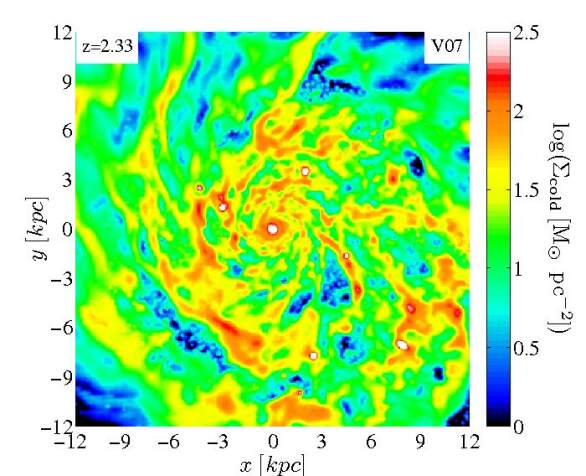
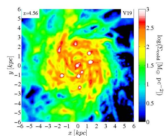
Figure 1: Face-on views of the surface density of cold mass in VELA-3 simulated discs showing giant clumps. Shown are V07 at $z\!=\!2.33$ (left) and V19 at $z\!=\!4.56$ (right). The cold mass is comprised of cold gas ($T\!<\!1.5\!\times\!10^{4}~{}{\rm K}$) and young stars ($<\!100~{}\,{\rm Myr}$). The disc radii are $R_{\rm d}\!=\!11.8$ and $3.2\,{\rm kpc}$ respectively. In both cases the disc half-thickness is $H_{\rm d}\!\sim\!R_{\rm d}/6$. The baryonic masses of the discs are $M_{\rm d}/(10^{10}M_{\odot})\!\sim\!3.50$ and $1.35$, and the fractions of cold-mass are $28\%$ and $33\%$ respectively. Both discs show giant clumps with masses $M_{\rm c}\!>\!10^{8}M_{\odot}$.

We use here the VELA suite of zoom-in cosmological simulations, 34 galaxies with halo masses $10^{11}-10^{12}M_{\odot}$ at $z\!\sim\!2$, which have been used to explore many aspects of galaxy formation at high redshift (e.g., Ceverino et al., 2014; Moody et al., 2014; Zolotov et al., 2015; Ceverino, Primack & Dekel, 2015; Inoue et al., 2016; Tacchella et al., 2016a, b; Tomassetti et al., 2016; Ceverino et al., 2016a, b; Mandelker et al., 2017; Dekel et al., 2020a, b; Ginzburg et al., 2021; Dekel et al., 2021). The simulations utilize the ART code (Kravtsov, Klypin & Khokhlov, 1997; Kravtsov, 2003; Ceverino & Klypin, 2009), which follows the evolution of a gravitating $N$-body system and the Eulerian gas dynamics with an AMR maximum resolution of $17.5-35\,{\rm pc}$ in physical units at all times. The dark-matter particle mass is $8.3\times 10^{4}M_{\odot}$ and the minimum mass of stellar particles is $10^{3}M_{\odot}$. The code incorporates gas and metal cooling, UV-background photoionization and self-shielding in dense gas, stochastic star formation, stellar winds and metal enrichment, and feedback from supernovae.

The thermal feedback model assumes that each stellar particle represents a single stellar population and injects the luminosity from supernovae and stellar winds as thermal heating, at a constant heating rate over $40\,{\rm Myr}$, the lifetime of the lightest star that explodes as a core-collapse supernova. (Ceverino & Klypin, 2009). The model adds non-thermal radiative pressure in regions where ionizing photons from massive stars are produced and trapped. In the VELA-3 version of the feedback model (RadPre in Ceverino et al., 2014), the radiative pressure is acting in cells that contain stellar particles younger than $5\,{\rm Myr}$ and whose gas column density exceeds $10^{21}\,{\rm cm}^{-2}$, as well as in these cell’s closest neighbors. In VELA-3 , the momentum driving efficiency is $\sim 3L/c$, which is comparable to the supernova contribution, but lower than in certain other simulations where the feedback is very strong (e.g., Genel et al., 2012; Oklopčić et al., 2017). Further details regarding the feedback and other sub-grid models in VELA-3 can be found in Ceverino et al. (2014) and Mandelker et al. (2017, M17).

The VELA-6 version of the radiative feedback (based on RadPre_IR in Ceverino et al., 2014) includes moderate trapping of infrared photons once that gas density in the cell exceeds $300\,{\rm cm}^{-3}$. In addition, the VELA-6 feedback model includes momentum injection from the expanding supernova shells and stellar winds (Ostriker & Shetty, 2011). A momentum of $10^{6}M_{\odot}\,{\rm km}\,{\rm s}^{-1}$ per star more massive than $8M_{\odot}$ is injected at a constant rate over $40\,{\rm Myr}$. The VELA-6 model also includes a factor of three boost in the injected momentum due to clustering of supernovae (Gentry et al., 2017), which is implemented in the form of non-thermal pressure as described in Ceverino et al. (2017). Further details regarding the feedback and other sub-grid models in VELA-6 can be found in Ceverino et al. (2014), Ceverino et al. (2017) and Ceverino et al. (in preparation).

M17 have analyzed the clumps in the VELA-3 galaxies as well as in counterparts that lacked the radiation pressure feedback (VELA-3 and VELA-2 respectively). They found that with radiation pressure a significant fraction of the clumps of $M_{\rm c}\!\leq\!10^{8}M_{\odot}$ are disrupted on timescales of a few free-fall times, while most of the more massive clumps survive. The migration inward of these long-lived clumps produced galacto-centric radial gradients in their properties, such as mass, stellar age, gas fraction and sSFR, which were found in Dekel et al. (2021) to be consistent with an analytic model and with observed clumps, distinguishing them from the short-lived clumps. However, in M17 the analyzed output times where separated coarsely by $\sim\!100\,{\rm Myr}$, which prevented a detailed study of the evolution of individual clumps. In the current study, we have re-simulated several of the VELA-3 galaxies, saving about ten snapshots per disc crossing time, with fine timesteps that can be as short as $\sim\!5\,{\rm Myr}$. Among these galaxies, five have L clumps (V07, V08, V19, V26, V27), and four others have only S clumps (V11, V12, V14, V25).

As in M17, the disc is defined as a cylinder with radius $R_{\rm d}$ and half height $H_{\rm d}$, containing 85% of the cold gas ($T\!<\!1.5\!\times\!10^{4}~{}{\rm K}$) and the young stars (ages $<\!100\,{\rm Myr}$) within $0.15R_{\rm v}$. The disc stars are also required to obey a kinematic criterion, that their specific angular momentum parallel to that of the disc, $j_{\rm z}$, is at least $70\%$ of the maximal possible value it could have given its galacto-centric distance, $r$, and orbital velocity, $v$, namely $j_{\rm max}\!=\!vr$.

The VDI phase typically follows a dramatic event of wet compaction into a star-forming “blue nugget”, that tends to occur when the halo mass is above $M_{\rm v}\!\sim\!10^{11.3}M_{\odot}$, and could happen at different redshifts, typically above $z\!=\!1$ (Zolotov et al., 2015; Tomassetti et al., 2016; Tacchella et al., 2016a, b, figure 2). An extended, long-lived clumpy disc, evolving to a clumpy ring, typically develops after the major compaction event, above the threshold mass where the disc is not disrupted by frequent mergers (Dekel et al., 2020a, b).

Figure 1 shows face on views of two simulated disks, V07 at $z\!=\!2.33$ and V19 at $z\!=\!4.56$, shortly after the start of their VDI phase. The figure shows the surface density of the cold mass, integrated over $\pm\!R_{\rm d}$ perpendicular to the disc, where $R_{\rm d}\!\simeq\!12$ and $3.2\,{\rm kpc}$ for V07 and V19 respectively. While these two discs are at very different redshifts, with different masses and sizes, both show giant star-forming clumps with masses $M_{\rm c}\!>\!10^{8}M_{\odot}$.

The gas fractions in the VELA-3 discs are somewhat lower than estimated in typical observed galaxies at similar redshifts. This has been discussed in detail in several papers which used these simulations (e.g., Zolotov et al., 2015; Tacchella et al., 2016b; Mandelker et al., 2017). While the VELA simulations are state-of-the-art in terms of high-resolution AMR hydrodynamics and the treatment of key physical processes at the subgrid level, they are not perfect in terms of their treatment of star-formation and feedback, much like other simulations. Star-formation tends to occur too early, leading to lower gas fractions later on. The stellar masses at $z\!\sim\!2$ are a factor of $\sim\!1.5\!-\!2$ higher than inferred for haloes of similar masses from abundance matching (e.g., Rodríguez-Puebla et al., 2017; Moster, Naab & White, 2018; Behroozi et al., 2019). However, for the purposes of the present study, the relatively low gas fractions during the peak VDI phase would only underestimate the actual accretion of fresh gas onto clumps during their migration, providing a lower limit on clump survival. The effect of gas fraction on clump properties and survival in simulated isolated discs is further discussed in Fensch & Bournaud (2021). In VELA-6 with the stronger feedback, the agreement with the stellar-to-halo mass ratio deduced from observations becomes better, but this comes at the expense of more dynamical destruction on the clump scales, which may or may not be more realistic. We do not attempt in this paper to decide between the different feedback models, but rather to study the effect of each on the survival and disruption of the giant clumps.

8.1.2 Clump analysis

Clumps are identified in 3D and followed through time following the method detailed in M17. Here we briefly summarize the main features. Clumps are searched for within a box of sides $4R_{\rm d}$ in the disc plane and height $4H_{\rm d}$ centered on the galaxy centre. Via a cloud-in-cell interpolation, the mass is deposited in a uniform grid with a cell size of $\Delta\!=\!70\,{\rm pc}$, two-to-three times the maximum AMR resolution. We then smooth the cell’s density, $\rho$, into a smoothed density, $\rho_{\rm w}$, using a spherical Gaussian filter of FWHM $\!=\!{\rm min}(2.5\,{\rm kpc},0.5R_{\rm d})$, defining a density residual ${\delta}_{\rm{\rho}}\!=\!(\rho\!-\!\rho_{\rm w})/\rho_{\rm w}$. Performed separately for the cold mass and the stellar mass, we adopt at each point the maximum of the two residual values. Clumps are defined as connected regions containing at least 8 grid cells with a density residual above ${\delta}_{\rm{\rho}}^{\rm min}\!=\!10$, making no attempt to remove unbound mass from the clump. We define the clump centre as the baryonic density peak, and the clump radius, $R_{\rm c}$, as the radius of a sphere with the same volume as the clump. The clump mass, however, is the mass contained in the cells within the connected region. Ex-situ clumps, which joined the disc as minor mergers, are identified by their dark matter content and the birth place of their stellar particles. They are not considered further here, where we focus on the in-situ clumps.

The SFR in the clumps is derived from the mass in stars younger than $30\,{\rm Myr}$, which is sufficiently long for fair statistics and sufficiently short for ignoring the stellar mass loss. Outflow rates from the clumps are measured through shells of radii $(R_{\rm c},R_{\rm c}+100\,{\rm pc})$. The gas outflow rate is computed by $\dot{M}_{\rm out}\!=\!\Delta^{-1}\sum_{i}V_{r}\,m_{i}$, with $\Delta\!=\!100\,{\rm pc}$, where the sum is over cells within the shell with $V_{r}\!>\!0$ and a 3D velocity larger than the escape velocity from the clump, $V^{2}\!>\!2GM_{\rm c}/R_{\rm c}$, and where $m_{i}$ is the gas mass in the cell. The gas accretion rate is computed in analogy to the outflow rates but with $V_{r}\!<\!0$ and no constraint on $V^{2}$. We note that this calculation involves large uncertainties.

Individual clumps, that contain at least 10 stellar particles, are traced through time based on their stellar particles. For each such clump at a given snapshot, we search for all “progenitor clumps” in the preceding snapshot, defined as clumps that contributed at least $25\%$ of their stellar particles to the current clump. If a given clump has more than one progenitor, we consider the most massive one as the main progenitor and the others as having merged, thus creating a clump merger tree. If a clump in snapshot $i$ has no progenitors in snapshot $i\!-\!1$, we search the previous snapshots back to two disc crossing times before snapshot $i$. If no progenitor is found in this period, snapshot $i$ is declared the initial, formation time of the clump, and for that clump $t$ is set to zero at that time. When tracing the evolution of a clump we refer to the main progenitor and consider the mergers to be part of the accretion onto the clump. The clump lifetime $\tau_{\rm c}$ is the age of the clump at the last snapshot when the clump is still identified.

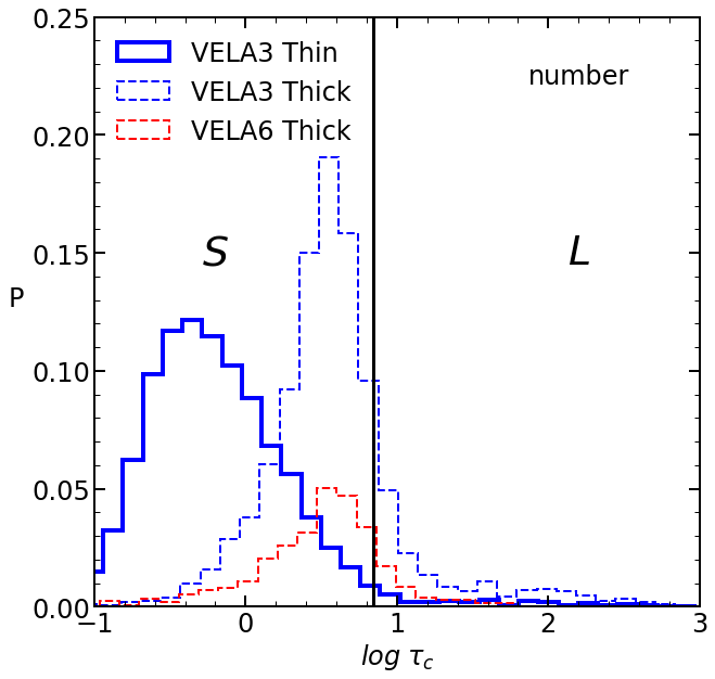
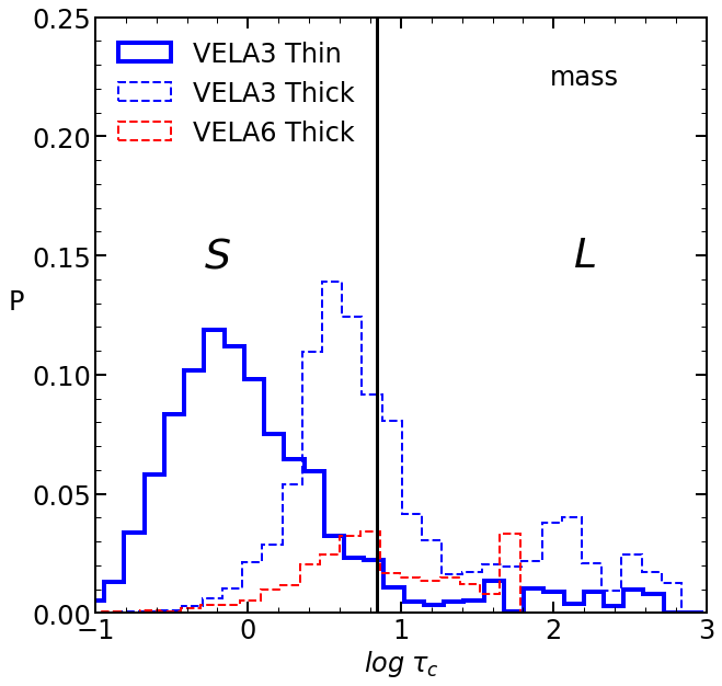
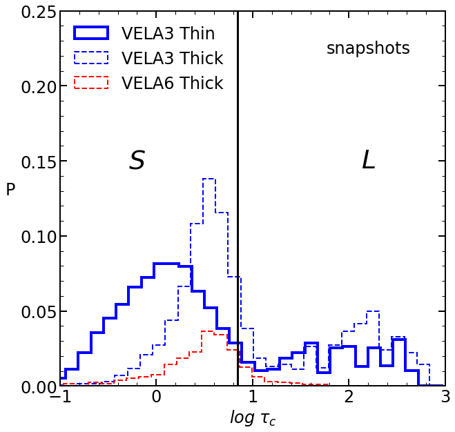
Figure 2: S vs L clumps. The distribution of lifetimes in units of free-fall times, $\tau_{\rm c}\!=\!t_{\rm c}/t_{\rm ff}$, for clumps in VELA-3 (blue solid line, normalized to unity). The minimum clump mass is set in this figure to $2\times 10^{7}M_{\odot}$. Left: Number of clumps. Middle: Weighted by clump mass. Right: Number at each snapshot, to be compared to observations. We see in the right panel a natural bimodality into S and L clumps, which we separate at $\tau_{\rm c}\!\sim\!7$. Also shown is the distribution of lifetimes in the VELA-6 simulations with the stronger feedback (dashed red), which is derived from the available coarser output timesteps of $\sim\!100\,{\rm Myr}$. The comparison with VELA-3 is performed using the same coarse timesteps in VELA-3 (dashed blue). The VELA-3 coarse-timestep histogram is independently normalized to unity, and the corresponding VELA-6 histogram is based on the same normalization as VELA-3 (the number of clumps from the coarse timesteps is lower than it is for the fine timesteps). We see that the coarse-timestep distributions are offset toward larger $\tau_{\rm c}$ (for reasons that are briefly discussed in the text), but the comparison of VELA-3 and VELA-6 using the coarse timesteps is fair. The VELA-6 simulations show less clumps than VELA-3, which are predominantly S clumps.

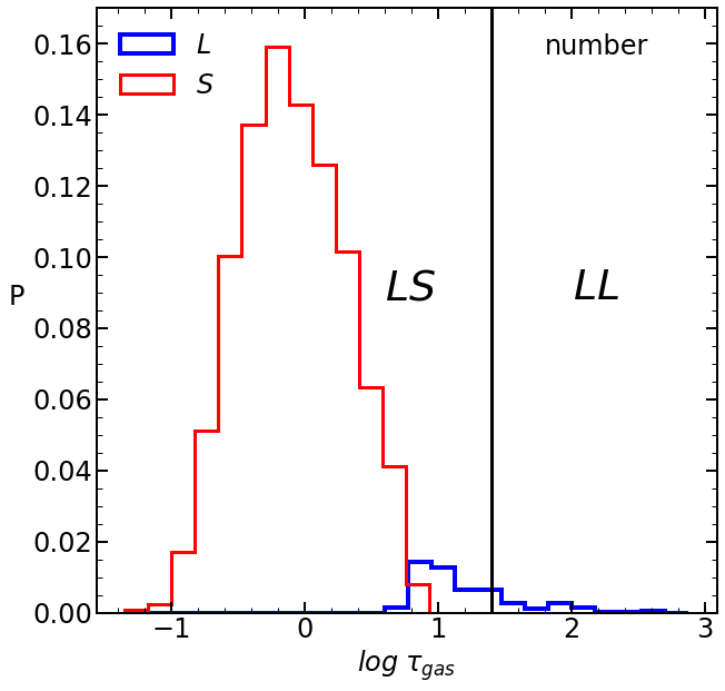
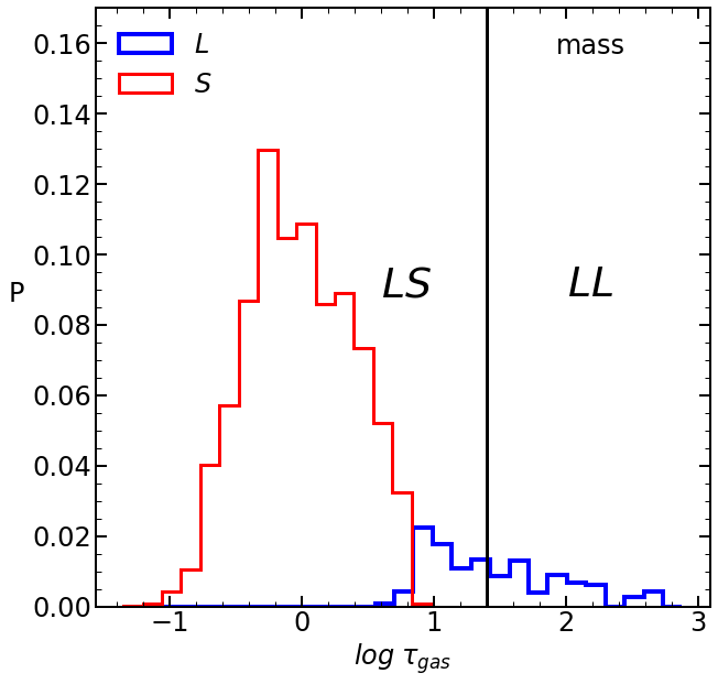
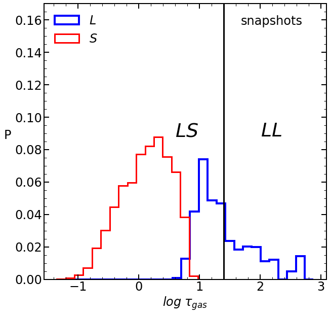
Figure 3: LS versus LL long-lived clumps in VELA-3. The distribution of $\tau_{\rm gas}$, the time when the clump have lost 90% of the gas it had at $\tau\!=\!4$ (if $\tau_{\rm c}\!<\!4$ then $\tau_{\rm gas}$ is set to equal $\tau_{\rm c}$). The minimum clump mass is set in this figure to $2\times 10^{7}M_{\odot}$. Left: Number of clumps. Middle: Weighted by clump mass. Right: Number at each snapshot, as observed. For the S clumps ($\tau_{\rm c}\!<\!7$) we have $\tau_{\rm gas}\!\simeq\!\tau_{\rm c}$. There is a natural division of the L clumps ($\tau_{\rm c}\!>\!7$) at $\tau_{\rm gas}\!\simeq\!25$ to LS clumps that lose most of their gas moderately early and LL clumps that keep most of their gas for tens of free-fall times.

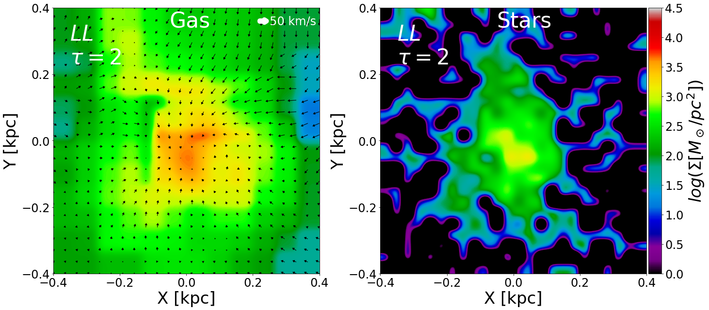
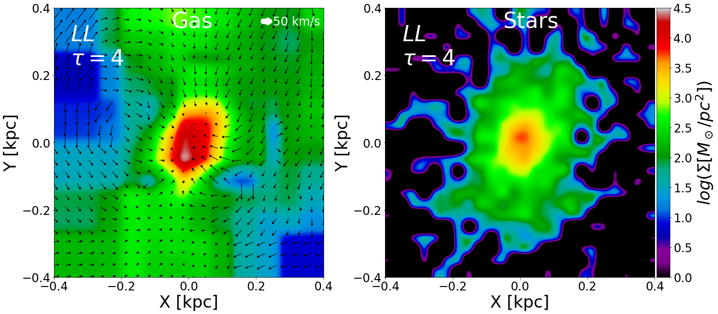
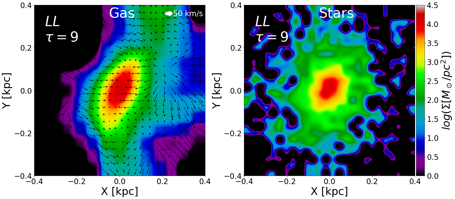
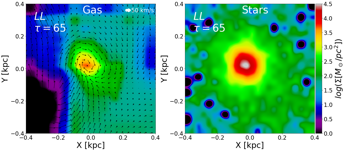
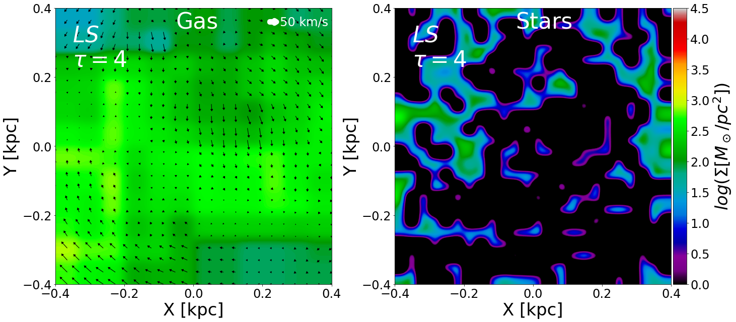
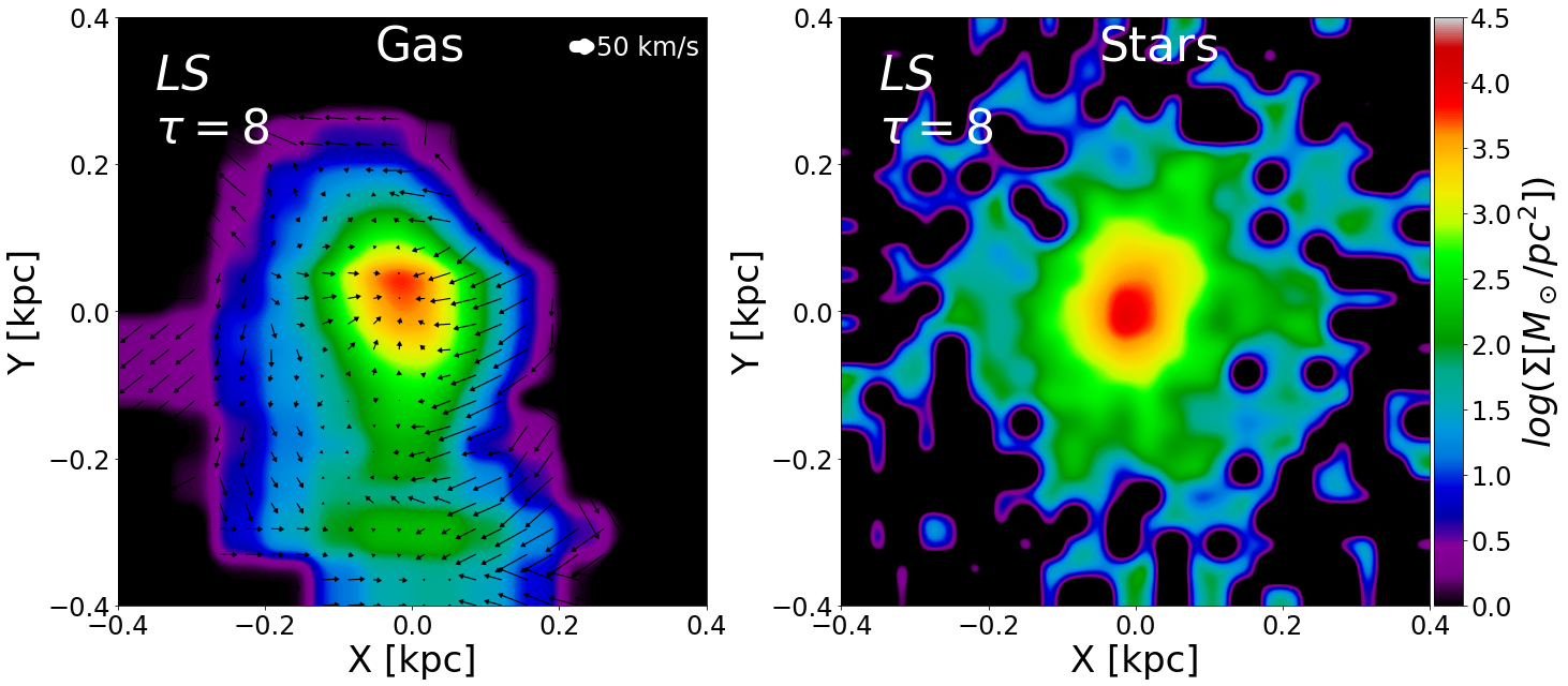
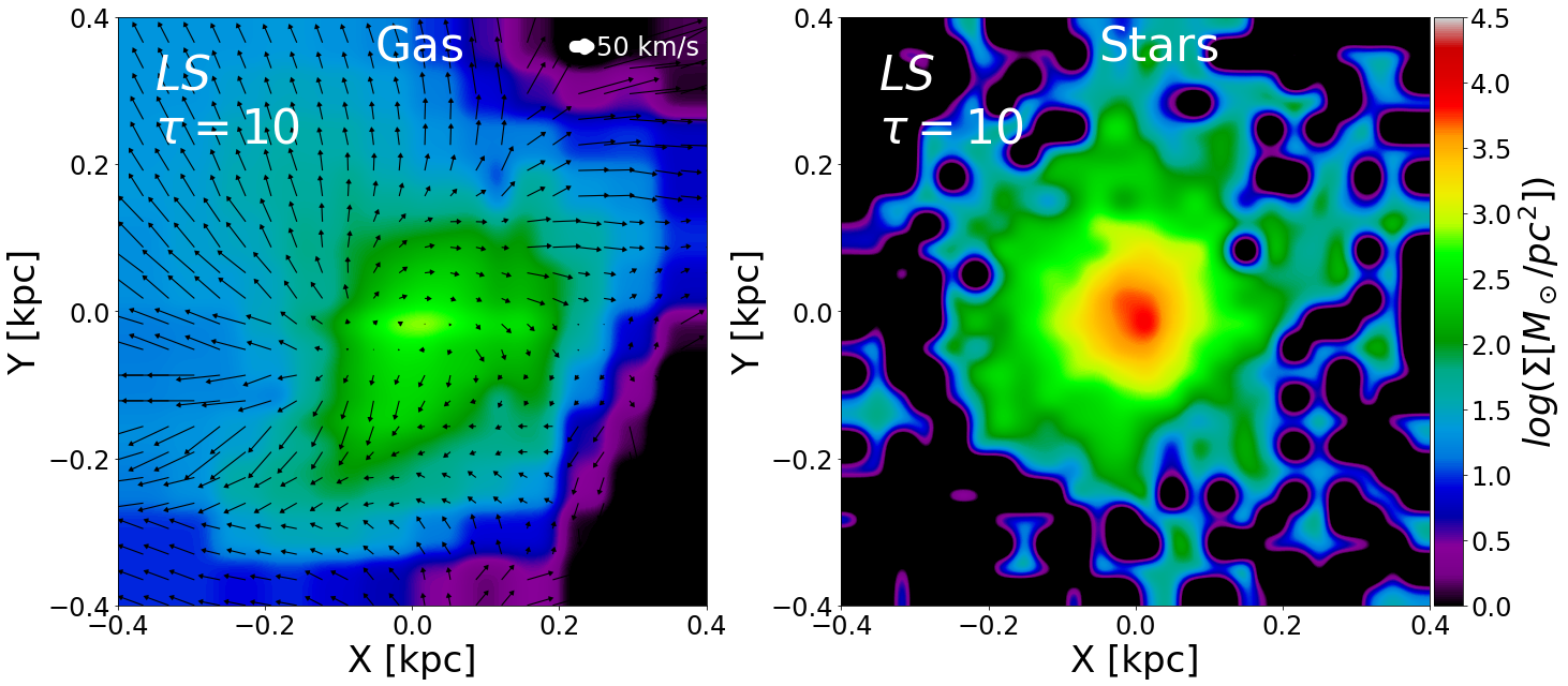
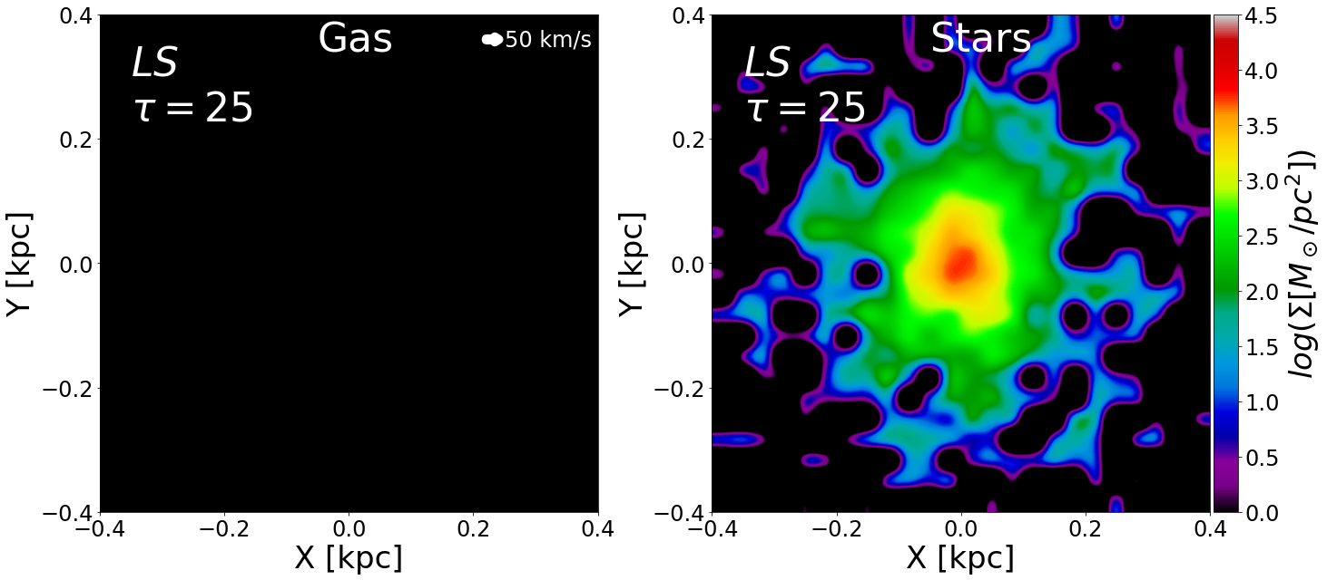
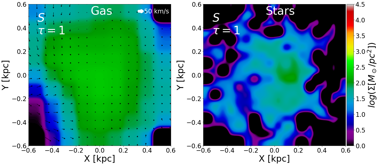
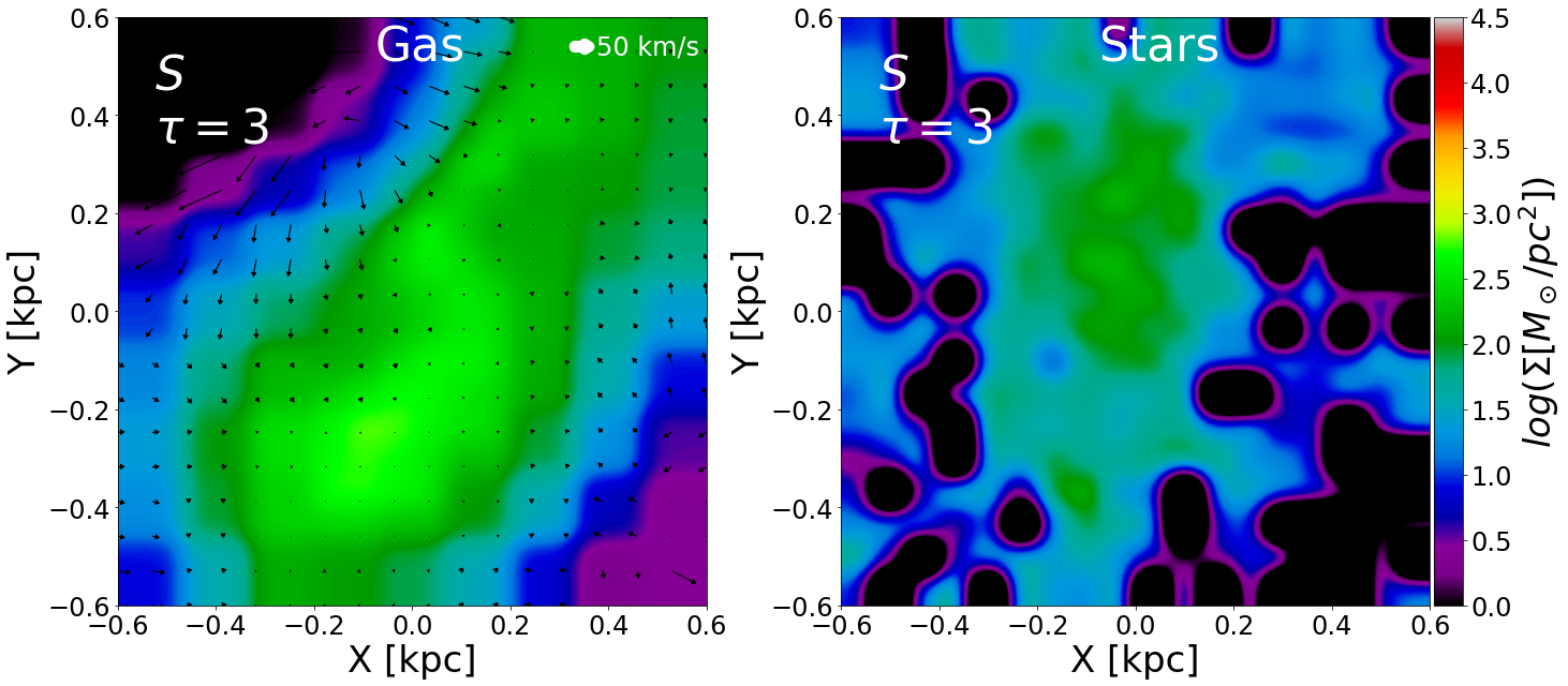
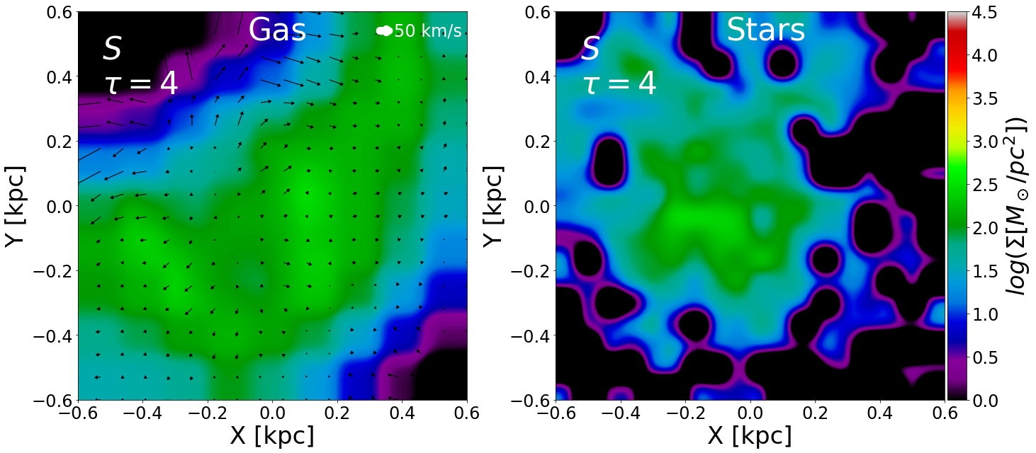
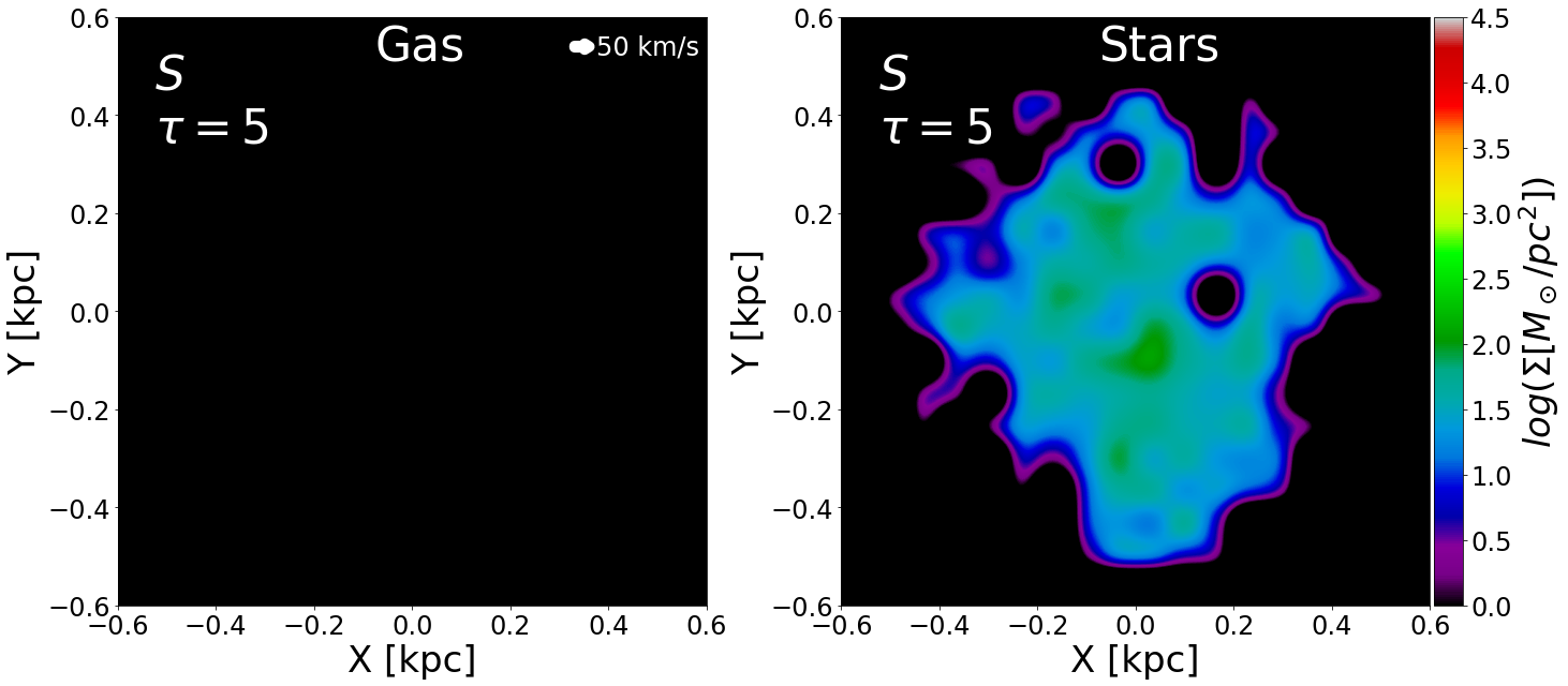
Figure 4: Images of gas (left) and stars (right) in examples of the 3 clump types at four times. Top: An LL clump at $\tau\!=\!2,4,9,65$, surviving both in stars and gas for tens of free-fall times. Middle: An LS clump at $\tau\!=\!4,8,10,25$, surviving in stars but losing all gas by $\tau\!\sim\!10$. Bottom: An S clump at $\tau\!=\!1,3,4,5$, losing all its gas and dispersing its stars by $\tau\!\sim\!5$.

8.2 Three clump types

The clumps for analysis were selected as follows. From the nine galaxies that were re-simulated with fine output timesteps, output snapshots were selected where the galaxies are discs with an axial ratio $R_{\rm d}/H_{\rm d}\!>\!3$. Clumps were selected for analysis only in snapshots when their baryonic mass is above a threshold mass $M_{\rm c}\!>\!10^{7}M_{\odot}$, with the additional requirement that their initial gas mass was $M_{\rm g}\!>\!10^{6}M_{\odot}$ at the snapshot when they were first identified.

As found in M17, the clumps in the VELA-3 simulations can be divided into two major classes based on their lifetimes. This is demonstrated in Fig. 2, which shows (in solid blue) the probability distribution of clump lifetimes in units of clump free-fall times, the latter being the mass-weighted average of $t_{\rm ff}$ over the clump lifetime. The distributions are shown in three different ways, corresponding to (a) clump number where each clump is counted once (left), (b) clump mass where each clump is counted once and the mass is the average over the clump lifetime (middle), and (c) clump number where each clump is counted at every snapshot in which it appears (right). The latter allows direct comparison to the distribution of clumps in observations. Here, the lifetimes were determined using the fine timesteps as opposed to the coarse timesteps used in M17. We see a bimodality into short-lived and long-lived clumps, which is emphasized in the right panel. We term them S and L clumps respectively, and separate here near a clump lifetime of $\tau_{\rm c}\!=\!t_{\rm c}/t_{\rm ff}\!\sim\!7$. The difference between the medians of the normalized $\tau_{\rm c}$ for S and L clumps, $\sim\!1.9$dex, reflects a large difference of $\sim\!1.4$dex in $t_{\rm c}$, aided by a smaller difference of $\sim\!0.5$dex in $t_{\rm ff}$ (see Fig. 7).

For a quick comparison of the clumps in the VELA-3 and VELA-6 simulations, with different feedback strengths, we appeal to a clump analysis using the coarser output timesteps of $\sim\!100\,{\rm Myr}$, which are the data currently available for VELA-6. Figure 2 shows in dashed lines the distributions of clump lifetimes using the coarse timesteps. The dashed VELA-3 histogram (blue) is normalized to unity, and the dashed VELA-6 histogram (red) is normalized based on VELA-3. We note in passing that for VELA-3 the distribution using the coarse timesteps is different from the fine-timestep distribution, for several reasons. First, the overall number of clumps is lower in the coarse-timestep analysis, despite having more galaxies in this analysis. This is because the fine timesteps allow more clumps to be identified, and because more zero-lifetime clumps are excluded in the analysis using coarse timesteps (termed ZLC in M17). Second, around $\tau_{\rm c}\!\sim\!10$ there are more clumps at a given $\tau_{\rm c}$ in the coarse-timestep analysis. This indicates that the corresponding histogram is shifted towards larger $\tau_{\rm c}$ values, despite the natural tenancy to measure larger lifetimes with finer timesteps. This shift is partly due to the way ages are assigned to S clumps at the first snapshot, especially if they are identified in one snapshot only, or because $t_{\rm ff}$ is somehow underestimated when averaged over less snapshots. The above comparison between the the fine and coarse timesteps is not relevant for our current aim to qualitatively compare between the clumps in VELA-3 and VELA-6 using the same coarse timesteps. We find that in VELA-6, with the stronger feedback, there are significantly fewer clumps, and a significantly smaller fraction of L clumps. This indicates that clump survival is a strong function of the feedback strength, as predicted by our model. A more detailed comparison between the clumps in the VELA-3 versus the VELA-6 simulations is deferred to Ceverino et al. (in preparation).

We next realize that the L clumps in VELA-3 can be divided into two sub-classes based on the way they lose their gas to outflows. This is demonstrated in Fig. 3, which shows for the S and L clumps in VELA-3 the distribution of $\tau_{\rm gas}$, the time when the clump has lost 90% of the gas mass it had at $\tau\!=\!4$. The latter is typically the time when the gas mass reaches a maximum. If $\tau_{\rm c}\!<\!4$ we set $\tau_{\rm gas}\!=\!\tau_{\rm c}$. Among the L clumps, one can identify a bi-modality into two types, separated near $\tau_{\rm gas}\!\sim\!25$, which we term LS and LL clumps respectively (the first L for the stars, the second S or L for the gas). The LL clumps are the long-lived clumps analyzed in M17 (sometimes together with the LS clumps) and in Dekel et al. (2021), which keep a significant fraction of their gas and a non-negligible SFR for many tens of free-fall times, till they complete their inward migration. The LS clumps, which we analyze here in detail, are in certain ways between the S clumps and the LL clumps. They lose most of their gas on a timescale of $\sim\!10$ free-fall times, while keeping a long-lived bound stellar component with only little SFR.

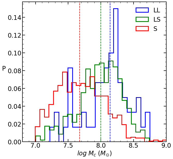
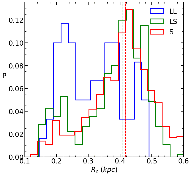
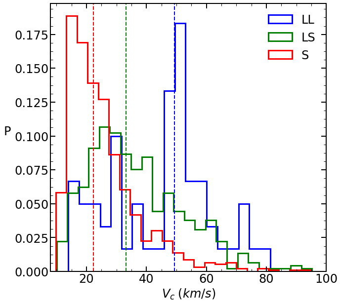
Figure 5: The probability distribution of the clump properties $M_{\rm c}$, $R_{\rm c}$ and $V_{\rm c}$, averaged over the early phase $\tau\!<\!4$, for the three clump types. Each clump is counted once. The medians are marked. There is a trend with mass from S through LS to LL, with the LL clumps typically above $10^{8}M_{\odot}$. The LL clumps tend to have smaller radii. As a result there is a clear trend with binding energy, via $V_{\rm c}$, from the loosely bound S clumps of $V_{\rm c}\!\sim\!20\,{\rm km}\,{\rm s}^{-1}$, through LS, to the strongly bound LL clumps of $V_{\rm c}\!\sim\!50\,{\rm km}\,{\rm s}^{-1}$.

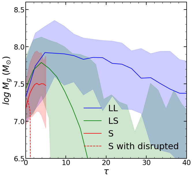
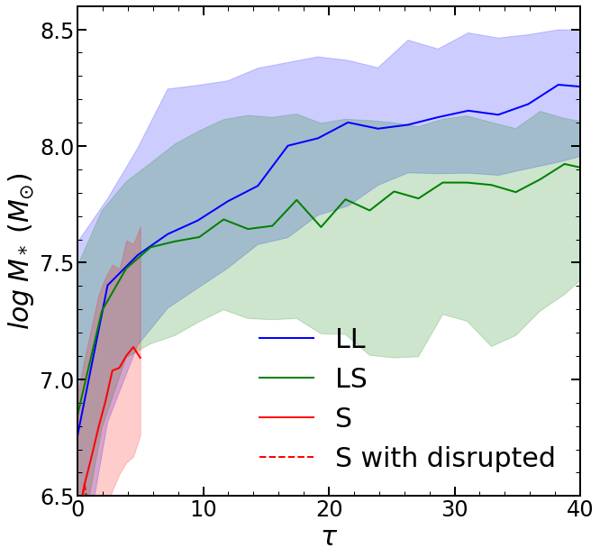
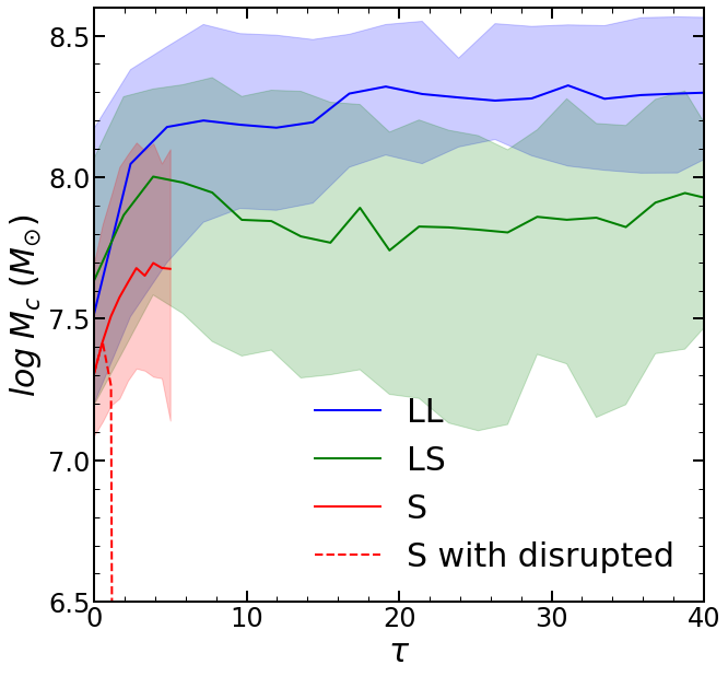
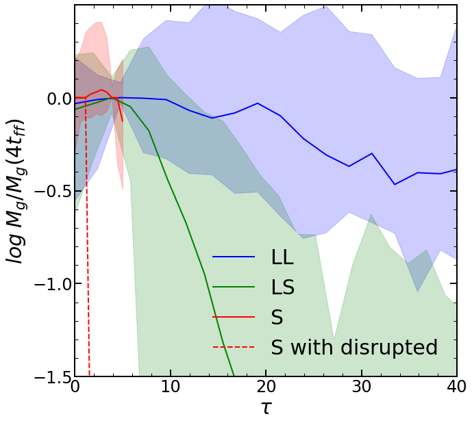
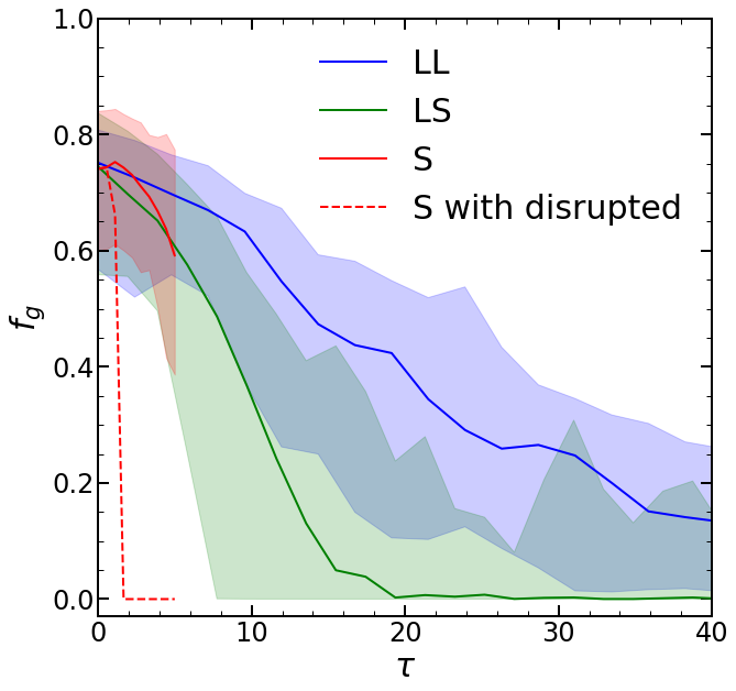
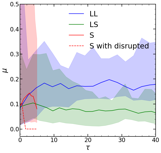
Figure 6: Time evolution of clump mass, $M_{\rm g}$, $M_{\rm s}$ and $M_{\rm c}\!=\!M_{\rm g}+M_{\rm s}$, for gas, stars and total, as a function of $\tau\!=\!t/t_{\rm ff}$. Shown are the medians and $1\sigma$ scatter for each of the three types. For the S clumps (red), the solid curve and shaded area refer to the small fraction of clumps that survive until the given time, while in the dashed curve the disrupted clumps are included with zero mass. The gas mass is also shown relative to its value at $\tau\!=\!4$, near its peak, and via the gas fraction $f_{\rm g}\!=\!M_{\rm g}/M_{\rm c}$. Also shown is $\mu$, the clump mass relative to the Toomre mass. The S clumps lose their gas in the first few free-fall times. The LS clumps lose most of their gas to outflows by $\tau\!\sim\!10$, but keep a bound stellar component. The LL clumps keep their gas and stars for tens of free-fall times.

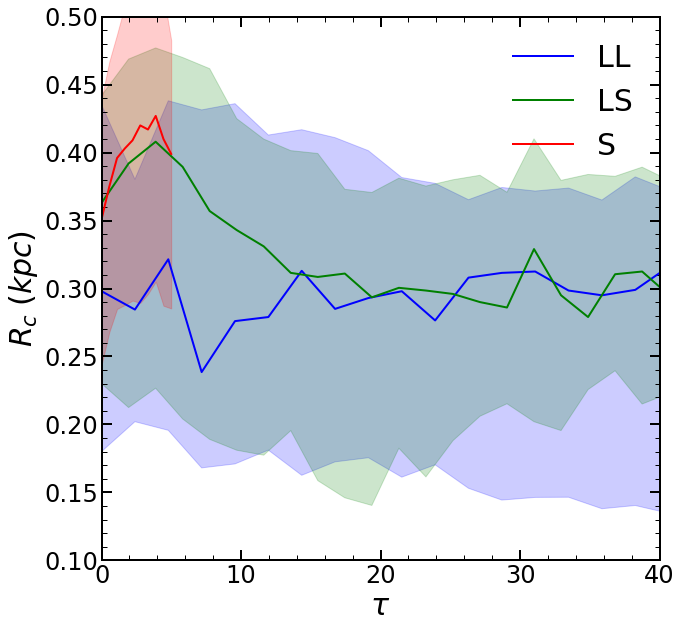
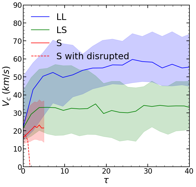
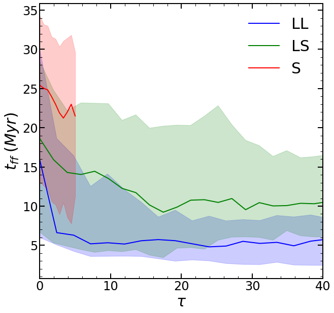
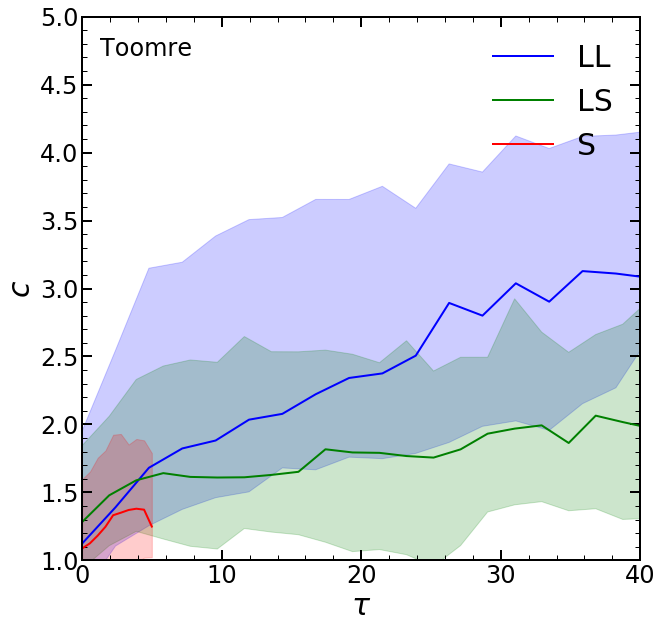
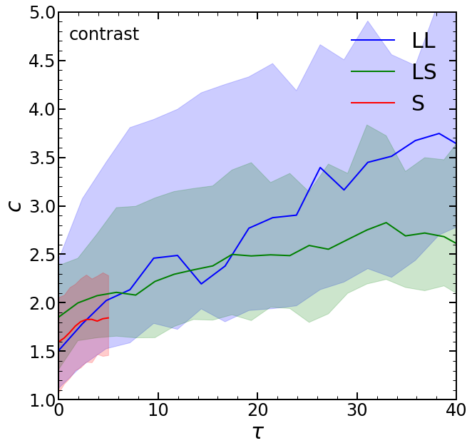
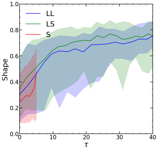
Figure 7: Evolution of clump size, velocity, and free-fall time at $\tau$. The density contrast $c$ is measured in two alternative ways, first by estimating the initial clump radius from the Toomre analysis (left), and second from the 3D density contrast between clump and disk (middle). The LL clumps tend to be smaller ($R_{\rm c}\!\sim\!300\,{\rm pc}$), more tightly bound $V_{\rm c}\!\sim\!50\,{\rm km}\,{\rm s}^{-1}$, and with short free-fall times ($t_{\rm ff}\!\sim\!5\,{\rm Myr}$). The S clumps are more diffuse and loosely bound ($R_{\rm c}\!\sim\!400\,{\rm pc}$, $V_{\rm c}\!\sim\!20\,{\rm km}\,{\rm s}^{-1}$, $t_{\rm ff}\!\sim\!23\,{\rm Myr}$). The contraction factor is somewhat higher for the LL clumps. The difference in clump shape between the clump types is marginal, with the S clumps slightly more elongated.

Figure 4 presents images of gas and stellar surface density in typical clumps of the three types in VELA-3. The LL clump shown at the top at times $\tau\!=\!2,4,9,65$ reveals a bound clump both in stars and gas all the way to $\tau\!=\!65$. On the other hand, in the LS clump shown in the middle at $\tau\!=\!4,8,10,25$, the gas has disappeared by $\tau\!=\!25$, while the significant stellar component remains largely unchanged till later times. The S clump shown at $\tau\!=\!1,3,4,5$ have lost all its gas already by $\tau\!=\!5$, and the stellar component becomes dilute at that time, to disappear soon thereafter.

The three clump types differ by many of their properties beyond the difference in life-time and gas depletion time that have been used for their classification. A few of these properties are shown in Fig. 5, through their distributions in VELA-3 during the first 4 free-fall times of each clump. In terms of clump mass, we see a weak systematic decrease of mass from LL to LS clumps, and a larger decrease into the S clumps, with medians $M_{\rm c}\!\sim\!10^{8.13},10^{8.0},10^{7.7}M_{\odot}$, the latter biased up by the selection threshold of $M_{\rm c}\!>\!10^{7}M_{\odot}$. In terms of clump radius, the LL clumps tend to be compact, with a median radius of $R_{\rm c}\!\sim\!320\,{\rm pc}$ (possibly affected by an effective threshold due to the simulation resolution), with the LS and S clumps both tending to be more diffuse, with medians at $R_{\rm c}\!\sim\!400\,{\rm pc}$. As a result, the clump virial velocity $V_{\rm c}$ tends to be the largest for LL clumps, intermediate for LS clumps, and smallest for S clumps, with medians of $V_{\rm c}\!\sim\!50,33,22\,{\rm km}\,{\rm s}^{-1}$ for LL , LS and S respectively.

The differences and similarities between the three clump types are explored in more detail by the time evolution of the relevant clump properties, for which the median and $\pm 34$ percentiles are shown as a function of time $\tau$ in Figs. 6 to 11. These detailed properties will serve us in the comparison with the analytic model of §2 to §7.

8.2.1 mass

Figure 6 presents the evolution of clump gas and stellar mass. Most of the S clumps disrupt within the first one or two free-fall times, so the S clumps referred to by the solid curve and shaded area represent the minority that survive for a little longer. The evolution of gas mass $M_{\rm g}$ is used for the basic classification of the L clumps into LL and LS clumps via $\tau_{\rm gas}$, which is to be used in the following figures. Referring to the medians of $M_{\rm g}(t)$, even the surviving S clumps have a median gas mass lower by a factor of $2\!-\!3$ than the L clumps. The LS clumps, after reaching a peak near $\tau$ of a few, show a steep decline where half the gas mass is lost by $\tau\!\sim\!8$ and practically no gas is left after $\tau\!\sim\!15$, while the LL clumps tend to keep most of their gas till $\tau\!\sim\!20$, with some of the LL clumps gaining gas mass during their evolution. This relative constancy of gas mass is associated with a roughly constant SFR. The stellar mass $M_{\rm s}$ for the two L types is similar till $\tau\!\sim\!10$, growing till $\tau\!\sim\!5$ and then gradually flattening off. At later times, the $M_{\rm s}$ of the LL clumps keeps growing roughly linearly with time, reflecting a constant SFR, while the $M_{\rm s}$ of the LS clumps is more constant due to the vaishing SFR (though its median is slowly rising, perhaps due to the larger masses of the clumps that survive longer, or due to accretion). The gas fraction provides an alternative quantity for the classification, with similar results to $M_{\rm g}$. All the clumps start with $f_{\rm g}\!\sim\!0.6\!-\!0.8$ and the LS and LL clumps differ after $\tau\!\sim\!4$, reaching $f_{\rm g}\!=\!0.5$ near $\tau\!\sim\!8$ and $\sim\!15$ respectively, with the LS clumps dropping to negligible gas fractions after $\tau\!\sim\!15$.

The median initial total mass of the L clumps at $\tau$ of a few is $M_{\rm c}\!\sim\!10^{8}M_{\odot}$, while for the S clumps it is smaller by a factor of $\sim\!3$. For the two types of L clumps, $M_{\rm c}$ is similar till $\tau\!\sim\!5$. After this time, while the median mass of the LL clumps is rather constant and even slowly rising, the mass of the LS clumps is gradually declining by a factor of $\sim\!3$ due to gas loss by outflows to a minimum mass near $\tau\!\sim\!20$, before it is slowly rising at later times. This could be due to stellar accretion or contamination by background disc stars. From $\mu(t)$, we learn that the median LL and LS clumps are of $\sim\!20\%$ and $\sim\!10\%$ of the Toomre mass, respectively.

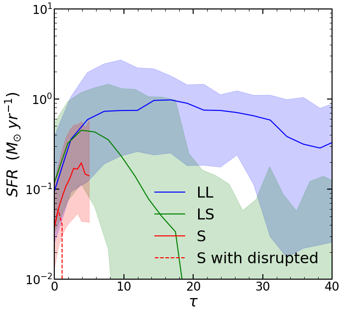
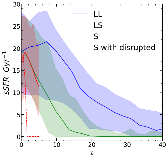
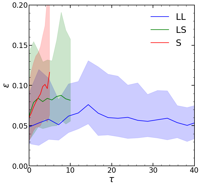
Figure 8: Evolution of SFR, sSFR and the SFR efficiency per free-fall time $\epsilon$ as measured over the whole clump. The SFR naturally follows the gas mass, so it is low for the S clumps, high for the LL clumps and roughly constant at $\!\lower 2.58333pt\hbox{$\;\buildrel<\over{\sim}\;$}\!\!1M_{\odot}\,{\rm yr}^{-1}$, and dropping for the LS clumps after a peak at $\tau\!\sim\!5$. The SFR efficiency is high, especially for the S and LS clumps, because it refers to the whole clump volume, while the star-forming region is actually more compact.

8.2.2 size and binding

Figure 7 highlights a basic continuous trend of $V_{\rm c}$ as a function of clump type, with peak median values in the initial phase $\tau\!=\!0\!-\!10$ of $V_{\rm c}\!\sim\!50,\,33$ and $20\,{\rm km}\,{\rm s}^{-1}$ for LL , LS and S clumps, respectively. This will directly affect the survivability parameter $S^{\prime}$, and will turn out to be the main distinguishing feature between the S and L clumps, as predicted in §6.1. The difference in $V_{\rm c}^{2}\!=\!GM_{\rm c}/R_{\rm c}$ may be due to a difference in $M_{\rm c}$ or $R_{\rm c}$ or both. Figure 7 shows that during the early phase the median radius is $R_{\rm c}\!\sim\!400\,{\rm pc}$ for the S and LS clumps, while it is $R_{\rm c}\!\sim\!300\,{\rm pc}$ for the LL clumps, with some clumps smaller than $200\,{\rm pc}$ (where the radius is probably overestimated due to resolution). This implies that the lower $V_{\rm c}$ for S clumps is predominantly due to the lower $M_{\rm c}$. As for the LS versus LL clumps, since the peak of $M_{\rm c}$ in the early phase differs by less than $0.2$ dex, the difference by a factor of almost two in the median $V_{\rm c}$ stems mostly from the similar difference in $R_{\rm c}$. This may be the basic difference between the LS and LL clumps, as discussed in §6.2. This difference in $R_{\rm c}$ is seen in the concentration $c$ as derived from the Toomre mass at $\tau\!\lower 2.58333pt\hbox{$\;\buildrel<\over{\sim}\;$}\!10$ (but less so in $c$ as estimated from the density contrast).

Figure 7 also shows a continuous trend in clump free-fall time, with a value at $\tau\!=\!5$ of $t_{\rm ff}\!\sim\!21,14$ and $6\,{\rm Myr}$ for S , LS and LL clumps, respectively. For the S clumps, the large $t_{\rm ff}$, reflecting a low density, is both due to the low $M_{\rm c}$ and the high $R_{\rm c}$. On the other hand, the difference between the two types of L clumps is mostly due to the difference in $R_{\rm c}$ and $c$.

As in M17, the clump shape elongation is measured via the axis ratio $\ell_{1}/\ell_{3}$, the distribution of which for the three clump types at $\tau<10$ is shown in Fig. 7. The median S clumps are slightly more elongated than the L clumps, $\ell_{1}/\ell_{3}\!\sim\!0.3$ versus $\sim\!0.4$, with some of the L clumps as round as $\ell_{1}/\ell_{3}\!\sim\!0.8$. The LS and LL clumps are not significantly different in shape.

8.2.3 SFR

Figure 8 presents the evolution of SFR and sSFR and the associated SFR efficiency per free-fall time $\epsilon$. For all types, the early-phase sSFR is high, at the level of $\sim\!20\,{\rm Gyr}^{-1}$, characteristic of a starburst in an initial stellar-poor clump. The median SFR in the S clumps is lower by a factor of three compared to the L clumps. Naturally the following decline in sSFR is associated with the decline in $M_{\rm g}$, which occurs in the S clumps first, then in the LS clumps, and later in the LL clumps. Figure 8 then shows an apparently surprising result concerning the SFR efficiency $\epsilon\!=\!\dot{M}_{\rm sf}\,t_{\rm ff}\,/M_{\rm g}$, where in the early phase it is $\epsilon\!\sim\!0.08$ and $0.055$ for the LS and LL clumps, respectively. This is mostly due to the larger $t_{\rm ff}$ for LS clumps, while $\dot{M}_{\rm sf}$ and $M_{\rm g}$ are similar. This is surprising because the SFR efficiency is argued based on observations to be in the same ballpark in all environments and redshifts (e.g. Krumholz, Dekel & McKee, 2012). One way to interpret this is that the SFR in the LS clumps actually occurs in regions denser than the average, near the clump centre or in sub-clumps, but this is not reproduced in the simulated clumps in which sub-clumps are not properly resolved.

Another possibility is that the higher $\epsilon$ is due to a more efficient mode of bursty star formation in the LS clumps, e.g., due to shocks induced by clump mergers, intense accretion, or strong tidal effects. An inspection of Fig. 3 of Krumholz, Dekel & McKee (2012), which is an accumulation of star-forming regions in galaxies in different environments and redshifts, and focusing on high-redshift galaxies (blue symbols), one can see that the starbursts (open symbols), which are likely to represent mergers, have $\epsilon$ values that are systematically higher than those of the normal discs (filled symbols), by a factor of a few. Referring to the discussion in §6.2, these inferred mergers can be associated with an increase in $f_{\rm grav}$ and $f_{\rm sn}$ compared to the LL clumps, which makes $S^{\prime}$ smaller and thus can explain the early disruption of the LS clumps. Such an excess of mergers, accretion and tidal effects can be associated with the larger radii of the LS clumps, introducing a larger cross-section for mergers and capture of gas within the clump Hill sphere, as well as stronger tidal effects.

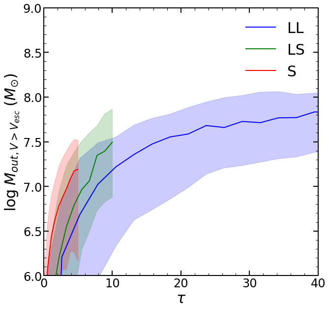
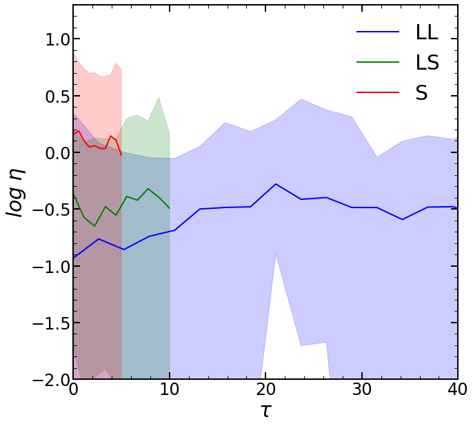
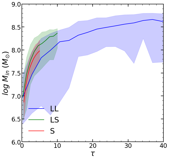
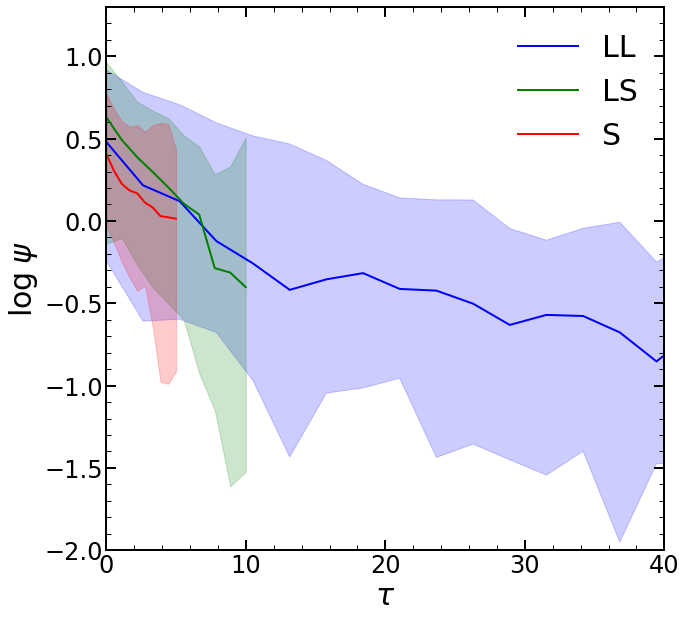
Figure 9: Evolution of outflow and inflow. Shown are the cumulative masses in outflow and inflow, as well as the corresponding parameters $\eta$ and $\psi$ and the outflow velocity $V_{\rm out}$. The outflows are most efficient for the S clumps and least efficient for the LL clumps, with medians in the early phase of $\eta\!\sim\!1.2,0.3,0.2$ respectively. The inflows are more similar between the clump types.

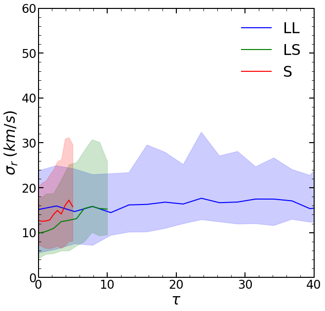
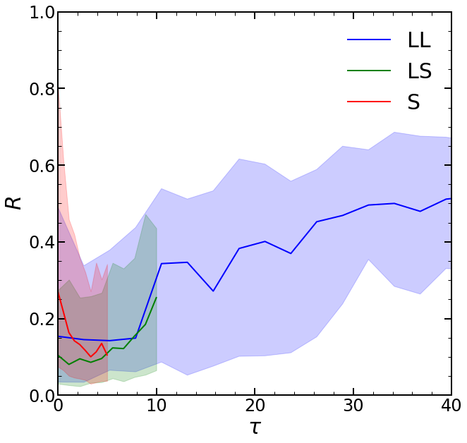
Figure 10: Evolution of clump internal kinematics, the rotation velocity $V_{\rm rot}$, the radial velocity dispersion $\sigma_{r}$, and the rotation support parameter $R\!=\!V_{\rm rot}^{2}/V_{\rm c}^{2}$. The LL clumps have a larger rotation component, consistent with the higher contraction factor.

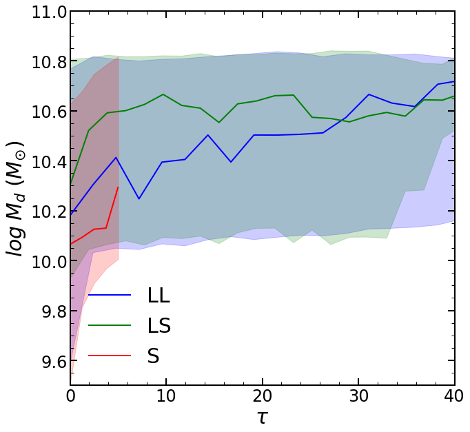
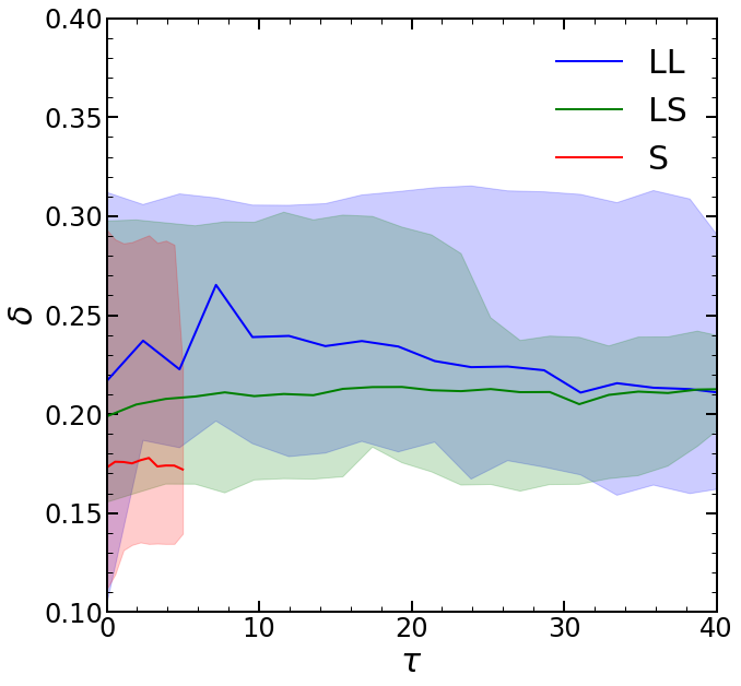
Figure 11: Evolution of disc mass $M_{\rm d}$ and mass fraction $\delta$, and clump position in the disc in the radial and vertical directions. The disc fraction for galaxies hosting LL clumps is somewhat higher, indicating a stronger disc instability with more massive clumps. The radial migration rate for LS clumps seems higher in terms of $\tau$, but this is an artifact of the longer free-fall times for these clumps. There is no significant difference in the effective $z$ positions of the different clump types.

8.2.4 outflow and inflow

Figure 9 shows the evolution of gas outflows from and inflows into the clumps. During the early phase, the outflowing mass is significantly smaller than the clump mass, as predicted in §3.1. As expected, the outflows in the S clumps are the strongest, with a median larger by a factor of $\sim\!3$ compared to the L clumps. The outflow is larger by a factor of $\sim\!2$ in the LS clumps compared to the LL clumps, leading to a smaller $S$ in eq. (1). The outflow mass loading factor varies systematically in a corresponding way, with a median of $\eta\!\sim\!1.2,0.3,0.2$ for S , LS and LL clumps respectively at $\tau\!<\!10$. The inflow parameter $\psi$ is defined following eq. 9 of Dekel et al. (2021) (where it is termed $\alpha$),

$$\psi=2\,\dot{M}_{\rm in},t_{\rm d}/M_{\rm c}\,.$$ (69)

Here $\dot{M}_{\rm in}$ is measured in analogy to $\dot{M}_{\rm out}$, in a shell of radii $(R_{\rm c},R_{\rm c}+100\,{\rm pc})$, requiring $V_{r}\!<\!0$ but not constraining the absolute value of $V$. The inflowing mass during the early phase is also larger in the LS clumps than in the LL clumps by a factor $\sim\!2$, with the S clumps similar to and slightly smaller than the LS clumps. The associated value of $\psi$ is larger for the LS clumps than the LL clumps until $\tau\!\sim\!0.7$, with the S clumps similar to the LL clumps. The inflowing mass is consistent with more mergers and intense accretion involved in the early phases of the LS clumps, and an associated higher $f_{\rm grav}$, leading to a lower $S^{\prime}$.

8.2.5 kinematics

Figure 10 shows that at the early times the clumps are not rotation supported, with the LL clumps somewhat more supported by rotation than the LS clumps. With $V_{\rm rot}$ the mass-weighted rotation velocity, the rotation-support parameter is $R\!=\!V_{\rm rot}^{2}/V_{\rm c}^{2}\!\sim\!0.15$ and $0.1$ for the LL and LS clumps respectively. This is consistent with the larger contraction factor $c$ for LL clumps, as predicted in eq. (31) in §3.3, if angular momentum is conserved during clump collapse. Both $V_{\rm rot}$ and $\sigma_{r}$ are larger for the LL clumps, though the difference in $V_{\rm rot}$ is slightly larger. We note in passing that the LL clumps gradually become more rotation supported at later times.

8.2.6 disc

Figure 11 refers to the clump positions in the host galactic discs. The initial values of $r/R_{\rm d}$ and $|z|/H_{\rm d}$ (at $\tau\!\sim\!2$) are similar for the different clump types, indicating that the differences among the types are not largely due to the position of formation within the disc. The two types of L clumps migrate radially inwards at a rather slow pace, in the ball park of the various theoretical predictions (Dekel, Sari & Ceverino, 2009; Krumholz & Burkert, 2010; Krumholz et al., 2018; Dekel et al., 2020b). The non-zero values of $|z|/H_{\rm d}$ and their large scatter reflect the fact that the clumps oscillate about the disc plane. While the median position of the LS clumps is at $|z|\!\sim\!\!0.3H_{\rm d}$, the LL clumps get somewhat closer to the disc mid-plane by $\tau\!\sim\!5$, and keep a median distance of $|z|\!\sim\!\!0.2H_{\rm d}$ or less till $\tau\!\sim\!30$.

The median LS discs tend to be more massive than the LL disks, but the disc mass fraction compared to the total mass including stars and dark matter, $\delta$, is somewhat larger for the LL clumps. This is consistent with a shorter inward migration time in units of disc dynamical time for the LL clumps (Dekel, Sari & Ceverino, 2009). The weak opposite trend in $r(t)/R_{\rm d}$ in terms of $\tau$ is probably because $t_{\rm ff}$ is larger for the LS clumps.

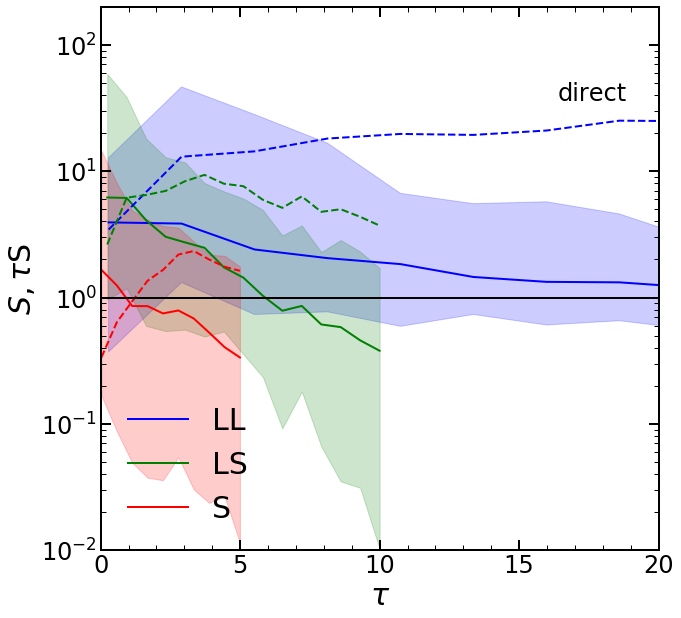
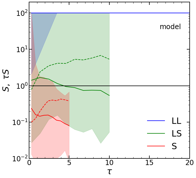
Figure 12: Time evolution of $S$ (solid) and $\tau S$ (dashed), the quantities that evaluate clump survivability against gas loss and total disruption, respectively, for the three clump types. Left: $S$ as measured directly from the simulations from $M_{\rm out}$, eq. (53). Right: $S$ as measured from the physical parameters assuming energy balance, eq. (54) (version 2 with $\gamma\!=\!1$). Values larger than 100 are set to 100. During the first few dynamical times, the median $S$ values are significantly smaller for the S clumps compared to the L clumps, consistent with the expected disruption of the S clumps compared to the survival of the L clumps. The median $S$ for the LS clumps declines to below unity after $\tau\!\sim\!5\!-\!10$, while for the LL clumps it remains above unity till $\tau\!\sim\!20$ and beyond. The median values of $\tau S$ distinguish between the S and LS clumps, consistent with the destiny of complete disruption for the S clumps and only gas removal for the LS clumps, leaving behind bound stellar LS clumps.

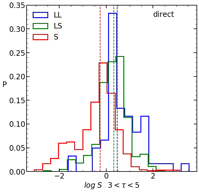
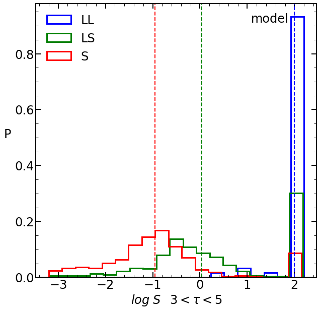
Figure 13: The probability distributions of the survivability parameter $S$ for the three clump types, as in Fig. 12 but during $\tau\!=\!3\!-\!5$. Left: $S$ measured directly from the simulations, eq. (53). Most of the L clumps have $S\!>\!1$ and most of the S clumps have $S\!<\!1$, with the medians near $3$ and $0.5$ respectively. Right: $S$ measured from the physical parameters, eq. (54) (version 2 with $\gamma\!=\!1$). Here all the LL clumps have $S\!\gg\!1$, the LS clumps have $S$ distributed about unity, and the vast majority of the S clumps have $S\!\ll\!1$, with the medians $\gg\!1$, $\sim\!1$ and $\sim\!0.1$ respectively.

9 Theory versus simulations

Using the simulations, we compute the survivability parameter $S$ as a function of time since clump formation for the simulated clumps of the three types. We compute $S$ in two alternative ways, which we term $S_{\rm dir}$ and $S_{\rm mod}$. First, directly from the simulations, we determine $S$ from the measured $M_{\rm out}(t)$, $M_{\rm c}$ and the correction factor $p$, using the definition of $S$ in eq. (53). Alternatively, we compute $S$ from eq. (54), based on our model assuming energy conservation and the different sources of energy gain and loss, using the measured $V_{\rm c}$ and the factors $f_{\rm sn}$ (eq. 56), $f_{\rm grav}$ (eq. 58) and $f_{\rm dis}$ (eq. 57).

Figure 12 shows the evolution of $S$ and of $\tau S$ for the three clump types as computed by the two methods. Recall that $S$ is supposed to measure the clump survivability against losing its gas mass by supernova feedback, thus distinguishing between S and L clumps by $S$ values below and above unity, respectively. The product $\tau S$ is expected to measure the clump survivability against total disruption versus partial mass loss followed by a bound stellar system, thus distinguishing between S and LS clumps, by $\tau S$ values below and above unity, respectively. Inspecting the medians, we see that during the first few dynamical times $S$ is significantly smaller in the S clumps compared to the L clumps, as expected. The median of $S$ for the LS clumps, which starts well above unity at early times, declines to below unity after $\tau\!\sim\!5\!-\!10$, while for the LL clumps it remains above unity till $\tau\!\sim\!20$ or further, as anticipated. The median values of $\tau S$ indeed distinguish between the S clumps that will disrupt completely and the LS clumps that will keep their stars bound, as expected.

Viewing the survivability parameter from a different angle, Fig. 13 shows the probability distributions of $S$ for the three clump types at the early phase $\tau\!=\!3\!-\!5$. The values of $S$ as measured directly from the simulations yield that most of the L clumps have $S\!>\!1$ and most of the S clumps have $S\!<\!1$, with the medians near $3$ and $0.5$ respectively. The calculation of $S$ based on the model assuming conservation of energy yields that all the LL clumps have $S\!\gg\!1$, the LS clumps have $S$ distributed about unity, and the vast majority of the S clumps have $S\!\ll\!1$, with the medians near $\gg\!1$, $1$ and $0.1$ respectively. We conclude that, in general, $S$ serves its purpose as a predictor of clump types.

Comparing the measured $S$ and $\tau S$ by the two methods, we note that the medians of these quantities indeed distinguish between the clump types in both cases. We note however that in the direct calculation using eq. (53) the median values of $\tau S$ for the S clumps are slightly above unity. This may reflect the uncertainty in measuring $M_{\rm out}$. In particular, our assumption that $V_{\rm out}^{2}\!\simeq\!2V_{\rm c}^{2}$ that enters eq. (6) may be inaccurate. If we parametrize $V_{\rm out}^{2}=f_{\rm esc}\,2V_{\rm c}^{2}$, we obtain $S_{\rm mod}\!\propto\!f_{\rm esc}$. A value of $f_{\rm esc}\!\sim\!2$, or a range of values for the different clump types, as in Fig. 9, may reduce the apparent differences between $S_{\rm dir}$ and $S_{\rm mod}$. Such refinements of the model are deferred to future work.

10 Conclusion

Energetics considerations lead to a physical criterion for the survival versus disruption of the giant clumps that dominate high-redshift galactic discs. Depending on the disc and clump properties, the model predicts populations of short-lived clumps (S) that lose their gas in a few free-fall times during formation and long-lived clumps (L) that keep their gas for longer periods. The latter are of two types, those that lose most of their gas to outflows in $\!\lower 2.58333pt\hbox{$\;\buildrel<\over{\sim}\;$}\!\!10$ free-fall times but keep gas-deficient, long-lived, bound stellar clumps (LS), and those that keep most of their baryons for tens of free-fall times and remain star forming roughly at a constant rate (LL).

Our model introduces a survivability parameter $S$, which can predict the level of survivability against gas loss at a given time based on the clump and disc properties and physical parameters that characterize the SFR and feedback, distinguishing between S and L clumps. The quantity $\tau S$, where $\tau\!=\!t/t_{\rm ff}$, then predicts the survivability against total disruption by rapid gas loss, distinguishing S from LS clumps. These quantities are defined as

$$S=\frac{0.5\,M_{\rm c}}{M_{\rm out}(t)}\,,\quad\tau S\simeq\frac{0.5\,M_{\rm c}}{\dot{M}_{\rm out}t_{\rm ff}}\,.$$ (70)

Thus, the distinction between the three clump types based on the survivability parameter $S$ during the first few clump free-fall times is as summarized in Table 1, namely S clumps have $S\!<\!1$ and $\tau S\!<\!1$, LS clumps have $S\!\lower 2.58333pt\hbox{$\;\buildrel<\over{\sim}\;$}\!1$ but $\tau S\!\lower 2.58333pt\hbox{$\;\buildrel>\over{\sim}\;$}\!1$, and LL clumps have $S\!>\!1$ and $\tau S\!>\!1$. The model successfully reproduces the distribution of clump properties in cosmological simulations, and provides a physical basis for the existence of the three clump types in these simulations.

The model considers the balance between the energies supplied by supernova feedback and by gravitational interactions against the energy required for overcoming the clump binding energy, the energy carried away by outflows, and the dissipative losses of turbulence. The supernova input is based on a generalization of the analysis by Dekel & Silk (1986). The clumps are assumed to form by Toomre instability within VDI discs (Dekel, Sari & Ceverino, 2009). If they manage to contract sufficiently, the clumps are assumed to reach virial and Jeans equilibrium (Ceverino et al., 2012).

Three clump types
Type	Gas loss	Stars	$S$	$\tau S$
Short-lived S	$\sim\!t_{\rm ff}$	none	$S\!<\!1$	$\tau S\!<\!1$
Long-lived stars LS	$\sim\!10t_{\rm ff}$	bound	$S\!\lower 2.58333pt\hbox{$\;\buildrel<\over{\sim}\;$}\!1$	$\tau S\!\lower 2.58333pt\hbox{$\;\buildrel>\over{\sim}\;$}\!1$
Long-lived LL	$\gg\!t_{\rm ff}$	bound	$S\!>\!1$	$\tau S\!>\!1$

Table 1: The three clump types are distinguished by the survivability parameter during the first few clump free-fall times. $S\!<\!1$ predicts significant gas loss, while $\tau S\!<\!1$ predicts rapid gas loss that leads to total disruption.

We obtain $S\!\simeq\!(S^{\prime-1}\!-\!1)^{-1}$, namely the critical value of $S^{\prime}$ corresponding to $S\!=\!1$ is $S^{\prime}=0.5$. For a simple interpretation of the main results, considering only the balance between the deposited supernova energy and the clump binding energy, we approximate near the first free-fall time

$$S^{\prime}\simeq\frac{E_{\rm vir}}{E_{\rm sn}}\simeq\frac{V_{\rm c,50}}{e_{51}}\,.$$ (71)

The linear dependence on the clump circular velocity $V_{\rm c}$ results from the fact that $E_{\rm vir}\propto V_{\rm c}^{2}$ while $E_{\rm sn}\propto V_{\rm c}$ (via its dependence on the velocity dispersion in the clump ISM). The survivability is thus a strong function of the clump circular velocity (which is correlated with the clump mass) and the feedback strength as formulated via $e_{51}$. In turn, a Toomre analysis connects the clump circular velocity to the disc properties via

$$V_{\rm c}\propto f_{\rm g}\,V_{\rm d}\,.$$ (72)

This introduces strong gas-fraction dependence and disc mass dependence for the clump survival via $S$.

If the strength of ejective feedback is at a moderate level, we find that L clumps are likely to exist, with a binding energy that is characterized by a circular velocity $V_{\rm c}\!\sim\!50\,{\rm km}\,{\rm s}^{-1}$, at or above a clump threshold mass $\sim\!10^{8}M_{\odot}$. The L clumps tend to form in discs of $V_{\rm d}\!\geq\!200\,{\rm km}\,{\rm s}^{-1}$, corresponding at $z\!\sim\!2$ to stellar masses above $\sim\!10^{9.3}M_{\odot}$ and galactic halo masses above $\sim\!10^{11.3}M_{\odot}$, which are typically required for long-lived discs against disruption by mergers in an orbital time (as predicted by Dekel et al., 2020a). L clumps are predicted to favor gas fractions $\!\geq\!\!0.3$ and more so when the central mass of bulge and dark matter is small. The L clumps prefer to form at high redshifts, peaking at $z\!\sim\!2$.

On the other hand, the likelihood of L clumps is severely reduced if the ejective feedback is stronger, e.g., if the effective energy per supernova is well above the standard value due to clustering of supernovae, if very strong radiative feedback is included, if the stellar initial mass function is top-heavy, or if the star-formation-rate efficiency is higher than commonly assumed on average. Simulations with varying levels of ejective feedback indeed permit L clumps with different efficiencies.

The division of the L clumps into two sub-populations is demonstrated in the simulations. The model may explain the existence of LS clumps by a smaller contraction factor during formation and stronger external gravitational effects, where clump mergers may increase the SFR efficiency. This is compared to the more compact LL clumps that retain most of their baryons for tens of free-fall times.

A word of caution concerns the fact that we have modeled the overall stellar feedback based on the supernova feedback component. This is a first crude treatment that should be improved by detailed considerations of the other feedback mechanisms, such as radiative feedback and stellar winds. Furthermore, our current treatment ignored the clustering of supernovae, which is expected to increase the deposited feedback energy in low-mass star clusters and to decrease it in massive clusters (Gentry et al., 2017). These should be improved in future studies.

Our findings emphasize a challenging general feedback puzzle. While the model successfully predicts that for a moderate feedback strength the massive clumps are long-lived, when implemented in simulations (such as VELA-3) this moderate feedback leads to an overestimate of the stellar-to-halo mass ratio as estimated from observations via abundance matching (Rodríguez-Puebla et al., 2017; Moster, Naab & White, 2018; Behroozi et al., 2019). On the other hand, simulations with stronger feedback (such as VELA-6), which better match the stellar-to-halo mass ratio, practically fail to reproduce long-lived clumps. If the observed massive clumps are long-lived, as indicated, for example, by their not-so-young stellar ages and the gradients in clump properties that are consistent with VDI-driven clump radial migration (Dekel et al., 2021), then one is challenged to come up with more sophisticated feedback mechanisms. The feedback should be more preventive and less ejective, such that it efficiently suppresses star formation while it is less destructive in terms of ejecting gas from the clumps.

DATA AVAILABILITY

Data and results underlying this article will be shared on reasonable request to the corresponding author.

References

- Agertz, Teyssier & Moore (2009) Agertz O., Teyssier R., Moore B., 2009, MNRAS, 397, L64
- Behroozi et al. (2019) Behroozi P., Wechsler R. H., Hearin A. P., Conroy C., 2019, MNRAS, 488, 3143
- Botticella et al. (2017) Botticella M. T. et al., 2017, A&A, 598, A50
- Bournaud, Elmegreen & Elmegreen (2007) Bournaud F., Elmegreen B. G., Elmegreen D. M., 2007, ApJ, 670, 237
- Cacciato, Dekel & Genel (2012) Cacciato M., Dekel A., Genel S., 2012, MNRAS, 421, 818
- Ceverino et al. (2016a) Ceverino D., Arribas S., Colina L., Rodríguez Del Pino B., Dekel A., Primack J., 2016a, MNRAS, 460, 2731
- Ceverino, Dekel & Bournaud (2010) Ceverino D., Dekel A., Bournaud F., 2010, MNRAS, 404, 2151
- Ceverino et al. (2012) Ceverino D., Dekel A., Mandelker N., Bournaud F., Burkert A., Genzel R., Primack J., 2012, MNRAS,
- Ceverino & Klypin (2009) Ceverino D., Klypin A., 2009, ApJ, 695, 292
- Ceverino et al. (2014) Ceverino D., Klypin A., Klimek E. S., Trujillo-Gomez S., Churchill C. W., Primack J., Dekel A., 2014, MNRAS, 442, 1545
- Ceverino, Primack & Dekel (2015) Ceverino D., Primack J., Dekel A., 2015, MNRAS, 453, 408
- Ceverino et al. (2017) Ceverino D., Primack J., Dekel A., Ka ssin S. A., 2017, MNRAS, 467, 2664
- Ceverino et al. (2016b) Ceverino D., Sánchez Almeida J., Muñoz Tuñón C., Dekel A., Elmegreen B. G., Elmegreen D. M., Primack J., 2016b, MNRAS, 457, 2605
- Daddi et al. (2010) Daddi E. et al., 2010, ApJ, 713, 686
- Dekel & Birnboim (2006) Dekel A., Birnboim Y., 2006, MNRAS, 368, 2
- Dekel & Burkert (2014) Dekel A., Burkert A., 2014, MNRAS, 438, 1870
- Dekel et al. (2020a) Dekel A., Ginzburg O., Jiang F., Freundlich J., Lapiner S., Ceverino D., Primack J., 2020a, MNRAS, 493, 4126
- Dekel & Krumholz (2013) Dekel A., Krumholz M. R., 2013, MNRAS, 432, 455
- Dekel, Lapiner & Dubois (2019) Dekel A., Lapiner S., Dubois Y., 2019, arXiv e-prints
- Dekel et al. (2020b) Dekel A. et al., 2020b, MNRAS, 496, 5372
- Dekel et al. (2021) Dekel A., Mandelker N., Bournaud F., Ceverino D., Guo Y., primack J., 2021, arXiv e-prints, arXiv:2107.13561
- Dekel, Sari & Ceverino (2009) Dekel A., Sari R., Ceverino D., 2009, ApJ, 703, 785
- Dekel et al. (2019) Dekel A., Sarkar K. C., Jiang F., Bournaud F., Krumholz M. R., Ceverino D., Primack J. R., 2019, arXiv e-prints
- Dekel & Silk (1986) Dekel A., Silk J., 1986, ApJ, 303, 39
- Elmegreen & Elmegreen (2005) Elmegreen B. G., Elmegreen D. M., 2005, ApJ, 627, 632
- Fensch & Bournaud (2021) Fensch J., Bournaud F., 2021, MNRAS, 505, 3579
- Fisher et al. (2017) Fisher D. B. et al., 2017, ApJ, 839, L5
- Forbes, Krumholz & Burkert (2012) Forbes J., Krumholz M., Burkert A., 2012, ApJ, 754, 48
- Forbes et al. (2014) Forbes J. C., Krumholz M. R., Burkert A., Dekel A., 2014, MNRAS, 438, 1552
- Förster Schreiber et al. (2006) Förster Schreiber N. M. et al., 2006, ApJ, 645, 1062
- Förster Schreiber et al. (2018) Förster Schreiber N. M., Renzini A., Mancini C., Genzel R., Bouché N., Cresci G., Hicks E. K. S., et al., 2018, ApJS, 238, 21
- Freundlich et al. (2013) Freundlich J. et al., 2013, A&A, 553, A130
- Genel et al. (2012) Genel S. et al., 2012, ApJ, 745, 11
- Gentry et al. (2017) Gentry E. S., Krumholz M. R., Dekel A., Madau P., 2017, MNRAS, 465, 2471
- Genzel et al. (2008) Genzel R. et al., 2008, ApJ, 687, 59
- Genzel et al. (2014) Genzel R., Förster Schreiber N. M., Lang P., Tacchella S., Tacconi L. J., Wuyts S., et al., 2014, ApJ, 785, 75
- Genzel et al. (2011) Genzel R., Newman S., Jones T., Förster Schreiber N. M., Shapiro K., Genel S., Lilly S. J., et al., 2011, ApJ, 733, 101
- Genzel et al. (2006) Genzel R., Tacconi L. J., Eisenhauer F., Förster Schreiber N. M., Cimatti A., Daddi E., Bouché N., et al., 2006, Nature, 442, 786
- Ginzburg et al. (2021) Ginzburg O., Huertas-Company M., Dekel A., Mandelker N., Snyder G., Ceverino D., Primack J., 2021, MNRAS, 501, 730
- Guo et al. (2015) Guo Y. et al., 2015, ApJ, 800, 39
- Guo et al. (2012) Guo Y., Giavalisco M., Ferguson H. C., Cassata P., Koekemoer A. M., 2012, ApJ, 757, 120
- Guo et al. (2018) Guo Y. et al., 2018, ApJ, 853, 108
- Hopkins, Quataert & Murray (2012a) Hopkins P. F., Quataert E., Murray N., 2012a, MNRAS, 421, 3522
- Hopkins, Quataert & Murray (2012b) Hopkins P. F., Quataert E., Murray N., 2012b, MNRAS, 421, 3522
- Huertas-Company et al. (2020) Huertas-Company M. et al., 2020, MNRAS, 499, 814
- Immeli et al. (2004a) Immeli A., Samland M., Gerhard O., Westera P., 2004a, A&A, 413, 547
- Immeli et al. (2004b) Immeli A., Samland M., Westera P., Gerhard O., 2004b, ApJ, 611, 20
- Inoue et al. (2016) Inoue S., Dekel A., Mandelker N., Ceverino D., Bournaud F., Primack J., 2016, MNRAS, 456, 2052
- Kim & Ostriker (2015) Kim C.-G., Ostriker E. C., 2015, ApJ, 802, 99
- Kravtsov (2003) Kravtsov A. V., 2003, ApJ, 590, L1
- Kravtsov, Klypin & Khokhlov (1997) Kravtsov A. V., Klypin A. A., Khokhlov A. M., 1997, ApJS, 111, 73
- Kretschmer et al. (2021) Kretschmer M., Dekel A., Freundlich J., Lapiner S., Ceverino D., Primack J., 2021, MNRAS, 503, 5238
- Krumholz & Burkert (2010) Krumholz M. R., Burkert A., 2010, ApJ, 724, 895
- Krumholz et al. (2018) Krumholz M. R., Burkhart B., Forbes J. C., Crocker R. M., 2018, MNRAS, 477, 2716
- Krumholz & Dekel (2010) Krumholz M. R., Dekel A., 2010, MNRAS, 406, 112
- Krumholz, Dekel & McKee (2012) Krumholz M. R., Dekel A., McKee C. F., 2012, ApJ, 745, 69
- Krumholz & Thompson (2012) Krumholz M. R., Thompson T. A., 2012, ApJ, 760, 155
- Krumholz & Thompson (2013) Krumholz M. R., Thompson T. A., 2013, MNRAS, 434, 2329
- Mandelker et al. (2017) Mandelker N., Dekel A., Ceverino D., DeGraf C., Guo Y., Primack J., 2017, MNRAS, 464, 635
- Mandelker et al. (2014) Mandelker N., Dekel A., Ceverino D., Tweed D., Moody C. E., Primack J., 2014, MNRAS, 443, 3675
- Moody et al. (2014) Moody C. E., Guo Y., Mandelker N., Ceverino D., Mozena M., Koo D. C., Dekel A., Primack J., 2014, MNRAS, 444, 1389
- Moster, Naab & White (2018) Moster B. P., Naab T., White S. D. M., 2018, MNRAS, 477, 1822
- Murray, Quataert & Thompson (2010) Murray N., Quataert E., Thompson T. A., 2010, ApJ, 709, 191
- Newman et al. (2012) Newman S. F. et al., 2012, ApJ, 752, 111
- Noguchi (1999) Noguchi M., 1999, ApJ, 514, 77
- Oklopčić et al. (2017) Oklopčić A., Hopkins P. F., Feldmann R., Kereš D., Faucher-Giguère C.-A., Murray N., 2017, MNRAS, 465, 952
- Ostriker & Shetty (2011) Ostriker E. C., Shetty R., 2011, ApJ, 731, 41
- Renaud, Romeo & Agertz (2021) Renaud F., Romeo A. B., Agertz O., 2021, arXiv e-prints, arXiv:2106.00020
- Rodríguez-Puebla et al. (2017) Rodríguez-Puebla A., Primack J. R., Avila-Reese V., Faber S. M., 2017, MNRAS, 470, 651
- Sarkar, Gnat & Sternberg (2021) Sarkar K. C., Gnat O., Sternberg A., 2021, MNRAS, 504, 583
- Tacchella et al. (2016a) Tacchella S., Dekel A., Carollo C. M., Ceverino D., DeGraf C., Lapiner S., Mandelker N., Primack J. R., 2016a, MNRAS, 458, 242
- Tacchella et al. (2016b) Tacchella S., Dekel A., Carollo C. M., Ceverino D., DeGraf C., Lapiner S., Mandelker N., Primack Joel R., 2016b, MNRAS, 457, 2790
- Tacconi et al. (2010) Tacconi L. J. et al., 2010, Nature, 463, 781
- Tacconi et al. (2018) Tacconi L. J. et al., 2018, ApJ, 853, 179
- Tacconi et al. (2013) Tacconi L. J., Neri R., Genzel R., Combes F., Bolatto A., Cooper M. C., Wuyts S., et al., 2013, ApJ, 768, 74
- Tomassetti et al. (2016) Tomassetti M. et al., 2016, MNRAS, 458, 4477
- Toomre (1964) Toomre A., 1964, ApJ, 139, 1217
- Zolotov et al. (2015) Zolotov A. et al., 2015, MNRAS, 450, 2327