Model-independent analysis of $\boldsymbol{b\to d}$ processes

Abstract

We perform a model-independent analysis of $|\Delta b|=|\Delta d|=1$ processes to test the standard model and probe flavor patterns of new physics. Constraints on Wilson coefficients are obtained from global fits to $B^{+}\to\pi^{+}\,\mu^{+}\mu^{-}$, $B^{0}_{s}\to\bar{K}^{*0}\,\mu^{+}\mu^{-}$, $B^{0}\to\mu^{+}\mu^{-}$, and radiative $B\to X_{d}\,\gamma$ decays data. The fits are consistent with the standard model but leave sizable room for new physics. Besides higher-statistics measurements and more data in theory-friendly bins of the dilepton mass, further complementary observables such as angular distributions of $B_{s}^{0}\to\bar{K}^{*0}\,\ell^{+}\ell^{-}$, $B\to\rho\,\ell^{+}\ell^{-}$ or the baryonic modes $\Xi_{b}\to\Sigma\,\ell^{+}\ell^{-}$, $\Omega_{b}^{-}\to\Xi^{-}\,\ell^{+}\ell^{-}$ are necessary to resolve the significant degeneracy in the fit for the semileptonic four-fermion operators. Assuming minimal quark flavor violation, the $b\to s$ global fit implies tight constraints on the $b\to d$ couplings, and hence allows to test this paradigm with improved data. Another benefit from $|\Delta b|=|\Delta d|=1$ processes is to shed light on the $B$-anomalies in $|\Delta b|=|\Delta s|=1$ modes from a new angle. Specifically, studies of lepton flavor-specific and dineutrino modes are informative on the lepton flavor structure. Rare $b\to d\,\ell\ell,\nu\bar{\nu}$ decays can be studied at high luminosity flavor facilities LHCb, Belle II, and a future $Z$-factory.

I Introduction

Flavor-changing neutral current (FCNC) transitions arise in the standard model (SM) at the quantum level, and are sensitive to new physics (NP) and its flavor structure. Rare radiative decays $b\to q\,\gamma$ and semileptonic ones $b\to q\,\ell^{-}\ell^{+}$ with $q=s,d$ and $\ell=e,\mu,\tau$ are such promising probes, allowing also to test approximate symmetries of the SM such as lepton flavor universality.

Especially the $b\to s\,\mu^{+}\mu^{-}$ transitions have been analyzed over the past two decades with vigor, revealing an intriguing picture of discrepancies with SM predictions, referred to as the flavor anomalies, e.g. Bifani:2018zmi ; Albrecht:2021tul ; London:2021lfn : i) Branching ratios are below the SM values. ii) Angular distributions provide theoretically cleaner observables and give more than $4\sigma$ deviation from the SM in global fits, recently Alguero:2021anc ; Kriewald:2021hfc ; Geng:2021nhg ; Bause:2021cna . Electron-muon universality violation has been evidenced by LHCb in $R_{K}$, the ratio of $B\to K\mu\mu$ to $B\to Kee$ branching fractions LHCb:2021trn , strengthening the trend in measurements of $R_{K}$-like ratios Hiller:2003js with $b$-decays into other strange hadrons. Interestingly, a very recent experimental update of $R_{K}$ and $R_{K^{*}}$ LHCb:2022zom ; LHCb:2022qnv revealed consistency with the SM. Since data i) and ii) can be explained by NP in semileptonic $|\Delta b|=|\Delta s|=1$ four-fermion operators with coupling to muons, the nil return of electron-muon non-universality in the new LHCb results LHCb:2022zom ; LHCb:2022qnv suggests discrepancies with the SM in $b\to se^{+}e^{-}$ modes, specifically similarly reduced branching ratios and distorted angular distributions. While this points to NP in flavorful processes, further scrutiny is required before firm conclusions can be drawn. This includes also cross-checks with other sectors.

In this work, we perform a model-independent analysis of $|\Delta b|=|\Delta d|=1$ processes. Such modes are subject to a Cabibbo–Kobayashi–Maskawa (CKM) suppression relative to $|\Delta b|=|\Delta s|=1$ ones, indicating branching ratios smaller by two powers of the Wolfenstein parameter, $\mathcal{B}(b\to d)\sim 0.04\cdot\mathcal{B}(b\to s)$. Only branching ratios of rare $b\to d\,\mu^{+}\mu^{-},\gamma$ decays have been measured: $B^{+}\to\pi^{+}\,\mu^{+}\mu^{-}$  LHCb:2015hsa , $B^{0}\to\mu^{+}\mu^{-}$ LHCb:2021awg , and the first evidence of $B_{s}^{0}\to\bar{K}^{*0}\mu^{+}\mu^{-}$ LHCb:2018rym , as well as $B\to X_{d}\gamma$ Misiak:2015xwa ; BaBar:2010vgu . Our goal is to take this data set and extract information on Wilson coefficients in the weak effective theory (EFT) from global fits, for earlier analyses see Refs. Du:2015tda ; Ali:2013zfa ; Rusov:2019ixr .

In addition to benefitting from correlations among several $b\to d$ observables, model-independent EFT-interpretations also allow for probing the quark and lepton flavor structure of NP. Analyses within the SM effective theory (SMEFT) Buchmuller:1985jz ; Grzadkowski:2010es have provided directions to shed light on the flavor anomalies and beyond by combining top, beauty, charm, and kaon, and charged dilepton and dineutrino data Bissmann:2020mfi ; Bause:2020auq ; Bruggisser:2021duo . The results of this work are providing input for the connection between third- and first-generation quark FCNCs, their link to the third- and second-generation quark FCNCs, and tests of lepton universality in $b\to d\,\nu\bar{\nu}$ decays. Specifically, we give details and updates to the analysis of Bause:2021cna .

The paper is organized as follows: In Sec. II, we give the effective theory framework and the $|\Delta b|=|\Delta d|=1$ rare decay observables used in the analysis. Set-up and results of the global fits are presented in Sec. III. We conclude in Sec. IV. Covariance matrices are given in App. A. Uncertainty estimates of the tails of charmonia on the $B_{s}^{0}\to\bar{K}^{*0}\mu^{+}\mu^{-}$ branching ratios using LHCb’s cuts LHCb:2018rym are given in App. B.

II Effective theory framework

In Sec. II.1, we introduce the weak effective theory framework to study $|\Delta b|=|\Delta d|=1$ transitions. The SM predictions for (semi-)leptonic and radiative observables, as well as its semi-analytical expressions, where NP effects are included model-independently, are presented in Sec. II.2.

II.1 Weak effective Hamiltonian

Rare $b\to d\,\mu^{+}\mu^{-}$ transitions can be described by the following effective Hamiltonian

$$\mathcal{H}_{\text{eff}} =-\frac{4\,G_{\text{F}}}{\sqrt{2}}\left(\lambda_{t}^{(d)}\,\mathcal{H}_{\text{eff}}^{(t)}\,+\,\lambda_{u}^{(d)}\,\mathcal{H}_{\text{eff}}^{(u)}\right)\,+\,\text{h.c.}~{},$$ (1)

with

$$\mathcal{H}_{\text{eff}}^{(t)} \,=\,c_{1}\,\mathcal{O}_{1}^{c}\,+\,c_{2}\,\mathcal{O}_{2}^{c}$$

$$\,+\,\sum_{i=3}^{6}c_{i}\,\mathcal{O}_{i}\,+\sum_{i=7}^{10}\left(c_{i}\,\mathcal{O}_{i}+c_{i}^{\prime}\,\mathcal{O}_{i}^{\prime}\right)~{},$$ (2)

$$\mathcal{H}_{\text{eff}}^{(u)} \,=\,c_{1}\,(\mathcal{O}_{1}^{c}-\mathcal{O}_{1}^{u})\,+\,c_{2}\,(\mathcal{O}_{2}^{c}-\mathcal{O}_{2}^{u})~{},$$ (3)

and the CKM factors $\lambda_{i}^{(d)}=V_{id}^{*}V_{ib}$. We consider NP effects in the following dimension-six operators

$$\mathcal{O}_{7}^{(\prime)} =\frac{e}{16\pi^{2}}m_{b}\left(\bar{d}_{L(R)}\sigma^{\alpha\beta}b_{R(L)}\right)F_{\alpha\beta}~{},$$ (4)

$$\mathcal{O}_{8}^{(\prime)} =\frac{g_{s}}{16\pi^{2}}m_{b}\left(\bar{d}_{L(R)}\sigma^{\alpha\beta}T^{a}b_{R(L)}\right)G^{a}_{\alpha\beta}~{},$$ (5)

$$\mathcal{O}_{9}^{(\prime)} =\frac{\alpha_{\text{e}}}{4\pi}\left(\bar{d}_{L(R)}\gamma_{\alpha}b_{L(R)}\right)\,\left(\bar{\mu}\gamma^{\alpha}\mu\right)~{},$$ (6)

$$\mathcal{O}_{10}^{(\prime)} =\frac{\alpha_{\text{e}}}{4\pi}\left(\bar{d}_{L(R)}\gamma_{\alpha}b_{L(R)}\right)\,\left(\bar{\mu}\gamma^{\alpha}\gamma^{5}\mu\right)~{}.$$ (7)

Here, $\alpha_{\text{e}}=e^{2}/(4\pi)$ ($G_{\text{F}}$) denotes the fine structure (Fermi’s) constant, $g_{s}$ is the strong QCD coupling, and $F_{\alpha\beta}$, $G^{a}_{\alpha\beta}$ are the electromagnetic, chromomagnetic field strength tensors, respectively. The $T^{a}$ with $a=1,...,8$ are the generators of the $SU(3)_{C}$ group, and $\sigma^{\alpha\beta}=\frac{i}{2}[\gamma^{\alpha},\gamma^{\beta}]$, and $L=(1-\gamma_{5})/2,R=(1+\gamma_{5})/2$ are projectors on left-, right-handed chirality. The Wilson coefficients

$$c_{i}=C_{i}^{\text{SM}}+C_{i}\,,\quad c_{i}^{\prime}=C_{i}^{\prime}~{},$$

encode the dynamics of the heavy degrees of freedom from the SM (the top quark, the $W^{\pm}$ and $Z^{0}$-bosons, and the Higgs) and NP in $C_{i}^{\text{SM}(\prime)}$ and $C_{i}^{(\prime)}$, respectively. Here, primed operators $\mathcal{O}_{7,8,9,10}^{\prime}$ are the helicity-flipped counter-parts of $\mathcal{O}_{7,8,9,10}$. At the bottom-mass scale $\mu_{b}\approx m_{b}$ holds in the SM at next-to-next-to-leading order (NNLO) accuracy, $C_{7}^{\text{SM}}(\mu_{b})=-0.30$, $C_{8}^{\text{SM}}(\mu_{b})=-0.15$, $C_{9}^{\text{SM}}(\mu_{b})=4.12$ and $C_{10}^{\text{SM}}(\mu_{b})=-4.18$ Ali:2013zfa . In the SM, the primed coefficients receive a suppression by light down-quark to $b$-quark mass relative to the unprimed ones, $C_{i}^{\text{SM}\prime}=(m_{d}/m_{b})\,C_{i}^{\text{SM}}$ and can be safely neglected, in addition to (pseudo-)scalar and (pseudo-)tensor operators. In this work, we do not include the latter operators, but we work out limits on (pseudo-)scalar ones from the branching ratio of $B^{0}\to\mu^{+}\mu^{-}$ decay in Sec. II.2.3.

We assume that the four-quark operators $\mathcal{O}_{1,2}^{q}\sim(\bar{d}\gamma_{\mu}b)(\bar{q}\gamma^{\mu}q),q=u,c$, and QCD penguins $O_{3...6}$ receive SM contributions only. The matrix elements of the four-quark operators are absorbed into “effective” coefficients $C_{7,9,10}^{\text{eff}}(q^{2})$ of the operators $\mathcal{O}_{7,9,10}$ , see Refs. Bobeth:1999mk ; Asatrian:2001de ; Asatryan:2001zw ; Ali:2002jg ; Asatrian:2003vq ; deBoer:2017way ,

$$C_{i}^{\text{eff}}(q^{2})=c_{i}+\text{4-quark contributions}\,,$$

which depend in general on the dilepton invariant mass squared denoted by $q^{2}$.

II.2 Rare $b\to d$ decay observables

We introduce the $|\Delta b|=|\Delta d|=1$ observables taken into account in the global fits presented in Sec. III. Formulas are given in or are adapted from Refs. Ali:2013zfa ; Ali:1999mm ; Hurth:2003dk .

II.2.1 $B^{+}\to\pi^{+}\mu^{+}\mu^{-}$

The differential branching ratio of $B^{+}\to\pi^{+}\mu^{+}\mu^{-}$ decays can be written as Bobeth:2007dw ; Ali:2013zfa

$$\frac{\text{d}\,\mathcal{B}(B^{+}\to\pi^{+}\mu^{+}\mu^{-})}{\text{d}q^{2}}=\mathcal{N}_{B^{+}}\,\lambda_{B\pi}^{\frac{3}{2}}\,\mathcal{F}_{B\pi}(q^{2})\,,$$ (8)

where $\mathcal{N}_{B}=2\,|V_{tb}V_{td}^{*}|^{2}\,G_{\text{F}}^{2}\,\alpha_{\text{e}}^{2}\,\tau_{B}/(3\,(4\,\pi)^{5}\,m_{B}^{3})$, and $\lambda_{B\pi}(q^{2})\equiv\lambda(m_{B}^{2},m_{\pi}^{2},q^{2})$ is the usual Källén function with $\lambda(a,b,c)=a^{2}+b^{2}+c^{2}-2\,(ab+ac+bc)$. The dynamical function $\mathcal{F}_{B\pi}(q^{2})$

$$\begin{split}\mathcal{F}_{B\pi}(q^{2})=&\left|{C}_{9}^{\rm eff}(q^{2})f_{+}(q^{2})+\frac{2\,m_{b}\,{C}_{7}^{\rm eff}(q^{2})\,f_{T}(q^{2})}{m_{B}+m_{\pi}}\right|^{2}\\ +&\left|{C}_{10}^{\rm eff}(q^{2})f_{+}(q^{2})\right|^{2}+\mathcal{O}\left({m_{\mu}^{2}}\right)~{},\end{split}$$ (9)

encodes the dependence on the Wilson coefficients and the form factors (FFs). Here, in the low $q^{2}$ region, that is, in the kinematic region where the pion is energetic in the $B$-meson center of mass frame we employ QCD factorization Beneke:2004dp . We do not consider very low $q^{2}$-bins near light resonances and those near the charmonium peaks. At high $q^{2}$, i.e., low hadronic recoil we employ the OPE-framework of Grinstein:2004vb ; Bobeth:2011nj . As duality is expected to work better for larger intervals, we use the largest available bin from that region. In view of the presently sizable experimental uncertainites and the selected bins we refrain from studying the impact of non-FF contributions. These include weak annihilation contributions, that are of importance at very low $q^{2}$ Hou:2014dza ; Ali:2020tjy . In Eq. 9 terms induced by a finite muon mass are omitted for clarity, but are included in the numerical analysis. The functions $f_{+}(q^{2})$, $f_{T}(q^{2})$ (and $f_{0}(q^{2})$ when corrections $\mathcal{O}\left({m_{\mu}^{2}}\right)$ are taken into account) denote the $B\to\pi$ transition FFs, and their determination requires the use of non-perturbative techniques. We employ the results of Ref. Leljak:2021vte , where a fit combining lattice data at high-$q^{2}$, and light-cone sum rules (LCSRs) data at low–$q^{2}$ has been performed. We also include the contributions from Ref. deBoer:2017way in the effective coefficients.

$k$	$[q^{2}_{\text{min}},q^{2}_{\text{max}}]$	$\mathcal{B}^{(B\pi)}_{k}$
		SM	experiment
	$[\text{GeV}^{2}]$	$[10^{-9}\,\text{GeV}^{-2}]$	$[10^{-9}\,\text{GeV}^{-2}]$
1	$[2,4]$	$0.80\pm 0.12\pm 0.05\pm 0.04$	$0.62^{+0.39}_{-0.33}\pm 0.02$
2	$[4,6]$	$0.81\pm 0.12\pm 0.05\pm 0.05$	$0.85^{+0.32}_{-0.27}\pm 0.02$
3	$[6,8]$	$0.82\pm 0.11\pm 0.05\pm 0.07$	$0.66^{+0.30}_{-0.25}\pm 0.02$
4	$[11,12.5]$	$0.82\pm 0.09\pm 0.05\pm 0.09$	$0.88^{+0.34}_{-0.29}\pm 0.03$
5	$[15,17]$	$0.73\pm 0.06\pm 0.04\pm 0.06$	$0.63^{+0.24}_{-0.19}\pm 0.02$
6	$[17,19]$	$0.67\pm 0.05\pm 0.04\pm 0.05$	$0.41^{+0.21}_{-0.17}\pm 0.01$
7	$[19,22]$	$0.57\pm 0.03\pm 0.03\pm 0.04$	$0.38^{+0.18}_{-0.15}\pm 0.01$
8	$[22,25]$	$0.35\pm 0.02\pm 0.02\pm 0.02$	$0.14^{+0.13}_{-0.09}\pm 0.01$
9	$[15,22]$	$0.64\pm 0.04\pm 0.04\pm 0.05$	$0.47^{+0.12}_{-0.10}\pm 0.01$
10	$[4m_{\mu}^{2},(m_{B^{+}}-m_{\pi^{+}})^{2}]$	$17.9\pm 1.9\pm 1.1\pm 1.5^{\dagger}~{}\text{GeV}^{2}$	$18.3\pm 2.4\pm 0.5~{}\text{GeV}^{2}$

Table 1: SM non-resonant binned branching fractions $\mathcal{B}^{(B\pi)}_{k}$ in units of $10^{-9}\,\text{GeV}^{2}$, as defined in Eq. 10. The SM predictions are given in the third column with their three main sources of uncertainty including FFs, CKM matrix elements, and $\mu_{b}$, respectively. The experimental values from LHCb LHCb:2015hsa are displayed in the last column with their statistical and systematic uncertainties, respectively. Further details on the uncertainties treatment are provided in App. A. The shaded rows indicate the bins included in the fit, see main text for details. ^†To allow for a direct comparison with the value provided by LHCb the last row ($k=10$) corresponds to the integrated branching ratio over the full $q^{2}$-region, $((m_{B^{+}}-m_{\pi^{+}})^{2}-4\,m_{\mu}^{2})\cdot\mathcal{B}^{(B\pi)}_{10}$, rather than a bin-average as in Eq. 10.

$k$	$[q^{2}_{\text{min}},q^{2}_{\text{max}}]$	$a_{1}^{(B\pi)}$	$a_{2}^{(B\pi)}$	$a_{3}^{(B\pi)}$	$a_{4}^{(B\pi)}$	$a_{5}^{(B\pi)}$	$a_{6}^{(B\pi)}$	$a_{7}^{(B\pi)}$	$a_{8}^{(B\pi)}$	$a_{9}^{(B\pi)}$	$a_{10}^{(B\pi)}$	$a_{11}^{(B\pi)}$	$a_{12}^{(B\pi)}$
	$[\text{GeV}^{2}]$
1	$[2,4]$	8.03	3.37	0.26	1.90	-2.17	0.81	0.006	0.26	0.26	0.12	0.92	0.07
2	$[4,6]$	8.08	3.38	0.23	1.91	-2.18	0.81	0.005	0.26	0.26	0.11	0.92	0.06
3	$[6,8]$	8.17	3.41	0.21	1.94	-2.18	0.80	0.005	0.26	0.26	0.10	0.92	0.06
4	$[11,12.5]$	8.16	3.40	0.19	1.94	-2.11	0.77	0.004	0.25	0.25	0.08	0.88	0.05
5	$[15,17]$	7.34	3.06	0.16	1.74	-1.92	0.71	0.003	0.23	0.23	0.07	0.81	0.04
6	$[17,19]$	6.74	2.82	0.14	1.59	-1.78	0.66	0.003	0.21	0.21	0.06	0.75	0.04
7	$[19,22]$	5.66	2.36	0.12	1.34	-1.50	0.56	0.002	0.18	0.18	0.05	0.63	0.03
8	$[22,25]$	3.54	1.47	0.07	0.83	-0.94	0.35	0.001	0.11	0.11	0.03	0.39	0.02
9	$[15,22]$	6.45	2.69	0.14	1.53	-1.70	0.63	0.003	0.20	0.20	0.06	0.72	0.03
10	$[4m_{\mu}^{2},(m_{B}-m_{\pi})^{2}]$	178.66	74.61	4.64	42.35	-47.05	17.44	0.10	5.62	5.62	2.06	19.79	1.17

Table 2: Central values of $a^{(B\pi)}_{i}$ in units of $10^{-10}$ from Eq. 12. Entries of the last row ($k=10$) are in $\text{GeV}^{2}$. The shaded rows indicate the bins included in the fit, see main text. Further details about uncertainties and correlations are provided in App. A.

The SM predictions of the binned branching fractions

$$\mathcal{B}^{(B\pi)}_{k}=\frac{\int_{q^{2}_{\text{min}}}^{q^{2}_{\text{max}}}\text{d}q^{2}\frac{\text{d}\,\mathcal{B}(B^{+}\to\pi^{+}\mu^{+}\mu^{-})}{\text{d}q^{2}}}{q^{2}_{\text{max}}-q^{2}_{\text{min}}},\,\,k=[q^{2}_{\text{min}},q^{2}_{\text{max}}]~{},$$ (10)

with their respective uncertainties are given in the third column of Tab. 1 . The first source of error corresponds to FFs, the second one to CKM matrix elements, and the last one reflects the fluctuations under changes of the short-distance scale $\mu_{b}$ in the range between $m_{b}/2$ and $2\,m_{b}$ in the coefficients $C_{i}^{\text{eff}}$. Effects from $J/\psi$ and $\psi^{\prime}$ resonances are not included. Further details about the uncertainty treatment can be found in App. A.

The measurements by LHCb LHCb:2015hsa (fourth column in Tab. 1) are in very good agreement with the SM predictions presented in the third column in Tab. 1. All bins are compatible within $1\,\sigma$ except for the high-$q^{2}$ bin [22, 25]$\,\text{GeV}^{2}$, which agrees at $1.6\,\sigma$. We do not provide theory predictions for the low-$q^{2}$ bin $[0.1,\,2]\,\text{GeV}^{2}$, which suffers from hadronic uncertainties coming from the $\rho$, $\omega$ and $\phi$ resonances, $q^{2}\lesssim 1\,$GeV². In addition, regions around $q^{2}\approx 9.5\,$GeV² and $q^{2}\approx 13.5\,$GeV² suffer from $J/\psi$ and $\psi^{\prime}$ resonances and their tails (gray bands in Fig. 1), respectively. Therefore, in the global fits presented in Sec. III we only include the theoretically clean bins $k=1,2,9$, that are [2, 4] GeV², [4, 6] GeV², and [15, 22] GeV², indicated by shaded rows in Tabs. 1 and 2.

In Fig. 1, we compare the experimental branching fraction of $B^{+}\to\pi^{+}\mu^{+}\mu^{-}$ in bins of $q^{2}$ (black points) from LHCb LHCb:2015hsa with the SM predictions (BGGH22, this work, yellow) from Tab. 1. We compare our SM predictions to those available in the literature including Refs. Ali:2013zfa (APR13, blue), Hambrock:2015wka (HKR15, red) and from lattice QCD calculations FermilabLattice:2015cdh (FNAL/MILC15, green). We observe very good agreement except at low $q^{2}$ with the predictions of Hambrock:2015wka , which are larger than the others. Ref. Hambrock:2015wka includes non-FF contributions from non-local matrix elements from LCSR. On top of that, the branching ratios of Hambrock:2015wka (red) are subject to an enhancement from the leading CKM-factor by $8\%$ and FFs by almost $50\%$ compared to our analysis (yellow). Taking this parametric effect into account addresses the bulk of the numerical differences between the SM theory curves for $q^{2}\gtrsim 2\,\text{GeV}^{2}$.

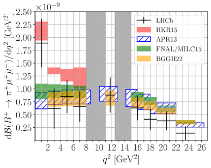
Figure 1: Measured branching fraction of $B^{+}\to\pi^{+}\mu^{+}\mu^{-}$ in bins of dilepton invariant mass squared $q^{2}$ (black points) from LHCb LHCb:2015hsa . SM predictions (this work, BGGH22, yellow) from Tab. 1 are compared to those of Refs. Ali:2013zfa (APR13, blue), Hambrock:2015wka (HKR15, red) and FermilabLattice:2015cdh (FNAL/MILC15, green). Our prediction (yellow) for the last bin is on top of the one from FNAL/MILC15. Plot adapted from LHCb:2015hsa . See text for details.

In the presence of primed NP operators, Eq. 9 can be generalized by

$${C}_{i}^{\text{eff}}(q^{2})\,\to\,{C}_{i}^{\text{eff}}(q^{2})\,+\,C_{i}^{\prime}~{},$$ (11)

noting that due to spin parity of the external states and parity invariance of QCD the Wilson coefficients of unprimed and primed operators enter $B\to\pi\,\ell^{+}\ell^{-}$ decays only by their exact sum, $C_{i^{+}}=C_{i}\,+\,C_{i}^{\prime}$. Taking into account Eq. 11, the binned branching ratios Eq. 10 can be compactly written as

$$\mathcal{B}_{k}^{(B\pi)}\,=\sum_{i=1}^{12}a_{i}^{(B\pi)}\,w_{i}^{(B\pi)}~{},$$ (12)

with the following set of Wilson coefficients combinations

$$w^{(B\pi)}\,=\, \left\{1,\,C_{7^{+}},\,C_{8^{+}},\,C_{9^{+}},\,C_{10^{+}},\,C_{7^{+}}^{2},\,C_{8^{+}}^{2},\,C_{9^{+}}^{2},\right.$$

$$\left.\,C_{10^{+}}^{2},\,C_{7^{+}}\cdot C_{8^{+}},\,C_{7^{+}}\cdot C_{9^{+}},\,C_{8^{+}}\cdot C_{9^{+}}\right\}~{}.$$ (13)

The numerical values of $a^{(B\pi)}_{i}$ for different bins $k$ are given in Tab. 2. Further information regarding uncertainties and correlations is provided in App. A.

II.2.2 $B^{0}_{s}\to\bar{K}^{*0}\mu^{+}\mu^{-}$

The differential branching ratio of $B_{s}^{0}\to\bar{K}^{*0}\mu^{+}\mu^{-}$ decay can be expressed as Ali:1999mm

$$\frac{\text{d}\,\mathcal{B}(B_{s}^{0}\to\bar{K}^{*0}\mu^{+}\mu^{-})}{\text{d}q^{2}}=\mathcal{N}_{B_{s}}\,\lambda_{B_{s}\bar{K}^{*}}^{\frac{3}{2}}\,\mathcal{F}_{B_{s}\bar{K}^{*}}(q^{2})\,,$$ (14)

where the dynamical function $\mathcal{F}_{B_{s}\bar{K}^{*}}(q^{2})$ reads

$$\mathcal{F}_{B_{s}\bar{K}^{*}}(q^{2})=\frac{1}{2}\left(|\mathscr{A}|^{2}+|\mathscr{E}|^{2}\right)\frac{q^{2}}{m_{B_{s}}^{2}}$$

$$+\left(|\mathscr{B}|^{2}+|\mathscr{F}|^{2}\right)\left(\frac{1}{4}\frac{m_{B_{s}}^{2}}{m_{\bar{K}^{*}}^{2}}+3\frac{m_{B_{s}}^{2}q^{2}}{\lambda_{B_{s}\bar{K}^{*}}}\right)$$

$$+\frac{1}{2}\big{(}\text{Re}(\mathscr{B}\,\mathscr{C}^{*})+\text{Re}(\mathscr{F}\,\mathscr{G}^{*})\big{)}\bigg{(}\frac{q^{2}}{m_{\bar{K}^{*}}^{2}}-\frac{m_{B_{s}}^{2}}{m_{\bar{K}^{*}}^{2}}+1\bigg{)}$$

$$+\frac{1}{4}\left(|\mathscr{C}|^{2}+|\mathscr{G}|^{2}\right)\frac{\lambda_{B_{s}\bar{K}^{*}}}{m_{B}^{2}m_{\bar{K}^{*}}^{2}}\,+\,\mathcal{O}\left({m_{\mu}^{2}}\right)~{}.$$ (15)

Here, the functions $\mathscr{A},\,\mathscr{B},...$ contain the dependence on Wilson coefficients and FFs

$$\mathscr{A} =\frac{2}{1+\frac{m_{\bar{K}^{*}}}{m_{B_{s}}}}\,{C}_{9}^{\text{eff}}(q^{2})\,V(q^{2})+\frac{4\,m_{b}}{q^{2}}\,{C}_{7}^{\text{eff}}(q^{2})\,T_{1}(q^{2})~{},$$

$$\mathscr{B} =\left(1+\frac{m_{\bar{K}^{*}}}{m_{B_{s}}}\right)\left[{C}_{9}^{\text{eff}}(q^{2})\,A_{1}(q^{2})\right.$$

$$\left.+\frac{2\,m_{b}}{q^{2}}\left(1-\frac{m_{\bar{K}^{*}}}{m_{B_{s}}}\right){C}_{7}^{\text{eff}}(q^{2})\,T_{2}(q^{2})\right]~{},$$ (16)

$$\mathscr{C} =\left(1-\frac{m_{\bar{K}^{*}}^{2}}{m_{B_{s}}^{2}}\right)^{-1}\left[\left(1-\frac{m_{\bar{K}^{*}}}{m_{B_{s}}}\right){C}_{9}^{\text{eff}}(q^{2})\,A_{2}(q^{2})\right.$$

$$\left.+2\,m_{b}\,{C}_{7}^{\text{eff}}(q^{2})\,\left(T_{3}(q^{2})+\frac{m_{B_{s}}^{2}-m_{\bar{K}^{*}}^{2}}{q^{2}}T_{2}(q^{2})\right)\right]~{},$$

$$\mathscr{E} =2\,\left(1+\frac{m_{\bar{K}^{*}}}{m_{B_{s}}}\right)^{-1}\,{C}_{10}^{\text{eff}}(q^{2})\,V(q^{2})~{},$$

$$\mathscr{F} =\,\left(1+\frac{m_{\bar{K}^{*}}}{m_{B_{s}}}\right)\,{C}_{10}^{\text{eff}}(q^{2})\,A_{1}(q^{2})~{},$$

$$\mathscr{G} =\left(1+\frac{m_{\bar{K}^{*}}}{m_{B_{s}}}\right)^{-1}\,{C}_{10}^{\text{eff}}(q^{2})\,A_{2}(q^{2})~{},$$

where $V(q^{2})$, $A_{0,1,2}(q^{2})$, $T_{1,2,3}(q^{2})$ are the $B_{s}\to\bar{K}^{*}$ transition vector, axial and tensor FFs, respectively. We take them from Ref. Gubernari:2018wyi . As in Eq. 9, we do not show the muon mass corrections. They are given in Ref. Ali:1999mm , and are included in our analysis. Integrating Eq. 14 over $[q^{2}_{\text{min}},q^{2}_{\text{max}}]=[0.1,19]\,\text{GeV}^{2}$, we find

$$\begin{split}\mathcal{B}(B_{s}^{0}\to\bar{K}^{*0}\mu^{+}\mu^{-})_{\text{SM}}=(46.0\pm 6.0)&\cdot 10^{-9}\\ =(46.0\pm 2.1\pm 2.8\pm 3.3\pm 3.6)&\cdot 10^{-9}\,,\end{split}$$ (17)

in agreement with the first experimental evidence from LHCb LHCb:2018rym ,

$$\mathcal{B}(B_{s}^{0}\to\bar{K}^{*0}\mu^{+}\mu^{-})_{\text{exp}}=(29\pm 11)\cdot 10^{-9}\,.$$ (18)

Equation 17 highlights the four main sources of uncertainty: FFs, CKM elements, the renormalization scale $\mu_{b}$, and the effect of the $J/\psi$ and $\psi^{\prime}$ resonances, respectively. The last uncertainty arises from the interpretation of LHCb data LHCb:2018rym which encompasses the resonance regions. In App. B, we provide details on the estimation of the last uncertainty, see Eq. 68.

When chirality-flipped NP effects are turned on, thanks to Lorentz invariance and parity conservation of QCD, they enter either as a sum or difference with the unprimed coefficients, $C_{i^{\pm}}=C_{i}\,\pm\,C_{i}^{\prime}$. Section II.2.2 can therefor be easily adapted through the following replacements in Sec. II.2.2:

$$\begin{split}{C}_{i}^{\text{eff}}(q^{2})\,V(q^{2})&\to\,({C}_{i}^{\text{eff}}(q^{2})\,+C_{i}^{\prime})\,V(q^{2})~{},\\ {C}_{i}^{\text{eff}}(q^{2})\,A_{0,1,2}(q^{2})&\to\,({C}_{i}^{\text{eff}}(q^{2})\,-C_{i}^{\prime})\,A_{0,1,2}(q^{2})~{},\\ {C}_{i}^{\text{eff}}(q^{2})\,T_{1}(q^{2})&\to\,({C}_{i}^{\text{eff}}(q^{2})\,+C_{i}^{\prime})\,T_{1}(q^{2})~{},\\ {C}_{i}^{\text{eff}}(q^{2})\,T_{2,3}(q^{2})&\to\,({C}_{i}^{\text{eff}}(q^{2})\,-C_{i}^{\prime})\,T_{2,3}(q^{2})~{},\end{split}$$ (19)

which result in

$$\mathcal{B}(B_{s}^{0}\to\bar{K}^{*0}\mu^{+}\mu^{-})\,=\sum_{i=1}^{33}\,a^{(B_{s}\bar{K}^{*})}_{i}\,w^{(B_{s}\bar{K}^{*})}_{i}~{},$$ (20)

with

$$w^{(B_{s}\bar{K}^{*})}_{i}\,=\, \left\{1,\,C_{7},\,C_{8},\,C_{9},\,C_{10},\,C_{7}^{2},\,C_{8}^{2},\,C_{9}^{2},\,C_{10}^{2},\right.$$

$$\left.\,C_{7}^{\prime},\,C_{8}^{\prime},\,C_{9}^{\prime},\,C_{10}^{\prime},\,(C_{7}^{\prime})^{2},\,(C_{8}^{\prime})^{2},\,(C_{9}^{\prime})^{2},\right.$$

$$\left.\,(C_{10}^{\prime})^{2},\,C_{7}\cdot C_{7}^{\prime},\,C_{8}\cdot C_{8}^{\prime},\,C_{9}\cdot C_{9}^{\prime},\,C_{10}\cdot C_{10}^{\prime},\right.$$

$$\left.\,C_{7}\cdot C_{8},\,C_{7}^{\prime}\cdot C_{8},\,C_{7}\cdot C_{8}^{\prime},\,C_{7}^{\prime}\cdot C_{8}^{\prime}\right.$$

$$\left.\,C_{7}\cdot C_{9},\,C_{7}^{\prime}\cdot C_{9},\,C_{7}\cdot C_{9}^{\prime},\,C_{7}^{\prime}\cdot C_{9}^{\prime}\right.$$

$$\left.\,C_{8}\cdot C_{9},\,C_{8}^{\prime}\cdot C_{9},\,C_{8}\cdot C_{9}^{\prime},\,C_{8}^{\prime}\cdot C_{9}^{\prime}\right\}\,.$$ (21)

The values of $a^{(B_{s}\bar{K}^{*})}_{i}$ for the $q^{2}$-region $[0.1,\,19]\,\text{GeV}^{2}$ are given in Tab. 3. Information about the uncertainty and correlations is compiled in App. A.

$a^{(B_{s}\bar{K}^{*})}_{1}$	$a^{(B_{s}\bar{K}^{*})}_{2}$	$a^{(B_{s}\bar{K}^{*})}_{3}$	$a^{(B_{s}\bar{K}^{*})}_{4}$	$a^{(B_{s}\bar{K}^{*})}_{5}$	$a^{(B_{s}\bar{K}^{*})}_{6}$	$a^{(B_{s}\bar{K}^{*})}_{7}$	$a^{(B_{s}\bar{K}^{*})}_{8}$	$a^{(B_{s}\bar{K}^{*})}_{9}$	$a^{(B_{s}\bar{K}^{*})}_{10}$	$a^{(B_{s}\bar{K}^{*})}_{11}$
45.96	7.81	0.61	9.51	-12.21	47.92	0.18	1.45	1.44	-15.85	-0.95
$a^{(B_{s}\bar{K}^{*})}_{12}$	$a^{(B_{s}\bar{K}^{*})}_{13}$	$a^{(B_{s}\bar{K}^{*})}_{14}$	$a^{(B_{s}\bar{K}^{*})}_{15}$	$a^{(B_{s}\bar{K}^{*})}_{16}$	$a^{(B_{s}\bar{K}^{*})}_{17}$	$a^{(B_{s}\bar{K}^{*})}_{18}$	$a^{(B_{s}\bar{K}^{*})}_{19}$	$a^{(B_{s}\bar{K}^{*})}_{20}$	$a^{(B_{s}\bar{K}^{*})}_{21}$	$a^{(B_{s}\bar{K}^{*})}_{22}$
-7.52	8.55	47.92	0.18	1.45	1.44	-9.18	-0.05	-2.02	-2.02	3.67
$a^{(B_{s}\bar{K}^{*})}_{23}$	$a^{(B_{s}\bar{K}^{*})}_{24}$	$a^{(B_{s}\bar{K}^{*})}_{25}$	$a^{(B_{s}\bar{K}^{*})}_{26}$	$a^{(B_{s}\bar{K}^{*})}_{27}$	$a^{(B_{s}\bar{K}^{*})}_{28}$	$a^{(B_{s}\bar{K}^{*})}_{29}$	$a^{(B_{s}\bar{K}^{*})}_{30}$	$a^{(B_{s}\bar{K}^{*})}_{31}$	$a^{(B_{s}\bar{K}^{*})}_{32}$	$a^{(B_{s}\bar{K}^{*})}_{33}$
-0.51	-0.51	3.67	9.55	-4.27	-4.27	9.55	0.44	-0.24	-0.24	0.44

Table 3: Central values of $a_{i}^{(B_{s}\bar{K}^{*})}$ in units of $10^{-9}$ for the $q^{2}$-region $[0.1,\,19]$ GeV², see Eq. 20. Further details about uncertainties and correlations are provided in App. A.

II.2.3 $B^{0}\to\mu^{+}\mu^{-}$ and scalar operators

The $B^{0}\to\mu^{+}\mu^{-}$ decay is a clean observable to probe beyond standard model (BSM) physics in $b\to d\,\mu^{+}\mu^{-}$ transitions. In the SM, only the operator $\mathcal{O}_{10}$ contributes which yields Beneke:2019slt including updated CKM values ParticleDataGroup:2022pth

$$\mathcal{B}(B^{0}\to\mu^{+}\mu^{-})_{\text{SM}}\,=\,(1.01\pm 0.07)\cdot 10^{-10}\,,$$ (22)

in agreement with the experimental value LHCb:2021awg

$$\mathcal{B}(B^{0}\to\mu^{+}\mu^{-})_{\text{exp}}=(1.20\pm 0.84)\cdot 10^{-10}\,.$$ (23)

Combining Eqs. 22 and 23, we obtain

$$\frac{\mathcal{B}(B^{0}\to\mu^{+}\mu^{-})_{\text{exp}}}{\mathcal{B}(B^{0}\to\mu^{+}\mu^{-})_{\text{SM}}}\,=\,1.19\pm 0.84~{}.$$ (24)

The purely leptonic decay $B^{0}\to\mu^{+}\mu^{-}$ is sensitive to $\mathcal{O}_{10}^{(\prime)}$, and scalar and pseudoscalar operators,

$$\begin{split}\mathcal{O}_{S}^{(\prime)}\,&=\,(\bar{d}_{L(R)}b_{R(L)})\,(\bar{\mu}\mu)~{},\\ \mathcal{O}_{P}^{(\prime)}\,&=\,(\bar{d}_{L(R)}b_{R(L)})\,(\bar{\mu}\gamma_{5}\mu)~{}.\end{split}$$ (25)

Including their effects, the branching ratio can be written as DeBruyn:2012wk

$$\frac{\mathcal{B}(B^{0}\to\mu^{+}\mu^{-})_{\phantom{\text{SM}}}}{\mathcal{B}(B^{0}\to\mu^{+}\mu^{-})_{\text{SM}}}=\left|\mathcal{P}\right|^{2}+|\mathcal{S}|^{2},$$ (26)

where

$$\mathcal{P} =\frac{C_{10}^{\text{SM}}+C_{10^{-}}}{C_{10}^{\text{SM}}}\,+\,\frac{m_{B}^{2}}{2\,m_{\mu}}\,\left(\frac{1}{m_{b}+m_{d}}\right)\,\left(\frac{C_{P^{-}}}{C_{10}^{\text{SM}}}\right)~{},$$

$$\mathcal{S} =\frac{m_{B}^{2}}{2\,m_{\mu}}\sqrt{1-{4m_{\mu}^{2}\over m_{B}^{2}}}\,\left(\frac{1}{m_{b}+m_{d}}\right)\,\left(\frac{C_{S^{-}}}{C_{10}^{\text{SM}}}\right)~{}.$$ (27)

Setting $C_{P^{-}}$ and $C_{S^{-}}$ to zero, Eq. 24 implies the following ranges for $C_{10^{-}}$:

$$-1.8\lesssim C_{10^{-}}\lesssim 1.7\quad\text{or}\quad 6.7\lesssim C_{10^{-}}\lesssim 10.1~{},$$ (28)

indicating a solution in which NP is a correction to the SM (the first range), and one that involves large cancellations with the SM (the second one), around $C_{10^{-}}$ near $-2\,{C_{10}^{\text{SM}}}$. Future projections for the $300\,\text{fb}^{-1}$ LHC allow for a reduction of uncertainty by a factor $\sim 6$ DiCanto:2022icc . Assuming SM central values, this would lead to improved constraints

$$-0.3\lesssim C_{10^{-}}\!\lesssim 0.3~{}\text{or}~{}8.1\lesssim C_{10^{-}}\!\lesssim 8.6\,(\text{HL-LHC}).$$ (29)

NP effects from scalar and pseudoscalar operators (25) are more strongly constrained by data (24) than $\mathcal{O}_{10}^{(\prime)}$ due to the $m_{B}/m_{\mu}$ factor, leading to

$$-0.06\lesssim C_{P^{-}}\lesssim 0.05\quad\text{or}\quad 0.2\lesssim C_{P^{-}}\lesssim 0.3~{},$$ (30)

$$\hskip 85.35826pt|C_{S^{-}}|\lesssim 0.1\,,$$ (31)

assuming a single NP coefficient at a time. In this work, we do not consider scalar and pseudoscalar contributions in the global fits, and the $B^{0}\to\mu^{+}\mu^{-}$ branching ratio hence depends only on one combination of Wilson coefficients, $C_{10}^{\text{SM}}+C_{10^{-}}$. A decomposition of the branching ratio along the lines of Sec. II.2.1 would result formally in three structures, $\left\{1,C_{10^{-}},C_{10^{-}}^{2}\right\}$, however, all three pre-factors are related, so there is just one coefficient to be varied in the fit.

II.2.4 $b\to d\,\gamma$

The branching ratio of the inclusive decay $\bar{B}\to X_{d}\,\gamma$ can be written as Hurth:2003dk ; Crivellin:2011ba

$$\mathcal{B}(\bar{B}\to X_{d}\gamma)\,=\,\mathcal{N}\left|\frac{V_{td}^{*}V_{tb}}{V_{cb}}\right|^{2}(N+P+P^{\prime})~{},$$ (32)

where the numerical prefactor $\mathcal{N}=(25.7\pm 1.6)\cdot 10^{-4}$ is taken from Ref. Hurth:2003dk . The factor $N=(3.6\pm 0.6)\cdot 10^{-3}$ encodes non-perturbative corrections Gambino:2001ew , whereas $P$ contains the perturbative SM contributions and the NP effects from $\mathcal{O}_{7,8}$, and $P^{\prime}$ accounts for NP contributions from $\mathcal{O}_{7,8}^{\prime}$ operators.

We updated the SM prediction for the CP-averaged $\bar{B}\to X_{d}\,\gamma$ branching ratio

$$\mathcal{B}(\bar{B}\to X_{d}\,\gamma)_{\text{SM}} =(16.8\pm 1.7)\cdot 10^{-6}\,,$$ (33)

from Ref. Misiak:2015xwa . The main improvement is driven by the updated CKM prefactor $\left|(V_{td}^{*}V_{tb})/V_{cb}\right|^{2}\,=\,(41.9\pm 2.5)\cdot 10^{-3}$ ParticleDataGroup:2022pth in Eq. 32. We observe a very good agreement between the SM prediction in Eq. 33 and the extrapolated experimental value from BaBar Misiak:2015xwa ; BaBar:2010vgu ,

$$\mathcal{B}(\bar{B}\to X_{d}\,\gamma)_{\text{exp}}=\left(14.1\pm 5.7\right)\cdot 10^{-6}\,.$$ (34)

Including NP effects from $C_{7,8}^{(\prime)}$ using Ref. Hurth:2003dk , we find the following parametrization

$$\begin{split}\mathcal{B}(\bar{B}\to X_{d}\,\gamma)&=\sum_{i=1}^{9}a^{(\bar{B}X_{d})}_{i}\,w^{(\bar{B}X_{d})}_{i}~{},\end{split}$$ (35)

with

$$w^{(\bar{B}X_{d})}_{i}\,=\, \left\{1,\,C_{7},\,C_{8},\,C_{7}^{2},\,C_{8}^{2},\,\right.$$

$$\left.(C_{7}^{\prime})^{2},\,(C_{8}^{\prime})^{2},\,C_{7}\cdot C_{8},\,C_{7}^{\prime}\cdot C_{8}^{\prime}\right\}\,.$$ (36)

The central values of the factors $a^{(\bar{B}X_{d})}_{i}$ are compiled in Tab. 4. These factors suffer from four sources of uncertainties: renormalization scheme dependence of the ratio $m_{c}/m_{b}$ ($\sim\,$13 %), parametric uncertainties ($\sim\,$7 %), and the perturbative scale $\mu_{b}$ ($\sim\,$4 %), which have been included in our analysis.

$a_{1}^{(\bar{B}X_{d})}$	$a_{2}^{(\bar{B}X_{d})}$	$a_{3}^{(\bar{B}X_{d})}$
$\phantom{-}1.77$	$-6.17$	$-0.28$
$a_{4}^{(\bar{B}X_{d})}=a_{6}^{(\bar{B}X_{d})}$	$a_{5}^{(\bar{B}X_{d})}=a_{7}^{(\bar{B}X_{d})}$	$a_{8}^{(\bar{B}X_{d})}=a_{9}^{(\bar{B}X_{d})}$
$\phantom{-}7.66$	$\phantom{-}0.28$	$\phantom{-}0.53$

Table 4: Central values of $a_{i}^{(\bar{B}X_{d})}$ in units of $10^{-5}$, see Eq. 35.

Experimental information on the exclusive radiative decay $B\to\rho\,\gamma$ is available ParticleDataGroup:2022pth

$$\mathcal{B}(B^{0}\to\rho\,\gamma)_{\text{exp}}\,=\,(8.6\pm 1.5)\cdot 10^{-7}~{},$$ (37)

however its SM prediction

$$\mathcal{B}(B^{0}\to\rho\,\gamma)_{\text{SM}}\,\simeq\,(1.0\pm 1.0)\cdot 10^{-6}~{},$$ (38)

has sizable uncertainties from the tensor FF $T_{1}(0)$. Here, we used $T_{1}^{B\to\rho}(0)\,=\,0.24\pm 0.12$ Gubernari:2018wyi , see therein for earlier LCSR computations, which are consistent but have smaller uncertainties. Confronting the SM to data one obtains the upper limits $\sqrt{|C_{7}^{\text{eff}}|^{2}+|C_{7}^{\prime}|^{2}}\lesssim 0.5\,(0.3)$ at 90 % C.L. from $B\to\rho\gamma\,(B\to X_{d}\gamma)$ branching ratios. Since the dependence on the coefficients is the same up to higher order contributions and non-perturbative effects in the global fit we only take the inclusive modes which gives stronger constraints into account. Once the form factor $B\to\rho$ is more accurately known the exclusive decays give stronger constraints as the measurement is more precise.

III Global $b\to d$ Fits

We perform one-dimensional (1D), two-dimensional (2D) and four-dimensional (4D) fits to various combinations and subsets of the BSM-sensitive Wilson coefficients $C_{7}^{(\prime)},C_{8}^{(\prime)},C_{9}^{(\prime)}$ and $C_{10}^{(\prime)}$ in $|\Delta b|=|\Delta d|=1$ transitions. The fit method is described in Sec. III.1. In Sec. III.2, the set-up of the analysis and the results of the global $b\to d$ fits are presented. A comparison of our limits on semileptonic four-fermion operators with Drell-Yan and dineutrino constraints is presented in Sec. III.3.

The aim of performing higher dimensional fits is in particular to work out and demonstrate the impact and benefits of correlations between different observables and, for the case of the 4D fit, obtain conservative limits for global SMEFT analyses involving semileptonic four-fermion operators.

III.1 Fit method

Using the experimental information from $b\to d$ transitions presented in Sec. II.2, we perform global fits to obtain information on the Wilson coefficients $C_{i}^{(\prime)}$ (collectively denoted here as $\theta$). We work within a frequentist framework based on the approximation of Gaussian likelihood $\mathcal{L}(\theta)=\text{e}^{-\chi^{2}(\theta)/2}$, resulting in the following $\chi^{2}$ function

$$\chi^{2}(\theta)\,=\,-\,2\,\text{ln}\,\mathcal{L}(\theta)\,=\sum_{i,j}^{n_{\text{obs}}}\Delta_{i}(\theta)\,V_{ij}^{-1}(\theta)\,\Delta_{j}(\theta)~{},$$ (39)

with

$$\Delta_{i}(\theta)\, =\,\Delta_{i}^{(\text{th})}(\theta)-\Delta_{i}^{(\text{exp})}~{},$$ (40)

$$V_{ij}(\theta)\, =\,V^{(\text{th})}_{ij}(\theta)+V^{(\text{exp})}_{ij}~{}.$$ (41)

Here, $n_{\text{obs}}$ represents the number of observables included in the fit ($n_{\text{obs}}=6$), with

$$\vec{\Delta}\,=\,\{ \mathcal{B}_{1}^{(B\pi)},\mathcal{B}_{2}^{(B\pi)},\mathcal{B}_{9}^{(B\pi)},\mathcal{B}(B_{s}^{0}\to\bar{K}^{*0}\mu^{+}\mu^{-}),$$

$$\mathcal{B}(B^{0}\to\mu^{+}\mu^{-}),\mathcal{B}(\bar{B}\to X_{d}\,\gamma)\}\,.$$ (42)

Furthermore, $\Delta_{i}^{(\text{th})}(\theta)$ is the central value of the theory prediction for the $i$-th observable, $\Delta_{i}^{(\text{exp})}$ is the central value of the experimental measurement of the same observable, while $V^{(\text{th})}_{ij}(\theta)$ and $V^{(\text{exp})}_{ij}$ are the theoretical and experimental covariance matrices, respectively. We provide details on the computation of these matrices in App. A. To estimate the central values of the $\theta$ parameters, we use the maximum likelihood (ML) method. By construction of $\mathcal{L}(\theta)$, the ML estimators $\hat{\theta}$ correspond to the best-fit points obtained by minimizing the $\chi^{2}(\theta)$ function, that is $\partial\,\chi^{2}/\partial\,\theta_{i}|_{\hat{\theta}}=0$ with $i=1,...,n_{\text{par}}$ and $n_{\text{par}}$ being the number of parameters (up to 8 parameters in the most general scenario). In practise, we use MIGRAD from the Python package iminuit hans_dembinski_2022_6330776 to conduct the numerical minimization. We scan for the viable parametric space of $\theta$ by initializing the MIGRAD algorithm to different initial values of $\theta$. In some cases, we find multiple solutions with similar $\chi^{2}_{\text{min}}\equiv\chi^{2}(\hat{\theta})$, we always choose the one with a smaller $\chi^{2}$ value. In that sense, future measurements of $b\to d\,\,\mu^{+}\mu^{-}$ modes are necessary to exclude other solutions with larger $\chi^{2}$ values.

The confidence regions for $l=1,2,...$ sigmas are worked out via $\Delta\chi^{2}(\theta)\leq\eta\,(l,n_{\text{par}})$ where $\Delta\chi^{2}(\theta)=\chi^{2}(\theta)-\chi^{2}_{\text{min}}$ and $\eta\,(l,n_{\text{par}})$ is the value where the $\chi^{2}$ cumulative distribution (CDF) function reaches the probability associated with $l$ sigmas, e.g. $\eta\,(l,1)=l^{2}$, $\eta\,(l,2)=(2.30,6.18,...)$, etc. In practise, the confidence intervals are computed using MINOS algorithm from iminuit hans_dembinski_2022_6330776 .

With the explicit dependence of the $\chi^{2}$ function given by Eq. 39, we compute the errors, $\sigma_{\hat{\theta}_{i}}=\sqrt{(V_{\hat{\theta}})_{ii}}$, and the correlations among the fit parameters, $\rho_{\hat{\theta}_{i}\hat{\theta}_{j}}\equiv(V_{\hat{\theta}})_{ij}/\sqrt{(V_{\hat{\theta}})_{ii}(V_{\hat{\theta}})_{jj}}$, which are given by the matrix

$$(V_{\hat{\theta}}^{-1})_{ij}\,=\,\left.\frac{1}{2}\frac{\partial^{2}\chi^{2}}{\partial\theta_{i}\partial\theta_{j}}\right|_{\hat{\theta}}~{}.$$ (43)

These matrices are provided as an output by MIGRAD when performing the minimization routine.

To determine the level of statistical significance between a given hypothesis $H$ and the data, we also determine the $p-$value of the respective fit,

$$p_{H}=1-\text{CDF}(\chi^{2}_{\text{min}};n_{\text{dof}})~{},$$ (44)

where $n_{\text{dof}}=n_{\text{obs}}-n_{\text{par}}$ is the number of degrees of freedom. A $p-$value of less than 0.05 indicates strong evidence against the assumed hypothesis, as there is less than a 5% probability that $H$ is correct. Finally, to compare the description offered by two hypotheses $H$ and SM, we provide their relative pull (in units of standard deviations $\sigma$)

$$\text{Pull}_{H}\,=\,\sqrt{2}\,\text{Erf}^{-1}\left[\text{CDF}(\Delta\chi^{2}_{H};n_{H})\right]~{},$$ (45)

where Erf is the error function, $\Delta\chi^{2}_{H}=\chi^{2}_{\text{SM},\text{min}}-\chi^{2}_{H,\text{min}}$, and $n_{H}$ is the number of parameters in $H$.

III.2 Results for Wilson coefficient fits

In the following, we present the fit results for 1D, 2D, and 4D scenarios floating different combinations of NP Wilson coefficients. The main results of the fits are given in Tabs. 5, 6, and 7. Constraints on NP Wilson coefficients $C_{i},C_{i}^{\prime}$ are given at the $b$-quark mass scale. The SM hypothesis gives a good fit to $b\to d\,\mu^{+}\mu^{-}$ and $b\to d\,\gamma$ data ($n_{\text{obs}}\,=\,6$), resulting in $\chi^{2}_{\text{min}}\,=\,3.77$ and a $p-$value of 71 %.

scenario	fit parameter	best fit	$1\sigma$	$2\sigma$	$\chi^{2}_{H_{i},\,\text{min}}$	Pull${}_{H_{i}}$	$p$-value (%)
$H_{1}$	$C_{7}$	0.01	[-0.07, 0.11]	[-0.15, 0.25]	3.74	0.15	58
$H_{2}$	$C_{8}$	0.04	[-0.88, 1.44]	[-1.51, 2.27]	3.76	0.04	58
$H_{3}$	$C_{9}$	-1.37	[-2.97, -0.47]	[-7.65, 0.26]	1.12	1.63	95
$H_{4}$	$C_{10}$	0.96	[0.3, 1.75]	[-0.29, 2.92]	1.51	1.50	91
$H_{5}$	$C_{7}^{\prime}$	-0.02	[-0.18, 0.16]	[-0.31, 0.3]	3.75	0.11	58
$H_{6}$	$C_{8}^{\prime}$	-0.04	[-1.16, 1.13]	[-1.86, 1.85]	3.76	0.03	58
$H_{7}$	$C_{9}^{\prime}$	-0.21	[-0.91, 0.47]	[-1.63, 1.15]	3.67	0.32	59
$H_{8}$	$C_{10}^{\prime}$	0.22	[-0.37, 0.8]	[-0.98, 1.38]	3.63	0.37	60
$H_{9}$	$C_{9}=+C_{10}$	0.19	[-0.57, 1.02]	[-1.24, 1.79]	3.71	0.24	59
$H_{10}$	$C_{9}=-C_{10}$	-0.53	[-0.89, -0.19]	[-1.29, 0.14]	1.27	1.58	93
$H_{11}$	$C_{9}^{\prime}=+C_{10}^{\prime}$	0.10	[-0.68, 0.86]	[-1.41, 1.53]	3.75	0.13	58
$H_{12}$	$C_{9}^{\prime}=-C_{10}^{\prime}$	-0.13	[-0.46, 0.22]	[-0.8, 0.57]	3.63	0.37	60
$H_{13}$	$C_{9}=-C_{9}^{\prime}$	-1.74	[-3.26, -0.27]	[-4.04, 0.44]	1.96	1.34	85
$H_{14}$	$C_{9}=+C_{9}^{\prime}$	-0.55	[-1.29, -0.07]	[-4.13, 0.34]	2.42	1.16	78
$H_{15}$	$C_{9}=-C_{10}=-C_{9}^{\prime}=-C_{10}^{\prime}$	-0.58	[-1.06, -0.2]	[-4.04, 0.12]	1.17	1.61	94
$H_{16}$	$C_{9}=-C_{10}=+C_{9}^{\prime}=-C_{10}^{\prime}$	-0.24	[-0.46, -0.04]	[-0.7, 0.16]	2.35	1.19	79

Table 5: Fit results for Wilson coefficients in the 1D scenarios ($H_{1,...,16}$) at the scale $\mu_{b}$. Best-fit values and $1\sigma$ ($2\sigma$) uncertainties are displayed in the third and fourth (fifth) columns. The indicators of the goodness-of-fit are provided in the last columns: $\chi^{2}$ function evaluated at the best-fit point; the Pull${}_{H_{i}}$ in units of standard deviation, as in Eq. 45; and the $p-$value $p_{H}$, as in Eq. 44. The SM has $\chi^{2}_{\text{SM}}=3.77$, with a $p-$value of 71%.

III.2.1 One-dimensional fits

We start with 1D scenarios ($H_{1,...,16}$), which are compiled in Tab. 5. Here, the first column displays the name of the scenario, while the second column indicates the fitted Wilson coefficient and the correlations assumed between other Wilson coefficients, as in $H_{9,...,16}$. The best-fit values with their 1$\sigma$ and 2$\sigma$ confidence intervals are given in the third and fourth columns, respectively. The last columns show the indicators of the goodness-of-fit: best-fit $\chi^{2}$ value, the pull from the SM hypothesis, see Eq. 45, and the $p-$value of the fit, see Eq. 44.

Among the 1D scenarios with only one Wilson coefficient switched on at a time, $H_{1,...,8}$, the most favored one is $H_{3}$ with NP in $C_{9}$ only, with a pull of $1.63\,\sigma$ and a $p-$value of 95%. The second most favored scenario is $H_{4}$ with a pull of $1.50\,\sigma$ and a $p-$value of 91%, where NP only enters in $C_{10}$. One observes that the global fit selects the solution with the smaller NP effect from the ranges given by $B^{0}\to\mu^{+}\mu^{-}$ alone, see Eq. 28.

scen.	fit parameters	best fit	$1\sigma$	$2\sigma$	$\chi^{2}_{H_{i},\,\text{min}}$	Pull${}_{H_{i}}$	$p$-v. (%)
$H_{17}$	($C_{7}$, $C_{8}$)	(0.02, -0.13)	([-0.08, 0.21], [-1.57, 1.46])	([-0.16, 0.43], [-2.37, 2.41])	3.74	0.02	44
$H_{18}$	($C_{7}$, $C_{9}$)	(0.05, -1.45)	([-0.04, 0.19], [-3.0, -0.54])	([-0.13, 0.94], [-9.65, 0.22])	0.86	1.19	93
$H_{19}$	($C_{7}$, $C_{10}$)	(0.04, 1.02)	([-0.05, 0.17], [0.34, 1.87])	([-0.13, 0.73], [-0.26, 3.32])	1.33	1.05	85
$H_{20}$	($C_{7}$, $C_{7}^{\prime}$)	(0.01, -0.02)	([-0.07, 0.12], [-0.21, 0.17])	([-0.15, 0.28], [-0.36, 0.34])	3.73	0.02	44
$H_{21}$	($C_{7}$, $C_{9}^{\prime}$)	(0.02, -0.23)	([-0.07, 0.12], [-0.92, 0.46])	([-0.15, 0.26], [-1.64, 1.15])	3.63	0.08	45
$H_{22}$	($C_{7}$, $C_{10}^{\prime}$)	(0.02, 0.23)	([-0.07, 0.12], [-0.36, 0.81])	([-0.15, 0.26], [-0.97, 1.4])	3.60	0.10	46
$H_{23}$	($C_{9}$, $C_{10}$)	(-1.67, 8.55)	([-7.43, 0.65], [6.48, 9.37])	([-9.13, 1.86], [-1.42, 9.85])	1.00	1.15	91
$H_{24}$	($C_{7}^{\prime}$, $C_{9}$)	(0.05, -1.4)	([-0.17, 0.23], [-2.95, -0.49])	([-0.35, 0.36], [-7.64, 0.26])	1.08	1.12	89
$H_{25}$	($C_{9}$, $C_{9}^{\prime}$)	(-2.22, 1.18)	([-6.55, -0.63], [-2.99, 2.89])	([-7.58, 0.23], [-3.92, 3.81])	0.76	1.22	94
$H_{26}$	($C_{9}$, $C_{10}^{\prime}$)	(-1.79, -0.35)	([-6.59, -0.57], [-1.19, 0.36])	([-7.61, 0.27], [-1.8, 1.05])	0.88	1.18	92
$H_{27}$	($C_{7}^{\prime}$, $C_{10}$)	(0.04, 0.99)	([-0.16, 0.22], [0.31, 1.84])	([-0.3, 0.35], [-0.29, 3.25])	1.48	1.00	83
$H_{28}$	($C_{9}^{\prime}$, $C_{10}$)	(0.21, 7.34)	([-0.58, 0.99], [6.29, 8.09])	([-1.39, 1.79], [-0.3, 8.72])	1.35	1.04	85
$H_{29}$	($C_{10}$, $C_{10}^{\prime}$)	(7.45, -0.01)	([6.53, 8.13], [-0.79, 0.97])	([-0.30, 8.73], [-4.54, 4.49])	1.42	1.02	84
$H_{30}$	($C_{7}^{\prime}$, $C_{9}^{\prime}$)	(0.02, -0.26)	([-0.18, 0.21], [-1.07, 0.57])	([-0.32, 0.34], [-1.88, 1.36])	3.66	0.07	45
$H_{31}$	($C_{7}^{\prime}$, $C_{10}^{\prime}$)	(0.0, 0.22)	([-0.17, 0.18], [-0.41, 0.84])	([-0.31, 0.32], [-1.04, 1.46])	3.63	0.08	45
$H_{32}$	($C_{9}^{\prime}$, $C_{10}^{\prime}$)	(-0.08, 0.17)	([-1.07, 0.83], [-0.65, 0.99])	([-2.04, 1.63], [-1.39, 1.74])	3.62	0.09	45
$H_{33}$	$(C_{9}=-C_{9}^{\prime},\,C_{10}=+C_{10}^{\prime})$	(-1.73, 0.44)	([-3.34, -0.19], [0.04, 0.95])	([-4.1, 0.51], [-0.34, 4.52])	0.77	1.22	94
$H_{34}$	$(C_{9}=-C_{9}^{\prime},\,C_{10}=-C_{10}^{\prime})$	(-1.73, 0.01)	([-3.65, 0.15], [-0.45, 0.91])	([-4.6, 1.05], [-0.84, 5.06])	1.96	0.83	74
$H_{35}$	$(C_{9}=+C_{9}^{\prime},\,C_{10}=+C_{10}^{\prime})$	(0.6, 2.18)	([0.26, 0.89], [-0.58, 4.77])	([-4.95, 1.19], [-0.92, 5.1])	2.15	0.76	70
$H_{36}$	$(C_{9}=-C_{10},\,C_{9}^{\prime}=+C_{10}^{\prime})$	(-0.58, 0.57)	([-3.11, -0.2], [-1.37, 3.38])	([-8.03, 0.13], [-3.14, 4.05])	1.17	1.10	88
$H_{37}$	$(C_{9}=-C_{10},\,C_{9}^{\prime}=-C_{10}^{\prime})$	(-0.6, 0.15)	([-1.07, -0.21], [-0.27, 0.65])	([-1.86, 0.15], [-0.66, 1.47])	1.15	1.10	88

Table 6: Fit results for the 2D scenarios with similar description as Tab. 5.

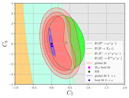
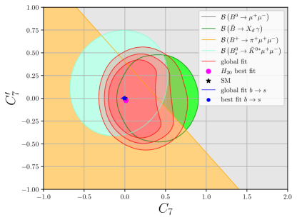
Figure 2: Results of the 2D fits to Wilson coefficients $C_{7}$,$C_{8}$ (scenario $H_{17}$, left panel) and $C_{7}$,$C_{7}^{\prime}$ (scenario $H_{20}$, right panel), see Tab. 6. We show the 1$\sigma$ allowed regions of the individual observables and the combined 1, 2, and $3\sigma$ regions (red). The black star at the origin represents the SM. Results of the global $b\to s$ fit, see App. C, are superimposed (blue) and serve as a data-driven prediction assuming minimal flavor violation (MFV). Deviations between the blue area and the SM are a result of the present discrepancies in $b\to s$ processes with the SM. See text for details.

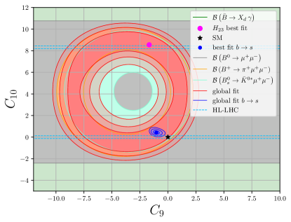
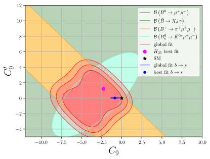
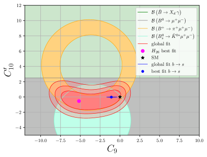
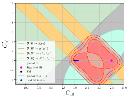
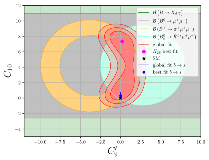
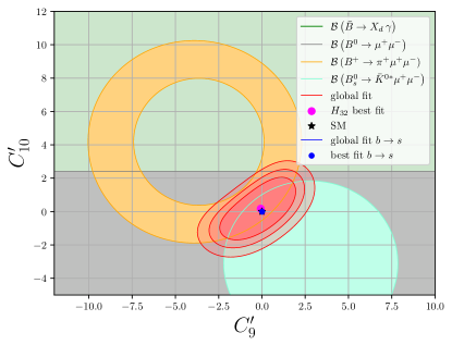
Figure 3: Results of the 2D fits to semileptonic four-fermion operators, see Tab. 6. Similar description as in Fig. 2.

Furthermore, we perform global fits in scenarios relating two Wilson coefficients ($H_{9,...,14}$) in which $SU(2)_{L}$-invariance is preserved in the lepton sector or those with a preference for leptonic vector-couplings. We find that the scenario $H_{10}$ with left-handed quarks and left-handed leptons, $C_{9}=-C_{10}$, is preferred by data with a pull of $1.58\,\sigma$ and a $p-$value 93%. For comparison, benchmark $H_{9}$, that is, left-handed quarks and right-handed leptons $C_{9}=C_{10}$, only has a pull of $0.24\,\sigma$ and a $p-$value 59%, worse than the SM one. These findings are similar to the ones in $b\to s$ transitions where a good fit is obtained for $C_{9}^{(b\to s)}=-C_{10}^{(b\to s)}=-0.50\pm 0.13$, see App. C. We explore additional correlations among the primed coefficients $C_{9,10}^{\prime}$ exploiting $C_{9}^{\prime}=\pm\,C_{10}^{\prime}$, see scenarios $H_{11}$ and $H_{12}$ with $p-$values worse than the SM one. In addition, we consider $C_{9}=\pm\,C_{9}^{\prime}$, which gives a pull of $1.34\,\sigma$ and a $p-$value of 85% for $C_{9}=-C_{9}^{\prime}$, while a $p$-value of $78\,$% is obtained for $C_{9}=+C_{9}^{\prime}$. Taking into account the previous observations, we perform a fit in scenarios involving four NP coefficients, $H_{15}$ and $H_{16}$, where the most preferred scenario is $H_{15}$ with a pull of $1.61\,\sigma$ and a $p-$value 94%.

We observe that data shows a clear preference to include NP via $C_{9}$, following a similar pattern as in global fits to $b\to s\,\mu^{+}\mu^{-}$ data, where $C_{9}^{(b\to s)}=-0.85\pm 0.21$ gives a good fit, see App. C. Therefore, future data is very welcome to confirm or refute this pattern in other flavor sectors, such as $b\to d$ transitions.

To summarize, while there is consistency with the SM, we also observe room for sizable, order one NP contributions to Wilson coefficients, significantly larger than corresponding ranges in the $b\to s$ global fit. We note also that the likelihood is quite flat, making uncertainty ranges more sensible than best-fit points. These features continue to hold in 2D and 4D fits discussed next.

III.2.2 Two-dimensional fits

Here we present the results for the 2D fits which are compiled in Tab. 6. We exploit scenarios composed out of two coefficients from $C_{7},C_{7}^{\prime},C_{8},C_{9},C_{9}^{\prime},C_{10},C_{10}^{\prime}$ in $H_{17,...,32}$. The presently most favored scenario is $H_{25}$ with a pull of $1.22\,\sigma$ and a $p-$value of 94%, fitting simultaneously $C_{9}$ and $C_{9}^{\prime}$. We observe again a similar pattern as in the 1D fits, that, if $C_{9}$ is included in the fit, $p-$values are large, $\sim 90\%$, i.e. $H_{18,23,24,25,26}$. In addition, we perform fits in scenarios where NP enters in a correlated way in four Wilson coefficients, $H_{33,...,37}$. Among these, scenario $H_{33}$, with $C_{9}=-C_{9}^{\prime}$ and $C_{10}=+C_{10}^{\prime}$, features the highest pull of $1.22\,\sigma$ and a large $p-$value of $94\%$. Some of these benchmark models, $H_{34,35,37}$ satisfy the relation $C_{10}^{\prime}/C_{10}=C_{9}^{\prime}/C_{9}$, which arises from tree-level exchange of a $Z^{\prime}$-boson Descotes-Genon:2015uva .

In Fig. 2, we display two selected 2D contours of scenarios with dipole coefficients, $H_{17}$ ($C_{7}$ and $C_{8}$) and $H_{20}$ ($C_{7}$ and $C_{7}^{\prime}$). One observes an excellent complementarity between $\bar{B}\to X_{d}\gamma$, $B^{+}\to\pi^{+}\mu^{+}\mu^{-}$, and $B^{0}_{s}\to\bar{K}^{0*}\mu^{+}\mu^{-}$ observables. This leads to improved limits on $C_{7}^{(\prime)}$ compared to previous works Crivellin:2011ba (assuming real-valued Wilson coefficients).

scen.	fit parameter	$1\sigma$	$2\sigma$	$\chi^{2}_{H_{i},\,\text{min}}$	Pull${}_{H_{i}}$	$p$-v. $(\%)$
$H_{38}$	($C_{9}$, $C_{9}^{\prime}$, $C_{10}$, $C_{10}^{\prime}$)	([-7.96, 0.84], [-4.42, 4.34], [-0.89, 9.31], [-5.12, 5.08])	([-9.06, 1.83], [-5.45, 5.36], [-1.40, 26.4], [-21.8, 5.59])	0.68	0.61	71
$H_{39}$	($C_{7}$, $C_{8}$, $C_{9}$, $C_{10}$)	([-0.04, 0.85], [-2.29, 2.53], [-9.7, 0.26], [-1.06, 1.97])	([-0.13, 2.09], [-2.74, 2.98], [-11.05, 1.77], [-1.55, 9.94])	0.53	0.65	76

Table 7: Fit results for the 4D scenarios ($H_{38,39}$). Further notation as in Tabs. 5 and 6.

In Fig. 3, we display contours from fits to semileptonic four-fermion operators. We observe that the complementarity between the observables is currently not as good as for dipole coefficients, leading to weaker limits on $C_{9}$ and $C_{10}$, see the uppermost left plot of Fig. 3, displaying contours in $H_{23}$, $C_{9}$ versus $C_{10}$. The branching ratios of $B^{+}\to\pi^{+}\mu^{+}\mu^{-}$, and $B^{0}_{s}\to\bar{K}^{0*}\mu^{+}\mu^{-}$ cooperate to reduce the thickness of the annulus (red area) but do not lift the degeneracy between $C_{9}$ and $C_{10}$. The branching ratio of $B^{0}\to\mu^{+}\mu^{-}$ can in principle do so due to its dependence on $C_{10}^{(\prime)}$ only, however, the present precision is insufficient. In the future, the HL-LHC run can improve this significantly, see Eq. 29 for the projected sensitivity, up to a discrete ambiguity. This is illustrated by the dashed blue horizontal lines in the uppermost left plot of Fig. 3. Note also that due to the flat likelihood along the ring (red area) the best-fit point (magenta) is only shown for completeness but has little statistical preference over other points in this flat direction. The projections in Fig. 3 also make visible discrete ambiguities, for instance the two yellow bands in $C_{10},C_{10}^{\prime}$ (mid right-handed plot).

To remove the ambiguities additional complementary observables of $b\to d\,\ell\ell$ transitions are necessary. As well known from the early days of the $b\to s\,\mu\mu$ fits, angular observables break the degeneracy in the branching ratio based fits and significantly improve the information on the NP couplings Ali:2002jg ; Bobeth:2010wg . The most simple one is the forward-backward asymmetry $A_{\text{FB}}^{\ell}$ in the lepton angle, defined as

$$A_{\text{FB}}^{\ell}\propto\int_{0}^{1}\!\!\text{d}\cos\theta_{\ell}\frac{\text{d}^{2}\Gamma}{\text{d}q^{2}\text{d}\cos\theta_{\ell}}-\int_{-1}^{0}\!\!\text{d}\cos\theta_{\ell}\frac{\text{d}^{2}\Gamma}{\text{d}q^{2}\text{d}\cos\theta_{\ell}}$$ (46)

and $\theta_{\ell}$ is the angle between the negatively charged lepton and the decaying $b$-hadron in the dilepton center of mass system. In $1/2\to 1/2\,\ell^{+}\ell^{-}$ baryon or $0\to 1\,\ell^{+}\ell^{-}$ meson decays, where we indicate the spin of the initial and final hadron, $A_{\text{FB}}^{\ell}$ is sensitive to the product of Wilson coefficients $C_{9}C_{10}$ rather than the sum of squares as the branching ratios. Therefore, in terms of constraints, the latter provide ellipses, while $A_{\text{FB}}^{\ell}$ gives hyperbolas in the $C_{9}$-$C_{10}$ plane Ali:1994bf . Further observables with complementary dependence on the Wilson coefficients arise from full angular analysis.

Already a rough measurement of $A_{\text{FB}}^{\ell}$ can signal new physics, and rule out large classes of BSM models and non-SM flavor structures Ali:1999mm . The Belle collaboration determined the sign of $A_{\text{FB}}^{\ell}$ in $b\to s$ transitions based on $113.6\pm 13$ events of $B\to K^{*}\ell^{+}\ell^{-}$ decays Belle:2006gil . Since LHCb evidenced $\bar{B}_{s}\to\bar{K}^{*0}\mu\mu$ with $38\pm 12$ events LHCb:2018rym , one could expect that this crucial test in the $b\to d$ sector can be performed in the not too far future.

Let us further entertain a comparison with the $b\to s$ global fits. The latter can be related to $b\to d$ processes assuming that quark flavor violation is realized minimally – induced by the known quark masses and mixing angles. Within the weak effective theory (1), this implies universal Wilson coefficients $C_{i}$, allowing them to be compared between the two fits. For the primed coefficients an additional factor of down to strange quark masses is involved, $C_{i}^{\prime\,(b\to d)}=(m_{d}/m_{s})\,C_{i}^{\prime\,(b\to s)}$. A disagreement between the resulting $b\to s$ and $b\to d$ Wilson coefficients would signal additional sources of quark flavor violation beyond the SM. In Figs. 2 and 3, we show in addition to the $b\to d$ results (red) the global fit results for the same scenarios using $b\to s$ input (blue), see App. C. The fact that the SM (black star) is not included in the $b\to s$ preferred regions is a reflection of the present anomalies in this sector.

We observe as expected from the significantly more precise data in the $b\to s$ sector, that the latter is significantly stronger constrained than the $b\to d$ one. Due to the quark mass suppression, $m_{d}/m_{s}\sim 0.1$, the derived constraints on the primed coefficients are even stronger, and result in narrow regions in the corresponding plots. One also notices that the preferred region for $b\to s$ is inside the $b\to d$ one. Data are therefore consistent with the hypothesis of minimal quark flavor violation. To test this further requires improved data on $b\to d$ transitions. The anticipated reach in $B_{d}\to\mu^{+}\mu^{-}$ from the HL-LHC DiCanto:2022icc given in Eq. 29 probes the present MFV prediction in $C_{10}$, see e.g., the upper left plot of Fig. 3. On the other hand, there is a sizable window for flavorful new physics in $b\to d$ modes, and new physics can be just around the corner. Observing for instance a wrong sign $A_{\text{FB}}^{\ell}$ with the next round of data would signal a breakdown of the SM, and of MFV.

III.2.3 Four-dimensional fits

We perform 4D fits (scenarios $H_{38}$ and $H_{39}$), where the numerical results are presented in Tab. 7. Results are consistent with those of the 1D and 2D scenarios, but exhibit larger uncertainties due to the larger number of parameters. This is to be expected as already good fits where obtained for 1D and 2D scenarios, so the additional degrees of freedom are not needed to improve the consistency with the data. For this reason, we do not show contour plots of the 4D fits. On the other hand, the more general situation with four independent couplings describes more general NP models.

III.3 Interplay with $b\to d\,\nu\bar{\nu}$ and high-$p_{T}$

For completeness, we compare our results with the limits extracted using other experimental information. To do so, it is convenient to introduce the following combinations of Wilson coefficients

$$\kappa_{L}^{bd\mu\mu}\,=\,C_{9}-C_{10}~{},~{}~{}\kappa_{R}^{bd\mu\mu}\,=\,C_{9}^{\prime}-C_{10}^{\prime}~{},$$ (47)

which project onto couplings to left-handed leptons. The methodology is based on Bause:2021cna . In Tab. 8, we show the limits on $\kappa_{L(R)}^{bd\mu\mu}$ obtained in the 4D scenario $H_{38}$ $(C_{9},C_{9}^{\prime},C_{10},C_{10}^{\prime})$, which update those from Bause:2021cna by taking into account correlations. Also given are limits using data on rare $B$ decays into dineutrinos Bause:2021cna , as well as high-$p_{T}$ constraints Fuentes-Martin:2020lea ; Angelescu:2020uug . The limits from the global fit obtained in this work are a factor 30 (20) stronger than the limits extracted from dineutrino modes (Drell-Yan processes).

Data	$\kappa_{R}^{bd\mu\mu}$	$\kappa_{L}^{bd\mu\mu}$
Rare $B$ decays to dimuons	$[-7.2,7.2]$	$[-15.0,-0.6]$
Rare $B$ decays to dineutrinos	$210$	$-$
Drell-Yan	$314$	$314$

Table 8: Limits on $\kappa_{R,L}^{bd\mu\mu}$ couplings. The second row gives the $1\sigma$ results from our global $b\to d\,\mu^{+}\mu^{-}$ fit to $C_{9},C_{9}^{\prime},C_{10},C_{10}^{\prime}$ (scenario $H_{38}$). The third row displays the bound on $\kappa_{R}^{bd\mu\mu}$ from dineutrino modes using $SU(2)_{L}$ taken from Ref. Bause:2021cna . The last row displays upper limits extracted from high-$p_{T}$ data, that is, Drell-Yan processes Fuentes-Martin:2020lea ; Angelescu:2020uug .

Applications of the FCNC $|\Delta b|=|\Delta d|=1$ global fits are flavor studies in dineutrino modes Bause:2020auq . Branching ratios of $b\to d\,\nu\bar{\nu}$ decays are related to lepton flavor-specific data using an $SU(2)_{L}$-link, that can be formulated in SMEFT. Constraints on dineutrinos derived from charged dileptons depend on whether lepton universality or charged lepton flavor violation holds, and can hence probe lepton flavor structure. This is demonstrated in Fig. 4, where $\mathcal{B}(B^{0}\to\rho^{0}\nu\bar{\nu})$ versus $\mathcal{B}(B^{0}\to\pi^{0}\nu\bar{\nu})$ is displayed. We show the region consistent with lepton universality at $1\sigma$ (purple area) and $2\sigma$ (purple dashed lines). The SM predictions (blue) Bause:2021cna

$$\begin{split}\mathcal{B}(B^{0}\to\pi^{0}\nu\bar{\nu})_{\text{SM}}&=(5.4\pm 0.6)\cdot 10^{-8},\\ \mathcal{B}(B^{0}\to\rho^{0}\nu\bar{\nu})_{\text{SM}}&=(22\pm 8)\cdot 10^{-8},\end{split}$$ (48)

are well below the experimental limits (gray exclusion areas). The hatched ones are direct upper limits while the unhatched ones are derived from the presently strongest upper limits on the dineutrino modes, ${\mathcal{B}}(B^{+}\to\pi^{+}\nu\bar{\nu})<1.4\cdot 10^{-5}$ and ${\mathcal{B}}(B^{+}\to\rho^{+}\nu\bar{\nu})<3\cdot 10^{-5}$ (at 90% CL) Belle:2017oht . If dineutrino branching ratios are observed in the future outside the purple cones lepton flavor universality is violated.

Figure 4 updates the corresponding plot from Ref. Bause:2021cna by taking into account the somewhat larger range of $\kappa_{R}^{bd\mu\mu}$ due to correlations in the global fit . While the cones predicted assuming universality (purple) are consequently somewhat wider, this is a barely visible effect as the width is fully dominated by FF uncertainties, see Ref. Bause:2021cna for details.

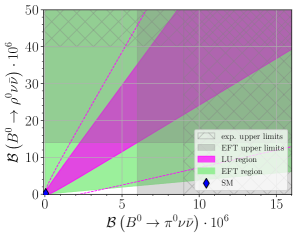
Figure 4: $\mathcal{B}(B^{0}\to\rho^{0}\nu\bar{\nu})$ versus $\mathcal{B}(B^{0}\to\pi^{0}\nu\bar{\nu})$. The region consistent with lepton universality is shown at $1\sigma$ (purple area) and $2\sigma$ (purple dashed lines) using $SU(2)_{L}$ and $\kappa_{R}^{bd\mu\mu}=0.0\pm 7.2$. SM predictions (48) are shown as the blue diamond. The non-green area is outside the effective theory description. Gray regions indicate experimental exclusion limits. See Ref. Bause:2021cna and text for details.

IV Conclusions

We present the first model-independent analysis of rare radiative and semileptonic $|\Delta b|=|\Delta d|=1$ processes based on the branching ratios of $B^{+}\to\pi^{+}\mu^{+}\mu^{-}$, $B^{0}_{s}\to\bar{K}^{*0}\mu^{+}\mu^{-}$, $B^{0}\to\mu^{+}\mu^{-}$, and $B\to X_{d}\gamma$ decays. The detailed numerical outcome of the global fits to Wilson coefficients of dipole $C_{7}^{(\prime)},C_{8}^{(\prime)}$ and four-fermion operators $C_{9}^{(\prime)},C_{10}^{(\prime)}$ is given in Tabs. 5, 6, and 7.

We find that data are consistent with the SM, but also leave sizable room for new physics. Contributions to Wilson coefficients can be order one in $b\to d$ processes, significantly larger than corresponding ranges in the $b\to s$ transitions, as shown in Figs. 2 and 3. The preferred regions of the $b\to d$ Wilson coefficients (red areas), collapse to the smaller, included ones from $b\to s$ fits (blue areas) in models with minimal quark flavor violation, indicating consistency with MFV. To test this paradigm at the level of the current $b\to s$ prediction the $b\to d$ fit needs to be significantly improved. This is within the HL-LHC reach of the $B_{d}\to\mu^{+}\mu^{-}$ branching for the Wilson coefficient $C_{10}$ (29). In the meantime, since flavorful new physics may be just around the corner, it can show up in $b\to d$ angular distributions and could rule out MFV. Note that the pattern of branching ratios suppressed with respect to the SM in $b\to s\,\mu\mu$ decays continues to hold for the $b\to d\,\mu\mu$ ones, although within larger uncertainties, see Figs. 1, 17, and 18.

Due to several flat directions in parameter space but also sizable uncertainties, the likelihood for the semileptonic four-fermion operators is quite flat. Consequently, improving the fit is not just a matter of higher statistics, but also of adding observables sensitive to different combinations of Wilson coefficients than the branching ratios. Such observables are the very well-known leptonic forward-backward asymmetries in semileptonic decays of $b$-mesons or $b$-baryons, see Eq. 46, $B_{s}^{0}\to\bar{K}^{*0}\,\ell^{+}\ell^{-}$, $B\to\rho\,\ell^{+}\ell^{-}$, $\Xi_{b}\to\Sigma\,\ell^{+}\ell^{-}$ or $\Omega_{b}^{-}\to\Xi^{-}\,\ell^{+}\ell^{-}$ or a full angular analysis thereof including secondary hadronic decays. We point out here opportunities from $\Omega_{b}^{-}\to\Xi^{-}\,(\to\Lambda\pi^{-})\,\ell^{+}\ell^{-}$, as the $\Xi^{-}\to\Lambda\,\pi^{-}$ decays self-analyzing. The decay $\Lambda_{b}\to n\,\ell^{+}\ell^{-}$ is also sensitive to the $|\Delta b|=|\Delta d|=1$ couplings but challenging experimentally due to the neutron in the final state. We stress that already an early, first measurement of $A_{\rm FB}^{\ell}$, as in Belle:2006gil , provides key information to the global fit. Observing, for instance, a ’wrong sign’-value would rule out the SM, and point to flavorful new physics beyond MFV Ali:1999mm .

Rare $b\to d\,\ell\ell$ induced decays can be studied at high luminosity flavor facilities, such as LHCb Cerri:2018ypt , Belle II Belle-II:2018jsg , and a possible future $e^{+}e^{-}$-collider running at the $Z$ FCC:2018byv . For distributions of the dilepton mass sufficient separation from resonances is advised, and results should be provided in such bins, ideally with correlations, and without prior extrapolation over veto regions.

Improved knowledge of hadronic form factors, including $B\to\rho$ tensor ones that, for instance, would allow obtaining useful constraints from $B\to\rho\,\gamma$ data, would be desirable. With more data, also fits to complex-valued Wilson coefficients probing CP violation could be performed.

Besides testing the SM and quark flavor patterns, results of the $|\Delta b|=|\Delta d|=1$ fit are key input to a novel test of lepton flavor universality using the dineutrino modes $B\to\pi\,\nu\bar{\nu}$, $B\to\rho\,\nu\bar{\nu}$ Bause:2021cna , shown in Fig. 4. Further synergies from flavorful analyses in SMEFT can be anticipated.

$$\frac{\mathcal{B}(B^{0}\to\mu^{+}\mu^{-})_{\text{exp}}^{\text{CMS}}}{\mathcal{B}(B^{0}\to\mu^{+}\mu^{-})_{\text{SM}}}\,=\,0.37\pm 0.71~{},$$ (49)

$$-0.2\lesssim C_{10^{-}}\lesssim 8.5~{},$$ (50)

$$-0.01\lesssim C_{P^{-}}\lesssim 0.3~{},$$ (51)

$$|C_{S^{-}}|\lesssim 0.2~{},$$ (52)

respectively. Figure 5 illustrates the impact of LHCb and CMS data on $C_{10^{-}}$ in both the 1D (green) and 2D (orange) fits, with a 1$\sigma$ uncertainty range. Although the $B_{d,s}\to\mu^{+}\mu^{-}$ data from both experiments have not yet been combined, such an analysis would be highly desirable for improving the $b\to d,b\to s$ fits, as evident from Fig. 5. On one hand, this analysis would eliminate the current LHCb degeneracy of $C_{10^{-}}$ in the 1D fits, as seen in the intersection of the blue curve with the green horizontal line. On the other hand, combining the data from both experiments would greatly reduce the uncertainty of this parameter, as demonstrated by the asymptotic behavior of the $\Delta\chi^{2}$ functions, see Fig. 5.

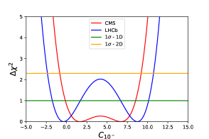
Figure 5: $\Delta\chi^{2}$ as function of $C_{10^{-}}$. The plot shows the impact of LHCb LHCb:2021awg (blue) and CMS CMS:2022mgd (red) measurements on $C_{10^{-}}$ for the 1D (green) and 2D (orange) fits at $1\sigma$.

Appendix A Covariance matrices

Here, we describe the construction of the experimental and theoretical covariance matrices utilized in our analysis. We do not consider correlations between the experimental data and the theory inputs or vice-versa. Hence, the experimental and theoretical covariance matrices are added in Eq. 41. In addition, we do not consider correlations between different observables except for the bins of differential branching ratios of $B^{+}\to\pi^{+}\mu^{+}\mu^{-}$ decays. These assumptions result in the following block-diagonal covariance matrix

$$V^{(X)}=\begin{pmatrix}[V_{B\pi}^{(X)}]_{3\times 3}&0_{3\times 1}&0_{3\times 1}&0_{3\times 1}\\ 0_{1\times 3}&V_{B_{s}\bar{K}^{*}}^{(X)}&0&0\\ 0_{1\times 3}&0&V_{bd\mu}^{(X)}&0\\ 0_{1\times 3}&0&0&V_{bd\gamma}^{(X)}\end{pmatrix},\,$$ (53)

where $V_{B\pi}^{(X)}$, $V_{B_{s}\bar{K}^{*}}^{(X)}$, $V_{bd\mu}^{(X)}$, and $V_{bd\gamma}^{(X)}$ with $X=\text{exp}\,(\text{th})$, are the experimental (theoretical) covariance matrices of the three binned branching fractions $\mathcal{B}^{(B\pi)}_{1,2,9}$, and the branching ratios $\mathcal{B}(B_{s}^{0}\,\to\,\bar{K}^{*0}\,\mu^{+}\mu^{-})$, $\mathcal{B}(B^{0}\,\to\,\mu^{+}\mu^{-})$, and $\mathcal{B}(\bar{B}\,\to\,X_{d}\,\gamma)$, respectively.

A.1 $V^{(\text{exp})}$

The LHCb collaboration LHCb:2015hsa does not provide the statistical and systematic correlation matrices for the block $[V_{B\pi}^{(\text{exp})}]_{3\times 3}$. Therefore, we conservatively assume independent statistical uncertainties and maximally correlated systematic errors,

$$[V_{B\pi}^{(\text{exp})}]_{ij}\,=\,\sigma_{i}^{2}\,\delta_{ij}\,+\,\epsilon_{i}\,\epsilon_{j}~{},$$ (54)

where the statistical $\sigma_{i}$ and systematic $\epsilon_{i}$ uncertainties are provided in Tab. 1. For the other entries $V^{(\text{exp})}_{\alpha}$ with $\alpha=B_{s}\bar{K}^{*},\,bd\mu,\,bd\gamma$, we use $V^{(\text{exp})}_{k}=\sigma^{2}_{\alpha}$ where the experimental errors are taken from Eqs. 18, 23, and 34, respectively.

A.2 $V^{(\text{th})}$

We start with the block $[V_{B\pi}^{(\text{th})}]_{3\times 3}$, where three sources of uncertainty (FFs, CKM matrix elements, and the variation of the short-distance scale $\mu_{b}$) are included as

$$V_{B\pi}^{(\text{th})}\,=\,V_{B\pi}^{(\text{FFs})}\,+\,V_{B\pi}^{(\text{CKM})}\,+\,V_{B\pi}^{(\mu_{b})}\,.$$ (55)

The matrix $V_{B\pi}^{(\text{FFs})}$ can be written as

$$\left[V_{B\pi}^{(\text{FFs})}\right]_{ij}\,=\,\left[\rho^{(\text{FFs})}_{B\pi}\right]_{ij}\,\sigma_{B\pi,\,i}^{(\text{FFs})}\,\sigma_{B\pi,\,j}^{(\text{FFs})}~{},$$ (56)

where $\sigma_{B\pi,\,i}^{(\text{FFs})}$ is the FF uncertainty of $\mathcal{B}_{i}^{(B\pi)}$. In Eq. 56, $[\rho^{(\text{FFs})}_{B\pi}]_{ij}$ denotes the correlation matrix for the FFs between $\mathcal{B}_{i}^{(B\pi)}$ and $\mathcal{B}_{j}^{(B\pi)}$. It can be expressed via the quantity $\Delta\mathcal{B}^{(B\pi)}_{ij}=\mathcal{B}_{i}^{(B\pi)}+\mathcal{B}_{j}^{(B\pi)}$ with the uncertainty $\sigma_{\Delta B\pi,\,ij}^{(\text{FFs})}$, and we write

$$[\rho^{(\text{FFs})}_{B\pi}]_{ij}\,=\,\frac{\left(\sigma_{\Delta B\pi,\,ij}^{(\text{FFs})}\right)^{2}\,-\,\left(\sigma_{B\pi,\,i}^{(\text{FFs})}\right)^{2}\,-\,\left(\sigma_{B\pi,\,j}^{(\text{FFs})}\right)^{2}}{2\,\left(\sigma_{B\pi,\,i}^{(\text{FFs})}\right)\,\left(\sigma_{B\pi,\,j}^{(\text{FFs})}\right)}~{},$$ (57)

with

$$(\sigma_{\Psi}^{(\text{FFs})})^{2}=\sum_{\mathcal{F},\mathcal{F}^{\prime}}\sum_{k,k^{\prime}}\frac{\partial\Psi}{\partial\alpha_{k}^{(\mathcal{F})}}\text{cov}\left(\alpha_{k}^{(\mathcal{F})},\alpha_{k^{\prime}}^{(\mathcal{F}^{\prime})}\right)\frac{\partial\Psi}{\partial\alpha_{k^{\prime}}^{(\mathcal{F}^{\prime})}}~{},$$

where $\Psi$ is a generic function that depends on the parameters $\alpha_{k}^{(\mathcal{F})}$ from the FF $\mathcal{F}$, see Ref. Leljak:2021vte .

Since the main dependence on the CKM matrix elements factorizes, that is $\mathcal{B}_{i}^{(B\pi)}\,=\,\left|V_{tb}\,V_{td}^{*}\right|^{2}\times(...)$, we estimate this uncertainty as

$$\sigma_{B\pi,\,i}^{(\text{CKM})}\,=\,\mathcal{B}_{i}^{(B\pi)}\,\frac{\delta(\left|V_{tb}\,V_{td}^{*}\right|^{2})}{\left|V_{tb}\,V_{td}^{*}\right|^{2}}~{},$$ (58)

where $\delta(\left|V_{tb}\,V_{td}^{*}\right|^{2})$ refers to the uncertainty of $\left|V_{tb}\,V_{td}^{*}\right|^{2}\,=\,(7.3\pm 0.4)\cdot 10^{-5}$ ParticleDataGroup:2022pth . The covariance matrix $V_{B\pi}^{(\text{CKM})}$ is given by

$$[V_{B\pi}^{(\text{CKM})}]_{ij}\,=\,\sigma_{B\pi,\,i}^{(\text{CKM})}\,\sigma_{B\pi,\,j}^{(\text{CKM})}\,\delta_{ij}~{}.$$ (59)

For $V_{B\pi}^{(\mu_{b})}$, we perform a variation of the short-distance scale $\mu_{b}$ between $3$ to $5\,\text{GeV}$ using Table I from Ref. Ali:2013zfa , and estimate the uncertainty of $\mathcal{B}_{i}^{(B\pi)}$ as

$$\sigma_{B\pi,\,i}^{(\mu_{b})}\,=\,\frac{\left|\mathcal{B}_{i}^{(B\pi)}(5\,\text{GeV})-\mathcal{B}_{i}^{(B\pi)}(3\,\text{GeV})\right|}{2}~{}.$$ (60)

We obtain

$$[V_{B\pi}^{(\mu_{b})}]_{ij}\,=\,\sigma_{B\pi,\,i}^{(\mu_{b})}\,\sigma_{B\pi,\,j}^{(\mu_{b})}\,\delta_{ij}~{}.$$ (61)

Adding Eqs. 56, 59, and 61, we obtain $[V_{B\pi}^{(\text{th})}]_{ij}$. For the correlation matrices $V_{B_{s}\bar{K}^{*}}^{(\text{th})}$, $V_{bd\mu}^{(\text{th})}$, and $V_{bd\gamma}^{(\text{th})}$, we follow a similar procedure as the one for $V_{B\pi}^{(\text{th})}$.

Appendix B Cuts in $B_{s}^{0}\to\bar{K}^{*0}\,\mu^{+}\mu^{-}$

Here we estimate the uncertainty due to contributions from $J/\psi$ and $\psi^{\prime}$ resonances in the $B_{s}^{0}\to\bar{K}^{*0}\,\mu^{+}\mu^{-}$ branching ratio, which corresponds to the last uncertainty in Eq. 17. This is necessary to interpret the data LHCb:2018rym , which is provided only for a single large bin encompassing the resonance regions: while kinematic cuts have been applied to remove the bulk of the $J/\psi$ and $\psi^{\prime}$, $q^{2}\in[8,\,11]\,\text{GeV}^{2}$ ($J/\psi$) and $q^{2}\in[12.5,\,15]\,\text{GeV}^{2}$ ($\psi^{\prime}$), their tails enter the signal regions and affect the interpolation between them. We stress that this procedure introduces some degree of model dependence and additional uncertainty and can be avoided once data in theory-friendly bins are available. To make progress we model these effects using a constant-width Breit-Wigner approximation,

$$C_{9}^{\text{res}}(q^{2})=\sum_{R}\frac{a_{R}\,\text{e}^{\text{i}\,\delta_{R}}}{q^{2}-m_{R}^{2}+\text{i}\,m_{R}\,\Gamma_{R}}~{},$$ (62)

with ‘fudge factor’ $a_{R}>0$ and $R=J/\psi,\,\psi^{\prime}$, and $m_{R},\Gamma_{R}$ the resonance mass and width. This simple ansatz serves to estimate the uncertainty of the interpolation but we note that a more sophisticated prescription Kruger:1996cv could be used for the resonance shapes. Close to $q^{2}\approx m_{R}^{2}$, the differential branching ratio is dominated by the resonance $R$, that is

$$\frac{\text{d}\,\mathcal{B}(B_{s}^{0}\to\bar{K}^{*0}\,\mu^{+}\mu^{-})}{\text{d}\,q^{2}}\,\propto\frac{f(q^{2})\,a_{R}^{2}}{(q^{2}-m_{R}^{2})^{2}\,+\,m_{R}^{2}\,\Gamma_{R}^{2}}~{}.$$ (63)

Here, $f(q^{2})$ is a function obtained from Eqs. 14, II.2.2, and II.2.2. In the limit $\Gamma_{R}/m_{R}\to 0$, Eq. 63 becomes a $\delta$-distribution, and integration over $q^{2}$ yields

$$\mathcal{B}(B_{s}^{0}\to\bar{K}^{*0}\,\mu^{+}\mu^{-})\,\propto\,\frac{\pi\,a_{R}^{2}\,f(m_{R}^{2})}{m_{R}\,\Gamma_{R}}~{}.$$ (64)

In this limit, we can only produce the resonance $R$ on-shell, which later on decays to muons

$$\mathcal{B}(B_{s}^{0}\to\bar{K}^{*0}\,\mu^{+}\mu^{-})=\mathcal{B}(B_{s}^{0}\to\bar{K}^{*0}\,R)\,\mathcal{B}(R\to\mu^{+}\mu^{-})~{}.$$ (65)

Using Eqs. 64 and 65, together with the experimental information on $m_{R}$, $\Gamma_{R}$, $\mathcal{B}(B_{s}^{0}\to\bar{K}^{*0}\,R)$, and $\mathcal{B}(R\to\mu^{+}\mu^{-})$ ParticleDataGroup:2022pth , one extracts $a_{R}$ as

$$a_{R}\,=\,\sqrt{\frac{m_{R}\,\Gamma_{R}\,\mathcal{B}(B_{s}^{0}\to\bar{K}^{*0}\,R)\,\mathcal{B}(R\to\mu^{+}\mu^{-})}{\pi\,f(m_{R}^{2})}}~{},$$ (66)

resulting in the fudge factors

$$\begin{split}a_{J/\psi}\,&=\,1.89\pm 0.09~{},\\ a_{\psi^{\prime}}\,&=\,1.20\pm 0.10~{},\end{split}$$ (67)

close to their naive factorization limit $a_{R}\simeq 1$. The only remaining unknowns in Eq. 62 are the phases $\delta_{R}\in[0,\,2\pi]$, and represent the main source of uncertainty.

Figure 6 displays the differential branching ratio $\text{d}\mathcal{B}(B_{s}^{0}\to\bar{K}^{*0}\,\mu^{+}\mu^{-})/\text{d}q^{2}$. The red dashed line depicts the central value of the non-resonant contribution in the SM. The orange region represents the SM prediction with both the non-resonant and the resonant contributions, obtained by scanning over both phase shifts $\delta_{J/\psi,\psi^{\prime}}\in[0,\,2\pi]$. The LHCb LHCb:2018rym veto regions around the $J/\psi$ and $\psi^{\prime}$ resonances are shown as gray-shaded bands. In addition, Fig. 6 shows the central values for those phase shifts that give the maximum/minimum differential branching ratio using the LHCb $q^{2}$-cuts:

• $q^{2}=8\,\text{GeV}^{2}$: maximum ($\delta_{J/\psi}=\pi,\,\delta_{\psi^{\prime}}=\pi$, black solid line) and minimum ($\delta_{J/\psi}=0,\,\delta_{\psi^{\prime}}=0$, black dotted line),

• $q^{2}=11,\,12.5\,\text{GeV}^{2}$: maximum ($\delta_{J/\psi}=0,\,\delta_{\psi^{\prime}}=\pi$, black dashed line) and minimum ($\delta_{J/\psi}=\pi,\,\delta_{\psi^{\prime}}=0$, black dot-dashed line),

• $q^{2}=15\,\text{GeV}^{2}$: maximum ($\delta_{J/\psi}=0,\,\delta_{\psi^{\prime}}=0$, black dotted line) and minimum ($\delta_{J/\psi}=\pi,\,\delta_{\psi^{\prime}}=\pi$, black solid line).

To make use of the data, we exclude the veto regions and interpolate between them and give a conservative estimation of this uncertainty. In Fig. 6, we learn that the effect from resonances tends to cancel between the signal bins [0.1,8], [11,12.5], [15,19] $\text{GeV}^{2}$ for fixed values of $\delta_{R}$. Therefore the resonance contribution on the full bin [0.1,19] $\text{GeV}^{2}$ is dominated by the regions vetoed by the experiment. We numerically cross-checked this assumption, which yields up to $\mathcal{O}\left({10^{-10}}\right)$ corrections, compared to $\mathcal{B}_{\text{total}}\sim\mathcal{O}\left({10^{-8}}\right)$, which is two orders of magnitude larger.

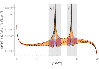
Figure 6: Differential branching ratio of $B^{0}_{s}\to\bar{K}^{*0}\mu^{+}\mu^{-}$ as a function of $q^{2}$. The vertical gray bands around the $J/\Psi$ and the $\psi^{\prime}$ correspond to the regions vetoed by LHCb from the branching ratio measurement LHCb:2018rym . The red dashed line depicts the central value of the non-resonant SM contribution. The orange region illustrates the SM behavior with both the non-resonant and the resonant contributions, obtained by scanning independently over both relative phases $\delta_{J/\psi,\psi^{\prime}}\in[0,\,2\pi]$. Details on the blue and red areas in the veto regions are given in the text.

We hence obtain the residual (interpolation) uncertainty of the resonances $\varepsilon_{\text{model}}$ from the resonance (veto) regions, as

$$\mathcal{B}_{[8,\,11]}^{\text{R}+\text{NR}}+\mathcal{B}_{[12.5,\,15]}^{\text{R}+\text{NR}}\longrightarrow\mathcal{B}_{[8,\,11]}^{\text{NR}}+\mathcal{B}_{[12.5,\,15]}^{\text{NR}}\,+\,\varepsilon_{\text{model}}~{}.$$

It is computed in the following way: For each resonance region ([8,11]$\,\text{GeV}^{2}$ and [12.5,15]$\,\text{GeV}^{2}$) we consider three points to the left and three points to the right of the intervals corresponding to the minimal/maximal value of $\delta_{R}$, and then perform an interpolation between them (blue and red solid lines). Allowing for different strong phases on both sides of the veto intervals (blue region in Fig. 6) gives a more conservative uncertainty estimation than assuming the same strong phases (red region in Fig. 6), that is, the red area is inside the blue one. In the fits we employ the more conservative approach and assume that the strong phases are not correlated and take maximum/minimum values on both sides, corresponding to the blue area. The resulting symmetrized uncertainty of $\varepsilon_{\text{model}}$ is obtained as

$$\varepsilon_{\text{model}}\,=\,\sqrt{(\delta\varepsilon_{J/\psi})^{2}+(\delta\varepsilon_{\psi^{\prime}})^{2}}\,=\,3.6\cdot 10^{-9}~{},$$ (68)

corresponding to the last uncertainty in Eq. 17, with

$$\delta\varepsilon_{J/\psi}\, =\,\frac{1}{2}\int_{8\text{GeV}^{2}}^{11\text{GeV}^{2}}\text{d}q^{2}\,\left(\frac{\text{d}\,\mathcal{B}_{\text{max}}^{[8,11]}}{\text{d}\,q^{2}}-\frac{\text{d}\,\mathcal{B}_{\text{min}}^{[8,11]}}{\text{d}\,q^{2}}\right),$$

$$\delta\varepsilon_{\psi^{\prime}}\, =\,\frac{1}{2}\int_{12.5\text{GeV}^{2}}^{15\text{GeV}^{2}}\text{d}q^{2}\,\left(\frac{\text{d}\,\mathcal{B}_{\text{max}}^{[12.5,15]}}{\text{d}\,q^{2}}-\frac{\text{d}\,\mathcal{B}_{\text{min}}^{[12.5,15]}}{\text{d}\,q^{2}}\right)~{}.$$

For comparison, the model uncertainty on the interpolation for the red region is smaller, $\varepsilon_{\text{model}}=2.2\cdot 10^{-9}$. We also note that the fraction of the full (after cuts and interpolation) to the signal branching ratio is $1.33\pm 0.24$, consistent but with larger uncertainty that the one employed by LHCb from the $B^{0}\to K^{0*}\mu\mu$ analysis, $1.532\pm 0.001\,(\text{stat})\pm 0.010\,(\text{syst})$ LHCb:2016ykl .

Appendix C Global $b\to s$ fits

In this appendix, we provide the results of the global fit to $b\to s\mu^{+}\mu^{-},\gamma$ data including the update on $\mathcal{B}(B_{s}^{0}\to\mu^{+}\mu^{-})$ from the CMS-collaboration CMS:2022mgd . We follow the same approach as Ref. Bause:2021cna , where the python package flavio Straub:2018kue was employed, and refer there for details. We do not include the $R_{K}$ and $R_{K^{*}}$ measurements from LHCb LHCb:2022zom ; LHCb:2022qnv since these observables also include electron modes, and would require lepton-specific fits. We recall that dielectron modes are presently much less probed experimentally than dimuon ones and have therefore also not been included in the $b\to d$ fits presented in this work.

scenario	fit parameter	best fit ($1\sigma$)	$\chi^{2}/\text{dof}$	Pull${}_{H_{i}}$
$H_{3}$	$C_{9}$	$-0.85\pm 0.21$	1.03	3.57
$H_{10}$	$C_{9}=-C_{10}$	$-0.50\pm 0.13$	1.01	4.07
$H_{17}$	$(C_{7},C_{8})$	$(0.01\pm 0.03,-0.25\pm 0.45)$	1.11	0.30
$H_{20}$	$(C_{7},C_{7}^{\prime})$	$(-0.007\pm 0.014,0.02\pm 0.02)$	1.11	0.62
$H_{23}$	$(C_{9},C_{10})$	$(-1.03\pm 0.21,0.41\pm 0.13)$	0.97	4.44
$H_{25}$	$(C_{9},C_{9}^{\prime})$	$(-0.86\pm 0.20,0.54\pm 0.27)$	1.01	3.69
$H_{26}$	$(C_{9},C_{10}^{\prime})$	$(-1.09\pm 0.19,-0.37\pm 0.10)$	0.95	4.85
$H_{28}$	$(C_{9}^{\prime},C_{10})$	$(0.38\pm 0.23,0.30\pm 0.13)$	1.06	2.60
$H_{29}$	$(C_{10},C_{10}^{\prime})$	$(0.22\pm 0.18,-0.10\pm 0.15)$	1.07	2.15
$H_{32}$	$(C_{9}^{\prime},C_{10}^{\prime})$	$(0.24\pm 0.25,-0.18\pm 0.11)$	1.08	2.04

Table 9: Fit results of Wilson coefficients $C_{i}^{(b\to s)}$ to $b\to s\mu^{+}\mu^{-},\gamma$ data for some exemplary 1D and 2D scenarios at the scale $\mu_{b}$. Best-fit values with its $1\sigma$ uncertainties are displayed in the third column. We also provide the $\chi^{2}/\text{dof}$ value and respective pull from the SM hypothesis.

References

- (1) S. Bifani, S. Descotes-Genon, A. Romero Vidal, and M.-H. Schune, Review of Lepton Universality tests in decays, J. Phys. G 46 (2019), no. 2 023001, [arXiv:1809.06229].
- (2) J. Albrecht, D. van Dyk, and C. Langenbruch, Flavour anomalies in heavy quark decays, Prog. Part. Nucl. Phys. 120 (2021) 103885, [arXiv:2107.04822].
- (3) D. London and J. Matias, Flavour Anomalies: 2021 Theoretical Status Report, arXiv:2110.13270.
- (4) M. Algueró, B. Capdevila, S. Descotes-Genon, J. Matias, and M. Novoa-Brunet, global fits after and , Eur. Phys. J. C 82 (2022), no. 4 326, [arXiv:2104.08921].
- (5) J. Kriewald, C. Hati, J. Orloff, and A. M. Teixeira, Leptoquarks facing flavour tests and after Moriond 2021, in 55th Rencontres de Moriond on Electroweak Interactions and Unified Theories, 3, 2021. arXiv:2104.00015.
- (6) L.-S. Geng, B. Grinstein, S. Jäger, S.-Y. Li, J. Martin Camalich, and R.-X. Shi, Implications of new evidence for lepton-universality violation in b→s+- decays, Phys. Rev. D 104 (2021), no. 3 035029, [arXiv:2103.12738].
- (7) R. Bause, H. Gisbert, M. Golz, and G. Hiller, Interplay of dineutrino modes with semileptonic rare B-decays, JHEP 12 (2021) 061, [arXiv:2109.01675].
- (8) LHCb Collaboration, R. Aaij et al., Test of lepton universality in beauty-quark decays, Nature Phys. 18 (2022), no. 3 277–282, [arXiv:2103.11769].
- (9) G. Hiller and F. Kruger, More model-independent analysis of processes, Phys. Rev. D 69 (2004) 074020, [hep-ph/0310219].
- (10) LHCb Collaboration, Measurement of lepton universality parameters in and decays, arXiv:2212.09153.
- (11) LHCb Collaboration, Test of lepton universality in decays, arXiv:2212.09152.
- (12) LHCb Collaboration, R. Aaij et al., First measurement of the differential branching fraction and asymmetry of the decay, JHEP 10 (2015) 034, [arXiv:1509.00414].
- (13) LHCb Collaboration, R. Aaij et al., Measurement of the decay properties and search for the and decays, Phys. Rev. D 105 (2022), no. 1 012010, [arXiv:2108.09283].
- (14) LHCb Collaboration, R. Aaij et al., Evidence for the decay , JHEP 07 (2018) 020, [arXiv:1804.07167].
- (15) M. Misiak et al., Updated NNLO QCD predictions for the weak radiative B-meson decays, Phys. Rev. Lett. 114 (2015), no. 22 221801, [arXiv:1503.01789].
- (16) BaBar Collaboration, P. del Amo Sanchez et al., Study of Decays and Determination of , Phys. Rev. D 82 (2010) 051101, [arXiv:1005.4087].
- (17) D. Du, A. X. El-Khadra, S. Gottlieb, A. S. Kronfeld, J. Laiho, E. Lunghi, R. S. Van de Water, and R. Zhou, Phenomenology of semileptonic B-meson decays with form factors from lattice QCD, Phys. Rev. D 93 (2016), no. 3 034005, [arXiv:1510.02349].
- (18) A. Ali, A. Y. Parkhomenko, and A. V. Rusov, Precise Calculation of the Dilepton Invariant-Mass Spectrum and the Decay Rate in in the SM, Phys. Rev. D 89 (2014), no. 9 094021, [arXiv:1312.2523].
- (19) A. V. Rusov, Probing New Physics in transitions, JHEP 07 (2020) 158, [arXiv:1911.12819].
- (20) W. Buchmuller and D. Wyler, Effective Lagrangian Analysis of New Interactions and Flavor Conservation, Nucl. Phys. B 268 (1986) 621–653.
- (21) B. Grzadkowski, M. Iskrzynski, M. Misiak, and J. Rosiek, Dimension-Six Terms in the Standard Model Lagrangian, JHEP 10 (2010) 085, [arXiv:1008.4884].
- (22) S. Bißmann, C. Grunwald, G. Hiller, and K. Kröninger, Top and Beauty synergies in SMEFT-fits at present and future colliders, JHEP 06 (2021) 010, [arXiv:2012.10456].
- (23) R. Bause, H. Gisbert, M. Golz, and G. Hiller, Lepton universality and lepton flavor conservation tests with dineutrino modes, Eur. Phys. J. C 82 (2022), no. 2 164, [arXiv:2007.05001].
- (24) S. Bruggisser, R. Schäfer, D. van Dyk, and S. Westhoff, The Flavor of UV Physics, JHEP 05 (2021) 257, [arXiv:2101.07273].
- (25) C. Bobeth, M. Misiak, and J. Urban, Photonic penguins at two loops and dependence of , Nucl. Phys. B 574 (2000) 291–330, [hep-ph/9910220].
- (26) H. H. Asatrian, H. M. Asatrian, C. Greub, and M. Walker, Two loop virtual corrections to in the standard model, Phys. Lett. B 507 (2001) 162–172, [hep-ph/0103087].
- (27) H. H. Asatryan, H. M. Asatrian, C. Greub, and M. Walker, Calculation of two loop virtual corrections to in the standard model, Phys. Rev. D 65 (2002) 074004, [hep-ph/0109140].
- (28) A. Ali, E. Lunghi, C. Greub, and G. Hiller, Improved model independent analysis of semileptonic and radiative rare decays, Phys. Rev. D 66 (2002) 034002, [hep-ph/0112300].
- (29) H. M. Asatrian, K. Bieri, C. Greub, and M. Walker, Virtual corrections and bremsstrahlung corrections to b — d l+ l- in the standard model, Phys. Rev. D 69 (2004) 074007, [hep-ph/0312063].
- (30) S. de Boer, Two loop virtual corrections to and for arbitrary momentum transfer, Eur. Phys. J. C 77 (2017), no. 11 801, [arXiv:1707.00988].
- (31) A. Ali, P. Ball, L. T. Handoko, and G. Hiller, A Comparative study of the decays (, in standard model and supersymmetric theories, Phys. Rev. D 61 (2000) 074024, [hep-ph/9910221].
- (32) T. Hurth, E. Lunghi, and W. Porod, Untagged CP asymmetry as a probe for new physics, Nucl. Phys. B 704 (2005) 56–74, [hep-ph/0312260].
- (33) C. Bobeth, G. Hiller, and G. Piranishvili, Angular distributions of decays, JHEP 12 (2007) 040, [arXiv:0709.4174].
- (34) M. Beneke, T. Feldmann, and D. Seidel, Exclusive radiative and electroweak and penguin decays at NLO, Eur. Phys. J. C 41 (2005) 173–188, [hep-ph/0412400].
- (35) B. Grinstein and D. Pirjol, Exclusive rare decays at low recoil: Controlling the long-distance effects, Phys. Rev. D 70 (2004) 114005, [hep-ph/0404250].
- (36) C. Bobeth, G. Hiller, D. van Dyk, and C. Wacker, The Decay at Low Hadronic Recoil and Model-Independent Constraints, JHEP 01 (2012) 107, [arXiv:1111.2558].
- (37) W.-S. Hou, M. Kohda, and F. Xu, Rates and asymmetries of B→+- decays, Phys. Rev. D 90 (2014), no. 1 013002, [arXiv:1403.7410].
- (38) A. Ali, A. Parkhomenko, and I. Parnova, Impact of weak annihilation contribution on rare semileptonic decay, J. Phys. Conf. Ser. 1690 (2020), no. 1 012162.
- (39) D. Leljak, B. Melić, and D. van Dyk, The → form factors from QCD and their impact on |Vub|, JHEP 07 (2021) 036, [arXiv:2102.07233].
- (40) C. Hambrock, A. Khodjamirian, and A. Rusov, Hadronic effects and observables in decay at large recoil, Phys. Rev. D 92 (2015), no. 7 074020, [arXiv:1506.07760].
- (41) Fermilab Lattice, MILC Collaboration, J. A. Bailey et al., form factors for new-physics searches from lattice QCD, Phys. Rev. Lett. 115 (2015), no. 15 152002, [arXiv:1507.01618].
- (42) N. Gubernari, A. Kokulu, and D. van Dyk, and Form Factors from -Meson Light-Cone Sum Rules beyond Leading Twist, JHEP 01 (2019) 150, [arXiv:1811.00983].
- (43) M. Beneke, C. Bobeth, and R. Szafron, Power-enhanced leading-logarithmic QED corrections to , JHEP 10 (2019) 232, [arXiv:1908.07011]. [Erratum: JHEP 11, 099 (2022)].
- (44) Particle Data Group Collaboration, R. L. Workman et al., Review of Particle Physics, PTEP 2022 (2022) 083C01.
- (45) K. De Bruyn, R. Fleischer, R. Knegjens, P. Koppenburg, M. Merk, A. Pellegrino, and N. Tuning, Probing New Physics via the Effective Lifetime, Phys. Rev. Lett. 109 (2012) 041801, [arXiv:1204.1737].
- (46) A. Di Canto and S. Meinel, Weak Decays of and Quarks, arXiv:2208.05403.
- (47) A. Crivellin and L. Mercolli, and constraints on new physics, Phys. Rev. D 84 (2011) 114005, [arXiv:1106.5499].
- (48) P. Gambino and M. Misiak, Quark mass effects in anti-B — X(s gamma), Nucl. Phys. B 611 (2001) 338–366, [hep-ph/0104034].
- (49) H. Dembinski and P. O. et al., scikit-hep/iminuit, .
- (50) S. Descotes-Genon, L. Hofer, J. Matias, and J. Virto, Global analysis of anomalies, JHEP 06 (2016) 092, [arXiv:1510.04239].
- (51) C. Bobeth, G. Hiller, and D. van Dyk, The Benefits of Decays at Low Recoil, JHEP 07 (2010) 098, [arXiv:1006.5013].
- (52) A. Ali, G. F. Giudice, and T. Mannel, Towards a model independent analysis of rare decays, Z. Phys. C 67 (1995) 417–432, [hep-ph/9408213].
- (53) Belle Collaboration, A. Ishikawa et al., Measurement of Forward-Backward Asymmetry and Wilson Coefficients in B — K* l+ l-, Phys. Rev. Lett. 96 (2006) 251801, [hep-ex/0603018].
- (54) J. Fuentes-Martin, A. Greljo, J. Martin Camalich, and J. D. Ruiz-Alvarez, Charm physics confronts high-pT lepton tails, JHEP 11 (2020) 080, [arXiv:2003.12421].
- (55) A. Angelescu, D. A. Faroughy, and O. Sumensari, Lepton Flavor Violation and Dilepton Tails at the LHC, Eur. Phys. J. C 80 (2020), no. 7 641, [arXiv:2002.05684].
- (56) Belle Collaboration, J. Grygier et al., Search for decays with semileptonic tagging at Belle, Phys. Rev. D 96 (2017), no. 9 091101, [arXiv:1702.03224]. [Addendum: Phys.Rev.D 97, 099902 (2018)].
- (57) A. Cerri et al., Report from Working Group 4: Opportunities in Flavour Physics at the HL-LHC and HE-LHC, CERN Yellow Rep. Monogr. 7 (2019) 867–1158, [arXiv:1812.07638].
- (58) Belle-II Collaboration, W. Altmannshofer et al., The Belle II Physics Book, PTEP 2019 (2019), no. 12 123C01, [arXiv:1808.10567]. [Erratum: PTEP 2020, 029201 (2020)].
- (59) FCC Collaboration, A. Abada et al., FCC Physics Opportunities: Future Circular Collider Conceptual Design Report Volume 1, Eur. Phys. J. C 79 (2019), no. 6 474.
- (60) A. Biswas, S. Nandi, S. K. Patra, and I. Ray, Study of the transitions in the Standard Model and test of New Physics sensitivities, arXiv:2208.14463.
- (61) CMS Collaboration, Measurement of the B decay properties and search for the B0 decay in proton-proton collisions at = 13 TeV, arXiv:2212.10311.
- (62) F. Kruger and L. M. Sehgal, Lepton polarization in the decays b — X(s) mu+ mu- and B — X(s) tau+ tau-, Phys. Lett. B 380 (1996) 199–204, [hep-ph/9603237].
- (63) LHCb Collaboration, R. Aaij et al., Measurements of the S-wave fraction in decays and the differential branching fraction, JHEP 11 (2016) 047, [arXiv:1606.04731]. [Erratum: JHEP 04, 142 (2017)].
- (64) D. M. Straub, flavio: a Python package for flavour and precision phenomenology in the Standard Model and beyond, arXiv:1810.08132.