Self-gravitating disks around rapidly spinning, tilted black holes: General relativistic simulations

Abstract

We perform general relativistic simulations of self-gravitating black hole-disks in which the spin of the black hole is significantly tilted ($45^{\circ}$ and $90^{\circ}$) with respect to the angular momentum of the disk and the disk-to-black hole mass ratio is $16\%-28\%$. The black holes are rapidly spinning with dimensionless spins up to $\sim 0.97$. These are the first self-consistent hydrodynamic simulations of such systems, which can be prime sources for multimessenger astronomy. In particular tilted black hole-disk systems lead to: i) black hole precession; ii) disk precession and warping around the black hole; iii) earlier saturation of the Papaloizou-Pringle instability compared to aligned/antialigned systems, although with a shorter mode growth timescale; iv) acquisition of a small black-hole kick velocity; v) significant gravitational wave emission via various modes beyond, but as strong as, the typical $(2,2)$ mode; and vi) the possibility of a broad alignment of the angular momentum of the disk with the black hole spin. This alignment is not related to the Bardeen-Petterson effect and resembles a solid body rotation. Our simulations suggest that any electromagnetic luminosity from our models may power relativistic jets, such as those characterizing short gamma-ray bursts. Depending on the black hole-disk system scale the gravitational waves may be detected by LIGO/Virgo, LISA and/or other laser interferometers.

I Introduction

Black holes (BHs) immersed in gaseous environments are ubiquitous in the Universe. Black hole-disks (BHDs) appear on a great variety of scales, reflecting their diverse birth channels and sites. From the core collapse of massive stars Woosley (1993); MacFadyen and Woosley (1999) and the cores of active galactic nuclei Lynden-Bell (1969); Shakura and Sunyaev (1973); Paczynski (1978), to asymmetric supernova explosions in binary systems Fragos et al. (2010), and the merger of compact binaries where at least one of the companions is not a BH, BHDs may be formed and serve as prime candidates for multimessenger astronomy.

The magnitude of the spin of the BH, as well as its orientation relative to the fluid flow, can have large effects, as in the existence and geometry of a relativistic plasma jet (see e.g. Liska et al. (2018)). This jet, which can be powered either by magnetic fields threading the event horizon and extracting rotational energy from the BH Blandford and Znajek (1977a), or from the accretion flow Blandford and Payne (1982), can precess when misalignment between the BH and disk angular momentum arises Aalto et al. (2016); Abraham (2018); Liska et al. (2018). Such misalignment is expected to be a common phenomenon Fragile et al. (2001) both in active galactic nuclei as well as in BH X-ray binaries Hjellming and Rupen (1995); Greene et al. (2001); Maccarone (2002); Caproni et al. (2006); Fragos et al. (2010); Aalto et al. (2016); Abraham (2018); Russell et al. (2019). Even in the recent observation of M87 by the Event Horizon Telescope Akiyama et al. (2019) misalignment could not be excluded Chatterjee et al. (2020); Park et al. (2019).

Tilted BHDs are also the outcome from stellar-mass compact object collisions when their individual spins are not aligned with the orbital angular momentum Foucart et al. (2011, 2013); Kawaguchi et al. (2015); Dietrich et al. (2018); Chaurasia et al. (2020). Population synthesis studies suggest that in approximately half of the BH-neutron star binaries the angle between the orbital angular momentum and the BH spin is larger than $45^{\circ}$ Belczynski et al. (2008). Such systems will yield misaligned BHDs which in turn will affect the existence and the properties of an electromagnetic counterpart, such as a short gamma-ray burst or a kilonova.

Central to the analysis of a tilted BHD is the so-called Lense-Thirring (LT) precession Lense and Thirring (1918), a gravitomagnetic (GM) effect, according to which frame-dragging produced by the rotating and tilted BH causes precession of a test ring with angular velocity $\Omega_{\rm GM-ring}\approx 2GJ_{\rm bh}/(c^{2}r^{3})$, where $J_{\rm bh}$ is the BH angular momentum, and $r$ the ring radius. In the presence of viscosity (as, for example, created by a magnetic field) the cumulative effect of LT precession and internal disk viscosity torques, is the alignment of the angular momenta of the BH and the disk, a phenomenon known as the Bardeen-Petterson (BP) effect Bardeen and Petterson (1975). Due to the rapid fall-off behavior of the LT angular velocity, this alignment only affects the inner parts of the disk, within the so-called Bardeen-Petterson radius, while the outer parts keep their initial orientation. The LT and BP effects have been invoked to explain the quasiperiodic oscillations van der Klis (2005) observed in the X-ray brightness of a number of neutron star and BH X-ray binaries Stella and Vietri (1998); Marković  and Lamb (1998); Fragile et al. (2001); Ingram et al. (2009). Similarly the GM field will make the BH precess around the disk’s rotation axis. This effect has been invoked to explain the precession of jets in tidal disruption events (where a star is tidally disrupted by a supermassive BH) Stone and Loeb (2012). Even in the absence of a jet, the precession of such disks may have observable consequences.

In general, BHD systems (tilted or not) are subject to various instabilities that can lead to significant accretion and ablate away the disk. One such instability is the so-called dynamical runaway instability Abramowicz et al. (1983) where the overflow of a potential surface (similar to the Roche lobe) by the disk matter will lead to a cascading instability and the final consumption of the disk by the BH Font and Daigne (2002); Daigne and Font (2004); Korobkin et al. (2013). In binary mergers where a BHD is the final remnant, it was found Rezzolla et al. (2010); Hotokezaka et al. (2013) that the axisymmetric runaway instability is of limited importance due to the power-law dependence of the specific angular momentum profile of the disk Daigne and Font (2004). Therefore its influence in the formation of ultrarelativistic jets is probably negligible Paschalidis et al. (2015); Ruiz et al. (2016, 2018a, 2021).

A less dramatic instability was discovered by Papaloizou and Pringle Papaloizou and Pringle (1984) that transports angular momentum outwards and leads to the formation of an one-arm instability, the so-called Papaloizou-Pringle instability (PPI). Using perturbation theory, the authors found a quartic algebraic equation for the angular velocity of the perturbation mode whose solutions contain 2 stable modes (real solutions) and 2 unstable ones (imaginary solutions). These wave perturbations depend on the inner and outer radii of the disk Blaes and Glatzel (1986); Balbus (2003) and highlight the importance of these boundaries in the development of the PPI. The instability manifests itself when the a wave which is traveling backwards relative to the fluid at the inner edge exchanges energy and angular momentum with the wave which is traveling forwards relative to the fluid at the outer edge. Angular momentum is transferred outwards, making the wave at the outer edge that has positive angular momentum grow in amplitude while the one in the inner edge that has negative angular momentum also grow in amplitude, since it is losing angular momentum Papaloizou and Pringle (1985); Zurek and Benz (1986); Goldreich et al. (1986); Blaes (1987); Hawley (1987); Goodman et al. (1987); Hawley (1991); Papaloizou and Lin (1995); Goodman and Rafikov (2001); Heinemann and Papaloizou (2012). A similar mechanism in rotating stars leads to the Chandrasekhar–Friedmann–Schutz instability Chandrasekhar (1970); Friedman and Schutz (1978); Friedman (1978) which is induced by gravitational radiation. The PPI, which was originally found in constant specific angular momentum disks, can also be developed in BHDs with a nonconstant specific angular momentum ($\ell$) profile Papaloizou and Pringle (1985). Newtonian analysis finds disks with $\ell\sim r^{q}$ where $q<2-\sqrt{3}=0.266$ to be unstable, where the critical exponent $q$ could be even smaller, i.e. $q\sim 0.25$ Zurek and Benz (1986). In general the growth of the nonaxisymmetric instability is more efficient for a smaller exponent $q$ Zurek and Benz (1986); Balbus (2003). Accretion onto the BH has a stabilizing effect on the PPI since the waves at the inner boundary are disturbed Blaes (1987); Hawley (1991); De Villiers and Hawley (2002). This is especially true for wide disks, while in more slender ones the PPI seems to be less affected Blaes and Hawley (1988).

The first full general relativistic simulations of a tilted thick disk onto a Kerr BH Fragile and Anninos (2005) have demonstrated that LT precession results in a torque that tends to twist and warp the disk, similar to Newtonian studies Nelson and Papaloizou (2000). The authors found that this precession depends primarily on the sound speed in the disk. For disks where in their bulk the LT timescale was less than the azimuthal sound crossing time, the disk undergoes differential precession out to a transition radius. On the other hand when the the LT timescale was greater than the azimuthal sound crossing time, the disk undergoes near rigid-body precession after a short initial period of differential precession. Another interesting finding in Fragile and Anninos (2005) was the tendency for these disks to align toward the equatorial plane of the BH, despite the lack of viscous angular momentum transport. According to the authors this alignment between the angular momentum of the disk and the BH spin was facilitated by the preferential accretion of highly tilted disk material that resulted in the depletion of the misaligned disk angular momentum. Since the authors considered disks with mass much smaller than the BH (test-fluid limit) the spin of the BH was unaffected. Such kind of purely hydrodynamical alignment has also been found in BH-neutron star simulations Kawaguchi et al. (2015), where the alignment timescale was of the same order as the disk precession timescale. The authors speculated that this BP-like behavior is induced by a purely hydrodynamical mechanism, such as angular momentum redistribution due to a nonaxisymmetric shock wave excited in the disk.

The assumption that the mass of the disk is negligible in comparison with the mass of the central BH may not always be valid. Some isolated or binary BHs detectable by LISA may find themselves immersed in extended disks with masses comparable or greater than the BHs themselves. This may be particularly true of stellar-mass BHs in AGNs and quasars or supermassive BHs in extended disks formed in nascent or merging galactic nuclei. The gravitational pull of the disk on the binary can be important in such cases, the accretion rate from the inner disk radius can be high and even super-Eddington, orbital and spin precession as well as spin flipping in the case of misaligned disks is a possibility, while density perturbations in the disk can arise from instabilities. Alternative scenarios for the formation of massive BHDs include the collapse of rapidly rotating, supermassive stars or the merger of binary stellar systems (such as a neutron star-white dwarf) with significant asymmetry in their mass or spin. In binaries the mass of the disk depends on how far from the BH is the secondary compact object being disrupted Foucart (2012). If tidal disruption happens far from the innermost stable circular orbit (ISCO) of the BH, then a disk with a large mass is produced. On the other hand, small mass disks (or even essentially no disk at all) are produced when tidal disruption happens close to the ISCO of the BH (or inside it). This crucial distance that controls the importance of self-gravitation for the disk depends on the mass ratio of the binary, the compactness of the primary and the BH spin. The mass of the disk increases with a larger BH spin (since the ISCO decreases with increasing spin) and decreases with a larger BH mass (the ISCO increases with increasing BH mass) Rezzolla et al. (2010); Lovelace et al. (2013).

Only by including self-gravity in full general relativity and tracking the nonaxisymmetric perturbations that self-gravity may trigger can gravitational waves from the disk be calculated reliably. Such perturbations and gravitational waves can be detected by LISA and other instruments Montero et al. (2010); Kiuchi et al. (2011); Mewes et al. (2016, 2016); Wessel et al. (2021); Shibata et al. (2021a). Also, disk self-gravity must be incorporated to determine the astrophysical consequences of BH precession, which may, for example, trigger X-shape radio galaxies Ekers et al. (1978); Cheung (2007); Bera et al. (2020).

General relativistic studies of self-gravitating BHDs have been performed in a number of works Montero et al. (2010); Kiuchi et al. (2011); Korobkin et al. (2011, 2013); Mewes et al. (2016, 2016); Wessel et al. (2021); Shibata et al. (2021b) and the roles of the runaway instability, as well as the PPI, have been elucidated. Although most of the BHDs will not develop the runaway instability (e.g. Montero et al. (2010); Rezzolla et al. (2010); Kiuchi et al. (2011); Korobkin et al. (2011)), it cannot be excluded when more favorable circumstances are present Korobkin et al. (2013) (e.g. disks that fill their Roche lobes). Regarding the PPI, it was found that, as in Newtonian gravity, self-gravitating BHDs are subject to an $m=1$ nonaxisymmetric mode growth under a wide range of conditions . In Korobkin et al. (2011) it was shown explicitly that the $m=1$ PPI mode is accompanied by an outspiraling motion of the BH, which further amplifies the one-arm instability. More massive tori and a constant specific angular momentum profile favors the appearance of the PPI, in contrast with less massive disks and/or a non-constant $\ell$ profile, for which the disk may even be PP-stable Kiuchi et al. (2011). In addition since the nonaxisymmetric structure survives long after the saturation of the PPI, these systems can be promising sources for coincident detections of electromagnetic and gravitational waves similar to GW170817. The above works focused on tori around nonspinning BHs and were later extended to BHDs around spinning BHs in Mewes et al. (2016); Wessel et al. (2021); Shibata et al. (2021b). In Wessel et al. (2021) it was speculated that the accretion rate in PPI unstable disks may be used to measure the BH spin. It was found that systems of $\sim 10M_{\odot}$ –relevant for for BH–neutron star mergers– will be detectable by the Cosmic Explorer out to $\sim 300$ Mpc, while DECIGO (LISA) will be able to detect systems of $\sim 1000M_{\odot}\ (10^{5}M_{\odot})$. The latter are relevant for disks forming in collapsing, supermassive stars out to cosmological redshift of $z\sim 5\ (z\sim 1)$. In Shibata et al. (2021b) an alternative scenario for event GW190521 was put forward. In particular it was conjectured that GW190521 may not represent the merger of binary BHs, but instead the stellar collapse of a very massive star, leading temporarily to a BH of mass $\sim 50M_{\odot}$ and a massive disk of several tens of solar masses that is dynamically unstable to the PPI.

The first general relativistic simulations where the spin of the BH is tilted with respect to the angular momentum of the disk were performed in Mewes et al. (2016, 2016), albeit starting from artificial initial values. In particular the authors first computed models of self-gravitating, massive tori around nonrotating BHs Stergioulas (2011), and then replaced the resulting spacetime with a tilted Kerr metric in quasi-isotropic coordinates, while retaining the hydrodynamical profile. Notwithstanding these initial conditions the authors performed a thorough investigation of the twist (precession) and the tilt (inclination) of the disk, finding that for BHD mass ratios of $\gtrsim 4\%$ the assumption of using a fixed background spacetime is unjustified. The authors observed significant precession and nutation of the tilted BH as a result of the disk evolution, which cannot be accounted in fixed spacetime simulations. The LT torque that the BH exerts on the disk forces the disk to precess as a solid body which in turn leads to BH precession. The simulations of Mewes et al. (2016, 2016) showed the universal character of the PPI with regards to initial spin magnitudes, tilt angles, and disk angular momentum profiles.

In this work we extend previous studies of self-gravitating BHDs in two ways. For the first time we perform general relativistic simulations of tilted BHDs starting from self-consistent initial values. The tilted BHD models are solutions of the full (i.e. including the conformal metric) general relativistic initial value problem as described in Tsokaros et al. (2019). Second, we extend the parameter space by evolving disks around rapidly spinning BHs (aligned, antialigned and tilted with respect to the disk angular momentum) having dimensionless spins up to $0.97$. We find that although the saturation of the PPI appears significantly earlier for tilted BHDs than those with aligned/antialigned spins, due to the inherent initial nonaxisymmetry, their growth rate is smaller. The maximum density in the disk can increase by orders of magnitude, while the disk precesses and warps around the BH. The BH itself also precesses and its spin can increase or decrease depending the initial configuration. In one case where the initial BH spin was tilted at $45^{\circ}$ with respect to the angular momentum of the disk the BH was spun up to a maximal value, beyond which we couldn’t continue our simulation. In another case where the initial BH spin was tilted by $90^{\circ}$ accretion spun down the BH. By computing the precession timescales we confirmed their agreement with post-Newtonian estimates. The precessing BHDs are responsible for copious gravitational wave emission in multiple modes, which we compute. In general the gravitational wave strain appears to be an order of magnitude larger than previous calculations Kiuchi et al. (2011); Mewes et al. (2016); Wessel et al. (2021); Shibata et al. (2021b) with a diverse spectrum. Although our simulations do not include magnetic fields, estimation of the effective turbulent magnetic viscous timescale shows that it is much longer than the dynamical timescale of the one-arm instability. Therefore we expect these BHDs to be prominent sources of gravitational waves and Poynting electromagnetic radiation (in the presence of magnetic fields) and thus excellent sources for multimessenger astronomy.

In this paper, spacetime indices are Greek, spatial indices Latin, and we employ geometric units in which $G=c=M_{\odot}=1$, unless stated otherwise.

II Initial data

Table 1: The initial BHD models. The angular momentum of the disks is along the z-axis. Columns are the model name, the magnitude of the dimensionless BH spin $\chi=J_{\rm bh}/M_{\rm bh}^{2}$, the angles of the spin angular momentum in spherical coordinates $(\theta_{s},\phi_{s})$, the inner specific angular momentum $\ell_{\rm in}$, the inner edge of the disk $r_{\rm in}$, the maximum density coordinate $r_{c}$, the outer edge of the disk $r_{\rm out}$, the rest mass of the disk $M_{0}$, the Arnowitt-Desser-Misner (ADM) mass $M$, the period of the maximum density point of the disk $P_{c}$, the dynamical time $t_{d}\sim 1/\sqrt{\rho_{\rm max}}$, and the precession angular velocity $P_{\rm GM}$ of the BH as calculated in Sec. II.1. Here $M_{\rm bh}$ is the mass of the BH. Center dots denote “not applicable”.

Model	$\chi$	$(\theta_{s},\phi_{s})$	$\ell_{\rm in}/M_{\rm bh}$	$r_{\rm in}/M_{\rm bh}$	$r_{c}/M_{\rm bh}$	$r_{\rm out}/M_{\rm bh}$	$M_{0}/M_{\rm bh}$	$M/M_{\rm bh}$	$P_{c}/M_{\rm bh}$	$t_{d}/M_{\rm bh}$	$P_{\rm GM}/P_{c}$
A1	$0.966$	$(0^{\circ},0^{\circ})$	$4.63$	$10$	$17.3$	$49.4$	$0.259$	$1.273$	$462$	$297$	$\cdots$
A2	$0.957$	$(45^{\circ},0^{\circ})$	$4.60$	$10$	$17.3$	$49.4$	$0.156$	$1.167$	$435$	$371$	$60$
A3	$0.968$	$(90^{\circ},0^{\circ})$	$4.85$	$10$	$17.9$	$51.1$	$0.280$	$1.298$	$455$	$290$	$35$
A4	$0.963$	$(180^{\circ},0^{\circ})$	$5.13$	$10$	$20.0$	$57.3$	$0.242$	$1.256$	$520$	$364$	$\cdots$

The initial models of the BHDs considered in this work, models A1-A4 in Table 1, have been constructed using the COCAL code and the method described in Tsokaros et al. (2019). In particular we solve the full initial value Einstein equations by assuming that the conformal 3-dim metric is decomposed as $\tilde{\gamma}_{ij}:=f_{ij}+h_{ij}$, where $f_{ij}$ is the flat metric and $h_{ij}$ the nonflat contributions. The metric on the 3-geometry $\gamma_{ij}$ is related to the conformal metric through $\gamma_{ij}=\psi^{4}\tilde{\gamma}_{ij}$. The nonflat contributions $h_{ij}$ are computed alongside the lapse $\alpha$, shift $\beta^{i}$, and the conformal factor $\psi$, assuming ${\rm det}(\tilde{\gamma}_{ij})={\rm det}(f_{ij})$. One of the new characteristics of this method is the decomposition of the conformal tracefree part of the extrinsic curvature as

$$\tilde{A}_{ij}=\tilde{A}^{\rm\scriptscriptstyle KS}_{ij}+\tilde{\sigma}(\tilde{\mathbb{L}}\tilde{W})_{ij},$$ (1)

where $\tilde{A}^{\rm\scriptscriptstyle KS}_{ij}$ is the conformal Kerr-Schild tracefree part, $\tilde{W}_{i}$ an unknown spatial vector, $\tilde{\sigma}$ a scalar, and $\tilde{\mathbb{L}}$ the conformal Killing operator: $(\tilde{\mathbb{L}}\tilde{W})_{ij}=\tilde{D}_{i}\tilde{W}_{j}+\tilde{D}_{j}\tilde{W}_{i}-\frac{2}{3}\tilde{\gamma}_{ij}\tilde{D}_{k}\tilde{W}^{k}$. Here $\tilde{D}_{i}$ is the covariant derivative with respect to the conformal metric $\tilde{\gamma}_{ij}$. It is assumed that $A_{ij}=\psi^{4}\tilde{A}_{ij}$ and $\tilde{\sigma}=1/(2\alpha)$. As explained in Tsokaros et al. (2019), Eq. (1) with the appropriate boundary conditions for $\tilde{W}_{i}$ yields a convergent solution for the potentials $h_{ij}$, which in addition, can be horizon penetrating. The price paid for this additional decomposition of the extrinsic curvature is an extra 3 elliptic equations for the potentials $\tilde{W}_{i}$. For the slicing we assume Kerr-Schild coordinates with $K=K_{\rm\scriptscriptstyle KS}$ under the gauge ${\raise 3.44444pt\hbox{${}^{\ \scalebox{0.7}{$\circ$}}$}}D_{i}h^{ij}={\raise 3.44444pt\hbox{${}^{\ \scalebox{0.7}{$\circ$}}$}}D_{i}h^{ij}_{\rm\scriptscriptstyle KS}$, with $h^{ij}_{\rm\scriptscriptstyle KS}$ being the exact Kerr-Schild potentials, and ${\raise 3.44444pt\hbox{${}^{\ \scalebox{0.7}{$\circ$}}$}}D_{i}$ the covariant derivative with respect to the flat metric $f_{ab}$. We set $\partial_{t}\tilde{\gamma}_{ij}=\partial_{t}\tilde{A}_{ij}=\partial_{t}K=0$.

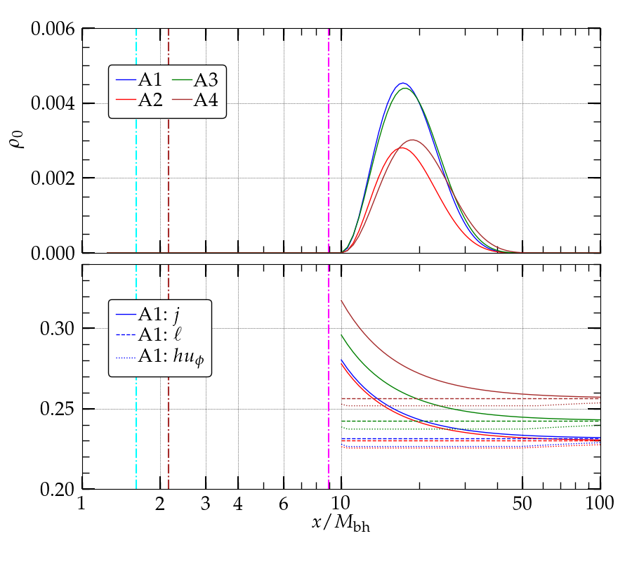
Figure 1: Top panel: Initial rest-mass density distribution for the four models evolved. Bottom panel: The specific angular momentum of the BHD model A1. Solid lines correspond to $j$, dashed lines to $\ell$ and dotted lines to $hu_{\phi}$. The vertical dashed dotted lines correspond to the event horizon (cyan), the marginally stable radius for the prograde orbit (brown), and the marginally stable radius for the retrograde orbit (magenta) around a BH whose dimensionless spin is $\chi=0.95$.

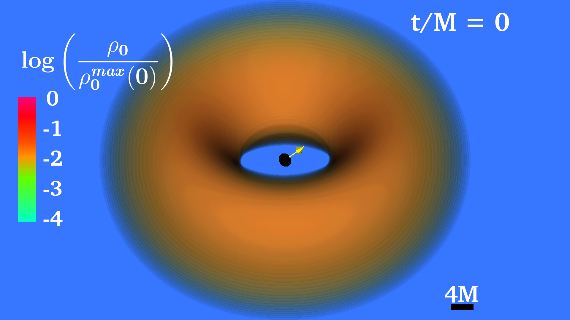
Figure 2: Three dimensional rendering of BHD model A2 at $t=0$. The direction of the BH spin tilted at $45^{\circ}$ with respect to the z axis (axis of the orbital angular momentum of the disk) is shown by the yellow arrow. The black spheroidal region denotes the apparent horizon.

For the Euler equations we assume stationarity and axisymmetry Tsokaros et al. (2019), which is a reasonable assumption whenever the disk is far away from the tilted BH. The density profiles along the x axis for our models are plotted in the top panel of Fig. (1). The disk is described by a $\Gamma=4/3$ polytropic equation of state, having constant specific angular momentum $\ell=-u_{\phi}/u_{t}$. Note that there exist other diagnostics for the specific angular momentum, such as $j=u_{t}u^{\phi}=\ell/(1-\Omega\ell)$, as well as $hu_{\phi}$. Here $h$ is the specific enthalpy, $u_{\phi}$ the azimouthal component of the 4-velocity, and $\Omega=u^{\phi}/u^{t}$ the angular velocity of the fluid. The three diagnostics are plotted in the bottom panel of Fig. (1) for case A1 while similar behavior can be found for cases A2-A4. Our disk models have both $\ell$ and $hu_{\phi}$ constant.

For the numerical solution of the Poisson-type of equations we use the Komatsu-Eriguchi-Hachisu method for BHs, which was first developed in Tsokaros and Uryū (2007). The self-gravitating BHD is calculated as follows: i) First we calculate a massless disk Chakrabarti (1985); Villiers et al. (2003) around a tilted, spinning BH whose mass is $m$ and dimensionless spin is $a/m=0.95$. We call $m$ the BH bare mass. ii) Using as initial data the solution obtained in (i) we iterate over the Einstein and Euler equations to compute a self-gravitating disk of a given maximum rest-mass density. iii) By increasing the maximum density of the disk and repeating step (ii) we compute a sequence of BHDs whose disk mass is growing. For each solution the angular momentum of the BH $J_{\rm bh}$ is calculated through the isolated horizon formalism Ashtekar and Krishnan (2004); Dreyer et al. (2003). Using the apparent horizon finder described in Tsokaros and Uryū (2007) we calculate the mass of the BH $M_{\rm bh}$ Christodoulou (1970), and its dimensionless spin $\chi=J_{\rm bh}/M_{\rm bh}^{2}$. In Fig. 2 a full three-dimensional rendering of the BHD model A2 is shown. The yellow arrow depicts the spin of the BH, which is tilted at $45^{\circ}$ with respect to the z axis. The latter coincides with the axis of rotation of the disk. The apparent horizon is denoted by a black spheroid which is similarly tilted. Models A1, A3, and A4 have similar disk structure, differing mainly on the tilt angle of the BH.

II.1 Precession frequencies

The relevant post-Newtonian (PN) theory for understanding a massive disk around a tilted BH is summarized in Thorne et al. (1986), which we closely follow in the analysis below. In particular we assume a massive thin disk confined on the xy plane having angular momentum $\mathbf{J}_{\rm d}$ along the z-axis, and whose inner radius is $b_{\rm in}$ while its outer radius is $b_{\rm out}$ (see Fig. 3). The disk rotates about a BH having angular momentum $\mathbf{J}_{\rm bh}$ tilted with respect to $\mathbf{J}_{\rm d}$. We further assume that the disk lies outside the BP radius so that it is not driven down to the hole’s equatorial plane (perpendicular to $\mathbf{J}_{\rm bh}$). In our simulations there is no viscosity, so in principle there is no such accretion and no BP effect. Now we imagine that the thin disk is composed of massive rings, each one of them having a mass $dM_{\rm R}$, and radius $b$. The ring’s GM field will make the BH precess around the disk’s rotation axis $d\mathbf{J}_{\rm bh}/dt=\bm{\Omega}_{\rm GM}\times\mathbf{J}_{\rm bh}$ where $\Omega_{\rm GM}=2J_{\rm R}/b^{3}$ and $J_{\rm R}$ the angular momentum of the ring. Generalizing to the disk of Fig. 3 we can write

$$d\Omega_{\rm GM}=\frac{2}{b^{3}}dJ_{\rm R}(b).$$ (2)

If $\sigma(b)$ is the surface gas density and $\omega(b)$ the angular velocity of the ring, we have

$$dJ_{\rm R}(b)=\omega(b)b^{2}dM_{\rm R}=\omega(b)b^{2}(\sigma(b)\;2\pi bdb),$$ (3)

where

$$\sigma(b)=\int_{-h(b)}^{h(b)}\rho_{0}(b,z)dz,\quad\omega(b)=\int_{-h(b)}^{h(b)}\Omega(b,z)dz,$$ (4)

are calculated as quadratures over the disk height $h(b)$ at the particular radius $b$. In Eq. (4) $\rho_{0}(b,z)$ is the rest-mass density of our 3d disks, and $\Omega(b,z)$ their angular velocity profile. Note that although in Newtonian gravity von Zeipel’s theorem von Zeipel (1924) states that for a barotropic fluid the angular velocity of a stationary disk depends only on the distance from the axis of rotation (Poincaré-Wavre Tassoul (1978)), in general relativity the surfaces of constant $\Omega$ have cylindrical topology, therefore they depend not only on the distance from the rotation axis but also on the distance from the equatorial plane Abramowicz (1974); Karkowski et al. (2018).

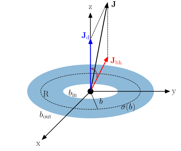
Figure 3: A thin massive disk on the xy plane with angular momentum $\mathbf{J}_{\rm d}$ along the z axis rotates around a tilted spinning BH with angular momentum $\mathbf{J}_{\rm bh}$. Both of them undergo GM precession about the total angular momentum $\mathbf{J}$.

From Eqs. (2)-(4) the GM precession angular velocity of the BH will be

$$\Omega_{\rm GM}=\int_{b_{\rm in}}^{b_{\rm out}}4\pi\omega(b)\sigma(b)db,$$ (5)

where $b_{\rm in}$ and $b_{\rm out}$ are the radial boundaries of the disk. Inserting in Eqs. (4), (5) the density and angular velocity of our tilted self-gravitating disk models A2 and A3 we can compute $\Omega_{\rm GM}$. These theoretical PN estimates are reported in the last column of Table 1 in terms of the GM precession period $P_{\rm GM}=2\pi/\Omega_{\rm GM}$.

Note that a ring of mass $M_{\rm R}$ rotating with Keplerian angular velocity around a BH of mass $M_{\rm bh}$ at a radius $b_{\rm R}$ will be subject to GM precession with

$$M\Omega_{\rm GM}=2\left(\frac{M}{b_{\rm R}}\right)^{5/2}\left(\frac{M_{\rm bh}}{M}\right)^{1/2}\left(\frac{M_{\rm R}}{M}\right),$$ (6)

where $M$ is the ADM mass of the system. For our models $\{$A2, A3$\}$ Eq. (6) yields $P_{\rm GM}/P_{c}=\{54,31\}$ in rough agreement with the values shown in Table 1. This shows that despite the constant specific angular momentum our self-gravitating disks are effectively close to the Keplerian test-ring model.

Not only does the disk makes the BH to precess: conservation of the total angular momentum $\mathbf{J}=\mathbf{J}_{\rm bh}+\mathbf{J}_{\rm d}$ implies that the BH will make the disk precess, i.e.,

$$\frac{d\mathbf{J}_{\rm d}}{dt}=\left(\frac{2\mathbf{J}_{\rm bh}}{b^{3}}\right)\times\mathbf{J}_{\rm d}.$$ (7)

The precession frequency of the disk $\Omega_{\rm GM-disk}$ is related to the precession frequency of the BH $\Omega_{\rm GM}$ as

$$\Omega_{\rm GM-disk}=\Omega_{\rm GM}\frac{J_{\rm bh}}{J_{\rm d}}.$$ (8)

For models A2 and A3 we find that $P_{\rm GM}/P_{\rm GM-disk}$ is of order $1.0$ implying that the spin of the BH will precess at the same timescale as the warping of the disk.

Table 2: Grid parameters used for the evolution of the BHDs of Table 1. The computational grid consists of a set of 13 nested refinement boxes centered on the BH apparent horizon. The step interval in the coarser level is $\Delta x_{\rm max}=50M_{\rm bh}$, while in the finer refinement level is $\Delta x_{\rm min}\approx 0.0122M_{\rm bh}$. Note that the ADM mass $M\approx 1.2M_{\rm bh}-1.3M_{\rm bh}$ depending on the model.

$\{x,y,z\}_{\rm min}$	$\{x,y,z\}_{\rm max}$	Grid hierarchy (Box half-length)
$-4000M_{\rm bh}$	$4000M_{\rm bh}$	$\{0.5,\;1.56,\;3.12,\;6.24,\;12.48,\;25,\;50,\;100,\;200,\;399,\;799,\;1597,\;4000\}M_{\rm bh}$

As a final note we mention that the disk’s tidal field will also exert a torque on the BH that leads to tidally torqued precession with angular velocity Thorne et al. (1986)

$$\Omega_{\rm T}=\frac{3aM_{\rm R}}{2b^{3}_{\rm R}}\cos\theta_{s}.$$ (9)

For model A2 we find $P_{\rm T}/P_{\rm GM}\approx 8$ using $b_{\rm R}$ as the radius of the maximum density. On the other hand we can perform an analysis similar to the GM frequency and write $d\Omega_{\rm T}=3adM_{\rm R}\cos\theta_{s}/(2b^{3})$, with $dM_{\rm R}=\sigma(b)2\pi bdb$. Integrating as in Eq. (5), we find $P_{\rm T}/P_{\rm GM}\approx 9$ in agreement with the cruder estimate above. Therefore the tidally torqued precession is secondary to the GM precession and needs very long evolutions to be probed.

            Tilt: $0^{\circ}$

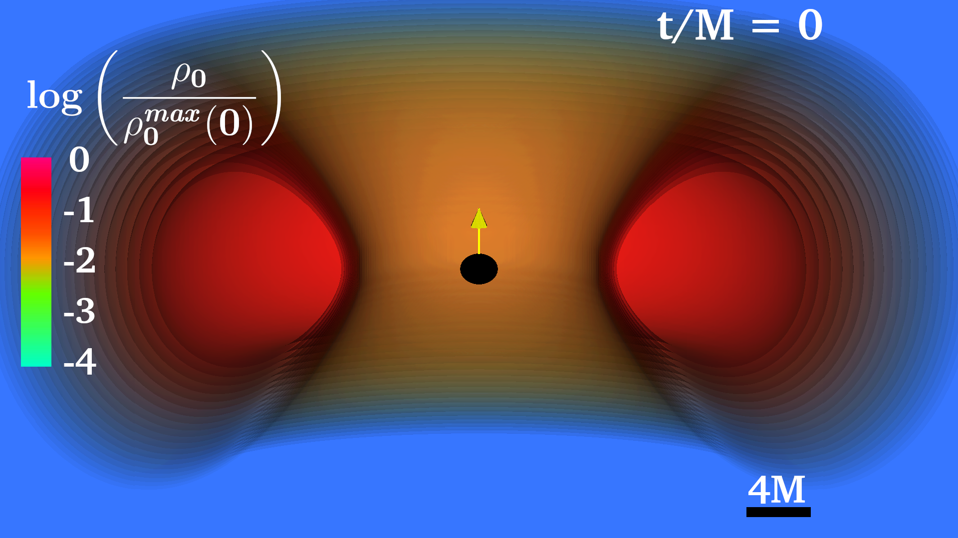
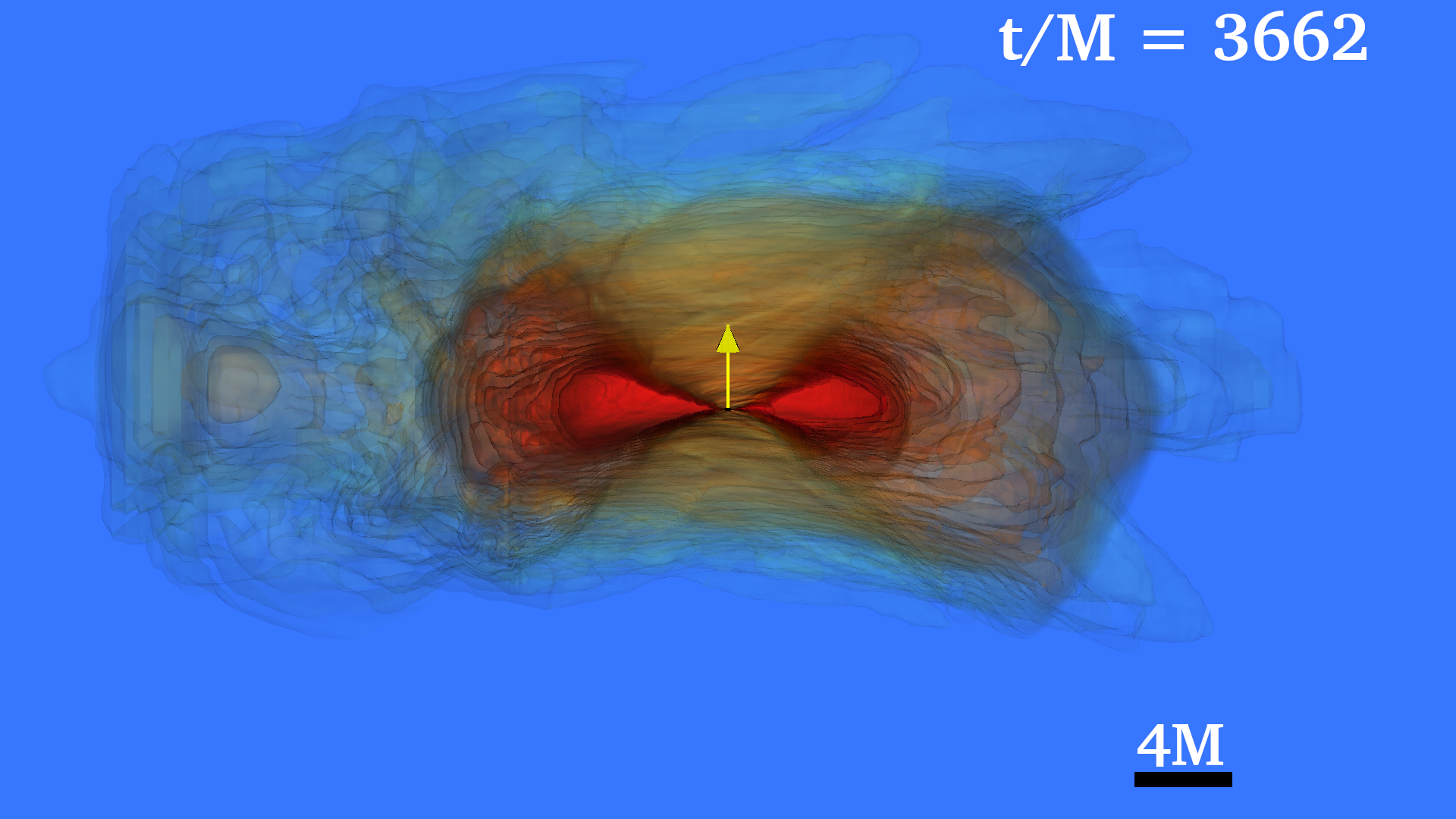
            Tilt: $45^{\circ}$

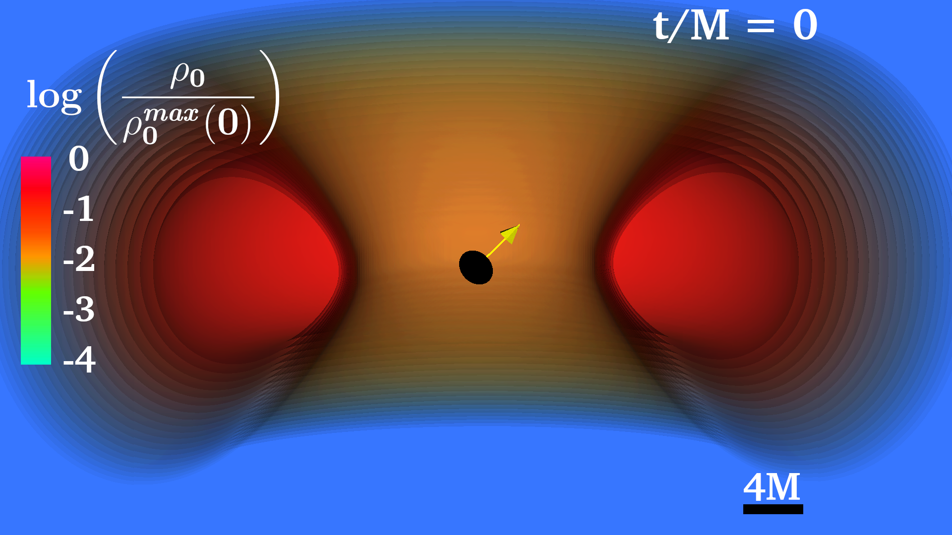
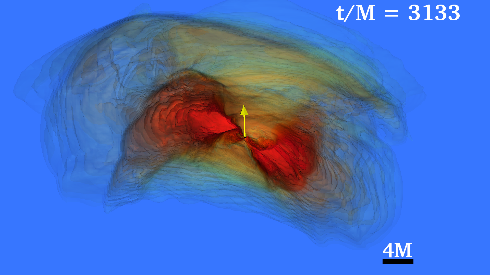
            Tilt: $90^{\circ}$

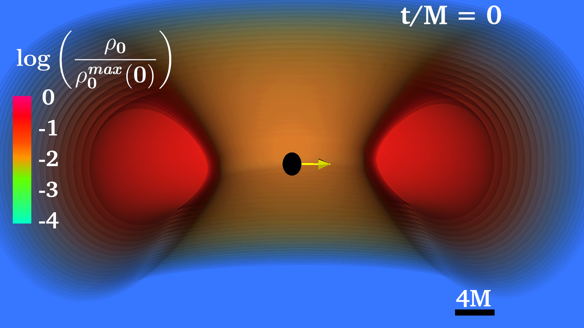
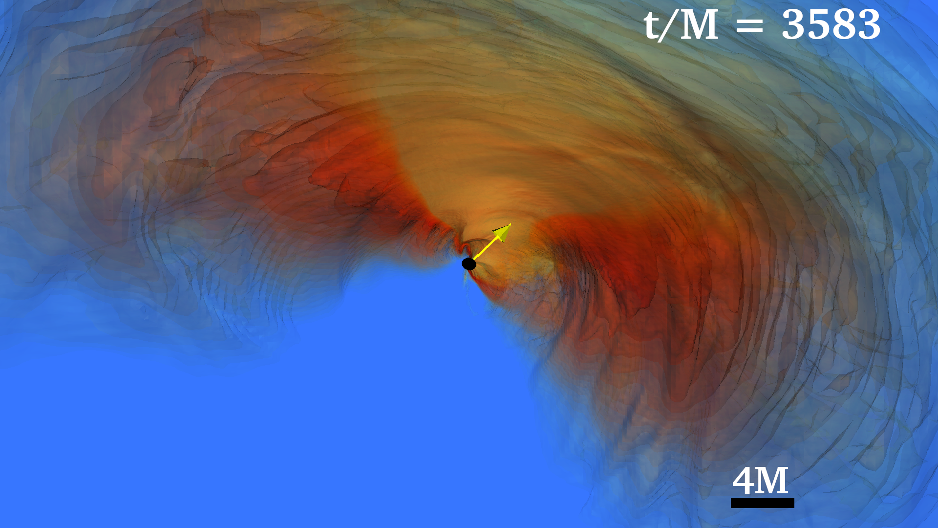
            Tilt: $180^{\circ}$

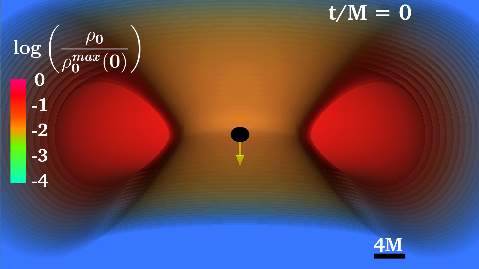
Figure 4: Meridional cuts for the initial (left column) and final (right column) state of the rest-mass density for models A1 (first row), A2 (second row), A3 (third row), and A4 (fourth row). The direction of the BH spin is given by the yellow arrow. The black spheroidal regions denote the apparent horizon.

            Tilt: $0^{\circ}$

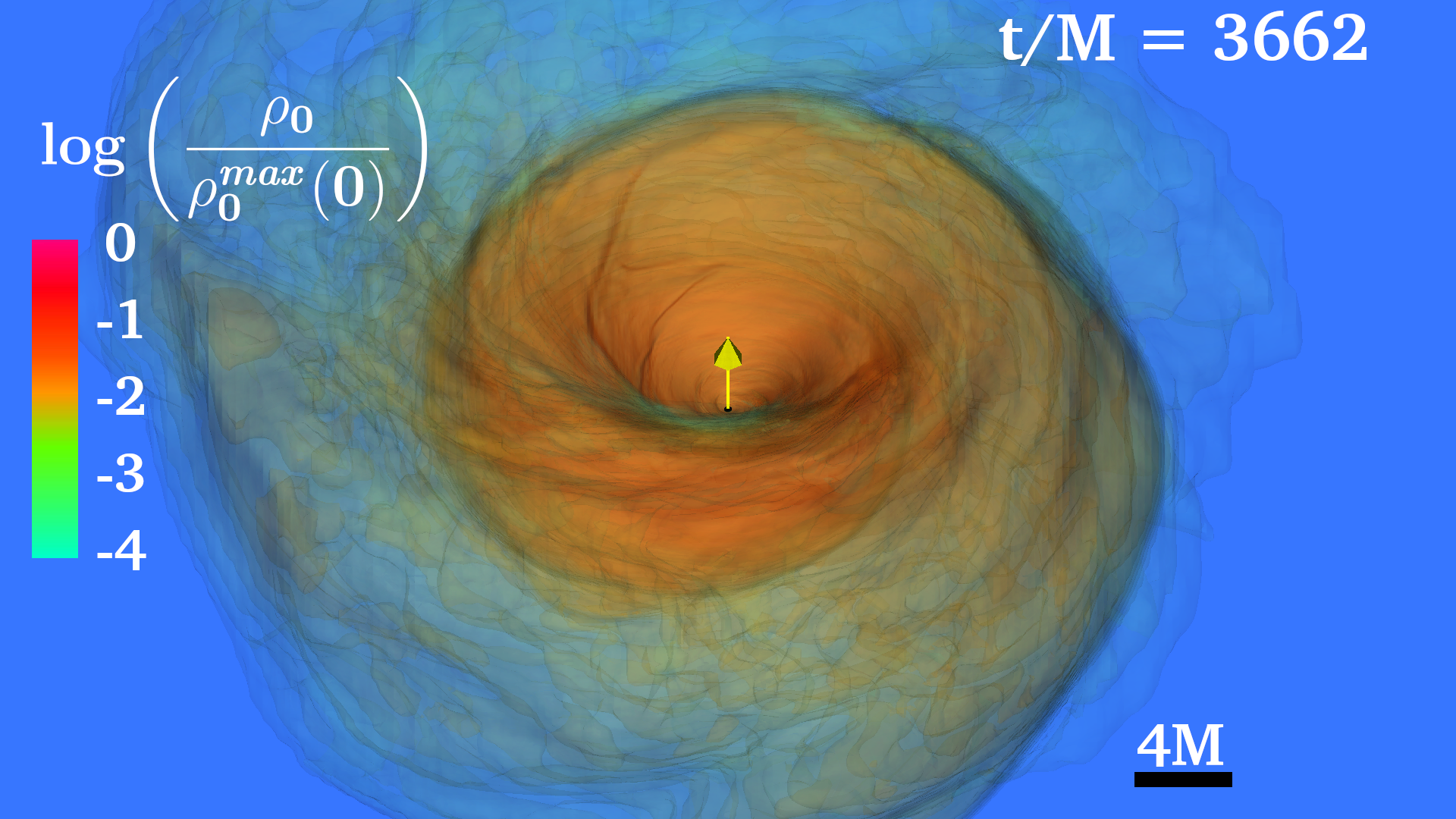
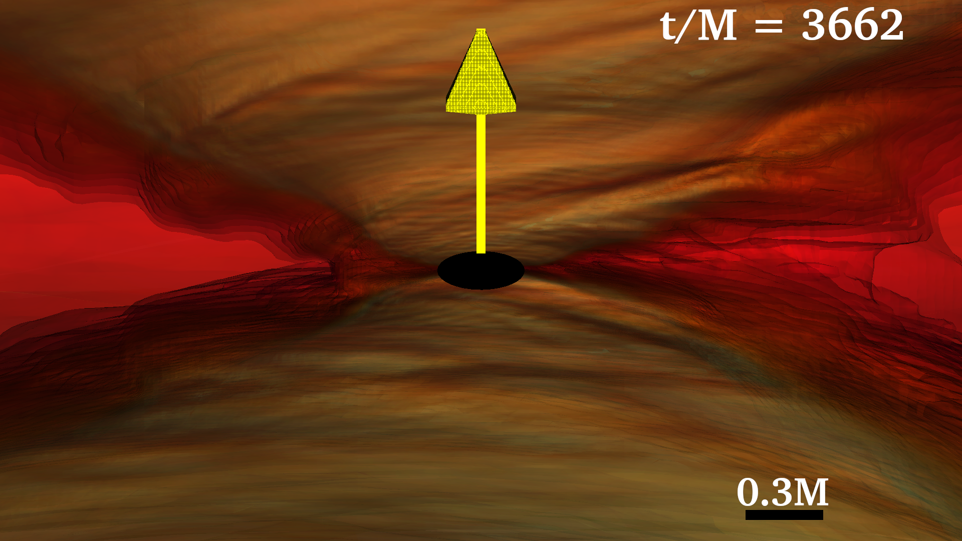
            Tilt: $45^{\circ}$

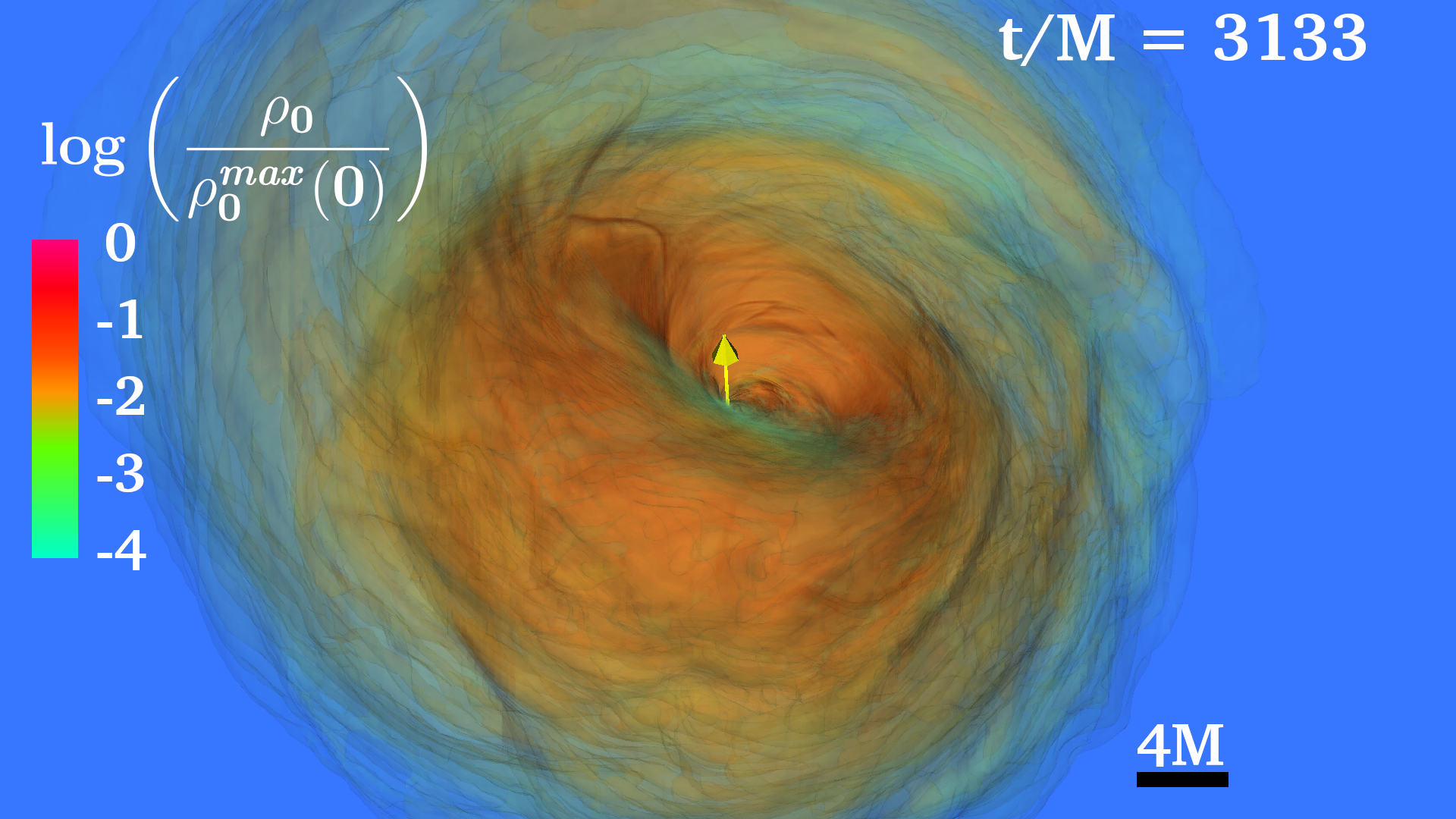
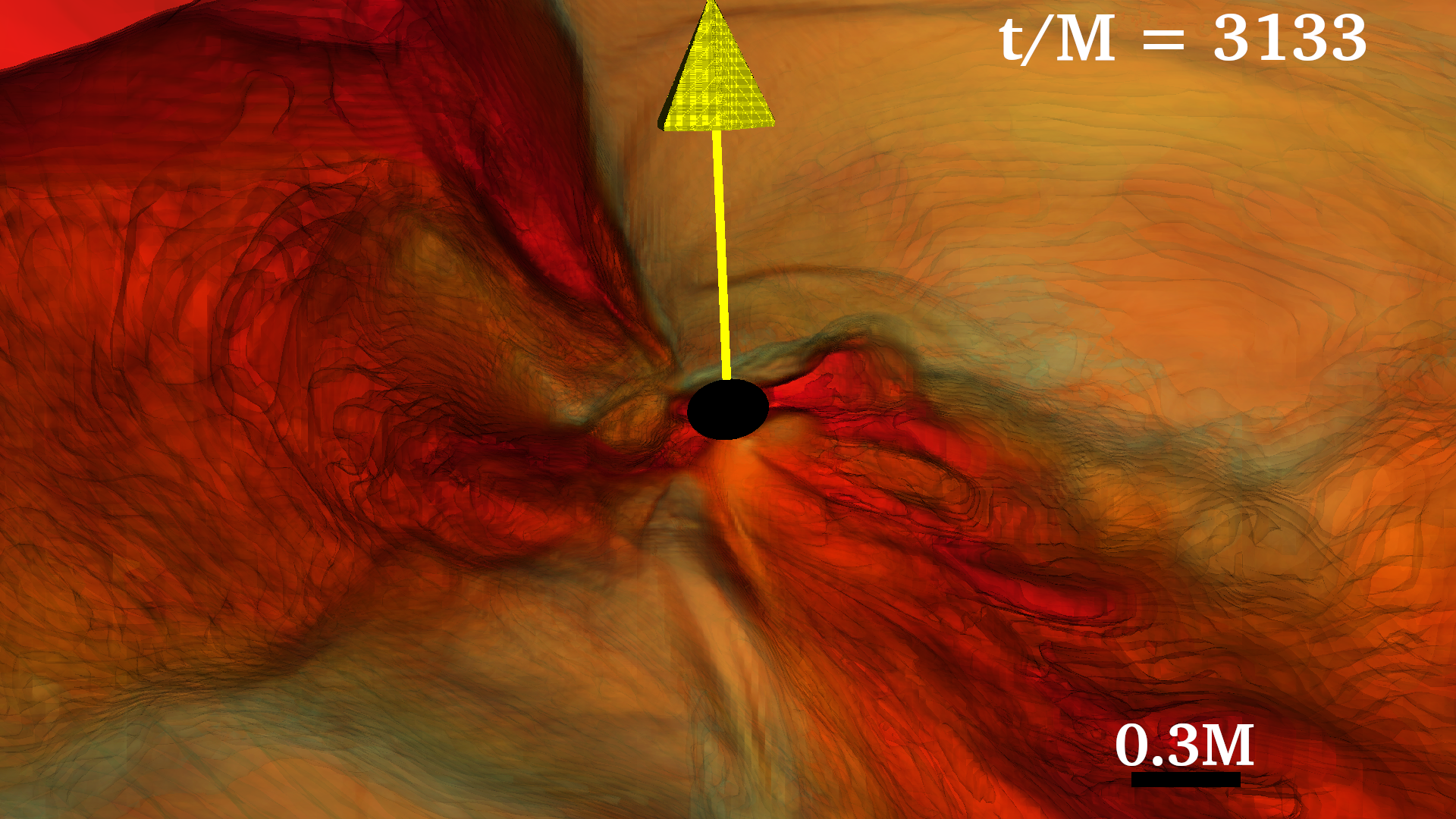
            Tilt: $90^{\circ}$

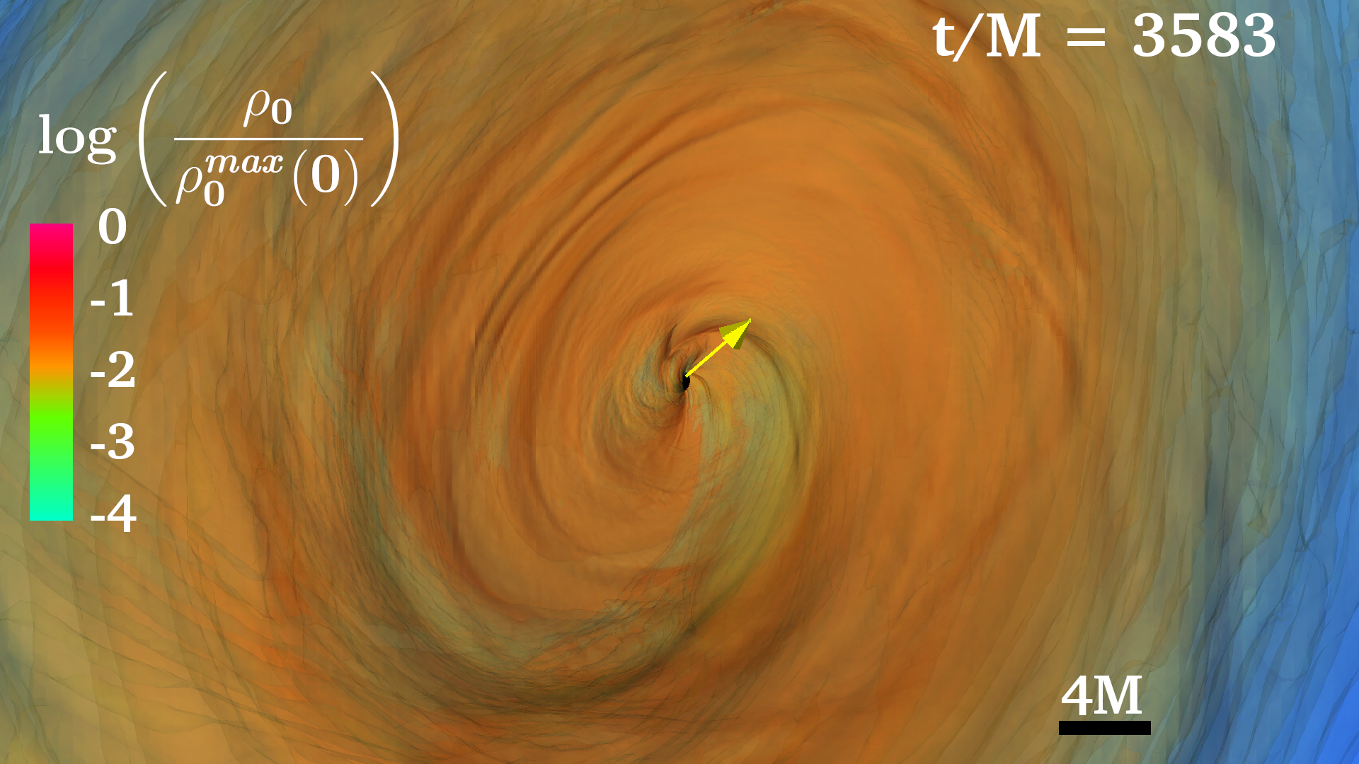
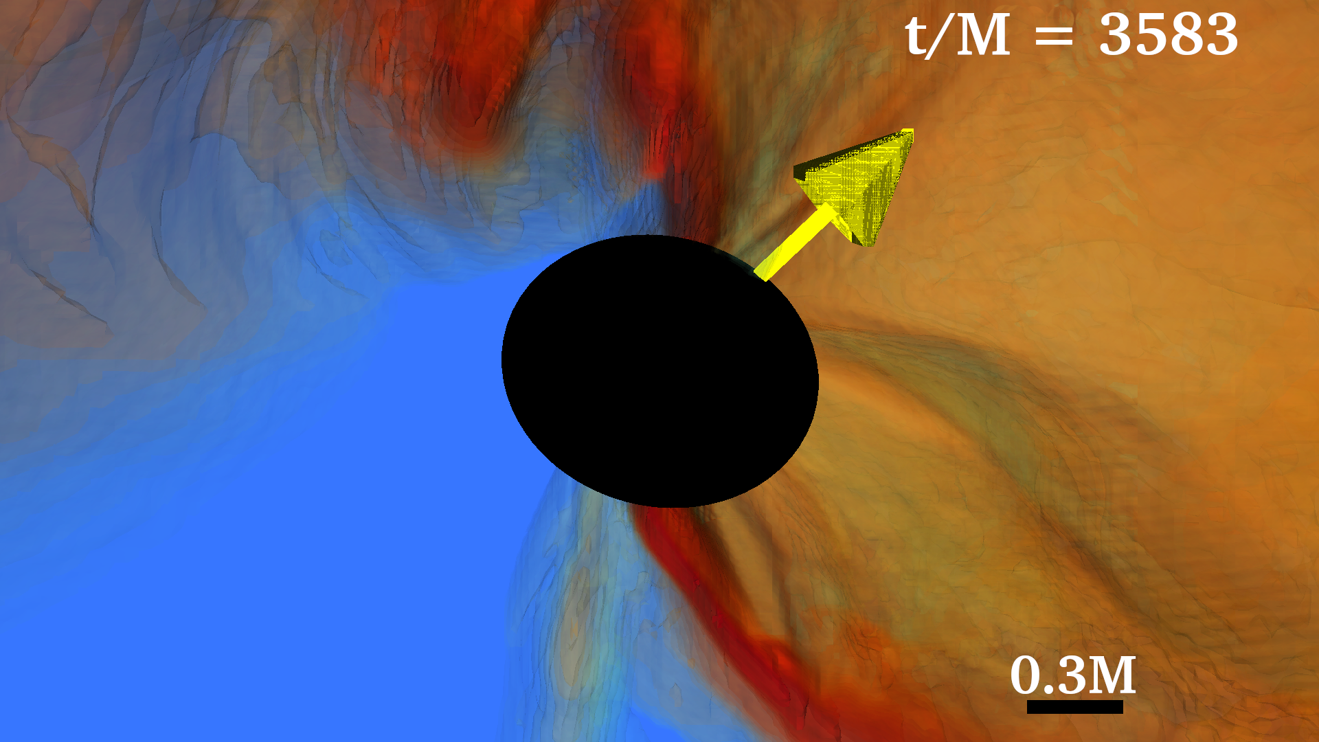
            Tilt: $180^{\circ}$

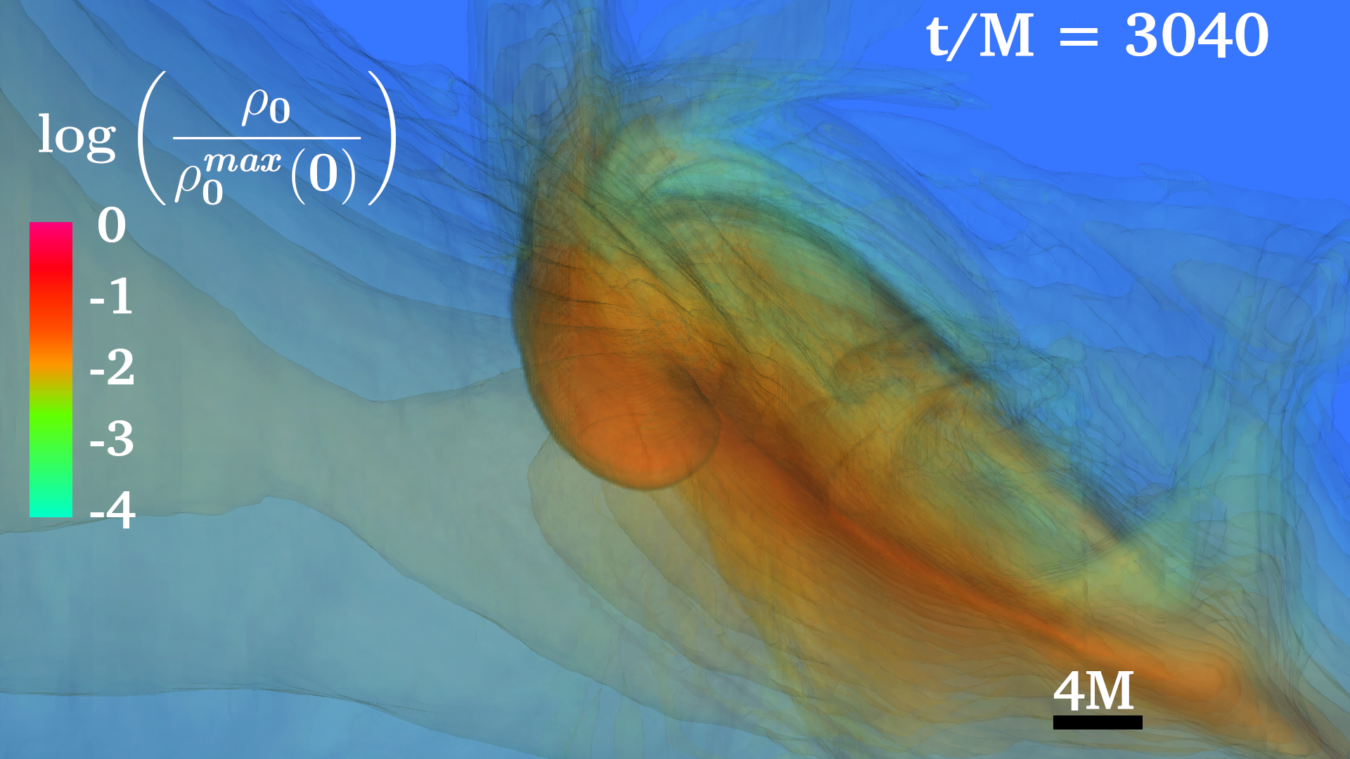
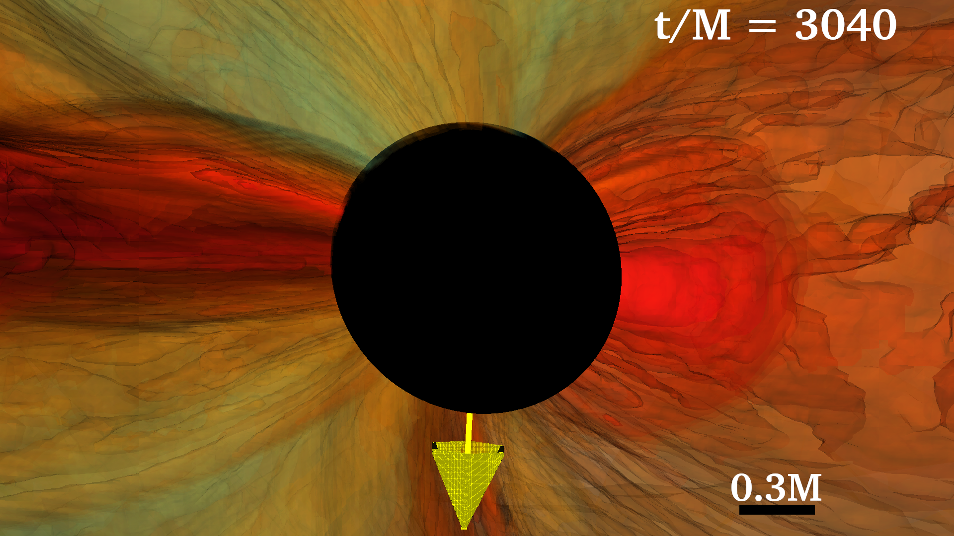
Figure 5: Left column full 3d rendering of the disk rest-mass density at the final moment in our simulations. The right column zooms in near the BH at the same time as the left column. The rest-mass densities are plotted for models A1 (first row), A2 (second row), A3 (third row) and A4 (fourth row). The direction of the BH spin is given by the yellow arrow. The black spheroidal regions denote the apparent horizon.

III Evolutions

The models A1-A4 of self-gravitating BHDs are evolved using the Illinois grmhd moving-mesh-refinement code that employs the Baumgarte–Shapiro–Shibata–Nakamura (BSSN) formulation of the Einstein’s equations Shibata and Nakamura (1995); Baumgarte and Shapiro (1999) to evolve the spacetime fields. Outgoing wave-like boundary conditions are applied to all BSSN variables, which are evolved using the equations of motion (9)-(13) in Etienne et al. (2008), along with the $1+$log time slicing for the lapse $\alpha$, and the “Gamma–freezing” condition for the shift $\beta^{i}$, cast in first-order form (see Eq. (2)-(4) in Etienne et al. (2008)). Time integration is performed via the method of lines using a fourth-order accurate Runge-Kutta integration scheme with a Courant-Friedrichs-Lewy factor set to $0.36048$. Spatial derivatives are computed with fourth-order, centered finite differences, except on shift advection terms, where we employ fourth-order upwind differencing. We use the Carpet infrastructure Schnetter et al. (2004); Carpet to implement moving-box adaptive mesh refinement, and add fifth-order Kreiss-Oliger dissipation Baker et al. (2006) to spacetime and gauge field variables. For numerical stability, we set the damping parameter $\eta$ appearing in the shift condition to $\eta\approx 26.6/M$. For further stability we modify the equation of motion of the conformal factor $\phi$ by adding a constraint-damping term (see Eq. (19) in Duez et al. (2003)) which damps the Hamiltonian constraint. We set the constraint damping parameter to $c_{H}=0.08$ (see also Raithel and Paschalidis (2022)).

High resolution, shock-capturing methods Etienne et al. (2012, 2010) are used for the equations of hydrodynamics, which are written in conservative form. The primitive, hydrodynamic matter variables are the rest-mass density, $\rho_{0}$, the pressure $P$ and the coordinate three velocity $v^{i}=u^{i}/u^{0}$. The stress energy tensor is $T_{\alpha\beta}=\rho_{0}hu_{\alpha}u_{\beta}+Pg_{\alpha\beta}$. For the EOS we use the ideal gas $\Gamma$-law $P=(\Gamma-1)\rho_{0}\epsilon$ with $\Gamma=4/3$, and $\epsilon$ the specific internal energy. The grid hierarchy used in our simulations is summarized in Table 2. It consists of a set of 13 nested mesh refinement boxes centered on the BH apparent horizon. The computational domain is $[-4000M_{\rm bh},4000M_{\rm bh}]^{3}$. The half-side length of the finest box has $\Delta x_{\rm min}=50M_{\rm bh}/2^{12}=0.0122M_{\rm bh}$. Note that the ADM mass is $M\approx 1.2M_{\rm bh}-1.3M_{\rm bh}$ depending on the model. In our simulations we do not assume any symmetry. The extremely high resolution used is necessary in order to capture accurately the dynamics of the highly spinning BHs.

III.1 Global structure

The overall evolution of models A1-A4 can be seen in Figs. 4 and 5. At $t=0$ (left column of Fig. 4) the disks have very similar geometries (see also Fig. 1) while the BHs have the same mass and similar spin magnitudes. Thus the main difference in our cases is the BH tilt angle, which results in distinct behaviors for the 4 models. Note that in Figs. 4 and 5 the magnitude of the BH spin vector is not to scale. Also the shrinkage of the BH and the disk sizes in the right column of Fig. 4, and the left column of Fig. 5 are due to gauge effects arising from differences between the initial data and the evolution gauge choices. On the right column of Fig. 4 we depict a meridional cut at the final moment in our evolutions. For the aligned case (top row) the BH preserves its spin orientiation and magnitude and the disk retains its broad characteristics. The one-arm instability fully develops, but the induced BH orbit remains bounded. On the other hand, the antialigned case (bottom row) after a certain time becomes largely unstable, with the disk losing its initial structure and exhibiting massive mass accretion. The BH acquires a kick velocity that results in an unbound orbit (keeps drifting away until the end of our simulations). Although the BH spin orientiation is preserved, its magnitude is significantly reduced due to accretion.

For the misaligned cases (second and third rows), we observe the combined effects of (i) BH precession, (ii) disk precession and warping around the BH, (iii) development of the PPI, (iv) acquisition of a small BH kick velocity, (v) significant gravitational wave emission of various modes beyond the $\ell=2$, $m=2$ which are as strong as the $(2,2)$ mode, and (vi) in the A3 case ($90^{\circ}$ initial tilt), we observe an overall broad alignment of the disk with the BH spin (third row in Fig. 4, right column). This alignment is not associated with the BP effect, which requires a viscosity mechanism absent in our simulations. In addition, the alignment in our case is global, i.e. the whole disk rotates like a solid body, instead of the alignment of only the inner regions of the disk typical of the BP picture. In fact, from the third row, right column of Fig. 5, where the two streams onto the BH are apparent, we confirm that there is no such alignment in the inner regions of the disk. Our results are reminiscent of the behavior described in Fragile and Anninos (2005); Fragile et al. (2007) and referred as “plunging streams”. The additional complication in our case though is that the BH-disk spacetime is dynamical and responds to the motion of the disk. As in Fragile and Anninos (2005); Fragile et al. (2007) the plunging streams enter the BH above and below its symmetry plane from almost antipodal points due to strong differential precession and the nonspherical nature of the spacetime. For a Kerr BH (which is very close to the BHD spacetimes close to the horizon) orbital stability strongly depends on the inclination of the orbit, with the unstable region being larger for increasing inclination. Also the value of $r_{\rm ISCO}$ is larger for larger inclinations Hughes (2001); Fragile et al. (2007). For the A3 case we observe the largest BH kick velocity which is $\sim 2\ \rm km/s$. For model A2 ($45^{\circ}$ initial tilt angle) we could not evolve beyond $t\approx 3133M$ because the BH was spun up to maximal spin. At that point both the BH and the disk experience a tilt by $\sim 45^{\circ}$ with respect to their initial orientation, but in opposite directions (see second row, right column in Fig. 4) Similar to case A3 and Fragile and Anninos (2005); Fragile et al. (2007), we observe two plunging streams in opposite directions entering the BH above and below its symmetry plane. The warping of the disk around the BH for both cases A2 and A3 is significant (see Fig. 5 second and third row).

Table 3: Mode growth, pattern speed, and corotating radius for the $m=1$ mode.

Model	${\rm Im}(\omega_{1})/\Omega_{c}$	$\Omega_{p,1}/\Omega_{c}$	$r_{\rm cr}/r_{\rm c}$
A1	$0.318$	$0.748$	$1.17$
A2	$0.177$	$0.748$	$1.17$
A3	$0.177$	$0.637$	$1.24$
A4	$0.227$	$0.812$	$1.12$

III.2 Mode growth and angular momentum transport

According to previous studies, both Newtonian and general relativistic, we expect all our models to be dynamically unstable to the one-arm ($m=1$) spiral-shape instability. In the general relativistic simulations of Korobkin et al. (2011); Mewes et al. (2016, 2016) it was concluded that if the mass of the disk is larger than $\gtrsim 4\%$ of the mass of the BH a fixed background spacetime cannot fully capture the dynamics of the system. In particular in order to accurately describe the dynamical gravitational interaction between a time varying BH (in position, mass and spin), as well as a time varying massive disk, simulations in a non-fixed background spacetime are necessary, as we perform here.

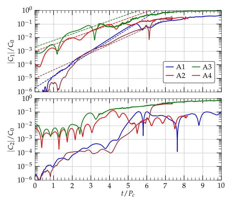
Figure 6: Growth of the $m=1$ (top panel) and the $m=2$ (bottom panel) modes.

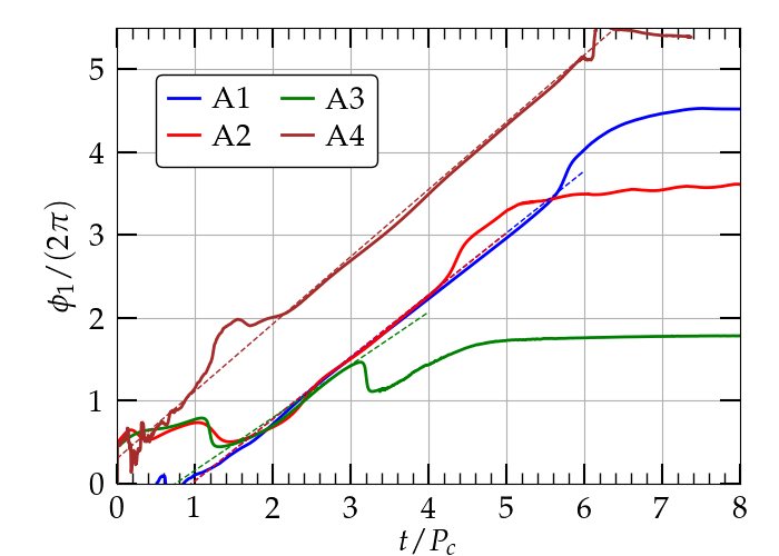
Figure 7: Phase angle $\phi_{1}$ of the mode $m=1$ for models A1-A4.

To quantify the growth of various unstable density modes we evaluate the parameters Paschalidis et al. (2015a); Wessel et al. (2021)

$$C_{m}=\int_{r>r_{\rm ah}}\rho_{0}u^{t}\sqrt{-g}e^{im\phi}d^{3}x,$$ (10)

where $g$ is the determinant of the spacetime metric and $\phi=\tan^{-1}(y/x)$ the azimuthal angle. The volume integral is performed outside the apparent horizon of the BH and the mode amplitude is denoted by the normalized quantity $C_{m}/C_{0}$, where $C_{0}=M_{0}$ the rest mass of the disk. The pattern speed of an azimuthal mode $m$ is defined as Williams and Tohline (1987); Woodward et al. (1994)

$$\Omega_{p,m}=\frac{1}{m}\frac{d\phi_{m}}{dt},$$ (11)

with the phase angle $\phi_{m}$ being

$$\phi_{m}=\tan^{-1}\left(\frac{{\rm Im}(C_{m})}{{\rm Re}(C_{m})}\right).$$ (12)

In other words the pattern speed of any mode is proportional to the slope of the curve $\phi_{m}(t)$ with the proportionality constant being $1/m$.

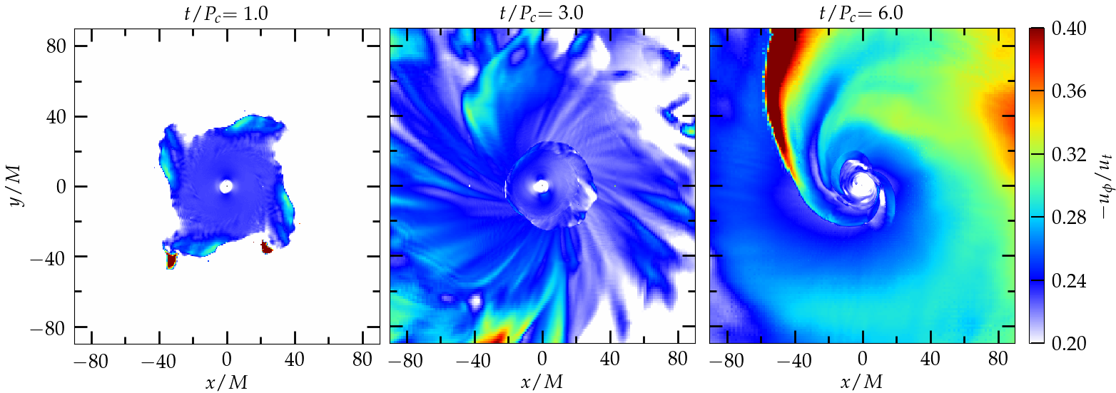
Figure 8: Snapshots at three different times of the specific angular momentum $\ell=-u_{\phi}/u_{t}$ for case A2. To convert to $t/M$ multiply by $373$ (see Table 1).

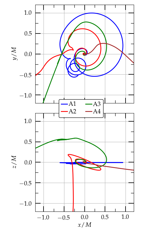
Figure 9: BH trajectory on the xy and xz planes.

As we discussed in the Introduction, the PPI manifests itself when a perturbation which is traveling backwards relative to the fluid at the inner edge, and therefore has $\Omega_{p,m}<\Omega$, exchanges energy and angular momentum with a perturbation which is traveling forwards relative to the fluid at the outer edge and therefore has $\Omega_{p,m}>\Omega$. The radius $r_{\rm cr}$ where the interaction happens is called the corotation radius and satisfies $\Omega_{p,m}=\Omega(r_{\rm cr})$.

In Fig. 6 we plot the $m=1$ (top panel) and $m=2$ (bottom panel) mode growths for all cases A1 (aligned, blue line), A2 ($45^{\circ}$ red line) A3 ($90^{\circ}$ green line), and A4 ($180^{\circ}$ brown line). The most prominent feature of this plot is the fact that for both modes, $(C_{m}/C_{0})(t=0)$ for the tilted cases (A2, A3) are much larger than the ones of A1, A4. In fact for models A2 and A3 $(C_{2}/C_{0})(t=0)\sim O(10^{-2})$ is ten to a hundred times larger than $(C_{1}/C_{0})(t=0)$ and initially slightly decreases while the latter steadily grows in an exponential manner. When $C_{1}/C_{0}$ reaches values $\sim O(10^{-2})$ then the $m=2$ mode grows in a similar manner. In other words the $m=1$ mode drives the growth of the $m=2$, something that is also seen in the aligned and antialigned cases (A1, A4). The fact that in the tilted cases at $t=0$ the $m=1$ mode amplitude is already nonzero and much larger than in the aligned or antialigned cases results in a smaller $m=1$ growth timescale, as can been seen from the slope of the fitted dashed lines (in the top panel of Fig. 6). These timescales are reported in Table 3 second column and are in broad agreement with other studies Korobkin et al. (2011); Wessel et al. (2021). If we denote the growth of the $m=1$ mode as $e^{t/\tau}$, we find that $\tau/P_{c}=\{0.5,0.9,0.9,0.7\}$ for cases A1-A4, confirming that the instability is indeed dynamical. The two tilted cases show almost identical growth timescales, even though the disk in case A3 has almost double the mass of the disk in case A2 while their radial extent is approximately the same. Note that in Kiuchi et al. (2011); Shibata et al. (2021a) it was found that more compact (or more massive) disks are more subject to the dynamical instability, and when $M_{0}/M_{\rm bh}\gtrsim 0.6$ the growth timescale can be smaller than $P_{c}$. Our models show that timescales $\lesssim P_{c}$ are possible with even less massive disks with $M_{0}/M_{\rm bh}\sim 0.16$. This result is not surprising Goldreich et al. (1986) since our disk models have $\ell=\rm const$ which makes them more prone to the development of the PPI than the models of Kiuchi et al. (2011); Shibata et al. (2021a), which have an nonconstant specific angular momentum profile. Given the fact that models A2 and A3 have the same spin magnitude we conclude that the spin tilt is crucial for the determination of the growth timescale and can be degenerate with the BH-to-disk mass ratio.

The phase angle of the $m=1$ mode is shown in Fig. 7 and the slopes of the fitted dashed lines (Eq. (11)) provide the corresponding pattern velocities $\Omega_{p,1}$ that are quoted on Table 3. From this figure one can read easily the time for the saturation of the PPI. In particular for case A1 it is $\approx 5.5P_{c}$, for A2 it is $\approx 4P_{c}$, for A3 it is $\approx 3P_{c}$, and for A4 it is $\approx 6P_{c}$. These values are in agreement with the top panel of Fig. 6 and show that the larger the tilt, the smaller the timespan for the development of the nonaxisymmetric instability. After this initial period, the mode growth saturates and the phase angle $\phi_{1}$ asymptotes to a constant. Interestingly, the $m=1$ pattern speed is almost identical for the cases A1 and A2 despite the different spin orientiations of the BHs, as well as the different BH to disk mass ratios. This may be related to the fact that those models have identical inner $r_{\rm in}$ and outer $r_{\rm out}$ boundaries, which play a crucial role for the explanation of the PPI Papaloizou and Pringle (1984, 1985); Zurek and Benz (1986); Blaes and Glatzel (1986).

Another critical component of the PPI is the corotation radius $r_{\rm cr}$ through which angular momentum is transferred outwards Papaloizou and Pringle (1984); Goldreich et al. (1986); Zurek and Benz (1986); Hawley (1991). In Table 3 we report the ratio of the corotation radius to the radius of the maximum density for our models A1-A4. This ratio is close to unity, which is typical of the $m=1$ PPI mode Korobkin et al. (2011); Mewes et al. (2016, 2016). In terms of the total mass of the system the corotation radii are $r_{\rm cr}/M=\{16,17,17,17\}$. In order to confirm and better understand the development of the PPI in thick, tilted self-gravitating BHDs we plot in Fig. 8 the specific angular momentum $\ell=-u_{\phi}/u_{t}$ at three different instances for case A2. At one rotation period (left panel) the disk has essentially the angular momentum profile of the initial data i.e. $\ell=\rm const$. After three rotation periods (middle panel), when the PPI has been well developed, we see two characteristics: (i) a shock front located at approximately $r\sim 20M$, and (ii) the shock front separating the inner part ($r\lesssim 20M$) of the disk with angular momentum regions having values smaller than the initial angular momentum (white-blue areas) from the outer part ($r\gtrsim 20M$) of the disk with angular momentum regions having values larger than the initial angular momentum (green-yellow-red areas). Also, a spiral structure in the outer part starts to form. After six rotation periods (right panel), where the PPI is fully developed, this picture is even clearer and the characteristic spiral arm is apparent. This shows how the PPI can redistribute angular momentum by outward transport.

The growth of the one-arm instability results in a pseuso-binary system consisting of the BH and the $m=1$ “planet” that sets the BH in motion. In Fig. 9 we depict the trajectory of the BH in the equatorial (top panel) and meridional (bottom panel) planes. In all cases we notice the characteristic spiral trajectory resulting from the spiral motion of matter in the disk (see Fig. 5 left column and Fig. 8) and the conservation of the center of mass of the system. For case A1 the motion is planar (in the xy plane) with larger radius of curvature in the beginning when the PPI develops and smaller at the end, when it has saturated. For the tilted cases A2 and A3 this motion is three dimensional, while for the antialigned case A4 we again have a three-dimensional motion due to the destabilization of the whole system after $\sim 6$ rotation periods. The evolution of A4 will be further described in the next section. The combined motion of the BH with the self-gravitating disk produces copious amounts of gravitational radiation, as we will discuss next.

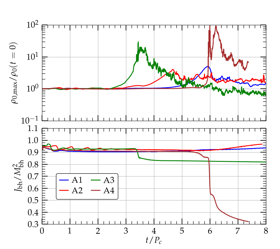
Figure 10: Evolution of the maximum rest-mass density of the disk (top panel) and the BH dimensionless spin (bottom panel).

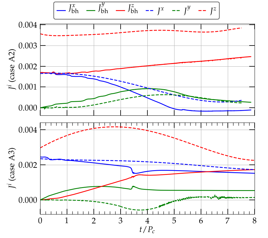
Figure 11: Evolution of the BH (solid lines) and ADM (dashed lines) angular momentum components for the tilted cases A2 ($45^{\circ}$) and A3 ($90^{\circ}$).

III.3 Precession and gravitational waves

In the top panel of Fig. 10 we plot the evolution of the maximum density in the disk. The general trend shows the maximum density to be constant until approximately the end of the development of the PPI, at which point nonlinear growth sets in and can lead to an increase of $\rho_{0,\rm max}$ by orders of magnitude. Consistent with Figs. 6 and 7 we observe the peak of $\rho_{0,\rm max}$ for case A1 to happen at $\sim 6P_{c}$ which coincides with the end of the linear growth of the phase angle $\phi_{1}$ in Fig. 7. Similarly for the cases A2, A3, and A4 the peak times are $\sim\{4.5P_{c},3.5P_{c},6P_{c}\}$. Depending on the characteristics of the system the maximum density relaxes to values higher or lower than the initial maximum density and leads to persistent emission of gravitational waves. Also, as already discussed, the larger the tilt, the earlier the peak of the maximum density.

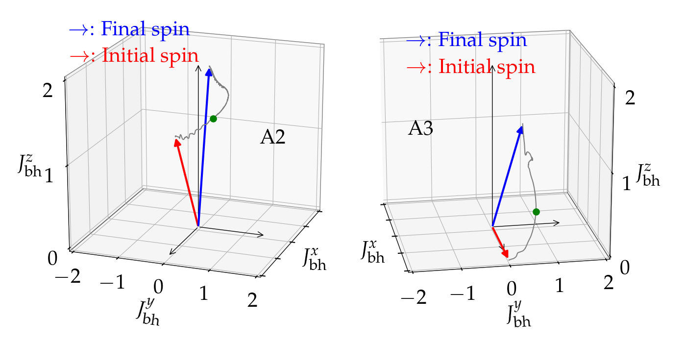
Figure 12: BH spin precession for the two tilded cases A2 and A3. The magnitude of the spin vector is not in scale. The gray curve shows the evolution of the spin from its initial value (red arrow) to its final value (blue arrow). Green dots denote times $t=3P_{c}$ for model A2, and $t=2P_{c}$ for model A3.

In the bottom panel of Fig. 10 the dimensionless spin parameter $\chi=J_{\rm bh}/M_{\rm bh}^{2}$ is plotted as a function of time for all our models. We adopt the AHFinderDirect thorn Thornburg (2004) to locate and monitor the apparent horizon, and the isolated horizon formalism Dreyer et al. (2003) to measure the mass of the BH, $M_{\rm bh}$, and its dimensionless spin parameter $\chi$. For the cases A1, A4, we have also confirmed that the Kerr formula for the ratio of proper polar horizon circumference $L_{p}$, to the equatorial one $L_{e}$, $L_{p}/L_{e}=4\sqrt{r_{+}^{2}+a^{2}}\ E\left(\frac{a^{2}}{r_{+}^{2}+a^{2}}\right)$ (here $E(x)$ is the complete elliptic integral of the second kind, $r_{+}$ the event horizon in Boyer-Linquist coordinates, and $a=J_{\rm bh}/M_{\rm bh}$ the Kerr spin parameter), and its approximation $L_{p}/L_{e}\approx(\sqrt{1-(a/M_{\rm bh})^{2}}+1.55)/2.55$ Brandt and Seidel (1995), yields almost identical results for the evolution of $\chi$. For the tilted case A2 we observe that the BH is spun up and approaches maximum spin, which prevented us to continue the simulation beyond $\sim 8$ rotation periods. For the $90^{\circ}$ tilted case A3 we observe that when the maximum density peaks at $\sim 3.5P_{c}$ significant accretion onto the BH is initiated, which results in a reduction of the rest mass of the disk. At the same time the mass of the BH increases, which leads to an abrupt decrease of its dimensionless spin to $\chi\sim 0.85$. By the end of our simulation at $\sim 8P_{c}$ the disk has $75\%$ of its initial mass and the spin of the BH asymptotes to $\chi\sim 0.82$. The most unstable case in our simulations is the antialigned case A4. At 6 rotation periods the maximum rest-mass density increases by two orders of magnitude and shortly afterwards massive accretion is initiated. That increases the BH mass significantly and its spin drops to $\sim 0.5$. Interestingly, the x and y spin components do not show any appreciable change (i.e. they remain zero), only the z component reduces in magnitude. We didn’t observe such instability in Wessel et al. (2021) where a model with a much smaller spin $\chi=-0.7$ was employed. We plan to investigate this issue in the future. The evolution of the three components of the BH spin as well as the three components of the ADM angular momentum for the two tilted cases A2 and A3 are plotted in Fig. 11. In Fig. 12 we plot the BH spin for the tilted models A2 and A3 as it evolves from its initial value (red arrow) to its final one (blue arrow). The gray curve shows the path of the BH spin vector along our simulations. In order to verify that precession is observed and measured well before significant accretion arises, and to measure accurately the GM-induced precession we show a green bullet that corresponds to $t=3P_{c}$ for model A2 and $t=2P_{c}$ for model A3. Although at those times the PPI is growing (see Figs. 6 and 7) the rest masses of the disks are essentially the same as their initial values. The precession of the BH spin from its initial value (red arrows) to the green bullets is thus mainly due to the GM effect. Projecting the gray path onto the x-y plane and computing its radius of curvature we find that the angle between the projections of the initial spin vector and the spin vector corresponding to the green bullet is $\approx 18^{\circ}$ or $P_{\rm GM}/20$, which yields $P_{\rm GM}\approx 60P_{c}$. This value exactly matches the estimate from the analysis of Section II.1 reported in Table 1. A similar calculation for model A3 yields an angle between the projections of the initial spin vector and the spin vector corresponding to the green bullet of $\approx 19^{\circ}$ or $P_{\rm GM}/19$. Hence $P_{\rm GM}\approx 38P_{c}$ which is in excellent agreement with the estimate reported in Table 1. Therefore our simulations are in agreement with the estimates from the PN analysis in Section II.1.

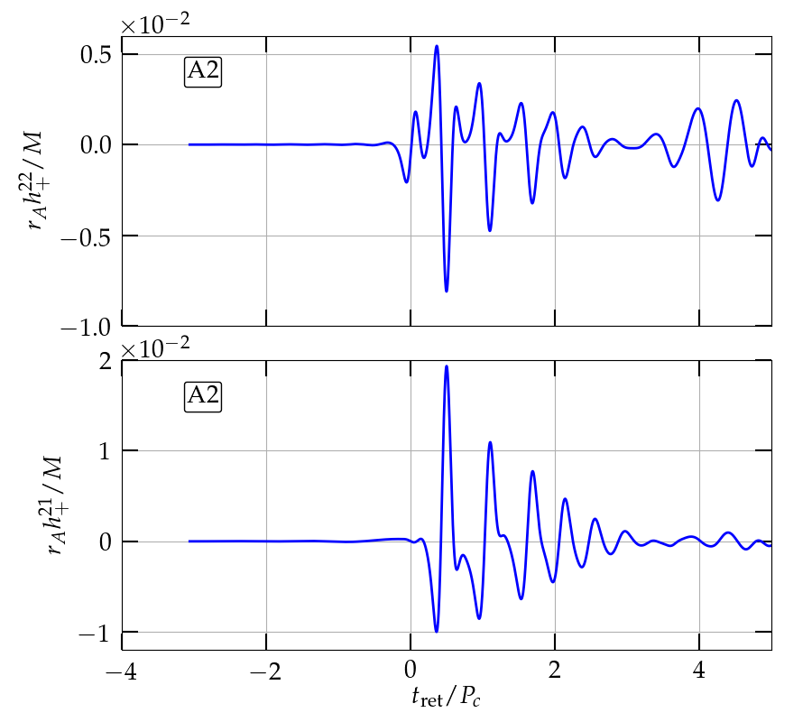
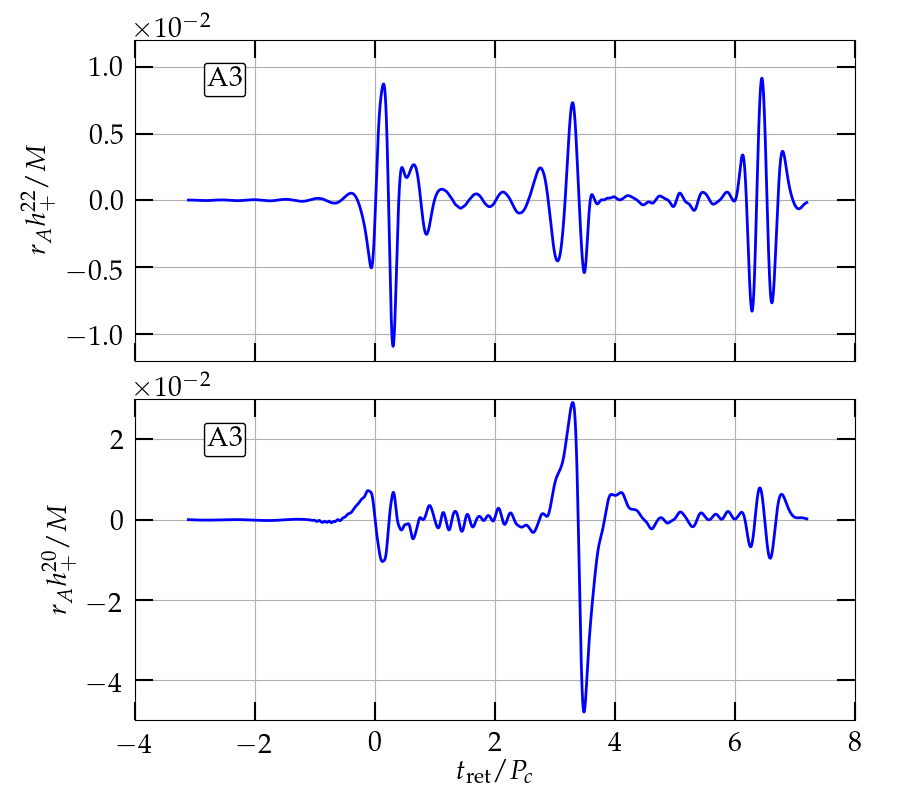
Figure 13: Strain amplitude ($h_{+}$) for various gravitational wave modes for the two tilted models A2 and A3. Here $r_{A}$ is the areal extraction radius and $t_{\rm ret}$ is retarded time.

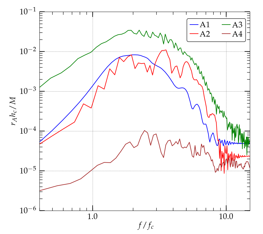
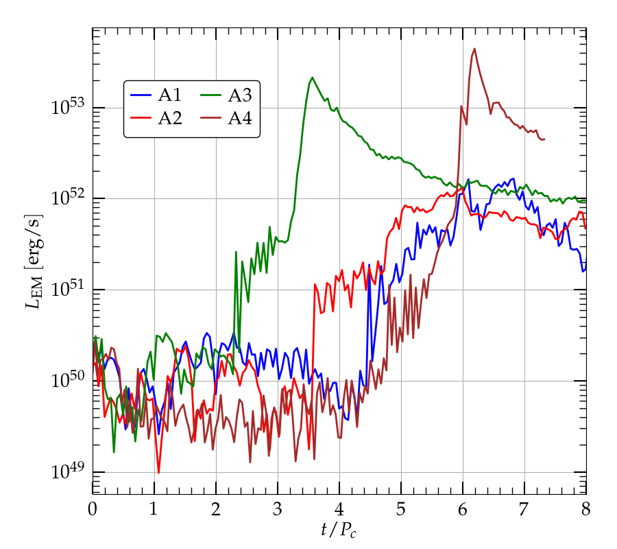
Figure 14: Left panel: Gravitational wave spectrum of the $(2,2)$ mode. Right panel: Estimated bolometric luminosities.

III.4 Multimessenger astronomy

BHDs are prominent sources of electromagnetic radiation due to accretion. In our case because of the self-gravity of the disk such systems also produce significant amounts of gravitational radiation, which makes them excellent sources for multimessenger astronomy. For the extraction of gravitational waves we measure the outgoing component of the complex Weyl scalar $\Psi_{4}$ expanded in terms of the spin-weighted spherical harmonics with spin weight $-2$. at various finite radii. The axis of the spherical harmonics is taken to be the z-axis which is the initial direction of the disk angular momentum. The strain $h$ is then computed with a double integration in time as described in Reisswig and Pollney (2011).

In previous studies Kiuchi et al. (2011); Mewes et al. (2016); Wessel et al. (2021); Shibata et al. (2021a), where nonspinning or aligned BHD systems were analyzed, it was found that the development and saturation of the PPI leads to an initial wave burst, and then a relaxation to a persistent quasimonochromatic signal of lower amplitude. The peak amplitude of the strain depends on the disk-to-BH mass ratio as well as the disk characteristics. Disks of constant specific angular momentum profiles develop a more pronouced $m=1$ instability, thus the amplitude of gravitational wave is larger. As explained in Lai et al. (1994); Wessel et al. (2021) it is $rh\sim O((r_{c}\Omega_{c})^{2})$ and therefore the amplitude of the strain is directly related to the angular velocity and radius of the maximum density point.

When the orbital angular momentum and the BH spin are misaligned this will cause the precession of the orbit and a modulation of the gravitational waves. As we have seen in Section II.1, the angular velocity of the orbital precession is much smaller than the orbital angular velocity, which implies that we will need many rotation periods to observe the imprint of precession on the gravitational waves. In the left column of Fig. 13 we plot the $(2,2)$ mode (top panel) and $(2,1)$ mode (bottom panel) of $h_{+}$ for the tilted case A2 ($r_{A}$ is the areal extraction radius). As we discussed above we could not evolve this model beyond 8 rotation periods due to the almost extremal spin the BH acquires from accretion. Despite that we observe that the initial amplitude of the strain is much larger than in the aligned cases (see for example Wessel et al. (2021)). In this particular model the $(2,1)$ mode has a larger initial amplitude than the $(2,2)$ mode. The reason for this large initial amplitude is not due to the $r_{c}\Omega_{c}$ value mentioned above but from the large nonaxisymmetry of the system at $t=0$. Indeed, the aligned model A1 has the same $r_{c}\Omega_{c}$ value as model A2 but it has a much smaller peak strain even though the rest mass of the disk is larger.

Similar large amplitudes are found on the right panels of Fig. 13 where the $h_{+}$ strain of the modes $(2,2)$ and $(2,0)$ are plotted for the tilted case A3. The large peak of the $(2,0)$ mode is also present in the $(2,1)$ mode, characteristic of mode mixing. Contrary to the A2 case where the $\ell=3$ modes are negligible, case A3 has significant amplitude $\ell=3$ modes. In Mewes et al. (2016) where spins up to $\chi\sim 0.5$ and tilt angles up to $\sim 30^{\circ}$ were employed it was found that the gravitational wave signal has a weak dependence on the initial tilt angle, especially for disks with nonconstant specific angular momentum profiles. The authors observed the smallest peak amplitudes for the most tilted BH spacetime. By contrast, in our simulations we see that the gravitational wave signal can be greatly influenced by the tilt angle as discussed above for the cases A2 and A3. Also, for case A3, which has the largest tilt we observe the largest peak amplitude.

We compute the Fourier power spectrum of the gravitational waves for the $(2,2)$ mode by calculating

$$\tilde{h}(f)=\sqrt{\frac{|\tilde{h}^{22}_{+}(f)|^{2}+|\tilde{h}^{22}_{\times}(f)|^{2}}{2}}.$$ (13)

Here $\tilde{h}^{22}_{+}(f)$ and $\tilde{h}^{22}_{\times}(f)$ are the Fourier transforms of the two independent polarizations $+$ and $\times$. In left panel of Fig. 14 we plot the dimensionless characteristic strain $h_{c}(f)=2f\tilde{h}(f)$ for the four models A1-A4. Case A1 and A3 have peaks at twice the orbital frequency $f_{c}$ while A2 at approximately $3f_{c}$ and a secondary one at $2f_{c}$. The short evolution of the latter, due to reaching maximal spin, reflects mainly the initial spectral content for that model, i.e. for $t_{\rm ret}\lesssim 2P_{c}$ in left panels of Fig. 13, where a modulation of the gravitational wave is present. For $t_{\rm ret}\gtrsim 2P_{c}$ this modulation is smoothed out. We expect that this effect is due to the specific structure of the BHD. As explained in detail in Wessel et al. (2021) the gravitational waves depend on the mass of the system from which they originate and will be excellent sources for the future gravitational wave observatories. In addition, for tilted BHDs the gravitational wave strain of modes beyond the $(2,2)$ mode is as strong as the $(2,2)$ one (see Fig. 13 bottom row), thus the magnitude of their characteristic strain will be comparable with that of Fig. 14 (left panel) and therefore detectable by future gravitational wave observatories.

In the presence of magnetic fields simulations of compact objects that lead to the formation of BHDs have shown that they can power relativistic jets Paschalidis et al. (2015b); Ruiz et al. (2016, 2018b, 2018a, 2019, 2021); Sun et al. (2022) with an outgoing electromagnetic Poynting luminosity of $L_{\rm EM}\sim 10^{52\pm 1}\ \rm erg/s$. These relativistic jets are consistent with the Blandford-Znajek mechanism for launching jets and their associated Poynting luminosities Blandford and Znajek (1977b). Although our simulations are lacking magnetic fields we can still estimate the Poynting electromagnetic luminosity, since the power available for electromagnetic jet emission is usually proportional to the accretion power Shapiro and Teukolsky (1983), i.e.

$$L_{\rm EM}=\epsilon\dot{M}_{0}c^{2}\ ,$$ (14)

where $\dot{M}_{0}$ the rest-mass accretion rate and $\epsilon$ an efficiency factor $O(10^{-3})$ to $O(10^{-2})$. Assuming $\epsilon=0.003$ as in Ruiz et al. (2020) we plot in the right panel of Fig. 14 the electromagnetic luminosity coming out from models A1-A4. The tilted cases A2, A3 exhibit episodes of accretion at earlier times, due to the tilted geometry of the ISCO. The larger the tilt, the earlier these episodes appear ($2.5P_{c}$ for A3 while $3.5P_{c}$ for A2). Following these periods, accretion continues to grow exponentially until approximately the saturation of the PPI, at which point it drops. The tilt seems to affect the asymptotic value of the accretion rate. Although longer simulations are needed for more conclusive results, with radiative transport and magnetic fields incorporated, our simulations show that case A3 asymptotes to a larger value than case A2, which in turn asymptotes to a larger value than case A1, with the differences being less than an order of magnitude. From Fig. 14 we compute the accretion timescale of our models to be $t_{\rm accr}\approx 2\times 10^{4}-10^{5}\ M_{\rm bh}$ consistent with Kiuchi et al. (2011); Wessel et al. (2021). Analogous to the accretion rate, the accretion timescales follow $t_{\rm accr}(A1)>t_{\rm accr}(A2)>t_{\rm accr}(A3)$.

On the other hand, the inclusion of magnetic fields will lead to the development of the magnetorotational instability Balbus and Hawley (1991) as well as turbulence Bugli et al. (2018). The increase of turbulent viscosity will redistribute the angular momentum in the disk with the possibility of suppressing the PPI. Despite this, if the turbulent viscous timescale is much longer than the timescale for the growth and saturation of the PPI there may be sufficient time for a multimessenger event. We estimate the viscous timescale as

$$\frac{\tau_{\rm vis}}{P_{c}}=\frac{R^{2}}{P_{c}\nu}\approx\frac{1}{2\pi\alpha_{\rm SS}}\frac{\Omega_{c}R^{2}}{c_{s}H}$$ (15)

where $\nu=\alpha_{\rm SS}Hc_{s}$ is the shear viscosity, ($H,\ R$) the (height, width) of the disk, $c_{s}$ the sound speed, and $\alpha_{\rm SS}$ the Shakura–Sunyaev viscosity parameter Shakura and Sunyaev (1973). In our case $c_{s}^{2}=\Gamma(\Gamma-1)P/((\Gamma-1)\rho+\Gamma P)$. For $\alpha_{\rm SS}=0.01$ it turns out that our models have $\tau_{\rm vis}/P_{c}\sim\{198,198,201,176\}$. Even if $\alpha_{\rm SS}$ is five times larger, the viscous timescale will be $\sim 40P_{c}$ i.e. much larger than the time for PPI development and saturation. This is especially true for the tilted BHDs, in which case the PPI grows much earlier than in the aligned/antialigned ones. Therefore our preliminary conclusion is that the one-arm instability in BHD systems can still be a source for multimessenger astronomy. Full general relativistic magnetohydrodynamic simulations with radiative transport will be needed to assess reliably the outcome of such systems.

IV Discussion

In this work we initiated a study of tilted, self-gravitating disks around spinning black holes. Our general relativistic, hydrodynamics simulations are the first that start from self-consistent initial values and include highly spinning black holes. In these preliminary simulations we focused on BHDs that have a constant specific angular momentum profile and the disk to BH mass ratio is $16\%-28\%$. We investigated aligned ($0^{\circ}$), antialigned ($180^{\circ}$), and highly tilted systems ($45^{\circ}$ and $90^{\circ}$), all of them having dimensionless spins of $0.96-0.97$. The nonaxisymmetric mode analysis showed that the saturation of the PPI happens earlier than in the aligned/antialigned cases and the $m=1$ mode growth is smaller. The disks precess and warp around the BHs, which also precess following PN GM precession periods. This causes the BH center to acquire a small kick velocity. We confirmed that after outward angular momentum transport is initiated close to the $m=1$ corotation radius, the disk’s maximum density increases (sometimes by orders of magnitude). Accretion on the BH causes its dimensionless spin either to increase or to decrease, depending on the configuration. Tilted systems exhibit earlier accretion episodes than the aligned/antialigned ones. We also observe a weak dependence on the BH tilt, with larger tilts leading to higher accretion rates, although longer simulations are needed. Gravitational waves from tilted BHDs typically have larger strains than the ones coming from aligned/antialigned systems and exhibit a diverse spectrum of modes beyond the (2,2) mode. We expect such self-gravitating disks to be excellent sources for multimessenger astronomy.