Majority Vote for Distributed Differentially Private Sign Selection

Abstract

Privacy-preserving data analysis has become prevailing in recent years. In this paper, we propose a distributed group differentially private majority vote mechanism for the sign selection problem in a distributed setup. To achieve this, we apply the iterative peeling to the stability function and use the exponential mechanism to recover the signs. As applications, we study the private sign selection for mean estimation and linear regression problems in distributed systems. Our method recovers the support and signs with the optimal signal-to-noise ratio as in the non-private scenario, which is better than contemporary works of private variable selections. Moreover, the sign selection consistency is justified with theoretical guarantees. Simulation studies are conducted to demonstrate the effectiveness of our proposed method.

Keywords: Majority voting; divide-and-conquer; privacy; sign selection

1 Introduction

In recent years, large quantities of sensitive data have been collected in a distributed manner. While one wants to extract more accurate statistical information from distributed datasets, it is critical to be aware of possible sensitive personal information leakage during the learning process. This calls for the study of distributed learning under privacy constraints (Pathak et al., 2010; Hamm et al., 2016; Jayaraman et al., 2018).

In this paper, we consider the following distributed sign recovery problem. Suppose the entire $N$ data points ${\mathbb{X}}=\{\boldsymbol{X}_{i}\}_{i=1}^{N}$ are stored in a distributed system, which consists of $m$ local machines ${\mathcal{H}}_{j}$ for $1\leq j\leq m$ and each local machine has $n=N/m$ observations. We focus on estimating the nonzero positions and signs of a $p$-dimensional population parameter $\boldsymbol{\theta}^{*}$ with distributed group differential privacy (DGDP, see definition 1). Let ${\rm sgn}(\boldsymbol{\theta}^{*})=({\rm sgn}(\theta^{*}_{1}),\dots,{\rm sgn}(\theta^{*}_{p}))$ and each of its element takes value in $\{1,-1,0\}$. In non-distributed and no-privacy settings, estimating ${\rm sgn}(\boldsymbol{\theta}^{*})$, which is usually referred to as sign/variable selection problem, has been an important topic in high-dimensional statistics. Many sign/variable selection problems, including estimating the location of the nonzero elements in mean vectors or covariance matrices, support recovery of regression coefficients, and structural estimation of graphical models, have been well studied in the statistical community (see, e.g., Butucea et al. (2018, 2020); Tibshirani (1996); Miller (2002); Meinshausen and Bühlmann (2006); Karoui (2008); Bickel and Levina (2008); Cai and Liu (2011); Cai et al. (2011)). The sign selection problem also finds applications to many fields, including anomaly detection, medical imaging, and genomics (Fan and Li, 2001; Cai et al., 2014). There are also many well-developed statistical tools like the thresholding technique, $\ell_{1}$-regularization, and multiple testing to tackle the sign/variable selection problems. However, under DGDP, these problems become more challenging and has not been well-explored in the existing literature.

Let us first introduce the definition of DGDP for distributed learning. In privacy literature, differential privacy (DP), first proposed in Dwork et al. (2006), has been the most widely adopted definition of privacy tailored to statistical data analysis. Note that the $(\epsilon,\delta)$-differential privacy ($(\epsilon,\delta)$-DP) in Dwork et al. (2006) is designed to protect the privacy between adjacent datasets whose Hamming distance is one, i.e., two datasets differ only in one sample (see, e.g., Lei (2011)). In distributed learning, a local machine needs to protect the privacy of all its data points. It is natural to extend the standard DP to the distributed group differential privacy as follows.

Definition 1.

(Distributed Group Differential Privacy) In a distributed system, assume that the entire dataset is stored at machines ${\mathcal{H}}_{1},\dots,{\mathcal{H}}_{m}$. A randomized algorithm ${\mathcal{A}}:{\mathcal{X}}^{N}\rightarrow\Theta$ is $(\epsilon,\delta)$-distributed group differentially private ($(\epsilon,\delta)$-DGDP) if for any pair of datasets ${\mathbb{X}}\in{\mathcal{X}}^{N}$ and ${\mathbb{X}}^{\prime}\in{\mathcal{X}}^{N}$, whose elements are the same except for one local machine, the following holds

$${\mathbb{P}}\big{\{}{\mathcal{A}}({\mathbb{X}})\in U\big{\}}\leq e^{\epsilon}\cdot{\mathbb{P}}\big{\{}{\mathcal{A}}({\mathbb{X}}^{\prime})\in U\big{\}}+\delta,$$

for every measurable subset $U\subseteq\Theta$.

Note that when the sample size on each local machine $n=1$, the DGDP reduces to the classical $(\epsilon,\delta)$-DP. Although estimating the parameter $\boldsymbol{\theta}^{*}$ under the DP constraint has been well studied in the literature, designing an efficient procedure for sign selection under DGDP in distributed systems is highly non-trivial. There are three major challenges. First, naively adding noise (a common DP technique) to the output of a no-privacy sign/variable selection method is difficult to retain the desired sign selection consistency. Second, most existing methods for parameter estimation with DP usually do not work for sign selection. It is well known that there is an essential difference between parameter estimation and sign selection. The latter is closely related to multiple testing and top-$k$ selection. To the best of our knowledge, there is little literature on multiple testing under DGDP in distributed systems. On the other hand, top-$k$ selection aims to select the largest $k$ elements among $p$ given values under the DP constraint, (see, e.g., Bafna and Ullman (2017); Steinke and Ullman (2017); Dwork et al. (2021); Qiao et al. (2021)). However, top-$k$ selection does not imply sign consistency because getting the prior information about the number of nonzero elements $s$ is impractical, and it is impossible to set $k=s$. Third, sign selection is relatively easy when the signal-noise ratio (SNR) of nonzero signals is large. However, when SNR is close to the minimax lower bound (typically with the order $O(\sqrt{\log p/N})$, theoretical analysis for sign selection consistency becomes much more difficult. As far as we know, for many important statistic problems, such as support recovery of linear regression under DP, there is no method that attains the minimax lower bound even in a non-distributed setting.

In this paper, we address the above challenges by developing a general Majority Vote mechanism for sign selection problems, which is particularly adaptive to the distributed system. Assume that $m$ parties vote to make a decision. Each party can vote for positive (1), negative (-1), and null (0). The positive (negative) decision will be made only when there are more than a half votes for it; otherwise, it returns null. We leverage this Majority Vote mechanism to sign recovery problems in a distributed setup. More specifically, let each local machine obtain an initial sign vector based on its local samples and transmits the initial sign vector to a trustworthy server. By carefully constructing the stability function using the Majority Vote mechanism and combining it with the peeling technique and exponential mechanism in McSherry and Talwar (2007), we develop a Majority Vote mechanism that protects distributed group differential privacy (DGDP). Then the server generates the result based on this DGDP algorithm. Our method has the following advantages. First, every worker machine can conveniently apply classical techniques such as thresholding and/or Lasso to obtain an initial estimate, and every component only takes value in $\{1,-1,0\}$. Since every worker machine only needs to transmit the sign vector, the privacy of data on each machine is protected to a certain degree. Second, the proposed method only incurs very low communication costs as it only transmits the sign vector. More contributions of this work are summarized below.

• To the best of our knowledge, we proposed the first distributed group differential privacy-aware sign selection algorithm in a distributed system. Moreover, the proposed method guarantees sign selection consistency.

• For both sparse mean estimation problem and sparse regression problem, we show that our proposed method allows the minimal signal to have the order $O(\sqrt{\log p/N})$, which meets the optimal “beta-min” condition (Wainwright, 2009) in the non-private case. In addition, while the DP literature often assumes the boundedness assumption, our theory does not require the boundedness condition on data samples.

• Our Majority Vote mechanism and DGDP guarantee are quite general. They do not assume any special underlying statistical model. Thus, in addition to the mean model and linear regression, they can be further applied to many other sign selection problems, such as sparse Gaussian graphical model estimation.

1.1 Related Works

In the past decade, differential privacy has gained significant attention in the community of computer science and statistics. Many algorithms has been developed to deal with various of problems like empirical risk minimization (Bassily et al., 2014), principal component analysis (Dwork et al., 2014), demand learning (Chen et al., 2022, 2021) and deep learning (Bu et al., 2020). Besides the framework of the classical differential privacy, several notions of privacy are proposed to adapt to different situations. For example group DP (Dwork and Roth, 2014), local DP (Wasserman and Zhou, 2010; Duchi et al., 2018), Gaussian DP (Dong et al., 2022), concentrated DP (Bun and Steinke, 2016), Rényi DP (Mironov, 2017), on-average KL-privacy (Wang et al., 2016) and so on. In this paper, we put forward the notion of distributed group DP, which is tailored for the distributed setup. The group structure in a distributed system is predetermined. This is different from the group DP in Dwork and Roth (2014), where the DP is relative to arbitrary subgroups with a given size.

There are many works studying differentially private sparse regression problems, such as Jain and Thakurta (2014); Talwar et al. (2015); Kasiviswanathan and Jin (2016); Cai et al. (2021); Wang and Xu (2019). However, most of these works considered minimizing the loss function or proving $\ell_{2}$-consistency. It is not direct to obtain the model selection results from these works. To the best of our knowledge, there are only three works considering the DP variable selection for linear regression in a non-distributed setting, Kifer et al. (2012), Thakurta and Smith (2013), and Lei et al. (2018). We shall give a more detailed comparison between these works and ours. In Kifer et al. (2012), the author proposed two algorithms. One of them is based on an exponential mechanism (McSherry and Talwar, 2007). Their algorithm requires solving a lot of optimizations constrained on any $s$-sparse subspace. As point by Kifer et al. (2012), this algorithm is computationally inefficient. The other used a resample-and-aggregate method (Nissim et al., 2007; Smith, 2011), which directly counts the number of nonzero elements which are initially estimated from $m$ block of subsamples and applies Peeling based on the counting. Their algorithm ignores the sign information from the initial estimators, which is useful in identifying the zero positions. Moreover, their method does not result in sign selection consistency and requires the nonzero elements have magnitudes larger than $O(\sqrt{s\log p}/N^{1/4})$, which is not minimax optimal. In Thakurta and Smith (2013), the author defined two concepts of stability and proposed a PTR-based mechanism for variable selection. This method has a nontrivial probability of outputting the null (no result), which is undesirable in practice. In theory, it requires the boundness of the true parameter $\boldsymbol{\theta}^{*}$ and the covariates $\boldsymbol{X}$, which is not needed in our method. Moreover, they require the signals to be larger than $O(\sqrt{s\log p/N})$, which is not minimax optimal either. Furthermore, their algorithm is designed for differential privacy rather than DGDP. In Lei et al. (2018), the authors proposed to use the Akaike information criterion or Bayesian information criterion in couple with the exponential mechanism to choose the proper model. However, their method requires traversing all possible models, which results in a heavy computational burden.

The variable selection is also related to multiple testing, which can be used to find significant signals while controlling the false discovery rate (FDR). Dwork et al. (2021) proposed a differentially private procedure for controlling the FDR in multiple hypothesis testing. However, it can not be applied directly in sign selection under the distributed group differential privacy setting.

1.2 Paper Organization and Notations

The remainder of this paper is organized as follows. In Section 2, we introduce a general Majority Vote procedure and develop the DGDP algorithm. In Section 3, we apply it to the private sign recovery problem for sparse mean estimation in the distributed system. Theoretical results on sign selection consistency are provided. In Section 4, we study the sign recovery problem for sparse linear regression. Similarly, results on sign selection consistency are stated. The results of simulation studies are presented in Section 5 to demonstrate the effectiveness of our method. Concluding remarks are given in Section 6. All proofs of the theory are relegated to the Appendix.

For every vector $\boldsymbol{v}=(v_{1},...,v_{p})^{T}$, define $|\boldsymbol{v}|_{2}=\sqrt{\sum_{l=1}^{p}v_{l}^{2}}$, $|\boldsymbol{v}|_{1}=\sum_{l=1}^{p}|v_{l}|$, and $|\boldsymbol{v}|_{\infty}=\max_{1\leq l\leq p}|v_{l}|$. Moreover, we use $\mathrm{supp}(\boldsymbol{v})=\{l\mid v_{l}\neq 0,1\leq l\leq p\}$ to denote the support of the vector $\boldsymbol{v}$, and define $\boldsymbol{v}_{-l}=(v_{1},\dots,v_{l-1},v_{l+1},\dots,v_{p})^{{\rm T}}$. For every matrix $\boldsymbol{A}\in{\mathbb{R}}^{p_{1}\times p_{2}}$, define $\left\|\boldsymbol{A}\right\|=\sup_{|\boldsymbol{v}|_{2}=1}|\boldsymbol{A}\boldsymbol{v}|_{2}$, $\left\|\boldsymbol{A}\right\|_{\infty}=\max_{1\leq l_{1}\leq p_{1},1\leq l_{2}\leq p_{2}}|A_{l_{1},l_{2}}|$ and $\left\|\boldsymbol{A}\right\|_{L_{\infty}}=\sup_{|\boldsymbol{v}|_{\infty}=1}|\boldsymbol{A}\boldsymbol{v}|_{\infty}$. Furthermore, we let $\Lambda_{\max}(\boldsymbol{A})$ and $\Lambda_{\min}(\boldsymbol{A})$ denote the largest and smallest eigenvalues of $\boldsymbol{A}$, respectively. We use ${\mathbb{I}}(\cdot)$ to denote the indicator function and use ${\rm sgn}(\cdot)$ to denote the sign function. For two sequences $\{a_{n}\},\{b_{n}\}$, we say $a_{n}\asymp b_{n}$ if $a_{n}=O(b_{n})$ and $a_{n}=\Theta(b_{n})$ hold at the same time. For simplicity, we let ${\mathbb{S}}^{p-1}$ and ${\mathbb{B}}^{p}$ denote the unit sphere and the unit ball in $\mathbb{R}^{p}$ centered at $\boldsymbol{0}$. For a sequence of vectors $\{\boldsymbol{v}_{i}\}_{i=1}^{n}\subseteq{\mathbb{R}}^{p}$, we define ${\rm med}(\cdot)$ to be the coordinate-wise median. Lastly, the generic constants are assumed to be independent of $m,n,$ and $p$. We define $[p]$ to be the set $\{1,\dots,p\}$.

2 A General Majority Vote Procedure for Privacy Preserving Sign Recovery

In this section, we introduce the Majority Vote procedure in a distributed system. Suppose local machines estimate sgn($\boldsymbol{\theta}^{*}$) by the local dataset $\{\boldsymbol{X}_{i},i\in{\mathcal{H}}_{j}\}$ separately and send the results to a trustworthy server. The server then aggregates the received initial estimators and provides the final result to the user. In this process, there are two pivotal procedures that require careful design. First, the aggregation algorithm in the server shall integrate sign information from initial estimators as much as possible. Moreover, a specific noise addition technique shall be developed for DGDP. This requires an innovative way to integrate the existing DP methods. Second, the local machines need a feasible approach to generate good initial estimators. A natural strategy to address this problem is the regularization technique. But in the distributed setting, we will argue in Section 3 that the classical choice of regularization parameters can not attain the minimax optimal rate on the signal level. Therefore, a careful design for the regularization parameter is important.

2.1 A Majority Vote Procedure

We first introduce the Majority Vote procedure formally. Let $\boldsymbol{Q}_{j}^{c}$ be the sign vector obtained by the local machine ${\mathcal{H}}_{j}$ based on $\{\boldsymbol{X}_{i},i\in{\mathcal{H}}_{j}\}$ (where $1\leq j\leq m$). The server then has a $p\times m$ sign matrix ${\mathbb{Q}}=(Q_{l,j})=(\boldsymbol{Q}^{c}_{1},\dots,\boldsymbol{Q}^{c}_{m})$ where each $Q_{l,j}$ takes value in $\{1,-1,0\}$, representing positive, negative, and null, respectively. Here $\boldsymbol{Q}^{c}_{j}=(Q_{1,j},\dots,Q_{p,j})^{{\rm T}}$ denotes each column vector received from the $j$-th local machine (where $1\leq j\leq m$). For each coordinate $1\leq l\leq p$, we consider the majority vote with the row vector $\boldsymbol{Q}_{l}^{r}=(Q_{l,1},\dots,Q_{l,m})$. The mechanism works as follows. When more than a half of the elements in $\boldsymbol{Q}_{l}^{r}$ take values as $1$ (or $-1$), the output is this value. Otherwise, it returns null ($0$). Formally, for each row $\boldsymbol{Q}^{r}_{l}$, we compute the number of positives, negatives, and nulls as follows:

$$N^{+}_{l}=\sum_{j=1}^{m}{\mathbb{I}}(Q_{l,j}=1),\quad N^{-}_{l}=\sum_{j=1}^{m}{\mathbb{I}}(Q_{l,j}=-1),\quad N^{0}_{l}=\sum_{j=1}^{m}{\mathbb{I}}(Q_{l,j}=0).$$ (1)

Then we have that $N_{l}^{+}+N_{l}^{-}+N_{l}^{0}=m$ always holds, and the majority vote of $\boldsymbol{Q}^{r}_{l}$ can be equivalently computed as

$$\text{{MajVote}}\{\boldsymbol{Q}^{r}_{l}\}=\begin{cases}1\quad&\text{ if }N_{l}^{+}\geq N_{l}^{0}+N_{l}^{-}+1,\\ -1\quad&\text{ if }N_{l}^{-}\geq N_{l}^{0}+N_{l}^{+}+1,\\ 0\quad&\text{ otherwise}.\end{cases}$$

Let    $\boldsymbol{Q}$   be the resulting vector of ${\mathbb{Q}}$ by Majority Vote, i.e.,

$$\,\hbox{\kern 0.09995pt\vbox{\hrule height=0.5pt\kern 1.42082pt\hbox{\kern-1.00006pt$\boldsymbol{Q}$\kern-1.00006pt}}}\,=(\text{{MajVote}}\{\boldsymbol{Q}^{r}_{l}\},1\leq l\leq p)^{\rm T}.$$ (2)

The merit of Majority Vote will be illustrated in Section 3.1. For the mean model and linear regression model, we will show that the vector    $\boldsymbol{Q}$   has sign selection consistency under some weak conditions; see Propositions 1 and 2 in the proof. Although    $\boldsymbol{Q}$   has already protected the privacy of the local dataset in some sense (note that local machines only send $\{1,-1,0\}$ to the server), it does not satisfy the DGDP in Definition 1. To solve this problem, we will integrate the Majority Vote with the Peeling algorithm and exponential mechanism and develop a distributed group differentially private algorithm. Furthermore, we will prove the new algorithm can still have sign selection consistency.

Before introducing our DGDP algorithm, we first review some classical definitions of sensitivity function, the exponential mechanism, and the composition theorem for differential privacy. For simplicity, we define    $S$   as the index set of the nonzero elements in    $\boldsymbol{Q}$   and let $\,\hbox{\kern 0.09995pt\vbox{\hrule height=0.5pt\kern 1.42082pt\hbox{\kern-1.00006pt$s$\kern-1.00006pt}}}\,=|\,\hbox{\kern 0.09995pt\vbox{\hrule height=0.5pt\kern 1.42082pt\hbox{\kern-1.00006pt$S$\kern-1.00006pt}}}\,|$.

2.2 Privacy Preliminaries

It is well known that, to develop a differentially private algorithm, a key step is to impose additional randomness on the selection procedure. The scale of such randomness is usually determined by the global sensitivity of the algorithm.

Definition 2 (Global Sensitivity).

Given an algorithm ${\mathcal{A}}:{\mathcal{X}}^{N}\rightarrow\Theta$, the global sensitivity of ${\mathcal{A}}$ is defined as

$$\mathrm{GS}_{{\mathcal{A}}}=\sup\big{\{}|{\mathcal{A}}({\mathbb{X}})-{\mathcal{A}}({\mathbb{X}}^{\prime})|:{\mathbb{X}},{\mathbb{X}}^{\prime}\in{\mathcal{X}}^{N},H({\mathbb{X}},{\mathbb{X}}^{\prime})=1\big{\}},$$

where $H(\cdot,\cdot)$ denotes the Hamming distance.

For the global sensitivity for DGDP in the distributed setting, we let $H({\mathbb{X}},{\mathbb{X}}^{\prime})=1$ denote all elements are the same except for one local machine. Global sensitivity measures the magnitude of change in the output of ${\mathcal{A}}$ resulting from replacing one element (or one group of elements) in the input dataset. Intuitively, when the noise is scaled proportional to the global sensitivity, the output of the differentially private version of ${\mathcal{A}}$ is relatively stable regardless of the presence or absence of any individual data in the dataset. Indeed, we have the following result.

Lemma 1 (The Laplace mechanism, Theorem 3.6 of Dwork and Roth (2014)).

For any algorithm ${\mathcal{A}}$ satisfying $\mathrm{GS}_{{\mathcal{A}}}<\infty$, ${\mathcal{A}}_{1}={\mathcal{A}}+g$, where $g$ is sampled from $\text{{Lap}}(\mathrm{GS}_{{\mathcal{A}}}/\epsilon)$, achieves $(\epsilon,0)$-differential privacy.

Here $\text{{Lap}}(b)$ denotes the Laplace distribution with density function $\frac{1}{2b}\exp(-|x|/b)$ for $x\in(-\infty,\infty)$ and the scale parameter $b>0$. Since our algorithm acts on every coordinate, which can be regarded as the composition of multiple actions, we shall introduce two composition theorems for convenience of the construction of our algorithm.

Lemma 2 (Composition theorem, Theorem B.1 of Dwork and Roth (2014)).

Let ${\mathcal{A}}_{1}:{\mathcal{X}}^{n}\rightarrow\Theta_{1}$ be an $(\epsilon_{1},\delta_{1})$-differentially private mechanism, and ${\mathcal{A}}_{2}:({\mathcal{X}}^{n},\Theta_{1})\rightarrow\Theta_{2}$ be an $(\epsilon_{2},\delta_{2})$-differentially private mechanism for every fixed element $\theta_{1}\in\Theta_{1}$. Then the composition of mappings, $({\mathcal{A}}_{1},{\mathcal{A}}_{2}):{\mathcal{X}}^{n}\rightarrow(\Theta_{1},\Theta_{2})$ by mapping ${\mathbb{X}}\in{\mathcal{X}}^{n}$ to $({\mathcal{A}}_{1}({\mathbb{X}}),{\mathcal{A}}_{2}({\mathbb{X}},{\mathcal{A}}_{1}({\mathbb{X}})))$, is an $(\epsilon_{1}+\epsilon_{2},\delta_{1}+\delta_{2})$-differentially private mechanism.

Lemma 3 (Advanced composition theorem, Corollary 3.21 in Dwork and Roth (2014)).

For all $\epsilon\in(0,1),\delta,\delta^{\prime}\in[0,1]$, the $k$-fold adaptive composition of the class of $(\epsilon,\delta)$-differentially private mechanism preserves $(2\sqrt{2k\log(1/\delta^{\prime})}\epsilon,k\delta+\delta^{\prime})$-differential privacy.

We refer to Section 3.5.2 of Dwork and Roth (2014) for more detailed introductions on the definition of differential privacy under $k$-fold adaptive composition. It is also clear that the above two composition theorems still hold for DGDP.

Note that our goal is to recover the sign vector, while a direct adding the Laplace noise to    $\boldsymbol{Q}$   can completely destroy the value of the sign vector. It is well known that when the algorithm takes values with some special structure $\Theta$ (e.g. $\Theta=\{1,-1,0\}$ in sign recovery), we can apply the exponential mechanism which was invented by McSherry and Talwar (2007). The exponential mechanism can maintain the same structure as $\Theta$ for the final output. In more detail, the exponential mechanism assigns each pair of value in $\Theta$ and the dataset ${\mathbb{X}}$ with a utility function $f:{\mathcal{X}}^{n}\times\Theta\rightarrow{\mathbb{R}}$ and generates a noisy output according to the global sensitivity of the utility function. In particular, we define

$$\Delta f=\max_{\theta\in\Theta}\max_{H({\mathbb{X}},{\mathbb{X}}^{\prime})=1}|f({\mathbb{X}},\theta)-f({\mathbb{X}}^{\prime},\theta)|.$$ (3)

The exponential mechanism outputs a result $\theta\in\Theta$ with probability proportional to $\exp(\epsilon f({\mathbb{X}},\theta)/(2\Delta f))$, i.e.,

$${\mathbb{P}}\Big{(}\text{OUTPUT}=\theta\Big{)}=c\exp(\epsilon f({\mathbb{X}},\theta)/(2\Delta f)),$$

where $c$ is the scale constant of a probability distribution. We refer the reader to Section 3.4 in Dwork and Roth (2014) for more details about the exponential mechanism. The following lemma provides the privacy guarantee for exponential mechanism.

Lemma 4.

(Theorem 3.10 in Dwork and Roth (2014)) The exponential mechanism preserves $(\epsilon,0)$-differential privacy.

The exponential mechanism is also $(\epsilon,0)$-DGDP when we modify $H({\mathbb{X}},{\mathbb{X}}^{\prime})=1$ in (3) to denote all elements are the same except for one local machine. In fact, we can view the samples in one local machine as a higher dimensional vector. Then all the conclusions on DP hold naturally for DGDP. The above lemma provides us with a way to modify the majority vote to a differentially private counterpart. We need to leverage the knowledge of the sparseness of the true parameter. If we ignore the sparseness and apply the DP algorithm to every coordinate, by Lemma 3, we know each coordinate should preserve $(\widetilde{\epsilon},\widetilde{\delta})$ privacy, where $\widetilde{\epsilon}\asymp\frac{\epsilon}{\sqrt{p\log(1/\delta)}}$. Then the noise level imposed on each coordinate should be scaled as $\frac{\sqrt{p\log(1/\delta)}}{\epsilon}$, which may largely deteriorate the performance when $p$ is large. Therefore, it is important to make use of the sparseness to reduce the level of noise and enhance the performance. To this end, we will use the Peeling algorithm which is typically used in the problem of differentially private top-k selection and was also used in Dwork and Roth (2014); Dwork et al. (2021); Cai et al. (2021). With the Peeling algorithm, we can reduce the dimension and select a subset of $\{1,2,...,p\}$ that asymptotically covers the true support. The challenging step is to construct an efficient utility function $f$, which is required both in Peeling algorithm and the exponential mechanism. That is, we have to construct a measure for the closeness of the dataset ${\mathbb{Q}}$ to the discrete set $\{-1,0,1\}$. In the next section, we will solve these problems by inducing the concept of stability function.

2.3 Private Sign Selection According to Majority Vote

Recall the definitions of $\{N^{+}_{l},N^{+}_{l},N^{0}_{l}\}$ given in (1). To solve the questions addressed at the end of the above section, for each row $\boldsymbol{Q}^{r}_{l}$ where $1\leq l\leq p$, we define the stability level of dataset $\boldsymbol{Q}^{r}_{l}$ with respect to the $\text{{MajVote}}(\cdot)$ function as the minimal number of elements in $\boldsymbol{Q}^{r}_{l}$ that need to be flipped to change the value of $\text{{MajVote}}\{\boldsymbol{Q}^{r}_{l}\}$. This can also be explicitly computed as

$$f^{S}(\boldsymbol{Q}^{r}_{l})=\begin{cases}N^{+}_{l}-N^{0}_{l}-N^{-}_{l}\quad&\text{if }\text{{MajVote}}\{\boldsymbol{Q}^{r}_{l}\}=1,\\ N^{-}_{l}-N^{0}_{l}-N^{+}_{l}\quad&\text{if }\text{{MajVote}}\{\boldsymbol{Q}^{r}_{l}\}=-1,\\ -\min\big{\{}N^{+}_{l}+N^{0}_{l}-N^{-}_{l},N^{-}_{l}+N^{0}_{l}-N^{+}_{l}\big{\}}\quad&\text{if }\text{{MajVote}}\{\boldsymbol{Q}^{r}_{l}\}=0.\end{cases}$$ (4)

Note that we assign the stability $f^{S}(\boldsymbol{Q}^{r}_{l})$ with a minus sign for $\text{{MajVote}}\{\boldsymbol{Q}^{r}_{l}\}=0$ because we only want to select the nonzero elements.

Algorithm 1 Peeling ($\text{{Peeling}}({\mathbb{Q}},\widetilde{s},\epsilon,\delta)$)

Input: The set of signs ${\mathbb{Q}}=\{\boldsymbol{Q}^{c}_{1},...,\boldsymbol{Q}^{c}_{m}\}$; the number of selections $\widetilde{s}$; privacy level $(\epsilon,\delta)$; initial $\widetilde{S}=\emptyset$.

1:  for $1\leq l\leq p$ do

2:     Compute the stability level $f^{S}(\boldsymbol{Q}_{l}^{r})$ based on (4).

3:  end for

4:  for $1\leq t\leq\widetilde{s}$ do

5:     Generate $g_{t,1},\dots,g_{t,p}\sim\text{{Lap}}(4\sqrt{2\widetilde{s}\log(1/\delta)}/\epsilon)$;

6:     Add $l^{*}=\mathop{\rm{argmax}}_{l\in[p]\backslash\widetilde{S}}f^{S}(\boldsymbol{Q}_{l}^{r})+g_{t,l}$ to $\widetilde{S}$.

7:  end for

Output: Return the sets $\widetilde{S}$.

To select a subset that covers the support of    $\boldsymbol{Q}$   in a private way, we leverage the Peeling algorithm with the stability function $f^{S}(\boldsymbol{Q}_{l}^{r})$. The procedure is presented in Algorithm 1. We note that in this algorithm we repeatedly select the maximal element in a private way. Recently, Qiao et al. (2021) proposed a one-shot $\mathrm{Top}$-$\widetilde{s}$ selection algorithm which saves computational burden. However, it uses larger scale of noise and theoretically only accepts small $\epsilon$ and $\delta$ (namely $\epsilon\leq 0.2$ and $\delta\leq 0.05$), and thus is not adopted in our paper.

The Peeling algorithm finds a subset $\widetilde{S}$ that asymptotically covers the support of    $\boldsymbol{Q}$  . Note that it does not generate the signs for each coordinate. Therefore, after generating the set $\widetilde{S}$, for each coordinate $l$ (where $1\leq l\leq p$), we apply the exponential mechanism by defining the following utility function

$$\begin{cases}f_{l}(\boldsymbol{Q}_{l}^{r},1)=N_{l}^{+}-N_{l}^{0}-N_{l}^{-},\\ f_{l}(\boldsymbol{Q}_{l}^{r},-1)=N_{l}^{-}-N_{l}^{0}-N_{l}^{+},\\ f_{l}(\boldsymbol{Q}_{l}^{r},0)=\min\big{\{}N^{+}_{l}+N^{0}_{l}-N^{-}_{l},N^{-}_{l}+N^{0}_{l}-N^{+}_{l}\big{\}}.\end{cases}$$ (5)

By this utility function, we can easily verify that the global sensitivity in (3) is $\Delta f=2$. That is, changing the whole dataset in one local machine can at most change the value of $f$ with $\pm 2$. This results in the realization of our private majority vote procedure, which is presented in Algorithm 2.

Algorithm 2 Differentially Private Majority Vote for Sign Recovery ($\text{{DPVote}}({\mathbb{Q}},\widetilde{s},\epsilon,\delta)$)

Input: The set of signs ${\mathbb{Q}}=\{\boldsymbol{Q}^{c}_{1},...,\boldsymbol{Q}^{c}_{m}\}$; the number of selections $\widetilde{s}$; privacy level $(\epsilon,\delta)$.

1:  Apply $\text{{Peeling}}({\mathbb{Q}},\widetilde{s},\epsilon/2,\delta/2)$ to select the index set $\widetilde{S}=\{l_{1},l_{2},\dots,l_{\widetilde{s}}\}$

2:  for $l\in\widetilde{S}$ do

3:     Compute the quantities $f_{l}(\boldsymbol{Q}_{l}^{r},1),f_{l}(\boldsymbol{Q}_{l}^{r},-1),f_{l}(\boldsymbol{Q}_{l}^{r},0)$ based on (5).

4:     Generate the random sign $\widehat{Q}_{l}$ according to the following distribution

$$\begin{cases}{\mathbb{P}}(\widehat{Q}_{l}=1)=\frac{P_{l}^{+}}{P_{l}^{+}+P_{l}^{-}+P_{l}^{0}},\\ {\mathbb{P}}(\widehat{Q}_{l}=0)=\frac{P_{l}^{0}}{P_{l}^{+}+P_{l}^{-}+P_{l}^{0}},\\ {\mathbb{P}}(\widehat{Q}_{l}=-1)=\frac{P_{l}^{-}}{P_{l}^{+}+P_{l}^{-}+P_{l}^{0}},\end{cases}\quad\text{ where }\begin{cases}&P_{l}^{+}=\exp\{\epsilon^{\prime}f_{l}(\boldsymbol{Q}_{l}^{r},1)/4\},\\ &P_{l}^{0}=\exp\{\epsilon^{\prime}f_{l}(\boldsymbol{Q}_{l}^{r},0)/4\},\\ &P_{l}^{-}=\exp\{\epsilon^{\prime}f_{l}(\boldsymbol{Q}_{l}^{r},-1)/4\}.\end{cases}$$

and $\epsilon^{\prime}=\epsilon/(4\sqrt{2\widetilde{s}\log(2/\delta)})$.

5:  end for

Output: Return the sets $\widehat{S}=\{l|l\in\widetilde{S},\widehat{Q}_{l}\neq 0\}$ and $\widehat{Q}=\{\widehat{Q}_{l}|l\in\widehat{S}\}$.

The concept of stability in differential privacy is related to the classical “Propose-Test-Release” mechanism. The “Propose-Test-Release” mechanism, or PTR mechanism, was firstly proposed in Dwork and Lei (2009). We also refer the reader to Thakurta and Smith (2013); Dwork and Roth (2014); Vadhan (2017) for more exploration of this topic. The PTR mechanism uses stability to measure how far the database is from the sensitive dataset and decide whether to halt the algorithm or not. We leverage its idea by using the stability function as the utility function in the Peeling algorithm and the exponential mechanism. Unlike the PTR mechanism, our algorithm does not halt and can always output a non-empty set of signs.

2.4 Theories of DPVote Method

We will show that the Peeling algorithm and the coordinate-wise exponential mechanism both attain $(\frac{\epsilon}{2},\frac{\delta}{2})$-DGDP. Then by the composition theorem in Lemma 2, we know the whole procedure is $(\epsilon,\delta)$-DGDP. Namely, we have the following theorem.

Theorem 1 (Differential privacy of DPVote).

The proposed DPVote mechanism in Algorithm 2 is $(\epsilon,\delta)$-distributed group differentially private.

We shall note that the $(\epsilon,\delta)$-DGDP conclusion for our algorithm holds for any sign matrix ${\mathbb{Q}}$. Next we show that the algorithm outputs the same signs as    $\boldsymbol{Q}$   in (2) asymptotically under some weak conditions. Let    $S$   be the support of    $\boldsymbol{Q}$   and $\,\hbox{\kern 0.09995pt\vbox{\hrule height=0.5pt\kern 1.42082pt\hbox{\kern-1.00006pt$s$\kern-1.00006pt}}}\,=|\,\hbox{\kern 0.09995pt\vbox{\hrule height=0.5pt\kern 1.42082pt\hbox{\kern-1.00006pt$S$\kern-1.00006pt}}}\,|$.

Theorem 2 (Sign consistency of DPVote).

Given the privacy level $(\epsilon,\delta)$, suppose $\widetilde{s}\geq\,\hbox{\kern 0.09995pt\vbox{\hrule height=0.5pt\kern 1.42082pt\hbox{\kern-1.00006pt$s$\kern-1.00006pt}}}\,$, and for $1\leq l\leq p$, the stability function satisfies

$$f_{l}(\boldsymbol{Q}_{l}^{r},\,\hbox{\kern 0.09995pt\vbox{\hrule height=0.5pt\kern 1.42082pt\hbox{\kern-1.00006pt$Q$\kern-1.00006pt}}}\,_{l})\geq 8(\gamma+1)\sqrt{2\widetilde{s}\log(2/\delta)}\log p/\epsilon,$$ (6)

where $\gamma>2$. Then the proposed DPVote algorithm produces $(\widehat{S},\widehat{\boldsymbol{Q}})$ that has the same signs as    $\boldsymbol{Q}$  with probability (with respect to the randomness in the algorithm) no less than $1-O(p^{-\gamma+2})$.

The condition (6) indicate that, if a sign (c.f. $+1$) obtains enough votes (exceeding the other two $8(\gamma+1)\sqrt{2\widetilde{s}\log(2/\delta)}\log p/\epsilon$ votes), then the algorithm outputs the true sign of    $\boldsymbol{Q}$   with high probability. The term $8(\gamma+1)\sqrt{2\widetilde{s}\log(2/\delta)}\log p/\epsilon$ is determined by the noise level in the Peeling algorithm. Recall that    $\boldsymbol{Q}$   is the estimator (without noise addition) for the sign vector of the population parameter. We will show in the proof that    $\boldsymbol{Q}$   has sign consistency for the mean vector model and linear regression model, which indicates that DPVote can have sign consistency for these two models. In these settings, we can deduce the corresponding minimal signal strength conditions (see (12) and (19)) from (6), which are quite regular in variable selection.

It is worth noting that Theorem 2 does not assume any underlying model for the dataset in the local machines. That is, DPVote would work for many statistical models once we can construct statistics in local machines to ensure sign consistency for    $\boldsymbol{Q}$  . Therefore, except for the mean model and linear regression problem given in Sections 3 and 4, DPVote can also be applied to other variable selection problems such as Gaussian graphical model estimation.

In the following sections, we apply our proposed DPVote algorithm to sign selection for mean vector and linear regression.

3 Private Sign Selection of Mean Vector

Private mean estimation is a fundamental problem in private statistical analysis and has been studied intensively (Dwork et al., 2006; Lei, 2011; Bassily et al., 2014; Cai et al., 2021). The standard approach is to project the data onto a known bounded domain and then apply the noises according to the diameter of the feasible domain and the privacy level. This requires the input data or the true parameter lies in a known bounded domain, which seems unsatisfactory in practice. Furthermore, few work has studied the sign selection for mean vector under DGDP. As the first application of the DPVote algorithm, in this section, we investigate the private sign recovery problem for sparse mean vector in the distributed system. Results of sign selection consistency and privacy guarantee are provided.

3.1 DPVote for Mean Estimation

Let $\boldsymbol{\theta}^{*}=(\theta^{*}_{1},\dots,\theta^{*}_{p})^{{\rm T}}$ be the true population parameter of interest. We denote $S$ as the support of $\boldsymbol{\theta}^{*}$ and $s=|S|$. We assume the vector is sparse in the sense that many entries $\theta^{*}_{l}$ are zero. There are $N$ i.i.d. observations $\boldsymbol{X}_{i}$’s satisfying ${\mathbb{E}}[\boldsymbol{X}_{i}]=\boldsymbol{\theta}^{*}$, and they are stored in $m$ different machines ${\mathcal{H}}_{j}$ (where $1\leq j\leq m$). Define ${\mathbb{X}}=\{\boldsymbol{X}_{1},\dots,\boldsymbol{X}_{N}\}$ to be the full dataset. Our task is to identify ${\rm sgn}(\boldsymbol{\theta}^{*})$ under DGDP.

To present our method more clearly, we define the following quantization function ${\mathcal{Q}}_{\lambda}(\cdot)$,

$${\mathcal{Q}}_{\lambda}(x)={\rm sgn}\big{\{}\underbrace{{\rm sgn}(x)\cdot(|x|-\lambda)_{+}}_{\text{shrinkage operator}}\big{\}}=\begin{cases}{\rm sgn}(x)\quad&\text{ if }|x|>\lambda,\\ 0\quad&\text{ if }|x|\leq\lambda.\end{cases}$$ (7)

Here $\lambda$ is a thresholding parameter. When $x$ is a vector, ${\mathcal{Q}}_{\lambda}(x)$ performs the above operation coordinate-wisely. In particular, when $\lambda=0$, the function ${\mathcal{Q}}_{0}(\cdot)$ acts the same as the sign function ${\rm sgn}(\cdot)$. Then we present our method in Algorithm 3. The choice of thresholding parameter will be discussed after Theorem 3 in Section 3.2.

Algorithm 3 Differentially private majority vote (DPVote) for sparse mean.

Input: Dataset ${\mathbb{X}}=\{\boldsymbol{X}_{1},\dots,\boldsymbol{X}_{N}\}$ evenly divided into $m$ local machines (where $j=1,\dots,m$), the universal thresholding parameter $\lambda_{N}$, number of selections $\widetilde{s}$, privacy level $(\epsilon,\delta)$.

1:  for $j=1,\dots,m$ do

2:     Compute the local sample mean $\,\hbox{\kern 0.09995pt\vbox{\hrule height=0.5pt\kern 1.42082pt\hbox{\kern-1.00006pt$\boldsymbol{X}$\kern-1.00006pt}}}\,_{j}=n^{-1}\sum_{i\in{\mathcal{H}}_{j}}\boldsymbol{X}_{i}$ on the $j$-th machine and obtain the sign vector $\boldsymbol{Q}_{j}={\mathcal{Q}}_{\lambda_{N}}(\,\hbox{\kern 0.09995pt\vbox{\hrule height=0.5pt\kern 1.42082pt\hbox{\kern-1.00006pt$\boldsymbol{X}$\kern-1.00006pt}}}\,_{j})$. Send $\boldsymbol{Q}_{j}$ to the server.

3:  end for

4:  Apply DPVote

$$\widehat{\boldsymbol{Q}}({\mathbb{X}})=\text{{DPVote}}(\{\boldsymbol{Q}_{j}\}_{1\leq j\leq m},\widetilde{s},\epsilon,\delta).$$ (8)

Output: The sign vector $\widehat{\boldsymbol{Q}}({\mathbb{X}})$.

Figure 1: This figure visualizes the mechanism of the majority vote approach. Denote $S^{+}$, $S^{-}$ and $S^{c}$ as the sets of positives, negatives, and zeros of the true parameter $\boldsymbol{\theta}^{*}$, respectively. The black dots and white dots in each column represent the estimated positive and negative locations on each local machine. By aggregating these local sign vectors with the proposed method, we can recover the true signs with high probability.

Majority Vote vs direct thresholding. Before presenting the theoretical results, let us first briefly discuss the advantages of the majority vote in sign/variable selection. With the thresholding estimator as the initial statistics, we let

$$\,\hbox{\kern 0.09995pt\vbox{\hrule height=0.5pt\kern 1.42082pt\hbox{\kern-1.00006pt$\boldsymbol{Q}$\kern-1.00006pt}}}\,=\,\hbox{\kern 0.09995pt\vbox{\hrule height=0.5pt\kern 1.42082pt\hbox{\kern-1.00006pt$\boldsymbol{Q}$\kern-1.00006pt}}}\,({\mathbb{X}})=\text{{MajVote}}({\mathcal{Q}}_{\lambda_{N}}(\,\hbox{\kern 0.09995pt\vbox{\hrule height=0.5pt\kern 1.42082pt\hbox{\kern-1.00006pt$\boldsymbol{X}$\kern-1.00006pt}}}\,_{j})\mid 1\leq j\leq m),$$ (9)

where $\,\hbox{\kern 0.09995pt\vbox{\hrule height=0.5pt\kern 1.42082pt\hbox{\kern-1.00006pt$\boldsymbol{X}$\kern-1.00006pt}}}\,_{j}$ are the local sample means. For estimating the support $S$, we claim that the Majority Vote procedure can be more efficient than a direct thresholding on local sample means. Suppose the sample $\boldsymbol{X}_{i}\sim\boldsymbol{\theta}^{*}+{\mathcal{N}}(0,\boldsymbol{I})$. Note that the local sample size is $n$. It is well known that a common thresholding level for the local sample mean is $\lambda_{n}=c\sqrt{\log p/n}$ with $c=\sqrt{2}$, such that the local machine can identify all zero positions in $\theta^{*}$. It is easy to see that any smaller thresholding constant $c<\sqrt{2}$ will result in false positives. With the thresholding level $\lambda_{n}$, the minimal signal of nonzero position should be no less than the order $O(\sqrt{\log p/n})$, otherwise, the selection consistency becomes impossible. On the contrary, the Majority Vote procedure allows taking a smaller thresholding level than $\sqrt{2\log p/n}$. In fact, by using the Majority Vote procedure, we can let $\lambda_{N}=c\sqrt{\log p/N}$ for some $c>0$. Recall that $N$ is the number of total samples. This thresholding level is much smaller than $\sqrt{2\log p/n}$, and hence many false nonzero positions are misidentified by local machines. However, due to the symmetry of normal distribution, the number of false $1$’s and $-1$’s are likely equal and both less than a half. Thus after applying the Majority Vote rule, the output is still $0$. Now with a smaller $\lambda_{N}$, we allow a weaker minimal signal strength assumption for nonzero positions. The mechanism of the MajVote is visualized in Figure 1.

3.2 Theory of Mean Vector Sign Selection

To discuss the theoretical properties of our method, we introduce the distribution space ${\mathcal{P}}$ for the population $\boldsymbol{X}$:

$${\mathcal{P}}(\boldsymbol{\theta}^{*},C)=\Big{\{}{\mathbb{P}}\Big{|} {\mathbb{E}}_{{\mathbb{P}}}[\boldsymbol{X}]=\boldsymbol{\theta}^{*},\max_{1\leq l\leq p}{\mathbb{E}}_{{\mathbb{P}}}\big{[}|X_{l}-\theta_{l}^{*}|^{3}\big{]}\leq C\Big{\}},$$ (10)

where $C>0$ is some constant. This is a relatively weak condition on the distribution of $\boldsymbol{X}$. We can obtain the following sign consistency result.

Theorem 3.

(Sign consistency of DPVote for mean vector) Let $\{\boldsymbol{X}_{1},\dots,\boldsymbol{X}_{N}\}$ be $N$ i.i.d. random vectors sampled from ${\mathbb{P}}(\boldsymbol{\theta}^{*},C)$, where $N=mn$. Moreover, assume that there exist sufficiently large constants $C_{1},C_{2},\gamma_{0}>0$ such that

• The dimension $p$ satisfies $p=O(n^{\gamma_{0}})$, and we take

  $$\lambda_{N}\geq C_{1}\Big{(}\sqrt{\frac{\log p}{N}}+\frac{\sqrt{\widetilde{s}\log(1/\delta)}\log p}{m\sqrt{n}\epsilon}+\frac{1}{n}\Big{)};$$ (11)

• Define $S=\mathrm{supp}(\boldsymbol{\theta}^{*})$, and assume that

  $$\min_{l\in S}|\theta_{l}^{*}|\geq C_{2}\Big{(}\sqrt{\frac{\log p}{N}}+\frac{\sqrt{\widetilde{s}\log(1/\delta)}\log p}{m\sqrt{n}\epsilon}+\frac{1}{n}\Big{)}.$$ (12)

Then for $\widetilde{s}\geq s,\gamma_{1}>0$ and $\widehat{\boldsymbol{Q}}({\mathbb{X}})$ defined in Algorithm 3, we have

$$\lim_{N\rightarrow\infty}{\mathbb{P}}\Big{(}\widehat{\boldsymbol{Q}}({\mathbb{X}})={\rm sgn}(\boldsymbol{\theta}^{*})\Big{)}=1.$$

As we can see from assumptions (a) and (b), there are three terms in (11) and $\eqref{eq:mean_mu_min}$. The first term corresponds to the optimal signal-to-noise ratio, the second term is incurred by the privacy constraint, and the last term is brought by the error in the Berry-Esseen bound.

By Theorem 1, we know that DPVote is $(\epsilon,\delta)$-DGDP. We now make some comments on the lower bound condition in (12). Fix the privacy level $(\epsilon,\delta)$ at first. Assume the number of local machines $m=O(n)$ and take $\widetilde{s}$ in Peeling algorithm satisfying $\sqrt{\widetilde{s}\log p\log(1/\delta)}/\epsilon=O(\sqrt{m})$. Then (12) becomes to $\min_{l\in S}|\theta_{l}^{*}|\geq C\sqrt{\log p/N}$. This is a classical minimax rate-optimal lower bound for variable selection. That is, if we replace $C\sqrt{\log p/N}$ by $o(\sqrt{\log p/N})$, then for any statistics $T_{N}$ constructed from $\{\boldsymbol{X}_{1},\dots,\boldsymbol{X}_{N}\}$, there are a sufficiently small constant $c>0$ and a parameter $\boldsymbol{\theta}^{*}$ satisfying $\min_{l\in S}|\theta_{l}^{*}|=c\sqrt{\log p/N}$ such that the support of $\boldsymbol{\theta}^{*}$ can not be estimated by $T_{N}$ consistently. See Theorem 3 in Cai et al. (2014) for more details.

At the end of this section, we remark that the private sign selection of mean vector has a wide range of applications. As we allow each coordinate of the vector $\boldsymbol{X}$ to be correlated, it is not hard to extend our method to differentially private support recovery for sparse covariance matrix (Karoui, 2008; Bickel and Levina, 2008; Cai and Liu, 2011) and sparse precision matrix (Yuan, 2010; Cai et al., 2011).

4 Private Sign Selection of Linear Regression

In this section, we leverage the idea of DPVote to the sign selection problem for sparse linear regression in distributed systems. With some commonly adopted assumptions on the covariate vector and the noise, we prove the effectiveness and privacy of our method.

4.1 DPVote for Regression Parameter

Let $(\boldsymbol{X}_{i},Y_{i})$ (where $i=1,\dots,N$) be i.i.d. observations from the model

$$Y=\boldsymbol{X}^{{\rm T}}\boldsymbol{\theta}^{*}+z,$$ (13)

where $\boldsymbol{\theta}^{*}=(\theta_{1}^{*},\dots,\theta_{p}^{*})^{{\rm T}}$ is the true sparse regression parameter, and $z$ is the noise independent with the covariate $\boldsymbol{X}$. Denote the full dataset by ${\mathbb{X}}=\{(\boldsymbol{X}_{1},Y_{1}),\dots,(\boldsymbol{X}_{N},Y_{N})\}$, and suppose that ${\mathbb{X}}$ is evenly divided into $m$ local machines ${\mathcal{H}}_{j}$ ($1\leq j\leq m$). Similarly, we attempt to recover the sign vector ${\rm sgn}(\boldsymbol{\theta}^{*})=({\rm sgn}(\theta^{*}_{1}),\dots,{\rm sgn}(\theta^{*}_{p}))^{{\rm T}}$.

By leveraging the idea of DPVote, we present Algorithm 4 for sign recovery of sparse regression. Let

$$\widehat{\boldsymbol{\theta}}_{j}(\lambda)=\mathop{\rm{argmin}}_{\boldsymbol{\theta}\in{\mathbb{R}}^{p}}\frac{1}{2n}\sum_{i\in{\mathcal{H}}_{j}}(Y_{i}-\boldsymbol{X}_{i}^{{\rm T}}\boldsymbol{\theta})^{2}+\lambda|\boldsymbol{\theta}|_{1}.$$ (14)

We use sgn$(\widehat{\boldsymbol{\theta}}_{j}(\lambda))$ for Majority Vote. We need to choose a problem-specific regularization parameter $\lambda_{j}$ for each local machine. In particular, we let $\lambda_{j}$ be the smallest number such that the local estimator $\widehat{\boldsymbol{\theta}}_{j}(\lambda_{j})$ having at most $\widetilde{s}$ nonzero elements, while no less than a universal constant $\lambda_{N}$ in (18). More precisely, we let

$$\lambda_{j}=\min\left\{\lambda\;\middle|\;|\widehat{\boldsymbol{\theta}}_{j}(\lambda)|_{0}\leq\widetilde{s},~{}\lambda\geq\lambda_{N}\right\}.$$ (15)

It is worthwhile noting that $\lambda_{j}$’s could be different for every local machine. We also note that the $\lambda_{j}$’s always exist. To see this, we observe that the resulting estimator $\widehat{\boldsymbol{\theta}}_{j}(\lambda)$ is $\boldsymbol{0}$ if $\lambda$ is sufficiently large. This implies that the set in the right hand side of (15) is always nonempty. For the implementation of (14), we can use the LARS algorithm (Efron et al., 2004) since it obtains all the solution paths efficiently. Hence the choice of $\lambda_{j}$ can be implemented very fast.

Algorithm 4 Differentially private majority vote for sparse linear regression (DPVote Lasso)

Input: Data on local machines $\{(\boldsymbol{X}_{i},Y_{i})|i\in{\mathcal{H}}_{j}\}$ for $j=1,\dots,m$, the universal regularization parameter $\lambda_{N}$ in (18) and $\lambda_{j}$ in (15), privacy level $(\epsilon,\delta)$.

1:  for $j=1,\dots,m$ do

2:     Let $\widehat{\boldsymbol{\theta}}_{j}=\widehat{\boldsymbol{\theta}}_{j}(\lambda_{j})$ in (14), and obtain the sign vector $\boldsymbol{Q}_{j}=\text{sgn}(\widehat{\boldsymbol{\theta}}_{j})$. Send $\boldsymbol{Q}_{j}$ to the server.

3:  end for

4:  Apply DPVote

$$\widehat{\boldsymbol{Q}}({\mathbb{X}})=\text{{DPVote}}(\{\boldsymbol{Q}_{j}\}_{1\leq j\leq m},\widetilde{s},\epsilon,\delta).$$ (16)

Output: The sign vector $\widehat{\boldsymbol{Q}}({\mathbb{X}})$.

4.2 Theory of Regression Parameter Sign Recovery

For linear regression, we consider the following distribution space

$${\mathcal{P}}_{\boldsymbol{X},Y}(\boldsymbol{\theta}^{*},\rho,\eta_{1},C_{1},\eta_{2},C_{2})=\Big{\{}{\mathbb{P}}\Big{|} \rho\leq\Lambda_{\min}(\boldsymbol{\Sigma})\leq\Lambda_{\max}(\boldsymbol{\Sigma})\leq\rho^{-1},\sup_{|\boldsymbol{v}|_{2}=1}{\mathbb{E}}_{{\mathbb{P}}}\big{\{}\exp(\eta_{1}|\boldsymbol{v}^{{\rm T}}\boldsymbol{X}|^{2})\big{\}}\leq C_{1},$$ (17)

$$z=Y-\boldsymbol{X}^{{\rm T}}\boldsymbol{\theta}^{*},z\perp\boldsymbol{X},{\mathbb{E}}_{{\mathbb{P}}}\big{\{}\exp(\eta_{2}|z|^{2})\big{\}}\leq C_{2}\Big{\}},$$

where $\rho,C_{1},C_{2},\eta_{1},\eta_{2}$ are some positive constants. This implies that both the covariate vector $\boldsymbol{X}$ and the noise $z$ are sub-Gaussian. Then we have the following sign consistency result.

Theorem 4.

(Sign consistency of DPVote Lasso) Let ${\mathbb{X}}=\{(\boldsymbol{X}_{1},Y_{1}),\dots,(\boldsymbol{X}_{N},Y_{N})\}$ be $N$ i.i.d. random vectors sampled from ${\mathcal{P}}_{\boldsymbol{X},Y}(\boldsymbol{\theta}^{*},\rho,\eta_{1},C_{1},\eta_{2},C_{2})$ stored on $m$ local machines, where $N=mn$. Moreover, assume that there exist sufficiently large constants $C_{3},C_{4},\gamma_{0}$, such that

• The dimension and sparsity level satisfy $p=O(n^{\gamma_{0}}),\widetilde{s}=o(\sqrt{n/\log p})$, and we take

  $$\lambda_{N}=C_{3}\Big{(}\sqrt{\frac{\log p}{N}}+\frac{\sqrt{\widetilde{s}\log(1/\delta)}\log p}{m\sqrt{n}\epsilon}+\frac{1}{n}\Big{)};$$ (18)

• For $S=\mathrm{supp}(\boldsymbol{\theta}^{*})$, the minimal signal satisfies

  $$\min_{l\in S}|\theta_{l}^{*}|\geq C_{4}\Big{(}\sqrt{\frac{\log p}{N}}+\frac{\sqrt{\widetilde{s}\log(1/\delta)}\log p}{m\sqrt{n}\epsilon}+\frac{1}{n}+\max_{1\leq j\leq m}\lambda_{j}\Big{)},$$ (19)

  with probability tending to $1$.

• The covariance matrix $\boldsymbol{\Sigma}={\mathbb{E}}\boldsymbol{X}\boldsymbol{X}^{{\rm T}}$ is positive definite. Let $\boldsymbol{\Sigma}^{-1}=(\boldsymbol{\omega}_{1},\dots,\boldsymbol{\omega}_{p})$, assume that

  $$\max_{l\in S^{c}}\frac{|\boldsymbol{\omega}_{-l}|_{1}}{\omega_{l,l}}\leq 1-\Delta_{0}.$$ (20)

Then for $\widetilde{s}\geq s$, the estimator $\widehat{\boldsymbol{Q}}({\mathbb{X}})$ defined in Algorithm 4 satisfies

$$\lim_{N\rightarrow\infty}{\mathbb{P}}\Big{(}\widehat{\boldsymbol{Q}}({\mathbb{X}})={\rm sgn}(\boldsymbol{\theta}^{*})\Big{)}=1.$$

From Theorem 1 we know DPVote regression is $(\epsilon,\delta)$-DGDP. We now make some comments on the above assumptions. As we can see from assumption (a), the lower bound of the regularization parameter $\lambda_{N}$ has three terms, which is the same as in (11). In assumption (b) we assume $\eqref{eq:regression_theta_min}$ holds with probability tending to $1$. Here the randomness comes from the selection of $\lambda_{j}$’s. We note that each $\lambda_{j}$ is chosen according to (15) which depends on the data. The assumption (c) implies that, for $l\in S^{c}$, the $l$-th row of the precision machine $\boldsymbol{\Sigma}^{-1}$ is dominated by the diagonal entry $\omega_{l,l}$.

Remark 1.

In the lower bound condition (19) on the signals, there is an additional term $\max_{1\leq j\leq m}\lambda_{j}$, which depends on the magnitude of each $\lambda_{j}$. From the classical sparsity result for Lasso, under some regular conditions, $\mathrm{supp}(\widehat{\boldsymbol{\theta}}_{j})\subseteq S$ with probability tending to one, when $\lambda_{j}\geq\widetilde{C}\sqrt{\log p/n}$ for some large $\widetilde{C}>0$ (see Wainwright (2009)). Therefore, it is not hard to see that $\lambda_{j}$ in (15) lies in the interval $(\lambda_{N},\widetilde{C}\sqrt{\log p/n})$ with probability tending to one. Furthermore, if the dimension $p$ satisfies $p=o(\sqrt{n/\log n})$ and $\sqrt{p\log p\log(1/\delta)}/\epsilon=O(\sqrt{m})=O(\sqrt{n})$, we can simply set $\widetilde{s}=p$ and then we have $\lambda_{j}=\lambda_{N}$. In this case, $\lambda_{N}\approx C\sqrt{\log p/N}$ and the condition (19) becomes to $\min_{l\in S}|\theta_{l}^{*}|\geq C\sqrt{\log p/N}$ for some $C>0$. This lower bound is clearly optimal for variable selection consistency.

5 Simulation Study

In this section, we conduct two experiments to examine the performance of our Majority Vote procedure and the relevant differentially private versions. Since our paper is the first to study DGDP in a distributed system, it is hard to make comparisons with other methods. However, we still choose the methods by Cai et al. (2021) as the object for comparison. There are two main reasons. First, the approaches suggested by Cai et al. (2021) are based on an iterative algorithm and can be implemented in a distributed system. Second, from the comparisons with Cai et al. (2021), we can see that the methods designed for parameter estimation perform poorly for sign/variable selection. Therefore, it is important to investigate the problem of sign/variable selection separately, as we claimed in the introduction. As we pointed out in the section on related works, there are also some special works on the variable selection with DP. However, some of them are computationally inefficient, and others cannot be applied to the distributed setting directly.

5.1 Results for Sparse Mean Estimation

In the first experiment, we consider the sparse mean estimation problem. The observations $\{\boldsymbol{X}_{1},\dots,\boldsymbol{X}_{N}\}$ are sampled from the model

$$\boldsymbol{X}_{i}=\boldsymbol{\theta}^{*}+\boldsymbol{z}_{i},$$

where the noises $\boldsymbol{z}_{i}$’s are drawn from a multivariate normal distribution ${\mathcal{N}}(\boldsymbol{0},\boldsymbol{\Sigma})$. Here the covariance matrix $\boldsymbol{\Sigma}$ is a $p\times p$ Toeplitz matrix with its $(i,j)$-th entry $\Sigma_{ij}=0.5^{|i-j|}$, where $1\leq i,j\leq p$. We fix the dimension $p$ to be $500$. The parameter of interest is defined as

$$\boldsymbol{\theta}^{*}=(\,1,0.8,\cdots,0.2,-0.2,\cdots,-0.8,-1,\boldsymbol{0}^{{\rm T}}_{p-10}\,)^{\rm T},$$ (21)

which means the sparsity level $s$ is fixed to be $10$. For the regularization parameter $\lambda_{N}$ on each local machine, we take $\lambda_{N}=0.1$ for simplicity. For the privacy level $(\epsilon,\delta)$, we take $\epsilon=0.5$ and $\delta=0.05$. We next to check the performance of the following three methods: Majority Vote without adding noise, $\mathrm{DPvote}$ in Algorithm 3, and the method by Cai et al. (2021).

1. $\mathrm{Vote}$: Majority Vote without adding noise;

2. $\mathrm{DPvote}$: Majority Vote with DGDP;

3. $\mathrm{CWZ}$: The method proposed in Cai et al. (2021) for all samples on a single machine. Here we take the truncation level $R$ in Cai et al. (2021) to be $2$.

Note that $\mathrm{Vote}$ is a non-privacy algorithm. For $\mathrm{DPvote}$ and $\mathrm{CWZ}$, we take the selection sparsity level $\widetilde{s}$ to be $15$. The original $\mathrm{CWZ}$ is designed to protect the privacy of a single element. In order to make it protect the privacy of the whole local samples, we multiply the noise level with local sample size $n$ by the composition theorem in Lemma 2. The performance of sign recovery is measured by the following two criteria:

• False Discovery Rate (FDR).

  $$\mathrm{FDR}=\frac{\sum_{l\notin S}{\mathbb{I}}\{\widehat{Q}_{l}({\mathbb{X}})\neq 0\}+\sum_{l\in S^{-}}{\mathbb{I}}\{\widehat{Q}_{l}({\mathbb{X}})=1\}+\sum_{l\in S^{+}}{\mathbb{I}}\{\widehat{Q}_{l}({\mathbb{X}})=-1\}}{\max[\sum_{l=1}^{p}{\mathbb{I}}\{\widehat{Q}_{l}({\mathbb{X}})\neq 0\},1]}$$

• Power.

  $$\mathrm{Power}=\frac{\sum_{l\in S}{\mathbb{I}}\{\widehat{Q}_{l}({\mathbb{X}})={\rm sgn}(\theta^{*}_{l})\}}{\max[|S|,1]}.$$

Effect of the number of machines

To evaluate the effect of the number of machines $m$, we fix the local sample size $n$ to be $500$ and vary the number of machines $m$ from $500$ to $1500$ by $100$. The total sample size $N=nm$ varies accordingly. Then we report the $\mathrm{FDR}$ and $\mathrm{Power}$ of the three methods: $\mathrm{DPvote}$, $\mathrm{Vote}$, and $\mathrm{CWZ}$. The results are presented in Figure 2.

As we can see, Vote always performs the best both on the power and the FDR. This is not surprising as we do not add any noise in Vote . The $\mathrm{Power}$ of DPVote is also close to be one and is higher than that of $\mathrm{CWZ}$ significantly. On the other hand, the $\mathrm{FDR}$s of Vote and DPVote are close to zero, while the FDRs of $\mathrm{CWZ}$ are quite large. The behaviour of $\mathrm{CWZ}$ indicates that a procedure works well in parameter estimation may be not suitable for sign selection.

Effect of the privacy budget

To study the effect of the privacy budget $\epsilon$, we fix the number of machines $m$ to be $800$, the local sample size $n$ to be $500$, and vary the privacy level $\epsilon$ from $0.1$ to $1$ by $0.1$. Since Vote is a non-private algorithm, we focus on the other two private algorithms in this part: $\mathrm{DPvote}$ and $\mathrm{CWZ}$. The $\mathrm{FDR}$ and $\mathrm{Power}$ of these methods are presented in Figure 3.

With the increase of the privacy level $\epsilon$, the performance of $\mathrm{DPvote}$ becomes better. This is because a larger privacy level $\epsilon$ induces smaller random noise in the private algorithms. Note that $\mathrm{DPvote}$ outperforms $\mathrm{CWZ}$ at all privacy levels uniformly. Although $\mathrm{CWZ}$ behaves better as $\epsilon$ increases, it still has a large FDR even when $\epsilon=1$.

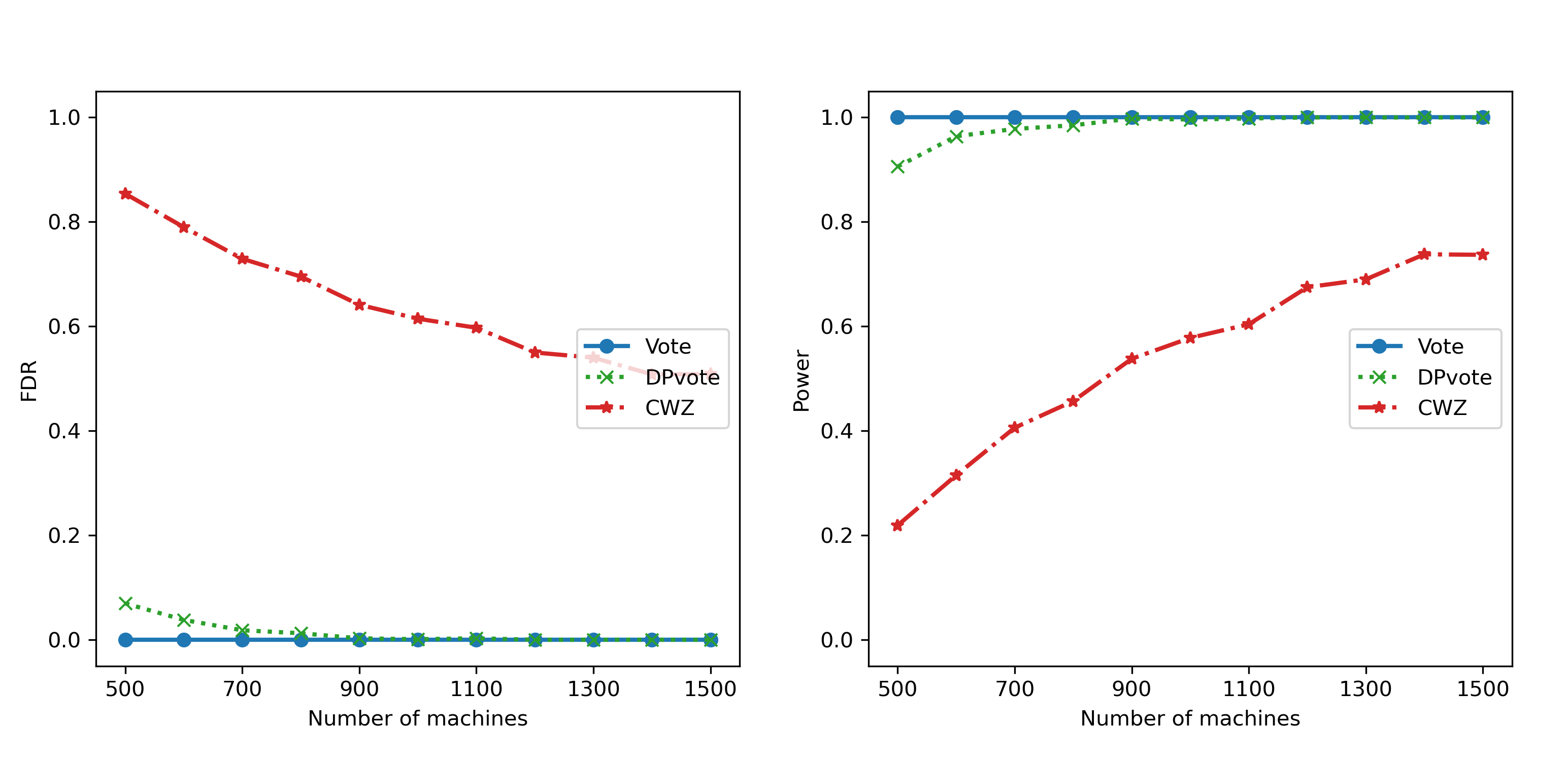
Figure 2: The FDR and Power over the number of machines for sparse mean estimation. The number of machines varies from $500$ to $1500$, the local sample size is $500$, and the dimension $p$ is $500$.

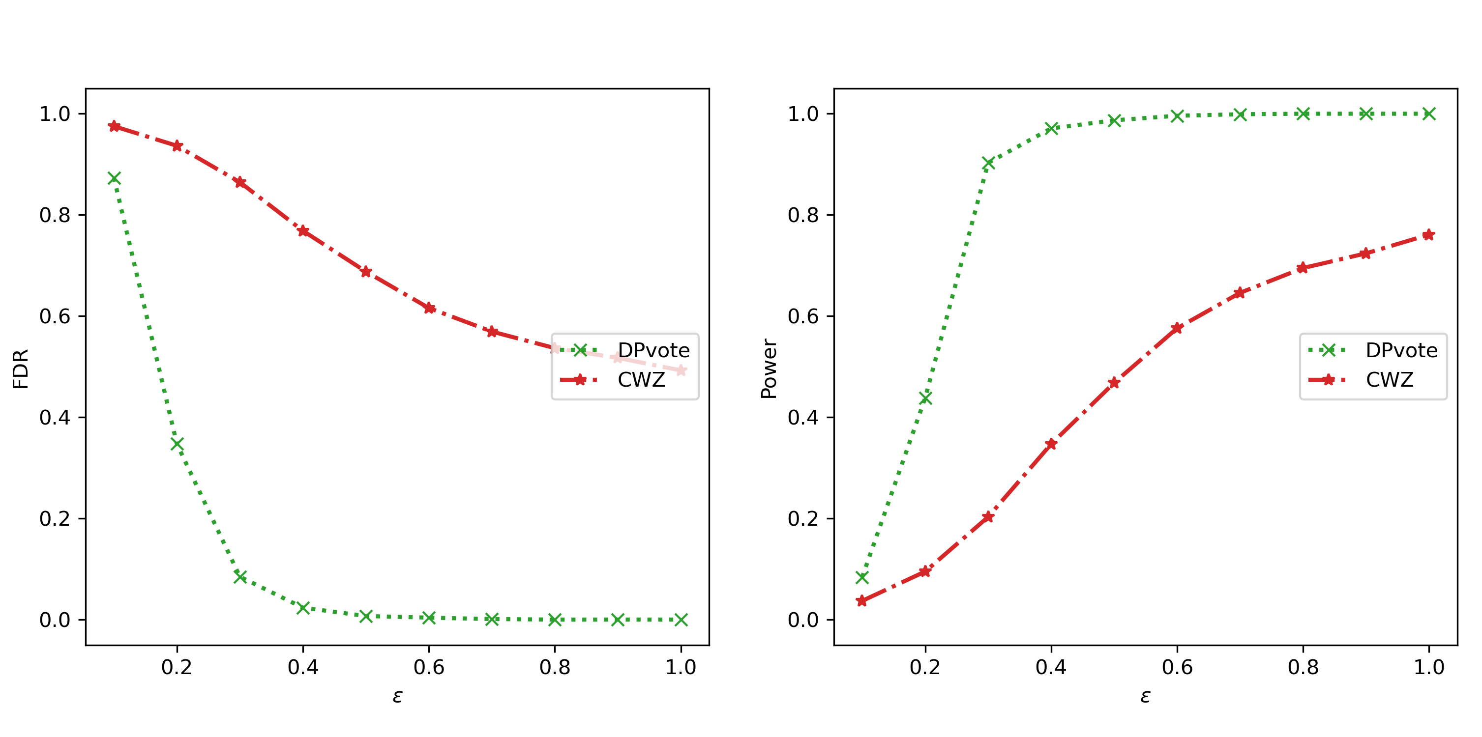
Figure 3: The FDR and Power over the privacy level $\epsilon$ for sparse mean estimation. The local sample size is $500$, the number of machines is $800$, and the dimension $p$ is $500$.

5.2 Results for Sparse Linear Regression

In this section, we consider the linear model defined in (13). The i.i.d. noises $z_{i}$’s are drawn from ${\mathcal{N}}(0,1)$ and the i.i.d. covariate vectors $\boldsymbol{X}_{i}=(X_{i,1},\dots,X_{i,p})^{{\rm T}}$ ($i=1,\dots,N$) are drawn from a multivariate normal distribution ${\mathcal{N}}(\boldsymbol{0},\boldsymbol{\Sigma})$. The covariance matrix $\boldsymbol{\Sigma}$ is a $p\times p$ Toeplitz matrix with its $(i,j)$-th entry $\Sigma_{ij}=0.5^{|i-j|}$, where $1\leq i,j\leq p$. We fix the dimension $p=200$. Moreover, we set the true coefficient $\boldsymbol{\theta}^{*}$ to be the same as $\boldsymbol{\theta}^{*}$ in (21). In the CWZ method proposed in Cai et al. (2021), we take the truncation level $R$ to be $2$, the number of steps $T$ to be 20, and the step size $\eta$ to be $0.1$.

We adopt the same settings as the counterpart in the experiment for sparse mean estimation. The $\mathrm{FDR}$ and $\mathrm{Power}$ are presented in Figures 4 and 5. It is not surprising that all these methods perform similarly to the mean estimation. That is, with the increasing of the number of machines $m$ or the privacy level $\epsilon$, the $\mathrm{FDR}$ of DPVote goes to zero and $\mathrm{Power}$ goes to one. Again, DPVote outperforms $\mathrm{CWZ}$ on all settings.

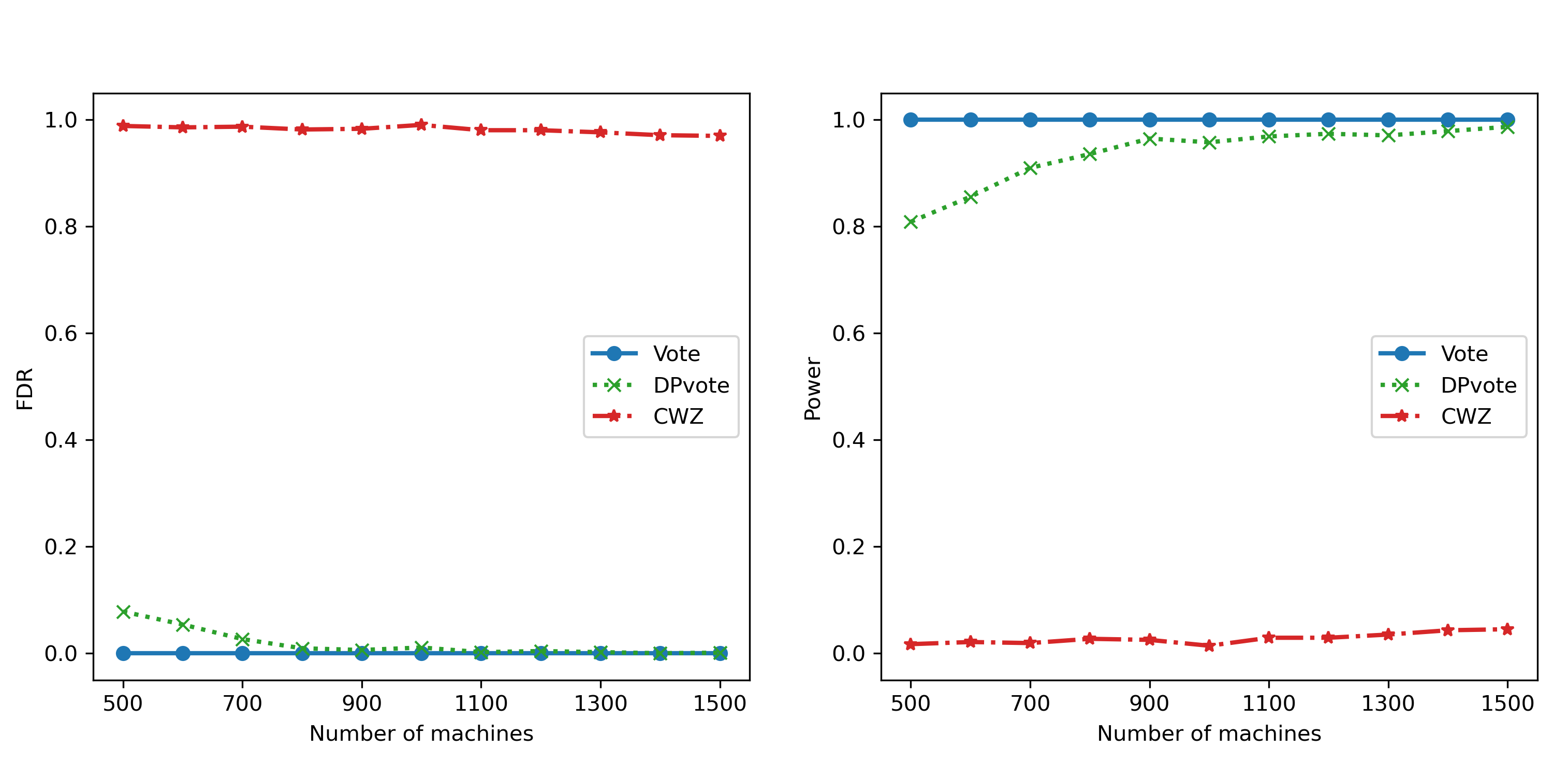
Figure 4: The FDR and Power over the number of machines for sparse linear regression. The number of machines varies from $500$ to $1500$, the local sample size is $500$, and the dimension $p$ is $500$.

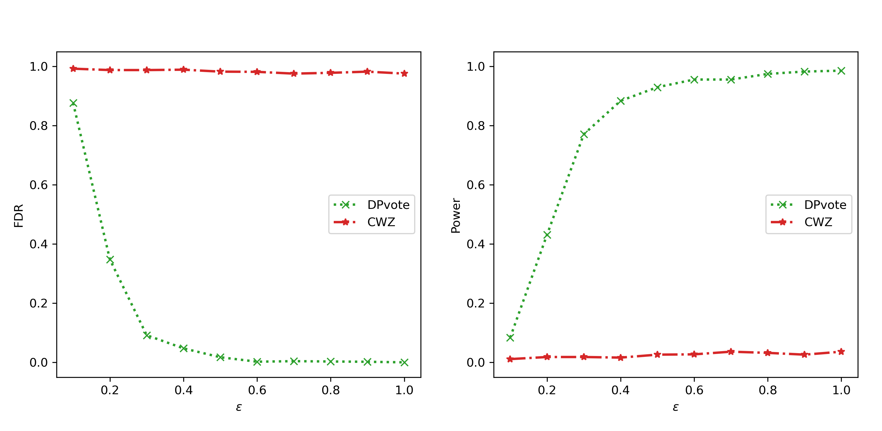
Figure 5: The FDR and Power over the privacy level $\epsilon$ for sparse linear regression. The local sample size is $500$, the number of machines is $800$, and the dimension $p$ is $500$.

6 Conclusion

In summary, this paper considers the sign selection problem under privacy constraints and applies it to the private variable selection for sparse mean vector and sparse linear regression in a distributed setup. With the differentially private majority vote algorithm, we can recover the signs consistently. The admissible signal-to-noise ratio can have the same order as the non-private algorithm. In the future, it would be interesting to study the sparse recovery problems for the matrix-valued problems. Moreover, it is also interesting to consider applying our method to the debias-Lasso problem (Javanmard and Montanari, 2014; Lee et al., 2017; Javanmard and Montanari, 2018).

7 Appendix

7.1 Proof of Results in Section 2.4

Proof of Theorem 1.

Notice that the stability function $f^{S}(\cdot)$ has sensitive $2$. By Lemma 2.4 of Dwork et al. (2021), we know each round of selection is $(\epsilon^{\prime},0)$ private, where

$$\epsilon^{\prime}=\frac{\epsilon}{4\sqrt{2\widetilde{s}\log(2/\delta)}}.$$

Then by advanced composition theorem (Lemma 3), we know the selection of the set $\widetilde{S}$ with $\widetilde{s}$ indices is $(\frac{\epsilon}{2},\frac{\delta}{2})$-differentially private. Notice that the functions $f_{l}(\cdot,1),f_{l}(\cdot,-1),f_{l}(\cdot,0)$ all have global sensitivity $2$. By Theorem 3.10 of Dwork and Roth (2014), for every $l\in\widetilde{S}$, the generation of $\widehat{Q}_{l}$ is $(\epsilon^{\prime},0)$-differentially private. Then by advanced composition theorem (Lemma 3), we know the generation of the $\widetilde{s}$-tuple $\{\widehat{Q}_{l}|l\in\widetilde{S}\}$ is $(\frac{\epsilon}{2},\frac{\delta}{2})$-differentially private. Next, we apply the composition theorem (Lemma 2) and conclude that the composition of these two mechanisms is $(\epsilon,\delta)$-differentially private. ∎

Proof of Theorem 2.

To prove the selection consistency of DPVote, we first prove the consistency of Peeling.

Consistency of Peeling: Let us directly consider the extreme case, where $f^{S}(\boldsymbol{Q}_{l}^{r})=\lceil 8\gamma\sqrt{2\widetilde{s}\log(2/\delta)}\log p\rceil$ for $l\in\,\hbox{\kern 0.09995pt\vbox{\hrule height=0.5pt\kern 1.42082pt\hbox{\kern-1.00006pt$S$\kern-1.00006pt}}}\,$, and $f^{S}(\boldsymbol{Q}_{l}^{r})=0$ for $l\notin\,\hbox{\kern 0.09995pt\vbox{\hrule height=0.5pt\kern 1.42082pt\hbox{\kern-1.00006pt$S$\kern-1.00006pt}}}\,$. Clearly the probability of DPVote algorithm produces the correct signs for any dataset ${\mathbb{Q}}$ is not less than this case. For simplicity denote it as ${\mathbb{P}}(\text{extreme})$.

On the other hand, for the $t$-th selection step (where $1\leq t\leq\widetilde{s}$), suppose there left $\,\hbox{\kern 0.09995pt\vbox{\hrule height=0.5pt\kern 1.42082pt\hbox{\kern-1.00006pt$s$\kern-1.00006pt}}}\,-t+1$ elements in    $S$   and $p-\,\hbox{\kern 0.09995pt\vbox{\hrule height=0.5pt\kern 1.42082pt\hbox{\kern-1.00006pt$s$\kern-1.00006pt}}}\,$ elements in $\,\hbox{\kern 0.09995pt\vbox{\hrule height=0.5pt\kern 1.42082pt\hbox{\kern-1.00006pt$S$\kern-1.00006pt}}}\,^{c}$, the probability that the peeling algorithm select element in    $S$   is greater than the case when there left only one element in    $S$  , let’s denote this probability as ${\mathbb{P}}(1\text{ vs }p-\,\hbox{\kern 0.09995pt\vbox{\hrule height=0.5pt\kern 1.42082pt\hbox{\kern-1.00006pt$s$\kern-1.00006pt}}}\,)$. Since each round of selection is independent, we know

$${\mathbb{P}}(\text{extreme})\geq{\mathbb{P}}^{\,\hbox{\kern 0.06996pt\vbox{\hrule height=0.5pt\kern 0.99458pt\hbox{\kern-0.70004pt$s$\kern-0.70004pt}}}\,}(1\text{ vs }p-\,\hbox{\kern 0.09995pt\vbox{\hrule height=0.5pt\kern 1.42082pt\hbox{\kern-1.00006pt$s$\kern-1.00006pt}}}\,).$$ (22)

Therefore, it left to bound the probability ${\mathbb{P}}(1\text{ vs }p-\,\hbox{\kern 0.09995pt\vbox{\hrule height=0.5pt\kern 1.42082pt\hbox{\kern-1.00006pt$s$\kern-1.00006pt}}}\,)$.

By Lemma 6, we know that

$${\mathbb{P}}(\max_{l\notin\,\hbox{\kern 0.06996pt\vbox{\hrule height=0.5pt\kern 0.99458pt\hbox{\kern-0.70004pt$S$\kern-0.70004pt}}}\,}f^{S}(\boldsymbol{Q}_{l}^{r})+g_{l}\geq 0)\leq{\mathbb{P}}(\max_{l\notin\,\hbox{\kern 0.06996pt\vbox{\hrule height=0.5pt\kern 0.99458pt\hbox{\kern-0.70004pt$S$\kern-0.70004pt}}}\,}g_{l}\geq 8\gamma\sqrt{2\widetilde{s}\log(2/\delta)}\log p)\leq p^{-\gamma+1},$$

$${\mathbb{P}}(\max_{l\in\,\hbox{\kern 0.06996pt\vbox{\hrule height=0.5pt\kern 0.99458pt\hbox{\kern-0.70004pt$S$\kern-0.70004pt}}}\,}f^{S}(\boldsymbol{Q}_{l}^{r})+g_{l}\leq 0)\leq{\mathbb{P}}(\max_{l\in\,\hbox{\kern 0.06996pt\vbox{\hrule height=0.5pt\kern 0.99458pt\hbox{\kern-0.70004pt$S$\kern-0.70004pt}}}\,}g_{l}\leq-8\gamma\sqrt{2\widetilde{s}\log(2/\delta)}\log p)\leq p^{-\gamma+1}.$$

Therefore,

$${\mathbb{P}}(1\text{ vs }p-\,\hbox{\kern 0.09995pt\vbox{\hrule height=0.5pt\kern 1.42082pt\hbox{\kern-1.00006pt$s$\kern-1.00006pt}}}\,)\geq 1-{\mathbb{P}}(\max_{l\notin\,\hbox{\kern 0.06996pt\vbox{\hrule height=0.5pt\kern 0.99458pt\hbox{\kern-0.70004pt$S$\kern-0.70004pt}}}\,}f^{S}(\boldsymbol{Q}_{l}^{r})+g_{l}\geq 0)-{\mathbb{P}}(\max_{l\in\,\hbox{\kern 0.06996pt\vbox{\hrule height=0.5pt\kern 0.99458pt\hbox{\kern-0.70004pt$S$\kern-0.70004pt}}}\,}f^{S}(\boldsymbol{Q}_{l}^{r})+g_{l}\leq 0)\geq 1-2p^{-\gamma+1}.$$

Plugging it into (22) we have that

$${\mathbb{P}}(\text{extreme})\geq{\mathbb{P}}^{\,\hbox{\kern 0.06996pt\vbox{\hrule height=0.5pt\kern 0.99458pt\hbox{\kern-0.70004pt$s$\kern-0.70004pt}}}\,}(1\text{ vs }p-\,\hbox{\kern 0.09995pt\vbox{\hrule height=0.5pt\kern 1.42082pt\hbox{\kern-1.00006pt$s$\kern-1.00006pt}}}\,)\geq(1-2p^{-\gamma+1})^{\,\hbox{\kern 0.06996pt\vbox{\hrule height=0.5pt\kern 0.99458pt\hbox{\kern-0.70004pt$s$\kern-0.70004pt}}}\,}\geq 1-2\,\hbox{\kern 0.09995pt\vbox{\hrule height=0.5pt\kern 1.42082pt\hbox{\kern-1.00006pt$s$\kern-1.00006pt}}}\,p^{-\gamma+1}\geq 1-O(p^{-\gamma+2}),$$ (23)

which proves the first part.

Consistency of DPVote: Suppose the Peeling algorithm has selected the support covering    $S$  , i.e. $\,\hbox{\kern 0.09995pt\vbox{\hrule height=0.5pt\kern 1.42082pt\hbox{\kern-1.00006pt$S$\kern-1.00006pt}}}\,\subseteq\widetilde{S}$. For each $l\in\,\hbox{\kern 0.09995pt\vbox{\hrule height=0.5pt\kern 1.42082pt\hbox{\kern-1.00006pt$S$\kern-1.00006pt}}}\,$, without loss of generality assume $\,\hbox{\kern 0.09995pt\vbox{\hrule height=0.5pt\kern 1.42082pt\hbox{\kern-1.00006pt$Q$\kern-1.00006pt}}}\,_{l}=1$. Then from assumption we know

$$f^{S}(\boldsymbol{Q}_{l}^{r})=N_{l}^{+}-N_{l}^{0}-N_{l}^{-}\geq 8(\gamma+1)\sqrt{2\widetilde{s}\log(2/\delta)}\log p/\epsilon.$$

Then we have that

$${\mathbb{P}}(\widehat{Q}_{l}=1)= \frac{P_{l}^{+}}{P_{l}^{+}+P_{l}^{-}+P_{l}^{0}}$$

$$= \frac{1}{1+\exp\{\epsilon^{\prime}(N^{0}_{l}-N^{+}_{l}+N_{l}^{-})/2\}+\exp\{\epsilon^{\prime}(N^{-}_{l}-N^{+}_{l})/2\}}$$

$$\geq \frac{1}{1+\exp\{-\epsilon^{\prime}f_{l}(\boldsymbol{Q}_{l}^{r},1)/2\}+\exp\{\epsilon^{\prime}f_{l}(\boldsymbol{Q}_{l}^{r},1)/2\}}$$

$$\geq \frac{1}{1+2p^{-\gamma-1}}\geq 1-2p^{-\gamma-1}.$$

For $l\in\widetilde{S}\backslash\,\hbox{\kern 0.09995pt\vbox{\hrule height=0.5pt\kern 1.42082pt\hbox{\kern-1.00006pt$S$\kern-1.00006pt}}}\,$, we have that

$${\mathbb{P}}(\widehat{Q}_{l}=0)= \frac{P_{l}^{0}}{P_{l}^{+}+P_{l}^{-}+P_{l}^{0}}$$

$$= \frac{1}{1+\exp\{-\epsilon^{\prime}\min\{N^{0}_{l}-N^{+}_{l}+N^{-}_{l},N_{l}^{0}\}/2\}+\exp\{\epsilon^{\prime}\min\{N^{0}_{l}-N^{-}_{l}+N^{+}_{l},N_{l}^{0}\}/2\}}$$

$$\geq \frac{1}{1+2\exp\{-\epsilon^{\prime}\min\{N^{0}_{l}-N^{+}_{l}+N^{-}_{l},N^{0}_{l}+N^{+}_{l}-N^{-}_{l}\}/2\}}$$

$$\geq \frac{1}{1+2p^{-\gamma-1}}\geq 1-2p^{-\gamma-1}.$$

Then we have that

$${\mathbb{P}}(\widehat{Q}_{l}=\,\hbox{\kern 0.09995pt\vbox{\hrule height=0.5pt\kern 1.42082pt\hbox{\kern-1.00006pt$Q$\kern-1.00006pt}}}\,_{l},l\in\widetilde{S})=\prod_{l\in\widetilde{S}}{\mathbb{P}}(\widehat{Q}_{l}=\,\hbox{\kern 0.09995pt\vbox{\hrule height=0.5pt\kern 1.42082pt\hbox{\kern-1.00006pt$Q$\kern-1.00006pt}}}\,_{l})\geq(1-2p^{-\gamma-1})^{\,\hbox{\kern 0.06996pt\vbox{\hrule height=0.5pt\kern 0.99458pt\hbox{\kern-0.70004pt$s$\kern-0.70004pt}}}\,}\geq 1-2\,\hbox{\kern 0.09995pt\vbox{\hrule height=0.5pt\kern 1.42082pt\hbox{\kern-1.00006pt$s$\kern-1.00006pt}}}\,p^{-\gamma-1}\geq 1-p^{-\gamma}.$$

Therefore,

$${\mathbb{P}}(\text{{DPVote}}\text{ recovers }\,\hbox{\kern 0.09995pt\vbox{\hrule height=0.5pt\kern 1.42082pt\hbox{\kern-1.00006pt$\boldsymbol{Q}$\kern-1.00006pt}}}\,)\geq{\mathbb{P}}(\widehat{Q}_{l}=\,\hbox{\kern 0.09995pt\vbox{\hrule height=0.5pt\kern 1.42082pt\hbox{\kern-1.00006pt$Q$\kern-1.00006pt}}}\,_{l},l\in\widetilde{S})-(1-{\mathbb{P}}(\text{extreme}))\geq 1-p^{-\gamma}-p^{-\gamma+2}=1-O(p^{-\gamma+2}),$$

which proves the Theorem 2.

∎

Lemma 5.

(Theorem 1 of Arratia et al. (1989)) Let $\{g_{i}|i\in I\}$ be the collection of random variables on an index set $I$. For each $i\in I$, let $I_{i}$ be a subset of $I$ with $i\in I_{i}$. For a given $x\in{\mathbb{R}}$, set $y=\sum_{i\in I}{\mathbb{P}}(g_{i}>x)$. Then

$$\Big{|}{\mathbb{P}}\Big{(}\max_{i\in I}g_{i}\leq x\Big{)}-e^{-y}\Big{|}\leq(1\wedge y^{-1})(T_{1}+T_{2}+T_{3}),$$ (24)

where

$$T_{1}= \sum_{i\in I}\sum_{j\in I_{i}}{\mathbb{P}}(g_{i}>x){\mathbb{P}}(g_{j}>x),$$

$$T_{2}= \sum_{i\in I}\sum_{j\in I_{i},i\neq j}{\mathbb{P}}(g_{i}>x,g_{j}>x),$$

$$T_{3}= \sum_{i\in I}{\mathbb{E}}\big{[}|{\mathbb{P}}(g_{i}>x|\sigma(g_{j},j\notin I_{i}))-{\mathbb{P}}(g_{i}>x)|\big{]}.$$

Lemma 6.

Let $g_{1},\dots,g_{p}$ be $p$ i.i.d. random variable sampled from $\mathrm{Lap}(\lambda)$, then for each $\gamma\geq 2$ we have that

$${\mathbb{P}}\Big{(}\max_{i\in I}g_{i}>\gamma\lambda\log p\Big{)}\leq p^{-\gamma+1}.$$

Proof.

To apply Lemma 5, we let the index $I=\{1,\dots,p\}$, for every $i$, let $I_{i}=\{i\}$. Then by taking $x=\gamma\lambda\log p$, we know that

$$y =\sum_{i\in I}{\mathbb{P}}(g_{i}>x)=\frac{p}{2}e^{-x/\lambda}=\frac{1}{2}p^{-\gamma+1},$$

$$T_{2} =T_{3}=0,$$

$$T_{1} =p\sum_{i\in I}{\mathbb{P}}^{2}(g_{i}>x)=\frac{p}{4}e^{-2x/\lambda}=\frac{1}{4}p^{-2\gamma+1}.$$

By plugging them into (24) we have that

$$\Big{|}{\mathbb{P}}\Big{(}\max_{i\in I}g_{i}\leq\gamma\lambda\log p\Big{)}-e^{-\frac{1}{2}p^{-\gamma+1}}\Big{|}\leq\frac{1}{4}p^{-2\gamma+1},$$

$$\Rightarrow {\mathbb{P}}\Big{(}\max_{i\in I}g_{i}>\gamma\lambda\log p\Big{)}\leq 1-e^{-\frac{1}{2}p^{-\gamma+1}}+\frac{1}{4}p^{-2\gamma+1}\leq p^{-\gamma+1},$$

which proves the lemma. ∎

7.2 Proof of Results in Section 3.2

Lemma 7.

(Berry-Esseen Theorem, Theorem 9.1.3 in Chow and Teicher (2012)) If $\{X_{i},\;i\geq 1\}$ are i.i.d. mean-zero random variables with ${\mathbb{E}}[X_{i}^{2}]=\sigma^{2},{\mathbb{E}}|X_{i}|^{3}<\infty$. Then there exists a constant $C_{\mathrm{B}}>0$ such that

$$\sup_{-\infty<x<\infty}\left|{\mathbb{P}}\left(\sum_{i=1}^{n}X_{i}<\sqrt{n}\sigma x\right)-\Phi(x)\right|\leq\frac{C_{\mathrm{B}}}{\sqrt{n}}.$$

Lemma 8.

(Exponential Inequality, Lemma 1 in Cai and Liu (2011)) Let $X_{1},...,X_{n}$ be i.i.d. random variables with zero mean. Suppose that there exist some $\eta>0$ and $C>0$ such that ${\mathbb{E}}[X_{i}^{2}e^{\eta|X_{i}|}]\leq C$. Then uniformly for $0<x\leq C$ and $n\geq 1$, there is

$${\mathbb{P}}\left\{\frac{1}{n}\sum_{i=1}^{n}X_{i}\geq(\eta+\eta^{-1})x\right\}\leq\exp\left(-\frac{nx^{2}}{C}\right).$$

Lemma 9.

Let $N$($=mn$) i.i.d. random variables $X_{1},...,X_{N}$ evenly distributed in $m$ subsets ${\mathcal{H}}_{1},...,{\mathcal{H}}_{m}$. Suppose ${\mathbb{E}}[X_{i}]=0,{\mathbb{E}}[X_{i}^{2}]=\sigma^{2},{\mathbb{E}}|X_{i}|^{3}<\infty$. Denote $\,\hbox{\kern 0.09995pt\vbox{\hrule height=0.5pt\kern 1.42082pt\hbox{\kern-1.00006pt$X$\kern-1.00006pt}}}\,_{j}=\sum_{i\in{\mathcal{H}}_{j}}X_{i}/n$ as the local sample mean on ${\mathcal{H}}_{j}$. For every $\gamma>1$ and non-negative constant $k$, denote

$$c_{\gamma,k}=\widetilde{C}\left(\frac{1}{n}+\frac{k}{m\sqrt{n}}+\sqrt{\frac{\gamma\log p}{mn}}\right),$$

where $\widetilde{C}>0$ is sufficiently large enough. Then there is

$${\mathbb{P}}\left\{\sum_{j=1}^{m}{\mathbb{I}}\left(\,\hbox{\kern 0.09995pt\vbox{\hrule height=0.5pt\kern 1.42082pt\hbox{\kern-1.00006pt$X$\kern-1.00006pt}}}\,_{j}<c_{\gamma,k}\right)\leq\frac{m}{2}+k\right\}+{\mathbb{P}}\left\{\sum_{j=1}^{m}{\mathbb{I}}\left(\,\hbox{\kern 0.09995pt\vbox{\hrule height=0.5pt\kern 1.42082pt\hbox{\kern-1.00006pt$X$\kern-1.00006pt}}}\,_{j}>-c_{\gamma,k}\right)\leq\frac{m}{2}+k\right\}=O(p^{-\gamma}).$$ (25)

Proof.

For every $x>0$, there is

$${\mathbb{P}}\left\{\sum_{j=1}^{m}{\mathbb{I}}\left(\,\hbox{\kern 0.09995pt\vbox{\hrule height=0.5pt\kern 1.42082pt\hbox{\kern-1.00006pt$X$\kern-1.00006pt}}}\,_{j}<x\right)\leq\frac{m}{2}+k\right\}$$

$$= {\mathbb{P}}\left\{\frac{1}{m}\sum_{j=1}^{m}{\mathbb{I}}\left(\,\hbox{\kern 0.09995pt\vbox{\hrule height=0.5pt\kern 1.42082pt\hbox{\kern-1.00006pt$X$\kern-1.00006pt}}}\,_{j}<x\right)-{\mathbb{P}}\left(\,\hbox{\kern 0.09995pt\vbox{\hrule height=0.5pt\kern 1.42082pt\hbox{\kern-1.00006pt$X$\kern-1.00006pt}}}\,_{1}<x\right)\leq\frac{1}{2}+\frac{k}{m}-{\mathbb{P}}\left(\,\hbox{\kern 0.09995pt\vbox{\hrule height=0.5pt\kern 1.42082pt\hbox{\kern-1.00006pt$X$\kern-1.00006pt}}}\,_{1}<x\right)\right\}$$

$$\leq {\mathbb{P}}\left\{\frac{1}{m}\sum_{j=1}^{m}{\mathbb{I}}\left(\,\hbox{\kern 0.09995pt\vbox{\hrule height=0.5pt\kern 1.42082pt\hbox{\kern-1.00006pt$X$\kern-1.00006pt}}}\,_{j}<x\right)-{\mathbb{P}}\left(\,\hbox{\kern 0.09995pt\vbox{\hrule height=0.5pt\kern 1.42082pt\hbox{\kern-1.00006pt$X$\kern-1.00006pt}}}\,_{1}<x\right)\leq\frac{1}{2}+\frac{k}{m}+\frac{C_{\mathrm{B}}}{\sqrt{n}}-\Phi\left(\frac{\sqrt{n}x}{\sigma}\right)\right\}$$

$$= {\mathbb{P}}\left\{\frac{1}{m}\sum_{j=1}^{m}{\mathbb{I}}\left(\,\hbox{\kern 0.09995pt\vbox{\hrule height=0.5pt\kern 1.42082pt\hbox{\kern-1.00006pt$X$\kern-1.00006pt}}}\,_{j}<x\right)-{\mathbb{P}}\left(\,\hbox{\kern 0.09995pt\vbox{\hrule height=0.5pt\kern 1.42082pt\hbox{\kern-1.00006pt$X$\kern-1.00006pt}}}\,_{1}<x\right)\leq-\sqrt{\frac{C\gamma\log p}{m}}\right\},$$

where the last line uses Berry-Esseen Theorem (Lemma 7), and $x$ is given by

$$x=\frac{\sigma}{\sqrt{n}}\Phi^{-1}\left(\frac{1}{2}+\frac{k}{m}+\frac{C_{\mathrm{B}}}{\sqrt{n}}+\sqrt{\frac{C\gamma\log p}{m}}\right).$$

Applying Lemma 8 to the i.i.d. sequence ${\mathbb{I}}\left(\,\hbox{\kern 0.09995pt\vbox{\hrule height=0.5pt\kern 1.42082pt\hbox{\kern-1.00006pt$X$\kern-1.00006pt}}}\,_{j}<x\right)-{\mathbb{P}}\left(\,\hbox{\kern 0.09995pt\vbox{\hrule height=0.5pt\kern 1.42082pt\hbox{\kern-1.00006pt$X$\kern-1.00006pt}}}\,_{1}<x\right)$, we have

$${\mathbb{P}}\left\{\frac{1}{m}\sum_{j=1}^{m}{\mathbb{I}}\left(\,\hbox{\kern 0.09995pt\vbox{\hrule height=0.5pt\kern 1.42082pt\hbox{\kern-1.00006pt$X$\kern-1.00006pt}}}\,_{j}<x\right)-{\mathbb{P}}\left(\,\hbox{\kern 0.09995pt\vbox{\hrule height=0.5pt\kern 1.42082pt\hbox{\kern-1.00006pt$X$\kern-1.00006pt}}}\,_{1}<x\right)\leq-\sqrt{\frac{C\gamma\log p}{m}}\right\}=O(p^{-\gamma}),$$

for some $C$ large enough. Moreover, we have the following elementary facts

$$\big{|}\Phi^{-1}(x_{0})\big{|}=\big{|}\Phi^{-1}(x_{0})-\Phi^{-1}\left(1/2\right)\big{|}\leq\left|x_{0}-1/2\right|\left(\Phi^{-1}\right)^{\prime}(x_{0})\leq\frac{|x_{0}-1/2|}{\psi\left\{\Phi^{-1}(3/4)\right\}},$$

holds for any $1/4\leq x_{0}<3/4$. On the other hand, we know that $1/4\leq\Phi(\sqrt{n}x/\sigma)<3/4$ holds for $m,n$ sufficiently large. Denote $C_{\delta}=1/\psi\{\Phi^{-1}(3/4)\}$, then there is

$${\mathbb{P}}\left\{\sum_{j=1}^{m}{\mathbb{I}}\left(\,\hbox{\kern 0.09995pt\vbox{\hrule height=0.5pt\kern 1.42082pt\hbox{\kern-1.00006pt$X$\kern-1.00006pt}}}\,_{j}<\frac{C_{\delta}\sigma}{\sqrt{n}}\left(\frac{C_{\mathrm{B}}}{\sqrt{n}}+\frac{k}{m}+\sqrt{\frac{C\gamma\log p}{m}}\right)\right)\leq\frac{m}{2}\right\}$$

$$\leq {\mathbb{P}}\left\{\frac{1}{m}\sum_{j=1}^{m}{\mathbb{I}}\left(\,\hbox{\kern 0.09995pt\vbox{\hrule height=0.5pt\kern 1.42082pt\hbox{\kern-1.00006pt$X$\kern-1.00006pt}}}\,_{j}<x\right)-{\mathbb{P}}\left(\,\hbox{\kern 0.09995pt\vbox{\hrule height=0.5pt\kern 1.42082pt\hbox{\kern-1.00006pt$X$\kern-1.00006pt}}}\,_{1}<x\right)\leq-\sqrt{\frac{C\gamma\log p}{m}}\right\}\leq p^{-\gamma}.$$

Therefore, if we choose $\widetilde{C}\geq\max\{C_{\delta}C_{B}\sigma,C_{\delta}\sqrt{C}\sigma\}$, the bound of the first term in the left hand side of (25) is proved. By repeating the same procedure, we can prove the bound of the second term, which yields the desired result. ∎

Before proving Theorem 3, we shall first prove the following proposition.

Proposition 1.

(Sign consistency of MajVote) Let $N=mn$ i.i.d. random vectors $\{\boldsymbol{X}_{1},\dots,\boldsymbol{X}_{N}\}$ be sampled from ${\mathcal{P}}(\boldsymbol{\theta}^{*},C)$. Moreover, there are sufficiently large constants $C_{3},C_{4},\gamma_{0}>0$, such that

• The dimension $p$ satisfies $p=O(n^{\gamma_{0}})$, and take $\lambda_{N}=C_{3}(\sqrt{\log p/N}+1/n)$;

• Denote $S=\mathrm{supp}(\boldsymbol{\theta}^{*})$, then there is $\min_{l\in S}|\theta_{l}^{*}|\geq C_{4}\lambda_{N}$.

Then $\,\hbox{\kern 0.09995pt\vbox{\hrule height=0.5pt\kern 1.42082pt\hbox{\kern-1.00006pt$\boldsymbol{Q}$\kern-1.00006pt}}}\,({\mathbb{X}})$ defined in (9) satisfies that, for some large $\gamma_{2}$ depends on $C_{1},C_{2},\gamma_{0}$, there is

$${\mathbb{P}}\Big{(}\,\hbox{\kern 0.09995pt\vbox{\hrule height=0.5pt\kern 1.42082pt\hbox{\kern-1.00006pt$\boldsymbol{Q}$\kern-1.00006pt}}}\,({\mathbb{X}})={\rm sgn}(\boldsymbol{\theta}^{*})\Big{)}\geq 1-O(p^{-\gamma_{2}}).$$

Proof of Proposition 1.

If we can show that

$$\max_{1\leq l\leq p}{\mathbb{P}}\Big{(}\,\hbox{\kern 0.09995pt\vbox{\hrule height=0.5pt\kern 1.42082pt\hbox{\kern-1.00006pt$Q$\kern-1.00006pt}}}\,_{l}({\mathbb{X}})\neq{\rm sgn}(\theta_{l}^{*})\Big{)}=O(p^{-\gamma}),$$ (26)

where $\gamma>0$ is large enough. Then this theorem is proved as follows

$$1-{\mathbb{P}}\Big{(}\,\hbox{\kern 0.09995pt\vbox{\hrule height=0.5pt\kern 1.42082pt\hbox{\kern-1.00006pt$\boldsymbol{Q}$\kern-1.00006pt}}}\,({\mathbb{X}})={\rm sgn}(\boldsymbol{\theta}^{*})\Big{)}$$

$$\leq p\max_{1\leq l\leq p}{\mathbb{P}}\Big{(}\,\hbox{\kern 0.09995pt\vbox{\hrule height=0.5pt\kern 1.42082pt\hbox{\kern-1.00006pt$Q$\kern-1.00006pt}}}\,_{l}({\mathbb{X}})\neq{\rm sgn}(\theta_{l}^{*})\Big{)}=O(pp^{-\gamma})=O(p^{-\gamma+\gamma_{0}}),$$

provided that $\gamma>\gamma_{0}$ and sufficient large $\gamma_{0}$. For the $l$-th coordinate, we firstly suppose that $\theta_{l}^{*}=0$. Since $\boldsymbol{X}_{i}$’s are sampled from the distribution (10), by Lemma 9 with $k=0$, if

$$\lambda_{N}=C_{0}\left(\sqrt{\frac{\log p}{mn}}+\frac{1}{n}\right)\geq c_{\gamma,0},$$

we have

$${\mathbb{P}}\Big{(}\,\hbox{\kern 0.09995pt\vbox{\hrule height=0.5pt\kern 1.42082pt\hbox{\kern-1.00006pt$Q$\kern-1.00006pt}}}\,_{l}({\mathbb{X}})\neq{\rm sgn}(\theta_{l}^{*})\Big{)}$$

$$\leq {\mathbb{P}}\Big{\{}\sum_{j=1}^{m}{\mathbb{I}}\Big{(}\,\hbox{\kern 0.09995pt\vbox{\hrule height=0.5pt\kern 1.42082pt\hbox{\kern-1.00006pt$X$\kern-1.00006pt}}}\,_{j,l}<\lambda_{N}\Big{)}\leq\frac{m}{2}\Big{\}}+{\mathbb{P}}\Big{\{}\sum_{j=1}^{m}{\mathbb{I}}\Big{(}\,\hbox{\kern 0.09995pt\vbox{\hrule height=0.5pt\kern 1.42082pt\hbox{\kern-1.00006pt$X$\kern-1.00006pt}}}\,_{j,l}>-\lambda_{N}\Big{)}\leq\frac{m}{2}\Big{\}}=O(p^{-\gamma}).$$

Next we assume $\theta_{l}^{*}>0$. We use Lemma 9 again, if

$$\theta_{l}^{*}\geq C_{1}\Big{(}\sqrt{\frac{\log p}{mn}}+\frac{1}{n}\Big{)}\geq c_{\gamma,0}+\lambda_{N},$$

then there is

$${\mathbb{P}}\Big{(}\,\hbox{\kern 0.09995pt\vbox{\hrule height=0.5pt\kern 1.42082pt\hbox{\kern-1.00006pt$Q$\kern-1.00006pt}}}\,_{l}({\mathbb{X}})\neq{\rm sgn}(\theta_{l}^{*})\Big{)}\leq{\mathbb{P}}\Big{\{}\sum_{j=1}^{m}{\mathbb{I}}\Big{(}\,\hbox{\kern 0.09995pt\vbox{\hrule height=0.5pt\kern 1.42082pt\hbox{\kern-1.00006pt$X$\kern-1.00006pt}}}\,_{j,l}>\lambda_{N}\Big{)}\leq\frac{m}{2}\Big{\}}$$

$$\leq {\mathbb{P}}\Big{\{}\sum_{j=1}^{m}{\mathbb{I}}\Big{(}\,\hbox{\kern 0.09995pt\vbox{\hrule height=0.5pt\kern 1.42082pt\hbox{\kern-1.00006pt$X$\kern-1.00006pt}}}\,_{j,l}-\theta_{l}^{*}>-c_{\gamma,0}\Big{)}\leq\frac{m}{2}\Big{\}}=O(p^{-\gamma}).$$

Lastly, when $\theta_{l}^{*}<0$, the proof is the same as above. Therefore (26) is proved. ∎

Proof of Theorem 3.

By Theorem 1, we know that $\,\hbox{\kern 0.09995pt\vbox{\hrule height=0.5pt\kern 1.42082pt\hbox{\kern-1.00006pt$\boldsymbol{Q}$\kern-1.00006pt}}}\,({\mathbb{X}})={\rm sgn}(\boldsymbol{\theta}^{*})$ holds with probability not less than $1-p^{-\gamma_{1}}$. To prove the sign consistency of $\widehat{\boldsymbol{Q}}({\mathbb{X}})$, from Theorem 2 we know that it is enough to show for each $l\in S$, there is

$$f^{S}(\boldsymbol{Q}^{r}_{l})\geq 8(\gamma+1)\sqrt{2\widetilde{s}\log(2/\delta)}\log p/\epsilon$$

hold with probability $1-O(p^{-\gamma})$. For $l\in S$, without loss of generality assume that ${\rm sgn}(\theta^{*}_{l})={\rm sgn}(\,\hbox{\kern 0.09995pt\vbox{\hrule height=0.5pt\kern 1.42082pt\hbox{\kern-1.00006pt$Q$\kern-1.00006pt}}}\,_{l}({\mathbb{X}}))=1$, then

$$f_{l}(\boldsymbol{Q}^{r}_{l},\,\hbox{\kern 0.09995pt\vbox{\hrule height=0.5pt\kern 1.42082pt\hbox{\kern-1.00006pt$Q$\kern-1.00006pt}}}\,_{l}({\mathbb{X}}))= N_{l}^{+}-N_{l}^{-}-N_{l}^{0}=2N_{l}^{+}-m$$

$$= 2\sum_{j=1}^{m}{\mathbb{I}}\Big{(}\,\hbox{\kern 0.09995pt\vbox{\hrule height=0.5pt\kern 1.42082pt\hbox{\kern-1.00006pt$X$\kern-1.00006pt}}}\,_{j,l}>\lambda_{N}\Big{)}-m$$

$$= 2\Big{\{}\sum_{j=1}^{m}{\mathbb{I}}\Big{(}\,\hbox{\kern 0.09995pt\vbox{\hrule height=0.5pt\kern 1.42082pt\hbox{\kern-1.00006pt$X$\kern-1.00006pt}}}\,_{j,l}-\theta_{l}^{*}>\lambda_{N}-\theta_{l}^{*}\Big{)}-\frac{m}{2}\Big{\}}.$$

Therefore,

$${\mathbb{P}}\Big{(}f^{S}(\boldsymbol{Q}_{l}^{r})\geq 8(\gamma+1)\sqrt{2\widetilde{s}\log(2/\delta)}\log p/\epsilon\Big{)}$$

$$= {\mathbb{P}}\left(\sum_{j=1}^{m}{\mathbb{I}}\Big{(}\,\hbox{\kern 0.09995pt\vbox{\hrule height=0.5pt\kern 1.42082pt\hbox{\kern-1.00006pt$X$\kern-1.00006pt}}}\,_{j,l}-\theta_{l}^{*}>\lambda_{N}-\theta_{l}^{*}\Big{)}-\frac{m}{2}\geq 4(\gamma+1)\sqrt{2\widetilde{s}\log(2/\delta)}\log p/\epsilon\right)$$

$$\geq 1-O(p^{-\gamma_{1}}),$$

as long as

$$\theta_{l}^{*}-\lambda_{N}\geq\frac{C_{\delta}\sigma}{\sqrt{n}}\left(\frac{C_{\mathrm{B}}}{\sqrt{n}}+\frac{4(\gamma+1)\sqrt{2\widetilde{s}\log(2/\delta)}\log p}{m\epsilon}+\sqrt{\frac{C\gamma_{1}\log p}{m}}\right),$$

which proves the first part of the proposition. Similarly, when $\widetilde{s}>s$,for $l\notin S$, there is

$$f_{l}(\boldsymbol{Q}^{r}_{l},0)= \min\{N_{l}^{0}-N_{l}^{+}+N_{l}^{-},N_{l}^{0}+N_{l}^{+}-N_{l}^{-}\}$$

$$= \min\Big{\{}2\sum_{j=1}^{m}{\mathbb{I}}\Big{(}\,\hbox{\kern 0.09995pt\vbox{\hrule height=0.5pt\kern 1.42082pt\hbox{\kern-1.00006pt$X$\kern-1.00006pt}}}\,_{j,l}\leq\lambda_{N}\Big{)},2\sum_{j=1}^{m}{\mathbb{I}}\Big{(}\,\hbox{\kern 0.09995pt\vbox{\hrule height=0.5pt\kern 1.42082pt\hbox{\kern-1.00006pt$X$\kern-1.00006pt}}}\,_{j,l}\geq-\lambda_{N}\Big{)}\Big{\}}-m.$$

Therefore

$${\mathbb{P}}\Big{(}2\sum_{j=1}^{m}{\mathbb{I}}\Big{(}\,\hbox{\kern 0.09995pt\vbox{\hrule height=0.5pt\kern 1.42082pt\hbox{\kern-1.00006pt$X$\kern-1.00006pt}}}\,_{j,l}\leq\lambda_{N}\Big{)}-m\geq 8(\gamma+1)\sqrt{2\widetilde{s}\log(2/\delta)}\log p/\epsilon\Big{)}$$

$$= {\mathbb{P}}\left(\sum_{j=1}^{m}{\mathbb{I}}\Big{(}\,\hbox{\kern 0.09995pt\vbox{\hrule height=0.5pt\kern 1.42082pt\hbox{\kern-1.00006pt$X$\kern-1.00006pt}}}\,_{j,l}\leq\lambda_{N}\Big{)}-\frac{m}{2}\geq 4(\gamma+1)\sqrt{2\widetilde{s}\log(2/\delta)}\log p/\epsilon\right)$$

$$\geq 1-O(p^{-\gamma_{1}}),$$

as long as

$$\lambda_{N}\geq\frac{C_{\delta}\sigma}{\sqrt{n}}\left(\frac{C_{\mathrm{B}}}{\sqrt{n}}+\frac{4(\gamma+1)\sqrt{2\widetilde{s}\log(2/\delta)}\log p}{m\epsilon}+\sqrt{\frac{C\gamma_{1}\log p}{m}}\right).$$

Similarly we can show that

$${\mathbb{P}}\Big{(}2\sum_{j=1}^{m}{\mathbb{I}}\Big{(}\,\hbox{\kern 0.09995pt\vbox{\hrule height=0.5pt\kern 1.42082pt\hbox{\kern-1.00006pt$X$\kern-1.00006pt}}}\,_{j,l}\geq-\lambda_{N}\Big{)}-m\geq 8(\gamma+1)\sqrt{2\widetilde{s}\log(2/\delta)}\log p/\epsilon\Big{)}\geq 1-O(p^{-\gamma_{1}}).$$

Therefore we have

$${\mathbb{P}}\Big{(}f_{l}(\boldsymbol{Q}^{r}_{l},0)\geq 8(\gamma+1)\sqrt{2\widetilde{s}\log(2/\delta)}\log p/\epsilon\Big{)}\geq 1-O(p^{-\gamma_{1}}),$$

and Theorem 2 applies. ∎

7.3 Proof of Results in Section 4.2

Lemma 10.

Let $\boldsymbol{X}_{1},\dots,\boldsymbol{X}_{n}$ be i.i.d. random vectors sampled from the distribution in (17). Denote its covariance matrix as $\boldsymbol{\Sigma}$, and the sample covariance matrix as $\widehat{\boldsymbol{\Sigma}}$. Then for every $\gamma>1$, there exists a constant $\widetilde{C}>0$ such that

$${\mathbb{P}}\Big{(}\left\|\boldsymbol{\Sigma}^{-1}\widehat{\boldsymbol{\Sigma}}-\boldsymbol{I}\right\|_{\infty}\geq\widetilde{C}\sqrt{\frac{\log p}{n}}\Big{)}=O(p^{-\gamma}).$$

Proof.

Recall that the inverse covariance matrix is denoted as $\boldsymbol{\Sigma}^{-1}=(\boldsymbol{\omega}_{1},\dots,\boldsymbol{\omega}_{p})$, and $\boldsymbol{e}_{l}$ as the $l$-th coordinate vector. Then the $(l_{1},l_{2})$-entry of the matrix $\boldsymbol{\Sigma}^{-1}\widehat{\boldsymbol{\Sigma}}-\boldsymbol{I}$ is

$$(\boldsymbol{\Sigma}^{-1}\widehat{\boldsymbol{\Sigma}}-\boldsymbol{I})_{l_{1},l_{2}}=\frac{1}{n}\sum_{i=1}^{n}\boldsymbol{\omega}_{l_{1}}^{{\rm T}}\boldsymbol{X}_{i}\cdot\boldsymbol{e}_{l_{2}}^{{\rm T}}\boldsymbol{X}_{i}-\delta_{l_{1},l_{2}}.$$

Since the dimension $p$ is assumed to be bounded, and the covariance matrix is positive definite, there exist a constant $\rho\in(0,1)$ such that

$$\rho\leq\Lambda_{\min}(\boldsymbol{\Sigma})\leq\Lambda_{\max}(\boldsymbol{\Sigma})\leq\rho^{-1}.$$

Then we have

$$\max_{1\leq l\leq p}|\boldsymbol{\omega}_{l}|_{2}\leq\left\|\boldsymbol{\Sigma}^{-1}\right\|\leq\rho^{-1}.$$

Since $\boldsymbol{X}$ is sub-Gaussian in (17), we obtain

$$\max_{1\leq l_{1},l_{2}\leq p}{\mathbb{E}}\big{\{}\exp\eta_{1}\rho\big{|}\boldsymbol{\omega}_{l_{1}}^{{\rm T}}\boldsymbol{X}_{i}\cdot\boldsymbol{e}_{l_{2}}^{{\rm T}}\boldsymbol{X}_{i}-\delta_{l_{1},l_{2}}\big{|}\big{\}}$$

$$\leq e^{\eta_{1}\rho}\cdot\sup_{|\boldsymbol{v}|_{2}\leq 1}{\mathbb{E}}\big{\{}\eta_{1}|\boldsymbol{v}^{{\rm T}}\boldsymbol{X}|^{2}\big{\}}\leq e^{\eta_{1}\rho}C_{1}.$$

Therefore, we can apply Lemma 8 to each coordinate and yield

$${\mathbb{P}}\Big{(}\left\|\boldsymbol{\Sigma}^{-1}\widehat{\boldsymbol{\Sigma}}-\boldsymbol{I}\right\|_{\infty}\geq\widetilde{C}\sqrt{\frac{\log p}{n}}\Big{)}$$

$$\leq p^{2}\max_{1\leq l_{1},l_{2}\leq p}{\mathbb{P}}\Big{(}\Big{|}\frac{1}{n}\sum_{i=1}^{n}\boldsymbol{\omega}_{l_{1}}^{{\rm T}}\boldsymbol{X}_{i}\cdot\boldsymbol{e}_{l_{2}}^{{\rm T}}\boldsymbol{X}_{i}-\delta_{l_{1},l_{2}}\Big{|}\geq\widetilde{C}\sqrt{\frac{\log p}{n}}\Big{)}$$

$$= O(p^{2}p^{-\gamma-2})=O(p^{-\gamma}),$$

for some $\widetilde{C}$ sufficiently large. Therefore, the lemma is proved. ∎

Before proving Theorem 4, we first provide the sign consistency of the non-private MajVote Lasso estimator. Namely, we define

$$\,\hbox{\kern 0.09995pt\vbox{\hrule height=0.5pt\kern 1.42082pt\hbox{\kern-1.00006pt$\boldsymbol{Q}$\kern-1.00006pt}}}\,({\mathbb{X}})=\text{{MajVote}}({\mathcal{Q}}_{0}(\widehat{\boldsymbol{\theta}}_{j})|1\leq j\leq m).$$ (27)

Then we have the following proposition.

Proposition 2.

(Sign consistency of MajVote Lasso) Let $N=mn$ i.i.d. random vectors ${\mathbb{X}}=\{(\boldsymbol{X}_{1},Y_{1}),\dots,(\boldsymbol{X}_{N},Y_{N})\}$ be sampled from ${\mathcal{P}}_{\boldsymbol{X},Y}(\boldsymbol{\theta}^{*},\rho,\eta_{1},C_{1},\eta_{2},C_{2})$. Moreover, we assume the same conditions as in Theorem 4 holds. Then $\,\hbox{\kern 0.09995pt\vbox{\hrule height=0.5pt\kern 1.42082pt\hbox{\kern-1.00006pt$\boldsymbol{Q}$\kern-1.00006pt}}}\,({\mathbb{X}})$ defined in (27) satisfies that, there is constant $\gamma_{2}>0$ such that

$${\mathbb{P}}\Big{(}\,\hbox{\kern 0.09995pt\vbox{\hrule height=0.5pt\kern 1.42082pt\hbox{\kern-1.00006pt$\boldsymbol{Q}$\kern-1.00006pt}}}\,({\mathbb{X}})={\rm sgn}(\boldsymbol{\theta}^{*})\Big{)}\geq 1-O(p^{-\gamma_{2}}).$$

Proof of Proposition 2.

For each $j\in\{1,\dots,m\}$, taking sub-gradient of (14) at $\widehat{\boldsymbol{\theta}}_{j}$, we have that

$$-\frac{1}{n}\sum_{i\in{\mathcal{H}}_{j}}(Y_{i}-\boldsymbol{X}_{i}^{{\rm T}}\widehat{\boldsymbol{\theta}}_{j})\boldsymbol{X}_{i}+\lambda_{j}\boldsymbol{Z}_{j}=0,$$

where $\boldsymbol{Z}_{j}$ is the sub-gradient satisfying $|\boldsymbol{Z}_{j}|_{\infty}\leq 1$. Rearranging the terms and multiplying $\boldsymbol{\Sigma}^{-1}$ on the both sides, we have

$$\widehat{\boldsymbol{\theta}}_{j}-\boldsymbol{\theta}^{*}=(\boldsymbol{I}-\boldsymbol{\Sigma}^{-1}\frac{1}{n}\sum_{i\in{\mathcal{H}}_{j}}\boldsymbol{X}_{i}\boldsymbol{X}_{i}^{{\rm T}})(\widehat{\boldsymbol{\theta}}_{j}-\boldsymbol{\theta}^{*})+\frac{1}{n}\sum_{i\in{\mathcal{H}}_{j}}\boldsymbol{\Sigma}^{-1}\boldsymbol{X}_{i}z_{i}-\lambda_{j}\boldsymbol{\Sigma}^{-1}\boldsymbol{Z}_{j}.$$ (28)

Taking $\widetilde{\eta}=\min\{\eta_{1}\rho,\eta_{2}\}$, since the noise and covariates are assumed to be sub-Gaussian in (17), for each coordinate $l\in\{1,\dots,p\}$, we have

$$\max_{1\leq l\leq p}{\mathbb{E}}\big{\{}\exp\widetilde{\eta}|\boldsymbol{\omega}_{l}\boldsymbol{X}\cdot z|\big{\}}$$

$$\leq \max_{1\leq l\leq p}{\mathbb{E}}\Big{\{}\exp\Big{(}\frac{1}{2}\eta\rho|\boldsymbol{\omega}_{l}\boldsymbol{X}|^{2}+\frac{1}{2}\eta_{2}|z|^{2}\Big{)}\Big{\}}$$

$$\leq \max_{1\leq l\leq p}\Big{[}{\mathbb{E}}\big{\{}\exp\eta\rho|\boldsymbol{\omega}_{l}\boldsymbol{X}|^{2}\big{\}}\cdot{\mathbb{E}}\big{\{}\exp\eta_{2}|z|^{2}\big{\}}\Big{]}^{1/2}\leq\sqrt{C_{1}C_{2}}.$$

Therefore by Lemma 8, we know that there exists a constant $\widetilde{C}_{1}>0$ such that

$$\max_{1\leq j\leq m}\Big{|}\frac{1}{n}\sum_{i\in{\mathcal{H}}_{j}}\boldsymbol{\Sigma}^{-1}\boldsymbol{X}_{i}z_{i}\Big{|}_{\infty}\leq\widetilde{C}_{1}\sqrt{\frac{\log p}{n}},$$ (29)

with probability larger than $1-O(p^{-\gamma})$. On the other hand, by the fact that $|\boldsymbol{Z}_{j}|_{\infty}\leq 1$, we have

$$|\lambda_{j}\boldsymbol{\Sigma}^{-1}\boldsymbol{Z}_{j}|_{\infty}\leq\lambda_{j}\left\|\boldsymbol{\Sigma}^{-1}\right\|_{L_{\infty}}.$$ (30)

Moreover, since $|\widehat{\boldsymbol{\theta}}_{j}|_{0}\leq\widetilde{s}$ by Lemma 10, we know

$$\max_{1\leq j\leq m}\Big{|}\Big{(}\boldsymbol{I}-\boldsymbol{\Sigma}^{-1}\frac{1}{n}\sum_{i\in{\mathcal{H}}_{j}}\boldsymbol{X}_{i}\boldsymbol{X}_{i}^{{\rm T}}\Big{)}(\widehat{\boldsymbol{\theta}}_{j}-\boldsymbol{\theta}^{*})\Big{|}_{\infty}=O_{{\mathbb{P}}}\Big{(}\widetilde{s}\sqrt{\frac{\log p}{n}}|\widehat{\boldsymbol{\theta}}_{j}-\boldsymbol{\theta}^{*}|_{\infty}\Big{)}\leq\frac{1}{2}|\widehat{\boldsymbol{\theta}}_{j}-\boldsymbol{\theta}^{*}|_{\infty}.$$ (31)

By substituting equations (29), (30), and (31) into (28), we have

$$|\widehat{\boldsymbol{\theta}}_{j}-\boldsymbol{\theta}^{*}|_{\infty}\leq 2\lambda_{j}\left\|\boldsymbol{\Sigma}^{-1}\right\|_{L_{\infty}}+2\widetilde{C}_{1}\sqrt{\frac{\log p}{n}}.$$

From (28), the $l$-th coordinate can be written in the following form

$$\widehat{\theta}_{j,l}-\theta^{*}_{l}=-\lambda_{j}\omega_{l,l}Z_{j,l}-\lambda_{j}\boldsymbol{\omega}^{{\rm T}}_{l,-l}\boldsymbol{Z}_{j,-l}+\frac{1}{n}\sum_{i\in{\mathcal{H}}_{j}}\boldsymbol{\omega}_{l}^{{\rm T}}\boldsymbol{X}_{i}z_{i}+o_{{\mathbb{P}}}\Big{(}\frac{\log p}{n}\Big{)}.$$ (32)

It left to rehash the argument in the proof of Theorem 1. From Lemma 11 below we have that

$$1-{\mathbb{P}}\Big{(}\,\hbox{\kern 0.09995pt\vbox{\hrule height=0.5pt\kern 1.42082pt\hbox{\kern-1.00006pt$\boldsymbol{Q}$\kern-1.00006pt}}}\,({\mathbb{X}})={\rm sgn}(\boldsymbol{\theta}^{*})\Big{)}\leq p\cdot\max_{1\leq l\leq p}{\mathbb{P}}\Big{(}\,\hbox{\kern 0.09995pt\vbox{\hrule height=0.5pt\kern 1.42082pt\hbox{\kern-1.00006pt$Q$\kern-1.00006pt}}}\,_{l}({\mathbb{X}})\neq{\rm sgn}(\theta_{l}^{*})\Big{)}=O(p^{-\gamma+1}).$$

Therefore we proved Proposition 2. ∎

Lemma 11.

Assume the same conditions in Proposition 2. For every $1\leq l\leq p$, we have

$${\mathbb{P}}\Big{(}\,\hbox{\kern 0.09995pt\vbox{\hrule height=0.5pt\kern 1.42082pt\hbox{\kern-1.00006pt$Q$\kern-1.00006pt}}}\,_{l}({\mathbb{X}})\neq{\rm sgn}(\theta_{l}^{*})\Big{)}=O(p^{-\gamma}),$$

for arbitrarily fixed $\gamma>1$.

Proof.

When $\theta^{*}_{l}=0$, we know that

$${\mathbb{P}}\Big{(}\,\hbox{\kern 0.09995pt\vbox{\hrule height=0.5pt\kern 1.42082pt\hbox{\kern-1.00006pt$Q$\kern-1.00006pt}}}\,_{l}({\mathbb{X}})\neq{\rm sgn}(\theta_{l}^{*})\Big{)}\leq{\mathbb{P}}\Big{\{}\sum_{j=1}^{m}{\mathbb{I}}\Big{(}\widehat{\theta}_{j,l}<0\Big{)}\geq\frac{m}{2}\Big{\}}+{\mathbb{P}}\Big{\{}\sum_{j=1}^{m}{\mathbb{I}}\Big{(}\widehat{\theta}_{j,l}>0\Big{)}\geq\frac{m}{2}\Big{\}}.$$

By symmetry of the formulation, it is enough to prove

$${\mathbb{P}}\Big{\{}\sum_{j=1}^{m}{\mathbb{I}}\Big{(}\widehat{\theta}_{j,l}>0\Big{)}\geq\frac{m}{2}\Big{\}}=O(p^{-\gamma}).$$ (33)

When $\widehat{\theta}_{j,l}>0$, we know that $Z_{j,l}=1$ (see (32)). Moreover, by condition (c), we have

$$0<\widehat{\theta}_{j,l}\leq -\lambda_{j}\omega_{l,l}+\lambda_{j}|\boldsymbol{\omega}_{l,-l}|_{1}+\frac{1}{n}\sum_{i\in{\mathcal{H}}_{j}}\boldsymbol{\omega}_{l}^{{\rm T}}\boldsymbol{X}_{i}z_{i}+o_{{\mathbb{P}}}\Big{(}\frac{\log p}{n}\Big{)}$$

$$\leq -\Delta_{0}\lambda_{j}\omega_{l,l}+\frac{1}{n}\sum_{i\in{\mathcal{H}}_{j}}\boldsymbol{\omega}_{l}^{{\rm T}}\boldsymbol{X}_{i}z_{i}+o_{{\mathbb{P}}}\Big{(}\frac{\log p}{n}\Big{)}$$

$$\leq -\frac{1}{2}\Delta_{0}\lambda_{N}\omega_{l,l}+\frac{1}{n}\sum_{i\in{\mathcal{H}}_{j}}\boldsymbol{\omega}_{l}^{{\rm T}}\boldsymbol{X}_{i}z_{i}.$$

Therefore from (32) we have that

$${\mathbb{P}}\Big{\{}\sum_{j=1}^{m}{\mathbb{I}}\Big{(}\widehat{\theta}_{j,l}>0\Big{)}\geq\frac{m}{2}\Big{\}}\leq{\mathbb{P}}\Big{\{}\sum_{j=1}^{m}{\mathbb{I}}\Big{(}\frac{1}{n}\sum_{i\in{\mathcal{H}}_{j}}\boldsymbol{\omega}_{l}^{{\rm T}}\boldsymbol{X}_{i}z_{i}\geq\frac{1}{2}\Delta_{0}\lambda_{N}\omega_{l,l}\Big{)}\geq\frac{m}{2}\Big{\}}.$$ (34)

Applying Lemma 9 with $k=0$ to the i.i.d. random variables $\boldsymbol{\omega}_{l}^{{\rm T}}\boldsymbol{X}_{i}z_{i}$ we can prove (33) by taking

$$\lambda_{N}\geq\frac{2\widetilde{C}_{1}}{\Delta_{0}\omega_{l,l}}\Big{(}\sqrt{\frac{\log p}{mn}}+\frac{1}{n}\Big{)},$$ (35)

with $\widetilde{C}$ sufficiently large. Repeat the argument for the other half, we can prove the case for $\theta^{*}_{l}=0$.

When $\theta^{*}_{l}>0$, again from equation (32), we have

$$\widehat{\theta}_{j,l}\geq\theta^{*}_{l}+\frac{1}{n}\sum_{i\in{\mathcal{H}}_{j}}\boldsymbol{\omega}_{l}^{{\rm T}}\boldsymbol{X}_{i}z_{i}-\left\|\boldsymbol{\Sigma}^{-1}\right\|_{L_{\infty}}\lambda_{j}+o_{{\mathbb{P}}}\Big{(}\frac{\log p}{n}\Big{)}.$$

Therefore

$${\mathbb{P}}\Big{(}\,\hbox{\kern 0.09995pt\vbox{\hrule height=0.5pt\kern 1.42082pt\hbox{\kern-1.00006pt$Q$\kern-1.00006pt}}}\,_{l}({\mathbb{X}})\neq{\rm sgn}(\theta_{l}^{*})\Big{)}\leq{\mathbb{P}}\Big{\{}\sum_{j=1}^{m}{\mathbb{I}}\Big{(}\widehat{\theta}_{j,l}\leq 0\Big{)}\geq\frac{m}{2}\Big{\}}$$ (36)

$$\leq {\mathbb{P}}\Big{\{}\sum_{j=1}^{m}{\mathbb{I}}\Big{(}-\frac{1}{n}\sum_{i\in{\mathcal{H}}_{j}}\boldsymbol{\omega}_{l}^{{\rm T}}\boldsymbol{X}_{i}z_{i}\geq\theta^{*}_{l}-2\left\|\boldsymbol{\Sigma}^{-1}\right\|_{L_{\infty}}\lambda_{j}\Big{)}\geq\frac{m}{2}\Big{\}}.$$

Applying Lemma 9 we can show that

$${\mathbb{P}}\Big{\{}\sum_{j=1}^{m}{\mathbb{I}}\Big{(}-\frac{1}{n}\sum_{i\in{\mathcal{H}}_{j}}\boldsymbol{\omega}_{l}^{{\rm T}}\boldsymbol{X}_{i}z_{i}\geq\theta^{*}_{l}-2\left\|\boldsymbol{\Sigma}^{-1}\right\|_{L_{\infty}}\lambda_{j}\Big{)}\geq\frac{m}{2}\Big{\}}=O(p^{-\gamma}),$$

provided that

$$\theta^{*}_{l}-2\left\|\boldsymbol{\Sigma}^{-1}\right\|_{L_{\infty}}\lambda_{j}\geq\widetilde{C}_{2}\Big{(}\sqrt{\frac{\log p}{mn}}+\frac{1}{n}\Big{)},$$

for all $j\in\{1,\dots,m\}$ with $\widetilde{C}_{2}$ sufficiently large. Therefore we have that

$$\theta_{l}^{*}\geq\widetilde{C}_{3}\Big{(}\sqrt{\frac{\log p}{mn}}+\frac{1}{n}+\max_{1\leq j\leq m}\lambda_{j}\Big{)},$$

for some $\widetilde{C}_{3}>0$. When $\theta^{*}_{l}<0$, the prove is essentially the same as above, hence we omit it for brevity. Thus the lemma is proved. ∎

Proof of Theorem 4.

Similarly as the proof of Proposition 3, for $l\in S$ such that ${\rm sgn}(\theta_{l}^{*})={\rm sgn}(\,\hbox{\kern 0.09995pt\vbox{\hrule height=0.5pt\kern 1.42082pt\hbox{\kern-1.00006pt$Q$\kern-1.00006pt}}}\,_{l}({\mathbb{X}}))=1$, we wish there holds

$$f^{S}(\boldsymbol{Q}^{r}_{l})=2\sum_{j=1}^{m}{\mathbb{I}}\Big{(}\widehat{\theta}_{j,l}>0\Big{)}-m\geq 8(\gamma+1)\sqrt{2\widetilde{s}\log(2/\delta)}\log p/\epsilon.$$

By (36) we know

$${\mathbb{P}}\Big{(}f^{S}(\boldsymbol{Q}_{l}^{r})\geq 8(\gamma+1)\sqrt{2\widetilde{s}\log(2/\delta)}\log p/\epsilon\Big{)}$$

$$= {\mathbb{P}}\left(\sum_{j=1}^{m}{\mathbb{I}}\Big{(}\frac{1}{n}\sum_{i\in{\mathcal{H}}_{j}}\boldsymbol{\omega}_{l}^{{\rm T}}\boldsymbol{X}_{i}z_{i}>\theta^{*}_{l}-2\left\|\boldsymbol{\Sigma}^{-1}\right\|_{L_{\infty}}\lambda_{j}\Big{)}-\frac{m}{2}\geq 4(\gamma+1)\sqrt{2\widetilde{s}\log(2/\delta)}\log p/\epsilon\right)$$

$$\geq 1-O(p^{-\gamma_{1}}),$$

as long as

$$\theta_{l}^{*}-2\left\|\boldsymbol{\Sigma}^{-1}\right\|_{L_{\infty}}\max_{1\leq j\leq m}\lambda_{j}\geq\widetilde{C}\left(\frac{1}{n}+\frac{4(\gamma+1)\sqrt{2\widetilde{s}\log(2/\delta)}\log p}{m\sqrt{n}\epsilon}+\sqrt{\frac{\log p}{mn}}\right),$$

which proves the first part of the proposition. Similarly, when $\widetilde{s}>s$,for $l\notin S$, there is

$$f_{l}(\boldsymbol{Q}^{r}_{l},0)=\min\Big{\{}2\sum_{j=1}^{m}{\mathbb{I}}\Big{(}\widehat{\theta}_{j,l}\leq 0\Big{)},2\sum_{j=1}^{m}{\mathbb{I}}\Big{(}\widehat{\theta}_{j,l}\geq 0\Big{)}\Big{\}}-m.$$

Therefore by (34),

$${\mathbb{P}}\Big{(}f_{l}(\boldsymbol{Q}_{l}^{r},0)\geq 8(\gamma+1)\sqrt{2\widetilde{s}\log(2/\delta)}\log p/\epsilon\Big{)}$$

$$\geq 1-{\mathbb{P}}\left(\sum_{j=1}^{m}{\mathbb{I}}\Big{(}\frac{1}{n}\sum_{i\in{\mathcal{H}}_{j}}\boldsymbol{\omega}_{l}^{{\rm T}}\boldsymbol{X}_{i}z_{i}\leq\frac{1}{2}\Delta_{0}\lambda_{N}\omega_{l,l}\Big{)}-\frac{m}{2}\leq 4(\gamma+1)\sqrt{2\widetilde{s}\log(2/\delta)}\log p/\epsilon\right)$$

$$-{\mathbb{P}}\left(\sum_{j=1}^{m}{\mathbb{I}}\Big{(}\frac{1}{n}\sum_{i\in{\mathcal{H}}_{j}}\boldsymbol{\omega}_{l}^{{\rm T}}\boldsymbol{X}_{i}z_{i}\geq-\frac{1}{2}\Delta_{0}\lambda_{N}\omega_{l,l}\Big{)}-\frac{m}{2}\leq 4(\gamma+1)\sqrt{2\widetilde{s}\log(2/\delta)}\log p/\epsilon\right)$$

$$\geq 1-O(p^{-\gamma_{1}}),$$

as long as

$$\lambda_{N}\geq\widetilde{C}\left(\frac{1}{n}+\frac{4(\gamma+1)\sqrt{2\widetilde{s}\log(2/\delta)}\log p}{m\sqrt{n}\epsilon}+\sqrt{\frac{\log p}{mn}}\right).$$

∎

References

• Arratia et al. (1989) Arratia, R., Goldstein, L., and Gordon, L. (1989), “Two moments suffice for Poisson approximations: The Chen-Stein method,” Ann. Probab., 17, 9–25.
• Bafna and Ullman (2017) Bafna, M. and Ullman, J. (2017), “The price of selection in differential privacy,” in Proceedings of the 2017 Conference on Learning Theory, PMLR, vol. 65 of Proceedings of Machine Learning Research, pp. 151–168.
• Bassily et al. (2014) Bassily, R., Smith, A., and Thakurta, A. (2014), “Private empirical risk minimization: Efficient algorithms and tight error bounds,” in Proceedings of the 2014 IEEE 55th Annual Symposium on Foundations of Computer Science, IEEE Computer Society, FOCS ’14, p. 464–473.
• Bickel and Levina (2008) Bickel, P. J. and Levina, E. (2008), “Covariance regularization by thresholding,” Ann. Statist., 36, 2577 – 2604.
• Bu et al. (2020) Bu, Z., Dong, J., Long, Q., and Su, W. J. (2020), “Deep learning with gaussian differential privacy,” Harvard data science review, 2020.
• Bun and Steinke (2016) Bun, M. and Steinke, T. (2016), “Concentrated differential privacy: Simplifications, extensions, and lower bounds,” in TCC (B1), Springer, pp. 635–658.
• Butucea et al. (2020) Butucea, C., Dubois, A., and Saumard, A. (2020), “Phase transitions for support recovery under local differential privacy,” arXiv e-prints, arXiv:2011.14881.
• Butucea et al. (2018) Butucea, C., Ndaoud, M., Stepanova, N. A., and Tsybakov, A. B. (2018), “Variable selection with Hamming loss,” Ann. Statist., 46, 1837 – 1875.
• Cai and Liu (2011) Cai, T. and Liu, W. (2011), “Adaptive thresholding for sparse covariance matrix estimation,” J. Amer. Statist. Assoc., 106, 672–684.
• Cai et al. (2011) Cai, T., Liu, W., and Luo, X. (2011), “A constrained $\ell_{1}$ minimization approach to sparse precision matrix estimation,” J. Amer. Statist. Assoc., 106, 594–607.
• Cai et al. (2014) Cai, T. T., Liu, W., and Xia, Y. (2014), “Two-sample test of high dimensional means under dependence,” J. R. Stat. Soc. Series B Stat. Methodol., 76, 349–372.
• Cai et al. (2021) Cai, T. T., Wang, Y., and Zhang, L. (2021), “The cost of privacy: Optimal rates of convergence for parameter estimation with differential privacy,” Ann. Statist., 49, 2825 – 2850.
• Chen et al. (2021) Chen, X., Miao, S., and Wang, Y. (2021), “Differential privacy in personalized pricing with nonparametric demand models,” Oper. Res., To appear.
• Chen et al. (2022) Chen, X., Simchi-Levi, D., and Wang, Y. (2022), “Privacy-preserving dynamic personalized pricing with demand learning,” Manag. Sci., 68, 4878–4898.
• Chow and Teicher (2012) Chow, Y. and Teicher, H. (2012), Probability Theory: Independence, Interchangeability, Martingales, Springer Texts in Statistics, Springer New York.
• Dong et al. (2022) Dong, J., Roth, A., and Su, W. J. (2022), “Gaussian differential privacy,” J. R. Stat. Soc. Series B Stat. Methodol., 84, 3–37.
• Duchi et al. (2018) Duchi, J. C., Jordan, M. I., and Wainwright, M. J. (2018), “Minimax optimal procedures for locally private estimation,” J. Amer. Statist. Assoc., 113, 182–201.
• Dwork and Lei (2009) Dwork, C. and Lei, J. (2009), “Differential privacy and robust statistics,” in Proceedings of the Forty-First Annual ACM Symposium on Theory of Computing, Association for Computing Machinery, STOC ’09, p. 371–380.
• Dwork et al. (2006) Dwork, C., McSherry, F., Nissim, K., and Smith, A. (2006), “Calibrating noise to sensitivity in private data analysis,” in Theory of Cryptography, Springer Berlin Heidelberg, pp. 265–284.
• Dwork and Roth (2014) Dwork, C. and Roth, A. (2014), “The algorithmic foundations of differential privacy,” Found. Trends Theor. Comput. Sci., 9, 211–407.
• Dwork et al. (2021) Dwork, C., Su, W., and Zhang, L. (2021), “Differentially private false discovery rate control,” J. priv. confid., 11.
• Dwork et al. (2014) Dwork, C., Talwar, K., Thakurta, A., and Zhang, L. (2014), “Analyze Gauss: Optimal bounds for privacy-preserving principal component analysis,” in Proceedings of the Forty-Sixth Annual ACM Symposium on Theory of Computing, Association for Computing Machinery, STOC ’14, p. 11–20.
• Efron et al. (2004) Efron, B., Hastie, T., Johnstone, I., and Tibshirani, R. (2004), “Least angle regression,” Ann. Statist., 32, 407 – 499.
• Fan and Li (2001) Fan, J. and Li, R. (2001), “Variable selection via nonconcave penalized likelihood and its oracle properties,” J. Amer. Statist. Assoc., 96, 1348–1360.
• Hamm et al. (2016) Hamm, J., Cao, Y., and Belkin, M. (2016), “Learning privately from multiparty data,” in Proceedings of Machine Learning Research, eds. Balcan, M. F. and Weinberger, K. Q., PMLR, vol. 48, pp. 555–563.
• Jain and Thakurta (2014) Jain, P. and Thakurta, A. G. (2014), “(Near) Dimension independent risk bounds for differentially private learning,” in Proceedings of the 31st International Conference on Machine Learning, vol. 32, pp. 476–484.
• Javanmard and Montanari (2014) Javanmard, A. and Montanari, A. (2014), “Confidence intervals and hypothesis testing for high-dimensional regression,” J. Mach. Learn. Res., 15, 2869–2909.
• Javanmard and Montanari (2018) — (2018), “Debiasing the lasso: Optimal sample size for Gaussian designs,” Ann. Statist., 46, 2593 – 2622.
• Jayaraman et al. (2018) Jayaraman, B., Wang, L., Evans, D., and Gu, Q. (2018), “Distributed learning without distress: privacy-preserving empirical risk minimization,” in Advances in Neural Information Processing Systems 31, Curran Associates, Inc., pp. 6343–6354.
• Karoui (2008) Karoui, N. E. (2008), “Operator norm consistent estimation of large-dimensional sparse covariance matrices,” Ann. Statist., 36, 2717 – 2756.
• Kasiviswanathan and Jin (2016) Kasiviswanathan, S. P. and Jin, H. (2016), “Efficient private empirical risk minimization for high-dimensional learning,” in Proceedings of The 33rd International Conference on Machine Learning, vol. 48, pp. 488–497.
• Kifer et al. (2012) Kifer, D., Smith, A., and Thakurta, A. (2012), “Private convex empirical risk minimization and high-dimensional regression,” in Proceedings of the 25th Annual Conference on Learning Theory, PMLR, vol. 23 of Proceedings of Machine Learning Research, pp. 25.1–25.40.
• Lee et al. (2017) Lee, J. D., Liu, Q., Sun, Y., and Taylor, J. E. (2017), “Communication-efficient sparse regression,” J. Mach. Learn. Res., 18, 115–144.
• Lei (2011) Lei, J. (2011), “Differentially private M-estimators,” in Advances in Neural Information Processing Systems 24, Curran Associates, Inc., pp. 361–369.
• Lei et al. (2018) Lei, J., Charest, A., Slavkovic, A., Smith, A., and Fienberg, S. (2018), “Differentially private model selection with penalized and constrained likelihood,” J. R. Stat. Soc. Ser. A Stat. Soc., 181, 609–633.
• McSherry and Talwar (2007) McSherry, F. and Talwar, K. (2007), “Mechanism design via differential privacy,” in 48th Annual IEEE Symposium on Foundations of Computer Science (FOCS’07), pp. 94–103.
• Meinshausen and Bühlmann (2006) Meinshausen, N. and Bühlmann, P. (2006), “High-dimensional graphs and variable selection with the Lasso,” Ann. Statist., 34, 1436–1462.
• Miller (2002) Miller, A. (2002), Subset Selection in Regression, New York: Chapman and Hall/CRC.
• Mironov (2017) Mironov, I. (2017), “Rényi differential privacy,” in 2017 IEEE 30th Computer Security Foundations Symposium (CSF), pp. 263–275.
• Nissim et al. (2007) Nissim, K., Raskhodnikova, S., and Smith, A. (2007), “Smooth sensitivity and sampling in private data analysis,” in Proceedings of the Thirty-Ninth Annual ACM Symposium on Theory of Computing, New York, NY, USA: Association for Computing Machinery, STOC ’07, p. 75–84.
• Pathak et al. (2010) Pathak, M., Rane, S., and Raj, B. (2010), “Multiparty differential privacy via aggregation of locally trained classifiers,” in Advances in Neural Information Processing Systems 23, Curran Associates, Inc., pp. 1876–1884.
• Qiao et al. (2021) Qiao, G., Su, W., and Zhang, L. (2021), “Oneshot differentially private Top-k selection,” in Proceedings of the 38th International Conference on Machine Learning, PMLR, vol. 139 of Proceedings of Machine Learning Research, pp. 8672–8681.
• Smith (2011) Smith, A. (2011), “Privacy-preserving statistical estimation with optimal convergence rates,” in Proceedings of the Forty-Third Annual ACM Symposium on Theory of Computing, Association for Computing Machinery, STOC ’11, p. 813–822.
• Steinke and Ullman (2017) Steinke, T. and Ullman, J. (2017), “Tight lower bounds for differentially private selection,” in 2017 IEEE 58th Annual Symposium on Foundations of Computer Science (FOCS), pp. 552–563.
• Talwar et al. (2015) Talwar, K., Guha Thakurta, A., and Zhang, L. (2015), “Nearly optimal private LASSO,” in Advances in Neural Information Processing Systems, Curran Associates, Inc., vol. 28.
• Thakurta and Smith (2013) Thakurta, A. G. and Smith, A. (2013), “Differentially private feature selection via stability arguments, and the robustness of the Lasso,” in Proceedings of the 26th Annual Conference on Learning Theory, PMLR, vol. 30 of Proceedings of Machine Learning Research, pp. 819–850.
• Tibshirani (1996) Tibshirani, R. (1996), “Regression shrinkage and selection via the lasso,” J. R. Stat. Soc. Series B Stat. Methodol., 58, 267–288.
• Vadhan (2017) Vadhan, S. (2017), “The complexity of differential privacy,” in Tutorials on the Foundations of Cryptography, Springer, pp. 347–450.
• Wainwright (2009) Wainwright, M. J. (2009), “Sharp thresholds for high-dimensional and noisy sparsity recovery using $\ell_{1}$-constrained quadratic programming (Lasso),” IEEE Trans. Inform. Theory, 55, 2183–2202.
• Wang and Xu (2019) Wang, D. and Xu, J. (2019), “On sparse linear regression in the local differential privacy model,” in Proceedings of the 36th International Conference on Machine Learning, vol. 97, pp. 6628–6637.
• Wang et al. (2016) Wang, Y.-X., Lei, J., and Fienberg, S. E. (2016), “On-average KL-privacy and its equivalence to generalization for max-entropy mechanisms,” in Privacy in Statistical Databases, Cham: Springer International Publishing, pp. 121–134.
• Wasserman and Zhou (2010) Wasserman, L. and Zhou, S. (2010), “A Statistical Framework for Differential Privacy,” J. Amer. Statist. Assoc., 105, 375–389.
• Yuan (2010) Yuan, M. (2010), “High dimensional inverse covariance matrix estimation via linear programming,” J. Mach. Learn. Res., 11, 2261–2286.