Double detonations: variations in Type Ia supernovae due to different core and He shell masses – II: synthetic observables

Abstract

Double detonations of sub-Chandrasekhar mass white dwarfs are a promising explosion scenario for Type Ia supernovae, whereby a detonation in a surface helium shell triggers a secondary detonation in a carbon-oxygen core. Recent work has shown that low mass helium shell models reproduce observations of normal SNe Ia. We present 3D radiative transfer simulations for a suite of 3D simulations of the double detonation explosion scenario for a range of shell and core masses. We find light curves broadly able to reproduce the faint end of the width-luminosity relation shown by SNe Ia, however, we find that all of our models show extremely red colours, not observed in normal SNe Ia. This includes our lowest mass helium shell model. We find clear Ti ii absorption features in the model spectra, which would lead to classification as peculiar SNe Ia, as well as line blanketing in some lines of sight by singly ionised Cr and Fe-peak elements. Our radiative transfer simulations show that these explosion models remain promising to explain peculiar SNe Ia. Future full non-LTE simulations may improve the agreement of these explosion models with observations of normal SNe Ia.

1 Introduction

Type Ia supernovae (SNe Ia) are extremely well studied, predominantly due to their use as distance indicators in cosmology. Despite this, we still do not know the exact progenitor or explosion mechanism of SNe Ia (see e.g.  Maoz et al. 2014 for a review). It is understood that SNe Ia are the thermonuclear explosion of a white dwarf (WD), but it remains an open question whether these explode as the WD nears the Chandrasekhar limit, or whether sub-Chandrasekhar mass WDs are responsible for SNe Ia. There is growing evidence suggesting that sub-${\rm{M}}_{\rm{ch}}$ WDs account for at least some population of SNe Ia (e.g. Scalzo et al., 2014; Blondin et al., 2017; Goldstein & Kasen, 2018; Polin et al., 2019; Bulla et al., 2020). Studies of pure detonations of sub-${\rm{M}}_{\rm{ch}}$ carbon-oxygen WDs (which did not consider a physical ignition mechanism) have shown reasonable agreement with observations of SNe Ia (Sim et al., 2010; Blondin et al., 2017; Shen et al., 2018, 2021a), such as reproducing the observed width-luminosity relation (Phillips, 1993).

A widely discussed explosion mechanism for sub-${\rm{M}}_{\rm{ch}}$ WDs is the double detonation (see eg. Taam, 1980; Nomoto, 1980, 1982; Livne, 1990; Woosley & Weaver, 1994; Höflich & Khokhlov, 1996; Nugent et al., 1997). In this scenario, a helium detonation is ignited in a helium shell on a carbon-oxygen white dwarf. The helium detonation then ignites a secondary carbon detonation in the core. However, in such early models, relatively massive helium shells were considered, which produced light curves and spectra inconsistent with observations. There has been renewed interest in the double detonation, due to considering lower helium shell masses (Bildsten et al., 2007; Shen & Bildsten, 2009; Fink et al., 2010; Shen et al., 2010) leading to reduced discrepancies with observations (Kromer et al., 2010; Woosley & Kasen, 2011). Nevertheless, discrepancies with observations still remained, such as red colours due to absorption by the products of the helium shell detonation (Kromer et al., 2010; Sim et al., 2012; Polin et al., 2019; Gronow et al., 2020; Shen et al., 2021b). However, Townsley et al. (2019) found good agreement to observations of the normal SN 2011fe for their model considering a minimal helium shell mass. Similarly Shen et al. (2021b) found that their minimal He shell mass models were able to reproduce normal SNe Ia.

Double detonation models have been suggested to explain a number of peculiar SNe Ia (Inserra et al., 2015; Jiang et al., 2017; De et al., 2019; Dong et al., 2022), which showed unusually red colours, early flux excesses and Ti ii absorption features. The red colours can be explained by absorption at blue wavelengths by the products of the helium shell detonation, as can the Ti ii absorption features (e.g. Kromer et al., 2010; Polin et al., 2019), since Ti is predicted to be synthesised in the high velocity outer layers of the ejecta (Fink et al., 2010). The shell detonation can also explain the early flux excess, since double detonation models predict surface radioactive material, synthesised in the helium shell detonation, which may lead to an early bump in the light curve (e.g. Noebauer et al., 2017).

Gronow et al. (2021) carried out 3D double detonation explosion simulations, varying the masses of the core WD and helium shell. They presented the predicted bolometric light curves for each of these models, and made comparisons with observations. They found that the bolometric light curves showed a strong angle dependence, and appeared to be too asymmetric compared to the bolometric dataset constructed by Scalzo et al. (2019) from well-observed SNe Ia. In this paper, we carry on from this work and present band-limited light curves and spectra from 3D radiative transfer simulations for the models of Gronow et al. (2021).

2 Methods

2.1 Radiative transfer

To produce light curves and spectra for the models presented by Gronow et al. (2021), we carried out 3D radiative transfer simulations using artis, a time-dependent multi-dimensional Monte Carlo radiative transfer code, developed by Sim (2007) and Kromer & Sim (2009), based on the methods of Lucy (2002, 2003, 2005). Shingles et al. (2020) have added full non-LTE and non-thermal capabilities to artis, however in this work we do not make use of these, and use a non-LTE approximation as described by Kromer & Sim (2009).

The explosion model densities and nucleosynthetic abundances (see Gronow et al. 2021) were mapped to a $50^{3}$ Cartesian grid. We assume the models to be in homologous expansion. In each simulation, 3.36$\times 10^{7}$ Monte Carlo energy packets were propagated through the explosion ejecta, between 0.1 to 100 days after explosion, using 110 logarithmically spaced time steps. Escaping packets of photons were binned into 100 equal solid-angle bins, defined by spherical polar coordinates relative to the positive $z$-axis. Additionally, we use ‘virtual’ packets as described by Bulla et al. (2015) to obtain detailed line of sight spectra in specific lines of sight. We use the atomic data set compiled by Gall et al. (2012), sourced from Kurucz (2006).

2.2 Models

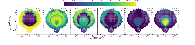
(a) M08_03

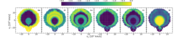
(b) M10_03

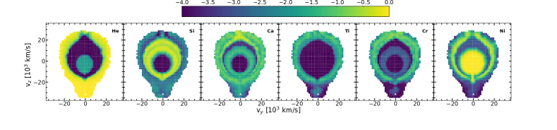
(c) M10_05

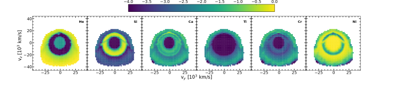
(d) M10_10

Figure 1: Colour scale indicates the abundances in log mass fraction of key species for selected models. Included are models showing a secondary detonation by the converging shock (M08_03), scissors (M10_05) and edge-lit (M10_10) mechanisms.

Table 1: Model parameters. Model masses listed are pre-relaxation (see Gronow et al. (2021) for details). We keep the model names from Gronow et al. (2021). We include the abundances of ⁵⁶Ni synthesised in each model since this predominantly determines the model light curve brightness. For other nucleosynthetic abundances see Gronow et al. (2021). We show the ignition mechanism of the secondary detonation, which are the converging shock mechanism ‘cs’; the scissors mechanism ‘s’; the converging shock mechanism, but with carbon burning at the convergence of the helium detonation, similar to the scissors mechanism ‘(s,)cs’; and the edge-lit mechanism ‘edge’. We note that in Model M10_02 the secondary detonation due to the converging shock was artificially ignited by hand. Also shown are the angle-averaged peak light curve brightnesses, as well as time of peak, and the decline rate in B band over 15 days from peak, $\Delta$m₁₅(B).

	M08_03	M08_05	M08_10_r	M09_03	M09_05	M09_10_r	M10_02	M10_03	M10_05	M10_10	M11_05
Core Mass [M⊙]	0.803	0.803	0.795	0.905	0.899	0.888	1.005	1.028	1.002	1.015	1.100
Shell Mass [M⊙]	0.028	0.053	0.109	0.026	0.053	0.108	0.020	0.027	0.052	0.090	0.054
56Ni Core [M⊙]	$1.3\times 10^{-1}$	$2.0\times 10^{-1}$	$3.1\times 10^{-1}$	$3.3\times 10^{-1}$	$3.8\times 10^{-1}$	$4.8\times 10^{-1}$	$5.4\times 10^{-1}$	$5.9\times 10^{-1}$	$5.4\times 10^{-1}$	$7.2\times 10^{-1}$	$8.3\times 10^{-1}$
56Ni Shell [M⊙]	$9.9\times 10^{-7}$	$6.7\times 10^{-5}$	$1.5\times 10^{-2}$	$1.0\times 10^{-6}$	$2.0\times 10^{-3}$	$2.6\times 10^{-2}$	$1.9\times 10^{-6}$	$6.0\times 10^{-5}$	$8.2\times 10^{-3}$	$3.9\times 10^{-2}$	$1.2\times 10^{-2}$
Mechanism	cs	(s,) cs	s	(s,) cs	(s,) cs	s	art cs	(s,) cs	s	edge	edge
Mbol,max	-17.6	-17.9	-18.4	-18.4	-18.5	-18.8	-18.9	-19.0	-18.9	-19.2	-19.3
MU,max	-16.3	-16.7	-17.5	-17.8	-17.9	-18.7	-18.9	-19.0	-18.9	-19.2	-19.4
MB,max	-17.0	-17.2	-18.0	-18.3	-18.3	-18.9	-19.0	-19.2	-19.0	-19.4	-19.6
MV,max	-18.3	-18.6	-19.2	-19.3	-19.4	-19.7	-19.7	-19.8	-19.7	-20.1	-20.1
MR,max	-18.4	-18.8	-19.2	-19.1	-19.3	-19.4	-19.4	-19.5	-19.4	-19.6	-19.6
tbol,max [days]	17.4	18.1	17.9	18.1	18.1	17.2	17.3	17.1	17.4	16.6	16.1
tU,max [days]	15.1	16.4	16.4	15.7	16.7	15.6	15.1	15.2	16.0	14.3	13.8
tB,max [days]	17.5	17.8	17.8	18.0	18.1	17.2	17.2	16.9	17.4	16.3	15.6
tV,max [days]	19.2	19.9	19.5	19.9	19.9	19.0	19.6	19.4	19.5	18.7	18.6
tR,max [days]	18.3	19.2	17.5	18.0	18.0	16.7	17.6	17.4	17.2	16.7	16.7
$\Delta\mathrm{m}_{15}$(B)	1.38	1.54	1.94	1.52	1.96	2.01	1.51	1.73	1.94	1.42	1.35

We carry out radiative transfer simulations for the 3D hydrodynamical explosion simulations by Gronow et al. (2021). They investigated 11 models with a range of different core and shell masses. The model core masses range from 0.8 M_⊙  to 1.1 M_⊙  and the shell masses range from 0.02 M_⊙  to 0.1 M_⊙. The shell and core mass combinations were chosen to match models in previous work (eg. Woosley & Kasen, 2011; Polin et al., 2019; Townsley et al., 2019). A core mass of $\sim$ 1 M_⊙  has been found to produce models of similar brightness to normal SNe Ia (eg. Sim et al., 2010; Kromer et al., 2010). Given that the initial model masses vary significantly between models, parameters important for determining the evolution of the explosion, such as the central density, also vary between models. In all models, a helium detonation is ignited at a point on the positive $z$-axis in the helium shell, as was described by Gronow et al. (2021). Three different mechanisms were found to ignite the secondary core detonation, and one model did not dynamically ignite a secondary detonation. The three mechanisms were the converging shock (eg. Livne, 1990; Fink et al., 2007; Shen & Bildsten, 2014), edge-lit (eg. Livne & Glasner, 1990) and scissors mechanism (Forcada et al., 2006; Gronow et al., 2020; Gronow et al., 2021). The explosion mechanism for each model is listed in Table 1. Following Gronow et al. (2021), the models are named indicating the original masses of the core and shell, which are listed in Table 1. Figure 1 indicates the relative abundances of key species in the ejecta for models showing each of the three detonation mechanisms found in this study. All three mechanisms produce highly asymmetrical ejecta, as has previously been discussed by Gronow et al. (2021).

3 Results

We have computed the light curves and spectra for each of the explosion models. We first present the light curves in Section 3.1, and then present the spectra in Section 3.2.

3.1 Light curves

In this section, we discuss the light curves predicted for the models presented by Gronow et al. (2021). We first present the angle-averaged properties of the light curves in Section 3.1.1 and their colour evolution in Section 3.1.2. We then discuss the viewing-angle dependence of the light curves in Section 3.1.3. We compare the light curves to the normal SN 2011fe (Nugent et al., 2011), the over-luminous SN 1991T (Filippenko et al., 1992) and the sub-luminous SN 1999by (Garnavich et al., 2004) to determine the ability of these models to reproduce the main classes of observed SNe Ia, and also compare to the sample of observed SNe Ia from Hicken et al. (2009).

3.1.1 Angle-averaged light curves

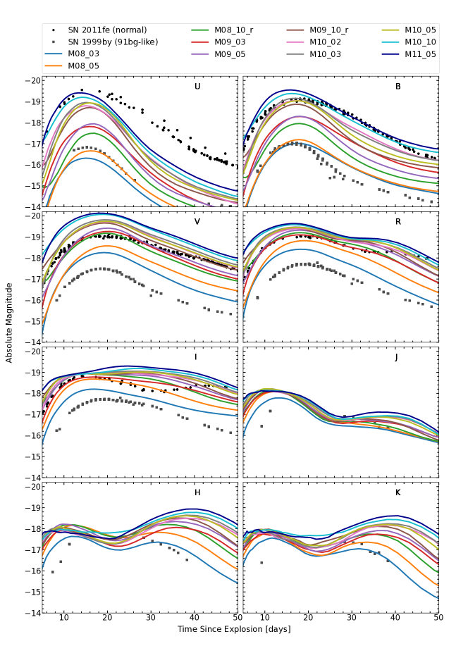
Figure 2: Angle-averaged band limited light curves for our parameter study models. Also plotted are the light curves of the normal SN 2011fe and 91bg-like SN 1999by.

To make general comparisons between the models, we first discuss the angle-averaged light curves. As indicated by the asymmetries in the explosion ejecta (see Figure 1), the angle-averaged light curves do not give a complete representation of the models as a whole. We discuss the line of sight dependent light curves in Section 3.1.3.

In Figure 2 we show the band limited angle-averaged light curves for each of the models. We also show the light curves of the normal SN 2011fe, and the 91bg-like SN 1999by to indicate the fainter end of observed SNe Ia. As anticipated from the range of model masses, specifically the range in masses of ⁵⁶Ni synthesised in the models (see Table 1), the light curves show a wide range of brightnesses. These span from fainter, 91bg-like brightnesses to normal brightness SNe Ia, as previously discussed by Gronow et al. (2021) for the model bolometric light curves. Interestingly, the increase in model mass from M10_10 to M11_05 does not show a significant increase in light curve brightness. This may indicate that this scenario does not explain the brightest observed SNe Ia. Since increasing model mass increases the central density, leading to higher abundances of Fe-group material and lower abundances of IME’s, increasing the model mass further to increase the brightness will lead to an over-production of Fe-group elements.

In this work, we do not present the early light curve evolution (< 5 days), since very early times are computationally expensive. However, we note that particularly the massive He shell models tend to show an excess of flux in the bluer bands at early times, similar to that found by Noebauer et al. (2017), due to the surface radioactive material synthesised during the He shell detonation.

Compared to observations, the models tend to be too faint in the U band and too bright in V band, such that the models are redder than observations. We discuss the model colour evolution in Section 3.1.2. In agreement with SN 1999by, our faintest models (Models M08_03 and M08_05) do not show secondary maxima in the R and I bands. While our brightest models do show secondary maxima (in agreement with normal SNe Ia), they do not match the times of the secondary maxima in SN 2011fe. The NIR secondary maxima in SNe Ia are attributed to the recombination of doubly ionised iron group elements to singly ionised in the inner iron-rich regions of the ejecta (Kasen, 2006; Kromer & Sim, 2009; Jack et al., 2015), as the ejecta expands and cools. When this occurs, the flux from the UV and blue parts of the spectrum is most effectively redistributed to the red and near-infrared by fluorescence, causing the secondary maxima. It is likely that the temperature in the ejecta is underestimated in our simulations, since we do not include a full non-LTE solution (see discussion in Section 3.1.2). Therefore it is plausible that this is the reason that our secondary maxima in the R band occur too early.

3.1.2 Angle-averaged colour evolution

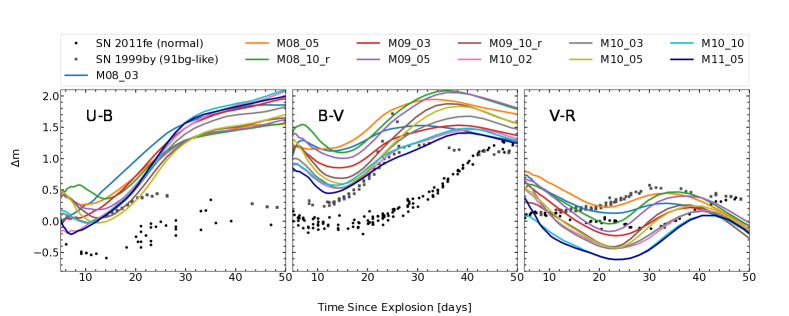
Figure 3: Angle-averaged U-B, B-V, and V-R colour evolution of our models. The colours of the normal SN 2011fe and 91bg-like SN 1999by are also plotted.

As previously discussed, many recent double detonation models show B$-$V colours too red compared to observations (Kromer et al., 2010; Woosley & Kasen, 2011; Polin et al., 2019; Gronow et al., 2020; Shen et al., 2021b). This is predominantly due to line blanketing caused by heavy elements in the outer layers of the ejecta, synthesised in the helium detonation. Townsley et al. (2019), however, do not find these extremely red colours for their minimal helium shell mass model, and Shen et al. (2021b) also find their minimal mass helium shell models do not show such red colours.

Our model shell masses range from a minimal shell mass of $0.02$ M_⊙  (Model M10_02) to thicker shell masses of $\sim 0.1$ M_⊙. Compared to early double detonation models, this is still a low helium shell mass (e.g. Nugent et al. 1997 considered a helium shell mass of $0.2$ M_⊙). In Figure 3 we plot the angle-averaged colour evolution for each of the models. We discuss colour in specific lines of sight in Section 3.1.6.

Generally, colour evolution is a temperature effect, such that brighter, hotter SNe Ia show bluer colours than fainter, cooler SNe Ia (e.g. Tripp 1998). We do find this general trend for our models, such that brighter models tend to show bluer colours, however, none of our angle-averaged light curves show B-V colours similar to observed normal SNe Ia with similar peak brightness, as the colours are extremely red. Even our lowest shell mass model M10_02 shows B-V colours significantly redder than the normal SN 2011fe. Therefore we do not confirm the results of Townsley et al. (2019) and Shen et al. (2021b) that a minimal helium shell mass leads to normal SNe Ia colours.

Similarly, the U-B model colours do not reproduce those expected for normal SNe Ia, due to line blanketing of the spectra at these wavelengths, caused by the heavy elements synthesised in the helium shell detonation. The V-R colours are more similar to those of normal SNe Ia than the bluer bands. As indicated by the light curves, these bands are not as strongly affected by the excess absorption caused by the burning products of the helium shell detonation. However, we still do not find the expected V-R colour evolution. This is likely in part due to the predicted timing of the R band secondary maxima, as discussed in Section 3.1.1.

It may be that ionisation effects are contributing to the redness of the models, as a result of the assumptions made in the radiative transfer calculations in artis (i.e. not solving the full non-LTE equations of statistical equilibrium). Full non-LTE simulations of sub-${\rm{M}}_{\rm{ch}}$, helium ignited models were found to be very blue at maximum light in non-LTE simulations by Höflich & Khokhlov (1996) and Nugent et al. (1997). Similar results were found by Blondin et al. (2017), who found that their non-LTE simulations of sub-${\rm{M}}_{\rm{ch}}$, pure detonation (i.e. no helium shell) models showed similar colours to observations, and for fainter models, even bluer colours than similar brightness ${\rm{M}}_{\rm{ch}}$ models. Shen et al. (2021a) also found that their non-LTE, pure-detonation models were more highly ionised than LTE simulations after maximum light, and showed less Fe ii absorption. At B-band maximum light, the greatest difference in B-V colour of their non-LTE simulations was $\sim 0.25$ mag bluer than their LTE simulation. However, at 15 days after maximum light, the maximum difference in B-V colour of the non-LTE simulation was $\sim 1$ mag bluer than the LTE simulation. The maximum light B-V colour of our least red model (M11_05) is 0.5 mag, while SN 2011fe has a B-V $\approx$ 0 mag at maximum light. Therefore, a more accurate, full non-LTE treatment of the radiative transfer may reduce the apparent discrepancies between our double detonation model colours and observations, but is unlikely to fully reconcile the discrepancy. In addition, we note that the full non-LTE simulation of a helium detonation model, with no secondary core detonation, presented by Dessart & Hillier (2015) still showed red colours, despite the non-LTE treatment.

3.1.3 Line of sight dependent light curves

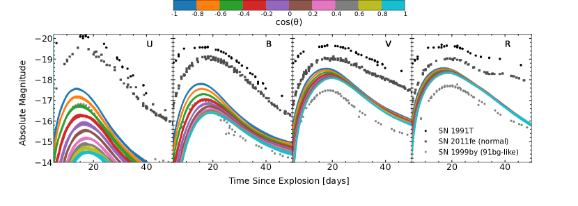
(a) M08_03

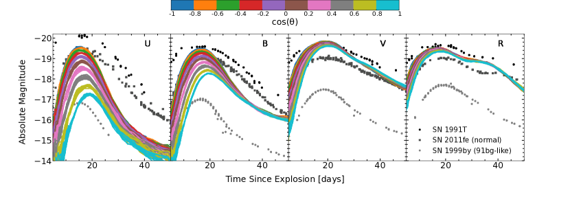
(b) M10_05

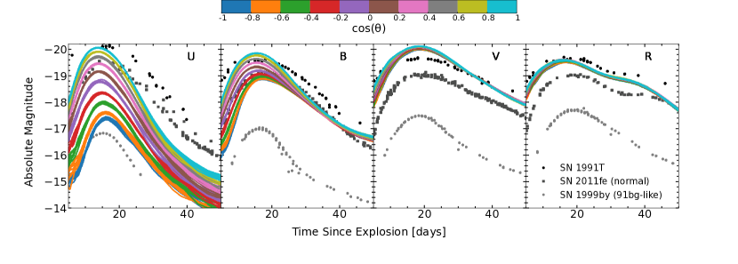
(c) M10_10

Figure 4: Light curves of Models M10_10, M10_05 and M08_03, where escaping Monte Carlo packets (representing packets of photons) have been binned in 10 equal solid-angle bins in cos($\mathrm{\theta}$), indicated by the colour coding, and for each angle bin in cos($\mathrm{\theta}$) there are 10 equal solid-angle bins in $\mathrm{\phi}$. Since the models are close to asymmetric, we do not find significant variation in $\mathrm{\phi}$. The U and B bands show a strong angle dependence in cos($\mathrm{\theta}$), which becomes less significant with time as the ejecta become more optically thin.

In this section we discuss the light curves produced in different lines of sight. We show light curves for 100 viewing angles, where escaping Monte Carlo packets are divided into equal solid-angle bins (i.e. binned on a uniform grid in cos($\theta$) and $\phi$, where $\theta$ and $\phi$ are the usual spherical polar angles).

In Figure 4, we plot the viewing-angle dependent light curves for Models M08_03, M10_05 and M10_10. Each of these models showed a different mechanism to ignite the secondary core detonation; converging shock, scissors mechanism and edge-lit, respectively. The ejecta composition for these models is shown in Figure 1. The U and B band light curves show an extremely strong viewing-angle dependence. The strong viewing-angle dependence in double detonation models has previously been discussed (e.g. Kromer et al., 2010; Gronow et al., 2020). The dependence is due to a combination of line blanketing effects, as well as the distribution of ⁵⁶Ni within the model ejecta. For example, in Models M10_05 and M08_03, in the southern hemisphere the ⁵⁶Ni is nearer to the surface of the ejecta, leading to brighter and earlier maxima in the bluer bands. This effect of the distribution of ⁵⁶Ni in the model has previously been discussed by Sim et al. (2012). In the northern hemisphere, the ⁵⁶Ni is further from the ejecta surface, which leads to fainter light curves in these lines of sight. In addition to this, higher abundances of heavy elements (such as Ti, Cr and Fe-group elements) are synthesised in these lines of sights in the outer ejecta, leading to stronger absorption in the bluer bands, and in the extreme cases near the pole, leads to line blanketing of blue wavelengths. The reverse is true for Model M10_10, which was ignited by the edge-lit mechanism. In this case the ⁵⁶Ni is nearer the surface in the northern hemisphere (see Figure 1), resulting in these lines of sight showing the brightest light curves. Despite this reversal, the viewing angle dependence shown by this model is similar to the level shown by Model M10_05.

The viewing angle dependence shown by the models is not as strong in the redder bands, as can be seen in the V and R bands in Figure 4. We also note that in the bluer bands the viewing angle dependence decreases over time. This can be understood by the ejecta becoming more optically thin over time, leading to the reduced viewing angle dependence.

3.1.4 Width-luminosity relation

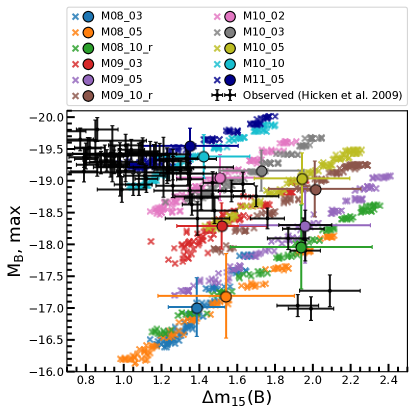
Figure 5: Peak B band magnitude plotted against $\Delta$m₁₅(B) for the angle-averaged light curve values (circles) and 100 different viewing angles (x) for each model, compared to a sample of observed SNe Ia from Hicken et al. (2009). SNe Ia with a distance modulus $\mu<33$ have been excluded. The error bars show the standard deviation of the viewing angle distributions.

It has previously been shown that sub-${\rm{M}}_{\rm{ch}}$ white dwarfs show reasonable agreement with the observed width-luminosity relation (Sim et al., 2010; Blondin et al., 2017; Shen et al., 2018, 2021a) shown by SNe Ia (Phillips, 1993). This relation can be seen in Figure 5, showing the observed sample of SNe Ia from Hicken et al. (2009). Chandrasekhar mass models for SNe Ia generally fail to reproduce the full width-luminosity relation, such that models can not explain observations with $\Delta$m₁₅(B) $\gtrsim 1.5$ (Kasen et al., 2009; Sim et al., 2013; Blondin et al., 2017). Sub-${\rm{M}}_{\rm{ch}}$ models, however, have been shown to explain the fainter, faster evolving end of the width-luminosity relation (Sim et al., 2010; Blondin et al., 2017; Shen et al., 2018, 2021a). The variation in mass readily explains the variation in the amount of ⁵⁶Ni synthesised, and therefore the variation in observed peak brightness. Most previous studies investigating the width-luminosity relation for sub-${\rm{M}}_{\rm{ch}}$ explosion models have considered bare carbon-oxygen white dwarfs as the explosion models, and therefore did not consider the mechanism responsible for igniting the detonation. Here we investigate whether double detonation models can also explain the variation shown by the width-luminosity relation. In Figure 5, we plot B band maximum against $\Delta$m₁₅(B) for each model line of sight, as well as the angle-averaged values. The models indeed show decline rates $\Delta$m₁₅(B)$\gtrsim 1.5$, and the angle averaged points in Figure 5 generally lie close to the observed SNe Ia. However, the extent of the viewing angle dependence is much greater than that shown by the observational data. Gronow et al. (2021) similarly found that the bolometric light curves showed a greater viewing angle dependence than the bolometric dataset of SNe Ia of Scalzo et al. (2019). Our models, however, do not account for the brighter end of the observed width-luminosity relation, showing slower decline rates (see Figure 5).

Despite the observed width-luminosity relation being a characteristic feature of SNe Ia, the physical reason for the observed trend is not yet fully understood, or entirely reproduced by simulations. The B band width-luminosity relation is dependent on the diffusion time, but also on the colour evolution of SNe Ia (Kasen & Woosley, 2007). Simulations of colour evolution are particularly uncertain, especially in the bluer bands, since transitions at these wavelengths are extremely sensitive to the micro-physics describing the state of the gas. Therefore, to simulate the colour evolution, we must have a good description of e.g. ionisation, excitation and temperature of the ejecta. It is likely that the width-luminosity relation of our models is sensitive to non-LTE effects, and therefore future full non-LTE simulations may show better agreement with observations.

In addition to the challenges of simulating colour evolution, artis, and other codes that do not include full non-LTE treatments, (see e.g. Shen et al. 2018) tend to overestimate the decline rate. Therefore it is possible that these explosion models would show a slower decline from maximum if we included a full non-LTE treatment, e.g. Shen et al. (2021a) found their non-LTE models showed a slower B-band decline rate than their LTE simulations (a maximum difference of $\Delta$m₁₅(B) $=1$ mag). Full non-LTE simulations are required to quantify this effect for double detonation simulations. Blondin et al. (2017) use the non-LTE radiative transfer code cmfgen, and find that the sub-${\rm{M}}_{\rm{ch}}$ models they consider are able to reproduce the full width luminosity relation with sub-${\rm{M}}_{\rm{ch}}$ explosion models. Similar results were found by Shen et al. (2021a). These, however, did not consider the ignition mechanism, and therefore did not suffer from the apparent problems introduced by the helium shell detonation, and were also 1D and neglected potential viewing-angle dependencies. Future work should investigate the effect of full non-LTE simulations on the width-luminosity relation for double detonation simulations.

The lowest mass models in our study (M08_03 and M08_05) show similar B band peak brightnesses to faint, 91bg-like objects, which have peak magnitudes of $\sim-17$ mag. They do not, however, account for the decline rates of 91bg-like objects of $\sim 1.9$ (see Figure 5). Models M08_03 and M08_05 do not follow the observed width luminosity relation. Gronow et al. (2021) also found that these two models did not agree with observations in bolometric light. This is in agreement with Blondin et al. (2017), who found that their low mass (0.88 M_⊙) 1D bare white dwarf detonation model showed an anti-width luminosity relation. Shen et al. (2018) and Polin et al. (2019) have also noted this, and following discussion by Shen & Bildsten (2014), they suggest that this may be due to a physical minimum white dwarf mass, associated with the central density that can be ignited via the converging shock mechanism.

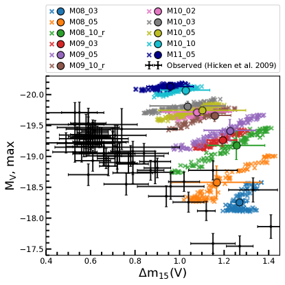
Figure 6: V-band width luminosity relation. Circles show the angle-averaged values while crosses show values in individual lines of sight. The error bars on the models show the standard deviation of the viewing angle distribution. Also plotted is the sample from Hicken et al. (2009).

Since the B-band light curves are particularly strongly impacted by absorption from the helium shell detonation ash, we also show the V-band width luminosity relation for our models in Figure 6, and compare this to observations. As expected from the light curves, the viewing angle dependence is not as strong in V-band, particularly for the brighter models. However, we note that our V-band light curves appear to be too bright compared to observations in Section 3.1.1, and this can be seen in Figure 6. The V-band decline is also too fast compared to observations, such that we find a systematic offset between models and observations.

3.1.5 Rise time

Figure 7: Time taken to reach B-band maximum light from the time of explosion, plotted against peak absolute magnitude in B-band. We show the rise time for the angle-averaged light curves (circles) as well as in each line line of sight (x). The error bars show the standard deviation of the viewing angle distributions.

In Figure 7 we show the time taken from explosion for each model to reach maximum light on average and in each line of sight. Brighter models tend to show a faster rise-time to maximum light, except for the faintest part of our model range. The average rise time of our models ranges from 15.7 to 18.1 days. Apart from Model M11_05, which showed the fastest rise time, this is in agreement with rise times found for SNe Ia by Firth et al. (2015) ranging from 15.98 to 24.7 days. Particularly in the faster rising lines of sight, Model M11_05 shows rise times too fast compared to observations. The variation in rise-time found in each line of sight is primarily driven by the distribution of ⁵⁶Ni in the ejecta, such that lines of sight where the ⁵⁶Ni is nearer the surface show a faster rise to maximum. This can also be seen in Figure 4 showing line of sight dependent model light curves.

3.1.6 B-V colour at B band maximum

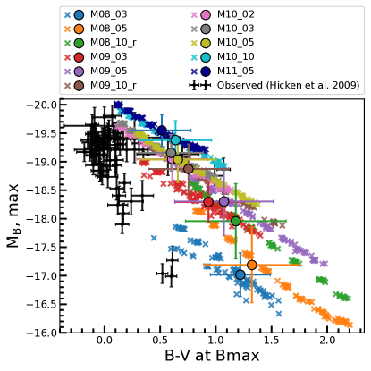
Figure 8: B-V colour at B max for each line of sight, plotted against B band maximum. Also plotted is the observed sample from Hicken et al. (2009). All of the models are too red compared to observations.

In Figure 8 we show the B-V colour at the time of B band maximum for each of the 100 different viewing-angles in the 3D models. Again this highlights the extent of the viewing angle dependence in our set of double detonation simulations. We also show the colour of a sample of normal SNe Ia from Hicken et al. (2009). It is clear from this that all of our models are too red compared to normal SNe Ia. In the brighter, more massive models, the brightest lines of sight lie within the range of observations, however overall, even for these models, the colours are too red. This includes our model with the lowest mass helium shell, Model M10_02. As previously discussed, light curve colour is challenging to simulate, given the dependence of wavelength on the conditions in the ejecta, such as temperature, ionisation and excitation state, as well as dependence on the atomic data included in the calculation. In particular, the bluer bands are sensitive to this, given the number of transitions at these wavelengths. The large abundances of heavy elements produced in the outer ejecta layers in the helium detonation cause strong absorption of bluer wavelengths in our simulations, leading to the extremely red colours. However, this absorption may be exaggerated by the approximations made in the treatment of ionisation in our radiative transfer calculations. We note that colours redder than observations have previously been found by artis for other classes of explosion models, including delayed-detonation models (Sim et al., 2013) and pure detonations (Sim et al., 2010), however, these colours were only slightly redder than observations (B-V at maximum $\approx 0.5$ for the reddest models), and not the extremely red colours found here. Full non-LTE simulations are required to fully investigate the B-V colour of these double detonation models, and determine whether this is a problem with the explosion scenario, or due to shortcomings in the radiative transfer simulations.

3.2 Spectra

In this section we present the model spectra. We first discuss the angle-averaged spectra in Section 3.2.1, and then make comparisons of the line of sight spectra to observations in Sections 3.2.2 and 3.2.3.

3.2.1 Angle-averaged spectra

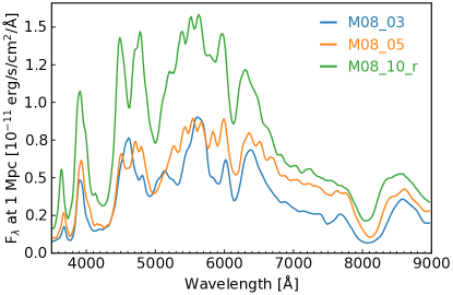
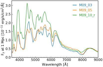
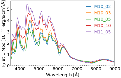
Figure 9: Angle-averaged model spectra at 2 weeks after explosion.

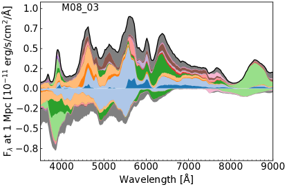
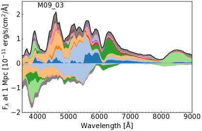
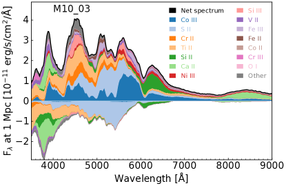
Figure 10: Spectra at 2 weeks after explosion for each of the models with helium shells of $\sim$ 0.3 M_⊙, where the contributions by individual ions to the spectra are indicated. Beneath the axis we also indicate the ions responsible for absorption. These can be directly compared to Figure 9.

We show the model angle-averaged spectra at two weeks after explosion in Figure 9, and compare models with similar total masses. All of the spectra show characteristic IME spectral features, including Si ii $\lambda 6355$, S ii $\lambda\lambda 5454,5640$ and the Ca ii triplet at $\lambda\lambda$8498, 8542, 8662. However, despite relatively low masses of Ti in our models, all of the model spectra show a clear absorption feature at $\sim$ 4000–4500 Å, dominated by Ti ii absorption. Such a feature is observed in sub-luminous, 91bg-like SNe Ia, due to the lower temperatures, and therefore lower ionisation state of the ejecta (Mazzali et al., 1997), but is not observed in normal SNe Ia. We note however that such a feature has been observed in the normal brightness, peculiar SN 2016jhr (Jiang et al., 2017), and shows good agreement with the spectral features predicted for the double detonation Model M2a of Gronow et al. (2020), which is similar to Model M10_05. The prediction of a Ti ii absorption feature for the double detonation is in agreement with the previous findings of Kromer et al. (2010), Townsley et al. (2019) and Gronow et al. (2020). As model mass decreases, and therefore as model brightness decreases, we find stronger Ti ii absorption and redder colours. Since the lower mass models tend to have higher abundances of Ti, and on average lower temperatures and ionisation states, this is to be expected.

Even our lowest helium shell mass model (M10_02) shows a clear Ti ii absorption feature, which is similar in strength to the Ti ii feature predicted for models M10_03 and M10_05 (see Figure 9). Townsley et al. (2019) have suggested that thin helium shells of similar mass to that in Model M10_02 can produce spectra of normal SNe Ia, however, we find that even our lowest helium shell mass model still predicts spectra that would be classified as a peculiar SN Ia. In Figure 10 we indicate the key ions contributing to the emission spectrum for each of Models M10_03, M09_03 and M08_03 at 2 weeks after explosion, and also indicate the species responsible for absorption (shown beneath the axis).

3.2.2 Viewing-angle dependent spectra

As demonstrated in Section 3.1.3, the models show strong viewing-angle dependencies, particularly at bluer wavelengths, where the products of the helium shell detonation most strongly affect the spectrum. We now discuss the viewing-angle dependence shown by the spectra.

Figure 11 shows spectra in specific lines of sight for Model M10_03. As expected, given the asymmetries shown by the light curves, the spectra at 2 weeks after explosion show a strong viewing angle dependence. Lines of sight viewing towards the northern pole, where the helium detonation was ignited at cos($\theta$) = 1, show extreme line blanketing at blue wavelengths, as has previously been discussed by Kromer et al. (2010) and Gronow et al. (2020). In these lines of sight, high abundances of heavy elements were produced in the helium shell detonation, such as Cr, Ti and Fe-peak elements. These elements are extremely effective at line blanketing. In addition to the high abundances of heavy elements, the ⁵⁶Ni was produced farthest from the surface in these lines of sight. Therefore it is not unexpected that the spectra in these lines of sight are fainter, however, consequently, these are also the coolest and least ionised, which has the effect of increasing the level of line blanketing. We note that redder wavelengths do not show a strong viewing angle dependence, except for the Ca ii triplet, which we find to be stronger and at higher velocities in lines of sight near cos($\theta$) = 1.

In Figure 11, we also plot spectra of the normal SN Ia, SN 2011fe, at similar epochs. At each epoch our model spectra produce characteristic SNe Ia features, such as Si ii $\lambda$6355 and S ii $\lambda\lambda 5454,5640$. However, in all lines of sight the spectra are much redder than the spectra of SN 2011fe, which represents a typical ‘normal’ Type Ia SN. Additionally, the model Si ii $\lambda$6355 features are produced at higher velocities than the observations. We note that the spectra of Model M10_02 are similar to model M10_03.

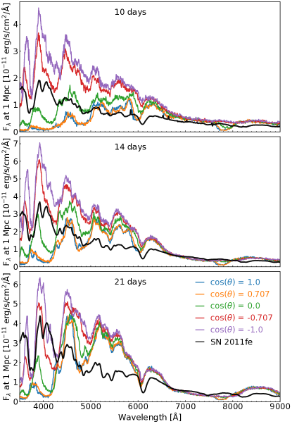
Figure 11: Spectra in specific lines of sight of Model M10_03. These were calculated using ‘virtual packets’. We compare the model spectra to SN 2011fe at similar epochs.

3.2.3 Line of sight spectra compared to SN 2018byg

SN 2018byg was suggested by De et al. (2019) to be the result of a double detonation. The bluer regions of the spectra of SN 2018byg showed unusually strong line blanketing, with broad Ti ii and Fe-group element absorption features, and near peak a deep, high velocity ($\approx$ 25 000 km s^-1) Ca ii triplet absorption feature was observed. The light curves of SN 2018byg are subluminous and similar to SN 1991bg-like SNe Ia, except for a rapid rise in r-band magnitude within the first week from explosion. Gronow et al. (2020) compared the level of absorption in the faintest lines of sight in their reference model, M2a, to the absorption shown by SN 2018byg, and found that this was a good match to the level of line blanketing observed. However, Model M2a showed light curves brighter than those observed for SN 2018byg. We now make this comparison with a model showing peak brightnesses similar to SN 2018byg, which had a peak absolute magnitude of M${}_{\mathrm{R,max}}\approx-18.2$ mag (De et al., 2019). This is similar to Model M08_03 which showed M${}_{\mathrm{R,max}}=-18.4$ mag.

In Figure 12 we show the spectra of M08_03 compared to spectra of SN 2018byg at similar epochs. At 10 days after explosion, the model line of sight at cos($\theta$)$=-0.707$ is similar to SN 2018byg, however, by 14 days after explosion, SN 2018byg shows stronger line blanketing and more closely resembles the lines of sight at cos($\theta$)$=1$ and cos($\theta$)$=0.707$. By 17 days after explosion the model no longer shows strong enough line blanketing to explain that in SN 2018byg.

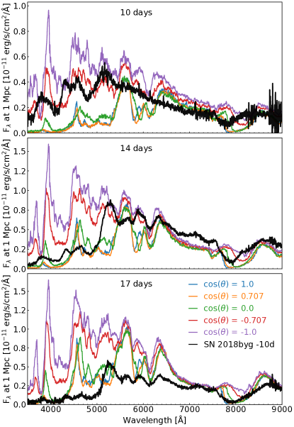
Figure 12: Spectra of Model M08_03 in specific lines of sight at 10, 14 and 17 days after explosion. Also shown are the spectra of SN 2018byg at similar epochs.

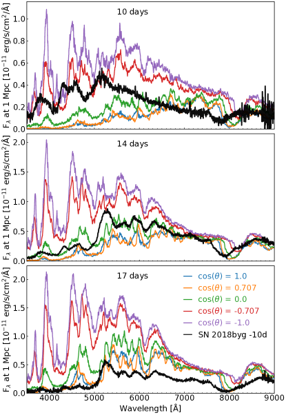
Figure 13: Same as Figure 12, but compared to the spectra of Model M08_05.

Since the model with the lower shell mass does not account for the line blanketing in SN 2018byg, we compare SN 2018byg to Model M08_05 in Figure 13. The angle-averaged peak R band magnitude of Model M08_05 is M${}_{\mathrm{R,max}}=-18.8$, although the faintest lines of sight have M${}_{\mathrm{R,max}}=-18.6$. The R band light curves in our models do not show as strong an angle dependence as shown by the bluer bands (see Figure 4). We find that the more massive He shell of Model M08_05 is able to account for the line blanketing observed in SN 2018byg. At redder wavelengths, however, Model M08_05 is brighter than SN 2018byg. Therefore it is possible that a lower mass core might be able to better account for SN 2018byg. We also compared the line of sight spectra for Model M08_10 to SN 2018byg, and found that the spectrum in the faintest line of sight is able to account for the line blanketing in SN 2018byg, however, the model spectrum is too bright at redder wavelengths, and does not account for the broad Ca ii absorption feature.

This suggests that the mass of the He shell of SN 2018byg could have been similar to Model M08_05. This is a significantly lower shell mass than suggested by De et al. (2019) for SN 2018byg: De et al. (2019) suggest that a He shell mass of $\approx 0.15$ M_⊙ is required to explain the observed properties of SN 2018byg, whereas the shell mass of Model M08_05 was 0.053 M_⊙ (pre-relaxation; see Gronow et al. 2021 for the definition of the He shell mass after mixing was allowed to take place).

4 Discussion and conclusions

We have carried out radiative transfer simulations for a series of simulations by Gronow et al. (2021) of the double detonation explosion scenario, where the initial core and helium shell masses were varied.

The variation in model mass produced a range of masses of ⁵⁶Ni, and therefore the simulated light curves for these models showed a range of peak brightnesses. The brightnesses shown by the light curves were able to account for normal SNe Ia, as well as fainter 91bg-like SNe. However, in agreement with previous works, the colours are much redder than observed for normal SNe Ia for all of our models, due to strong absorption features by heavy elements produced in the outer ejecta during the helium shell detonation. Townsley et al. (2019) and Shen et al. (2021b) found that minimal helium shell models are able to produce normal SNe Ia, however, our minimal helium shell model, M10_02, still shows colours too red. This shows that even low masses of He detonation ash can be significant enough to affect the model colours.

The double detonation explosion models showed strong asymmetries, which seem to be in conflict with the tight relationship shown by the Phillips relation. All three secondary detonation mechanisms found in this study (converging shock, scissors and edge-lit mechanisms) produced similarly asymmetric ejecta. The bluer band light curves showed an extremely large viewing angle dependence. These wavelengths showed strong absorption and line blanketing in some lines of sight, due to the helium shell burning products. The redder bands, however, did not show such strong asymmetries. We also found that over time the light curves became less angle dependent as the ejecta became more optically thin.

In agreement with previous studies of sub-${\rm{M}}_{\rm{ch}}$ explosions (Sim et al., 2010; Blondin et al., 2017; Shen et al., 2018, 2021a), the models show variation in decline rate with peak brightness, which are able to reproduce the overall trend of the faint end of the width luminosity relation. However, they do not reproduce the bright end of the width luminosity relation. It is possible that future, full non-LTE simulations may change the predicted decline rates, since the flux in the B band is sensitive to ionisation state, and it is likely that our approximate non-LTE treatment underestimates the ionisation at later times. Simulations by Shen et al. (2021a) of sub-${\rm{M}}_{\rm{ch}}$ explosion models indicate that the decline rate is affected by considering non-LTE (a slower decline rate of up to $\Delta$m₁₅(B) $=1$ mag for their non-LTE simulation compared to LTE).

We also find that the viewing angle dependence in the width-luminosity shown by the models is stronger than is observed. The asymmetry of the models is predominately in the helium shell detonation ash. If the radiative transfer effects from the helium shell were reduced, e.g. by considering an even thinner He shell than Model M10_02, or through ionisation effects, it is possible that the models would not show such strong asymmetries.

All of our model spectra show signatures of the helium shell detonation products, particularly Ti ii, that are not observed in normal SNe Ia. This includes the minimal He shell mass model, M10_02. Similarly to Kromer et al. (2010) and Gronow et al. (2020), the spectra show a strong viewing angle dependence. Lines of sight opposite to the ignition point of the helium detonation show strong absorption features, particularly at blue wavelengths, due to the helium shell detonation products, which have the highest abundance in these lines of sight. Additionally, the ⁵⁶Ni produced in the CO core detonation is furthest from the surface of the ejecta in these lines of sight, and as a result these are cooler than lines of sight where the ⁵⁶Ni from the core detonation is closer to the surface. Therefore the products of the helium shell detonation are less ionised and cause stronger absorption features. It is possible that such lines of sight could explain peculiar SNe Ia, such as SN 2018byg, which showed strong line blanketing in its spectra. The level of line blanketing observed can be explained by our models with similar peak brightness.

For double detonations to be able to explain normal SNe Ia, the effects of the helium shell detonation need to be minimised. Pure detonation models (where the CO core is detonated without a helium shell) show good agreement with observations (e.g. Sim et al. 2010; Blondin et al. 2017; Shen et al. 2018, 2021a), and double detonation explosion simulations with the helium detonation ash removed (e.g. Kromer et al. 2010; Pakmor et al. 2022) show similarly good agreement with observations, and would no longer be classified as peculiar SNe Ia. Although our lowest mass helium shell model does not reproduce normal SNe Ia, Townsley et al. (2019) and Shen et al. (2021b) have shown that their low mass helium shell models are able to better reproduce normal SNe Ia. The $1.0$M_⊙, $\rho_{5}=3$ model by Boos et al. (2021), considered by Shen et al. (2021b), and the model by Townsley et al. (2019) are similar to our Model M10_02. In Table 2 we compare the masses of ⁴⁴Ti and ⁴⁸Cr produced in the helium shell detonations for these models. Our Model M10_02 has the highest abundances of these species produced in the shell detonation, which is likely the primary reason for the differences in colour found in our simulations. The Boos et al. (2021) $1.0$M_⊙, $\rho_{5}=3$ model uses the same model as Townsley et al. (2019) (initial parameters, enrichment, and nuclear reaction network). However, for modelling the detonations Boos et al. (2021) used a burning limiter while Townsley et al. (2019) did not. This may point to the treatment of the He detonation in the explosion simulations as the reason for the differences in abundances. To investigate this, the He detonation should be spatially resolved, which is within reach for future simulations but beyond the scope of this work.

Table 2: Masses of ⁴⁴Ti and ⁴⁸Cr produced in the helium shell detonation for our Model M10_02, the 1.0 + 0.02 M_⊙  model by Townsley et al. (2019) and the $1.0$ M_⊙, $\rho_{5}=3$ from Boos et al. (2021) and Shen et al. (2021b). For similar initial CO core and He shell masses our model produces the highest abundances of ⁴⁴Ti and ⁴⁸Cr in the shell detonation. These species are predominantly responsible for the red colours found in our radiative transfer simulations.

Model	Shell 44Ti	Shell 48Cr
	[M⊙]	[M⊙]
M10_02	$5.7\times 10^{-4}$	$2.3\times 10^{-4}$
1.0 + 0.02 M⊙	$1.7\times 10^{-5}$	$2.1\times 10^{-6}$
$1.0$ M⊙, $\rho_{5}=3$	$2.5\times 10^{-4}$	$1.1\times 10^{-5}$

Although our models do not reproduce normal SNe Ia, we do find that double detonations remain promising candidates for peculiar SNe Ia showing strong Ti ii absorption or line blanketing. Full non-LTE simulations will be important for determining whether the apparent discrepancies found in this work are due to the explosion modelling, or due to shortcomings in the approximations made in the radiative transfer simulations.

Data Availability

The angle-dependent spectra are available on Zenodo

References

- Bildsten et al. (2007) Bildsten L., Shen K. J., Weinberg N. N., Nelemans G., 2007, ApJ, 662, L95
- Blondin et al. (2017) Blondin S., Dessart L., Hillier D. J., Khokhlov A. M., 2017, MNRAS, 470, 157
- Boos et al. (2021) Boos S. J., Townsley D. M., Shen K. J., Caldwell S., Miles B. J., 2021, ApJ, 919, 126
- Bulla et al. (2015) Bulla M., Sim S. A., Kromer M., 2015, MNRAS, 450, 967
- Bulla et al. (2020) Bulla M., et al., 2020, ApJ, 902, 48
- De et al. (2019) De K., et al., 2019, ApJ, 873, L18
- Dessart & Hillier (2015) Dessart L., Hillier D. J., 2015, MNRAS, 447, 1370
- Dong et al. (2022) Dong Y., et al., 2022, ApJ, 934, 102
- Filippenko et al. (1992) Filippenko A. V., et al., 1992, ApJ, 384, L15
- Fink et al. (2007) Fink M., Hillebrandt W., Röpke F. K., 2007, A&A, 476, 1133
- Fink et al. (2010) Fink M., Röpke F. K., Hillebrandt W., Seitenzahl I. R., Sim S. A., Kromer M., 2010, A&A, 514, A53
- Firth et al. (2015) Firth R. E., et al., 2015, MNRAS, 446, 3895
- Forcada et al. (2006) Forcada R., Garcia-Senz D., José J., 2006, in International Symposium on Nuclear Astrophysics - Nuclei in the Cosmos.
- Gall et al. (2012) Gall E. E. E., Taubenberger S., Kromer M., Sim S. A., Benetti S., Blanc G., Elias-Rosa N., Hillebrandt W., 2012, MNRAS, 427, 994
- Garnavich et al. (2004) Garnavich P. M., et al., 2004, ApJ, 613, 1120
- Goldstein & Kasen (2018) Goldstein D. A., Kasen D., 2018, ApJ, 852, L33
- Gronow et al. (2020) Gronow S., Collins C., Ohlmann S. T., Pakmor R., Kromer M., Seitenzahl I. R., Sim S. A., Röpke F. K., 2020, A&A, 635, A169
- Gronow et al. (2021) Gronow S., Collins C. E., Sim S. A., Röpke F. K., 2021, A&A, 649, A155
- Hicken et al. (2009) Hicken M., et al., 2009, ApJ, 700, 331
- Höflich & Khokhlov (1996) Höflich P., Khokhlov A., 1996, ApJ, 457, 500
- Hunter (2007) Hunter J. D., 2007, Computing in Science & Engineering, 9, 90
- Inserra et al. (2015) Inserra C., et al., 2015, ApJ, 799, L2
- Jack et al. (2015) Jack D., Baron E., Hauschildt P. H., 2015, MNRAS, 449, 3581
- Jiang et al. (2017) Jiang J.-A., et al., 2017, Nature, 550, 80
- Kasen (2006) Kasen D., 2006, ApJ, 649, 939
- Kasen & Woosley (2007) Kasen D., Woosley S. E., 2007, ApJ, 656, 661
- Kasen et al. (2009) Kasen D., Röpke F. K., Woosley S. E., 2009, Nature, 460, 869
- Kromer & Sim (2009) Kromer M., Sim S. A., 2009, MNRAS, 398, 1809
- Kromer et al. (2010) Kromer M., Sim S. A., Fink M., Röpke F. K., Seitenzahl I. R., Hillebrandt W., 2010, ApJ, 719, 1067
- Kromer et al. (2017) Kromer M., Ohlmann S. T., Roepke F. K., 2017, preprint, (arXiv:1706.09879)
- Kurucz (2006) Kurucz R. L., 2006, in Stee P., ed., EAS Publications Series Vol. 18, Radiative Transfer and Applications to Very Large Telescopes. EDP Sciences, pp 129–155, http://adsabs.harvard.edu/abs/2006EAS....18..129K
- Livne (1990) Livne E., 1990, ApJ, 354, L53
- Livne & Glasner (1990) Livne E., Glasner A. S., 1990, ApJ, 361, 244
- Lucy (2002) Lucy L. B., 2002, A&A, 384, 725
- Lucy (2003) Lucy L. B., 2003, A&A, 403, 261
- Lucy (2005) Lucy L. B., 2005, A&A, 429, 19
- Maoz et al. (2014) Maoz D., Mannucci F., Nelemans G., 2014, Annual Review of Astronomy and Astrophysics, 52, 107
- Mazzali et al. (1997) Mazzali P. A., Chugai N., Turatto M., Lucy L. B., Danziger I. J., Cappellaro E., della Valle M., Benetti S., 1997, MNRAS, 284, 151
- Noebauer et al. (2017) Noebauer U. M., Kromer M., Taubenberger S., Baklanov P., Blinnikov S., Sorokina E., Hillebrand t W., 2017, MNRAS, 472, 2787
- Nomoto (1980) Nomoto K., 1980, Space Science Reviews, 27, 563
- Nomoto (1982) Nomoto K., 1982, ApJ, 253, 798
- Nugent et al. (1997) Nugent P., Baron E., Branch D., Fisher A., Hauschildt P. H., 1997, ApJ, 485, 812
- Nugent et al. (2011) Nugent P. E., et al., 2011, Nature, 480, 344
- Oliphant (2007) Oliphant T. E., 2007, Computing in Science & Engineering, 9, 10
- Pakmor et al. (2022) Pakmor R., et al., 2022, arXiv e-prints, p. arXiv:2203.14990
- Pérez & Granger (2007) Pérez F., Granger B. E., 2007, Computing in Science & Engineering, 9, 21
- Phillips (1993) Phillips M. M., 1993, ApJ, 413, L105
- Polin et al. (2019) Polin A., Nugent P., Kasen D., 2019, ApJ, 873, 84
- Scalzo et al. (2014) Scalzo R., et al., 2014, MNRAS, 440, 1498
- Scalzo et al. (2019) Scalzo R. A., et al., 2019, MNRAS, 483, 628
- Shen & Bildsten (2009) Shen K. J., Bildsten L., 2009, ApJ, 699, 1365
- Shen & Bildsten (2014) Shen K. J., Bildsten L., 2014, ApJ, 785, 61
- Shen et al. (2010) Shen K. J., Kasen D., Weinberg N. N., Bildsten L., Scannapieco E., 2010, ApJ, 715, 767
- Shen et al. (2018) Shen K. J., Kasen D., Miles B. J., Townsley D. M., 2018, ApJ, 854, 52
- Shen et al. (2021a) Shen K. J., Blondin S., Kasen D., Dessart L., Townsley D. M., Boos S., Hillier D. J., 2021a, ApJ, 909, L18
- Shen et al. (2021b) Shen K. J., Boos S. J., Townsley D. M., Kasen D., 2021b, ApJ, 922, 68
- Shingles et al. (2020) Shingles L. J., et al., 2020, MNRAS, 492, 2029
- Sim (2007) Sim S. A., 2007, MNRAS, 375, 154
- Sim et al. (2010) Sim S. A., Röpke F. K., Hillebrandt W., Kromer M., Pakmor R., Fink M., Ruiter A. J., Seitenzahl I. R., 2010, ApJ, 714, L52
- Sim et al. (2012) Sim S. A., Fink M., Kromer M., Röpke F. K., Ruiter A. J., Hillebrandt W., 2012, MNRAS, 420, 3003
- Sim et al. (2013) Sim S. A., et al., 2013, MNRAS, 436, 333
- Taam (1980) Taam R. E., 1980, ApJ, 242, 749
- Townsley et al. (2019) Townsley D. M., Miles B. J., Shen K. J., Kasen D., 2019, ApJ, 878, L38
- Tripp (1998) Tripp R., 1998, A&A, 331, 815
- Woosley & Kasen (2011) Woosley S. E., Kasen D., 2011, ApJ, 734, 38
- Woosley & Weaver (1994) Woosley S. E., Weaver T. A., 1994, ApJ, 423, 371