Entanglement at the interplay between single- and many-bodyness

Abstract

The tensor network representation of the ground state of a Bethe chain is analytically obtained and studied in relation to its entanglement distribution. Block entanglement displays a maximum at the interplay between single- and many-bodyness. In systems of two fermions, tensor networks describing ground states of interacting Hamiltonians cannot be written as a sequence of next-neighbor unitaries applied on an uncorrelated state, but need four-next-neighbor unitaries in addition. This differs from the idea that the ground state can be obtained as a sequence of next-neighbor operations applied on a tensor network. The work uncovers the transcendence of the notion of many-bodyness in the implementation of protocols based on matrix product states.

I Introduction

A common strategy to deal with a complex problem is to divide it into small parts that could be treated independently and with reduced difficulty. This is the essence of many methods based on Matrix Product States (MPS) cirac : A quantum state that spans over a wide space is described in terms of a basis that makes it possible to operate at a local level, whether it be to minimize the energy, as in Density Matrix Renormalization Group (DMRG) DMRG or to apply unitary transformations, as in Time Evolving Block Decimation (TEBD) TEBD , along with a long list of alternative approaches Ulrich . Despite the extended use of these methods and the fact that they sometimes produce unsatisfactory results, there seems to be hardly any questioning regarding their compatibility with the structure of the states they intent to determine. This might happen because of a lack of examples in which the ground state of a many-body system could be obtained exactly in MPS terms. The possibility of getting exact tensor networks constitutes a powerful tool in the study of quantum systems. On the one hand, systems with exact tensorial representations serve as benchmarks for simulation protocols based on MPS lewis . On the other hand, such representations can be used in combination with tensor network techniques, for instance, as initial states in studies of quench dynamics quench . Typically, the suitability of MPS methods in one-dimensional systems is gauged by the amount of entanglement between complementary blocks, which ultimately defines the number of bond links of the tensor network. A celebrated result is that block entanglement displays logarithmic growth as a function of the block size at criticality, while saturates otherwise vidal2 , in which case it is said that the state follows an area law area_law . It then seems that failure to follow an area law is given as the main cause why conventional tensor network algorithms sometimes miscalculate the ground state. This being so, it seems valid to ask why the problem cannot be solved simply by increasing the bond dimension, after all, the fact that a method be inefficient does not mean that same method be faulty. Moreover, given the importance that locality has on the formulation of tensor network methods, How accurate is it assume that noncritical short-ranged Hamiltonians have local ground states at an operational level? And finally, Why tensor network methods perform much better on non-interacting- than on interacting-systems?

Much of the effort devoted to the development of MPS protocols has been motivated by the desire to explore novel phases of matter, especially in relation to the development of quantum entanglement. Considerable attention has been awarded to systems that display established physical features such as phase transitions amico or chaos reslen_casati ; lerose . Such features encompass a rise in the state’s complexity that often leads to the enhancement of entanglement. This study intents to characterize the entanglement response as the ground state passes from a single-body- to a many-body-profile, i.e., from being an eigenstate of the Hamiltonian’s single-body terms to being an eigenstate of the Hamiltonian’s many-body terms. This is done in an exactly solvable model consisting of a chain with two interacting fermions. The analytical solution is recast in MPS description and the resulting tensor network is scanned to obtain the entanglement. Outstandingly, entanglement exhibits non-trivial behavior over the interlude between single- and many-bodyness. Unexpectedly, the recasting procedure reveals structure differences between single-body- and many-body-representations, namely, while in the single-body case the state can be expressed as a product of next-neighbor unitaries applied on an uncorrelated state, in the many-body case the state requires four-nearest-neighbor unitaries as well. This challenges the conception that in the latter case the state can be obtained as a sequence of next-neighbor operations, which is central to most MPS methodologies.

A fermion chain, as originally proposed by Bethe bethe , is described by the Hamiltonian

$$\hat{H}=\sum_{j=1}^{N}J(\hat{c}_{j}^{\dagger}\hat{c}_{j+1}+\hat{c}_{j+1}^{\dagger}\hat{c}_{j})+U\hat{c}_{j+1}^{\dagger}\hat{c}_{j+1}\hat{c}_{j}^{\dagger}\hat{c}_{j}.$$ (1)

Ladder operators represent spinless fermion modes with standard anticommutation identities $\{\hat{c}_{j},\hat{c}_{k}^{\dagger}\}=\delta_{j}^{k}$ and $\{\hat{c}_{j},\hat{c}_{k}\}=0$. Integer $N$ is the number of sites or single-body states in the chain. Constants $J$ and $U$ modulate the intensity of hopping and interaction, respectively. The system energy-scale is set by making $J=1$, turning $U$ dimensionless. Boundary conditions are periodic: $\hat{c}_{j+N}=\hat{c}_{j}$. The total number of particles in the chain is two. Although no phase transition develops, the terms involved in the Hamiltonian tend to induce different characters on the ground state, namely, a single-body state when $U=0$ and a many-body state when $J=0$. When $U$ is positive fermions tend to repeal each other, but results ahead show no substantial difference in the entanglement response between this and the interactionless case. When $U$ is negative particles attract each other. It is in this case that a truly many-body ground state gets to develop. In both instances the model spectrum is exactly solvable by Bethe ansatz. The details regarding the formulation of this ansatz in operator space can be consulted in appendix A. The preparation of Bethe eigenstates in a quantum computer has recently been studied in economou . The entanglement distribution of half-filled chains described by (1) has been studied in casiano1 ; casiano2 ; casiano_tesis in connection to entanglement usability.

II MPS implementation of a two-fermion state

Since block entanglement is most easily obtained from a MPS representation, we now discuss how to get this representation from a state originaly written in a Fock basis. In appendix A it is shown that an eigenstate of Hamiltonian (1) with two fermions can be written as

$$|E\rangle=\sum_{m_{1}=1}^{N-1}\sum_{m_{2}=m_{1}+1}^{N}a_{m_{1}m_{2}}\hat{c}_{m_{1}}^{\dagger}\hat{c}_{m_{2}}^{\dagger}|0\rangle,$$ (2)

where

$$a_{m_{1}m_{2}}=q_{1}e^{ik_{1}m_{1}+ik_{2}m_{2}}+q_{2}e^{ik_{2}m_{1}+ik_{1}m_{2}},$$ (3)

as long as $m_{1}<m_{2}$. Otherwise $a_{m_{1}m_{2}}=0$. Non-degenerate eigenstates must have real coefficients because Hamiltonian (1) is represented by a real symmetric matrix in a Fock basis. In order to ensure real coefficients, only ground states of chains with odd $N$ are considered.

Equation (2) can also be written as

$$|E\rangle=\frac{1}{2}\sum_{m_{1}=1}^{N}\sum_{m_{2}=1}^{N}A_{m_{1}m_{2}}\hat{c}_{m_{1}}^{\dagger}\hat{c}_{m_{2}}^{\dagger}|0\rangle,$$ (4)

so that

$$A_{m_{1}m_{2}}=a_{m_{1}m_{2}}-a_{m_{2}m_{1}}.$$ (5)

It becomes in this way noticeable that the coefficients form a real antisymmetric matrix $A_{m_{1}m_{2}}=-A_{m_{2}m_{1}}$. According to spectral theory youla , matrix (5) can be factorized as

$$\hat{A}=\hat{U}\hat{\Lambda}\hat{U}^{T},$$ (6)

where $\hat{U}$ is orthogonal (real unitary) and

$$\hat{\Lambda}=\left(\begin{array}[]{ccccc}0&\alpha_{1}&0&0&\ldots\\ -\alpha_{1}&0&0&0&\ldots\\ 0&0&0&\alpha_{2}&\ldots\\ 0&0&-\alpha_{2}&0&\ldots\\ \vdots&\vdots&\vdots&\vdots&\ddots\end{array}\right).$$ (12)

The $\alpha$’s are positive coefficients. When the matrix dimension is odd there is at least one column and row of zeros. The state can be written as

$$|E\rangle=\sum_{j}\alpha_{j}\hat{f}_{2j-1}^{\dagger}\hat{f}_{2j}^{\dagger}|0\rangle,$$ (13)

where the $\hat{f}^{\dagger}$s are genuine fermionic modes related to the original ones by

$$\left[\begin{array}[]{c}\tilde{f}_{1}^{\dagger}\\ \tilde{f}_{2}^{\dagger}\\ \vdots\\ \tilde{f}_{N}^{\dagger}\end{array}\right]=\left[\begin{array}[]{cccc}U_{1,1}&U_{2,1}&\dots&U_{N,1}\\ U_{1,2}&U_{2,2}&\dots&U_{N,2}\\ \vdots&\vdots&\vdots&\vdots\\ U_{1,N}&U_{2,N}&\dots&U_{N,N}\end{array}\right]\left[\begin{array}[]{c}\tilde{c}_{1}^{\dagger}\\ \tilde{c}_{2}^{\dagger}\\ \vdots\\ \tilde{c}_{N}^{\dagger}\end{array}\right].$$ (26)

The elements $U_{jk}$ above are the coefficients of matrix $\hat{U}$ in (6), although the arrangement in this expression corresponds to $\hat{U}^{T}$. The process of decomposing, or folding, a relation like (26) in similar scenarios has been described in references reslen5 ; reslen6 for non-interacting fermions and ReslenRMF ; reslen4 for bosons. The scheme is based on the observation that an unitary transformation like (27) on state (13) has effects only on the columns of matrix (26) corresponding to the modes involved in said transformation. In this way, let us consider an unitary operation involving neighbour modes thus

$$\hat{W}_{j,1}=e^{-i\theta_{j,1}\hat{h}_{j}},\text{ }\hat{h}_{j}=\frac{1}{2i}(\hat{c}_{j+1}^{\dagger}\hat{c}_{j}-\hat{c}_{j}^{\dagger}\hat{c}_{j+1}).$$ (27)

The effect of this transformation on the coefficients of the first row of matrix (26) can be determined by noticing how it operates on a sum of neighbor modes

$$\hat{W}_{1,j}\left(U_{j+1,1}\hat{c}_{j+1}^{\dagger}+U_{j,1}\hat{c}_{j}^{\dagger}\right)\hat{W}_{1,j}^{-1}$$

$$=\left(U_{j+1,1}\cos\left(\frac{\theta_{j,1}}{2}\right)-U_{j,1}\sin\left(\frac{\theta_{j,1}}{2}\right)\right)\hat{c}_{j+1}^{\dagger}$$

$$+\left(U_{j+1,1}\sin\left(\frac{\theta_{j,1}}{2}\right)+U_{j,1}\cos\left(\frac{\theta_{j,1}}{2}\right)\right)\hat{c}_{j}^{\dagger}.$$ (28)

As a result, the contribution of $\hat{c}_{j+1}^{\dagger}$ can always be suppressed by choosing the appropriate angle, namely,

$$\tan\left(\frac{\theta_{j,1}}{2}\right)=\frac{U_{j+1,1}}{U_{j,1}}.$$ (29)

The transformation can initially be applied on the last two columns, i.e., the last two modes, leaving an updated matrix in (26) with the following shape

$$\left[\begin{array}[]{cccc}U_{1,1}&\dots&U_{N-1,1}^{\prime}&0\\ U_{1,2}&\dots&U_{N-1,2}^{\prime}&U_{N,2}^{\prime}\\ \vdots&\vdots&\vdots&\vdots\\ U_{1,N}&\dots&U_{N-1,N}^{\prime}&U_{N,N}^{\prime}\end{array}\right].$$ (34)

Analogous transformations can be applied in order to eliminate the coefficients on the first row, except the element on the top-left corner, which cannot be eliminated in the same fashion. The matrix then takes a form along the lines of

$$\left[\begin{array}[]{cccc}U_{1,1}&0&\dots&0\\ 0&U_{2,2}&\dots&U_{N,2}\\ \vdots&\vdots&\vdots&\vdots\\ 0&U_{2,N}&\dots&U_{N,N}\end{array}\right].$$ (39)

Primes have been dropped to facilitate the reading but notice that non-vanishing elements in this matrix are in general different from the elements that appear in (26). All the coefficients below $U_{1,1}$ in the first column must vanish because that is the only way how anticommutation relations among the updated modes are conserved. A similar protocol is then applied on the second row: The coefficients are canceled using next-neighbor unitary transformations. The process however must not involve the first mode because this would unfold the first row. This cancellation mechanism is repeated on the other columns until the matrix is completely diagonal. This reduction is reflected on the state in such a way that at the end it displays a simpler structure, specifically

$$|E\rangle\rightarrow|E_{R}\rangle=\sum_{j}\alpha_{j}\hat{c}_{2j-1}^{\dagger}\hat{c}_{2j}^{\dagger}|0\rangle.$$ (40)

In order to get the original state (4) in MPS representation, the first step is to obtain the tensor description of state (40). Next, the inverses of the folding transformations outlined above must be applied on this state, taking care of following a reverse order with respect to the sequence used to go from the original state to the reduced one. We call this the unfolding. Formally, this conversion protocol can be represented through the following identity

$$|E\rangle=\prod_{k=N-1}^{1}\prod_{j=k}^{N-1}\hat{W}_{j,k}^{-1}|E_{R}\rangle.$$ (41)

As all the transformations involved in the unfolding are next-neighbor and unitary, their effect on MPS networks can be established by means of the update protocols of reference vidal . Details of the application of this protocols to a fermion chain can be found on the first appendix of reference reslen5 . In order to complete the transformation, state (40) must be written as a tensor network. For this purpose let us consider the state in its explicit form

$$|E_{R}\rangle=\alpha_{1}|1100...00\rangle+\alpha_{2}|0011...00\rangle$$

$$+...+\alpha_{j}|...001100...\rangle+...$$ (42)

Figure 1: Schematics of tensor connections of state (42).

The elements of a canonical MPS representation on a chain can be seen as the coefficients of an expansion using local states plus Schmidt vectors as a basis, like so

$$|E_{R}\rangle=\sum_{\mu}\sum_{\nu}\sum_{k=0}^{1}\lambda_{\mu}^{L-1}\Gamma_{\mu\nu}^{kL}\lambda_{\nu}^{L}|\mu\rangle|k\rangle|\nu\rangle.$$ (43)

Vector $|k\rangle$ represents the local Fock state at site $L$. Kets $|\mu\rangle$ and $|\nu\rangle$ are Schmidt vectors spanning between the chain’s edges and the sites to the left and right of site $L$, respectively. As Schmidt vectors they must satisfy $\langle\mu^{\prime}|\mu\rangle=0$ and $\langle\nu^{\prime}|\nu\rangle=0$. Real numbers $\lambda_{\mu}^{L-1}$ and $\lambda_{\nu}^{L}$ are the Schmidt coefficients associated to $|\mu\rangle$ and $|\nu\rangle$, respectively. Tensor $\Gamma_{\mu\nu}^{kL}$ contains the coefficients of the superposition. There is a set of coefficients $\lambda_{\mu}^{L-1}$, $\lambda_{\nu}^{L}$ and $\Gamma_{\mu\nu}^{kL}$ for each $L$ and the collection of these sets over $L=1,2,...,N$ form a canonical MPS representation of $|E_{R}\rangle$. Normally, the canonical decomposition of a quantum state is nontrivial, but for a state like (42) the distribution of Schmidt vectors can be discerned through the connection map shown in figure 1. Each line is a $\lambda$ and each number is a $\Gamma$. For instance, it can be seen that the coefficients associated to $L=1$ on the chain’s left end can be chosen as

$$\lambda_{1}^{1}=\alpha_{1}\text{, }\lambda_{2}^{1}=1\text{, }\Gamma_{11}^{11}=\Gamma_{12}^{01}=1.$$ (44)

A similar derivation can be made for the coefficients of the second and third site. The coefficients on the bulk of the chain in figure 1 display a periodic pattern, being

$$\lambda_{1}^{L}=\lambda_{2}^{L}=\lambda_{3}^{L}=\lambda_{4}^{L}=1,$$

$$\Gamma_{22}^{1L}=\Gamma_{11}^{0L}=\Gamma_{33}^{0L}=\Gamma_{34}^{0L}=1,$$ (45)

for $L$ even and

$$\lambda_{1}^{L}=\lambda_{3}^{L}=1\text{, }\lambda_{2}^{L}=\alpha_{\frac{L+1}{2}},$$

$$\Gamma_{32}^{1L}=\Gamma_{11}^{0L}=\Gamma_{21}^{0L}=\Gamma_{43}^{0L}=1,$$ (46)

for $L$ odd. Once the tensor network describing $|E\rangle$ is obtained applying next-neighbor unitaries to the MPS representation of $|E_{R}\rangle$, the entanglement structure can be studied using the entanglement measures referenced below.

III Entanglement measures

III.1 Block entropy

Given a pure state of a quantum chain divided in two continuous blocks, the entanglement between these blocks can be measured by the von Neumman entropy area_law ; plenio :

$$S_{L}=-Tr(\hat{\rho}_{L}\log\hat{\rho}_{L}),$$ (47)

where $\hat{\rho}_{L}$ is the reduced density matrix of the block spanning from the first- to the $L$th-site:

$$\hat{\rho}_{L}=Tr_{[L+1:N]}(|E\rangle\langle E|).$$ (48)

The bracket symbol above represents the tracing out of all the degrees of freedom between sites $L+1$ and $N$. Vanishing values of $S_{L}$ indicate the state is separable with respect to the blocks involved, i.e., it can be written as a product state of such blocks:

$$|E\rangle=|\psi_{[1:L]}\rangle|\psi_{[L+1:N]}\rangle.$$ (49)

Moreover, von Neumman entropy is invariant under local operations performed on either of the considered blocks, which makes it a perfect quantifier of bipartite entanglement. In addition to its relevance as a quantum resource, block entanglement is associated with the simulation cost incurred in computing the state using MPS methods since $S_{L}$ quantifies the level of locality (statistical independence with respect to the rest of the chain) of $\hat{\rho}_{L}$. If the state is given as a tensor network in canonical form, the block entropy can be readily calculated from the coefficients as follows

$$S_{L}=-\sum_{k}\lambda_{k}^{L}\log\lambda_{k}^{L}.$$ (50)

III.2 Two-body entropy (Many-bodyness)

In a system with two fermions it is possible to establish a measure of many-bodyness in close parallel to von Neumman entropy. In fact, just as $S_{L}$ is invariant under local operations, a many-bodyness measure should display invariance under single-body unitary-operations. From equation (13) it can be seen that such operations have the following effect on the state

$$\hat{V}|E\rangle=\sum_{j}\alpha_{j}\overbrace{\hat{V}\hat{f}_{2j-1}^{\dagger}\hat{V}^{-1}}^{\hat{f^{\prime}}_{2j-1}^{\dagger}}\overbrace{\hat{V}\hat{f}_{2j}^{\dagger}\hat{V}^{-1}}^{\hat{f^{\prime}}_{2j}^{\dagger}}|0\rangle.$$ (51)

Primed operators represent standard fermionic modes, owing to the unitarity of $\hat{V}$. As a result, the transformed state maintains the structure of equation (13), showing coefficients $\alpha_{j}$ are invariant under single-body unitary-operations. On these grounds, the following criterion is proposed

$$S=-\sum_{j}\alpha_{j}\log\alpha_{j}.$$ (52)

The limit case $S=0$ corresponds to a situation where the state is simply given by

$$|E\rangle=\hat{f}_{1}^{\dagger}\hat{f}_{2}^{\dagger}|0\rangle,$$ (53)

which genuinely describes an eigenstate of free fermions. Therefore, only states with authentic many-body correlations can display nonvanishing values of $S$. The coefficients $\alpha$ can be obtained from the decomposition of matrix $A$ shown in (6) and as such are part of the protocol employed to get the MPS representation of $|E\rangle$ introduced above.

IV Results

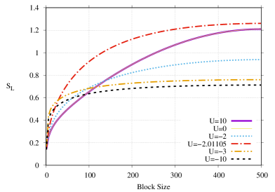
Figure 2: Block entropy vs block size in the ground state of Hamiltonian (1) with two fermions and $N=1001$. Curves for $U=0$ and $U=10$ appear superimposed, showing there is little change in the system’s response over the whole range of positive values of $U$. Block entropy saturates on every case, but a chain with maximum entanglement is observed for a negative value of $U$, indicating that a local interaction can have an enhancing effect on long-range entanglement when properly combined with hopping, even in the absence of phase transitions. In all cases shown $J=1$.

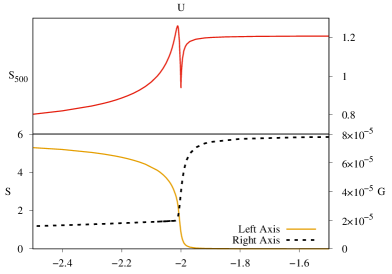
Figure 3: Top: Entanglement between the two halves of a chain describing the ground state of Hamiltonian (1) with two fermions and $N=1001$. A local minimum is observed at $U=-2$ and a global maximum at around $U=-2.011$. Bottom, left axis: Two-body entropy on the same system. Right axis: Energy gap. A sharp fluctuation in the block entanglement takes place around a short window of values of $U$ where the two-body entropy is halfway between zero and its saturation value, clearly indicating a correlation involving entanglement and the interplay between single- and many-bodyness. In all cases shown $J=1$.

Block entanglement as a function of block size is depicted in figure 2 for a Bethe chain with two fermions and $N=1001$. The dependency pattern is basically the same over the values of $U$ where two-body entropy, which can be seen in the bottom panel of figure 3, is small relative to its saturation value. Specifically, this occurs over the range of values of $U/J$ between $-1.9$ and infinity. Just under $-1.9$, the maximum value of block entropy displays a sharp fluctuation, as can be seen in the top panel of figure 3. A global maximum and a local minimum show up over a short window in the interaction domain. Furthermore, the gap remains finite throughout the parameter range, showing no phase transition, either conventional or topological, takes place. However, block entanglement displays a maximum at a point where the value of $S$ shows a clear contribution, yet not an overtaking, of many-bodyness. This suggests that it is not many-bodyness alone that causes entanglement to peak, but rather the interplay between single- and many-bodyness, since entanglement fluctuates at finite values of $U$ where neither interaction nor hopping is dominant. From a technical perspective, the interaction term alone has eigenstates that span over the local sector of the Fock basis, while the hopping term alone displays eigenstates that span on the single-body sector of the spectrum. It is therefore only when the Hamiltonian parameters stand in a range where both interaction and hopping prevail that the superposition distribution spreads over a wider sector of the Hilbert space and entanglement develops. The fact that this can happen even in the absence of a phase transition suggests that the entanglement that spontaneously arises in physical systems is more dependent on the level of access to the elements of a basis than it might be on criticality itself. In this sense, the half-filled chain has the maximum entanglement potential.

V Discussion

Interestingly, there is another way of writing $|E_{R}\rangle$ in (42) as a MPS. For this, let us see that over this state one can apply the next unitary transformation

$$\hat{M}_{1}=e^{i\phi_{1}\hat{m}_{1}}\text{, }\hat{m}_{1}=\frac{1}{2i}(|\omega_{2}\rangle\langle\omega_{1}|-|\omega_{1}\rangle\langle\omega_{2}|),$$ (54)

where

$$|\omega_{1}\rangle=|1100...00\rangle\text{, }|\omega_{2}\rangle=|001100...00\rangle.$$ (55)

The result being

$$\hat{M}_{1}|E_{R}\rangle=\left(\alpha_{1}\cos\frac{\phi_{1}}{2}-\alpha_{2}\sin\frac{\phi_{1}}{2}\right)|\omega_{1}\rangle$$

$$+\left(\alpha_{2}\cos\frac{\phi_{1}}{2}+\alpha_{1}\sin\frac{\phi_{1}}{2}\right)|\omega_{2}\rangle+\alpha_{3}|\omega_{3}\rangle...,$$ (56)

with $|\omega_{3}\rangle$ having a meaning equivalent to that of $|\omega_{1}\rangle$ and $|\omega_{2}\rangle$ in (55). The coefficient of $|\omega_{1}\rangle$ can always be made to vanish by choosing:

$$\tan\frac{\phi_{1}}{2}=\frac{\alpha_{2}}{\alpha_{1}}.$$ (57)

In similarity to the folding protocol described in section II, an analogous transformation can be applied to this reduced state, this time involving $|\omega_{2}\rangle$ and $|\omega_{3}\rangle$ in order to eliminate $|\omega_{2}\rangle$. The process continues until one last Fock state remains. The original state can then be obtained by reversing the procedure:

$$|E_{R}\rangle=\prod_{l}\hat{M}_{l}^{-1}|00...011\rangle.$$ (58)

Replacing this expression in (41) it is possible to express $|E\rangle$ as a series of unitary transformations applied on a simple Fock state easily expressible as MPS. In principle, this possibility offers another simulation path implementable by MPS. However, on closer inspection a potential complication arises: Transformations of the type $\hat{M}_{l}^{-1}$ in (58) are not like the $\hat{W}_{j,k}^{-1}$ in (41). The latter operate on next neighbors, while the former operate on sets of four nearest neighbors. This contrast with the fact that current MPS protocols are based on the repeated application of next-neighbor operations on tensor networks. This does not mean that the $\hat{M}_{l}^{-1}$s cannot be implemented over a tensor network, but such an implementation requires additional considerations. As a solution, one could think of establishing a local space of the original chain consisting not of one site but of two sites, so that a transformation involving four-nearest neighbors could be equivalently realized as a next-neighbor transformation. Contrariwise, when interaction is zero there is no need to consider four-nearest neighbor transformations because in that case two-body entropy vanishes and $|E_{R}\rangle$ is a Fock state, meaning that the decomposition depends entirely on genuine next-neighbor unitaries. This explains why methods based on MPS work so well on non-interacting systems. It also suggest a way of implementing variational MPS to find ground states of interacting systems: Instead of initializing the network as an uncorrelated state, the initial configuration should include many-body correlations in analogy to $|E_{R}\rangle$ in (42). In this way, the coefficients of this initial configuration become variational parameters, just as the elements of the tensor network, and should be determined as part of an energy-minimization algorithm. Another way of using tensor networks to find ground states is through imaginary-time evolution orus . This requires to split the evolution operator into a product of unitaries using a Suzuki-Trotter expansion suzuki . The approximation parameter is the time slice. The smaller the time slice the better the expansion accuracy. However, if the ground state does contain many-body correlations the following contradiction comes into play: Using small time slices is good to preserve the canonical representation and keep errors under control, but it is bad to approach the authentic ground state because such a state cannot be written in terms of a product of next-neighbor unitaries on an uncorrelated initial state. This is consistent with observations that the simulation accuracy peaks at relatively high values of the time slice and decreases as the time slice is shrunk reslen4 . The solution is then to incorporate many-body correlations on the initial state, although this add parameters that must be determined variationally, as before. This shows how important it is to establish a measurement of many-bodyness in systems with more than two fermions. Unfortunately, equation (52) is not scalable because there is no way of factorizing a tensor of more than two indices in a way analogous to (6), which is related to the fact that there is no way of effectuating higher order Schmidt decompositions peres . Even so, there might be other many-body criteria with equivalent functionality. Ground states displaying area laws do not necessarily have small many-body correlations. From figures 2 and 3 it can be seen that systems with very negative $U$ show rapid entanglement-saturation, but also high values of $S$. In spite of following area laws, these systems are most likely to present convergence issues when simulated via next-neighbor MPS-methods if many-body correlations are not incorporated on the initial state. This is the opposite of what happens for positive values of $U$, where the value of many-bodyness is notoriously marginal. Such a range circumscribes a set of highly interacting systems whose ground states can be effectively simulated using conventional tensor networks techniques.

VI Conclusions

The MPS structure of a two-fermion chain exactly solvable by Bethe ansatz has been analytically obtained and used to study the relation between entanglement and many-bodyness. Maximally entangled chains are observed when the state stands halfway between single- and many-bodyness. The study shows how to obtain any eigenstate as a product of unitary operators acting on an uncorrelated state. This decomposition reveals that states without many-body correlations can be written as a product of next-nearest-neighbor unitaries, whilst states with many-body correlations need four-nearest-neighbor unitaries in addition. This feature clashes with the assumption that the ground state of interacting Hamiltonians can be obtained as a sequence of next-neighbor operations, a premise that is fundamental in the formulation of many MPS methods. A potential solution is to incorporate many-body correlations on the initial state, but the quantification of such correlations in systems with more than two fermions needs characterization. Ultimately, block entanglement is not the only determining factor in MPS simulations, but also the amount of many-body correlations contained by the target state. Conventional MPS methods are better suited to systems where the ground state has little many-body entropy.

Appendix A Bethe Anzats

Let us consider a chain where two fermions can tunnel between adjacent places and interact when they simultaneously occupy neighboring sites of a chain with $N$ sites bethe . The system’s physics is described by the Hamiltonian

$$\hat{H}=\overbrace{J\sum_{j=1}^{N}(\hat{c}_{j}^{\dagger}\hat{c}_{j+1}+\hat{c}_{j+1}^{\dagger}\hat{c}_{j})}^{\hat{H}_{J}}+\overbrace{U\sum_{j=1}^{N}\hat{c}_{j+1}^{\dagger}\hat{c}_{j+1}\hat{c}_{j}^{\dagger}}^{\hat{H}_{U}}\hat{c}_{j}.$$ (59)

Mode operators satisfy standard fermionic rules $\{\hat{c}_{j},\hat{c}_{k}^{\dagger}\}=\delta_{j}^{k}$ and $\{\hat{c}_{j},\hat{c}_{k}\}=0$. Constants $J$ and $U$ determine the intensity of hopping and interaction respectively. The chain displays periodic boundary conditions, so that $\hat{c}_{j+N}=\hat{c}_{j}$. An eigenstate of a chain is hypothesized to be of the form

$$|E\rangle=[q_{1}\hat{\psi}(k_{1},k_{2})+q_{2}\hat{\psi}(k_{2},k_{1})]|0\rangle,$$ (60)

where

$$\hat{\psi}(k_{1},k_{2})=\sum_{m_{1}=1}^{N-1}\sum_{m_{2}=m_{1}+1}^{N}e^{ik_{1}m_{1}+ik_{2}m_{2}}\hat{c}_{m_{1}}^{\dagger}\hat{c}_{m_{2}}^{\dagger}.$$ (61)

Coefficients $q_{1}$, $q_{2}$, $k_{1}$ and $k_{2}$ are in general complex and must be adjusted to make $|E\rangle$ and eigenstate of $\hat{H}$. Ket $|0\rangle$ represents a state without fermions. In order to test the proposed solution, the effect of the hopping term is calculated, so obtaining the following expression

$$|\hat{H}_{J}E\rangle/J=2(\cos k_{1}+\cos k_{2})|E\rangle$$

$$-(q_{1}+q_{2})(1+e^{i(k_{1}+k_{2})})\sum_{m=1}^{N}e^{i(k_{1}+k_{2})m}\hat{c}_{m}^{\dagger}\hat{c}_{m+1}^{\dagger}|0\rangle$$

$$-(q_{1}+q_{2}e^{ik_{1}N})\sum_{m=1}^{N-1}e^{ik_{2}m}(\hat{c}_{1}^{\dagger}\hat{c}_{m}^{\dagger}+e^{ik_{1}}\hat{c}_{m}^{\dagger}\hat{c}_{N}^{\dagger})|0\rangle$$

$$-(q_{2}+q_{1}e^{ik_{2}N})\sum_{m=1}^{N-1}e^{ik_{1}m}(\hat{c}_{1}^{\dagger}\hat{c}_{m}^{\dagger}+e^{ik_{2}}\hat{c}_{m}^{\dagger}\hat{c}_{N}^{\dagger})|0\rangle.$$ (62)

When $k_{1}\neq k_{2}$ terms in the last two lines can be canceled by setting

$$q_{2}=-q_{1}e^{ik_{2}N}=-q_{1}e^{-ik_{1}N}$$ (63)

$$\rightarrow e^{i(k_{1}+k_{2})N}=1.$$ (64)

The latter requirement can be met through the following relation

$$k_{1}+k_{2}=\frac{2\pi n}{N},\text{ }n=0,1,...,N-1.$$ (65)

Regarding the interaction part of the Hamiltonian, it can be shown that

$$|\hat{H}_{U}E\rangle/U=(q_{1}e^{ik_{2}}+q_{2}e^{ik_{1}})\sum_{m=1}^{N}e^{i(k_{1}+k_{2})m}\hat{c}_{m}^{\dagger}\hat{c}_{m+1}^{\dagger}|0\rangle.$$ (66)

Both (63) and (64) have been utilized in the calculation leading to (66). Using the expressions obtained above for hopping and interaction the eigenvalue equation can be formulated as

$$|\hat{H}E\rangle=2J(\cos k_{1}+\cos k_{2})|E\rangle$$

$$+\left(U(q_{1}e^{ik_{2}}+q_{2}e^{ik_{1}})-J(q_{1}+q_{2})(1+e^{i(k_{1}+k_{2})})\right)$$

$$\times\sum_{m=1}^{N}e^{i(k_{1}+k_{2})m}\hat{c}_{m}^{\dagger}\hat{c}_{m+1}^{\dagger}|0\rangle.$$ (67)

Using again equations (63) and (64) it can be shown that the term in parentheses vanishes for values of $z=e^{-ik_{1}}$ being solutions of

$$(1+\alpha_{n})z^{N}-\gamma z^{N-1}+\gamma\alpha_{n}z-(1+\alpha_{n})=0,$$ (68)

where

$$\alpha_{n}=e^{i\frac{2\pi n}{N}},\text{ }n=0,1,...,N-1,\text{ and }\gamma=\frac{U}{J},\text{ }J\neq 0.$$ (69)

Notice that if $\alpha_{n}=-1$, which can happen only when $N$ is even, the order of polynomial (68) is reduced. Once $k_{1}$ has been determined from $z$, $k_{2}$ can be found from (65). These constants can be used to find the system energy from

$$E=2J(\cos k_{1}+\cos k_{2}).$$ (70)

Constants $q_{1}$ and $q_{2}$ can be determined using equation (63) and the normalization condition for eigenstates. From the whole set of solutions that can be built in this way, some might be redundant. This happens because swapping $k_{1}\leftrightarrow k_{2}$ does not change state (60), as can be implied from the next identity (derived using (63) and (64))

$$q_{1}\hat{\psi}(k_{2},k_{1})+q_{2}\hat{\psi}(k_{1},k_{2})$$

$$=-e^{ik_{1}N}(q_{1}\hat{\psi}(k_{1},k_{2})+q_{2}\hat{\psi}(k_{2},k_{1})).$$ (71)

Hence, one can discard a pair $(k_{1}^{\prime},k_{2}^{\prime})$ whose relation to another complying pair $(k_{1},k_{2})$ be $(k_{1}^{\prime},k_{2}^{\prime})=(k_{2},k_{1})$. It can happen that some solutions provided by (68) derive in complex $k$s. Such solutions are valid. Moreover, in this case $k_{1}=k_{2}^{*}$ in order for relations (64) and (70) to hold. The following particular cases must be analysed separately

1. $\alpha_{n}=-1$ and $\gamma\neq 0$ For this $n=\frac{N}{2}$ and therefore $N$ must be even. Equation (68) is then reduced to

   $$z^{N-2}+1=0.$$ (72)

   Technically, $z=0$ is also a root but it does not lead to any meaningful solution. From (72) it follows

   $$z=e^{i\pi(2j+1)/(N-2)},\text{ }j=0,1,...,N-3.$$ (73)

   The rest of parameters can be found from $z$ according to the procedure prescribed above.

2. $\gamma=0$ $(U=0,J\neq 0)$. An inspection of the solutions provided by equation (68) in this regime evidences a number of inconsistencies, in particular, some solutions are not independent. In this case it is better to build independet solutions using a different protocol. This can be done without major complications by observing that in absence of interaction a solution can be written as

   $$|E\rangle=\sum_{m_{1}=1}^{N}e^{ik_{1}m_{1}}\hat{c}_{m_{1}}^{\dagger}\sum_{m_{2}=1}^{N}e^{ik_{2}m_{2}}\hat{c}_{m_{2}}^{\dagger}|0\rangle.$$ (74)

   This form is a particular case of the Bethe solution in (60) when $q_{2}=-q_{1}$. In order to guarantee orthogonal solutions, $k_{1}$ and $k_{2}$ must take the next form

   $$k_{1}=2\pi j_{1}/N,\text{ }k_{2}=2\pi j_{2}/N.$$ (75)

   Both $j_{1}$ and $j_{2}$ are integers that can take values between 1 and $N$ under the constrain $j_{1}<j_{2}$. The corresponding energy can be obtained through equation (70) replacing $k_{1}$ and $k_{2}$. The solutions obtained in this way are independent and form a complete set.

3. It happens that after solving equation (68) and finding the constants of interest, some solutions with $k_{1}=k_{2}=k$ turn up. The significance of such solutions must be inspected. In this case the procedure followed to arrive at (68) is compromised because the terms in the last two lines of equation (62) group in a different way, namely

   $$(q_{1}+q_{2})(1+e^{ikN})\sum_{m=1}^{N-1}e^{ikm}(\hat{c}_{1}^{\dagger}\hat{c}_{m}^{\dagger}+e^{ik}\hat{c}_{m}^{\dagger}\hat{c}_{N}^{\dagger})|0\rangle.$$ (76)

   In principle, it appears there are two ways of cancelling this contribution. In the first place, one can set

   $$k=\frac{\pi(2j+1)}{N},\text{ }j=0,1,...$$ (77)

   This is the same estimation of $k$ that can be obtained through (65) by setting $k_{1}=k_{2}=k$ and selecting $n$ odd. However, relation (63) is no longer required to complete the cancellation. Since such a relation has been used to get (68), expression (68) itself losses validity and any solution provided by it that might display equal $k$s is unreliable. One can however group terms and prove that the term in parenthesis in equation (67) takes the next form

   $$(q_{1}+q_{2})(Ue^{ik}-J(1+e^{2ik}))=0.$$ (78)

   Because at this stage $k$ is already given by (77), the only possibility is to make $q_{2}=-q_{1}$, which is in contradiction with equation (63) for the values of $k$ taken in (77), making it clear that in this case equation (68) is flawed. Hence it follows making $q_{1}=-q_{2}$ is the only way the whole term (76) can be canceled. Just as in the previous case, equation (63) is not enforced and therefore the solutions provided by (68) cannot be admitted. Constant $k$ is no longer conditioned by (77). However, making $k_{1}=k_{2}$ and $q_{2}=-q_{1}$ at the same time identically nullifies the original anzats in (60). Thus, there cannot be relevant solutions with equal $k$s and therefore any solution arising from the protocol displaying such a feature is discarded.

4. There is one solution that eludes the anzats. Let us consider an eigenstate with the following structure

   $$|E\rangle=q\sum_{m=1}^{N}e^{ikm}\hat{c}_{m}^{\dagger}\hat{c}_{m+1}^{\dagger}|0\rangle.$$ (79)

   Constant $q$ is essentially a normalization parameter. The effect of the hopping term on this state can be written as

   $$|\hat{H}_{J}E\rangle/qJ=(1+e^{ik})\sum_{m=1}^{N}e^{ikj}\hat{c}_{j}^{\dagger}\hat{c}_{j+2}^{\dagger}|0\rangle$$

   $$+(1-e^{ikN})\hat{c}_{N}^{\dagger}\hat{c}_{2}^{\dagger}|0\rangle.$$ (80)

   The whole term can be nullified by making $k=\pi$, but only if $N$ is even. Since state (79) is in general an eigenstate of $\hat{H}_{U}$, in this specific case it becomes an eigenstate of $\hat{H}$ too. Constant $J$ makes no contribution to energy and the corresponding eigenvalue equation becomes

   $$|\hat{H}E\rangle=U|E\rangle.$$ (81)

   This single solution that arises when $N$ is even and $U\neq 0$ must be added to the eigenstates obtained using the Bethe anzats to form a complete set of solutions.

Taking this considerations into account, the total number of independent solutions turns out to be $N(N-1)/2$, regardless of the parity of $N$. This is the correct number of solutions in a system where two fermions can access $N$ single-body states.

References

- (1) J. Cirac, D. Pérez-García, N. Schuch and F. Verstraetea Matrix product states and projected entangled pair states: Concepts, symmetries, theorems Review of Modern Physics 93 045003 (2021).
- (2) S.R. White, Physical Review Letters Density matrix formulation for quantum renormalization groups 69 2863 (1992).
- (3) G. Vidal, Physical Review Letters Efficient simulation of one-dimensional quantum many body systems 93 040502 (2004).
- (4) U. Schollwock, Annals of Physics The density-matrix renormalization group in the age of matrix product states 326 96 (2011).
- (5) M. Ganahl et. al. arXiv:2204.05693.
- (6) A. Polkovnikov, K. Sengupta, A. Silva and M. Vengalattore Colloquium: Nonequilibrium dynamics of closed interacting quantum systems Reviews of Modern Physics 83 863 (2011).
- (7) G. Vidal, J. Latorre, E. Rico and A. Kitaev Entanglement in Quantum Critical Phenomena Physical Review Letters 90 227902 (2003).
- (8) J. Eisert, M. Cramer and M. Plenio Colloquium: Area laws for the entanglement entropy Reviews of Modern Physics 82 277 (2010).
- (9) L. Amico, R. Fazio, A. Osterloh and V. Vedral Entanglement in many body systems Review of Modern Physics 80 517 (2008).
- (10) G. Casati, I. Guarneri and J. Reslen Classical dynamics of quantum entanglement Physical Review E 85 036208 (2012).
- (11) A. Lerose and S. Pappalardi Bridging entanglement dynamics and chaos in semiclassical systems Physical Review A 102 032404 (2020).
- (12) H. Bethe Zur Theorie der Metalle Zeitschrift für Physik 71 205 (1931). Translation by T. Dorlas (2009).
- (13) J. Van Dyke, G. Barron, N. Mayhall, E. Barnes and S. Economoua Preparing Bethe Ansatz Eigenstates on a Quantum Computer PRX Quantum 2 040329 (2021).
- (14) H. Barghathi, E. Casiano-Diaz and A. Del Maestro Particle partition entanglement of one dimensional spinless fermions Journal of Statistical Mechanics: Theory and Experiment 083108 (2017).
- (15) H. Barghathi, E. Casiano-Diaz, and A. Del Maestro Operationally accessible entanglement of one-dimensional spinless fermions Physical Review A 100 022324 (2019).
- (16) E. Casiano-Diaz Quantum entanglement of one-dimensional spinless fermions Graduate College Dissertations and Theses. 1052. (2019).
- (17) D. Youla A normal form for a matrix under the unitary congruence group Canadian Journal of Mathematics 13 694 (1961).
- (18) J. Reslen End-to-end correlations in the Kitaev chain Journal of Physics Communications 2 105006 (2018).
- (19) J. Reslen Uncoupled Majorana fermions in open quantum systems: on the efficient simulation of non-equilibrium stationary states of quadratic Fermi models Journal of Physics: Condensed Matter 32 405601 (2020).
- (20) J. Reslen Operator folding and matrix product states in linearly-coupled bosonic arrays Mexican Journal of Physics (RMF) 59 482 (2013).
- (21) J. Reslen Mode folding in systems with local interaction: unitary and non-unitary transformations using tensor states Journal of Physics A: Mathematical and Theoretical 48 175301 (2015).
- (22) G. Vidal Efficient classical simulation of slightly entangled quantum computations Physical Review Letters 91:147901, 2003.
- (23) C. Bennett, H. Bernstein, S. Popescu and B. Schumache Concentrating partial entanglement by local operations Physical Review A 53 2046 (1996).
- (24) R. Orus and G. Vidal Infinite time-evolving block decimation algorithm beyond unitary evolution Physical Review B 78 155117 (2008).
- (25) M. Suzuki Decomposition formulas of exponential operators and Lie exponentials with some applications to quantum mechanics and statistical physics Journal of Mathematical Physics 26 601 (1985).
- (26) A. Peres Higher order Schmidt decompositions Physics Letters A 202:16 (1995).