On non-centered maximal operators related to
a non-doubling and non-radial exponential measure

Abstract.

We investigate mapping properties of non-centered Hardy-Littlewood maximal operators related to the exponential measure $d\mu(x)=\exp(-|x_{1}|-\ldots-|x_{d}|)dx$ in $\mathbb{R}^{d}$. The mean values are taken over Euclidean balls or cubes ($\ell^{\infty}$ balls) or diamonds ($\ell^{1}$ balls). Assuming that $d\geq 2$, in the cases of cubes and diamonds we prove the $L^{p}$-boundedness for $p>1$ and disprove the weak type $(1,1)$ estimate. The same is proved in the case of Euclidean balls, under the restriction $d\leq 4$ for the positive part.

1. Introduction and statement of the results

Let $d\geq 1$. Consider a metric measure space $(\mathbb{R}^{d},\rho,d\eta)$, with a Borel measure $\eta$ which is non-negative, non-trivial and locally finite. The associated non-centered Hardy-Littlewood maximal operator is defined by

$$M_{\eta}f(x)=\sup_{B_{\rho}\ni x}\frac{1}{\eta(B_{\rho})}\int_{B_{\rho}}|f|\,d\eta,\qquad x\in\mathbb{R}^{d},$$

where the supremum is taken over all open metric balls related to $\rho$ that contain $x$ and have strictly positive measure $\eta$. Here $f$ is any Borel measurable function on $\mathbb{R}^{d}$. The centered variant of $M_{\eta}$, denoted by $M_{\eta}^{c}$, arises by restricting the supremum to balls centered at $x$. Clearly, $M_{\eta}^{c}f\leq M_{\eta}f$. Furthermore, $M_{\eta}$ is trivially bounded on $L^{\infty}$.

When $\eta$ is doubling, the two maximal operators are comparable and satisfy the weak type $(1,1)$ estimate with respect to $\eta$. The latter follows from a Vitali type covering lemma, cf. [4, Chapter 2]. Then, by interpolation, $M_{\eta}$ and $M_{\eta}^{c}$ are bounded on $L^{p}(d\eta)$ for $p>1$.

It is also well known, at least for the Euclidean distance $\rho$, that (see e.g. [2, p. 44]) whatever the measure $\eta$ is, $M_{\eta}^{c}$ is always of weak type $(1,1)$ with respect to $\eta$, thus also bounded on $L^{p}(d\eta)$ for $p>1$. The former is a consequence of the Besicovitch-Morse covering lemma. In dimension one the larger uncentered operator $M_{\eta}$ behaves in the same way (see [2, p. 45]), that is, it is of weak type $(1,1)$ and bounded on $L^{p}(d\eta)$, $p>1$, independently of the doubling property of $\eta$. However, this is no longer true in general in higher dimensions.

One of the authors [15] proved that for $d=2$ (implicitly $d\geq 2$) and either the Euclidean or the $\ell^{\infty}$ distance $\rho$, and the Gaussian measure $\eta$, the weak type $(1,1)$ estimate for $M_{\eta}$ fails. Nevertheless, as shown by Forzani et al. [3], the $L^{p}$-boundedness for $p>1$ in this case still holds, though the convenient interpolation argument is inapplicable. Similar results for certain classes of rotationally invariant measures $\eta$ were established in [6, 14, 16, 17], among others. It is interesting to point out that there are radial measures $\eta$ for which $M_{\eta}$ is not even weak type $(p,p)$ for any $p<\infty$, see [5, 6, 17].

It should be mentioned that so far non-centered Hardy-Littlewood maximal operators for non-doubling measures were studied in various settings and spaces also different from $\mathbb{R}^{d}$, for example in the framework of cusped manifolds [8, 9].

The main aim of this paper is to study the maximal operator $M_{\eta}$ when the distance $\rho$ is the Euclidean one and for the particular exponential measure $\eta=\mu$,

$$d\mu(x)=\exp\big{(}-|x_{1}|-\ldots-|x_{d}|\big{)}\,dx.$$

Our motivation is to provide both methods and results in this model case where the measure is non-doubling and non-radial, since the literature seems to lack a basic example of this kind. Only recently H.-Q. Li, Y. Wu and one of the authors [10] considered $M_{\eta}$ essentially for $d\eta(x)=e^{x_{1}}dx$ in $\mathbb{R}^{d}$. In this case the measure, in contrast with $\mu$, is neither finite nor even in each variable. Moreover, it has a simple structure that makes the associated analysis relatively straightforward.

The measure $\mu$ is not radial in the sense of the Euclidean distance, nevertheless it is radial with respect to the $\ell^{1}$ metric. Thus one might wonder whether, perhaps, the maximal operator behaves better when $\rho$ is the seemingly better matching $\ell^{1}$ distance. This issue led us to study $M_{\mu}$ also when $\rho$ is the $\ell^{1}$ metric, as well as in the opposite extreme case where $\rho$ is the $\ell^{\infty}$ metric.

Denote by $M_{\mu}^{\mathcal{B}}$, $M_{\mu}^{\mathcal{Q}}$, $M_{\mu}^{\mathcal{D}}$ the maximal operators $M_{\mu}$ with the underlying $\ell^{2}$ or $\ell^{\infty}$ or $\ell^{1}$ metric, respectively. Note that the metric balls in the first case are just the Euclidean balls $\mathcal{B}$, and in the second case the Euclidean cubes $\mathcal{Q}$ with sides parallel to the coordinate axes. The third case is geometrically somewhat more complicated, and we call the metric balls diamonds $\mathcal{D}$ in this situation. Notice that in dimension $d=2$ the diamonds are simply rotated cubes (or actually squares), but there is no similar relation in higher dimensions.

Our main result is the following theorem. We strongly believe it will be an inspiration for considering $M_{\eta}$ with more general non-radial and non-doubling $\eta$, and for further research in the future.

Theorem 1.

Let $d\geq 2$.

• None of the maximal operators $M_{\mu}^{\mathcal{B}}$, $M_{\mu}^{\mathcal{Q}}$, $M_{\mu}^{\mathcal{D}}$ is of weak type $(1,1)$.

• The operators $M_{\mu}^{\mathcal{Q}}$ and $M_{\mu}^{\mathcal{D}}$ are bounded on $L^{p}(d\mu)$ for $p>1$. The same is true for $M_{\mu}^{\mathcal{B}}$, provided that $d\leq 4$.

Remark 1.1.

The restriction $d\leq 4$ in Theorem 1(B), the case of $M_{\mu}^{\mathcal{B}}$, is caused by substantial technical difficulties of geometrical nature in proving the result in dimensions $d=5$ and higher. Nevertheless, we strongly believe that the result is true for any $d\geq 2$.

When $d=1$, in view of what was said above, all the three maximal operators coincide and are of weak type $(1,1)$ and bounded on $L^{p}(d\mu)$, $p>1$. Note that the latter readily implies Theorem 1(B) for $M_{\mu}^{\mathcal{Q}}$. Indeed, due to the product structure of the cubes $M_{\mu}^{\mathcal{Q}}$ can be controlled by a composition of the one-dimensional operators.

Theorem 1 reveals that the $L^{p}$ behavior of $M_{\mu}^{\mathcal{B}}$ and $M_{\mu}^{\mathcal{Q}}$ is exactly the same as in case of their counterparts for the Gaussian measure [15, 3]. In particular, we see that the local doubling property (see Section 2), satisfied by $\mu$ but not by the Gaussian measure, does not lead here to any improvement.

An interesting but technically quite complicated problem is to generalize Theorem 1 to Laguerre-type measures of the form

(1.1) $$d\mu_{\alpha}(x)=\prod_{i=1}^{d}|x_{i}|^{\alpha_{i}}\exp\big{(}-|x_{i}|\big{)}\,dx,$$

where $\alpha=(\alpha_{1},\ldots,\alpha_{d})\in(-1,\infty)^{d}$ is a fixed multi-parameter. Clearly, the special choice $\alpha=(0,\ldots,0)$ gives $\mu$. The restriction of the measure space $(\mathbb{R}^{d},d\mu_{\alpha})$ to $(0,\infty)^{d}$ forms a natural environment for analysis related to the classical Laguerre operator. Analysis of various objects in this context has already received considerable attention; see for instance [1, 11, 12, 13] and references given there. Thus any knowledge about the non-centered Hardy-Littlewood maximal operator $M_{\mu_{\alpha}}$ or its variants would be potentially useful. For some negative results, see Remark 3.1 below, which says that $M_{\mu_{\alpha}}$ is not of weak type $(1,1)$ when the underlying metric is either $\ell^{2}$ or $\ell^{\infty}$.

The remaining part of the paper is devoted to the proof of Theorem 1. The subsequent sections contain technical preliminaries, the proof of Theorem 1(A) and the proof of Theorem 1(B), respectively.

2. Technical preliminaries

Denote $\mathbb{R}^{d}_{+}=(0,\infty)^{d}$, $d\geq 1$. For brevity the restriction of $\mu$ to $\mathbb{R}^{d}_{+}$ will be denoted by the same symbol. We write $|\cdot|_{q}$ for the $\ell^{q}$, $1\leq q\leq\infty$, norm in $\mathbb{R}^{d}$,

$$|x|_{q}=\bigg{(}\sum_{i=1}^{d}|x_{i}|^{q}\bigg{)}^{1/q}\quad\textrm{if}\quad q<\infty,\qquad|x|_{\infty}=\max_{1\leq i\leq d}|x_{i}|.$$

Of course, this norm generates a metric $\rho_{q}$ both in $\mathbb{R}^{d}$ and $\mathbb{R}^{d}_{+}$. For $q=1,2,\infty$ we denote the families of open balls in the metric measure spaces $(\mathbb{R}^{d}_{+},\rho_{q},d\mu)$ by $\mathcal{D}_{+}$, $\mathcal{B}_{+}$, $\mathcal{Q}_{+}$, respectively. Notice that these are exactly diamonds, Euclidean balls and cubes, respectively, centered in and intersected with $\mathbb{R}^{d}_{+}$.

Bring in the non-centered Hardy-Littlewood maximal operator

$$M_{\mu}^{\mathcal{B}_{+}}f(x)=\sup_{x\in B\in\mathcal{B}_{+}}\frac{1}{\mu(B)}\int_{B}|f|\,d\mu,\qquad x\in\mathbb{R}^{d}_{+},$$

and analogously $M_{\mu}^{\mathcal{Q}_{+}}$ and $M_{\mu}^{\mathcal{D}_{+}}$. The following elementary result shows that proving Theorem 1 can be reduced to a similar analysis for $M_{\mu}^{\mathcal{B}_{+}}$, $M_{\mu}^{\mathcal{Q}_{+}}$ and $M_{\mu}^{\mathcal{D}_{+}}$.

Proposition 2.1.

Let $d\geq 1$ and $p>1$ be fixed. The operator $M_{\mu}^{\mathcal{B}}$ is bounded on $L^{p}(\mathbb{R}^{d},d\mu)$ (is weak type $(1,1)$ with respect to $(\mathbb{R}^{d},d\mu)$) if and only if $M_{\mu}^{\mathcal{B}_{+}}$ is bounded on $L^{p}(\mathbb{R}^{d}_{+},d\mu)$ (is weak type $(1,1)$ with respect to $(\mathbb{R}^{d}_{+},d\mu)$).

The same relations hold between $M_{\mu}^{\mathcal{Q}}$ and $M_{\mu}^{\mathcal{Q}_{+}}$, as well as between $M_{\mu}^{\mathcal{D}}$ and $M_{\mu}^{\mathcal{D}_{+}}$.

Proof.

This is a consequence of the symmetries involved. Use either the even (more precisely even with respect to each coordinate axis) extension to $\mathbb{R}^{d}$ of $f_{+}$ on $\mathbb{R}^{d}_{+}$ or, for the other implication, the decomposition of $f$ on $\mathbb{R}^{d}$ into its symmetric components which are either even or odd with respect to each coordinate axis. ∎

Thus, from now on, we focus on the restricted operators $M_{\mu}^{\mathcal{B}_{+}}$, $M_{\mu}^{\mathcal{Q}_{+}}$ and $M_{\mu}^{\mathcal{D}_{+}}$. This is a crucial reduction from a technical point of view, since in $\mathbb{R}_{+}^{d}$ the measure $\mu$ has a simpler analytic structure than in $\mathbb{R}^{d}$ (no absolute values involved). From now on $\mu$ will denote the restriction of the measure with density $\exp(-|x|_{1})$ to $\mathbb{R}^{d}_{+}$.

In what follows we shall write $X\lesssim Y$ with $Y>0$ to indicate that $X\leq CY$ with a constant $C>0$ depending only on the dimension and on $p$ in the proofs of $L^{p}$ estimates, and also on $\alpha$ in Remarks 2.4 and 3.1. We write $X\simeq Y$ when simultaneously $X\lesssim Y$ and $Y\lesssim X$.

We will occasionally refer to the strong maximal operator in Euclidean space with Lebesgue measure. It is defined as

(2.1) $$M_{\mathrm{str}}f(x)=\sup\frac{1}{|R|}\,\int_{R}|f(y)|\,dy,$$

where the supremum is taken over all rectangles with edges parallel with the coordinate axes and containing $x$. It is well known that $M_{\mathrm{str}}$ is bounded on $L^{p}(dx)$ for $1<p\leq\infty$, as seen by iterating the one-dimensional estimate.

We shall use the following notation for $\ell^{1}$, $\ell^{2}$ and $\ell^{\infty}$ balls in $\mathbb{R}^{d}_{+}$. For $x\in\mathbb{R}^{d}_{+}$ and $r>0$

$$D(x,r) =\big{\{}y\in\mathbb{R}^{d}_{+}:|x-y|_{1}<r\big{\}},$$

$$B(x,r) =\big{\{}y\in\mathbb{R}^{d}_{+}:|x-y|_{2}<r\big{\}},$$

$$Q(x,r) =\big{\{}y\in\mathbb{R}^{d}_{+}:|x-y|_{\infty}<r\big{\}}.$$

Euclidean balls in all of $\mathbb{R}^{d}$ will be written as

$$\mathbf{B}(x,r)=\big{\{}y\in\mathbb{R}^{d}:|x-y|_{2}<r\big{\}}.$$

Further, we denote

$$\mathbf{1} =(1,\ldots,1)\in\mathbb{R}^{d}_{+},$$

$$\Sigma^{d-1}_{+} =\big{\{}x\in\mathbb{R}^{d}_{+}:|x|_{1}=1\big{\}},$$

$$a\vee b =\max(a,b),$$

$$a\wedge b =\min(a,b).$$

The measure $\mu$ is not doubling in $(\mathbb{R}^{d}_{+},\rho_{q},d\mu)$, $q=1,2,\infty$; nevertheless it is locally doubling in the following sense.

Lemma 2.2.

Let $d\geq 1$. Given $R>0$, there exists a constant $C_{R}>0$ such that

(2.2) $$\mu\big{(}Q(x,2r)\big{)}\leq C_{R}\;\mu\big{(}Q(x,r)\big{)},\qquad x\in\mathbb{R}^{d}_{+},\quad 0<r\leq R.$$

The same holds if $Q$ above is replaced either by $B$ or by $D$.

Proof.

This is elementary, since in any of the balls considered the density of $\mu$ varies at most by a factor depending only on $R$. ∎

Let $d\geq 1$. We now give sharp estimates for the measure of large cubes, balls and diamonds provided that they are disjoint with the boundary of $\mathbb{R}^{d}_{+}$. Consider a ball in one of the three metrics $\ell^{\infty},\>\ell^{2},\>\ell^{1}$ with center $x\in\mathbb{R}^{d}_{+}$ and radius $r$ satisfying $1\leq r\leq\min_{1\leq i\leq d}x_{i}$. We select a point $z_{q}=z_{q}(x,r)$ in the closure of this ball where $|\cdot|_{1}$ is minimal, i.e., the density of $\mu$ is maximal, as follows:

$$z_{\infty} =z_{\infty}(x,r)=x-r\,\mathbf{1},$$

$$z_{2} =z_{2}(x,r)=x-\frac{r}{\sqrt{d}}\,\mathbf{1},$$

$$z_{1} =z_{1}(x,r)=x-\frac{r}{d}\,\mathbf{1}.$$

Notice that $z_{\infty}$ and $z_{2}$ are unique points with this minimizing property, but $z_{1}$ is not.

Lemma 2.3.

Let $x\in\mathbb{R}^{d}_{+}$ and $1\leq r\leq x_{i},\>i=1,\dots,d$. Then the balls $Q(x,r)$, $B(x,r)$ and $D(x,r)$ are contained in $\mathbb{R}^{d}_{+}$ and

$$\mu\big{(}Q(x,r)\big{)} \simeq\exp(-|z_{\infty}|_{1}),$$

$$\mu\big{(}B(x,r)\big{)} \simeq\exp(-|z_{2}|_{1})\,r^{(d-1)/2},$$

$$\mu\big{(}D(x,r)\big{)} \simeq\exp(-|z_{1}|_{1})\,r^{d-1}.$$

The implicit constants here depend only on $d$.

Proof.

The inclusions follow, since if $y$ is in one of the balls, then $|y_{i}-x_{i}|<r$ for each $i$, so that $y_{i}>0$.

The estimate for cubes is straightforward. One has

$$\mu\big{(}Q(x,r)\big{)} =\int_{Q(x,r)}\exp(-|y|_{1})\,dy=\prod_{i=1}^{d}\Big{(}e^{-(x_{i}-r)}-e^{-(x_{i}+r)}\Big{)}$$

$$\simeq\exp(-|x|_{1})e^{rd}=\exp(-|z_{\infty}|_{1}).$$

To deal with the case of Euclidean balls, observe that any point in $B(x,r)$ can be written as $z_{2}+\frac{s}{\sqrt{d}}\,\mathbf{1}+y$, where $s>0$ and $y\perp\mathbf{1}$. Using the expression for $z_{2}$, we see that this point is in $B(x,r)$ precisely when $(r-s)^{2}+|y|^{2}<r^{2}$ or equivalently $|y|<\sqrt{2rs-s^{2}}$ and $0<s<2r$. We now integrate in $y$ in a hyperplane orthogonal to $\mathbf{1}$ and then in $s$, taking the density of $\mu$ into account. For the upper estimate, we simply write

$$\mu\big{(}B(x,r)\big{)} \lesssim\int_{0}^{2r}\exp\big{(}-|z_{2}|_{1}-\sqrt{d}\,s\big{)}\,(2rs-s^{2})^{(d-1)/2}\,ds$$

$$\lesssim\exp(-|z_{2}|_{1})\,\int_{0}^{\infty}\exp\big{(}-\sqrt{d}\,s\big{)}\,(rs)^{(d-1)/2}\,ds\simeq\exp(-|z_{2}|_{1})\,r^{(d-1)/2}.$$

To obtain the lower estimate, we observe that $2rs-s^{2}>rs$ for $0<s<r$ and argue similarly. Since $r\geq 1$, we get

$$\mu\big{(}B(x,r)\big{)}\gtrsim\int_{0}^{r}\exp\big{(}-|z_{2}|_{1}-\sqrt{d}\,s\big{)}\,(rs)^{(d-1)/2}\,ds\simeq\exp(-|z_{2}|_{1})\,r^{(d-1)/2}.$$

As for the diamonds, note that $|z_{1}|_{1}=|x|_{1}-r$. For $s>0$ the diameter of the intersection of ${D(x,r)}$ with the hyperplane $\{y:|y|_{1}=|x|_{1}-r+s\}$ is $\mathcal{O}(r)$. Integrating as before, we obtain the upper estimate.

On the other hand, consider the following set

$$\left\{x-\frac{r}{d}\,\mathbf{1}+\frac{s}{d}\,\mathbf{1}+y:\;0<s<r/2,\;\;y\perp\mathbf{1},\;\;|y_{i}|<\frac{r}{2d}\;\;\mathrm{for}\;\;i=1,\dots,d\right\}.$$

The $\ell^{1}$ distance from $x$ to a point in this set is

$$\sum_{i=1}^{d}\left|-\frac{r}{d}+\frac{s}{d}+y_{i}\right|=\sum_{i=1}^{d}\left(\frac{r}{d}-\frac{s}{d}-y_{i}\right)\leq{r-s}<r.$$

Thus ${D(x,r)}$ contains the set, and the lower estimate follows by integration. ∎

Remark 2.4.

Lemmas 2.2 and 2.3 can be generalized to the space $(\mathbb{R}^{d}_{+},\rho_{q},d\mu_{\alpha})$, where $q\in\{1,2,\infty\}$ and $\mu_{\alpha}$ is the restriction of the measure defined in (1.1). This means that $\mu_{\alpha}$ is locally doubling (but not doubling) in the context of this space. Moreover,

$$\mu_{\alpha}\big{(}E_{q}(x,r)\big{)}\simeq x_{1}^{\alpha_{1}}\cdot\ldots\cdot x_{d}^{\alpha_{d}}\exp(-|x|_{1})\,r^{(d-1)/q}e^{rd^{1-1/q}}$$

uniformly in $x\in\mathbb{R}^{d}_{+}$ and $1\leq r\leq\min_{1\leq i\leq d}x_{i}$; here $E_{q}(x,r)$ is the open ball in $(\mathbb{R}^{d}_{+},\rho_{q})$ centered at $x$ and of radius $r$.

Proposition 2.1 can also be generalized in a similar spirit.

We now pass to the proof of Theorem 1. It is worth indicating that the radiality of $\mu$ with respect to the $\ell^{1}$ norm will be heavily exploited, often implicitly, throughout our reasonings.

3. Proof of Theorem 1(A)

In this section we prove Theorem 1(A) working with the operators restricted to $\mathbb{R}^{d}_{+}$, see Proposition 2.1. The cases of $M_{\mu}^{\mathcal{Q}_{+}}$ and $M_{\mu}^{\mathcal{B}_{+}}$ will be treated together, since the argument is essentially the same. This argument has the advantage that it can be rather easily generalized to cover $M_{\mu_{\alpha}}^{\mathcal{Q}_{+}}$ and $M_{\mu_{\alpha}}^{\mathcal{B}_{+}}$ (analogues of $M_{\mu}^{\mathcal{Q}_{+}}$ and $M_{\mu}^{\mathcal{B}_{+}}$ for the measure $\mu_{\alpha}$), see Remark 3.1 below. Unfortunately, this argument does not apply to $M_{\mu}^{\mathcal{D}_{+}}$ since it uses essentially the non-radiality of the measure with respect to the norm. Therefore, we give a different argument for $M_{\mu}^{\mathcal{D}_{+}}$, but the question of its generalization to $M_{\mu_{\alpha}}^{\mathcal{D}_{+}}$ seems to be technically difficult and remains open.

Proof of Theorem 1(A), the cases of $\mathbf{M_{\mu}^{\mathcal{Q}}}$ and $\mathbf{M_{\mu}^{\mathcal{B}}}$

We first consider the case $d=2$ and then indicate the changes needed for $d\geq 3$. We begin with the operator $M_{\mu}^{\mathcal{Q}_{+}}$. Let $Q_{s}$, $s\geq 1$, denote the square centered at $(s,s)$ and of ‘radius’ $s/2$. Further, let $\widehat{Q_{s}}$ be the union of all squares obtained by moving $Q_{s}$ (or rather its center) along the line segment $\Delta_{s}$ which is the intersection of $\frac{1}{2}Q_{s}$ with the line $x+y=2s$, see Figure 1.

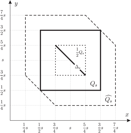
Figure 1. Counterexample for $M_{\mu}^{\mathcal{Q}_{+}}$ in dimension $d=2$.

Assuming a contrario that $M_{\mu}^{\mathcal{Q}_{+}}$ is of weak type $(1,1)$, we claim that

(3.1) $$\mu(\widehat{Q_{s}})\lesssim\mu(Q_{s}),\qquad s\geq 2.$$

To see this, take $(x_{0},y_{0})\in\widehat{Q_{s}}$ and find a square $Q^{0}=Q((x^{\prime},y^{\prime}),s/2)$ with center on $\Delta_{s}$ and of side length $s$, such that $(x_{0},y_{0})\in Q^{0}$. It is clear that $\frac{1}{2}Q_{s}\subset Q^{0}$, and by Lemma 2.3 $\mu(Q^{0})=\mu(Q_{s})\simeq e^{-s}$. Thus, for the $L^{1}$-normalized function $\widetilde{\chi}=\frac{1}{\mu(\frac{1}{2}Q_{s})}\chi_{\frac{1}{2}Q_{s}}$ one has

$$M_{\mu}^{\mathcal{Q}_{+}}\widetilde{\chi}(x_{0},y_{0})\geq\frac{1}{\mu(Q^{0})}\int_{Q^{0}}\widetilde{\chi}\,d\mu=\frac{1}{\mu(Q_{s})}.$$

We conclude that

$$\widehat{Q_{s}}\subset\Big{\{}(x,y):M_{\mu}^{\mathcal{Q}_{+}}\widetilde{\chi}(x,y)\geq\frac{1}{\mu(Q_{s})}\Big{\}},$$

hence (3.1) follows. On the other hand, since $\widehat{Q_{s}}$ contains the rectangle $R_{s}$ with basis $\Delta_{s}-(\frac{s}{2},\frac{s}{2})$ and height $\sqrt{2}s$, we have

$$\mu(\widehat{Q_{s}})\geq\int_{R_{s}}e^{-(x+y)}\,dxdy\gtrsim s\int_{s}^{3s}e^{-r}\,dr\gtrsim se^{-s}.$$

For large $s$ this contradicts (3.1) since, as already noted, $\mu(Q_{s})\simeq e^{-s}$.

We now continue with the operator $M_{\mu}^{\mathcal{B}_{+}}$ in dimension $d=2$. Let $B_{s}$, $s\geq 1$, denote the ball with center at $(s,s)$ and radius $s/2$ (thus $B_{s}$ is a usual Euclidean disc), and let $\widehat{B_{s}}$ be the union of all discs obtained by moving $B_{s}$ (or rather its center) along the line segment $\widetilde{\Delta_{s}}$ which is the intersection of $\frac{1}{2}B_{s}$ with the line $x+y=2s$, see Figure 2.

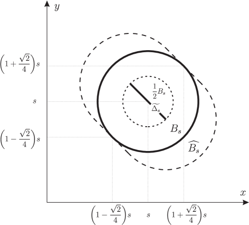
Figure 2. Counterexample for $M_{\mu}^{\mathcal{B}_{+}}$ in dimension $d=2$.

Again, assuming a contrario that $M_{\mu}^{\mathcal{B}_{+}}$ is of weak type $(1,1)$, we claim that

(3.2) $$\mu(\widehat{B_{s}})\lesssim\mu(B_{s}),\qquad s\geq 2.$$

The argument is similar to that for squares. Lemma 2.3 yields

$$\mu(B_{s})=\mu\big{(}B((x^{\prime},y^{\prime}),s/2)\big{)}\simeq\sqrt{s}\,e^{-s(2-\frac{\sqrt{2}}{2})},\qquad s\geq 2,\quad(x^{\prime},y^{\prime})\in\widetilde{\Delta_{s}}.$$

Since $\widehat{B_{s}}$ contains the rectangle $\widetilde{R_{s}}$ with basis $\widetilde{\Delta_{s}}-(\frac{s}{2\sqrt{2}},\frac{s}{2\sqrt{2}})$ and height $s$ (that contains $\frac{1}{2}B_{s}$), we have

$$\mu(\widehat{B_{s}})\geq\int_{\widetilde{R_{s}}}e^{-(x+y)}\,dxdy\gtrsim s\int_{(2-\frac{\sqrt{2}}{2})s}^{(2+\frac{\sqrt{2}}{2})s}e^{-r}\,dr\gtrsim se^{-(2-\frac{\sqrt{2}}{2})s},$$

which for large $s$ contradicts (3.2).

We pass to explaining the changes necessary for $d\geq 3$. Let $Q_{s}$, $s\geq 1$, denote the cube centered at $s\mathbf{1}$, of side length $s$, and let $\widehat{Q_{s}}$ be the union of all cubes emerging from moving the center of $Q_{s}$ along the hypersegment $\Delta_{s}$ obtained by intersecting $\frac{1}{2}Q_{s}$ with the hyperplane $x_{1}+\ldots+x_{d}=ds$. With the present notation the justification of (3.1), assuming a contrario the weak type $(1,1)$ of $M_{\mu}^{\mathcal{Q}_{+}}$, is analogous to that for the case $d=2$ and involves the estimate (see Lemma 2.3)

$$\mu(Q_{s})=\mu\big{(}Q(x^{\prime},s/2)\big{)}\simeq e^{-ds/2},\qquad s\geq 2,\quad x^{\prime}\in\Delta_{s}.$$

Now (3.1) is contradicted for large $s$ by

$$\mu(\widehat{Q_{s}})\gtrsim s^{d-1}e^{-ds/2}.$$

To justify the last estimate, observe that $\widehat{Q_{s}}$ contains the hyperprism $R_{s}$ with basis $\Delta_{s}-\frac{s}{2}\textbf{1}$ and height $\sqrt{d}s$. Then

$$\mu(\widehat{Q_{s}})\geq\int_{R_{s}}e^{-|x|_{1}}\,dx\gtrsim s^{d-1}\int_{\frac{ds}{2}}^{\frac{3ds}{2}}e^{-r}\,dr\gtrsim s^{d-1}e^{-ds/2},\qquad s\geq 1.$$

Similarly, let $B_{s}$, $s\geq 1$, denote the ball with center at $s\textbf{1}$ and radius $s/2$, and let $\widehat{B_{s}}$ be the union of balls emerging from moving the center of $B_{s}$ along the hypersegment $\Delta_{s}$ obtained by intersecting $\frac{1}{2}B_{s}$ with the hyperplane $x_{1}+\ldots+x_{d}=ds$. Assuming again a contrario the weak type $(1,1)$ of $M_{\mu}^{\mathcal{B}_{+}}$, we prove (3.2) in a way analogous to that for the case $d=2$ with the estimate

$$\mu\big{(}B(x^{\prime},s/2)\big{)}\simeq s^{\frac{d-1}{2}}e^{-s(d-\frac{\sqrt{d}}{2})},\qquad s\geq 2,\quad x^{\prime}\in\widetilde{\Delta_{s}}$$

included. Let $\widetilde{R_{s}}$ be the cylinder with basis $\widetilde{\Delta_{s}}-\frac{s}{2\sqrt{d}}$ and height $s$ that includes $\frac{1}{2}B_{s}$. Since $\widetilde{R_{s}}\subset\widehat{B_{s}}$, we have

$$\mu(\widehat{B_{s}})\geq\int_{\widetilde{R_{s}}}e^{-|x|_{1}}\,dx\gtrsim s^{d-1}\int_{(d-\frac{\sqrt{d}}{2})s}^{(d+\frac{\sqrt{d}}{2})s}e^{-r}\,dr\gtrsim s^{d-1}e^{-(d-\frac{\sqrt{d}}{2})s}.$$

For large $s$, this contradicts $\mu(B_{s})\simeq s^{\frac{d-1}{2}}e^{-s(d-\frac{\sqrt{d}}{2})}$. This finishes the proof. ∎

Remark 3.1.

In view of Remark 2.4, the above proof extends in a straightforward manner to the context of the measure $\mu_{\alpha}$ given in (1.1). Consequently, $M_{\mu_{\alpha}}^{\mathcal{Q}_{+}}$ and $M_{\mu_{\alpha}}^{\mathcal{B}_{+}}$ are not weak type $(1,1)$.

Alternative condensed version of the proof of Theorem 1(A), the cases of $\mathbf{M_{\mu}^{\mathcal{Q}}}$ and $\mathbf{M_{\mu}^{\mathcal{B}}}$

Consider first ${M_{\mu}^{\mathcal{Q}_{+}}}$. With $s>1$, we choose $0\leq f\in L^{1}(d\mu)$ so that the measure $fd\mu$ is a close approximation of the Dirac measure $\delta_{2s\mathbf{1}}$. The cube $Q(2s\mathbf{1}+y,s)$ will contain the point $2s\mathbf{1}$ if $y\perp\mathbf{1}$ and $|y|_{\infty}<s$, and this cube is contained in $\mathbb{R}^{d}_{+}$. Then any point $x\in Q(2s\mathbf{1}+y,s)$ will satisfy

(3.3) $$M_{\mu}^{\mathcal{Q}_{+}}f(x)\gtrsim\mu\big{(}Q(2s\mathbf{1}+y,s)\big{)}^{-1}\simeq\exp{\left(|z_{\infty}|_{1}\right)},$$

where we applied Lemma 2.3, and $z_{\infty}=z_{\infty}(2s\mathbf{1}+y,s)=s\mathbf{1}+y$. Notice that $|z_{\infty}|_{1}=ds$ does not depend on $y$. The union of these cubes taken over all admissible points $y$ will contain the set

$$\big{\{}\sigma\mathbf{1}+y:\>s<\sigma<2s,\;y\perp\mathbf{1},\;|y|_{\infty}<s\big{\}},$$

whose $\mu$ measure is at least $c\exp{\left(-|z_{\infty}|_{1}\right)}\,s^{d-1}$. Since (3.3) holds in this set, the weak type $(1,1)$ inequality is violated for large $s$.

In the case of ${M_{\mu}^{\mathcal{B}_{+}}}$, we proceed similarly, with the same $f$ but with the balls $B(2s\mathbf{1}+y,s)$ instead of the cubes. In view of Lemma 2.3, the estimate (3.3) will now read $M_{\mu}^{\mathcal{B}_{+}}f(x)\gtrsim\mu(B(2s\mathbf{1}+y,s))^{-1}\simeq\exp{\left(|z_{2}|_{1}\right)}\,s^{(1-d)/2}$, where $z_{2}=z_{2}(2s\mathbf{1}+y,s)$. The measure of the union of the balls will be at least $c\exp{\left(-|z_{2}|_{1}\right)}\,s^{d-1}$. These two estimates together disprove the weak type inequality. ∎

Proof of Theorem 1(A), the case of $\mathbf{M_{\mu}^{\mathcal{D}}}$

Fixing a large $N>0$, we now let $fd\mu$ approximate $\delta_{(0,\dots,0,N)}$ (cf. the second proof for $M_{\mu}^{\mathcal{Q}_{+}}$).

Let $\xi\in\mathbb{R}^{d}_{+}$ with $|\xi|_{1}<N$, and write $s=|\xi|_{1}$. To estimate $M^{\mathcal{D}_{+}}_{\mu}f(\xi)$ from below, we introduce a closed diamond $D=\{x\in\mathbb{R}^{d}_{+}:|x-c|_{1}\leq M\}$ with $c_{i}=\xi_{i}$ for $i<d$ and $c_{d}=\xi_{d}+M$. Here $M>N+s$. Then the points $\xi$ and $(0,\dots,0,N)$ are both in $D$, and $|x|_{1}\geq s$ if $x\in D$. Since $x_{d}\geq\xi_{d}$ for all points $x\in D$, one has for $h>0$

$$D\cap\{x:\>|x|_{1}=s+h\}\subset \left\{x\in\mathbb{R}^{d}_{+}:\>|x|_{1}=s+h,\;\;\xi_{d}\leq x_{d}\right\}$$

$$\subset \Big{\{}x\in\mathbb{R}^{d}_{+}:\>x_{d}=s+h-\sum_{1}^{d-1}x_{i},\;\;\;\sum_{1}^{d-1}x_{i}\leq s+h-\xi_{d}\Big{\}}$$

and the $(d-1)$-dimensional area of the last set here is $\mathcal{O}((s+h-\xi_{d})^{d-1})$, as seen by projecting onto $\mathbb{R}^{d-1}$. Thus

$$\mu(D)\lesssim\int_{0}^{\infty}(s+h-\xi_{d})^{d-1}e^{-s-h}\,dh\simeq(1+s-\xi_{d})^{d-1}\,e^{-s}.$$

This implies that $M^{\mathcal{D}_{+}}_{\mu}f(\xi)\gtrsim{e^{s}}/(1+s-\xi_{d})^{d-1}$; observe that $s-\xi_{d}=\sum_{1}^{d-1}\xi_{i}$.

Next we choose the level $\lambda={N^{1-d}\,e^{N}}$ and examine when $M^{\mathcal{D}_{+}}_{\mu}f(\xi)\gtrsim\lambda$. This occurs if $1+(s-\xi_{d})^{d-1}\lesssim N^{d-1}e^{s-N}$, in particular if

$$1<N^{d-1}e^{s-N}\quad\mathrm{i.e.}\quad s>N-(d-1)\log N\quad\mathrm{and}\quad(s-\xi_{d})^{d-1}<N^{d-1}e^{s-N}.$$

To find points $\xi\in\mathbb{R}^{d}_{+}$ satisfying these two inequalities, we fix

$$|\xi|_{1}=s\in\big{(}N-(d-1)\log N,\>N\big{)}.$$

We can then choose any $\xi_{i}\in\left(0,\>d^{-1}\,N\,e^{(s-N)/(d-1)}\right)$, $i=1,\dots,d-1$, and set $\xi_{d}=s-\sum_{1}^{d-1}\xi_{i}$. Indeed, for such points $\xi$ the first inequality is clear, and the second one follows because

$$s-\xi_{d}=\sum_{1}^{d-1}\xi_{i}<N\,e^{(s-N)/(d-1)}<s.$$

Here the last inequality assures that $\xi_{d}$ is positive, and it holds since $s<N$ implies $e^{s}\,s^{1-d}<e^{N}\,N^{1-d}$ for large $s$ and $N$.

Keeping still $s$ fixed, we see that the $(d-1)$-dimensional measure of the set of points $\xi$ thus obtained is of order of magnitude $N^{d-1}e^{s-N}$. Varying then $s$, we conclude that the $\mu$-measure of the set of all points $\xi$ obtained is greater than constant times

$$\int_{N-(d-1)\log N}^{N}N^{d-1}e^{s-N}e^{-s}\,ds\simeq N^{d-1}\,e^{-N}\log N=\frac{\log N}{\lambda}.$$

For large $N$, this contradicts the weak-type $(1,1)$ boundedness of $M^{\mathcal{D}_{+}}_{\mu}$. ∎

4. Proof of Theorem 1(B)

As remarked in Section 1, the case of $M_{\mu}^{\mathcal{Q}}$ in Theorem 1(B) is an immediate consequence of the one-dimensional result. The remaining two cases are much less straightforward and will be treated subsequently. We shall work with the operators restricted to $\mathbb{R}^{d}_{+}$, see Proposition 2.1. We make the following two preliminary reductions in proving the $L^{p}$-boundedness of $M_{\mu}^{\mathcal{D}_{+}}$ and ${M_{\mu}^{\mathcal{B}_{+}}}$.

Reduction 1. We may consider only diamonds (elements of $\mathcal{D}_{+}$) or balls (elements of $\mathcal{B}_{+}$) with radii bounded from below by any fixed positive constant, due to the local doubling property of $\mu$, see Lemma 2.2.

Reduction 2. Among diamonds or balls remaining after Reduction 1, we may consider only those not intersecting $t\Sigma_{+}^{d-1}=\{x\in\mathbb{R}^{d}_{+}:|x|_{1}=t\}$ for $0<t\leq c$ with $c>2$ arbitrary and fixed, since otherwise they have measures bounded from below (and above) by a positive constant.

We first consider the simpler case $M^{\mathcal{D}_{+}}_{\mu}$. The reasoning in case of $M^{\mathcal{B}_{+}}_{\mu}$ is more sophisticated, because of the geometry of the balls in $\mathbb{R}^{d}_{+}$, especially those touching the boundary of $\mathbb{R}^{d}_{+}$.

Proof of Theorem 1(B), the case of $\mathbf{M_{\mu}^{\mathcal{D}}}$

Our aim is to prove that $M_{\mu}^{\mathcal{D}_{+}}$ is bounded on $L^{p}(\mathbb{R}^{d}_{+},d\mu)$ for $1<p<\infty$. Recall that diamonds in $\mathbb{R}^{d}_{+}$ are denoted

$$D(z,r) =\big{\{}y\in\mathbb{R}^{d}_{+}:|z-y|_{1}<r\big{\}}.$$

Here $r>0$, and $z$ will always be in $\mathbb{R}^{d}_{+}$.

For each $x\in\mathbb{R}^{d}$ we denote $x_{0}=\sum_{1}^{d}x_{j}$. Then

$$\Pi_{t}=\{x\in\mathbb{R}^{d}:\>x_{0}=t\}$$

is a hyperplane for each $t\in\mathbb{R}$, and we write $\lambda_{t}$ for Lebesgue measure in $\Pi_{t}$. Further, $x_{t}$ will for $t>0$ denote the orthogonal projection on $\Pi_{t}$ of any point $x$.

Let $f$ be a nonnegative function in $L^{1}(d\mu)$, which we extend by $0$ in $\mathbb{R}^{d}\setminus\mathbb{R}^{d}_{+}$. We want to estimate $M_{\mu}^{\mathcal{D}_{+}}f$ at a point $\xi\in\mathbb{R}^{d}_{+}$. So we take a diamond ${D}={D}(z,r)$ with $z\in\mathbb{R}^{d}_{+}$ and such that $\xi\in D$, and estimate the mean

$$\frac{1}{\mu(D)}\,\int_{D}f(y)\,d\mu(y).$$

Reductions 1 and 2 allow us to assume that the quantities $r$ and $z_{0}-r>2$ are large. It will be convenient to write $b=z_{0}-r$, which indicates the “bottom” of the diamond.

Denoting slices of $D$ as $D_{t}=D\cap\Pi_{t}$, we can write this mean as

(4.1) $$\frac{1}{\mu(D)}\,\int_{b}^{b+2r}\,e^{-t}\,\int_{D_{t}}f\,d\lambda_{t}\,dt.$$

The inner integral here will be estimated in terms of a $(d-1)$-dimensional maximal operator. We define $V$ as the set consisting of the $d$-dimensional vector $v=(1,-1,0,\dots,0)$ and all the vectors obtained from $v$ by permuting the coordinates.

Proposition 4.1.

For each $t\in(b,b+2r)$ there exists a $(d-1)$-dimensional parallelepiped $P_{t}\subset\Pi_{t}$ containing $D_{t}$ and containing $\xi_{t}$ such that

$$\lambda_{t}(P_{t})\lesssim\big{[}1+(t-b)\vee(\xi_{0}-b)\big{]}^{d-1}\,e^{b}\,\mu(D)$$

and whose edges are all parallel to vectors in $V$.

Before proving this proposition, we use it to finish the proof of the $L^{p}(d\mu)$-boundedness of $M_{\mu}^{\mathcal{D}_{+}}$. Here $1<p<\infty$.

In the iterated integral in (4.1), we extend the inner integration to $P_{t}$ and insert the factor

$$\frac{[1+(t-b)\vee(\xi_{0}-b)]^{d-1}\,e^{b}\,\mu(D)}{\lambda_{t}(P_{t})}\gtrsim 1.$$

Thus (4.1) is controlled by

$$\int_{b}^{b+2r}\>e^{-t+b}\,[1+(t-b)\vee(\xi_{0}-b)]^{d-1}\,\frac{1}{\lambda_{t}(P_{t})}\,\int_{P_{t}}f\,d\lambda_{t}\,dt.$$

The mean over $P_{t}$ here can be estimated in terms of the non-centered maximal operator $\mathcal{M}_{t}$ in $\Pi_{t}$ associated with parallelepipeds having edges with directions from $V$, evaluated at $\xi_{t}$. So the iterated integral is at most

(4.2) $$\int_{b}^{b+2r}\>e^{-t+b}\,\big{[}1+(t-b)\vee(\xi_{0}-b)\big{]}^{d-1}\,\mathcal{M}_{t}f(\xi_{t})\,dt.$$

We consider the exponent $-t+b$ here. Since $\xi_{0}>b$ and $t>b$, we have

$$-t+b =\frac{\xi_{0}}{p}-\frac{t}{p}-\frac{1}{p^{\prime}}\,(t-b)-\frac{1}{p}\,(\xi_{0}-b)$$

$$\leq\frac{\xi_{0}}{p}-\frac{t}{p}-\Big{(}\frac{1}{p}\wedge\frac{1}{p^{\prime}}\Big{)}\,\big{[}(t-b)\vee(\xi_{0}-b)\big{]}$$

$$\leq\frac{\xi_{0}}{p}-\frac{t}{p}-c\,\big{[}(t-b)\vee(\xi_{0}-b)\big{]}-c\,|\xi_{0}-t|$$

with $c=c(p)>0$; in the last step we used the simple fact that $(t-b)\vee(\xi_{0}-b)\geq|\xi_{0}-t|$. After inserting this estimate in the integral (4.2), we can delete the factors
$e^{-c\,[(t-b)\vee(\xi_{0}-b)]}\,\big{[}1+(t-b)\vee(\xi_{0}-b)\big{]}^{d-1}$, and thus estimate (4.2) by constant times

$$\int_{b}^{b+2r}\>e^{{\xi_{0}}/{p}}\,e^{-{t}/{p}}\,e^{-c\,|\xi_{0}-t|}\,\mathcal{M}_{t}f(\xi_{t})\,dt.$$

Now we apply Hölder’s inequality, with $e^{-c\,|\xi_{0}-t|/p^{\prime}}$ as one factor. It follows that (4.1) is not larger than constant times

$$\bigg{(}\int_{0}^{+\infty}\>e^{{\xi_{0}}}\,e^{-t}\,e^{-c\,|\xi_{0}-t|}\,\big{[}\mathcal{M}_{t}f(\xi_{t})\big{]}^{p}\,dt\bigg{)}^{1/p}.$$

Since this quantity is independent of the choice of the diamond $D$, it gives an upper bound for $M_{\mu}^{\mathcal{D}_{+}}f(\xi)$.

Integrating $p$th powers with respect to $d\mu(\xi)$, one obtains

$$\int\big{[}M_{\mu}^{\mathcal{D}_{+}}f(\xi)\big{]}^{p}\,d\mu(\xi)\lesssim\int_{0}^{+\infty}\int_{\Pi_{t}}\,\int_{0}^{+\infty}\>e^{-t}\,e^{-c\,|\xi_{0}-t|}\,\big{[}\mathcal{M}_{t}f(\xi_{t})\big{]}^{p}\,dt\,d\lambda_{t}(\xi_{t})\,d\xi_{0}.$$

In the right-hand side here, we integrate first in $\xi_{t}$, using the fact^‡ that the operator $\mathcal{M}_{t}$ is bounded on $L^{p}(d\lambda_{t})$ uniformly in $t$. Thus the triple integral is at most constant times

$$\int_{0}^{+\infty}\int_{0}^{+\infty}\>e^{-t}\,e^{-c\,|\xi_{0}-t|}\,\int_{\Pi_{t}}\,\,f(\zeta)^{p}\,d\lambda_{t}(\zeta)\,dt\,d\xi_{0}.$$

Integrating next in $\xi_{0}$, we conclude that

$$\int\big{[}M_{\mu}^{\mathcal{D}_{+}}f(\xi)\big{]}^{p}\,d\mu(\xi)\lesssim\int_{0}^{+\infty}\,e^{-t}\,\int_{\Pi_{t}}\,\,f(\zeta)^{p}\,d\lambda_{t}(\zeta)\,dt=\|f\|_{L^{p}(d\mu)}^{p},$$

and this proves the $L^{p}(d\mu)$-boundedness of $M_{\mu}^{\mathcal{D}_{+}}$.

Proof of Proposition 4.1.

We fix $\xi\in D$ and $t\in(b,b+2r)$, and for convenience we also write $t=b+h=z_{0}-r+h$ with $0<h<2r$. Further, we renumber the coordinates so that

(4.3) $$z_{d}=\max_{1\leq j\leq d}z_{j}.$$

Denote

$$G_{t,\xi}=\Pi_{t}\cap\big{\{}x\in\mathbb{R}^{d}\colon\forall i\;\;x_{i}>-|t-\xi_{0}|\quad\mathrm{and}\quad|z-x|_{1}<r+|t-\xi_{0}|\big{\}}.$$

Obviously $D_{t}\subset G_{t,\xi}$ but also $\xi_{t}\in G_{t,\xi}$. Indeed, $(\xi_{t})_{i}>(\xi_{t})_{i}-\xi_{i}\geq-|\xi_{t}-\xi|_{1}=-|t-\xi_{0}|$ and $|z-\xi_{t}|_{1}\leq|z-\xi|_{1}+|\xi-\xi_{t}|_{1}<r+|t-\xi_{0}|$.

In order to include $G_{t,\xi}$ in a parallelepiped in $\Pi_{t}$, we let $x\in G_{t,\xi}$. Since $|z-x|_{1}<r+|t-\xi_{0}|$ and $(z-x)_{0}=r-h$, we then have for each $i=1,\ldots,d$

(4.4) $$x_{i}-z_{i}\leq\sum_{1}^{d}(x_{i}-z_{i})_{+}=\frac{1}{2}\,\big{[}|x-z|_{1}-(z-x)_{0}\big{]}<\frac{1}{2}\,\big{(}h+|t-\xi_{0}|\big{)}.$$

Switching coordinates to $y_{i}=z_{i}-x_{i}+(h+|t-\xi_{0}|)/2$, we get

$$0<y_{i}<z_{i}+|t-\xi_{0}|+(h+|t-\xi_{0}|)/2=z_{i}+\big{(}h+3|t-\xi_{0}|\big{)}/2,\qquad i=1,\dots,d.$$

Further, $(z-x)_{0}=r-h$ implies, since $y_{d}>0$,

$$\sum_{1}^{d-1}y_{i}=y_{0}-y_{d}=(z-x)_{0}+\frac{d(h+|t-\xi_{0}|)}{2}-y_{d}<r-h+\frac{d(h+|t-\xi_{0}|)}{2}.$$

We need a simple lemma.

Lemma 4.2.

Let $m\geq 2$ and consider the set $E\subset\mathbb{R}^{m}$ defined by

$$E=\Big{\{}y\in\prod_{1}^{m}(0,a_{i}):\,\sum_{1}^{m}y_{i}<R\Big{\}}$$

for some $a_{i},\>R>0$. Then $E$ is contained in the $m$-dimensional rectangle

$$\widetilde{E}=\prod_{1}^{m}(0,a_{i}\wedge R),$$

and the Lebesgue measures satisfy $|E|\simeq\big{|}\widetilde{E}\big{|}=\prod_{1}^{m}a_{i}\wedge R$.

(In expressions like the last product here, we always mean the product of the minima.)

To get the lower estimate for $|E|$ in the lemma, one observes that $E\supset\prod_{1}^{m}(0,(a_{i}\wedge R)/m)$, and the other parts are trivial.

Let the projection $\tau_{t}\colon\Pi_{t}\to\mathbb{R}^{d-1}$ be given by suppression of the last coordinate. The lemma, applied with $m=d-1$ and in the coordinates $(y_{1},\dots,y_{d-1})$, implies that the projection $\tau_{t}(G_{t,\xi})$ is contained in a rectangle $\widetilde{E}$ in $\mathbb{R}^{d-1}$ with sides parallel to the $y$ (or equivalently $x$) coordinate axes. Then $G_{t,\xi}$ is contained in $\tau_{t}^{-1}\big{(}\widetilde{E}\big{)}$, which is seen to be a parallelepiped $P_{t}$ fulfilling the conditions of Proposition 4.1, except that the estimate we get for its Lebesgue measure is

$$\lambda_{t}(P_{t}) \simeq\prod_{1}^{d-1}\bigg{(}z_{i}+\frac{h+3|t-\xi_{0}|}{2}\bigg{)}\wedge\bigg{(}r-h+\frac{d(h+|t-\xi_{0}|)}{2}\bigg{)}$$

(4.5) $$\lesssim\prod_{1}^{d-1}\big{[}z_{i}+h+(t-b)\vee(\xi_{0}-b)\big{]}\wedge r.$$

In addition to (4.5), we will deduce a similar estimate by writing first

$$\sum_{1}^{d-1}x_{i}=z_{0}-(z-x)_{0}-x_{d}<z_{0}-r+h+|t-\xi_{0}|.$$

Combining this estimate with (4.4) and applying Lemma 4.2 in the coordinates $y_{i}=x_{i}+|t-\xi_{0}|$, we can argue as above. As a result, we find a parallelepiped $P_{t}$ containing $G_{t,\xi}$ and verifying

(4.6) $$\lambda_{t}(P_{t})\lesssim\prod_{1}^{d-1}\big{[}z_{i}+h+(t-b)\vee(\xi_{0}-b)\big{]}\wedge\big{(}z_{0}-r+h+|t-\xi_{0}|\big{)}.$$

Next we derive two different lower estimates for $\mu(D)$, whose validity will depend on the condition

(4.7) $$\sum_{1}^{d-1}z_{i}\geq r-h.$$

We shall verify that

(4.8) $$\mu(D)\gtrsim e^{-b}\,\prod_{1}^{d-1}(z_{i}+1)\wedge\bigg{\{}\begin{matrix}r\\ z_{0}-r\end{matrix}\bigg{\}}$$

when (4.7) holds (upper), and when (4.7) is false (lower), respectively.

These two estimates will end the proof of Proposition 4.1 when combined with (4.5) and (4.6), respectively, since

$$\frac{z_{i}+h+(t-b)\vee(\xi_{0}-b)}{z_{i}+1}\lesssim 1+(t-b)\vee(\xi_{0}-b),$$

and

$$\frac{[z_{i}+h+(t-b)\vee(\xi_{0}-b)]\wedge(z_{0}-r+h+|t-\xi_{0}|)}{(z_{i}+1)\wedge(z_{0}-r)}\lesssim 1+(t-b)\vee(\xi_{0}-b);$$

recall here that $z_{0}-r>2$, see Reduction 2.

To verify (4.8), it is enough to show that for $1<h<2$, under relevant assumptions,

(4.9) $$\lambda_{b+h}(D_{b+h})\gtrsim\prod_{1}^{d-1}(z_{i}+1)\wedge\bigg{\{}\begin{matrix}r\\ z_{0}-r\end{matrix}\bigg{\}},$$

because one can then integrate with respect to $e^{-b-h}\,dh$ over the interval $(1,2)$.

Observe that the last coordinate of any point $x\in\Pi_{b+h}$ is given by

(4.10) $$x_{d}=z_{d}+\sum_{1}^{d-1}(z_{i}-x_{i})-r+h=z_{0}-\sum_{1}^{d-1}x_{i}-r+h.$$

Let $h\in(1,2)$. Aiming at the lower case in (4.9) and thus assuming (4.7) false, we define the set

$$E=\bigg{\{}(x_{i})_{1}^{d-1}\in\mathbb{R}^{d-1}:\>0<x_{i}<z_{i}+\frac{h}{2d},\;\;i=1,\dots,d-1,\;\;\,\mathrm{and}\;\;\;\sum_{1}^{d-1}x_{i}<z_{0}-r\bigg{\}}.$$

We claim that the inverse projection, or lift, $\tau_{b+h}^{-1}(E)$ is contained in $D_{b+h}$. Indeed, let $x\in\tau_{b+h}^{-1}(E)$ and consider the last coordinate $x_{d}$ of $x$. From (4.10) we conclude

$$x_{d}>z_{0}-(z_{0}-r)-r+h=h\qquad\mathrm{and}\qquad x_{d}<z_{0}-r+h<z_{d},$$

the last step since (4.7) is false. Thus $x\in\mathbb{R}^{d}_{+}\cap\Pi_{b+h}$. Further,

(4.11) $$|x-z|_{1}=(z-x)_{0}+2\sum_{1}^{d}(x_{i}-z_{i})_{+}<r-h+\frac{2(d-1)h}{2d}<r,$$

so that $x\in D$. The claim follows.

For the measures, we then get $\lambda_{b+h}(D_{b+h})\geq\lambda_{b+h}(\tau_{b+h}^{-1}(E))\simeq|E|$, where $|\cdot|$ denotes Lebesgue measure in $\mathbb{R}^{d-1}$. Lemma 4.2 yields that $|E|\simeq\prod_{1}^{d-1}(z_{i}+1)\wedge(z_{0}-r)$. This proves (4.9) and thus (4.8), for the lower lines.

Next, we verify (4.9) (upper), under the assumption (4.7); recall that $1<h<2$. We start with the case $z_{d}\geq r$, and here we argue almost as above. Define now

$$E^{\prime}=\bigg{\{}(x_{i})_{1}^{d-1}\in\mathbb{R}^{d-1}:\>0<x_{i}<z_{i}+\frac{h}{2d},\;i=1,\dots,d-1,\,\;\mathrm{and}\;\,\sum_{1}^{d-1}x_{i}>\sum_{1}^{d-1}z_{i}-r+h\bigg{\}}.$$

Points in $E^{\prime}$ clearly satisfy

$$-\frac{(d-1)h}{2d}<\sum_{1}^{d-1}(z_{i}-x_{i})<r-h.$$

As before, we take a point $x\in\tau_{b+h}^{-1}(E^{\prime})$ and verify that $x\in D_{b+h}$. From (4.10) combined with $z_{d}\geq r$, we now get

$$x_{d}>z_{d}-(d-1)h/(2d)-r+h>0\qquad\mathrm{and}\qquad x_{d}<z_{d}+r-h-r+h=z_{d}.$$

It follows that $x\in\mathbb{R}^{d}_{+}\cap\Pi_{b+h}$ and that (4.11) remains valid. This proves the inclusion $\tau_{b+h}^{-1}(E^{\prime})\subset D_{b+h}$.

Thus $\lambda_{b+h}(D_{b+h})\gtrsim|E^{\prime}|$, and $|E^{\prime}|$ can be estimated by means of Lemma 4.2 and the coordinates $y_{i}=z_{i}-x_{i}+h/(2d),\;i=1,\dots,d-1$. Since $0<y_{i}<z_{i}+h/(2d)\simeq z_{i}+1$ for each $i$ and $\sum_{1}^{d-1}y_{i}<r-h+(d-1)h/(2d)\simeq r$, the result is $|E^{\prime}|\simeq\prod_{1}^{d-1}(z_{i}+1)\wedge r$. This proves (4.9) (upper) when $z_{d}\geq r$.

In the complementary case $z_{d}<r$, we can suppress $\wedge r$ in (4.9) (upper) because of (4.3). Define $s,\sigma\in\mathbb{R}$ by

$$s\,\sum_{1}^{d-1}\Big{(}z_{i}+\frac{h}{2d}\Big{)}=\sum_{1}^{d-1}z_{i}-r+h,\qquad\sigma\,\sum_{1}^{d-1}\Big{(}z_{i}+\frac{h}{2d}\Big{)}=z_{0}-r.$$

They satisfy $0\leq s<\sigma<1$, where the first inequality follows from (4.7), the second because $h<2<z_{d}$ and the third from $z_{d}<r$. Consider now the set

$$S=\bigg{\{}x\in\Pi_{b+h}\colon s\Big{(}z_{i}+\frac{h}{2d}\Big{)}<x_{i}<\sigma\Big{(}z_{i}+\frac{h}{2d}\Big{)},\;\;i=1,\dots,d-1\bigg{\}}.$$

Clearly, any point $x\in S$ satisfies

$$\sum_{1}^{d-1}z_{i}-r+h<\sum_{1}^{d-1}x_{i}<z_{0}-r,$$

so for its last coordinate, (4.10) implies $0<h<x_{d}<z_{d}$. Thus $S\subset\mathbb{R}^{d}_{+}$, and (4.11) holds again, since for each $i=1,\dots,d-1$

$$x_{i}-z_{i}<(\sigma-1)z_{i}+\sigma h/(2d)<h/(2d).$$

It follows that $S\subset D_{b+h}$.

For the measures, we have

$$\lambda_{b+h}(S)\simeq\big{|}\tau_{b+h}(S)\big{|}=\prod_{1}^{d-1}(\sigma-s)\Big{(}z_{i}+\frac{h}{2d}\Big{)}\simeq(\sigma-s)^{d-1}\,\prod_{1}^{d-1}(z_{i}+1).$$

To finish the proof of (4.9) (upper), it is enough to verify that $\sigma-s\gtrsim 1$. But

$$\sigma-s=\frac{z_{d}-h}{\sum_{1}^{d-1}[z_{i}+h/(2d)]}\gtrsim\frac{z_{d}}{\sum_{1}^{d-1}z_{i}+1}\gtrsim 1,$$

the last inequality because of (4.3). Proposition 4.1 is proved. ∎

Proof of Theorem 1(B), the case of $\mathbf{M_{\mu}^{\mathcal{B}}}$

Our strategy of proving the $L^{p}$-boundedness of ${M_{\mu}^{\mathcal{B}_{+}}}$ is heavily inspired by [10]. Thus we first rotate suitably the whole situation and then use a slicing argument together with $L^{p}$-boundedness of certain standard maximal functions. The details are as follows.

Rotate simultaneously the cone $\mathbb{R}^{d}_{+}$ and all the objects considered (measure, truncated balls, etc.) so that the rotation of $\Sigma_{+}^{d-1}$ is orthogonal to the first coordinate axis and contained in the half-space $\{x\in\mathbb{R}^{d}:x_{1}>0\}$. Then denote by $C_{+}$ the rotated open cone, in which the rotated measure is, up to a multiplicative constant and scaling,

$${\nu}(dx)=e^{-x_{1}}\,dx.$$

Clearly, the above formula extends $\nu$ from $C_{+}$ to all of $\mathbb{R}^{d}$. We shall sometimes use this extension without explicit indication. Further, denote

$$\pi_{\xi}=\{x\in\mathbb{R}^{d}:x_{1}=\xi\},\qquad\xi\geq 0.$$

Our aim is to prove that $M_{\mu}^{\mathcal{B}_{+}}$ is bounded on $L^{p}(\mathbb{R}^{d}_{+},d\mu)$ for $1<p<\infty$. After rotation and scaling and keeping the same symbols, we consider $M_{\mu}^{\mathcal{B}_{+}}$ as a maximal operator acting on functions living on $C_{+}$, related to the family $\widetilde{\mathcal{B}}_{+}$ of truncated Euclidean balls in $\mathbb{R}^{d}$ with centers in $C_{+}$, the truncation being relative to $C_{+}$. Then the $L^{p}$-boundedness concerns $L^{p}(C_{+},d\nu)$.

Thus it is enough that we prove the $L^{p}(d\nu)$-boundedness, $1<p<\infty$, of the maximal operator

(4.12) $$Mf(x)=\sup\frac{1}{\nu(\widetilde{B})}\int_{\widetilde{B}}|f|\,d\nu,$$

where the supremum is taken over all truncated balls

$$\widetilde{B}=\widetilde{B}(m,r):=\mathbf{B}(m,r)\cap C_{+},$$

called simply balls henceforth, such that $m\in C_{+}$ and $x\in\widetilde{B}$. Further, we may assume that $f$ is non-negative and defined in all of $\mathbb{R}^{d}$ but supported in the closure of $C_{+}$.

In what follows points in $\mathbb{R}^{d}$ will be written as $x=(x_{1},x^{\prime})$. We shall always assume that the centers of balls $\widetilde{B}$ are in $C_{+}$. Given $\widetilde{B}$, the minimum

$$\min\big{\{}x_{1}:x\in\operatorname{cl}(\widetilde{B})\big{\}}$$

($\operatorname{cl}$ meaning closure in $\mathbb{R}^{d}$) is taken at a unique point $a=a(\widetilde{B})=(a_{1},a^{\prime})\in\partial\widetilde{B}$.

We now make some preliminary observations that lead to an essential reduction of the class of truncated balls over which the supremum in (4.12) is taken.

Observation 1. We may restrict to balls $\widetilde{B}(m,r)$ with radii uniformly bounded from below by a positive constant, see Reduction 1 above. In addition we may assume that $a_{1}(\widetilde{B})>2$, see Reduction 2.

Observation 2. We may further restrict to balls $\widetilde{B}(m,r)$ such that $a=a(\widetilde{B})\in\partial C_{+}$. (In particular, we exclude untruncated balls $\widetilde{B}=\mathbf{B}(m,r)$ entirely contained in $C_{+}$.) Indeed, if $a\notin\partial C_{+}$, i.e., $a$ is in (the interior of) $C_{+}$, then $m_{1}=a_{1}+r$ and $m^{\prime}=a^{\prime}$, and one considers the following two complementary cases.

If $1\lesssim\sqrt{r}<a_{1}$, then $\nu(\widetilde{B}(m,r))\simeq r^{(d-1)/2}e^{-a_{1}}\simeq\nu(\mathbf{B}(m,r))$ (for the last relation, see the proof of Lemma 2.3) and the result is a simple consequence of [10, Theorem 3].

On the other hand, letting $M_{0}$ be that part of the maximal operator $M$ given by restricting the supremum in (4.12) to balls $\widetilde{B}(m,r)$ remaining after Observation 1 and such that $a(\widetilde{B})\notin\partial C_{+}$ and $a_{1}\leq\sqrt{r}$, we have the following.

Claim: $M_{0}$ is $L^{p}(d\nu)$-bounded for $1<p<\infty$.

To justify the Claim, notice that any $\widetilde{B}$ under consideration contains a cylinder parallel to the $x_{1}$ axis, with one face contained in $\pi_{a_{1}+1}$, of essentially unit width and radius comparable to $a_{1}$, so $\nu(\widetilde{B})\gtrsim a_{1}^{d-1}e^{-a_{1}}$. Given that, consider the projections

$$d\tau(x_{1}) =x_{1}^{d-1}e^{-x_{1}}\,dx_{1},$$

$$F(x_{1}) =\frac{1}{x_{1}^{d-1}}\int_{\pi_{x_{1}}\cap C_{+}}f(x_{1},x^{\prime})\,dx^{\prime},$$

of $d\nu$ and $f$, respectively, on the $x_{1}$ axis (here we omit multiplicative constants, which are irrelevant for the argument). Notice that $\int fd\nu=\int Fd\tau$. Thus we have

$$\frac{1}{\nu(\widetilde{B})}\int_{\widetilde{B}}f\,d\nu\lesssim\frac{1}{\tau(I_{a_{1}})}\int_{I_{a_{1}}}F\,d\tau,$$

where $I_{a_{1}}=(a_{1},\infty)$. Now observe that the one-dimensional maximal operator

$$g(s)\mapsto\sup_{I\ni s}\frac{1}{\tau(I)}\int_{I}g\,d\tau$$

(the supremum taken over all intervals $I\subset\mathbb{R}_{+}$ such that $s\in I$) is of weak type $(1,1)$ with respect to the measure space $(\mathbb{R}_{+},d\tau)$, and it controls $M_{0}$. Therefore $M_{0}$ is of weak type $(1,1)$ with respect to $(C_{+},d\nu)$, and the $L^{p}(d\nu)$-boundedness of $M_{0}$ follows by interpolation with the $L^{\infty}$-boundedness. This finishes proving the Claim and ends Observation 2.

Summing up, in the analysis of (4.12) we may assume that $\widetilde{B}=\widetilde{B}(m,r)$ is a ball such that $m\in C_{+}$ and

(4.13) $$r>\sqrt{d},\qquad a_{1}>2,\qquad a\in\partial C_{+}.$$

By convention, we define the supremum in (4.12) as zero if there is no admissible ball $\widetilde{B}$ containing $x$.

We shall first prove the result in the simplest situation when the dimension $d=2$. This will give us some intuition needed for higher dimensions.

Dimension $\boldsymbol{d=2}$. When $d=2$ we write points simply $x=(x_{1},x_{2})$ rather than $x=(x_{1},x^{\prime})$. Our rotated cone is $C_{+}=\{x\in\mathbb{R}^{2}:|x_{2}|<x_{1}\}$. We can assume that the balls $\widetilde{B}(m,r)$ under consideration are such that $m_{2}\geq 0$, by symmetry. Then $a(\widetilde{B})=(\mathfrak{a},\mathfrak{a})$ with $\mathfrak{a}>2$, and also $r>\sqrt{2}$ and $m_{2}\geq\mathfrak{a}$; see (4.13). Notice that $r/\sqrt{2}<m_{1}-\mathfrak{a}\leq r$ and, of course,

(4.14) $$(m_{1}-\mathfrak{a})^{2}+(m_{2}-\mathfrak{a})^{2}=r^{2}.$$

See Figure 3.

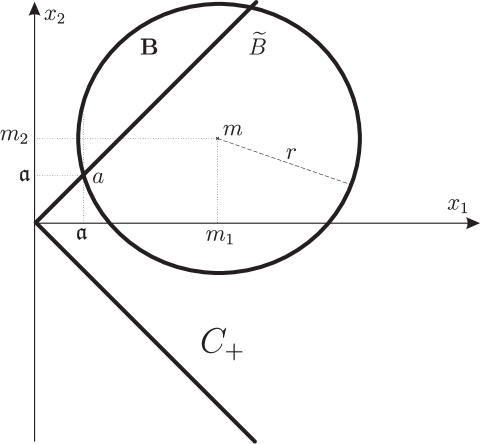
Figure 3. The situation for $d=2$.

We shall now split into cases. In each case, we consider the maximal operator obtained by imposing some conditions on $\widetilde{B}$, in addition to (4.13).

Case 1: $\widetilde{B}$ contains the point $(\mathfrak{a}+1,0)$. Then $\nu(\widetilde{B})\gtrsim\mathfrak{a}e^{-\mathfrak{a}}$, since $\widetilde{B}$ contains a rectangle of unit width and height $\mathfrak{a}$, with one of the vertical edges contained in $\pi_{\mathfrak{a}+1}$. Thus the projection argument from Observation 2 gives the desired conclusion.

Case 2: $\widetilde{B}$ does not contain the point $(\mathfrak{a}+1,0)$. We first find the lower intersection of the line $x_{1}=\mathfrak{a}+h$, $0<h\leq r/\sqrt{2}$, with $\partial\mathbf{B}$, denoted $(\mathfrak{a}+h,\mathfrak{a}-\xi)$; here $\mathbf{B}$ is the untruncated prototype of $\widetilde{B}$ and $\xi=\xi(h)>0$. Notice that the condition defining Case 2 can be written as $\xi(1)\leq\mathfrak{a}$.

We have

$$(m_{1}-\mathfrak{a}-h)^{2}+(m_{2}-\mathfrak{a}+\xi)^{2}=r^{2}.$$

Subtracting (4.14) from this equation leads to

$$\xi^{2}+2(m_{2}-\mathfrak{a})\xi-2(m_{1}-\mathfrak{a})h+h^{2}=0.$$

Dividing by $\xi^{2}$, solving for $1/\xi$ and taking into account that $\xi>0$, we get

$$\xi=\frac{2(m_{1}-\mathfrak{a})h-h^{2}}{m_{2}-\mathfrak{a}+\sqrt{(m_{2}-\mathfrak{a})^{2}+2(m_{1}-\mathfrak{a})h-h^{2}}}.$$

Note that $h<m_{1}-\mathfrak{a}$ (recall that $r/\sqrt{2}\leq m_{1}-\mathfrak{a}<r$). Then $2(m_{1}-\mathfrak{a})h-h^{2}\simeq(m_{1}-\mathfrak{a})h\simeq rh$. Consequently,

(4.15) $$\xi(h)\simeq\frac{rh}{m_{2}-\mathfrak{a}+\sqrt{rh}}\simeq\frac{rh}{m_{2}-\mathfrak{a}}\wedge\sqrt{rh},\qquad 0<h\leq r/\sqrt{2}.$$

To estimate $\nu(\widetilde{B})$ from below, observe that $\widetilde{B}$ contains the triangle $T$ whose vertices are $(\mathfrak{a},\mathfrak{a})$, $(\mathfrak{a}+1,\mathfrak{a}-\xi(1))$ and $(\mathfrak{a}+1,\mathfrak{a})$, and $\nu(T)\simeq\xi(1)e^{-\mathfrak{a}}$. Thus (4.15) implies

(4.16) $$\nu(\widetilde{B})\gtrsim\xi(1)e^{-\mathfrak{a}}\simeq\Big{(}\frac{r}{m_{2}-\mathfrak{a}}\wedge\sqrt{r}\Big{)}e^{-\mathfrak{a}}.$$

Next, we consider all $h>0$ and estimate from above the measures of the intersections $\pi_{\mathfrak{a}+h}\cap\operatorname{shw}\widetilde{B}$, where

$$\operatorname{shw}\widetilde{B}:=\widetilde{B}+\big{(}\mathbb{R}_{+}\times\{0\}\big{)}$$

is the shadow of $\widetilde{B}$ in the positive $x_{1}$ direction. By the geometry of the situation and (4.15), observing also that $m_{2}-\mathfrak{a}<r/\sqrt{2}$, we have

$$\big{|}\pi_{\mathfrak{a}+h}\cap\operatorname{shw}\widetilde{B}\big{|}\leq\begin{cases}\xi(h)+h,&h\leq r/\sqrt{2}\\ 2r,&h>r/\sqrt{2}\end{cases}\Bigg{\}}\lesssim\begin{cases}\frac{rh}{m_{2}-\mathfrak{a}}\wedge\sqrt{rh},&h\leq r/\sqrt{2}\\ r,&h>r/\sqrt{2}\end{cases}\Bigg{\}},\qquad h>0.$$

Using this together with (4.16), by an elementary analysis of cases we see that

(4.17) $$\frac{|\pi_{\mathfrak{a}+h}\cap\operatorname{shw}\widetilde{B}|}{e^{\mathfrak{a}}\nu(\widetilde{B})}\lesssim\begin{cases}\sqrt{h}+h,&h\leq r/\sqrt{2}\\ \sqrt{r}+r,&h>r/\sqrt{2}\end{cases}\Bigg{\}}\lesssim\sqrt{h}+h\lesssim 1+h,\qquad h>0,$$

uniformly in $\mathfrak{a}$ and $\widetilde{B}$.

Now, let $M_{2}$ be the part of the maximal operator (4.12) under consideration, i.e., with the supremum taken only over balls $\widetilde{B}$ considered in Case 2. We will apply the slicing argument from [10].

Similarly as in [10], consider the unit slices

$$S_{i}=\{x\in C_{+}:i<x_{1}\leq i+1\},\qquad i\geq 1.$$

In $S_{i}$ one has $e^{-i-1}dx\leq d\nu(x)\leq e^{-i}dx$. Let

$$M_{2}^{k}f(x)=\sum_{j-i=k}\chi_{S_{j}}(x)M_{2}(f\chi_{S_{i}})(x).$$

Since $M_{2}f\leq\sum_{k\in\mathbb{Z}}M_{2}^{k}f$, it is enough to prove that $\|M_{2}^{k}f\|_{L^{p}(d\nu)}\lesssim 2^{-\delta|k|/p}\|f\|_{L^{p}(d\nu)}$ with some $\delta>0$, because then one can sum the estimates and get the conclusion. Thus we must show that

(4.18) $$\int_{S_{j}}\big{[}M_{2}(f\chi_{S_{i}})\big{]}^{p}\,d\nu\lesssim e^{-\delta|j-i|}\int_{S_{i}}f^{p}\,d\nu,\qquad i,j\geq 1.$$

With $i,j\geq 1$, we let $x\in S_{j}$ and $\widetilde{B}$ be a ball containing $x$, and we will estimate first the mean

$$\frac{1}{\nu(\widetilde{B})}\int_{\widetilde{B}}\chi_{S_{i}}(y)f(y)\,d\nu(y).$$

In our situation $x\in\widetilde{B}\cap S_{j}$ and $y\in\widetilde{B}\cap S_{i}$. Observing that the sets $\{z_{2}\in\mathbb{R}:\exists z_{1}\;(z_{1},z_{2})\in\pi_{\mathfrak{a}+h}\cap\operatorname{shw}\widetilde{B}\}$ form an increasing family of intervals with respect to $h>0$, we get

$$|y_{2}-x_{2}|\leq\big{|}\pi_{i+1}\cap\operatorname{shw}\widetilde{B}\big{|}\vee\big{|}\pi_{j+1}\cap\operatorname{shw}\widetilde{B}\big{|}=\big{|}\pi_{i\vee j+1}\cap\operatorname{shw}\widetilde{B}\big{|};$$

notice that here $i,j\geq 1\vee(\mathfrak{a}-1)=\mathfrak{a}-1$. Then, using (4.17), we obtain

$$\frac{1}{\nu(\widetilde{B})}\int_{\widetilde{B}}\chi_{S_{i}}(y)f(y)\,d\nu(y) \quad\leq\frac{1}{\nu(\widetilde{B})}\int_{i}^{i+1}e^{-i}\int_{|y_{2}-x_{2}|<|{\pi_{i\vee j+1}}\cap\,\operatorname{shw}\widetilde{B}|}f(y_{1},y_{2})\,dy_{2}\,dy_{1}$$

$$\quad\leq 2\,\frac{|{\pi_{i\vee j+1}}\cap\operatorname{shw}\widetilde{B}|}{\nu(\widetilde{B})}\int_{i}^{i+1}e^{-i}\int_{i}^{i+1}\mathcal{M}f(y_{1},x_{2})\,dy_{1}$$

(4.19) $$\quad\lesssim\big{[}1+(i\vee j-\mathfrak{a}+1)\big{]}e^{\mathfrak{a}-i}\int_{i}^{i+1}\mathcal{M}f(y_{1},x_{2})\,dy_{1},$$

where the implicit multiplicative constant is independent of $i,j\geq\mathfrak{a}-1$, the ball $\widetilde{B}$ and the point $x\in\widetilde{B}\cap S_{j}$, and of $f$. Here $\mathcal{M}$ is the one-dimensional non-centered Hardy-Littlewood maximal function acting on the second coordinate. Note that $\mathcal{M}$ is bounded on $L^{p}(\mathbb{R},dx_{2})$ for $p>1$.

We now estimate the factor in front of the integral in (4.19). Write

$$\mathfrak{a}-i-1=\frac{j-i}{p}-\frac{1}{p^{\prime}}(i-\mathfrak{a}+1)-\frac{1}{p}(j-\mathfrak{a}+1)\leq\frac{j-i}{p}-\Big{(}\frac{1}{p}\wedge\frac{1}{p^{\prime}}\Big{)}[i\vee j-\mathfrak{a}+1],$$

where the last inequality follows from the bound $i\wedge j\geq\mathfrak{a}-1$. Thus

$$\big{[}1+(i\vee j-\mathfrak{a}+1)\big{]}e^{\mathfrak{a}-i} \leq e^{j/p-i/p+1}e^{-2\epsilon[i\vee j-\mathfrak{a}+1]}\big{[}1+(i\vee j-\mathfrak{a}+1)]$$

$$\lesssim e^{j/p-i/p}e^{-\epsilon[i\vee j-\mathfrak{a}+1]}$$

$$\leq e^{j/p-i/p}e^{-\epsilon|i-j|},$$

with $\epsilon=\frac{1}{2}(\frac{1}{p}\wedge\frac{1}{p^{\prime}})$, uniformly in $\mathfrak{a}>2$ and $i,j\geq\mathfrak{a}-1$.

With the bound just obtained, taking the supremum of the left-hand side of (4.19) and using Hölder’s inequality on the right-hand side there, we arrive at

$$\chi_{S_{j}}(x)M_{2}(f\chi_{S_{i}})(x)\lesssim e^{j/p-i/p}e^{-\epsilon|i-j|}\chi_{S_{j}}(x)\bigg{(}\int_{i<y_{1}<i+1}\big{[}\mathcal{M}f(y_{1},x_{2})\big{]}^{p}\,dy_{1}\bigg{)}^{1/p}.$$

Raising to power $p$ and integrating this estimate in $x=(x_{1},x_{2})\in S_{j}$ we further get

$$\int_{S_{j}}\big{[}M_{2}(f\chi_{S_{i}})(x)\big{]}^{p}\,e^{-j}dx\lesssim e^{-\epsilon p|j-i|}\int_{i<y_{1}<i+1}\int_{S_{j}}\big{[}\mathcal{M}f(y_{1},x_{2})\big{]}^{p}\,dx_{1}\,dx_{2}\,e^{-i}\,dy_{1}.$$

Finally, we use the $L^{p}$-boundedness of $\mathcal{M}$ to write

$$\int_{\mathbb{R}}\big{[}\mathcal{M}f(y_{1},x_{2})\big{]}^{p}\,dx_{2}\lesssim\int_{\mathbb{R}}f^{p}(y_{1},y_{2})\,dy_{2},\qquad y_{1}\in(i,i+1),$$

and (4.18) with $\delta=\epsilon p$ follows. This finishes the proof in the case of dimension $d=2$.

Remark.

Cases 1 and 2 considered above can be merged. Indeed, right after (4.14) we can estimate $\xi(h)$, as it was done in Case 2, getting (4.15). Then it follows that

$$\nu(\widetilde{B})\gtrsim\big{[}\mathfrak{a}\wedge\xi(1)\big{]}e^{-\mathfrak{a}}\simeq\Big{(}\mathfrak{a}\wedge\frac{r}{m_{2}-\mathfrak{a}}\wedge\sqrt{r}\Big{)}e^{-\mathfrak{a}}.$$

Further, we can estimate measures of the intersections $\pi_{\mathfrak{a}+h}\cap\operatorname{shw}\widetilde{B}$ as (observe that the expression $2(\mathfrak{a}+h)$ appears as the measure of $C_{+}\cap\pi_{\mathfrak{a}+h}$)

$$\big{|}\pi_{\mathfrak{a}+h}\cap\operatorname{shw}\widetilde{B}\big{|} \leq\begin{cases}2(\mathfrak{a}+h)\wedge(\xi(h)+h),&h\leq r/\sqrt{2}\\ 2r,&h>r/\sqrt{2}\end{cases}\Bigg{\}}$$

$$\lesssim\begin{cases}(\mathfrak{a}+h)\wedge\frac{rh}{m_{2}-\mathfrak{a}}\wedge\sqrt{rh},&h\leq r/\sqrt{2}\\ r,&h>r/\sqrt{2}\end{cases}\Bigg{\}},\qquad h>0.$$

Using this together with an elementary analysis of cases we get the key bound

$$\frac{|\pi_{\mathfrak{a}+h}\cap\operatorname{shw}\widetilde{B}|}{e^{\mathfrak{a}}\nu(\widetilde{B})}\lesssim 1+h,\qquad h>0,$$

uniformly in $\mathfrak{a}$ and $\widetilde{B}$. From here the slicing argument goes as described in Case 2 above.

Dimension $\boldsymbol{d=3}$. From now on we will write points $x=(x_{1},x^{\prime})$, with $x_{1}>0$ and $x^{\prime}\in\mathbb{R}^{2}$. Our fixed rotated cone $C_{+}$ is contained in $\mathbb{R}_{+}\times\mathbb{R}^{2}$, its vertex is the origin of $\mathbb{R}^{3}$, and its central axis is the $Ox_{1}$ axis. For any $\xi>0$, the intersection $C_{+}\cap\pi_{\xi}$ is an open equilateral triangle of side $\sqrt{6}\,\xi$.

In order to estimate $Mf$ defined in (4.12), we let $\widetilde{B}=\widetilde{B}(m,r)$ be a truncated ball with $m\in C_{+}$ verifying (4.13).

For any set $E\subset\mathbb{R}^{3}$, we define its shadow in the direction of the $x_{1}$ axis as

$$\operatorname{shw}E:=E+\{(s,0,0):s>0\}.$$

We claim that

(4.20) $$1<r/\sqrt{3}\leq m_{1}-a_{1}\leq r,$$

where only the second inequality needs to be verified. For this we fix $m_{1}$ and $a_{1}$ and use Figure 4.

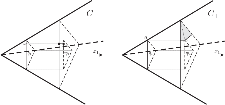
Figure 4. Positions of $a$ and $m$, $d=3$.

Each part of this figure shows the triangles $\pi_{a_{1}}\cap\partial C_{+}$ and $\pi_{m_{1}}\cap\partial C_{+}$, and inside the latter the triangle $\pi_{m_{1}}\cap\operatorname{shw}(\pi_{a_{1}}\cap\partial C_{+})$. Notice that the point $m$ cannot be in the interior of this last triangle, since $a$ is on the boundary of $C_{+}$. Given the position of $a$, the figure illustrates the possible positions of $m$. To the left, $a$ is on an open face of the cone $C_{+}$, and then $m$ is seen to be in the short, closed segment indicated. In the right-hand part of the figure, $a$ is on an edge of $C_{+}$, and $m$ has to belong to the closed quadrilateral marked in the figure. From this, we see that the minimal value of the quotient $(m_{1}-a_{1})/r=(m_{1}-a_{1})/|m-a|$ occurs when $a$ and $m$ are situated on the same edge of $C_{+}$, and then the quotient equals $1/\sqrt{3}$. We have verified the claim (4.20).

For $0\leq h<r+(m_{1}-a_{1})$ we define

$$C_{h}=\big{\{}x^{\prime}\in\mathbb{R}^{2}:(a_{1}+h,x^{\prime})\in C_{+}\big{\}}\qquad\textrm{and}\qquad B_{h}=\big{\{}x^{\prime}\in\mathbb{R}^{2}:(a_{1}+h,x^{\prime})\in\mathbf{B}\big{\}},$$

with $\mathbf{B}=\mathbf{B}(m,r)$. Observe that $B_{h}$ would be empty if defined in this way for $h\geq r+(m_{1}-a_{1})$.

Case I: $a(\widetilde{B})$ lies on an edge of $C_{+}$.

We intersect $C_{+}$ and $\mathbf{B}$ with $\pi_{a_{1}}$, see Figure 5.

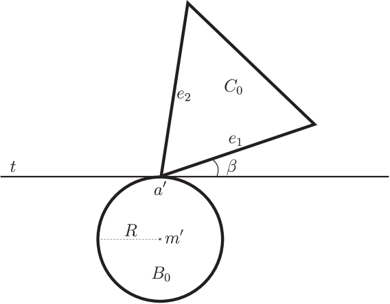
Figure 5. The plane $\pi_{a_{1}}$, $d=3$.

Then $C_{0}$ is an equilateral triangle with one vertex at $a^{\prime}$, and $B_{0}$ is an open disc with center $m^{\prime}$ and radius $R$ satisfying

(4.21) $$(m_{1}-a_{1})^{2}+R^{2}=r^{2}.$$

The definition of $a$ implies that $a^{\prime}\in\partial B_{0}\cap\partial C_{0}$ and also that the tangent line, denoted $t$, to $B_{0}$ through $a^{\prime}$ does not intersect $C_{0}$. Thus $R=|a^{\prime}-m^{\prime}|$.

The point $a^{\prime}$ is the endpoint of two edges of $C_{0}$, and we consider the angles at $a^{\prime}$ between $t$ and these two edges. Let $\beta$ denote the smallest such angle and let $e_{1}$ be the corresponding edge. Then $0\leq\beta\leq\pi/3$, and the other edge $e_{2}$ forms the angle of $\beta+\pi/3$ with the same tangent.

We now consider the intersection of $\mathbf{B}$ and $\operatorname{shw}(C_{+}\cap\pi_{a_{1}})$ with the plane $\pi_{a_{1}+h}$, assuming that $0<h\leq r/\sqrt{3}$; see Figure 6. Then $a^{\prime}$ is an inner point of the disc $B_{h}$.

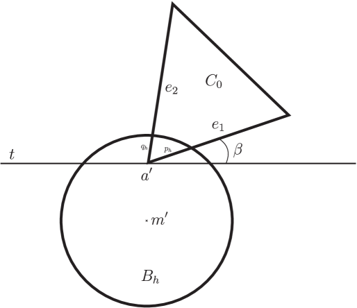
Figure 6. The plane $\pi_{a_{1}+h}$ (formally, here $C_{0}=\operatorname{shw}(C_{+}\cap\pi_{a_{1}})\cap\pi_{a_{1}+1}$),  $d=3$.

From $a^{\prime}$ we move first along the edge $e_{1}$ and then possibly continue beyond it in the same direction until we hit $\partial B_{h}$, say at distance $p_{h}$ from $a^{\prime}$. Then

(4.22) $$(m_{1}-a_{1}-h)^{2}+p_{h}^{2}\cos^{2}\beta+(R+p_{h}\sin\beta)^{2}=r^{2}.$$

Subtracting (4.21), we get

$$p_{h}^{2}+2p_{h}R\sin\beta-2(m_{1}-a_{1})h+h^{2}=0.$$

We rewrite this as a quadratic equation in $1/p_{h}$ which we solve, getting

$$p_{h}=\frac{2(m_{1}-a_{1})h-h^{2}}{\sqrt{R^{2}\sin^{2}\beta+2(m_{1}-a_{1})h-h^{2}}+R\sin\beta}.$$

Since $h\leq r/\sqrt{3}<m_{1}-a_{1}\leq r$, we see that

(4.23) $$p_{h}\simeq\frac{(m_{1}-a_{1})h}{\sqrt{(m_{1}-a_{1})h}+R\sin\beta}\simeq\frac{rh}{\sqrt{rh}+R\sin\beta}\simeq\sqrt{rh}\wedge\frac{rh}{R\sin\beta}.$$

We next repeat the above, but moving in the direction of $e_{2}$ until we leave $B_{h}$, after covering a distance $q_{h}$, say. The same argument applies, but instead of $\beta$ we have $\beta+\pi/3\in[\pi/3,2\pi/3]$. The result is

(4.24) $$q_{h}\simeq\sqrt{rh}\wedge\frac{rh}{R}.$$

We now estimate the measure of $\widetilde{B}$ from below. Consider for the time being only $h\in(1/2,1)$. Then $p_{h}\simeq p_{1}$ and $q_{h}\simeq q_{1}$. Thus we can find one point on each edge $e_{1}$ and $e_{2}$ belonging to the closure of $B_{h}\cap C_{h}$ whose distance from $a^{\prime}$ is comparable to $a_{1}\wedge p_{1}$ and $a_{1}\wedge q_{1}$, respectively (recall that $|e_{1}|=|e_{2}|\simeq a_{1}$). The triangle formed by these two points and $a^{\prime}$ is also contained in $B_{h}\cap C_{h}$ by convexity, and its area is comparable to $(a_{1}\wedge p_{1})(a_{1}\wedge q_{1})$. Integrating over $1/2<h<1$, we see that

(4.25) $$\nu(\widetilde{B})\gtrsim(a_{1}\wedge p_{1})(a_{1}\wedge q_{1})e^{-a_{1}}.$$

Next, we consider all $h\in(0,r+(m_{1}-a_{1}))$. We shall need the following.

Proposition 4.3.

There is an increasing family of parallelograms $\{\mathcal{P}_{h}:0<h<r+(m_{1}-a_{1})\}$ in $\mathbb{R}^{2}$ with sides parallel to $e_{1}$ and $e_{2}$ and side lengths controlled (up to multiplicative absolute constants) by $(a_{1}+h)\wedge p_{h}$ and $(a_{1}+h)\wedge q_{h}$, respectively, in case $0<h\leq r/3$, and by $r$ in case $h>r/3$, such that $B_{h}\cap C_{h}\subset\mathcal{P}_{h}$ for $0<h<r+(m_{1}-a_{1})$.

Proof.

Consider first $h\leq r/3$. The triangle $C_{h}$ is a concentric scaling of $C_{0}$, and all its points have a distance of at most $\sqrt{2}\,h$ from $C_{0}$. In particular, $C_{h}$ has a vertex $a_{h}^{\prime}$, corresponding to $a^{\prime}$, which is at the distance $\sqrt{2}\,h\sin(\beta+\pi/6)$ from $t$, and at the distance $\sqrt{2}\,h\cos(\beta+\pi/6)$ from the line perpendicular to $t$ and passing through $a^{\prime}$ (and $m^{\prime}$); see Figure 7.

Figure 7. The plane $\pi_{a_{1}+h}$ (formally, here $C_{0}=\operatorname{shw}(C_{+}\cap\pi_{a_{1}})\cap\pi_{a_{1}+1}$),  $d=3$.

Bring in the “vertical coordinate”

(4.26) $$\tau(x^{\prime})=\langle x^{\prime}-m^{\prime},a^{\prime}-m^{\prime}\rangle$$

in the plane $\pi_{a_{1}+h}$.

We take as $\mathcal{P}_{h}$ the smallest open parallelogram having one vertex at $a^{\prime}_{h}$, sides parallel to $e_{1}$ and $e_{2}$, and containing $B_{h}\cap C_{h}$. Then we must show that the side lengths of $\mathcal{P}_{h}$ are controlled by $(a_{1}+h)\wedge p_{h}$ and $(a_{1}+h)\wedge q_{h}$. We shall separate the cases depending when $a^{\prime}_{h}$ lies below or above the level of $m^{\prime}$, see Figure 7.

Assume first that $\tau(a^{\prime}_{h})\leq 0$, i.e., $a^{\prime}_{h}$ does not exceed the level of $m^{\prime}$. This means that $\sqrt{2}\,h\sin(\beta+\pi/6)\geq|a^{\prime}-m^{\prime}|=R$, which implies $h\geq R/\sqrt{2}$. In this situation, see (4.23) and (4.24), one has $p_{h}\simeq\sqrt{rh}\simeq q_{h}$. On the other hand, the radius of $B_{h}$ is also comparable with $R+q_{h}\simeq\sqrt{rh}$.

Now, observe that the edges of $\mathcal{P}_{h}$ have lengths controlled by the quantity

$$(\textrm{side length of}\;C_{h})\wedge(\textrm{radius of}\;B_{h}),$$

thus by $(a_{1}+h)\wedge\sqrt{rh}\simeq(a_{1}+h)\wedge p_{h}\simeq(a_{1}+h)\wedge q_{h}$, as desired.

Next, assume that $\tau(a^{\prime}_{h})>0$, i.e., $a^{\prime}_{h}$ is above the level of $m^{\prime}$. We shall construct a parallelogram $\mathcal{P}_{h}^{*}$ containing $\mathcal{P}_{h}$, having vertex at $a^{\prime}_{h}$ and sides parallel to $e_{1}$ and $e_{2}$, whose side lengths satisfy the desired estimates. Clearly, this will be enough for our purpose.

In the plane $\pi_{a_{1}+h}$, let $w$ be the line through $a^{\prime}_{h}$ parallel to $t$. Define $u$ to be the line parallel to $w$ given by $u=\{x^{\prime}:\tau(x^{\prime})=(\sup_{B_{h}}\tau)\wedge(\sup_{C_{h}}\tau)\}$. Observe that two cases may occur (call them (a) and (b), respectively): $u$ is tangent to $B_{h}$ (if the last minimum is realized by $\sup_{B_{h}}\tau$, see Figure 7) or $u$ passes through the vertex of $C_{h}$ of maximal distance from $w$.

The intersection $B_{h}\cap C_{h}$ is contained in the band between $w$ and $u$. In case (a), the width of this band, see Figure 7, is not larger than (actually comparable with) $q_{h}+\sqrt{2}\,h\sin(\beta+\pi/6)$, and this quantity, in view of (4.24), is comparable to $q_{h}$. In case (b), the width of this band is comparable with the side length of $C_{h}$, i.e., with $a_{1}+h$.

Now consider the segment along the $e_{2}$ direction with one endpoint at $a_{h}^{\prime}$, and whose other endpoint lies on $u$. Since $e_{2}$ forms the angle $\beta+\pi/3$ with $u$, which is separated from $0$, the segment in question has length comparable with the width of the band, thus with $(a_{1}+h)\wedge q_{h}$. We take this segment as a side of our $\mathcal{P}_{h}^{*}$.

As the other side of $\mathcal{P}_{h}^{*}$ we shall take the segment along the $e_{1}$ direction with one endpoint at $a_{h}^{\prime}$, and the other endpoint $b_{h}^{\prime}$ lies either on the boundary of $B_{h}$, inside the band, or is the vertex of $C_{h}$ in case $B_{h}$ is so large that $\partial B_{h}$ does not cross this ($e_{1}$-directed) side of $C_{h}$. See again Figure 7. Denote by $\mathfrak{p}_{h}$ the length of this segment. Clearly, $\mathfrak{p}_{h}$ is comparable with $a_{1}+h$ in case $b_{h}^{\prime}$ is the vertex. Assuming the other case $b_{h}^{\prime}\in\partial B_{h}$, we will show that $\mathfrak{p}_{h}$ is comparable to $p_{h}$, a fact that is intuitively clear from the picture. Since $\mathcal{P}_{h}^{*}$ just defined contains^‡ $B_{h}\cap C_{h}$, this will finish the reasoning when $h\leq r/3$.

Observe that, cf. (4.22),

$$(m_{1}-a_{1}-h)^{2}+\big{(}\mathfrak{p}_{h}\cos\beta-\sqrt{2}\,h\cos(\beta+\pi/6)\big{)}^{2}+\big{(}\mathfrak{p}_{h}\sin\beta+R-\sqrt{2}\,h\sin(\beta+\pi/6)\big{)}^{2}=r^{2}.$$

Subtracting (4.21) and solving for $1/\mathfrak{p}_{h}$ (see the analysis leading from (4.22) to (4.23)), we get after some elementary computations and applications of basic trigonometric identities

$$\mathfrak{p}_{h}=\frac{2(m_{1}-a_{1})h+2\sqrt{2}Rh\sin(\beta+\pi/6)-3h^{2}}{\sqrt{R^{2}\sin^{2}\beta+2h(m_{1}-a_{1})+\sqrt{2}Rh\cos\beta-3h^{2}/2}+R\sin\beta-\sqrt{2}\sqrt{3}\,h/2}.$$

Then, recalling that $r/\sqrt{3}<m_{1}-a_{1}\leq r$, $R<r$ and $h\leq r/3$, we arrive at

$$\mathfrak{p}_{h}\simeq\frac{rh}{R\sin\beta}\wedge\sqrt{rh}\simeq p_{h}.$$

Considering $h>r/3$, take as $\mathcal{P}_{h}$ the smallest (open) parallelogram, with sides parallel to $e_{1}$ and $e_{2}$, containing both $\mathcal{P}_{r/3}$ and $B_{m_{1}-a_{1}}$. This parallelogram has side lengths comparable to $r$, by the geometry of the situation.

The fact that the family $\{\mathcal{P}_{h}:h>0\}$ is increasing is clear from the construction. Proposition 4.3 follows. ∎

In view of (4.25), for $\mathcal{P}_{h}$ from Proposition 4.3 we have the bound

$$\frac{|\mathcal{P}_{h}|}{e^{a_{1}}\nu(\widetilde{B})}\lesssim\begin{cases}\frac{[(a_{1}+h)\wedge p_{h}][(a_{1}+h)\wedge q_{h}]}{(a_{1}\wedge p_{1})(a_{1}\wedge q_{1})},&0<h\leq r/3,\\ \frac{r^{2}}{(a_{1}\wedge p_{1})(a_{1}\wedge q_{1})},&h>r/3.\end{cases}$$

To estimate the right-hand side here we use (4.23) and (4.24), and apply an elementary analysis of cases. Considering $h\leq r/3$, if $a_{1}\wedge p_{1}=a_{1}$, then (recall that $a_{1}>2$)

$$\frac{(a_{1}+h)\wedge p_{h}}{a_{1}\wedge p_{1}}\leq\frac{a_{1}+h}{a_{1}}<1+h;$$

if $a_{1}\wedge p_{1}=p_{1}$, then

$$\frac{(a_{1}+h)\wedge p_{h}}{a_{1}\wedge p_{1}}\leq\frac{p_{h}}{p_{1}}\simeq\frac{\frac{rh}{R\sin\beta}\wedge\sqrt{rh}}{\frac{r}{R\sin\beta}\wedge\sqrt{r}}\leq h\vee\sqrt{h}\lesssim 1+h.$$

For $h>r/3$ we have

$$\frac{r}{a_{1}\wedge p_{1}}\simeq\frac{r}{a_{1}\wedge\frac{r}{R\sin\beta}\wedge\sqrt{r}}\leq r\vee(R\sin\beta)\vee\sqrt{r}\lesssim 1+h.$$

The factors involving $q_{h}$ are treated similarly. Thus we arrive at the key bound

(4.27) $$\frac{|\mathcal{P}_{h}|}{e^{a_{1}}\nu(\widetilde{B})}\lesssim 1+h^{2},\qquad h>0,$$

uniformly in $a_{1}$ and $\widetilde{B}$.

We are now in a position to apply the slicing argument. Let $M$ be the part of the maximal operator (4.12) under consideration. As in dimension $2$, we define $S_{i}$ for $i\geq 1$ as $\{x\in C_{+}:i<x_{1}\leq i+1\}$, and in $S_{i}$, $e^{-i-1}dx\leq d\nu(x)<e^{-i}dx$. It is enough to prove that for some constant $\delta>0$

(4.28) $$\int_{S_{j}}\big{[}M(f\chi_{S_{i}})\big{]}^{p}\,d\nu\lesssim e^{-\delta|j-i|}\int_{S_{i}}f^{p}\,d\nu,\qquad i,j\geq 1,$$

see (4.18) and the preceding comments.

To prove (4.28), let $i,j\geq 1$. Let $x\in\widetilde{B}\cap S_{j}$ and $y\in\widetilde{B}\cap S_{i}$. Proposition 4.3 tells us that $x^{\prime}$ and $y^{\prime}$ are contained in a certain parallelogram $\mathcal{P}_{h}$, and both parallelograms are contained in the one given by Proposition 4.3 with $h=(i-a_{1}+1)\vee(j-a_{1}+1)$; notice that here $i,j\geq a_{1}-1$. Define

$$\mathcal{M}^{\prime}g(z)=\sup\frac{1}{|\mathcal{P}|}\int_{\mathcal{P}}|g(w)|\,dw,$$

for any locally integrable function $g$ in $\mathbb{R}^{2}$, where the supremum is taken over all parallelograms $\mathcal{P}$ containing $z$ and with sides parallel to two sides of the triangle $C_{0}$, and $|\mathcal{P}|$ denotes the area of $\mathcal{P}$. Then we can write the estimate

(4.29) $$\frac{1}{\nu(\widetilde{B})}\int_{\widetilde{B}}\chi_{S_{i}}(y)f(y)\,d\nu(y)\leq\frac{1}{\nu(\widetilde{B})}\,e^{-i}\,|\mathcal{P}_{i\vee j-a_{1}+1}|\int_{i}^{i+1}\mathcal{M}^{\prime}f(y_{1},x^{\prime})\,dy_{1}.$$

Note that $\mathcal{M}^{\prime}$ is bounded on $L^{p}(\mathbb{R}^{2})$ for $1<p<\infty$. Indeed, $\mathcal{M}^{\prime}$ splits naturally into three components, each determined by two edges of $C_{0}$. Then a linear transformation makes each component coincide with the strong maximal operator $M_{\mathrm{str}}$ in $\mathbb{R}^{2}$.

Combining (4.29) with (4.27) we obtain

$$\frac{1}{\nu(\widetilde{B})}\int_{\widetilde{B}}\chi_{S_{i}}(y)f(y)\,d\nu(y)\lesssim e^{a_{1}-i}\big{[}1+(i\vee j-a_{1}+1)^{2}\big{]}\int_{i}^{i+1}\mathcal{M}^{\prime}f(y_{1},x^{\prime})\,dy_{1}.$$

This is an analogue of (4.19). From here one proceeds as before, arguing as done after (4.19), getting $L^{p}(d\nu)$-boundedness of the considered part of our maximal operator.

Case II: $a(\widetilde{B})$ lies on a face of $C_{+}$.

Then $a^{\prime}$ is an inner point of a side of the triangle $C_{0}$; see Figure 8.

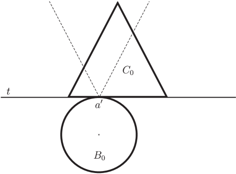
Figure 8. The plane $\pi_{a_{1}}$ in Case II, $d=3$.

We split $C_{0}$ into its intersections with three two-dimensional cones, by introducing two rays from $a^{\prime}$ forming angles of $\pi/3$ with the side of $C_{0}$. Then we apply the arguments from Case I, using instead of $C_{0}$ each of these three intersections, with $\beta=0$ twice and with $\beta=\pi/3$ once, as seen in Figure 8. That intersection which has $\beta=\pi/3$ is not a triangle but a parallelogram. But notice that the $h$-expansion of this parallelogram, analogous to $C_{h}$ in Case I, will necessarily be contained in the analog of the parallelogram $\mathcal{P}_{h}$ constructed in Proposition 4.3. To get the lower estimate (4.25), it is enough to argue as in Case I for the larger of the two intersections with $\beta=0$. In each of the three intersections, we can now follow the pattern of Case I for all upper estimates of integrals, and divide by $\nu(\widetilde{B})$.

This ends the case of dimension $3$.

Dimension $\boldsymbol{d=4}$. We largely follow the three-dimensional argument. Recall that

$$\widetilde{B}=\widetilde{B}(m,r):=\mathbf{B}(m,r)\cap C_{+}.$$

The assumptions (4.13) remain in force. As in dimension three, we define for $0\leq h<r+(m_{1}-a_{1})$

(4.30) $$C_{h}=\big{\{}x^{\prime}\in\mathbb{R}^{3}:(a_{1}+h,x^{\prime})\in C_{+}\big{\}}$$

which is an open regular tetrahedron of side $(a_{1}+h)\,\sqrt{8}$, and

$$B_{h}=\big{\{}x^{\prime}\in\mathbb{R}^{3}:(a_{1}+h,x^{\prime})\in\mathbf{B}(m,r)\big{\}}.$$

Observe that (4.13) implies $a^{\prime}\in\partial C_{0}$. The radius of the ball $B_{h}$ will be denoted by $R_{h}$, and as before we write $R$ for $R_{0}$.

In $\pi_{a_{1}}$, which we identify with $\mathbb{R}^{3}$, we now let $T$ be the tangent plane of the ball $B_{0}$ passing through $a^{\prime}$. Moreover, $T_{+}$ will denote that closed half-space in $\pi_{a_{1}}$ whose boundary is $T$ and which contains $C_{0}$.

Instead of (4.20), we now have

(4.31) $$1<r/2<m_{1}-a_{1}\leq r.$$

The equality (4.21) remains valid and implies

(4.32) $$R^{2}=r^{2}-(m_{1}-a_{1})^{2}=(r+(m_{1}-a_{1}))(r-(m_{1}-a_{1}))\simeq r(r-(m_{1}-a_{1})).$$

When $h<r$, we similarly get for $R_{h}$ in view of (4.31)

(4.33) $$R_{h}^{2}=r^{2}-(m_{1}-a_{1}-h)^{2}=(r+(m_{1}-a_{1}-h))(r-(m_{1}-a_{1})+h)\simeq r(r-(m_{1}-a_{1})+h).$$

We also have

(4.34) $$R_{h}^{2}-R^{2}=(m_{1}-a_{1})^{2}-(m_{1}-a_{1}-h)^{2}=2(m_{1}-a_{1})h-h^{2}\lesssim rh,$$

the last step by (4.31).

The “vertical coordinate” $\tau$ in $\mathbb{R}^{3}$ is defined by (4.26), as in the three-dimensional case.

We will need some angles connected with a regular tetrahedron. The angle at a vertex between an edge and the axis of symmetry from that vertex is $\gamma$, where $\sin\gamma=1/\sqrt{3}$, and the angle between two faces of the tetrahedron is $2\gamma$. Further, the angle between a face and an edge not in that face is $\kappa$, where $\sin\kappa=\sqrt{2/3}$. Using this last angle, one finds that the ratio between the height and the edge of the tetrahedron is $\sqrt{2/3}>1/2$; the height is the distance between a vertex and the opposite face.

Case I: $a^{\prime}$ is a vertex of $C_{0}$.

In $\mathbb{R}^{3}$, the point $a^{\prime}$ is now an endpoint of three edges $e_{1}$, $e_{2}$ and $e_{3}$ of the tetrahedron $C_{0}$. Let $\beta_{i},\;i=1,2,3$, denote the angle at $a^{\prime}$ between $e_{i}$ and the plane $T$. Then $0\leq\beta_{i}\leq\pi/2$, and at most two of the $\beta_{i}$ can be small.

Clearly $a^{\prime}$ is an inner point of the ball $B_{h}$ when $0<h<r+(m_{1}-a_{1})$. We consider for $i=1,2,3$ the intersection of $B_{h}$ and the ray in the direction of $e_{i}$ emanating from $a^{\prime}$. Let $p_{h}^{i}$ be the length of this intersection. We can determine the $p_{h}^{i}$ exactly like $p_{h}$ in dimension three, and instead of (4.23) we get for $0<h<r/2$

(4.35) $$p_{h}^{i}\simeq\sqrt{rh}\wedge\frac{rh}{R\sin\beta_{i}},\qquad i=1,2,3.$$

The argument leading to (4.25) also carries over, so that

(4.36) $$\nu(\widetilde{B})\gtrsim\big{(}a_{1}\wedge p_{1}^{1}\big{)}\,\big{(}a_{1}\wedge p_{1}^{2}\big{)}\,\big{(}a_{1}\wedge p_{1}^{3}\big{)}\,e^{-a_{1}}.$$

As before, $a^{\prime}_{h}$ denotes the vertex of $C_{h}$ that corresponds to $a^{\prime}$; one finds that the distance from $a^{\prime}$ to $a^{\prime}_{h}$ is $\sqrt{3}\,h$.

Let $\mathcal{P}_{h}\subset\mathbb{R}^{3}$ for $0<h\leq r/2$ be the minimal parallelepiped containing $B_{h}\cap C_{h}$ which has one vertex at $a^{\prime}_{h}$ and edges parallel to $e_{1}$,  $e_{2}$ and $e_{3}$. Then $\mathcal{P}_{h}$ increases with $h$.

Proposition 4.4.

For $0<h\leq r/2$, the sides of $\mathcal{P}_{h}$ are bounded by constant times $(a_{1}+h)\wedge p_{h}^{i}$,  $i=1,2,3$.

To prove this, we fix $h\in(0,r/2]$ and deal first with the simple case when $h\geq c_{0}R$, for some small constant $c_{0}>0$ to be determined. Then the $p_{h}^{i}$ are all of magnitude $\sqrt{rh}$, and (4.34) implies

$$R_{h}^{2}\lesssim R^{2}+rh\lesssim rh,$$

the last step since here $R\lesssim h$. Thus $R_{h}\lesssim\sqrt{rh}$.

Comparing the sides of $\mathcal{P}_{h}$ with the minimum of $R_{h}$ and the side of $C_{h}$, we arrive at the conclusion of the proposition, when $h\geq c_{0}\,R$.

Consider now the remaining case $0<h<c_{0}R$, and observe that then $a^{\prime}_{h}\in B_{h}.$ Let $i\in\{1,2,3\}$. We define $\rho_{i}$ as the ray parallel with $e_{i}$, with endpoint at $a^{\prime}_{h}$ and contained in the half-space $\{x^{\prime}:\tau(x^{\prime})\geq\tau(a^{\prime}_{h})\}$. If $\sin\beta_{i}\geq 1/32$, we denote by $b^{\prime}_{i}$ the point of intersection of $\rho_{i}$ and $\partial H$, where $H$ is the half-space

$$H=\Big{\{}x^{\prime}:\tau(x^{\prime})\leq\sup_{B_{h}}\tau\Big{\}}.$$

When $\sin\beta_{i}<1/32$, we define $b^{\prime}_{i}$ similarly, but now with the intersection point of $\rho_{i}$ and $\partial{B_{h}}$. Finally, let $v_{i}$ be the vector $b^{\prime}_{i}-a^{\prime}_{h}$, which is parallel with $e_{i}$. See Figure 9.

Define now

$$\mathcal{P}^{\prime}_{h}=\left\{a^{\prime}_{h}+\sum_{1}^{3}\alpha_{i}v_{i}:\;0\leq\alpha_{i}\leq 1,\;i=1,2,3\right\},$$

a parallelepiped with one vertex at $a^{\prime}_{h}$ and side lengths $|v_{i}|$. It is increasing in $h$.

We will need the following two lemmas, whose proofs are given after the end of the proof of Proposition 4.4.

Lemma 4.5.

If $0<h<c_{0}R$ with $c_{0}$ small enough, then for $i=1,2,3$

$$|v_{i}|\lesssim{p}_{h}^{i},$$

and if moreover $\sin\beta_{i}<1/32$, then

$$|v_{i}|\geq 4h.$$

Lemma 4.6.

If $0<h<c_{0}R$ with $c_{0}$ small enough, then

$$B_{h}\cap C_{h}\subset\mathcal{P}^{\prime}_{h}.$$

Given these lemmas, and still assuming $0<h<c_{0}R$, let $\mathcal{P}^{\prime\prime}_{h}$ be the minimal parallelepiped with one vertex at $a^{\prime}_{h}$ that contains $C_{h}$. Then the parallelepiped $\mathcal{P}^{*}_{h}=\mathcal{P}^{\prime}_{h}\cap\mathcal{P}^{\prime\prime}_{h}$ will contain $B_{h}\cap C_{h}$ because of Lemma 4.6. From Lemma 4.5 and the fact that the sides of $\mathcal{P}^{\prime\prime}_{h}$ are of order of magnitude $a_{1}+h$, it follows that the sides of $\mathcal{P}^{*}_{h}$ are as stated in Proposition 4.4. The minimality of $\mathcal{P}_{h}$ shows that $\mathcal{P}_{h}\subset\mathcal{P}^{*}_{h}$, and this concludes the proof of Proposition 4.4.

In the proofs of the two lemmas, we will denote by $\omega$ the angle at $a^{\prime}$ between the central axis of $C_{0}$ emanating from $a^{\prime}$ and the plane $T$. Notice that $\omega\gtrsim 1$, since $\omega$ is at least as large as the angle between the central axis and a face of $C_{0}$.

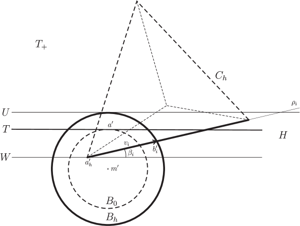
Figure 9. The plane perpendicular to $T$ containing $a^{\prime}_{h}$ and $b^{\prime}_{i}$,  $d=4$.

Proof of Lemma 4.5.

Consider first the case $\sin\beta_{i}\geq 1/32$. The vertical distance $\tau(b^{\prime}_{i})-\tau(a^{\prime}_{h})$ is $R_{h}-R+\sqrt{3}\,h\sin\omega$, see Figure 9. This gives an expression for $|v_{i}|$, and then we use in turn (4.34), (4.33), (4.32) and then (4.35). As a result,

$$|v_{i}|=\frac{R_{h}-R+\sqrt{3}\,h\sin\omega}{\sin\beta_{i}}\lesssim\frac{R_{h}^{2}-R^{2}}{R_{h}}+h\lesssim\frac{rh}{\sqrt{r(r-(m_{1}-a_{1})+h)}}\\ \lesssim\frac{rh}{\sqrt{r(r-(m_{1}-a_{1}))}}\wedge\sqrt{rh}\simeq\frac{rh}{R}\wedge\sqrt{rh}\simeq p_{h}^{i}.$$

In the opposite case $\sin\beta_{i}<1/32$, the quantity $|v_{i}|$ is the length of a segment from $a^{\prime}_{h}$ to a point on $\partial B_{h}$. The segment forms an angle $\beta_{i}$ with the plane $W=\{x^{\prime}:\tau(x^{\prime})=\tau(a^{\prime}_{h})\}$ (and is on the same side of $W$ as the point $a^{\prime}$), as seen in Figure 9.

Project this segment and also the central axis of $C_{h}$ starting at $a^{\prime}_{h}$ orthogonally onto the plane $W$. Let $\theta$ denote the angle between these two projections at their common point $a^{\prime}_{h}$.

Since the endpoint of the segment is on $\partial B_{h}$, the following equation will have the positive solution $z=|v_{i}|$, and also a negative solution. We temporarily write $\ell=R-\sqrt{3}\,h\sin\omega$, which is the vertical distance between $m^{\prime}$ and $a^{\prime}_{h}$. The equation is

$$(\ell+z\sin\beta_{i})^{2}+(-\sqrt{3}\,h\cos\omega+z\cos\beta_{i}\cos\theta)^{2}+(z\cos\beta_{i}\sin\theta)^{2}=R_{h}^{2},$$

or simplified

$$z^{2}+2Kz+L=0,$$

where $K=\ell\sin\beta_{i}-\sqrt{3}\,h\cos\omega\cos\beta_{i}\cos\theta$ and $L=\ell^{2}+3h^{2}\cos^{2}\omega-R_{h}^{2}$. We consider this equation for all $\theta\in[0,\pi]$. Since the two roots of the equation have opposite signs, the constant term $L$ is negative, which can also be seen geometrically. Let us now vary only $\theta$, and write the positive solution as $z=z(\theta)$. Differentiating the equation with respect to $\theta$, we get

$$(z+K)\,\frac{dz}{d\theta}=-z\sqrt{3}\,h\cos\omega\cos\beta_{i}\sin\theta.$$

Since $z$ is the positive solution of the equation, $z+K$ equals the square root that appears in the well-known formula for the solutions, so it is positive. Thus $dz/d\theta<0$ for $0<\theta<\pi$. It follows that the minimal and maximal values of $z(\theta)$ are $z(\pi)$ and $z(0)$, respectively, so that $z(\pi)\leq|v_{i}|\leq z(0)$. We now rewrite the equation with these two values of $\theta$, and replace $K,\>L$ and also $\ell$ by their explicit expressions. Using some elementary trigonometry, one obtains the result

$$z^{2}+2\big{(}R\sin\beta_{i}\pm\sqrt{3}\,h\cos(\omega\pm\beta_{i})\big{)}z-\big{(}R_{h}^{2}-R^{2}+2\sqrt{3}\,Rh\sin\omega-3h^{2}\big{)}=0,$$

where the $\pm$ signs should be read as plus for $z(\pi)$ and minus for $z(0)$. We now solve this equation for $1/z$, denoting

$$K_{*}=R\sin\beta_{i}\pm\sqrt{3}\,h\cos(\omega\pm\beta_{i})\qquad\mathrm{and}\qquad L_{*}=R_{h}^{2}-R^{2}+2\sqrt{3}\,Rh\sin\omega-3h^{2}.$$

The positive solution $z$ is given by

(4.37) $$z=\frac{L_{*}}{K_{*}+\sqrt{K_{*}^{2}+L_{*}}}.$$

We estimate the numerator and the denominator in (4.37) from above and below, choosing $c_{0}$ small enough whenever needed. Because of (4.34), we find

(4.38) $$L_{*}\leq 2rh+4Rh\leq 6rh\lesssim rh$$

and

(4.39) $$L_{*}\geq 2(m_{1}-a_{1})h-4h^{2}\geq rh-4c_{0}rh\geq rh/2,$$

where we also used (4.31). Further, (4.38) implies that

(4.40) $$K_{*}+\sqrt{K_{*}^{2}+L_{*}}\leq 2|K_{*}|+\sqrt{L_{*}}\leq 2R\sin\beta_{i}+2\sqrt{3}\,h+\sqrt{6rh}\leq 2R\sin\beta_{i}+3\sqrt{rh}.$$

From (4.39), we obtain

(4.41) $$K_{*}+\sqrt{K_{*}^{2}+L_{*}}\geq R\sin\beta_{i}-\sqrt{3}\,h+\sqrt{rh/2}\gtrsim R\sin\beta_{i}+\sqrt{rh}.$$

These four inequalities hold whether the $\pm$ signs are read as plus or minus.

Combining (4.38) and (4.41) with (4.37), we conclude that

$$|v_{i}|\lesssim\frac{rh}{R\sin\beta_{i}}\wedge\sqrt{rh}\simeq p_{h}^{i},$$

because of (4.35). If $\sin\beta_{i}<1/32$, (4.39) and (4.40) similarly yield

$$|v_{i}|\geq\frac{rh/2}{2R\sin\beta_{i}+3\sqrt{rh}}\geq\frac{1}{2}\,\frac{rh/2}{(2R\sin\beta_{i})\vee\big{(}3\sqrt{rh}\big{)}}\geq\frac{rh}{8R\sin\beta_{i}}\wedge\frac{\sqrt{rh}}{12}\geq 4h.$$

The last two formulas end the proof of Lemma 4.5. ∎

Proof of Lemma 4.6.

Any point $x\in C_{h}$ can be written $x=a^{\prime}_{h}+\sum_{1}^{3}\alpha_{j}v_{j}$ with $\alpha_{j}\geq 0$. Assume now that $x\in B_{h}\cap C_{h}$. We will show that $\alpha_{j}\leq 1$ for each $j$, so that $x\in\mathcal{P}^{\prime}_{h}$. Thus we fix $j\in\{1,2,3\}$. Observe that to prove the inequality $\alpha_{j}\leq 1$, we may assume that $\alpha_{j}\geq 1$, since the opposite case is clear.

Since $x=a^{\prime}_{h}+\sum_{1}^{3}\alpha_{i}v_{i}\in H$ and the function $\alpha_{i}\mapsto\tau(a^{\prime}_{h}+\sum_{1}^{3}\alpha_{i}v_{i})$ is nondecreasing for each $i$, the point $a^{\prime}_{h}+\alpha_{j}v_{j}$ is also in $H$. If $\sin\beta_{j}\geq 1/32$, this implies $\alpha_{j}\leq 1$, by the definitions of $v_{j}$ and $b^{\prime}_{h}$.

When instead $\sin\beta_{j}<1/32$, we will similarly show that $\alpha_{j}\leq 1$ by proving that $a^{\prime}_{h}+\alpha_{j}v_{j}\in B_{h}$. We know that $a^{\prime}_{h}+\sum_{1}^{3}\alpha_{j}v_{j}\in B_{h}$, so it is enough to verify that the distance $|a^{\prime}_{h}+\sum_{1}^{3}\alpha_{i}v_{i}-m^{\prime}|$ is increasing in $\alpha_{i}$ for $i\neq j$. But

$$\Big{|}a^{\prime}_{h}+\sum_{1}^{3}\alpha_{i}v_{i}-m^{\prime}\Big{|}^{2}\\ =\big{|}a^{\prime}_{h}-m^{\prime}\big{|}^{2}+2\sum_{1}^{3}\alpha_{i}\langle a^{\prime}_{h}-m^{\prime},v_{i}\rangle+\sum_{1}^{3}\alpha_{i}^{2}|v_{i}|^{2}+2\sum_{1\leq i<k\leq 3}\alpha_{i}\alpha_{k}\langle v_{i},v_{k}\rangle,$$

and here all the terms to the right except possibly the second one are nondecreasing in $\alpha_{i}$. Further, $\langle v_{i},v_{k}\rangle=|v_{i}||v_{k}|/2$. Consider for $i\neq j$ the following two terms from the right-hand side

(4.42) $$2\alpha_{i}\langle a^{\prime}_{h}-m^{\prime},v_{i}\rangle+\alpha_{i}\alpha_{j}|v_{i}||v_{j}|.$$

Now

$$\langle a^{\prime}_{h}-m^{\prime},v_{i}\rangle=-\sqrt{3}\,h\cos\omega\,|v_{i}|\cos\beta_{i}+(R-\sqrt{3}\,h\sin\omega)|v_{i}|\sin\beta_{i},$$

so (4.42) equals

$$\alpha_{i}|v_{i}|\left(-2\sqrt{3}\,h\cos\omega\cos\beta_{i}+2\big{(}R-\sqrt{3}\,h\sin\omega\big{)}\sin\beta_{i}+\alpha_{j}|v_{j}|\right).$$

It is enough to verify that the three terms in this parenthesis have a positive sum. The middle term is positive, since $c_{0}$ is small. Recall that we assumed $\alpha_{j}\geq 1$ and also $\sin\beta_{j}<1/32$ which implies $|v_{j}|\geq 4h$ because of Lemma 4.5. Thus the first term in the above parenthesis is dominated by the third term, the parenthesis is positive and the expression in (4.42) is increasing in $\alpha_{i}$, as desired. Lemma 4.6 is proved. ∎

We can now continue Case I as in three dimensions, but using the three quantities ${p}_{h}^{i}$ instead of $p_{h}$ and $q_{h}$. In the estimate (4.27) the exponent of $h$ will be 3 instead of $2$. We extend the definition of $\mathcal{P}_{h}$ by setting it equal to the smallest parallelepiped containing $\mathcal{P}_{r/2}\cap B_{m_{1}-a_{1}}$ for $r/2<h<r+(m_{1}-a_{1})$; cf. the end of the proof of Proposition 4.3 in the three-dimensional case. We leave the details finishing Case I to the reader.

Case II: $a^{\prime}$ is an inner point of a face of $C_{0}$.

This face of $C_{0}$ is contained in the plane $T$, and we consider the three translates $C_{0}^{j},\>j=1,2,3$, of $C_{0}$ along $T$ which have a vertex at $a^{\prime}$ (see Figure 10, where for clarity only that face of $C_{0}$ contained in $T$ is marked).

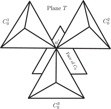
Figure 10. Translates $C_{0}^{j}$ of $C_{0}$, $j=1,2,3$, in Case II,  $d=4$.

The angles at $a^{\prime}$ between $T$ and the edges of each $C_{0}^{j}$ are now $0,\;0,\;\kappa$. The dilations $C_{h}$ are given by (4.30), and we can define for $0\leq h<r+(m_{1}-a_{1})$ analogous dilations $C_{h}^{j},\;j=1,2,3$, of the $C_{0}^{j}$ by replacing in (4.30)  $C_{+}$ by the four-dimensional cone generated by $C_{0}^{j}\times\{a_{1}\}$ and the origin. In analogy with the beginning of Case I, we consider for each $j$ the intersection with $B_{h}$ of the three rays emanating from $a^{\prime}$ and containing an edge of $C_{h}^{j}$. As in Case I, we write $p_{h}^{i},\>i=1,2,3$, for the lengths of these intersections. The $p_{h}^{i}$ will not depend on $j$, and from (4.35) we see that their orders of magnitude are

(4.43) $$\sqrt{rh},\qquad\sqrt{rh}\qquad\mathrm{and}\qquad\sqrt{rh}\wedge\frac{rh}{R}.$$

At least one of the intersections $C_{0}\cap C_{0}^{j},\>j=1,2,3$, is comparable in volume to $C_{0}$. To estimate the measure of $\widetilde{B}$ from below, we can thus for one value of $j$ argue as in Case I with $C_{0}^{j}$ and $C_{h}^{j}$. Hence we still have the lower estimate (4.36). The corresponding upper estimate will now be verified.

In addition to $C_{0}^{j},\>j=1,2,3$, we will consider a finite number of tetrahedra $C_{0}^{j},\,j=4,\dots,N$, of the same size. They will all have a vertex at $a^{\prime}$ and be contained in $T_{+}$. We select them so that the $C_{0}^{j},\,j=1,\dots N$, together cover a neighborhood of $a^{\prime}$ in $T_{+}$. Here $N$ will be an absolute constant. Of the three angles at $a^{\prime}$ between the plane $T$ and an edge of any $C_{0}^{j},\;j=4,\dots,N$, at least one must stay away from 0, since $C_{0}^{j}\subset T_{+}$. (In fact, the largest of these three angles is at least $\pi/4$.) This implies that the corresponding lengths $p_{h}^{i,j}$ (which will now depend also on $j$) have orders of magnitude no larger than those in (4.43).

By $C_{0}^{j,2}$ we denote the result of a scaling of $C_{0}^{j}$ centered at $a^{\prime}$ by a factor of 2. Thus $a^{\prime}$ is a vertex also of $C_{0}^{j,2}$. The $C_{0}^{j,2},\;j=1,\dots,N$, will together contain the intersection of $T_{+}$ and the ball of center $a^{\prime}$ and radius equal to the height of $C_{0}^{j,2}$. Since this height is larger than the diameter, i.e., the edge, of $C_{0}^{j}$, we conclude that

$$\bigcup_{j=1}^{N}\,C_{0}^{j,2}\supset C_{0}.$$

The arguments from Case I will apply to each scaled tetrahedron $C_{h}^{j,2}$. In particular, we choose as there minimal parallelepipeds $\mathcal{P}_{h}^{j}$ containing $B_{h}\cap C_{h}^{j,2},\;\;j=1,\dots,N$, which together cover $B_{h}\cap C_{h}$. The proofs of Lemmas 4.5 and 4.6 and then also that of Proposition 4.4 will go through for each $\mathcal{P}_{h}^{j}$, and this allows us to conclude Case II like Case I.

Case III: $a^{\prime}$ is an inner point of an edge of $C_{0}$.

This edge of $C_{0}$ will be called $e_{0}$. It is contained in $T$, and it is the intersection of two faces of $C_{0}$. We denote by $\Pi^{\prime}$ and $\Pi^{\prime\prime}$ the planes containing these faces. The angle between $\Pi^{\prime}$ and $\Pi^{\prime\prime}$ is $2\gamma$.

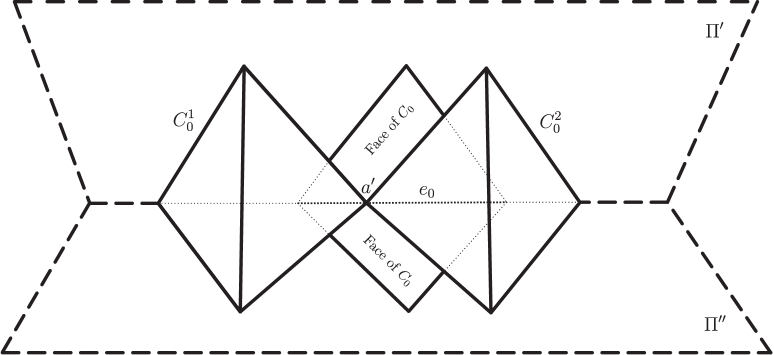
Figure 11. Translates $C_{0}^{j}$ of $C_{0}$, $j=1,2$, in Case III,  $d=4$.

Consider the translates $C_{0}^{1}$ and $C_{0}^{2}$ of $C_{0}$ along $e_{0}$ which have one vertex at $a^{\prime}$ (see Figure 11). Both $C_{0}^{1}$ and $C_{0}^{2}$ have three edges with endpoint $a^{\prime}$: one in $\Pi^{\prime}\cap\Pi^{\prime\prime}$, one in $\Pi^{\prime}$ and one in $\Pi^{\prime\prime}$. These edges form angles with the plane $T$ which are $\beta_{1}=0$,  $\beta_{2}>0$ and $\beta_{3}>0$. For $h\in(0,r+(m_{1}-a_{1}))$ we have dilations $C_{h}$,  $C_{h}^{1}$ and $C_{h}^{2}$ of $C_{0}$, $C_{0}^{1}$ and $C_{0}^{2}$, where the latter two dilations are constructed as in Case II.

Following Case II, we introduce rays emanating from $a^{\prime}$ along the three edges of $C_{0}^{1}$ and $C_{0}^{2}$ and segments of lengths $p_{h}^{i},\>i=1,2,3$. These $p_{h}^{i}$ will satisfy (4.35). At least one of the intersections $C_{0}\cap C_{0}^{1}$ and $C_{0}\cap C_{0}^{2}$ must have volume comparable to that of $C_{0}$. The argument leading to (4.25) can be applied to the corresponding $C_{0}^{j}$; cf. (4.36). This gives the necessary lower estimate for $\nu(\widetilde{B})$.

To get the corresponding upper estimate, we follow the pattern of Case II. We will cover $C_{0}$ by a finite number of (doubled) tetrahedra having one vertex at $a^{\prime}$, among them $C_{0}^{1}$ and $C_{0}^{2}$ doubled. This is done as follows.

Consider the wedge defined as that component of $\mathbb{R}^{3}\setminus\left(\Pi^{\prime}\cup\Pi^{\prime\prime}\right)$ which contains $C_{0}$. There is then a half-plane that splits this wedge in two congruent wedges denoted $V^{\prime}$ and $V^{\prime\prime}$; of these $V^{\prime}$ shall be the one with boundary along $\Pi^{\prime}$.

We will next rotate $C_{0}^{1}$, using as rotation axis the normal through $a^{\prime}$ of the plane $\Pi^{\prime}$. The rotation angle will go from $0$ to $2\pi/3$; the angle $2\pi/3$ will bring $C_{0}^{1}$ to $C_{0}^{2}$. During this rotation, the edge of $C_{0}^{1}$ from $a^{\prime}$ in $\Pi^{\prime}\cap\Pi^{\prime\prime}$ and that in $\Pi^{\prime}$ will both stay in $\Pi^{\prime}$. The edge from $a^{\prime}$ which is in $\Pi^{\prime\prime}$ before the rotation will describe a conic surface, and its angle with $\Pi^{\prime\prime}$ will be positive and increase until it reaches a maximum at the rotation angle $\pi/3$. Then it will decrease back to $0$. This maximum is seen to be $2\gamma-\kappa$, and one has $0<2\gamma-\kappa<\gamma$, the last inequality since $\kappa>\gamma$.

This implies that the rotations of $C_{0}^{1}$ considered will together cover the intersection of $V^{\prime}$ with a neighborhood of $a^{\prime}$. We can then select a finite number of these rotated tetrahedra, say $C_{0}^{j},\>j=1,\dots N$, which together also cover a neighborhood of $a^{\prime}$ in $V^{\prime}$. Notice that $C_{0}^{1}$ and $C_{0}^{2}$ are included here. As in Case II, we consider the doubled tetrahedra $C_{0}^{j,2}$ with a vertex at $a^{\prime}$ and conclude that

$$\bigcup_{j=1}^{N}\,C_{0}^{j,2}\supset C_{0}\cap V^{\prime}.$$

To deal similarly with $V^{\prime\prime}$, we repeat the rotation procedure, swapping $\Pi^{\prime}$ and $\Pi^{\prime\prime}$ as well as $V^{\prime}$ and $V^{\prime\prime}$.

The result will be that we cover $C_{0}$ by a finite number of tetrahedra, each having a vertex at $a^{\prime}$. The edges of these tetrahedra will have angles with $T$ which are larger than or equal to $\beta_{1}$,  $\beta_{2}$ and $\beta_{3}$, respectively. This makes it possible to argue as in Cases I and II, considering dilations $C_{h}$ and $C_{h}^{j,2}$ for $h\in(0,r+(m_{1}-a_{1}))$ and also minimal parallelepipeds.

This ends Case III and the argument in dimension four.

References

- [1] U. Dinger, Weak type (1,1) estimates of the maximal function for the Laguerre semigroup in finite dimensions, Rev. Mat. Iberoamericana 8 (1992), 93–120.
- [2] J. Duoandikoetxea, Fourier Analysis, Grad. Stud. Math. 29, Amer. Math. Soc., Providence, RI, 2001.
- [3] L. Forzani, R. Scotto, P. Sjögren, W. Urbina, On the boundedness of the non-centered Gaussian Hardy-Littlewood maximal function, Proc. Amer. Math. Soc. 130 (2002), 73–79.
- [4] J. Heinonen, Lectures on analysis on metric spaces. Universitext. Springer-Verlag, New York, 2001.
- [5] A. Infante, A remark on the maximal operator for radial measures, Proc. Amer. Math. Soc. 139 (2011), 2899–2902.
- [6] A. Infante, F. Soria, On the maximal operator associated with certain rotational invariant measures, Acta Math. Sin. (Engl. Ser.) 26 (2010), 993–1004.
- [7] N. N. Lebedev, Special functions and their applications, Dover, New York, 1972.
- [8] H.-Q. Li, La fonction maximale non centrée sur les variétés de type cuspidale, J. Funct. Anal. 229 (2005), 155–183.
- [9] H.-Q. Li, Les fonctions maximales de Hardy-Littlewood pour des mesures sur les variétés cuspidales, J. Math. Pures Appl. 88 (2007), 261–275.
- [10] H-Q. Li, P. Sjögren, Y. Wu, Weak type of some operators for the Laplacian with drift, Math. Z. 282 (2016), 623–633.
- [11] A. Nowak, P. Sjögren, T. Z. Szarek, Maximal operators of exotic and non-exotic Laguerre and other semigroups associated with classical orthogonal expansions, Adv. Math. 318 (2017), 307–354.
- [12] E. Sasso, Functional calculus for the Laguerre operator, Math. Z. 249 (2005), 683–711.
- [13] E. Sasso, Maximal operators for the holomorphic Laguerre semigroup, Math. Scand. 97 (2005), 235–265.
- [14] A. Savvopoulou, C. Wedrychowicz, On the weak-type of the uncentered Hardy-Littlewood maximal operator associated with certain measures on the plane, Ark. Mat. 52 (2014), 367–382.
- [15] P. Sjögren, A remark on the maximal function for measures in , Amer. J. Math. 105 (1983), 1231–1233.
- [16] P. Sjögren, F. Soria, Sharp estimates for the non-centered maximal operator associated to Gaussian and other radial measures, Adv. Math. 181 (2004), 251–275.
- [17] A. M. Vargas, On the maximal function for the rotation invariant measures in , Studia Math. 110 (1994), 9–17.