Spin parity effects in monoaxial chiral ferromagnetic chain

Abstract

While spin parity effects– physics crucially depending on whether the spin quantum number $S$ is half-odd integral or integral, have for decades been a source of new developments for the quantum physics of antiferromagnetic spin chains, the investigation into their possible ferromagnetic counterparts have remained largely unchartered, especially in the fully quantum (as opposed to the semiclassical) regime. Here we present such studies for monoaxial chiral ferromagnetic spin chains. We start by examining magnetization curves for finite-sized systems, where a magnetic field is applied perpendicular to the helical axis. For half-odd integer $S$, the curves feature discontinuous jumps identified as a series of level crossings, each accompanied by a shift of the crystal momentum $k$ by an amount of $\pi$. The corresponding curves for integer-valued $S$ are continuous and exhibit crossover processes. For the latter case $k=0$ throughout. These characteristics are observed numerically when the strength of the Dzyaloshinskii-Moriya interaction (DMI) $D$ is comparable to or larger than that of the ferromagnetic exchange interaction $J$. Solitons are known to be responsible for step-wise changes seen in magnetization curves in the classical limit. These findings therefore prompt us to revise the notion of a soliton, for arbitrary $S$, into a quantum mechanical entity.

To unravel this phenomenon at the fully quantum level as is appropriate to spin chains with small $S$, we examine in detail special limiting Hamiltonians amenable to rigorous analysis, consisting of only the DMI and the Zeeman energy. Dubbed the $DH$ model (for $S=1/2$) and the projected $DH$ (p$DH$) model (for general $S$), they have a set of $2S$ conserved quantities, each of which is the number of solitons of a specific integer-valued height (as measured in the $S_{z}$ basis), which ranges from 1 to $2S$. We discuss how to determine the exact crystal momentum of the lowest energy state belonging to a sector with a given set of the $2S$ soliton numbers. Combined with energetic considerations, this information enables us to reproduce the spin parity effect in the magnetization curves. Finally we show that the ground state of the special models have substantial numerical overlap with those for generic systems with a finite exchange interaction, suggesting the same physics to be valid there as well.

I Introduction

It has long been known that an asymmetric exchange interaction, the Dzyaloshinskii-Moriya interaction (DMI)[1, 2], is allowed for pairs of spins bridged with bonds lacking an inversion center. Within a classical treatment of spins, this interaction acts in such a way as to twist the relative orientation of the adjacent spin moments. Owing to this feature, a competition between symmetric exchange interactions and DMI can induce topologically nontrivial configurations such as skyrmions[3, 4, 5, 6, 7, 8] and chiral solitons[9, 10, 11, 12, 13, 14, 15], which will largely behave as stable, particle-like entities with a fixed chirality. That these emergent particles are very much real was demonstrated forcefully in the past decade through Lorentz transmission spectroscopy experiments[7, 13], after which an extensive exploration into their thermodynamics and transport properties ensued.

There exist in the literature studies which highlight the significance of the effect of the DMI on quantum spin systems, e.g. in coupled spin chains modeling CsCuCl₃[16] and in $S=1/2$ antiferromagnetic spin chains modeling Cu-benzoate [17, 18]. It is also true though that the DMI’s role becomes somewhat elusive once one opts for a fully quantum mechanical treatment of the magnet —an essential requirement when $S$, the spin quantum number, is small. This owes to the fact that the notion of a classical spin vector breaks down in this limit, implying that the intuitive understanding deriving from a (semi-)classical picture (valid for sufficiently large $S$) is no longer at our disposal.

Some time ago, Braun and Loss performed their pioneering study on the quantum dynamics of solitons in effectively one dimensional nanomagnets in the absence of a DMI[19]. Though emerging out of a nonchiral magnet, chirality turns out to play an essential role for solitons which are stabilized in such systems by anisotropic interactions. Using semiclassical methods while taking the crucial step of keeping track of spin Berry phases, it was shown how the latter gives rise to spin parity effects – the dependence of the system’s behavior on the parity of twice the spin quantum number 2$S$: the Bloch bands formed by solitons exhibit different structures for integer and half-odd integer $S$, and as a consequence, tunneling between opposite chiralities can occur for the half-odd integer $S$ case. These authors went on to a provide a separate analysis[20] for $S=1/2$ quantum spin chain models (for both ferromagnets and antiferromagnets) with the same symmetry, where within Villain’s approximation[21] of projecting to a fixed soliton number sector, they found results that are consistent with their semiclassical treatment.

Turning to chiral magnets, a similar semiclassical investigation was undertaken by Takashima et al[22] in their work on skyrmion dynamics in 2D chiral ferromagnets, also pointing to a spin parity effect. The major conclusion drawn was that the lowest energy state in the sector with $N_{\rm s}$ skyrmions acquires a crystal momentum of ${\bm{k}}=(2\pi SN_{\rm s},-2\pi SN_{\rm s})$. i.e., ${\bm{k}}$ resides at the zone edge when $SN_{\rm s}$ is half-integral, while being located at the zone center when $SN_{\rm s}$ is integer-valued. It was further argued that the same dichotomy manifests itself when one examines the phase diagram of the system as a function of the applied magnetic field.

Historically, spin parity effects related to topologically nontrivial configurations in quantum spin systems came into focus with the work of Haldane[23, 24] on the spectral properties of antiferromagnetic spin chains. (It is worth mentioning that relations to the crystal momentum of soliton states[23] and hedgehog processes[24] were also briefly addressed in the course of these studies.) The aforementioned body of work suggests that they can arise in a wider range of systems, often with intriguing implications.

With the sole exception of antiferromagnetic spin chains which have been thoroughly scrutinized, it is still largely unknown though, what the full structure of the quantum limit theory and its implications are for most of the problems mentioned above. The present work was motivated largely by the recent advent of the physics of monoaxial chiral ferromagnetic chains[14, 15]. As their analysis to date had mainly been conducted within the (semi-)classical micromagnetic framework, we view the undertaking of its study from a purely quantum perspective an important and urgent task. This explains the purpose of the present work.

In the following sections we will be dealing with quantum spin chains models of chiral ferromagnets for arbitrary $S$. We begin by examining the numerically obtained magnetization curves for the cases $S=1/2,1,3/2$ and $2$. Previously the magnetization curves of finite-sized monoaxial spin chains were calculated in [25] in the classical case, where step-wise changes appearing in the curves were ascribed to solitons. Our numerical results for quantum spin chains show a new feature: a prominent spin parity effect is at play, as detailed in later sections. With the semiclassical picture for solitons unavailable, however, it is not immediately apparent why this should be so. Nor is it obvious what exactly the notion of a soliton becomes when treated as a quantum mechanical entity. We will show that much insight into these problems is gained through the exact study of a limiting case of our full Hamiltonian which we dub the $DH$ model, wherein only the DMI and the Zeeman energy are retained. A variant which we will call the projected $DH$ (p$DH$) model will prove to be invaluable when we turn to the $S>1/2$ cases. These models allow for a clear and rigorous understanding of how the observed spin parity effect can be reproduced in terms of solitons that are well-defined in the quantum limit. While a situation in which the DMI far exceeds the symmetric exchange interaction is admittedly artificial, we will provide numerical evidence strongly suggesting that the $DH$ and p$DH$ models nevertheless capture a generic feature of chiral spin chains.

Perhaps the best way to recap the foregoing paragraph is to view the $DH$ and p$DH$ models as parent Hamiltonians, which generate canonical quantum-soliton states whose exact properties can be utilized to understand the physics of a whole family of generic quantum spin chains. Here we are able to see a parallel structure with the Haldane gap phenomenon in antiferromagnetic spin chains, where the exactly solvable AKLT model[26, 27], acting as the parent Hamiltonian of valence-bond-solid states, played an instrumental role in our understanding of this important spin parity effect at the fully quantum level. In the appendix, we provide a semiclassical account of our problem. While this approach is justified in a parameter regime which is distinct from that of our quantum limit theory, notable similarities in the arguments and outcomes can be detected. This again is reminiscent of the situation for the antiferromagnetic counterpart, where the dual viewpoints deriving from the semiclassical theory of Haldane taken together with the AKLT picture, helped to establish a firmer understanding of the subject. It is worth noting in particular that the quantum picture owing to AKLT has since proved to be essential in bringing this understanding to new heights, where the AKLT state was shown to be a prototype of symmetry-protected-topological states[28], as well as a canonical platform for performing a measurement-based quantum computation[29]. We think that similar developments may well be in store for chiral ferromagnets and their quantum solitons.

We list below our main findings:

• In the $DH$ model for $S=1/2$, the number of solitons $(=N)$ is a good quantum number. A single soliton has a crystal momentum $\pi$ at its minimum energy state. The lowest energy state of the $DH$ model within the sector of states containing $N$ solitons has the crystal momentum $\pi N$. The need to study the general $S$ case naturally lead us to introduce a variant of the $DH$ model (p$DH$ model), in which the numbers of solitons $(=N_{f})$ of height $f=1,2,\cdots 2S$ are all good quantum numbers. Each soliton of height $f$ has the crystal momentum $\pi f$ at its minimum energy state, viz., the existence/absence of a $\pi$-shift in the crystal momentum depends on the parity of the height of each soliton.

• Numerical calculations imply that solely the solitons with maximal height $f=2S$ contribute to the ground states in the p$DH$ model for general $S$. Such energetics, together with the height parity effect conspire to cause the spin parity effect, $k=2\pi SN_{2S}$ in the ground state of the p$DH$ model.

• For $S=1(S=3/2)$, we find a $0.97$ ($0.91$) overlap between the ground state of the $DH$ model and p$DH$ model throughout the relevant range of the magnetic field.

• For $S=1/2(S=1)$, we find that probability of states with one-soliton with height 1 (2) in the ground state for the chiral magnet with $J=D$ is $80\%$ ($58\%$) slightly below the critical field.

The remainder of the paper is organized as follows: In the next section, we explain our model for the monoaxial chiral magnet. Section III discusses numerical results on the magnetization process of finite-sized systems. They will be used to set the issues to be addressed in later sections. Section IV focuses on the study of $S=1/2$ chiral magnets in the limit $J\rightarrow 0$. We turn to higher $S$ cases in Section V. Sections VI and VII are devoted, respectively, to the chirality of quantum solitons and the influence of exchange interactions. Taking stock of what we have learned, in Section VIII, we discuss the implications of the results obtained, offering an intuitive picture for them and pointing to future problems. We state our conclusions in section IX. The appendix discusses how the semiclassical approach applies to the 1d monoaxial chiral magnet. To streamline our discussion, some of the more technical matter are relegated to the Supplemental Material[30], where readers will find the proofs of various lemmas stated in Sections IV and V, and well as detailed calculations that verify several of the results of these sections.

II Model

In this paper we will be concerned with the ground states of quantum spin chain models of monoaxial chiral ferromagnets. Our Hamiltonian in its most complete form reads

$$\hat{\mathcal{H}}_{\rm ch}$$

$$=\sum_{i}\left[-J\hat{\bm{S}}_{i}\cdot\hat{\bm{S}}_{i+1}+D\left(\hat{\bm{S}}_{i}\times\hat{\bm{S}}_{i+1}\right)^{y}-H\hat{S}_{i}^{z}+K\left(\hat{S}_{i}^{y}\right)^{2}\right],$$ (1)

where the $J$-, $D$-, and $H$-terms each stand for the exchange, the Dzyaloshinskii-Moriya and the Zeeman interactions, and the $K$-term is the single ion anisotropy. The chiral axis ($y$-axis) is chosen to coincide with the extent of the spin chain, while the magnetic field is applied perpendicular to it. We set $J$, $H$, $D$, $K$ to be non-negative. Much of the discussions to follow will be devoted to the study of the limit $J=K=0$ in Eq. (1). We will refer to the corresponding Hamiltonian as the $DH$ model:

$$\hat{\mathcal{H}}_{DH}=\hat{\mathcal{H}}_{\rm DM}+\hat{\mathcal{H}}_{\rm Z},$$ (2)

in which

$$\hat{\mathcal{H}}_{\rm DM}=D\sum_{j}\left(\hat{\bm{S}}_{j}\times\hat{\bm{S}}_{j+1}\right)^{y}$$ (3)

$$\hat{\mathcal{H}}_{\rm Z}=-H\sum_{j}\hat{S}_{j}^{z}.$$ (4)

We choose the number of sites $L$ to be even and impose periodic boundary conditions throughout this paper. The wavefunction of a finite-sized spin chain with $L$ sites will be expressed in terms of the ortho-normal basis $|n_{1},n_{2},\cdots,n_{L}\rangle=:|{\bm{n}}\rangle$, where the entries $n_{i}=0,1,\cdots 2S$ ( $i=1,\cdots,L$) are defined through the relation $\hat{S}_{i,z}|\bm{n}\rangle=(S-n_{i})|\bm{n}\rangle$. (We caution the reader that this is therefore not the usual $S_{z}$ basis.) The fully polarized state under a large magnetic field (commonly referred to as the forced ferromagnetic state), for example, is represented by the vector $|00\cdots 00\rangle$. Below, for the sake of clarity, we will often exemplify general discussions on basis vectors in terms of specific spin configurations. The site-translation operator $\hat{T}$ acts on this basis as $\hat{T}|\bm{n}\rangle=|T(\bm{n})\rangle$ where $T(\bm{n}):=(n_{2},n_{3},\cdots,n_{L},n_{1})$. We denote multiple actions of $T$ on $\bm{n}$ by $T^{l}(\bm{n})=T(T^{l-1}(\bm{n}))$ for positive integer $l$. Consider, as a specific example of a basis vector in this representation, the state

$$|00121100012210\rangle.$$ (5)

When acted on by $\hat{T}$, this transforms as

$$\hat{T}|00121100012210\rangle=|00012110001221\rangle.$$ (6)

A word on conventions for site indices: appearances of $n_{i}$ for $i\notin[1,L]$ below are understood to mean $n_{i^{\prime}}$ for $i^{\prime}\in[1,L]$ such that $|i-i^{\prime}|\equiv 0$ (mod $L$). For example, $n_{0},n_{-1}$ and $n_{L+1}$ should each read as $n_{L}$, $n_{L-1}$, and $n_{1}$.

III Numerical results for finite sized systems

Figures 1 and 2 are numerical results for the magnetization curve of finite-sized systems for various spin quantum numbers ($S=1/2,1,3/2,2$). They were obtained through the exact diagonalization of $\hat{\mathcal{H}}_{\rm ch}$. For each $S$ the curves are displayed for the two cases, $D=J$ and $D=50J$. As noted earlier the magnetization curves of finite-sized classical monoaxial spin chains were calculated in [25]. The magnetization for $S=1/2$ and $S=3/2$ exhibit discontinuities as a function of the magnetic field. As indicated in the figures, they correspond to level crossings accompanied by a $\pi$ shift of the crystal momentum. The data for $S=1$ and $S=2$ show a strikingly different behavior. They are continuous and exhibit one or several crossovers. The crystal momentum of the ground state continues to be zero throughout the entire curve.

Motivated by the observation that the features mentioned above persist irrespective of the ratio $D/J$ so long as $D/J\geq 1$, we focus in the following two sections on the limiting case with $J=0$ and finite $D$ (i.e. the $DH$ model (2) and its natural extension to arbitrary $S$, the projected $DH$ (or p$DH$, for short) model, which will appear in Eq.(34).) Remarkably, it turns out that with these models, the mechanism underlying the different behaviors between half-odd integer $S$ and integer $S$ becomes completely tractable. The effect of a finite $J$ is discussed in Sec. VII, following an exact analysis of the $DH$ and p$DH$ models.

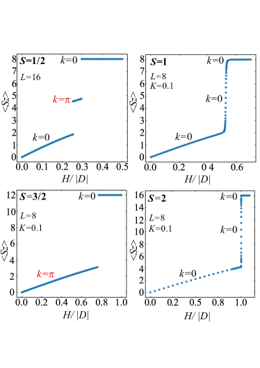
Figure 1: Magnetization curves of finite-sized spin chains for $S=1/2,1,3/2,$ and 2, where we set $D/J=1$.

Figure 2: Magnetization curves of finite-sized spin chains for $S=1/2,1,3/2,$ and 2. Here we have set $D/J=50$.

IV $S=1/2$ model in the limit $J\rightarrow 0$ with finite $D$ .

IV.0.1 Basis and Conserved Quantities

When a periodic boundary condition is imposed on the $DH$ model Eq. (2) for the case $S=1/2$, one can show that the eigenvalue of the operator

$$\hat{N}=\sum_{i=1}^{L}\left(\frac{1}{4}-\hat{S}_{i}^{z}\hat{S}_{i+1}^{z}\right)$$ (7)

is a conserved quantity. One also sees by experimenting with specific examples that this operator counts one half the number of pairs of antiparallel spins occupying adjacent sites. For example,

$$\hat{N}|0001111100\rangle=|0001111100\rangle,$$ (8)

$$\hat{N}|0011100110\rangle=2|0011100110\rangle.$$ (9)

In this section we shall call consecutive entries of $``1"$ in the sea of $``0"$’s a soliton. (Extensions of this notion to higher $S$ cases will be the subject of later sections.) The action of $\hat{N}$ on states can then be regarded as the counting of the soliton number. We denote the set of $\bm{n}$’s such that $\hat{N}|\bm{n}\rangle=N|\bm{n}\rangle$ by $V_{N}$.

To see that Eq. (7) is conserved as announced, we note that the Zeeman energy and $\hat{N}$ can both be expressed in terms of $\{\hat{S}_{i,z}\}$ only. The two quantities therefore commute. The commutativity between $\hat{N}$ and the remaining DMI can also be checked by direct calculation as we now show. To this end, as well as for later discussions, it proves convenient to rewrite the DMI in the following way:

$$\hat{\mathcal{H}}_{\rm DM}=-D\sum_{i=1}^{L}\hat{h}_{i},$$ (10)

where

$$\hat{h}_{i}=\frac{1}{2}\left(\hat{S}_{i+1,z}-\hat{S}_{i-1,z}\right)\left(\hat{S}_{i,+}+\hat{S}_{i,-}\right),$$ (11)

with $\hat{S}_{i,\pm}=\hat{S}_{i,x}\pm i\hat{S}_{i,y}$. Once written in this form, it becomes clear that acting on a state $|\bm{n}\rangle$ with $\hat{h}_{i}$ will result in a null vector unless $n_{i+1}\neq n_{i-1}$. Situations where this non-vanishing condition is met are exhausted by the following four cases:

$$2\hat{h}_{i}|\cdots 0\overset{i}{0}1\cdots\rangle=-|\cdots 0\overset{i}{1}1\cdots\rangle$$ (12a)

$$2\hat{h}_{i}|\cdots 0\overset{i}{1}1\cdots\rangle=-|\cdots 0\overset{i}{0}1\cdots\rangle$$ (12b)

$$2\hat{h}_{i}|\cdots 1\overset{i}{0}0\cdots\rangle=+|\cdots 1\overset{i}{1}0\cdots\rangle$$ (12c)

$$2\hat{h}_{i}|\cdots 1\overset{i}{1}0\cdots\rangle=+|\cdots 1\overset{i}{0}0\cdots\rangle.$$ (12d)

A close inspection of Eqs. (12a)-(12d), reveals that $\hat{h}_{i}$ generates a nonzero state vector when site $i$ is located at the boundary between a soliton $``1111"$ and the background $``0000"$, in which case the new state has a boundary that has been shifted by one site to the left ((12a),(12d)) or to the right ((12b),(12c)). In all four cases the length of the soliton has changed while the number of solitons is preserved. The sum of $\hat{h}_{i}$, Eq. (10) therefore commutes with $\hat{N}$ under a periodic boundary condition.

IV.0.2 Finite size calculation of Magnetization and Spectrum

The left panel of Fig. 3 depicts the magnetization curve of finite-sized systems of the spin $S=1/2$ $DH$ model. Notice that for this model, the ground state is characterized by both the soliton number $N$ and the crystal momentum, as is made explicit in this figure. It is seen that the soliton number $N$ decreases (increases) in a stepwise manner with increasing (decreasing) magnetic field. The dotted line indicates the magnetic field at which the single soliton state $N=1$ is the ground state. The low energy sector of the energy spectrum at this value of the magnetic field is shown in the right panel of Fig. 3. The red dots represent the energy eigenstates with $N=1$, where we see two bands of single soliton states. Both bands have their minimum energy at the crystal momentum $k=\pi$. The blue dots form two continua and one isolated branch. The continua correspond to the scattering states of two soliton excitations. We attribute the isolated branch to the two soliton bound states formed by the repulsive interaction between the solitons. These figures clearly show that the crystal momentum $k$ of the lowest energy state for the sector with the soliton number $N$ is given by $k=\pi N$. We will provide a proof of this generic property in the next subsection.

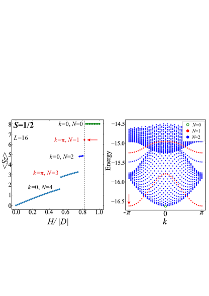
Figure 3: (Left) The magnetization curve of a finite-sized spin chain for the $S=1/2$ $DH$ model with $L=16$. In addition to the crystal momentum $k$, the eigenvalue $N$ of the ground state is shown. The dotted line shows the position on the magnetic field axis at which the $N=1$ state (indicated by the red arrow) is the ground state. (Right) The energy spectrum, i.e., the set of eigenenergy and the crystal momentum of the system with $L=40$. The magnetic field is fixed at the value $H=0.831|D|$, where the $N=1$ state is the ground state. The ground state is indicated by the red arrow. The red and blue points are the eigenstates for which $N=1$ and $N=2$, respectively. The open green circle is an $N=0$ eigenstate.

IV.0.3 Exact results

Theorem 1
Consider those eigenstates of the $S=1/2$ $DH$ model Eq. (2) for which the eigenvalue of $\hat{N}$ is $N$. The crystal momentum of the lowest energy eigenstate is then $k=\pi N$.
 
Definition: Signed basis
We generate a new set of basis states by multiplying each element $|{\bm{n}}\rangle$ of the original basis by the factor $(-1)^{\delta(\bm{n})}$, where

$$\delta(\bm{n})=\sum_{j=1}^{L}j\left(n_{j+1}-n_{j}+|n_{j+1}-n_{j}|\right)/2.$$ (13)

This defines our signed basis. We also define the sign of $\bm{n}$ by $(-1)^{\delta(\bm{n})}$. For instance the signed basis states corresponding to Eqs. (8) and (9) are

$$(-1)^{3} |00\overset{\downarrow}{0}1111100\rangle,$$ (14)

$$(-1)^{2+7} |0\overset{\downarrow}{0}1110\overset{\downarrow}{0}110\rangle,$$ (15)

as depicted in Fig. 4.

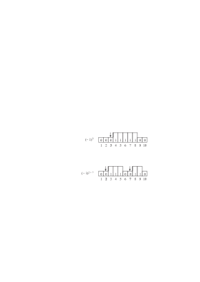
Figure 4: Schematic illustration of the sign $(-1)^{\delta(\bm{n})}$ for $S=1/2$. The symbol $\delta(\bm{n})$ was defined by Eq. (13).

We see that $\delta(\bm{n})$ coincides with the sum of the site indices of the right-most entry of $``0"$ (indicated by arrows) within each segment of the background i.e. consecutive appearances of 0. In the following we will be using the terminology the site index of a $``01"$ boundary. By this we refer to the site index of the $``0"$ immediately to the left of a soliton. Examples of such sites are indicated by arrows in Eqs. (14), (15), and Fig. 4. As a direct consequence of the definition of $\delta(\bm{n})$ given in Eq. (13),

$$(-1)^{\delta(\bm{n})}=(-1)^{\delta(T(\bm{n}))}(-1)^{N}.$$ (16)

Lemma 1 (off-diagonal matrix element)
The off-diagonal matrix elements of $\hat{\mathcal{H}}_{DH}$ Eq. (2) in the signed basis $(-1)^{\delta(\bm{n})}|\bm{n}\rangle$ for $\bm{n}\in V_{N}$ are non-positive.
 
Proof of Lemma 1

Proof.

Since the Zeeman interaction is diagonal in the signed basis, it suffices to show that in this basis all off-diagonal elements of $\hat{\mathcal{H}}_{\rm DM}$, defined by Eq. (10), are non-positive. The actions of the local Hamiltonian $\hat{h}_{i}$ Eqs. (12a)-(12d) can be summarized as

$$2\hat{h}_{i}|\bm{n}\rangle=(n_{i-1}-n_{i+1})|\bar{\bm{n}}^{(i)}\rangle,$$ (17)

where $\bar{\bm{n}}^{(i)}=(\bar{n}^{(i)}_{1}\bar{n}^{(i)}_{2}\cdots\bar{n}^{(i)}_{L})$ and

$$\bar{n}^{(i)}_{j}=\left\{\begin{array}[]{cc}n_{j},&j\neq i\\ 1-n_{i},&j=i\\ \end{array}\right.$$ (18)

In Eqs. (12a) and (12b), where $n_{i-1}-n_{i+1}=-1$, the site indices of the $``01"$ boundary differ by one between $\bm{n}$ and $\bar{\bm{n}}^{(i)}$ and hence $\delta(\bm{n})=\delta(\bar{\bm{n}}^{(i)})\pm 1$. Acting on a signed basis then results in

$$2\hat{h}_{i}(-1)^{\delta(\bm{n})}|\bm{n}\rangle=|n_{i-1}-n_{i+1}|(-1)^{\delta(\bar{\bm{n}}^{(i)})}|\bar{\bm{n}}^{(i)}\rangle.$$ (19)

Notice that the negative matrix elements of Eqs. (12a) and (12b) have now acquired a positive sign upon switching to the signed basis. This can be understood as having come from the opposite signs that $\bm{n}$ and $\bar{\bm{n}}$ possess. The relation Eq. (19) applies as well to Eqs. (12c) and (12d), since in this case $|n_{i-1}-n_{i+1}|=n_{i-1}-n_{i+1}=1$ and the action of $\hat{h}_{i}$ does not move the site indices of the $``01"$ boundary, resulting in $\delta(\bm{n})=\delta(\bar{\bm{n}})$.

It then follows that the off-diagonal matrix elements of $\hat{\mathcal{H}}_{\rm DM}$ Eq. (10) and thus those of $\hat{\mathcal{H}}_{DH}$ are non-positive in the signed basis. ∎

We consider the states that belong to Ker($\hat{\mathcal{H}}_{\rm DM}$), i.e., the eigenspace of $\hat{\mathcal{H}}_{\rm DM}$ for zero energy, and other states separately. The basis states for which $|\bm{n}\rangle\in{\rm Ker}(\hat{\mathcal{H}}_{\rm DM})$ satisfy $n_{i}=n_{i+2}$ for all $i\in[1,L]$, which we can confirm by inspection of the action of the DMI on the basis states as discussed in Lemma 1. Those $|\bm{n}\rangle$ satisfying this condition belong to one of either spaces: $V_{0}=\{000\cdots 000,111\cdots 111\}$ (the states with $N=0$) or $V_{L/2}=\{101\cdots 010,010\cdots 101\}$ (the states with $N=L/2$). Note that these are eigenstates of $\hat{\mathcal{H}}_{DH}$ with eigenenergy $-H\sum_{j=1}^{L}(S-n_{j})$. Among these, the state $|00\cdots 00\rangle$ has the lowest energy and is a simultaneous eigenstate of $\hat{T}$ and $\hat{N}$ with the eigenvalues $k=0$ and $N=0$. Meanwhile the states $|\bm{n}\rangle\notin$ Ker($\hat{\mathcal{H}}_{\rm DM}$) are the eigenstates of $\hat{N}$ with the eigenvalue $N\in[1,L/2-1]$. For those states, the following Lemma holds.  
Lemma 2 (irreducibility)
For arbitrary pairs of $\bm{n}$ and $\bm{n}^{\prime}$ belonging to $V_{N}$ with $N\in[1,L/2-1]$, there exists a positive integer $l$ such that

$$(-1)^{\delta(\bm{n})+\delta(\bm{n}^{\prime})}\langle\bm{n}|(-\hat{\mathcal{H}}_{DH})^{l}|\bm{n}^{\prime}\rangle>0.$$ (20)

Though we defer the proof of Lemma 2 to the Supplemental Material[30], this statement should be intuitively acceptable when one realizes that Eq. (20) holds if multiple actions $\hat{h}_{i^{\prime}}\hat{h}_{i^{\prime\prime}}\hat{h}_{i^{\prime\prime\prime}}\cdots$ of the local Hamiltonians on state $(-1)^{\delta(\bm{n})}|\bm{n}\rangle$ can translate, shorten, and stretch the solitons in the state. Those operations consist of the one-site shift of the $``01"$ boundary and $``10"$ boundary, which can be performed by the local Hamiltonian $\hat{h}_{i}$ as shown in Eqs. (12a)-(12d). Figure 5 shows an example of translation of a single soliton by the multiple action of the local Hamiltonians

$$4\hat{h}_{2}\hat{h}_{4}(-1)^{1}|011000\rangle=(-1)^{2}|001100\rangle+\mbox{other terms}.$$ (21)

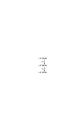
Figure 5: Schematic illustration of a one-site translation of a single soliton. The underlined three sites indicate those allowing the outcome of the action of the local Hamiltonian $\hat{h}_{i}$ on the state to be nonzero.

The first (the second) step in Fig. 5 demonstrates a process where the soliton is stretched (shortened). See the Supplemental Material[30] for a proof.  
 
Proof of Theorem 1

Proof.

When $N\in[1,L/2-1]$, it follows from Lemmas 1 and 2 and the Perron-Frobenius theorem[31] that (1) the lowest energy eigenstate of $\hat{\mathcal{H}}_{DH}$ within each eigenspace of $\hat{N}$ is non-degenerate, and (2) the state vector $|E_{{\rm min},N}\rangle$ of the lowest energy state is spanned by the signed basis, where all coefficients are positive, i.e.,

$$|E_{{\rm min},N}\rangle= \sum_{\bm{n}\in V_{N}}a(\bm{n})(-1)^{\delta(\bm{n})}|\bm{n}\rangle,$$ (22)

with $a(\bm{n})>0.$ Note that the sum over $\bm{n}$ encompasses all $N$ soliton basis states. For $N=1$, e.g. we can write $|E_{{\rm min},1}\rangle$ in the form

$$|E_{{\rm min},1}\rangle= a_{1}(-1)^{1}|010000\rangle+a_{2}(-1)^{2}|001000\rangle+\cdots$$

$$+ b_{1}(-1)^{1}|011000\rangle+b_{2}(-1)^{2}|001100\rangle+\cdots$$

$$+ \cdots$$ (23)

with $a_{i},b_{i}\cdots>0$. Owing to the nondegeneracy of $|E_{{\rm min},N}\rangle$, it is an eigenstate of the site-translation operator $\hat{T}$ and thus

$$|a(\bm{n})|=|a(T(\bm{n}))|,$$ (24)

which leads to $a(\bm{n})=a(T(\bm{n}))$ because of the condition $a(^{\forall}\bm{n}\in V_{N})>0$. We can thus rewrite Eq. (22) as

$$|E_{{\rm min},N}\rangle$$

$$= a(\bm{n})\left((-1)^{\delta(\bm{n})}|\bm{n}\rangle+(-1)^{\delta(T(\bm{n}))}|T(\bm{n})\rangle+\cdots\right)$$

$$+\cdots$$

$$= a(\bm{n})(-1)^{\delta(\bm{n})}\left(|\bm{n}\rangle+(-1)^{N}|T(\bm{n})\rangle+\cdots\right)$$

$$+\cdots$$ (25)

From the the final expression of the above equation, we see that

$$\hat{T}|E_{{\rm min},N}\rangle=(-1)^{N}|E_{{\rm min},N}\rangle$$ (26)

for $N\in[1,L/2-1]$. We have already shown that this relation holds for $N=0$ and the states with $N=L/2$ cannot be the ground state. This concludes our proof. ∎

V Higher $S$ model in the limit $J\rightarrow 0$ with finite $D$

V.0.1 Soliton numbers with various heights and the projected $DH$ model

For $S>1/2$, i.e. when $S=1,3/2,2\cdots$, the $DH$ model has no conserved quantity. However, we have found through finite-sized diagonalization studies that slightly below the critical field, a large weight within the ground state wavefunction is dominated by those basis states which can be interpreted as higher spin versions of single solitons. As an example we display in Eq. (27) a partial list of such dominant states for the case of $S=1$:

$$|00200000\rangle$$

$$|00120000\rangle$$

$$|00210000\rangle$$

$$|00122000\rangle$$

$$|02210000\rangle$$

$$|00211000\rangle$$

$$\quad\quad\vdots$$ (27)

To fully characterize the wider variety of spatial structures that a soliton can exhibit in the higher $S$ cases, we incorporate a set of $2S$ operators $\hat{N}_{1},\cdots,\hat{N}_{2S}$ which count the number of solitons of various heights,

$$\hat{N}_{2S}=\sum_{i=1}^{L}\sum_{a<f}\hat{P}_{i-1}^{(S-a)}\hat{P}_{i}^{(S-f)}, \quad f=2S$$ (28)

and

$$\hat{N}_{f}=\sum_{i=1}^{L}\left(\sum_{a<f}\hat{P}_{i-1}^{(S-a)}-\sum_{b>f}\hat{P}_{i+1}^{(S-b)}\right)\hat{P}_{i}^{(S-f)}, \quad 1\leq f<2S.$$ (29)

In the above we made use of the projection operator

$$\hat{P}_{i}^{(S-m)}=\prod_{m^{\prime}\in[0,1,\cdots 2S]/\{m\}}(\hat{S}_{i}^{z}-S+m^{\prime})/(m^{\prime}-m),$$ (30)

where it is understood that the product over $m^{\prime}$-values excludes the case $m^{\prime}=m$. When acted on a basis vector, this operator yields

$$\hat{P}_{i}^{(S-m)}|n_{1}n_{2}\cdots n_{L}\rangle=\delta_{n_{i},m}|n_{1}n_{2}\cdots n_{L}\rangle.$$ (31)

To familiarize ourselves with how the operators appearing in Eqs. (28) and (29) work, it is useful to look into examples of simultaneous eigenstates of multiple $\hat{N}_{f}$’s. We denote the eigenvalue of $\hat{N}_{f}$ by $N_{f}$, and begin with the case $S=1$. The states shown in Eq. (27) are those for which $(N_{1},N_{2})=(0,1)$. Below we provide examples of states with a different set of $(N_{1},N_{2})$ values

$$|00000000\rangle,\quad(N_{1},N_{2})=(0,0)$$ (32a)

$$|11111111\rangle,\quad(N_{1},N_{2})=(0,0)$$ (32b)

$$|22222222\rangle,\quad(N_{1},N_{2})=(0,0)$$ (32c)

$$|00100000\rangle,\quad(N_{1},N_{2})=(1,0)$$ (32d)

$$|00111111\rangle,\quad(N_{1},N_{2})=(1,0)$$ (32e)

$$|00100211\rangle,\quad(N_{1},N_{2})=(1,1)$$ (32f)

$$|00100110\rangle,\quad(N_{1},N_{2})=(2,0)$$ (32g)

$$|01200210\rangle,\quad(N_{1},N_{2})=(0,2)$$ (32h)

$$|11121111\rangle,\quad(N_{1},N_{2})=(-1,1)$$ (32i)

$$|11212211\rangle,\quad(N_{1},N_{2})=(-2,2).$$ (32j)

The states taken up in Eqs. (32a)-(32c) contain no solitons. Inspection of Eqs. (27) and Eqs. (32d)-(32h) reveals that for these cases, $N_{1}$ ($N_{2}$) represents the number of segments consisting of consecutive “1”s (“2”s) and forming a local maximum. Finally equations Eqs. (32i) and (32j) show that negative $N_{1}$ represents the number of segments made up of consecutive “1”s which form a local minimum.

We next turn to examples of states for $S=3/2$

$$|00100000\rangle,\quad(N_{1},N_{2},N_{3})=(1,0,0)$$ (33a)

$$|01211000\rangle,\quad(N_{1},N_{2},N_{3})=(0,1,0)$$ (33b)

$$|01123100\rangle,\quad(N_{1},N_{2},N_{3})=(0,0,1)$$ (33c)

$$|01310230\rangle,\quad(N_{1},N_{2},N_{3})=(0,0,2)$$ (33d)

$$|11131111\rangle,\quad(N_{1},N_{2},N_{3})=(-1,0,1)$$ (33e)

$$|22232222\rangle,\quad(N_{1},N_{2},N_{3})=(0,-1,1).$$ (33f)

Equations (33a) and (33b) serve to illustrate that $(N_{1},N_{2},0)$ for $S=3/2$ coincides with the state with $(N_{1},N_{2})$ for $S=1$. Meanwhile from Eqs. (33c) and  (33d) we see that for examples like these, $N_{3}$ gives the number of segments made up of consecutive “3”s, forming a local maximum. Equations (33e) and (33f) tell us that a negative $N_{1}$ $(N_{2})$ counts the number of segments consisting of consecutive “1”s (“2”s), each forming a local minimum. Based on these observations, we regard a positive $N_{f}$ as indicating the number of solitons of height (amplitude) $f$, and negative $N_{f}$ the number of valleys of depth $f$.

To make further progress, we shall assume that the essential properties of the ground state, such as its crystal momentum, remains intact even if we truncate the matrix elements in the Hamiltonian $\hat{\mathcal{H}}_{DH}$ connecting sectors belonging to different eigenvalue sets $N_{1},\cdots,N_{2S}$. Before going further we will first provide a numerical check on the plausibility of this working assumption.

Let $\hat{P}(\{N_{f}\})$ then be the projection operator into the eigenspace with $N_{1},\cdots,N_{2S}$. We introduce the truncated Hamiltonian

$$\hat{\mathcal{H}}_{{\rm p}}=\sum_{N_{1},\cdots,N_{2S}}\hat{P}(\{N_{f}\})\hat{\mathcal{H}}_{DH}\hat{P}(\{N_{f}\}),$$ (34)

which we shall call the projected $DH$ (p$DH$) model. Figures 6 and 7 are numerical results for finite-sized systems for the cases $S=1,3/2$, and demonstrate that the series of states containing solitons of maximal height, which can be categorized as $(N_{1},N_{2})=(0,N_{s})$ and $(N_{1},N_{2},N_{3})=(0,0,N_{s})$ with $N_{s}=0,1,2,\cdots$ dominate over other states in the magnetization process in the DH model. This explains why the basic features of the magnetization curves for $\hat{\mathcal{H}}_{DH}$ are similar to those for $\hat{\mathcal{H}}_{{\rm p}}$.

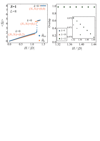
Figure 6: Left panel: Magnetization curves for the two $S=1$ models $\hat{\mathcal{H}}_{DH}$ and $\hat{\mathcal{H}}_{{\rm p}}$. The system size is set at $L=8$. The crystal momentum in the ground state is always zero for both models. The number of solitons $N_{f}$ of heights $f=1,2$ present in the ground state $|{\rm g}_{\rm p}\rangle$ for $\hat{\mathcal{H}}_{{\rm p}}$ is also shown. Right panel: Overlap $|\langle{\rm g}_{\rm p}|{\rm g}_{DH}\rangle|$ between the ground states $|{\rm g}_{\rm p}\rangle,|{\rm g}_{DH}\rangle$ for the two models for the system sizes $L=8$, 10, 12. The magnetic field lies in the range $H/D=1.32-1.44$, where single soliton states of maximal height (=2) dominate the ground state of $\hat{\mathcal{H}}_{DH}$. The inset of the right panel is a blowup of the vertical axis.

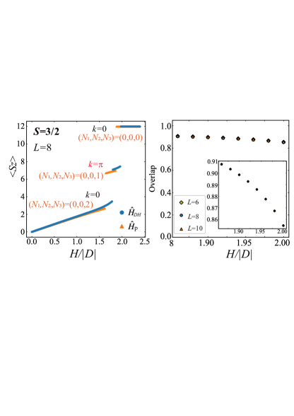
Figure 7: Left panel: Magnetization curves for $S=3/2$ $\hat{\mathcal{H}}_{DH}$ and $\hat{\mathcal{H}}_{{\rm p}}$ for finite-sized systems with $L=8$. The crystal momentum in the ground state changes by $\pm\pi$ accompanying the discontinuous changes in the magnetization. The number of solitons $N_{f}$ of heights $f=1,2$ present in the ground state $|{\rm g}_{\rm p}\rangle$ for $\hat{\mathcal{H}}_{{\rm p}}$ is also shown. Right panel: Overlap $|\langle{\rm g}_{\rm p}|{\rm g}_{DH}\rangle|$ between the ground states $|{\rm g}_{\rm p}\rangle,|{\rm g}_{DH}\rangle$ for the two models for $S=1$ with $L$=8, 10, 12 for the magnetic field in the range of $H/D=1.86-2.00$, where the single soliton states with maximum height (=3 for $S=3/2$) dominate the ground state of $\hat{\mathcal{H}}_{DH}$. The inset of the right panel is a blowup of the vertical axis.

We have confirmed that the overlaps between the ground states for $\hat{\mathcal{H}}_{DH}$ and $\hat{\mathcal{H}}_{{\rm p}}$ slightly below their respective critical fields are larger than 97$\%$ for $S=1$, and larger than 91$\%$ for $S=3/2$.

Having thus seen that it is reasonable for our purpose to work with $\hat{\mathcal{H}}_{{\rm p}}$, we turn to its spectral properties that can be established in a rigorous manner.

V.0.2 Exact results

Theorem 2 (height parity effect)
The lowest energy eigenstate of the p$DH$ Hamiltonian $\hat{\mathcal{H}}_{{\rm p}}$ (Eq. (34)), within the sector where the eigenvalues of the operators $\hat{N}_{1},\hat{N}_{2},\cdots,\hat{N}_{2S}$ are $N_{1},N_{2},\cdots,N_{2S}$, respectively, has the crystal momentum $k=\pi\sum_{f=1}^{2S}fN_{f}$.
As a consequence of this theorem, we find that
Corollary 1 (spin parity effect)
The lowest energy eigenstate of the p$DH$ Hamiltonian $\hat{\mathcal{H}}_{{\rm p}}$, within the sector where the eigenvalues of the operators $\hat{N}_{1},\hat{N}_{2},\cdots,\hat{N}_{2S}$ are $0,0,\cdots,N_{2S}$, respectively, has the crystal momentum $k=2\pi SN_{2S}$.
 
This corollary, encompassing Theorem 1 which is specific to $S=1/2$, and its higher $S$ generalizations, will later be seen to be of direct relevance in understanding the magnetization behavior of the models discussed in this paper. As with Theorem 1, a crucial part of proving Theorem 2 consists in finding a signed basis such that the off-diagonal matrix element of $\hat{\mathcal{H}}_{{\rm p}}$ is non-positive. For that purpose we introduce a unitary operator

$$\hat{U}:=\exp\left[i\pi\sum_{j=1}^{L}\sum_{f=1}^{2S}\sum_{a=0}^{2S-f}jf\hat{P}_{j}^{(S-a)}\hat{P}_{j+1}^{(S-a-f)}\right].$$ (35)

We observe that the projection operator $\hat{P}_{j}^{(S-m)}$ as defined in Eq. (30), and therefore the unitary operator $\hat{U}$ can be expressed solely in terms of {$\hat{S}_{i}^{z}$}. Thus the basis vectors $|\bm{n}\rangle$ are eigenvectors of $\hat{U}$, where it is clear from the definition Eq. (35) that the corresponding eigenvalues are sign factors dependent on $\bm{n}$. One can verify that this dependence can be written explicitly in the following form:

$$\hat{U}|\bm{n}\rangle=(-1)^{\delta(\bm{n})}|\bm{n}\rangle,$$ (36)

where $\delta(\bm{n})$ was defined back in Eq. (13) when dealing with the $S=1/2$ case. We note that the integer $n_{i}$ which appears in Eq. (13) now take the values $\{0,1,2,\cdots,2S\}$. Figure 8 shows examples of $\delta(\bm{n})$ for higher $S$.

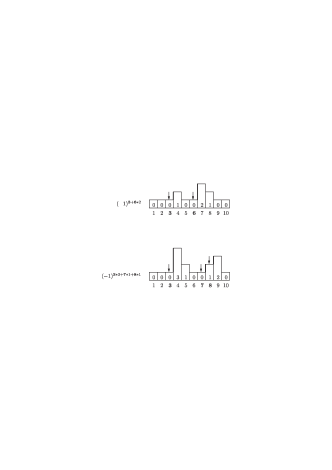
Figure 8: Schematic illustration of the sign $(-1)^{\delta(\bm{n})}$ for $S=1$ (upper panel) and $S=3/2$ (lower panel). The symbol $\delta(\bm{n})$ was defined by Eq. (13).

We also introduce the notation $V(\{N_{f}\})$ as the set of $\bm{n}$ such that $|\bm{n}\rangle$ is a simultaneous eigenvector of $\hat{N}_{1},\cdots,\hat{N}_{2S}$ with eigenvalue $N_{1},\cdots,N_{2S}$. We also denote by $V_{\mu}(\{N_{f}\})$ the subset of $V(\{N_{f}\})$ in which the Hamiltonian $\hat{\mathcal{H}}_{{\rm p}}$ is irreducible. The index $\mu$ runs from 1 to $\sharp(\{V_{\mu}\{N_{f}\}\}_{\mu})$, which is the number of irreducible subspaces in $V(\{N_{f}\})$. We denote the dimension of $V_{\mu}(\{N_{f}\})$ by $d(V_{\mu}(\{N_{f}\})$.

The proof of Theorem 2 relies on the following four Lemmas.  
Lemma 3 (sign of translated basis states)

$$(-1)^{\delta(\bm{n})}=(-1)^{\delta(T(\bm{n}))}(-1)^{\sum_{f=1}^{2S}fN_{f}},$$ (37)

which is a generalization of Eq. (16) to higher $S$.

The proof of Lemma 3 will be given after Lemma 6 is stated.  
Lemma 4 (off-diagonal matrix element)
In the signed basis, the off-diagonal matrix elements are non-positive, i.e.

$$(-1)^{\delta(\bm{n}^{\prime})+\delta(\bm{n})}\langle\bm{n}^{\prime}|\hat{\mathcal{H}}_{{\rm p}}|\bm{n}\rangle\leq 0,$$ (38)

which is a generalization of Lemma 1 to higher $S$.

The proof of Lemma 4 will be given after Lemma 6 is stated.  
Lemma 5 (kernel of $\hat{\mathcal{H}}_{{\rm p}}(H=0)$)
Let us denote by $\hat{\mathcal{H}}_{{\rm p}0}$ the Hamiltonian $\hat{\mathcal{H}}_{{\rm p}}(H=0)$. Among the states in Ker($\hat{\mathcal{H}}_{\rm p0}$), the state $|00\cdots 00\rangle$ has the lowest energy and is a simultaneous eigenstate of $\hat{T}$ and $\hat{N}$ with $k=0$ and $N_{1}=N_{2}=\cdots=N_{2S}=0$.

The proof of Lemma 5 will be given after Lemma 6 is stated.  
Lemma 6 (irreducibility)
When $|\bm{n}\rangle\in V_{\mu}(\{N_{f}\})$ with $d(V_{\mu}(\{N_{f}\}))>1$, $|T(\bm{n})\rangle\in V_{\mu}(\{N_{f}\})$, i.e. there is a positive integer $l$ such that

$$\langle\bm{n}|(\hat{\mathcal{H}}_{{\rm p}})^{l}|T(\bm{n})\rangle\neq 0$$ (39)

We defer the proof of Lemma 6 to the Supplemental Material[30].
 
Proof of Lemma 3

Proof.

We begin by observing that the site-translation operator $\hat{T}$ commutes with $\hat{N}_{f}$ for $f=1,\cdots,2S$ under the periodic boundary condition $\hat{\bm{S}}_{L+1}=\hat{\bm{S}}_{1}$, because the site-translation does not change the numbers and heights (depths) of solitons (valleys). A straightforward calculation shows that $\hat{T}$ is transformed via a unitary operator as

$$\hat{U}\hat{T}=\exp\left(i\pi\sum_{f=1}^{2S}f\hat{N}_{f}\right)\hat{T}\hat{U}.$$ (40)

The derivation of Eq. (40) is deferred to the Supplemental Material[30]. Using the definition of $|T(\bm{n})\rangle$ and taking into account the sign in Eq. (37), we see that

$$\hat{U}\hat{T}|\bm{n}\rangle=(-1)^{\delta(T(\bm{n}))}|T(\bm{n})\rangle$$ (41)

can be rewritten as

$$\hat{U}\hat{T}|\bm{n}\rangle =\exp\left(i\pi\sum_{f=1}^{2S}f\hat{N}_{f}\right)\hat{T}\underbrace{\hat{U}|\bm{n}\rangle}_{(-1)^{\delta(\bm{n})}|\bm{n}\rangle}$$

$$=(-1)^{\delta(\bm{n})}\exp(i\pi\sum_{f=1}^{2S}f\hat{N}_{f})\hat{T}|\bm{n}\rangle$$

$$=(-1)^{\delta(\bm{n})}\hat{T}\exp(i\pi\sum_{f=1}^{2S}f\hat{N}_{f})|\bm{n}\rangle$$

$$=(-1)^{\delta(\bm{n})+\sum_{f=1}^{2S}fN_{f}}\hat{T}|\bm{n}\rangle$$

$$=(-1)^{\delta(\bm{n})+\sum_{f=1}^{2S}fN_{f}}|T(\bm{n})\rangle.$$ (42)

Equating the right-hand side of Eq. (41) with the expression given in the last line of Eq. (42), we arrive at Eq. (37). ∎

Proof of Lemma 4

Proof.

Let us start by recasting the Hamiltonian of Eq. (34) into a form more suitable for the present discussion. Consider restricting the local Hamiltonian to the Hilbert space spanned by $|\bm{n}\rangle$ satisfying

$${\rm min}(n_{i-1},n_{i+1})\leq n_{i}\leq{\rm max}(n_{i-1},n_{i+1}).$$ (43)

The numbers $\{\hat{N}_{f}\}_{f=1}^{2S}$ are then conserved. In contrast, $\hat{h}_{i}$ changes the height of a soliton with a peak at $i$ if ${\rm max}(n_{i-1},n_{i+1})<n_{i}$. Likewise when $n_{i}<{\rm min}(n_{i-1},n_{i+1})$, $\hat{h}_{i}$ changes the depth of its valley whose lowest point resides at site $i$. Introduce a projection operator onto the space satisfying (43) as

$$\hat{\mathcal{P}}_{i}=\sum_{a=0}^{2S}\sum_{b=0}^{2S}\hat{P}_{i-1}^{(S-a)}\hat{P}_{i+1}^{(S-b)}\left(\sum_{k={\rm min}(a,b)}^{{\rm max}(a,b)}\hat{P}_{i}^{(S-k)}\right).$$ (44)

In terms of $\hat{\mathcal{P}}_{i}$, $\hat{\mathcal{H}}_{{\rm p}}$ can be rewritten as

$$\hat{\mathcal{H}}_{{\rm p}}=-H\sum_{i=1}^{L}\hat{S}_{i}^{z}-\frac{D}{2}\sum_{i=1}^{L}\hat{\mathcal{P}}_{i}\hat{h}_{i}\hat{\mathcal{P}}_{i},$$ (45)

where $\hat{h}_{i}$ was defined by Eq. (11). The summand in the second term in the right-hand side is further rewritten as

$$\hat{\mathcal{P}}_{i}\hat{h}_{i}\hat{\mathcal{P}}_{i}=2\sum_{a=0}^{2S}\sum_{b=0}^{2S}(a-b)\hat{\mathcal{S}}_{i}^{x}(a,b)\hat{P}_{i-1}^{(S-a)}\hat{P}_{i+1}^{(S-b)},$$ (46)

with

$$\hat{\mathcal{S}}_{i}^{x}(a,b):=\left(\sum_{k={\rm min}(a,b)}^{{\rm max}(a,b)}\hat{P}_{i}^{(S-k)}\right)\hat{S}_{i}^{x}\left(\sum_{k^{\prime}={\rm min}(a,b)}^{{\rm max}(a,b)}\hat{P}_{i}^{(S-k^{\prime})}\right).$$ (47)

Under the unitary tranformation

$$\hat{\mathcal{H}}_{{\rm p}}^{\prime}:=\hat{U}\hat{\mathcal{H}}_{{\rm p}}\hat{U}^{\dagger},$$ (48)

our Hamiltonian $\hat{\mathcal{H}}_{{\rm p}}$ becomes

$$\hat{\mathcal{H}}_{{\rm p}}^{\prime}=-H\sum_{i=1}^{L}\hat{S}_{i}^{z}-D\sum_{i=1}^{L}\hat{h}^{\prime}_{i},$$ (49)

where

$$\hat{h}^{\prime}_{i} =\sum_{a=0}^{2S}\sum_{b=0}^{2S}(a-b)\hat{U}\hat{\mathcal{S}}_{i}^{x}(a,b)\hat{P}_{i-1}^{(S-a)}\hat{P}_{i+1}^{(S-b)}\hat{U}^{\dagger}$$ (50)

$$=\sum_{a=0}^{2S}\sum_{b=0}^{2S}|a-b|\hat{\mathcal{S}}_{i}^{x}(a,b)\hat{P}_{i-1}^{(S-a)}\hat{P}_{i+1}^{(S-b)}.$$ (51)

Details on how the first line of the above equation, Eq. (50), leads to the second, Eq. (51), is provided in the Supplemental Material[30]. Noting that $\hat{\mathcal{S}}_{i}^{x}(a,b)$ is the product of projection operators and $\hat{S}_{i}^{x}$ leads to

$$\langle\bm{n}^{\prime}|\hat{\mathcal{H}}^{\prime}_{{\rm p}}|\bm{n}\rangle\leq 0,\quad\mbox{ for }\bm{n}\neq\bm{n}^{\prime}.$$ (52)

Using this relation, we find that

$$(-1)^{\delta(\bm{n}^{\prime})+\delta(\bm{n})}\langle\bm{n}^{\prime}|\hat{\mathcal{H}}_{{\rm p}}|\bm{n}\rangle$$

$$=\langle\bm{n}^{\prime}|\hat{U}\hat{\mathcal{H}}_{{\rm p}}\hat{U}^{\dagger}|\bm{n}\rangle$$

$$=\langle\bm{n}^{\prime}|\hat{\mathcal{H}}^{\prime}_{{\rm p}}|\bm{n}\rangle\leq 0.$$ (53)

∎

Proof of Lemma 5

Proof.

The set of the states $|\bm{n}\rangle\in V_{\mu}(\{N_{f}\})$ with $d(V_{\mu}(\{N_{f}\}))=1$ forms the basis of Ker($\hat{\mathcal{H}}_{\rm p0}$). Each basis vector $|\bm{n}\rangle$ is an eigenstate of the Zeeman energy. The fully polarized state $|00\cdots 00\rangle$ has the lowest Zeeman energy and thus is the lowest energy state in Ker($\hat{\mathcal{H}}_{\rm p0}$). ∎

Proof of Theorem 2
This proof is similar to that for Theorem 1, and proceeds by replacing $(-1)^{N}$ by $(-1)^{\sum_{f=1}^{2S}fN_{f}}$ in Eqs. (16), (25), and (26) .

Proof.

When the ground state is given by $|00\cdots 00\rangle$, theorem 2 holds (Lemma 5). According to Lemma 5, other $|{\bm{n}}\rangle$s belonging to $V_{\mu}(\{N_{f}\})$ with $d(V_{\mu}(\{N_{f}\}))=1$ cannot be the ground state. We thus focus on the case where the ground state is spanned by $|{\bm{n}}\rangle$ with ${\bm{n}}$ belonging to $V_{\mu}(\{N_{f}\})$ for which $d(V_{\mu}(\{N_{f}\}))>1$.

When $N_{f}\neq 0$ for a certain $f$, it follows from Lemmas 4 and 6 and the Perron-Frobenius theorem[31] that the lowest energy eigenstate of $\hat{\mathcal{H}}_{{\rm p}}$ for each eigenspace consisting of $\bm{n}\in V_{\mu}(\{N_{f}\})$ is non-degenerate and the state vector $|E_{{\rm min},\{N_{f}\},\mu}\rangle$ is spanned by the signed basis where all coefficients are positive, i.e.,

$$|E_{{\rm min},\{N_{f}\},\mu}\rangle= \sum_{\bm{n}\in V_{\mu}(\{N_{f}\})}a(\bm{n})(-1)^{\delta(\bm{n})}|\bm{n}\rangle,$$ (54)

with $a(\bm{n})>0$. From the nondegeneracy of $|E_{{\rm min},N}\rangle$, it is an eigenstate of the site-translation operator $\hat{T}$ and thus

$$|a(\bm{n})|=|a(T(\bm{n}))|,$$ (55)

which leads to $a(\bm{n})=a(T(\bm{n}))$ because $a(^{\forall}\bm{n}\in V_{N})>0$. We can thus rewrite Eq. (54) as

$$|E_{{\rm min},\{N_{f}\},\mu}\rangle$$

$$= a(\bm{n})\left((-1)^{\delta(\bm{n})}|\bm{n}\rangle+(-1)^{\delta(T(\bm{n}))}|T(\bm{n})\rangle+\cdots\right)$$

$$+\cdots$$ (56)

$$= a(\bm{n})(-1)^{\delta(\bm{n})}\left(|\bm{n}\rangle+(-1)^{\sum_{f=1}^{2S}fN_{f}}|T(\bm{n})\rangle+\cdots\right)$$

$$+\cdots.$$ (57)

This implies that

$$\hat{T}|E_{{\rm min},\{N_{f}\},\mu}\rangle=(-1)^{\sum_{f=1}^{2S}fN_{f}}|E_{{\rm min},\{N_{f}\},\mu}\rangle.$$ (58)

∎

VI Chirality of Quantum Solitons

Up to now we have not explicitly addressed the role that chirality plays in our problem. Let us define the chirality of a state by

$$\mbox{ch}=\langle\sum_{j}\left(\hat{\bm{S}}_{j}\times\hat{\bm{S}}_{j+1}\right)_{y}\rangle=\frac{1}{D}\langle\hat{\mathcal{H}}_{\rm DM}\rangle$$ (59)

in analogy with [32]. We can then readily show

$$\mbox{ch}<0,\quad\mbox{when } D>0$$ (60a)

$$\mbox{ch}>0,\quad\mbox{when } D<0$$ (60b)

to be true in the lowest energy state in any given irreducible space $V_{\mu}(\{N_{f}\})$ with $d_{\mu}(\{N_{f}\})\neq 1$. To establish Eq. (60a), we observe that

$$\mbox{ch}= \frac{1}{D}\langle E_{{\rm min},\{N_{f}\},\mu}|\hat{\mathcal{H}}_{\rm DM}|E_{{\rm min},\{N_{f}\},\mu}\rangle$$

$$= \frac{1}{D}\sum_{\bm{n},\bm{n}^{\prime}\in V_{\mu}(\{N_{f}\})}\underbrace{\langle\bm{n}|\hat{\mathcal{H}}_{\rm DM}|\bm{n}^{\prime}\rangle(-1)^{\delta(\bm{n})+\delta(\bm{n}^{\prime})}}_{<0}\underbrace{a(\bm{n})a(\bm{n}^{\prime})}_{>0}$$

$$<0,$$ (61)

with the use of Eq. (22) and theorem 2. Equation (60b) can likewise be verified. In the previous sections, we have always assumed that $D>0$. Taking the choice $D<0$ require us to replace $\delta(\bm{n})$ with

$$\delta^{(-)}(\bm{n})=\sum_{j=1}j(n_{L-j}-n_{L+1-j}+|n_{L-j}-n_{L+1-j}|)/2$$ (62)

and Eq. (22) with

$$|E_{{\rm min},N}\rangle= \sum_{\bm{n}\in V_{N}}a(\bm{n})(-1)^{\delta^{(-)}(\bm{n})}|\bm{n}\rangle.$$ (63)

Equation (62) is obtained by replacing $n_{j}$ with $n_{L+1-j}$ in Eq. (13). Examples of the signed basis for $D<0$ are shown in Fig. 9.

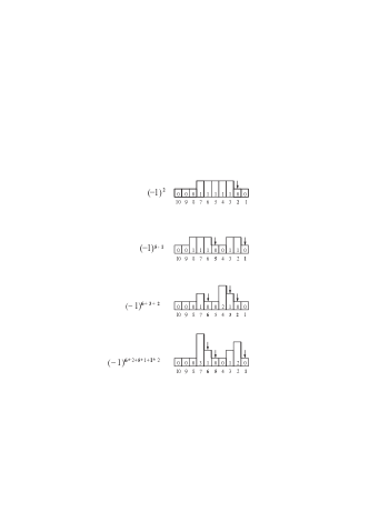
Figure 9: Examples of signed basis for negative $D$. The upper two panels represent basis states for $S=1/2$ corresponding to those shown in Fig. 4. The sign $(-1)^{\delta^{(-)}(\bm{n})}$ uses $\delta^{(-)}(\bm{n})$ defined in Eq. (63). The lower two panels represent basis states for $S=1$ and $S=3/2$, which correspond to the figures shown in Fig. 8. The numbers underneath the figures represent $L-j$ where $j$ is the site index.

VII Effect of exchange interactions

Among the exchange interactions in $\hat{\mathcal{H}}_{\rm ch}$, the presence of the Ising term $-J\sum_{i}\hat{S}_{i}^{z}\hat{S}_{i+1}^{z}$ is immaterial to our argument in the previous section in the sense that it commutes with $\hat{N}$ and it is diagonal in the basis $\{|\bm{n}\rangle\}$. The XY term $-J\sum_{i}(\hat{S}_{i}^{x}\hat{S}_{i+1}^{x}+\hat{S}_{i}^{y}\hat{S}_{i+1}^{y})=\hat{\mathcal{H}}_{\rm XY}$, in contrast, does not conserve $\hat{N}$, e.g.,

$$\hat{\mathcal{H}}_{\rm XY}|011100\rangle=-\frac{J}{2}\left(|101100\rangle+|011010\rangle\right),$$ (64)

for $S=1/2$. Equation (64) represents the matrix elements between $N=1$ and $N=2$. The ground state of $\hat{\mathcal{H}}_{\rm ch}$ is thus given by a linear combination of states with different numbers of solitons.

We examine numerically to what extent the single soliton basis (the set of eigenstate of $\hat{N}$ with $N=1$) accounts for the ground state wavefunction of $\hat{\mathcal{H}}_{\rm ch}$. We set $J=D$. Slightly below the critical field, and for site numbers up to $L=20$ for $S=1/2$ ($L=16$ for $S=1$), we find that 80 (58) percent of the weight of the exact ground state $|{\rm g}\rangle$ of $\hat{\mathcal{H}}_{\rm ch}$ is made up of states belonging to the single soliton basis. Details of this examination is shown in Fig. 10, where for the $S=1/2$ case, the weight of the one-soliton state within the ground state of $\hat{\mathcal{H}}_{\rm ch}$, i.e. $\langle{\rm g}|\hat{P}(N_{1}=1)|{\rm g}\rangle$ is displayed as a function of $1/L$ in the left panel. Likewise, for $S=1$ (right panel), we have evaluated the corresponding weight $\langle{\rm g}|\hat{P}(N_{1}=0,N_{2}=1)|{\rm g}\rangle$. We take these results to be a strong indication that the physical picture derived rigorously in the $J=0$ limit continues to be valid qualitatively even when $J$ is comparable to $D$.

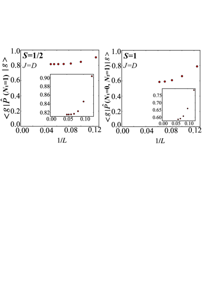
Figure 10: Size dependence of the weight of the one-soliton states in the ground state of $\hat{\mathcal{H}}_{\rm ch}$ for $J=D$ and $S=1/2$ (left panel) and $S=1$ (right panel). The magnetic field is set at $H/D=0.29$ ($H/D=0.5$) for $S=1/2$ ($S=1$). The insets of both panels magnify the vertical axis.

VIII Discussions

In the preceding, we established that in the p$DH$ models for arbitrary $S$, a soliton whose height is $f$ has a crystal momentum of $\pi f$ in its lowest energy state. More generally, we verified in a rigorous manner that the lowest energy state belonging to the sector $(N_{1},\cdots,N_{2S})$, where $N_{f}(1\leq f\leq 2S)$ is the number of solitons of amplitude $f$ present in this state, has the crystal momentum $k=\pi\sum_{f}fN_{f}$. We have termed our finding the height parity effect. To demonstrate the power of this result, we note that it immediately rules out a spin parity effect for a spin wave, which is identified with a soliton of height $f=1$ and length $1$: the crystal momentum of this state is $k=\pi$ irrespective of the value of $S$.

Numerical calculations show that only solitons with the maximal height $f=2S$ contribute to the ground state of the p$DH$ model. This implies that the height parity effect for the ground state of this model is $k=2\pi SN_{2S}$, which is precisely the observed spin parity effect.

The magnetization processes of the p$DH$ models for each $S$ consist of successive level crossings from a $N_{2S}$-soliton state to a $N_{2S}-1$-soliton state. For half-integer $S$, each level crossing is protected by the soliton number (which changes by $\Delta N_{2S}=-1$) and the crystal momentum (which changes by $\Delta k=\pi$) while it is protected only by the soliton number for integer $S$. Switching on the exchange interaction, the soliton numbers are no longer conserved quantities and thus the level crossing for integer $S$ turns into a crossover, while it remains protected by a $\pi$-shift in the momentum for half-integer $S$ up to a certain magnitude of exchange interaction $J$. Although this threshold value of $J$ is unknown, our numerical results for magnetization curves and the relative weight of one-soliton state in the ground state for $S=1/2$ and $S=1$ implies that the spin parity effect in monoaxial chiral magnets with $J/D\leq 1$ is well captured by the properties of quantum solitons developed in the present study.

We should caution the reader, though that determining whether a spin parity effect is present as well in monoaxial chiral magnets with a small $S$ and $J\gg D$ as is typical in existing magnets, will require further investigations. If such an effect is indeed verified in systems belonging to the “solid state” limit $J\gg D$, it is premature with the information at hand to claim that its underlying mechanism, along with the proper characterization and definition of a quantum soliton, is the same as those described in this paper, which are valid under the condition $J\leq D$.

That said, it is nevertheless interesting to compare notes with the semiclassical approach, which is considered to work at large $S$ and in the wide-soliton regime $J>D$. This method is described in some detail in Appendix A. The salient points are (1) the recovery of the spin parity effect $k=2\pi S$, and (2) a gauge structure inherent to the effective action which can be viewed as roughly corresponding to the signed basis argument of the main text. While these analogies certainly appear to point to universal aspects which arise for deeper topological reasons that hold irrespective of the specific regime of interest, a firmer understanding on this point remains to be established.

Experimental realizations of the limit $D\gg J$ in non-solid state settings is another direction worth pursuing. In particular, the $S=1/2$ $DH$ model, if realized will serve as an ideal platform for studying the quantum dynamics of solitons. On this front we mention that a proposal has recently been made to realize a system equivalent to this model using Rydberg atoms [33].

Among other apparently significant issues that remain, is a thorough investigation into possible spin parity effects for general $S$ from a purely quantum approach for the following systems: antiferromagnetic chiral magnets in 1d[34] and 2d, 2d chiral ferromagnets accommodating skyrmions [22, 35], and non-chiral magnets with stable solitons arising from an Ising anisotropy[19]. We hope that the present work will inspire activities in this direction that will go a long way toward painting a coherent picture for spin parity effects in quantum magnets.

IX Summary

In summary, we have numerically verified and subsequently tracked down the mechanism responsible for a spin parity effect which is present in the ground state of a monoaxial chiral ferromagnet spin chain.

Our study started with a numerical evaluation of the magnetization curve for finite sized systems falling within the regime $J\leq D$. For half-odd integer $S$, the curve consists of level crossings accompanied by a jump of the crystal momentum by the amount $\pi$. The behavior is very different when $S$ is integral: the curve is continuous, features crossover events, and the ground state’s crystal momentum remains zero throughout.

To get a handle on this problem, we constructed a limiting-case Hamiltonian, the $S=1/2$ $DH$ model, where the soliton number is a conserved quantity. We established rigorously that the lowest-energy state with $N$ solitons has the crystal momentum $\pi N$.

Encouraged by this result, we constructed a natural generalization of the $DH$ model to arbitrary $S$, the p$DH$ model (which reduces to the former when $S=1/2$). Quantum solitons in the $S_{z}$ basis, of integer-valued heights ranging from 1 to $2S$, are all conserved quantities of this model. Let $N_{f}$ be the numbers of height-$f$ solitons that are present in a given state. We showed rigorously that the lowest energy state within the sector $(N_{1},\cdots,N_{2S})$ possesses the crystal momentum $\pi\sum_{f}fN_{f}$ (the height parity effect). The spin parity effect $k=2\pi SN_{2S}$, which is realized in the ground state of this model follows from the height parity effect when all $N_{f}$s are zero with the sole exception of $N_{2S}$.

The p$DH$ model thus allows for an interpretation of the spin parity effect which governs its magnetization process in terms of sharply-defined quantum solitons. It also serves to provide a physical picture for the same effect which is observed in the more general model of a monoaxial chiral ferromagnet with a finite $J$ when $J/D\leq 1$. We have confirmed numerically that the picture derived from the p$DH$ model holds up in this regime.

Appendix A The semiclassical approach

In this appendix we record for completeness what a semiclassical treatment using the spin coherent state path integral, which is valid at large $S$ and under the condition $J>D$, says about the quantum mechanical features of solitons that we have discussed in the main text. Much of what follows borrows heavily from the work of Braun and Loss[19] on the quantum dynamics of solitons in nonchiral magnets. Differences that arise in the chiral counterpart will be highlighted as they appear. As mentioned in the main text (see the Discussion section), it must be stressed that extrapolating the results of a semiclassical analysis to the regime relevant to the present paper is not straightforward. Still the reader will notice interesting parallels between the two approaches, which we believe is well worth appreciating.

A.1 Long wavelength effective action

We take up the same Hamiltonian as in the main text:

$${\cal H} = -J\sum_{\langle ij\rangle}{\bm{S}}_{i}\cdot{\bm{S}}_{j}-h\sum_{j}S_{j}^{z}+K\sum_{j}\left(S_{j}^{y}\right)^{2}$$ (65)

$$-\sum_{\langle ij\rangle}D{\hat{y}}\cdot{\bm{S}}_{i}\times{\bm{S}}_{j}.$$

where $J,K>0$. In this appendix we will choose to align the spin chain with the $y$-axis.

In the following we will work in Euclidean space-time and put $\hbar=1$. The spin coherent state path integral approach then consists of writing each spin vector as c-numbered entities ${\bm{S}}_{j}=S{\bm{n}}_{j}$ where ${\bm{n}}_{j}^{2}=1$, and studying the action

$${\cal S}[\{{\bm{n}}_{j}(\tau,x)\}]={\cal S}_{\rm BP}+\int d\tau{\cal H}.$$ (66)

The first term ${\cal S}_{\rm BP}$ records the spin Berry phase, i.e.

$${\cal S}_{\rm BP} = \sum_{j}iS\omega[{\bm{n}}_{j}(\tau)]$$ (67)

$$= \sum_{j}iS(1-\cos\theta_{j}(\tau))\partial_{\tau}\phi_{j}(\tau),$$

where $\omega[{\bm{n}}_{j}(\tau)]$ is the solid angle traced out on the unit sphere by the vector ${\bm{n}}_{j}(\tau)$ in the course of its imaginary-time evolution. In the second line we have introduced the spherical coordinates $(\theta,\phi)$ via

$$n_{x}=\sin\theta\sin\phi,n_{y}=\cos\theta,n_{z}=\sin\theta\cos\phi.$$

Below we take the continuum limit and seek the low energy effective action for our system. Assume that $K\gg J$. Since we then expect $n_{y}(\tau,y)$, the hard-axis component of ${\bm{n}}$ to be sufficiently small compared to the portion lying within the easy ($zx$-)plane, it suffices to employ the parametrization $\theta=\pi/2-\delta\theta$, and ignore the periodic nature of the angular variable $\delta\theta$. The $2\pi$-periodicity of $\phi$, on the other hand is essential for keeping track of solitons and will be retained. We now expand each term in the Hamiltonian ${\cal H}$ up to quadratic order in $\delta\theta$.

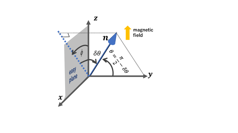
Figure 11: Spherical coordinate and geometry used in the text.

Collecting $\delta\theta$-related contributions, we have

$${\cal L}_{\delta\theta}=\frac{KS^{2}}{a}(\delta\theta)^{2}+\frac{JS^{2}}{2a}(\partial_{y}\delta\theta)^{2}-i\frac{S}{a}(\partial_{\tau}\phi)\delta\theta.$$

The notation $a$ stands for the lattice constant. The last term on the right comes from the Berry phase action ${\cal S}_{\rm BP}$. Focusing on the long wavelength regime where only Fourier modes satisfying $k_{y}\ll 1\ll\sqrt{\frac{K}{J}}$ are incorporated, we can readily integrate over the $\delta\theta$ fluctuations in ${\cal L}_{\delta\theta}$, which leaves us with a new term $\frac{S}{4Ka}(\partial_{\tau}\phi)^{2}$. (Physically this can be understood by noting that since, from (67), $n_{y}$ is canonically conjugate to $\phi$, the hard axis anisotropy term $\sim n_{y}^{2}$ can be traded for the kinetic energy related to the dynamics of $\phi$, i.e. $\sim{\dot{\phi}}^{2}$. ) On combining with the remaining terms, we arrive at an effective action ${\cal S}_{\rm eff}[\phi(\tau,x)]=\int d\tau dx{\cal L}_{\rm eff}$, where

$${\cal L}_{\rm eff} = i\frac{S}{a}\partial_{\tau}\phi+\frac{JS^{2}}{2a}\left[\frac{1}{{c_{s}}^{2}}(\partial_{\tau}\phi)^{2}+(\partial_{y}\phi)^{2}\right]$$ (68)

$$-\frac{DS^{2}}{a}\partial_{y}\phi-\frac{hS}{a^{2}}\cos\phi,$$

and $c_{s}=\sqrt{KJSa}$. This is a chiral variant of the quantum sine-Gordon action. As we will shortly see, the first entry on the right hand side, descending from ${\cal S}_{\rm BP}$, is a topological term which is ultimately responsible for the occurrence of the spin parity effect of soliton excitations as viewed in this semiclassical language.

A.2 Soliton collective coordinates

We proceed to extract from (68) information pertaining to the soliton dynamics. We will focus for simplicity on the one-soliton sector, though similar analysis carries through for more complex situations. We begin by observing that the Euler-Lagrange equation which follows from ${\cal S}_{\rm eff}$ is the quantum sine-Gordon equation

$$\frac{1}{c_{s}^{2}}\phi_{\tau\tau}-\phi_{yy}=M^{2}\sin\phi,\hskip 8.53581ptM^{2}=\frac{h}{JSa},$$ (69)

where subscripts stand for derivatives. Static soliton and antisoliton solutions of height $2\pi$ can be written explicitly as

$$\phi_{0}(y)=\pm 4\tan^{-1}e^{M(y-Y)},$$ (70)

as can easily be verified by direct inspection. The letter $Y$ in the above stands for the center coordinate of the soliton. While the DM term, being a total derivative, does not enter into the equation of motion (69), it plays the important role of selecting out the energetically favorable sign in (70), which in the present convention is positive. (One needs to incorporate it explicitly though when incommensurability effects set in at lower magnetic fields.)

We are now ready to promote the soliton’s position $Y$ to a dynamical collective coordinate $Y(\tau)$. Plugging the configuration $\phi_{0}(y-Y(\tau))$ into (68), we find

$${\cal S}_{Y}[Y(\tau)]=\int d\tau\left[-i\frac{2\pi S}{a}\dot{Y}+\frac{1}{2\tilde{M}}\dot{Y}^{2}\right],$$ (71)

where ${\tilde{M}}=\frac{a}{8JS^{2}M}$. Here we have assumed a soliton of height $2\pi$, or equivalently a configuration for which the winding number $Q\equiv\frac{1}{2\pi}\int_{-\infty}^{\infty}dy\partial_{y}\phi_{0}$ is unity. The generalization to arbitrary $Q$ is straightforward, where, in particular the first term on the right is simply multiplied by that integer. This is formally equivalent to the action of a charged point particle, with the first term representing the coupling between the particle and a (Berry) gauge field. We will see in a moment that this coupling term, despite it being a total derivative, is absolutely crucial for arriving at the correct quantum mechanical features.

It is natural to expect that the soliton, now viewed as a quantum mechanical particle hopping through the spin chain, also experiences an effective periodic potential $V(y)$ with the property $V(y+a)=V(y)$, which imprints the underlying lattice structure on the dynamics and thus renders the soliton to form Bloch bands. We refer the reader to Braun and Loss[19] for an explicit evaluation of this potential, which can be carried out e.g. by treating inter-site tunneling events in a instanton gas approximation. The corresponding Hamiltonian which takes these three terms into account is

$${\cal H}=\frac{1}{\tilde{M}}({\hat{P}}_{Y}-\frac{2\pi S}{a})^{2}+V(Y),$$ (72)

with ${\hat{P}}_{Y}$ the momentum operator conjugate to $Y$. It is clear from this form that the lowest energy state in the 1-soliton sector carries a crystal momentum of $p_{\rm sol}=\frac{2\pi S}{a}$, reproducing the findings of the main text.

Having seen how the spin Berry phase has made its way into the expression for $p_{\rm sol}$, it is instructive to perform at this point a sanity check: recall that for the Berry phase action (67) we made use of the so-called north-pole gauge, in which the Dirac string goes through the south pole. We could have equally well opted to use the south-pole gauge, where ${\cal S}_{\rm BP}=\sum_{j}iS(-1-\cos\theta_{j}(\tau))\partial_{\tau}\phi_{j}(\tau)$. Repeating the whole procedure for the latter, we find that the value of $p_{\rm sol}$ merely shifts by $\frac{2\pi}{a}$, thereby demonstrating the gauge independence of the result. The lesson to be learned then, as emphasized early on by Haldane[37], is that retaining the full expression for the solid angle $\omega$ (whatever choice of gauge one makes) is crucial for safely extracting information on the crystal momenta of a ferromagnet.

As a final note before proceeding, we remark that we could have foreseen the value of the crystal momentum determined in this subsection, once we have chosen to focus on a $2\pi$ soliton: we adopt for this purpose Haldane’s semiclassical theory[37] mentioned above, which states that if a snapshot configuration ${\bm{n}}(y)$ of a 1d ferrromagnet obeying a periodic boundary condition subtends a solid angle $\omega[{\bm{n}}(y)]$, that state carries the crystal momentum $\frac{S}{a}\omega$. As $\omega=2\pi$ for a $2\pi$ soliton, this relation reproduces the result $p_{\rm sol}=\frac{2\pi S}{a}$. (We should also mention that the identification of the crystal momentum of a soliton in its lowest energy state, with the Berry phase associated with the snapshot spin configuration appears in several of the earlier work on chiral ferromagnetic spin chains[14, 38, 39]. Implications to spin parity effects or to the magnetization process, however, are not considered there.)

A.3 Effect of magnetic fluctuations

The foregoing basically followed from a treatment at the saddle point level, and as such needs to be submitted to a stability analysis against quantum fluctuations, i.e. the effects of spin wave fluctuations $\varphi$ around the moving rigid-soliton configuration $\phi_{0}$ :

$$\phi(\tau,y)=\phi_{0}(y-Y(\tau))+\varphi(y-Y(\tau),\tau).$$ (73)

As this is not directly related to the spin parity effect, we once again refer the interested reader to Braun and Loss[19, 40] for the relevant technical details, and merely state the outcomes of this analysis. (An alternative method based on Dirac’s formalism for constrained quantum theory can be found in the review article of Kishine and Ovchinikov[14].) An expansion to second order in the spin wave fluctuation yields the spin wave dispersion

$$\epsilon_{k}=\frac{JS^{2}}{2a}(k^{2}+M^{2}),$$ (74)

where one sees that a mass has been induced by the Zeeman field. Meanwhile a coupling between soliton coordinate $Y$ and the spin wave $\varphi$ enters the action at the same order, which can lead to damping (memory) effects as well as a renormalization of the soliton’s rest mass. The former is found to have a characteristic decay time $\tau=\frac{1}{2{\sqrt{Kh}}}$ which, if sufficiently smaller than the time scale on which ${\dot{Y}}$ changes, is negligible. The latter is of the order of ${\cal O}(1/S)$, which in the semi-classical regime should also be small.

A.4 Implications

A remark on the behavior of the magnetization curve in light of the semiclassical effective theory is in order. The Hamiltonian (72) implies that the introduction of an additional $2\pi$ kink into the system, i.e. a process for which $\delta Q=1$, is accompanied by a change in the crystal momentum by the amount

$$\delta P_{Y}=\frac{2\pi S}{a}\delta Q=2\pi S.$$

Thus for half-integer $S$, momentum conservation prohibits tunneling between configurations differing in $Q$ by one. This will result in level crossing. In contrast to this, tunneling and hence level repulsion can occur when $S$ is integral. The same conclusion also follows from a path integral point of view. The kink insertion is a singular space-time process (a phase-slip). Consider two different space-time patterns in which such events occur, the second one centered at a plaquette (in the $y$ vs $\tau$ plane) immediately to the right of the first. These two events each enter the path integral with Feynman weights $e^{-{\cal S}_{\rm Event1}}$ and $e^{-{\cal S}_{\rm Event2}}$, differing only by the phase $e^{-i2\pi S}$, and thereby canceling out when $S$ is half-integral. Since such pair-wise cancellation occurs generically, one concludes that phase slips do not contribute to the partition function.

The spin Berry phase’s influence on soliton dynamics can be modulated by the addition of a longitudinal component (i.e. along the chain) to the external magnetic field[19, 39]. For the problem at hand, this will have the effect of continuously changing the crystal momentum in proportion to the superimposed field. At special values of the latter (ideally there are $2S+1$ such values), the magnetization process in the half-odd integer $S$ case (as a function of the transverse field) is expected to mimic the behavior of an integer $S$ spin chain in the absence of the longitudinal field. The manner in which the spin parity effect is in principle controllable using an external parameter is reminiscent of what happens in antiferromagnetic chains, when one introduces (and continuously varies the strength of) a bond-alternating component to the nearest neighbor exchange interaction [41, 42].

Finally we recall that recognizing the global structure inherent to the ground state wavefunction was the key that lead us to some of the central conclusions of the main text. This prompts us to briefly recapitulate the discussions of the preceding paragraphs from the vantage point of wave function properties. To this end we note that it is possible to envisage a continuum counterpart [43] for the “signed basis” expansion of the ground state’s state vector that was discussed in the main text:

$$|\Psi\rangle = \int{\cal D}\phi(y)e^{-iS\int\frac{dy}{a}\phi(y)}|\phi(y)\rangle\langle\phi(y)|\Psi\rangle$$ (75)

$$\equiv \int{\cal D}\phi(y)e^{-iS\int\frac{dy}{a}\phi(y)}\Psi[\phi(y)]|\phi(y)\rangle.$$

The phase factor $e^{-iS\int\frac{dy}{a}\phi(y)}$ is the continuum analog of the all-important kink-counting sign factor $(-1)^{2S\sum_{\rm kink}j_{\rm kink}}$, where $j_{\rm kink}$ is the lattice site at the left end of a soliton. (The analogy becomes more transparent upon rewriting this factor as $e^{iS\int\frac{dy}{a}y\phi^{\prime}(y)}$.) Meanwhile the wave functional $\Psi[\phi(y)]$ corresponds to the positive-sign expansion coefficients, and should have the property that it can be choosen to be real and nodeless, and exhibit the lattice periodicity $\Psi[\phi(y+a)]=\Psi[\phi(y)]$. The crystal momentum associated with this state can then be obtained as follows. Writing the generator of a one site translation as ${\hat{T}}$, and in addition defining

$${\tilde{\Psi}}[\phi(y)]\equiv e^{-iS\int\frac{dy}{a}\phi(y)}\Psi[\phi(y)],$$ (76)

we have

$${\hat{T}}{\tilde{\Psi}}[\phi(y)] = {\tilde{\Psi}}[\phi(y-a)]$$

$$= {\tilde{\Psi}}[\phi(y)]\times e^{iS\int\frac{dy}{a}\{\phi(y)-\phi(y-a)\}}$$

$$\simeq {\tilde{\Psi}}[\phi(y)]\times e^{iS\int dy(\partial_{y}\phi)}$$

$$= {\tilde{\Psi}}[\phi(y)]\times e^{i2\pi SN}{\hskip 8.53581pt}N:{\rm soliton}{\hskip 4.2679pt}{\rm number}.$$

The resemblance with how the lattice wave function transforms under translation is apparent. To see how this relates to the semiclassical theory (68), we first write down its Hamiltonian for the case where the topological term is absent. This reads

$${\cal H}_{\rm eff} = \int dy\left[\frac{a^{2}K}{S}{\hat{\pi}}_{\phi}^{2}+\frac{JS^{2}}{2a}(\partial_{y}\phi)^{2}\right.$$ (77)

$$\left.{\hskip 22.76219pt}-\frac{DS^{2}}{a}\partial_{y}\phi-\frac{hS}{a^{2}}\cos\phi\right].$$

Here we have used the notation ${\hat{\pi}}_{\phi}(y)\equiv-i\frac{\delta}{\delta\phi(y)}$. Let us call the ground state wave functional for this Hamiltonian $\Psi[\phi(x)]$. As there are no topological terms which act on the solitons as Aharonov-Bohm like fluxes, we expect that $\Psi[\phi(x)]$ can to chosen to be real, is nodeless, and respects the lattice translation symmetry[44]. Upon reintroducing the topological term, the momentum ${\hat{\pi}}_{\phi}$ entering the first term on the right hand side of the above equation receives the shift ${\hat{\pi}}_{\phi}\rightarrow{\hat{\pi}}_{\phi}+\frac{S}{a}$. Since this shift is of the form of a coupling of a charged matter to a gauge field, it is straightforward to see that the wave functional accordingly “gauge transforms” into $e^{-iS\int\frac{dy}{a}\phi(y)}\Psi[\phi(y)]$. The same conclusion is reached by formally expressing the ground state wave functional as a constrained path integral, i.e.$\Psi[\phi(y)]\propto\int{\cal D}\phi(\tau,y)e^{-{\cal S}_{\rm eff}[\phi]}$, where one takes the sum over paths in Euclidean space-time such that the configuration at the terminal imaginary time (which is taken to be sufficiently large) always ends up as $\phi[y]$. In this approach the phase factor $e^{-iS\int\frac{dy}{a}\phi(y)}$ derives from a boundary contribution of the topological term which is generated at the end of the imaginary time axis. (This method is valid provided there is an energy gap between a unique ground state and the excited states.) [45, 46].

To seek the counterpart of the height parity effect and the $DH$ and p$DH$ models in the semiclassical/field-theoretical framework, as well as to undertake a quest for spin parity effects at much lower magnetic fields where incommensurability effects need to be incorporated, are interesting problems that we leave for the future.

S1 Proof of Lemma 2

We denote the relation between $\bm{n}$ and $\bm{n}^{\prime}$ that belong to $V_{N}$ with $N\in[1,L/2-1]$ by $\bm{n}\sim\bm{n}^{\prime}$ when there exists a positive integer $l$ such that

$$M(\bm{n},\bm{n}^{\prime};l)>0,$$ (S1)

with

$$M(\bm{n},\bm{n}^{\prime};l):=(-1)^{\delta(\bm{n})+\delta(\bm{n}^{\prime})}\langle\bm{n}|(-\hat{\mathcal{H}}_{\rm DM})^{l}|\bm{n}^{\prime}\rangle.$$ (S2)

We prove that $\bm{n}\sim\bm{n}^{\prime}$ for arbitrary pairs of $\bm{n}$ and $\bm{n}^{\prime}$ belonging to $V_{N}$ with $N\in[1,L/2-1]$. The off-diagonal matrix elements of $\hat{\mathcal{H}}_{DH}$ in this basis stem from $\hat{\mathcal{H}}_{\rm DM}$. Let the minimum $l$ satisfying Eq. (S1) be $l_{0}$. Then

$$(-1)^{\delta(\bm{n})+\delta(\bm{n}^{\prime})}\langle\bm{n}|(-\hat{\mathcal{H}}_{DH})^{l_{0}}|\bm{n}^{\prime}\rangle=M(\bm{n},\bm{n}^{\prime};l_{0})>0$$ (S3)

follows.  
Lemma S1
The relation $\sim$ is transitive and symmetric.

Proof.

(symmetric) $\bm{n}\sim\bm{n}^{\prime}\leftrightarrow\bm{n}^{\prime}\sim\bm{n}$ because matrix elements of $\hat{\mathcal{H}}_{\rm DM}$ in the present basis is real.
(transitive) When $\bm{n}_{\rm I}\sim\bm{n}_{\rm II}$ and $\bm{n}_{\rm II}\sim\bm{n}_{\rm III}$ for $\bm{n}_{\rm I},\bm{n}_{\rm II},\bm{n}_{\rm III}\in V_{N}$ with $N\in[1,L/2-1]$, there exist positive integers $l_{1}$ and $l_{2}$ such that

$$M(\bm{n}_{\rm I},\bm{n}_{\rm II};l_{1})>0,\quad M(\bm{n}_{\rm II},\bm{n}_{\rm III};l_{2})>0.$$ (S4)

It then follows that

$$M(\bm{n}_{\rm I},\bm{n}_{\rm III};l_{1}+l_{2})$$

$$= \sum_{\bm{n}^{\prime}\in V_{N}}M(\bm{n}_{\rm I},\bm{n}^{\prime};l_{1})M(\bm{n}^{\prime},\bm{n}_{\rm III};l_{2})$$ (S5)

$$= \underbrace{M(\bm{n}_{\rm I},\bm{n}_{\rm II};l_{1})}_{>0}\underbrace{M(\bm{n}_{\rm II},\bm{n}_{\rm III};l_{2})}_{>0}$$

$$+\sum_{\bm{n}^{\prime}(\neq\bm{n}_{\rm II})\in V_{N}}\underbrace{M(\bm{n}_{\rm I},\bm{n}^{\prime};l_{1})}_{\geq 0}\underbrace{M(\bm{n}^{\prime},\bm{n}_{\rm III};l_{2})}_{\geq 0}$$ (S6)

$$>0.$$ (S7)

∎

For a given $\bm{n}$, let $B=B(\bm{n})$ be the set of $i$ such that $n_{i-1}\neq n_{i}$. We label these elements $B(\bm{n})=\{b_{\alpha}\}$ in the increasing order

$$1\leq b_{1}<b_{2}\cdots<b_{2N}\leq L.$$ (S8)

We define $m_{\alpha}$=0 or 1 for $\alpha=[1,2N]$ by

$$m_{\alpha}=n_{i},\mbox{ with }i=b_{\alpha}.$$ (S9)

We also define $b_{2N+1}$ and $m_{2N+1}$ as $b_{1}+L$ and $m_{1}$. By definition, $m_{\alpha}\neq m_{\alpha+1}$ for $\alpha=[1,2N]$.

When $L=10$ and $\bm{n}=0011100100\in V_{2}$, for example (see the upper-most picture in Fig. S1),

$$b_{1}=3,\quad b_{2}=6,\quad b_{3}=8,\quad b_{4}=9,\quad b_{5}(=b_{1}+10)=13$$ (S10a)

$$m_{1}=1,\quad m_{2}=0,\quad m_{3}=1,\quad m_{4}=0,\quad m_{5}(=m_{1})=1.$$ (S10b)

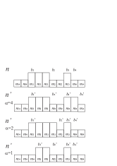
Figure S1: Upper-most figure schematically shows an example Eq. (S10) of $\{b_{\alpha},m_{\alpha}\}_{\alpha=1}^{2N}$ for $N=2$ and $L=10$. Other figures show examples of $\bm{n}^{\prime}$ satisfying Eq. (S11).

The states $|\bm{n}\rangle\in V_{N}$ with $N\in[1,L/2-1]$ contain at least a pair of adjacent sites with spin contents $``11"$ or $``00"$ (otherwise $\bm{n}$ would belong to $V_{0}$ or $V_{L/2}$) and thus also a segment of consecutive three sites with spin contents $``011"$ or $``100"$. In our notation, ${}^{\exists}\alpha\in[1,2N],\quad b_{\alpha+1}-b_{\alpha}\geq 2$.

The next lemma implies that an action of $\hat{\mathcal{H}}_{\rm p0}$ on $|\bm{n}\rangle$ can shift one of the boundaries $b_{\alpha}(\bm{n})$ by one site to the right when $b_{\alpha+1}(\bm{n})-b_{\alpha}(\bm{n})\geq 2$.

Lemma S2
When $b_{\alpha+1}-b_{\alpha}\geq 2$ for ${}^{\exists}\alpha\in[1,2N]$ in $\bm{n}\in V_{N}$ with $N\in[1,L/2-1]$, $\bm{n}\sim\bm{n}^{\prime}$, where

$$b_{\beta}(\bm{n}^{\prime}) =b_{\beta}(\bm{n})+\delta_{\beta,\alpha}$$ (S11a)

$$m_{\beta}(\bm{n}^{\prime}) =m_{\beta}(\bm{n})$$ (S11b)

for $\beta\in[1,2N]$. Figure S1 shows examples of $\bm{n}$ and $\bm{n}^{\prime}$ satisfying Eq. (S11).

Proof.

The spin configuration $\bm{n}$ in the three consecutive sites $i=b_{\alpha}-1,b_{\alpha},b_{\alpha}+1$ is

$$\bm{n}=(\cdots,m_{\alpha-1},m_{\alpha},m_{\alpha},\cdots).$$ (S12)

It follows from Eq. (19) that

$$M(\bm{n}^{\prime},\bm{n};1)=\frac{D}{2}(-1)^{\delta(\bm{n})+\delta(\bm{n}^{\prime})}\langle\bm{n}^{\prime}|\hat{h}_{b_{\alpha}}|\bm{n}\rangle>0.$$ (S13)

∎

Lemma S3
For $|\bm{n}\rangle\in V_{N}$ with $N\in[1,L/2-1]$,

$$T(\bm{n})\sim\bm{n}.$$ (S14)

Proof.

The relation between $\bm{n}$ and $T(\bm{n})$ is expressed as

$$b_{\beta}(T(\bm{n})) =b_{\beta}(\bm{n})+1$$ (S15a)

$$m_{\beta}(T(\bm{n})) =m_{\beta}(\bm{n})$$ (S15b)

for $\beta\in[1,2N]$.

For $\bm{n}\in V_{N}$ with $N\in[1,L/2-1]$, ${}^{\exists}\alpha\in[1,2N],\quad b_{\alpha+1}-b_{\alpha}\geq 2$.

For $\bm{n}^{\prime}$ defined by Eq. (S11), we note that $b_{\alpha}(\bm{n}^{\prime})-b_{\alpha-1}(\bm{n}^{\prime})=b_{\alpha}(\bm{n})-b_{\alpha-1}(\bm{n})+1\geq 2$ and thus find that we can shift $b_{\alpha-1}(\bm{n}^{\prime})$ by one site to the right by an action of $\hat{\mathcal{H}}_{\rm p0}$ on $|\bm{n}^{\prime}\rangle$,

$$M(\bm{n}^{\prime\prime},\bm{n}^{\prime};1)=\frac{D}{2}>0,$$ (S16)

i.e., $\bm{n}^{\prime}\sim\bm{n}^{\prime\prime}$ for $\bm{n}^{\prime}$ and $\bm{n}^{\prime\prime}$ defined by

$$b_{\beta}(\bm{n}^{\prime\prime}) =b_{\beta}(\bm{n}^{\prime})+\delta_{\beta,\alpha-1}$$ (S17a)

$$m_{\beta}(\bm{n}^{\prime\prime}) =m_{\beta}(\bm{n}^{\prime})$$ (S17b)

for $\beta\in[1,2N]$. Note that $b_{\alpha-1}(\bm{n}^{\prime\prime})-b_{\alpha-2}(\bm{n}^{\prime\prime})=b_{\alpha-1}(\bm{n}^{\prime})-b_{\alpha-2}(\bm{n}^{\prime})+1\geq 2$ and thus we can shift $b_{\alpha-2}(\bm{n}^{\prime\prime})$ by one site to the right in a way similar to the above procedure. By repeating these procedures as schematically shown in Fig. S2, we can shift all $b_{\beta}(\bm{n})$ for $\beta\in[1,2N]$ by one site to the right and arrive at

$$\bm{n}\sim\bm{n}^{\prime}\sim\bm{n}^{\prime\prime}\sim\cdots\sim T(\bm{n}),$$ (S18)

i.e., Eq. (S14).

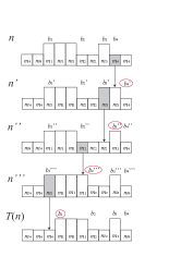
Figure S2: Schematics illustrating relation $\bm{n}\sim T(\bm{n})$ (Lemma S3). The arrows represent the action of the local Hamiltonian $\hat{h}_{i}$, which changes $n_{i}$ represented by shaded squares by one. The characters for updated $b_{\alpha}$s by this action are encircled.

∎

Proof of Lemma 2

Proof.

For arbitrary $\bm{n}$ and $\bm{n}^{\prime}\in V_{N}$ with $N\in[1,L/2-1]$, there exists an integer $l$ such that

$$b_{2N}(T^{l}(\bm{n}^{\prime})) =b_{2N}(\bm{n})$$ (S19a)

$$m_{\beta}(T^{l}(\bm{n}^{\prime})) =m_{\beta}(\bm{n})$$ (S19b)

for $\beta\in[1,2N]$. It thus suffices to show that $\bm{n}\sim\bm{n}^{\prime}$ for $\bm{n},\bm{n}^{\prime}\in V_{N}$ with $N\in[1,L/2-1]$ satisfying

$$b_{2N}(\bm{n}^{\prime}) =b_{2N}(\bm{n})$$ (S20a)

$$m_{\beta}(\bm{n}^{\prime}) =m_{\beta}(\bm{n})$$ (S20b)

for $\beta\in[1,2N]$. For $\bm{n}$ and $\bm{n}^{\prime}$ satisfying Eq. (S20), we define $\{\bm{n}^{(\alpha)},\bm{n}^{{}^{\prime}(\alpha)}\}_{\alpha=1}^{2N}\in V_{N}$ with $N\in[1,L/2-1]$ by

$$b_{\beta}(\bm{n}^{(\alpha)}) =\left\{\begin{array}[]{cl}\mbox{Max}(b_{\beta}(\bm{n}^{\prime}),b_{\beta}(\bm{n})),&\beta\in[\alpha,2N]\\ b_{\beta}(\bm{n}),&\mbox{otherwise}\end{array}\right.$$ (S21c)

$$m_{\beta}(\bm{n}^{(\alpha)}) =m_{\beta}(\bm{n}),\quad\beta\in[1,2N]$$ (S21d)

and

$$b_{\beta}(\bm{n}^{{}^{\prime}(\alpha)}) =\left\{\begin{array}[]{cl}\mbox{Max}(b_{\beta}(\bm{n}^{\prime}),b_{\beta}(\bm{n}))&\beta\in[\alpha,2N]\\ b_{\beta}(\bm{n}^{\prime})&\mbox{otherwise}\end{array}\right.$$ (S22c)

$$m_{\beta}(\bm{n}^{{}^{\prime}(\alpha)}) =m_{\beta}(\bm{n}^{\prime}),\quad\beta\in[1,2N].$$ (S22d)

By definition,

$$\bm{n}^{(2N)} =\bm{n}$$ (S23a)

$$\bm{n}^{{}^{\prime}(2N)} =\bm{n}^{\prime}$$ (S23b)

$$\bm{n}^{(1)} =\bm{n}^{{}^{\prime}(1)}.$$ (S23c)

Examples of $\{\bm{n}^{(\alpha)},\bm{n}^{{}^{\prime}(\alpha)}\}_{\alpha=1}^{2N}\in V_{N}$ for $N=2$ are shown in Fig. S3.

We show that $\bm{n}^{(\alpha)}\sim\bm{n}^{(\alpha-1)}$ for $\alpha\in[2,2N]$. When $b_{\alpha-1}(\bm{n})\geq b_{\alpha-1}(\bm{n}^{\prime})$, $\bm{n}^{(\alpha)}=\bm{n}^{(\alpha-1)}$ and thus we focus on the case where $b_{\alpha-1}(\bm{n})<b_{\alpha-1}(\bm{n}^{\prime})$. We introduce $\bm{n}^{(\alpha,a)}$ for $a\in[0,b_{\alpha-1}(\bm{n}^{\prime})-b_{\alpha-1}(\bm{n})]$ by

$$b_{\beta}(\bm{n}^{(\alpha,a)}) =\left\{\begin{array}[]{cl}b_{\alpha-1}(\bm{n}^{(\alpha)})+a,&\beta=\alpha-1\\ b_{\beta}(\bm{n}^{(\alpha)}),&\mbox{otherwise}\end{array}\right.$$ (S24c)

$$m_{\beta}(\bm{n}^{(\alpha,a)}) =m_{\beta}(\bm{n}),\quad\beta\in[1,2N].$$ (S24d)

Note that

$$\bm{n}^{(\alpha,0)}=\bm{n}^{(\alpha)},\quad\bm{n}^{(\alpha,b_{\alpha-1}(\bm{n}^{\prime})-b_{\alpha-1}(\bm{n}))}=\bm{n}^{(\alpha-1)}$$ (S25)

Examples of $\bm{n}^{(\alpha,a)}$ are shown in Fig. S4.

When $a\in[0,b_{\alpha-1}(\bm{n}^{\prime})-b_{\alpha-1}(\bm{n})-1]$, it holds that

$$b_{\alpha}(\bm{n}^{(\alpha,a)})-b_{\alpha-1}(\bm{n}^{(\alpha,a)})$$

$$= b_{\alpha}(\bm{n}^{(\alpha)})-b_{\alpha-1}(\bm{n}^{(\alpha)})-a$$

$$= b_{\alpha}(\bm{n}^{(\alpha)})-b_{\alpha-1}(\bm{n}^{\prime})-a$$

$$\geq b_{\alpha}(\bm{n}^{(\alpha)})-b_{\alpha-1}(\bm{n})+1$$

$$= \underbrace{b_{\alpha}(\bm{n}^{(\alpha)})-b_{\alpha-1}(\bm{n}^{(\alpha)})}_{\geq 1}+1\geq 2.$$ (S26)

From Lemma S2, it follows that $\bm{n}^{(\alpha,a)}\sim\bm{n}^{(\alpha,a+1)}$ for $a\in[0,b_{\alpha-1}(\bm{n}^{\prime})-b_{\alpha-1}(\bm{n})]$ and thus $\bm{n}^{(\alpha)}\sim\bm{n}^{(\alpha-1)}$ (See Eq. (S25)) for $\alpha\in[2,2N]$. From the relation and Eq. (S23), $\bm{n}\sim\bm{n}^{(1)}$. Similarly, $\bm{n}^{\prime}\sim\bm{n}^{{}^{\prime}(1)}=\bm{n}^{(1)}$ holds and it follows that $\bm{n}\sim\bm{n}^{\prime}$. ∎

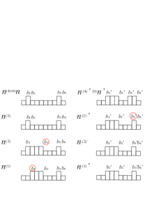
Figure S3: Examples of $\{\bm{n}^{(\alpha)},\bm{n}^{{}^{\prime}(\alpha)}\}_{\alpha=1}^{2N}$, which are defined, respectively, by Eqs. (S21) and (S22). The characters for updated $b_{\alpha}$s are encircled.

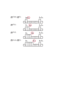
Figure S4: Examples of $\bm{n}^{(\alpha,a)}$ defined by Eq. (S24). The characters for updated $b_{\alpha}$s are encircled.

S2 Derivation of Eq. (40)

$$\hat{T}^{\dagger}\hat{U}\hat{T} =\hat{U}|_{\hat{P}_{j}^{(S-f)}\rightarrow\hat{P}_{j-1}^{(S-f)}}$$

$$=\exp\left[{\rm i}\pi\sum_{j=1}^{L}\sum_{f=1}^{2S}\sum_{a=0}^{2S-f}jf\hat{P}_{j-1}^{(S-a)}\hat{P}_{j}^{(S-a-f)}\right]$$

$$=\uwave{\exp\left[{\rm i}\pi\sum_{j=0}^{L-1}\sum_{f=1}^{2S}\sum_{a=0}^{2S-f}jf\hat{P}_{j}^{(S-a)}\hat{P}_{j+1}^{(S-a-f)}\right]}$$

$$\times\exp\left[{\rm i}\pi\dashuline{\sum_{j=0}^{L-1}\sum_{f=1}^{2S}\sum_{a=0}^{2S-f}f\hat{P}_{j}^{(S-a)}\hat{P}_{j+1}^{(S-a-f)}}\right]$$

In the third equality, we replaced the dummy index $j$ by $j+1$. We will show that (i) the Expression underlined by a wavy line is equal to $\hat{U}$ and (ii) that underlined by a dashed line coincides with

$$\dashuline{\sum_{j=0}^{L-1}\sum_{f=1}^{2S}\sum_{a=0}^{2S-f}f\hat{P}_{j}^{(S-a)}\hat{P}_{j+1}^{(S-a-f)}}=\sum_{f}f\hat{N}_{f}.$$ (S28)

Concerning (i), we find that

$$\uwave{\exp\left[{\rm i}\pi\sum_{j=0}^{L-1}\sum_{f=1}^{2S}\sum_{a=0}^{2S-f}jf\hat{P}_{j}^{(S-a)}\hat{P}_{j+1}^{(S-a-f)}\right]}$$

$$=\hat{U}\exp\left[-{\rm i}\pi L\sum_{f=1}^{2S}\sum_{a=0}^{2S-f}f\hat{P}_{L}^{(S-a)}\hat{P}_{L+1}^{(S-a-f)}\right]$$

$$=\hat{U}.$$ (S29)

In the last equality, we have used that $L$ is even.

Concerning (ii), we find that the left hand side of Eq. (S28) is rewritten as

$$\sum_{j=0}^{L-1}\sum_{1\leq a\leq a+f\leq 2S}f\hat{P}_{j}^{(S-a)}\hat{P}_{j+1}^{(S-a-f)}$$

$$= \sum_{j=0}^{L-1}\sum_{1\leq a\leq b\leq 2S}(b-a)\hat{P}_{j}^{(S-a)}\hat{P}_{j+1}^{(S-b)}$$ (S30)

With use of Eqs. (28) and (29), the right hand side of Eq. (S28) is rewritten as

$$\sum_{f=1}^{2S-1}f\sum_{i=1}^{L}\left(\sum_{a<f}\hat{P}_{i-1}^{(S-a)}-\sum_{b>f}\hat{P}_{i+1}^{(S-b)}\right)\hat{P}_{i}^{(S-f)}$$

$$+2S\sum_{i=1}^{L}\sum_{a<f}\hat{P}_{i-1}^{(S-a)}\hat{P}_{i}^{(S-f)}$$

$$=\sum_{i=1}^{L}\left[\sum_{1\leq a<f\leq 2S}f\hat{P}_{i}^{(S-a)}\hat{P}_{i+1}^{(S-f)}-\sum_{1\leq f\leq b\leq 2S}f\hat{P}_{i}^{(S-f)}\hat{P}_{i+1}^{(S-b)}\right]$$

$$=\sum_{i=1}^{L}\left(\sum_{1\leq a<b\leq 2S}(b-a)\hat{P}_{i}^{(S-a)}\hat{P}_{i+1}^{(S-b)}\right),$$ (S31)

which concides with Eq.(S30) and thus the relation Eq. (S28) follows.

S3 Derivation of Eq. (51)

We will derive from Eq. (50) to Eq. (51). In Eq. (50), the operator $\hat{\mathcal{S}}_{i}^{x}(a,b)\hat{P}_{i-1}^{(S-a)}\hat{P}_{i+1}^{(S-b)}$ does not contain $\hat{P}_{j}^{(S-f)}$ with $j\neq,i,i\pm 1$ and thus the part containing these projection operators in $\hat{U}$ and $\hat{U}^{\dagger}$ can be dropped. Further $\hat{P}_{i\pm 1}^{(S-f)}$ in $\hat{U}$ and $\hat{U}^{\dagger}$ can be replaced as

$$\hat{P}_{i-1}^{(S-f)}\rightarrow\hat{1}\delta_{f,a}\quad\hat{P}_{i+1}^{(S-f)}\rightarrow\hat{1}\delta_{f,b}$$ (S32)

owing to the presence of $\hat{P}_{i-1}^{(S-a)}\hat{P}_{i+1}^{(S-b)}$ in Eq. (50). With use of it, the summand in Eq. (50) reduces to

$$\hat{U}\hat{\mathcal{S}}_{i}^{x}(a,b)\hat{P}_{i-1}^{(S-a)}\hat{P}_{i+1}^{(S-b)}\hat{U}^{\dagger}$$

$$= \hat{u}_{i}\hat{\mathcal{S}}_{i}^{x}(a,b)\hat{u}_{i}^{\dagger}\hat{P}_{i-1}^{(S-a)}\hat{P}_{i+1}^{(S-b)}$$ (S33)

with

$$\hat{u}_{i}=\exp\left[{\rm i}\pi\sum_{c=a}^{b}((c-a)(i-1)+(b-c)i)\hat{P}_{i}^{(S-c)}\right].$$ (S34)

When $a\geq b$, $\hat{u}_{i}=\hat{1}$ and thus

$$\hat{u}_{i}\hat{\mathcal{S}}_{i}^{x}(a,b)\hat{u}_{i}^{\dagger}=\hat{\mathcal{S}}_{i}^{x}(a,b)$$ (S35)

for $a\geq b$. We thus consider the case when $a<b$. The operator

$$\hat{u}_{i}\hat{\mathcal{S}}_{i}^{x}(a,b)\hat{u}_{i}^{\dagger}$$ (S36)

is a single site operator for the $i$-th site. From the operator contents in $\hat{\mathcal{S}}_{i}^{x}(a,b)$, it follows that

$$\langle n_{i}|\hat{u}_{i}\hat{\mathcal{S}}_{i}^{x}(a,b)\hat{u}_{i}^{\dagger}|n^{\prime}_{i}\rangle=0$$ (S37)

unless $n_{i}=n^{\prime}_{i}\pm 1$. With use of this property, Eq. (S36) is rewritten as

$$\hat{u}_{i}\hat{\mathcal{S}}_{i}^{x}(a,b)\hat{u}_{i}^{\dagger}$$

$$=\sum_{0\leq k,k+1\leq 2S}\hat{P}_{i}^{(S-k)}\hat{u}_{i}\hat{\mathcal{S}}_{i}^{x}(a,b)\hat{u}_{i}^{\dagger}\hat{P}_{i}^{(S-k-1)}$$ (S38)

$$+\sum_{0\leq k,k-1\leq 2S}\hat{P}_{i}^{(S-k)}\hat{u}_{i}\hat{\mathcal{S}}_{i}^{x}(a,b)\hat{u}_{i}^{\dagger}\hat{P}_{i}^{(S-k+1)}.$$ (S39)

In Eq. (S38), the operator $\hat{P}_{i}^{(S-c)}$ in $\hat{u}_{i}$ can be replaced by $\hat{1}\delta_{k,c}$ owing to the presence of $\hat{P}_{i}^{(S-k)}$. With use of it, $\hat{u}_{i}$ in Eq. (S38) can be reduced to

$$\hat{u}_{i}\rightarrow(-1)^{bi-a(i-1)-k}\hat{1}.$$ (S40)

Similarly, $\hat{P}_{i}^{(S-c)}$ in $\hat{u}_{i}^{\dagger}$ can be replaced by $\hat{1}\delta_{k+1,c}$ and $\hat{u}_{i}^{\dagger}$ in Eq. (S38) reduces to

$$\hat{u}_{i}^{\dagger}\rightarrow(-1)^{-bi+a(i-1)+k+1}\hat{1}.$$ (S41)

From (S40) and (S41), Eq. (S38) reduces to

$$-\sum_{0\leq k,k+1\leq 2S}\hat{P}_{i}^{(S-k)}\hat{\mathcal{S}}_{i}^{x}(a,b)\hat{P}_{i}^{(S-k-1)}$$ (S42)

Similarly, Eq. (S39) becomes

$$-\sum_{0\leq k,k-1\leq 2S}\hat{P}_{i}^{(S-k)}\hat{\mathcal{S}}_{i}^{x}(a,b)\hat{P}_{i}^{(S-k+1)}.$$ (S43)

From (S42) and (S43),

$$\hat{u}_{i}\hat{\mathcal{S}}_{i}^{x}(a,b)\hat{u}_{i}^{\dagger}$$

$$= -\sum_{0\leq k,k+1\leq 2S}\hat{P}_{i}^{(S-k)}\hat{\mathcal{S}}_{i}^{x}(a,b)\hat{P}_{i}^{(S-k-1)}$$

$$-\sum_{0\leq k,k-1\leq 2S}\hat{P}_{i}^{(S-k)}\hat{\mathcal{S}}_{i}^{x}(a,b)\hat{P}_{i}^{(S-k+1)}$$

$$=-\hat{\mathcal{S}}_{i}^{x}(a,b).$$ (S44)

for $a<b$. From Eqs. (50), (S33), (S44), and (S35), Eq. (51) follows.

S4 Proof of Lemma 6

As a statement equivalent to Eq. (39), we prove

$$\langle T(\bm{n})|(-\hat{\mathcal{H}}^{\prime}_{\rm p0})^{l}|\bm{n}\rangle\neq 0$$ (S45)

because the off-diagonal matrix elements of $\hat{\mathcal{H}}_{{\rm p}}$ coincide with those of $\hat{\mathcal{H}}^{\prime}_{{\rm p}}$ up to an overall sign and the latter stems from those of $\hat{\mathcal{H}}^{\prime}_{\rm p0}$. Further, all the off-diagonal matrix elements of $-\hat{\mathcal{H}}^{\prime}_{\rm p0}$ are non-negative and thus it suffices to find a set of the intermediate states $\{\bm{n}^{(1)},\bm{n}^{(2)},\cdots,\bm{n}^{(l-1)}\}$ satisfying

$$\langle\bm{n}^{(a)}|\hat{\mathcal{H}}^{\prime}_{\rm p0}|\bm{n}^{(a-1)}\rangle\neq 0,\quad\mbox{for }a=[1,l],$$ (S46)

where $\bm{n}^{(0)}$ and $\bm{n}^{(l)}$, respectively, read as $\bm{n}$ and $T(\bm{n})$.

We find, from Eqs. (51) and (47), the support of the local Hamiltonian $\hat{h}^{\prime}_{i}$. $\hat{h}^{\prime}_{i}|\bm{n}\rangle$ can be nonzero only when the following two conditions are satisfied:

$$n_{i-1}\neq n_{i+1}$$ (S47a)

$${\rm min}(n_{i-1},n_{i+1})\leq n_{i}\leq{\rm max}(n_{i-1},n_{i+1}).$$ (S47b)

Let $\mathcal{V}(i)$ be the set of $\bm{n}$ satisfying Eqs. (S47a) and (S47b). The condition Eq. (S47a) comes from the factor $|a-b|\hat{P}_{i-1}^{(S-a)}\hat{P}_{i+1}^{(S-b)}$ in Eq. (51) and the other condition Eq. (S47b) does from the factor $\hat{P}_{i-1}^{(S-a)}\hat{P}_{i+1}^{(S-b)}\left(\sum_{k={\rm min}(a,b)}^{{\rm max}(a,b)}\hat{P}_{i}^{(S-a)}\right)$ in Eq. (51) with Eq. (47).

The local Hamiltonian $\hat{h}^{\prime}_{i}$ commutes with $\hat{S}_{j}^{z}$ for $j\neq i$ and thus $\langle\bm{n}^{\prime}|\hat{h}^{\prime}_{i}|\bm{n}\rangle$ reduces to

$$\langle\bm{n}^{\prime}|\hat{h}^{\prime}_{i}|\bm{n}\rangle$$

$$=|n_{i-1}-n_{i+1}|\langle n_{i}^{\prime}|\hat{S}_{i}^{x}|n_{i}\rangle_{i}\prod_{j(\neq i)}\delta_{n^{\prime}_{j},n_{j}}, \mbox{for }\bm{n}^{\prime},\bm{n}\in\mathcal{V}(i),$$ (S48)

which can be summarized as

$$\langle\bm{n}^{\prime}|\hat{h}^{\prime}_{i}|\bm{n}\rangle$$

$$\left\{\begin{array}[]{cc}>0,&\bm{n}^{\prime},\bm{n}\in\mathcal{V}(i)\mbox{ and }n^{\prime}_{j}=n_{j}\pm\delta_{i,j},\mbox{ for }j\in[1,L]\\ =0,&\mbox{otherwise.}\end{array}\right.$$ (S51)

From Eq. (S51), it follows that

$$\langle\bm{n}^{\prime}|\hat{h}^{\prime}_{k}|\bm{n}\rangle=0,\mbox{ for }k\neq i$$ (S52)

$$\langle\bm{n}^{\prime}|\hat{\mathcal{H}}^{\prime}_{\rm p0}|\bm{n}\rangle=-D\langle\bm{n}^{\prime}|\hat{h}^{\prime}_{i}|\bm{n}\rangle<0,$$

$$\mbox{when }\bm{n}^{\prime},\bm{n}\in\mathcal{V}(i)\mbox{ and }n^{\prime}_{j}=n_{j}\pm\delta_{i,j},\mbox{ for }j\in[1,L].$$ (S53)

Below we provide a proof of Lemma 6 using Eq. (S48). It is convenient for this purpose to parametrize $\bm{n}$ in the following way. For a given $\bm{n}$, let $B=B(\bm{n})$ be the set of $i$ such that $n_{i-1}\neq n_{i}$ and $d_{B}$ be the number of elements of $B$. We label these elements in $B(\bm{n})=\{b_{\alpha}\}$ in increasing order

$$1\leq b_{1}<b_{2}\cdots<b_{d_{B}}\leq L.$$ (S54)

We define $m_{\alpha}\in[0,2S]$ for $\alpha=[1,d_{B}]$ by

$$m_{\alpha}=n_{i},\mbox{ with }i=b_{\alpha}.$$ (S55)

We also define $b_{d_{B}+1}$ and $m_{d_{B}+1}$, respectively as, $b_{1}+L$ and $m_{1}$. By definition, $m_{\alpha}\neq m_{\alpha+1}$ for $\alpha=[1,d_{B}]$. When $L=8$ and $\bm{n}=00133000$, for example (see Fig. S5), $d_{B}=3$ and

$$b_{1}=3,\quad b_{2}=4,\quad b_{3}=6,\quad b_{4}=11$$ (S56a)

$$m_{1}=1,\quad m_{2}=3,\quad m_{3}=0,\quad m_{4}=1.$$ (S56b)

Figure S5: Upper panel: Example Eq. (S56) of $\{b_{\alpha},m_{\alpha}\}_{\alpha=1}^{d_{B}}$ for $\bm{n}=00133000$. $d_{B}=3$ and $L=8$. Lower panel: Example of $\bm{n}^{\prime}$ defined by Eq. (S59).

In these notations, the relation between $\bm{n}$ and $T(\bm{n})$ reads

$$b_{\beta}(T(\bm{n})) =b_{\beta}(\bm{n})+1$$ (S57a)

$$m_{\beta}(T(\bm{n})) =m_{\beta}(\bm{n})$$ (S57b)

for $\beta\in[1,d_{B}]$.

To prove Lemma 6, we consider the following two cases separately:

• Case 1. ${}^{\exists}\alpha\in[1,d_{B}],\quad b_{\alpha+1}-b_{\alpha}\geq 2$.

• Case 2. ${}^{\forall}\alpha\in[1,d_{B}],\quad b_{\alpha+1}-b_{\alpha}=1$ (mod $L$).

Case 1
For case 1, we consider the situation where ${}^{\exists}\alpha\in[1,d_{B}-1],\quad b_{\alpha+1}-b_{\alpha}\geq 2$. For this case, the portion of the spin configuration $\bm{n}$ concerning the three consecutive sites $i=b_{\alpha}-1,b_{\alpha},b_{\alpha}+1$ is

$$\bm{n}=(\cdots,m_{\alpha-1},m_{\alpha},m_{\alpha},\cdots)$$ (S58)

from which we see that $\bm{n}\in\mathcal{V}(b_{\alpha})$ because Eq. (S58) satisfies Eqs. (S47a) and (S47b) with $i=b_{\alpha}$. We assume that $m_{\alpha-1}-m_{\alpha}>0$. The case where $m_{\alpha-1}<m_{\alpha}$ can be dealt with in a way similar to the following argument. We show that the matrix element $\langle\bm{n}^{\prime}|(-\hat{\mathcal{H}}_{\rm p0})^{(m_{\alpha-1}-m_{\alpha})}|\bm{n}\rangle>0$, where

$$n^{\prime}_{j}=n_{j}+(m_{\alpha-1}-m_{\alpha})\delta_{i,j}.$$ (S59)

In a way similar to Eq. (S58)$,\bm{n}^{\prime}$ is expressed as

$$\bm{n}^{\prime}=(\cdots,m_{\alpha-1},m_{\alpha-1},m_{\alpha},\cdots)$$ (S60)

and

$$b_{\beta}(\bm{n}^{\prime}) =b_{\beta}(\bm{n})+\delta_{\beta,\alpha}$$ (S61a)

$$m_{\beta}(\bm{n}^{\prime}) =m_{\beta}(\bm{n})$$ (S61b)

for $\beta\in[1,d_{B}]$. Example of $\bm{n}^{\prime}$ is shown in the lower panel in

We introduce a series of states $\{\bm{n}^{(0)},\bm{n}^{(1)},\bm{n}^{(2)},\cdots,\bm{n}^{(m_{\alpha-1}-m_{\alpha})}\}$ as

$$n^{(a)}_{j}=n_{j}+a\delta_{i,j},\quad\mbox{for }j\in[1,L],$$ (S62)

i.e.

$$\bm{n}^{(a)}=(\cdots,m_{\alpha-1},m_{\alpha}+a,m_{\alpha},\cdots)$$ (S63)

for $a=[0,m_{\alpha-1}-m_{\alpha}]$. Note that $\bm{n}^{(0)}=\bm{n}$ and $\bm{n}^{(m_{\alpha-1}-m_{\alpha})}=\bm{n}^{\prime}$. We see that $\bm{n}^{(a)}\in\mathcal{V}(b_{\alpha})$ for $a\in[0,m_{\alpha-1}-m_{\alpha}]$ and

$$n^{(a)}_{j}=n^{(a-1)}_{j}+\delta_{i,j},\quad\mbox{for }j\in[1,L].$$ (S64)

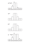
Figure S6: Examples of $n^{(a)}$ defined by Eq. (S62) or (S63) where $\bm{n}=00133000$, $\bm{n}^{\prime}=00133300$, $i=6$, and $L=8$.

From this observation and Eq. (S53), we find that

$$\langle\bm{n}^{(a)}|\hat{\mathcal{H}}^{\prime}_{\rm p0}|\bm{n}^{(a-1)}\rangle<0,\quad\mbox{for }a\in[1,m_{\alpha-1}-m_{\alpha}],$$ (S65)

from which

$$\langle\bm{n}^{\prime}|(-\hat{\mathcal{H}}^{\prime}_{\rm p0})^{m_{\alpha-1}-m_{\alpha}}|\bm{n}\rangle>0$$ (S66)

follows for $\bm{n}$ (Eq. (S58)) and $\bm{n}^{\prime}$ (Eq. (S60)) . From Eqs. (S61) and (S66), we see that multiple actions of $\hat{\mathcal{H}}^{\prime}_{\rm p0}$ on $|\bm{n}\rangle$ can shift one of the boundaries $b_{\alpha}(\bm{n})$ by one site to the right when $b_{\alpha+1}(\bm{n})-b_{\alpha}(\bm{n})\geq 2$. We note that $b_{\alpha}(\bm{n}^{\prime})-b_{\alpha-1}(\bm{n}^{\prime})=b_{\alpha}(\bm{n})-b_{\alpha-1}(\bm{n})+1\geq 2$ and thus find that we can shift $b_{\alpha-1}(\bm{n}^{\prime})$ by one site to the right by multiple actions of $\hat{\mathcal{H}}^{\prime}_{\rm p0}$ on $|\bm{n}^{\prime}\rangle$, viz,

$$\langle\bm{n}^{\prime\prime}|(-\hat{\mathcal{H}}^{\prime}_{\rm p0})^{m_{\alpha-2}-m_{\alpha-1}}|\bm{n}^{\prime}\rangle>0$$ (S67)

for $\bm{n}^{\prime}$ (Eq. (S60)) and $\bm{n}^{\prime\prime}$ satisfying

$$b_{\beta}(\bm{n}^{\prime\prime}) =b_{\beta}(\bm{n}^{\prime})+\delta_{\beta,\alpha-1}$$ (S68a)

$$m_{\beta}(\bm{n}^{\prime\prime}) =m_{\beta}(\bm{n}^{\prime})$$ (S68b)

for $\beta\in[1,d_{B}]$. Note that $b_{\alpha-1}(\bm{n}^{\prime\prime})-b_{\alpha-2}(\bm{n}^{\prime\prime})=b_{\alpha-1}(\bm{n}^{\prime})-b_{\alpha-2}(\bm{n}^{\prime})+1\geq 2$ and thus we can shift $b_{\alpha-2}(\bm{n}^{\prime\prime})$ by one site to the right in a way similar to the above procedure. By repeating these procedures, we can shift all $b_{\beta}(\bm{n})$ for $\beta\in[1,d_{B}]$ by one site to the right and arrive at $T(\bm{n})$ satisfying Eq. (S57).
 
Case 2
We discuss Case 2, where $\beta\in[1,d_{B}],\quad b_{\beta+1}-b_{\beta}\equiv 1$ (mod $L$). In Lemma 6, we consider $\bm{n}\in V_{\mu}(\{N_{f}\})$ with $d(V_{\mu}(\{N_{f}\}))>1$ and thus there exists $\alpha\in[1,d_{B}]$ such that $\bm{n}\in\mathcal{V}(b_{\alpha})$. In this case, the spin configuration in $\bm{n}$ for consecutive three sites $i=b_{\alpha}-1,b_{\alpha},b_{\alpha}+1$ is given by

$$\bm{n}=(\cdots,m_{\alpha-1},m_{\alpha},m_{\alpha+1},\cdots).$$ (S69)

We assume that $m_{\alpha-1}>m_{\alpha}>m_{\alpha+1}$. The case where $m_{\alpha-1}<m_{\alpha}<m_{\alpha+1}$ can be discussed in a similar way.

We introduce a series of the states $\{\bm{n}^{(1)},\bm{n}^{(2)},\cdots,\bm{n}^{(m_{\alpha-1}-m_{\alpha})}\}$ satisfying Eq. (S62). In the present case, Eq. (S63) should be replaced by

$$\bm{n}^{(a)}=(\cdots,m_{\alpha-1},m_{\alpha}+a,m_{\alpha+1},\cdots)$$ (S70)

for $a=[1,m_{\alpha-1}-m_{\alpha}]$. We can show that

$$\langle\bm{n}^{\prime}|(-\hat{\mathcal{H}}^{\prime}_{\rm p0})^{m_{\alpha-1}-m_{\alpha}}|\bm{n}\rangle>0$$ (S71)

for $\bm{n}^{\prime}=\bm{n}^{(m_{\alpha-1}-m_{\alpha})}$ in a way similar to the proof of Eq. (S66). Spin configuration in $\bm{n}^{\prime}$ for consecutive three sites $i=b_{\alpha}-1,b_{\alpha},b_{\alpha}+1$ is given by

$$\bm{n}^{\prime}=(\cdots,m_{\alpha-1},m_{\alpha-1},m_{\alpha+1},\cdots).$$ (S72)

and thus the argument for Case 1 is applicable to $\bm{n}^{\prime}$, i.e., there exists a positive integer $l$ such that

$$\langle T(\bm{n}^{\prime})|(-\hat{\mathcal{H}}^{\prime}_{\rm p0})^{l}|\bm{n}^{\prime}\rangle>0.$$ (S73)

Further

$$\langle T(\bm{n})|(-\hat{\mathcal{H}}^{\prime}_{\rm p0})^{m_{\alpha-1}-m_{\alpha}}|T(\bm{n}^{\prime})\rangle$$

$$=\langle\bm{n}|(-\hat{\mathcal{H}}^{\prime}_{\rm p0})^{{m_{\alpha-1}-m_{\alpha}}}|\bm{n}^{\prime}\rangle>0$$ (S74)

follows from translational invariance of $\hat{\mathcal{H}}^{\prime}_{\rm p0}$ and Eq. (S71). Combining Eqs. (S71), (S73), and (S74), we arrive at Lemma 6 for Case 2. Figure S7 schematically shows that Eqs. (S71) (left column), (S73) (right column), and (S74) (two figures in the bottom).

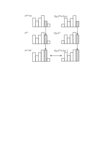
Figure S7: Examples of Eqs. (S71) (left column), Eq. (S73) (right column), and Eq. (S74) (two figures in the bottom) for Case 2.

References

- Dzyaloshinsky [1958] I. Dzyaloshinsky, A thermodynamic theory of “weak” ferromagnetism of antiferromagnetics, Journal of Physics and Chemistry of Solids 4, 241 (1958).
- Moriya [1960] T. Moriya, Anisotropic Superexchange Interaction and Weak Ferromagnetism, Physical Review 120, 91 (1960).
- Bogdanov and Yablonskii [1989] A. N. Bogdanov and D. A. Yablonskii, Thermodynamically stable “vortices” in magnetically ordered crystals. The mixed state of magnets, Sov. Phys. JETP 68, 101 (1989).
- Bogdanov and Hubert [1994] A. Bogdanov and A. Hubert, Thermodynamically stable magnetic vortex states in magnetic crystals, Journal of Magnetism and Magnetic Materials 138, 255 (1994).
- Pappas et al. [2009] C. Pappas, E. Lelièvre-Berna, P. Falus, P. M. Bentley, E. Moskvin, S. Grigoriev, P. Fouquet, and B. Farago, Chiral Paramagnetic Skyrmion-like Phase in MnSi, Phys. Rev. Lett. 102, 197202 (2009).
- Mühlbauer et al. [2009] S. Mühlbauer, B. Binz, F. Jonietz, C. Pfleiderer, A. Rosch, A. Neubauer, R. Georgii, and P. Böni, Skyrmion lattice in a chiral magnet, Science 323, 915 (2009).
- Yu et al. [2010] X. Z. Yu, Y. Onose, N. Kanazawa, J. H. Park, J. H. Han, Y. Matsui, N. Nagaosa, and Y. Tokura, Real-Space Observation of a Two-Dimensional Skyrmion Crystal, Nature 465, 901 (2010).
- Nagaosa and Tokura [2013] N. Nagaosa and Y. Tokura, Topological properties and dynamics of magnetic skyrmions, Nature nanotechnology 8, 899 (2013).
- Dzyaloshinskii [1965] I. Dzyaloshinskii, Theory of Helicoidal Structures in Antiferromagnets. III , Sov. Phys. JETP 20, 665 (1965).
- Moriya and Miyadai [1982] T. Moriya and T. Miyadai, Evidence for the helical spin structure due to antisymmetric exchange interaction in Cr1/3NbS2, Solid State Communications 42, 209 (1982).
- Miyadai et al. [1983] T. Miyadai, K. Kikuchi, H. Kondo, S. Sakka, M. Arai, and Y. Ishikawa, Magnetic Properties of Cr1/3NbS2, Journal of the Physical Society of Japan 52, 1394 (1983).
- Zheludev et al. [1997] A. Zheludev, S. Maslov, G. Shirane, Y. Sasago, N. Koide, and K. Uchinokura, Field-induced commensurate-incommensurate phase transition in a Dzyaloshinskii-Moriya spiral antiferromagnet, Physical Review Letters 78, 4857 (1997).
- Togawa et al. [2012] Y. Togawa, T. Koyama, K. Takayanagi, S. Mori, Y. Kousaka, J. Akimitsu, S. Nishihara, K. Inoue, A. S. Ovchinnikov, and J. Kishine, Chiral Magnetic Soliton Lattice on a Chiral Helimagnet, Physical Review Letters 108, 107202 (2012).
- Kishine and Ovchinnikov [2015] J. Kishine and A. Ovchinnikov, Theory of monoaxial chiral helimagnet, in Solid State Physics, 2015, Solid State Physics, Vol. 66, edited by R. Camley and R. Stamps (Elsevier Inc., United States, 2015) pp. 1–130.
- Togawa et al. [2016] Y. Togawa, Y. Kousaka, K. Inoue, and J.-i. Kishine, Symmetry, Structure, and Dynamics of Monoaxial Chiral Magnets, Journal of the Physical Society of Japan 85, 112001 (2016).
- Nikuni and Shiba [1993] T. Nikuni and H. Shiba, Quantum Fluctuations and Magnetic Structures of CsCuCl3 in High Magnetic Field, Journal of the Physical Society of Japan 62, 3268 (1993).
- Oshikawa and Affleck [1997] M. Oshikawa and I. Affleck, Field-induced gap in antiferromagnetic chains, Phys. Rev. Lett. 79, 2883 (1997).
- Affleck and Oshikawa [1999] I. Affleck and M. Oshikawa, Field-induced gap in Cu benzoate and other antiferromagnetic chains, Phys. Rev. B 60, 1038 (1999).
- Braun and Loss [1996a] H.-B. Braun and D. Loss, Berry’s phase and quantum dynamics of ferromagnetic solitons, Phys. Rev. B 53, 3237 (1996a).
- Braun and Loss [1996b] H.-B. Braun and D. Loss, Chirality correlation of spin solitons: Bloch walls, spin-1/2 solitons and holes in a 2d antiferromagnetic background, International Journal of Modern Physics B 10, 219 (1996b).
- Villain [1975] J. Villain, Propagative spin relaxation in the Ising-like antiferromagnetic linear chain, Physica B+C 79B, 1 (1975).
- Takashima et al. [2016] R. Takashima, H. Ishizuka, and L. Balents, Quantum skyrmions in two-dimensional chiral magnets, Physical Review B 94, 134415 (2016).
- Haldane [1983] F. Haldane, Continuum dynamics of the 1-D Heisenberg antiferromagnet: Identification with the O(3) nonlinear sigma model, Physics Letters A 93, 464 (1983).
- Haldane [1988] F. D. M. Haldane, O(3) nonlinear model and the topological distinction between integer- and half-Integer-spin antiferromagnets in two dimensions, Phys. Rev. Lett. 61, 1029 (1988).
- Kishine et al. [2014] J.-i. Kishine, I. G. Bostrem, A. S. Ovchinnikov, and V. E. Sinitsyn, Topological magnetization jumps in a confined chiral soliton lattice, Physical Review B 89, 014419 (2014).
- Affleck et al. [1987] I. Affleck, T. Kennedy, E. H. Lieb, and H. Tasaki, Rigorous results on valence-bond ground states in antiferromagnets, Phys. Rev. Lett. 59, 799 (1987).
- Affleck et al. [1988] I. Affleck, T. Kennedy, E. H. Lieb, and H. Tasaki, Valence bond ground states in isotropic quantum antiferromagnets, Communications in Mathematical Physics 115, 477 (1988).
- Pollmann et al. [2012] F. Pollmann, E. Berg, A. M. Turner, and M. Oshikawa, Symmetry protection of topological phases in one-dimensional quantum spin systems, Phys. Rev. B 85, 075125 (2012).
- Miyake [2010] A. Miyake, Quantum computation on the edge of a symmetry-protected topological order, Phys. Rev. Lett. 105, 040501 (2010).
- [30] See Supplemental Material at [].
- Tasaki [2020] H. Tasaki, Affleck–Kennedy–Lieb–Tasaki Model, in Physics and Mathematics of Quantum Many-Body Systems (Springer International Publishing, Cham, 2020) pp. 177–224.
- Braun and Loss [1996c] H.-B. Braun and D. Loss, Chiral quantum spin solitons, Journal of Applied Physics 79, 6107 (1996c).
- Kunimi et al. [2022] M. Kunimi, T. Tomita, H. Katsura, and Y. Kato, Proposal for realization of the quantum-spin chain with Dzyaloshinskii-Moriya interaction using Rydberg atoms, in the Autumn meeting of the Physical Society of Japan (2022).
- Hongo et al. [2020] M. Hongo, T. Fujimori, T. Misumi, M. Nitta, and N. Sakai, Instantons in chiral magnets, Phys. Rev. B 101, 104417 (2020).
- Ochoa and Tserkovnyak [2019] H. Ochoa and Y. Tserkovnyak, Quantum skyrmionics, Int. J. Mod. Phys. B 33, 193005 (2019).
- Kawamura et al. [2017] M. Kawamura, K. Yoshimi, T. Misawa, Y. Yamaji, S. Todo, and N. Kawashima, Quantum Lattice Model Solver , Computer Physics Communications 217, 180 (2017).
- Haldane [1986] F. D. M. Haldane, Geometrical interpretation of momentum and crystal momentum of classical and quantum ferromagnetic Heisenberg chains, Phys. Rev. Lett. 57, 1488 (1986).
- Bostrem et al. [2009] I. Bostrem, J. Kishine, R. Lavrov, and A. Ovchinnikov, Hidden galilean symmetry, conservation laws and emergence of spin current in the soliton sector of chiral helimagnet, Physics Letters A 373, 558 (2009).
- Kishine et al. [2012] J.-i. Kishine, I. G. Bostrem, A. S. Ovchinnikov, and V. E. Sinitsyn, Coherent sliding dynamics and spin motive force driven by crossed magnetic fields in a chiral helimagnet, Physical Review B 86, 214426 (2012).
- Braun and Loss [1995] H.-B. Braun and D. Loss, Spin Parity Effects and Macroscopic Quantum Coherence of Bloch Walls, in Quantum Tunneling of Magnetization — QTM ’94, edited by L. Gunther and B. Barbara (Springer Netherlands, Dordrecht, 1995) pp. 319–345.
- Haldane [1985] F. D. M. Haldane, “ physics” and quantum spin chains, Journal of Applied Physics 57, 3359 (1985).
- Affleck and Haldane [1987] I. Affleck and F. D. M. Haldane, Critical theory of quantum spin chains, Phys. Rev. B 36, 5291 (1987).
- Tanaka et al. [2009] A. Tanaka, K. Totsuka, and X. Hu, Geometric phases and the magnetization process in quantum antiferromagnets, Phys. Rev. B 79, 064412 (2009).
- Zhang et al. [1989] S. Zhang, H. J. Schulz, and T. Ziman, Ground-state energies of the nonlinear model and the heisenberg spin chains, Phys. Rev. Lett. 63, 1110 (1989).
- Xu and Senthil [2013] C. Xu and T. Senthil, Wave functions of bosonic symmetry protected topological phases, Phys. Rev. B 87, 174412 (2013).
- Takayoshi et al. [2015] S. Takayoshi, K. Totsuka, and A. Tanaka, Symmetry-protected topological order in magnetization plateau states of quantum spin chains, Phys. Rev. B 91, 155136 (2015).
Supplemental Materials: