Comparison of recent estimators of uncertainty on the mean for small measurement samples with normal and non-normal error distributions

Abstract

We review the alternative proposals introduced recently in the literature to update the standard formula to estimate the uncertainty on the mean of repeated measurements, and we compare their performances on synthetic examples with normal and non-normal error distributions.

I Introduction

There is a running debate on the proper way to treat Type A uncertainty in a revised version of the GUM,(GUM, ) aimed at reducing the discrepancy between residual frequentist and prominent Bayesian sections of the document and its supplements, notably Supplement 1 about the Monte Carlo method.(GUMSupp1, )

Let us consider a sample of measurements $\{x_{i};\ i=1,N\}$ for which the measurement uncertainty $\sigma$ is unknown, and let us note $s$ the sample standard deviation ($s=\sqrt{1/(N-1)\sum_{i=1}^{N}(x_{i}-\bar{x})}$). The current version of the GUM recommends the frequentist approach to estimate the uncertainty on the (arithmetic) sample mean $\bar{x}$, as $u_{fr}=s/\sqrt{N}$. The proposed Bayesian revision of the GUM implements a model using a so-called non-informative prior (NIP) distribution on $\sigma$, which results in a new estimator $u_{NIP}=\sqrt{(N-1)/(N-3)}\thinspace u_{fr}$. The multiplicative factor derives from the standard deviation of a Student’s-t distribution with $\nu=N-1$ degrees of freedom.(Kacker2003, )

This Bayesian formula has two major impacts on the measurement daily practice: (i) it enlarges considerably the uncertainty for small samples; and (ii) it prevents the use of samples with $N=2$ or 3. Both features are seen as problematic by many actors in the field and several propositions have been made in the past years to overcome them.

On one hand, several authors are fighting the Bayesian approach and propose either to stick to the previous version or to replace it with another, non-Bayesian, one. On this side, for instance, Huang(Huang2020, ) favors the use of an unbiased estimator of standard deviation, note $u_{fru}$ (the standard estimator $u_{fr}$ is based on an unbiased estimator of the variance).

On the other hand, propositions have been made to amend the non-informative Bayesian solution. Kacker introduced ad hoc correction factors for samples with $N=2,3$.(Kacker2003, ) This however does not mitigates the excessive enlargement problem, and several authors proposed to replace the non-informative prior with informative ones. Recently, Cox and Shirono(Cox2017, ) provided a formula resulting from the introduction of bounds to the non-informative Jeffrey’s prior. Then, O’Hagan and Cox(Ohagan2021, ) introduced two new informative priors for metrology, making use of the a priori knowledge of an expert on the measurement process. These are labeled as mildly informative (MIP) and strongly informative (SIP) priors. Finally (as of today), Cox and O’Hagan(Cox2022, ) proposed a strong departure from the standard scheme by replacing the mean value and standard deviation by the median and a newly defined characteristic uncertainty, which is the half of the half-width of a 95% probability interval.

It has to be noted that several of the mentioned approaches make an implicit use of the normality hypothesis of the measurement errors. This is the case notably of the unbiased standard deviation estimator $u_{fru}$ and of the Bayesian estimators that are using a Gaussian likelihood function. There is no evidence that this is an acceptable hypothesis for scientific measurements. For instance, Bailey(Bailey2017, ) showed that even for high accuracy measurements, a Student’s-$t$ distribution with a small number of degrees of freedom (3 or 4) would be more appropriate.

The aim of the present study is twofold: (1) to compare the properties of these concurrent uncertainty estimators on synthetic samples of measurements; and (2) to assess the robustness of these estimators to perturbations of the normal measurement errors paradigm. To the best of our knowledge, such a direct comparison is missing from the literature, and the impact of non-normal error distributions is generally ignored in the existing studies.

Sect. II introduces the estimators and error distributions used for the Monte Carlo simulations. The outcomes of these simulations are presented and analyzed in Sect. III. Our findings are summarized in Sect. IV.

II The simulation setup

The properties of the uncertainty estimation models are assessed by Monte Carlo simulations, where random error samples with prescribed distribution are drawn multiple times and used as measurement data. Monte Carlo samples of uncertainties are generated for all estimators and error distributions described below using the R language.(RTeam2019, )

II.1 Uncertainty estimation models

The following models have been extracted from the recent studies presented in the Introduction. They are straightforwardly tagged as non-Bayesian or Bayesian, although the choice for the characteristic uncertainty estimator is guided by the choice of a probability interval estimation method.

• Non-Bayesian estimators

  • $u_{fr}=s/\sqrt{N}$ where $s$ is the sample standard deviation. This is the frequentist model used in the present version of the GUM.(GUM, ) $u_{fr}$ is the square root of an unbiased variance estimator.

  • $u_{fru}=u_{fr}/c_{4}$ with $c_{4}=\sqrt{2/(N-1)}\ \Gamma(N/2)/\Gamma((N-1)/2)$ is an unbiased standard deviation estimator advocated by Huang.(Huang2020, ) A simplified version replacing $c_{4}$ by $c_{4}^{*}=\sqrt{(N-1.5)/(N-1)}$ (to avoid the computation of the gamma function) has been provided by Brugger.(Brugger1969, )

  • $u_{frun}=u_{fr}\,\sqrt{(N-1)/[N-1.5-(\kappa-3)/4]}$, where $\kappa$ is the distribution kurtosis, is an approximate unbiased standard deviation estimator for non-normal distributions, adapting Brugger’s formula to account for excess kurtosis.(Wikipedia1, ) Note that for small values of $N$, $\kappa$ cannot be reasonably estimated from the data, and an hypothesis on the error distribution is necessary.

• Bayesian estimators

  • $u_{[N|M|S]IP}=\sqrt{d^{*}/(d^{*}-2)\,v^{*}/N}$ regroups the non-informative prior (NIP)(Kacker2003, ) and the mild and strong informative priors (MIP and SIP) proposed by O’Hagan and Cox.(Ohagan2021, ) The parameters $d^{*}$ and $v^{*}$ depend on the model:

    • NIP: $d^{*}=N-1$ and $v^{*}=s^{2}$

    • MIP: $d^{*}=N+2$ and $v^{*}=(3v+(N-1)*s^{2})/(N+2)$

    • SIP: $d^{*}=N+7$ and $v^{*}=(8v+(N-1)*s^{2})/(N+7)$

    where $v$ is the a priori value of the variance. The MIP simulates the inclusion of a pseudo-sample of four measurements with variance $v$ to the analyzed data, while this amounts to nine pseudo-measurements for SIP.

  • $u_{Cox}=\phi u_{fr}$ has been proposed by Cox and Shirono.(Cox2017, ) $\phi$ is given by Eq. 14 in the original article and depends on the limits $\sigma_{min}$ and $\sigma_{max}$. We consider here that they are given by $\sigma_{min}^{2}=v/3$ and $\sigma_{max}^{2}=3v$, where $v$ is an a priori value of the variance. This choice is expected to nearly correspond to the SIP prior.(Cox2022, )

  • $u_{char}=k_{N-1}u_{fr}/2$, where $k_{\nu}$ is the 97.5 % quantile of the Student’s-t distribution with $\nu$ degrees of freedom, is the characteristic uncertainty proposed by Cox and O’Hagan.(Cox2022, ) It is possible to define characteristic uncertainties for all the types of priors presented above.(Ohagan2021, ) The present one is based on the NIP version.

II.2 Test distributions

A set of four zero-centered, unit-variance distributions with different kurtosis values ($\kappa$) were selected for the analysis:

• Unifu: uniform between $\pm\sqrt{3}$ ($\kappa=9/5$)

• Norm: standard Normal ($\kappa=3$)

• Laplu: standard Laplace (symmetric exponential), scaled by $1/\sqrt{2}$ ($\kappa=6$)

• T3u: Students-$t(\nu=3)$, scaled by $1/\sqrt{3}$ ($\kappa=\infty$)

We did not consider asymmetric distributions, as the treatment of asymmetric uncertainties is beyond the goal of this short study.

III Results and Discussion

As some estimators do not handle less than four measurements, this was used as our smallest test sample size ($N=4$). The true value in this case is $u_{true}=1/\sqrt{N}=0.5$. A control example with $N=40$ ($u_{true}=0.158$) was also used to assess the convergence of the estimators with increasing $N$ values.

Monte Carlo samples ($M=10^{4}$) of the mean of $N$ measurements $\mu_{N}$ and its uncertainty are generated for both $N$ values, and for all uncertainty estimators and error distributions. Summary statistics described below are derived from these samples. Note that the $u_{Cox}$ method occasionally returns numerical exceptions, which are filtered out from the Monte Carlo results.

III.1 MC samples validation

In order to validate the chosen distributions and the sampling procedure, we estimate the mean, standard deviation and kurtosis of the $M$ generated sample means $\mu_{N}$ for all distributions. The values are reported in Table 1. Except for the mean, the statistical uncertainties are obtained by bootstrapping(Efron1979, ; Efron1991, ) with 5000 repeats.

$N$	Statistic	Norm		Unifu		Laplu		T3u			Target
4	MC mean	-0.	006(5)	0.	008(5)	0.	002(5)	0.	005(5)		0.	0
	MC s.d.	0.	499(4)	0.	501(3)	0.	503(5)	0.	50(1)		0.	5
	MC kurtosis	3.	10(5)	2.	70(3)	4.	2(2)	29(1)			-
40	MC mean	-0.	001(2)	-0.	000(2)	0.	001(2)	-0.	001(2)		0.	0
	MC s.d.	0.	158(1)	0.	157(1)	0.	159(1)	0.	159(2)		0.	158
	MC kurtosis	3.	03(5)	2.	98(4)	3.	18(6)	5.	6(8)		-

Table 1: Statistical summaries of MC sample for all distributions.

The generated samples are conform with the expected properties, i.e. a mean equal to 0 (within statistical errors) and a standard deviation equal to $u_{true}$. For the kurtosis, one sees that the distribution of mean values is not necessarily normal, although all the kurtosis values are closer to 3 than those of the corresponding error distributions. For the larger measurement sample size, $N=40$, one expects the distribution of the means to converge to a normal distribution independently of the error distribution (Central Limit Theorem), which is assessed by the kurtosis values getting closer to 3. Note that the samples generated from the Student’s distribution are still far from normally distributed.

III.2 Comparison of uncertainty estimators for the normal distribution of errors

Let us now focus on the Normal errors model, for which most of the uncertainty estimators are designed. Fig. 1 reports the probability density functions (pdf) of the Monte Carlo samples of uncertainties $u_{X}$ for all uncertainty estimators.

For $N=4$, one sees clearly three groups: $u_{fr}$, $u_{fru}$ and $u_{frun}$; $u_{NIP}$ and its derivative $u_{char}$; and the three Bayesian models with informative priors. All distributions are strongly skewed, which is expected at least for $u_{fr}$, as for a normal error distribution ${\displaystyle\sqrt{N-1}s/u_{true}}$ has a chi distribution with $N-1$ degrees of freedom.

Another salient feature is that the distributions for the Bayesian estimators with informative priors are much more concentrated around the true value than all the other ones. In consequence, there is for these estimators a much lower risk to predict a strongly under- or over-estimated uncertainty.

For $N=40$, all density curves become closely packed, but one might still discern two groups, namely $u_{fr}$, $u_{fru}$, $u_{NIP}$ and $u_{char}$, with a mode to the left of the true value, and $u_{MIP}$, $u_{SIP}$ and $u_{Cox}$, with their mode closer to the true value. All distributions are still slightly skewed.

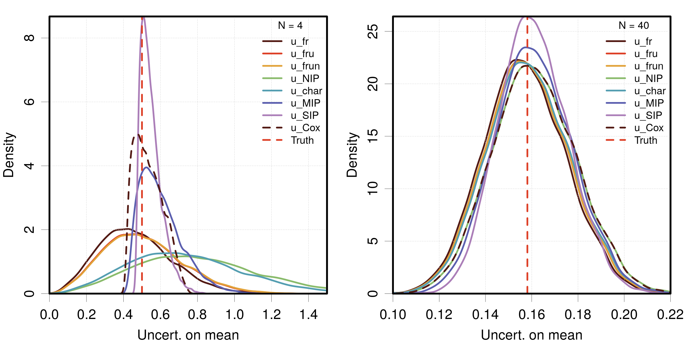
Figure 1: Density plots of uncertainty Monte Carlo samples for all uncertainty estimators and two measurement counts from a normal distribution: (left) $N=4$; (right) $N=40$.

The skewness of the distributions at small $N$ raises the problem of the choice of a location statistic for the uncertainty. We consider three of them: arithmetic mean $\left\langle u_{X}\right\rangle$; median of $u_{X}$; and root mean squared uncertainty $\sqrt{\left\langle u_{X}^{2}\right\rangle}$ (which is often used to average standard deviations). The robust Inter-Quartile Range (IQR) is used to measure the scale of the distribution. We consider also two probabilities to complement these statistics:

• the probability to get an underestimation of uncertainty

  $$P_{<}=P(u_{X}<u_{true})=\left\langle\boldsymbol{1}(u_{X}<u_{true})\right\rangle$$ (1)

  where $\boldsymbol{1}(x)$ is the indicator function. The overestimation probability is the complement to 1.

• the probability to lie within 20% of the true value

  $$P_{20}=P(u_{true}/1.2<u_{X}<1.2\times u_{true})$$ (2)

  which somewhat relaxes the difficulty of choosing a pertinent location statistic.

Table 2 and Figs.2-3 report these statistics for all uncertainty estimators.

$N$	Statistic	$u_{fr}$	$u_{fru}$	$u_{frun}$	$u_{NIP}$	$u_{char}$	$u_{MIP}$	$u_{SIP}$	$u_{Cox}$		Target
4	$\left\langle u_{X}\right\rangle$	0.463(2)	0.503(2)	0.508(2)	0.803(3)	0.738(3)	0.603(1)	0.5504(6)	0.5378(8)		0.5
	$\mathrm{med}(u_{X})$	0.446(2)	0.484(3)	0.488(3)	0.772(4)	0.709(4)	0.580(1)	0.5370(6)	0.527(1)		0.5
	$\sqrt{\left\langle u^{2}(x)\right\rangle}$	0.502(2)	0.545(2)	0.550(2)	0.870(3)	0.799(3)	0.614(1)	0.5535(6)	0.5432(8)		0.5
	IQR	0.266(3)	0.288(3)	0.291(3)	0.460(5)	0.423(5)	0.153(2)	0.0740(9)	0.120(1)		small
	$P_{<}$	0.601(5)	0.529(5)	0.522(5)	0.191(4)	0.237(4)	0.191(4)	0.191(4)	0.377(5)		0.5
	$P_{20}$	0.331(5)	0.324(5)	0.324(5)	0.178(4)	0.209(4)	0.564(5)	0.824(4)	0.772(4)		high
40	$\left\langle u_{X}\right\rangle$	0.1570(2)	0.1580(2)	0.1580(2)	0.1612(2)	0.1588(2)	0.1610(2)	0.1608(1)	0.1611(2)		0.158
	$\mathrm{med}(u_{X})$	0.1565(2)	0.1576(2)	0.1576(2)	0.1607(2)	0.1583(2)	0.1605(2)	0.1603(2)	0.1607(2)		0.158
	$\sqrt{\left\langle u^{2}(x)\right\rangle}$	0.1580(2)	0.1590(2)	0.1590(2)	0.1622(2)	0.1598(2)	0.1619(2)	0.1615(2)	0.1621(2)		0.158
	IQR	0.0241(3)	0.0243(3)	0.0243(3)	0.0248(3)	0.0244(3)	0.0229(3)	0.0204(3)	0.0248(3)		small
	$P_{<}$	0.537(5)	0.513(5)	0.513(5)	0.446(5)	0.495(5)	0.446(5)	0.446(5)	0.446(5)		0.5
	$P_{20}$	0.888(3)	0.890(3)	0.890(3)	0.888(3)	0.891(3)	0.916(3)	0.950(2)	0.889(3)		high

Table 2: Statistics for Monte Carlo samples uncertainty estimators. Except for the arithmetic mean, the estimation uncertainties (in parenthesis notation) are obtained by bootstrapping(Efron1979, ; Efron1991, ) with 5000 repeats. For each statistic, the values compatible with the target (last column) within $\pm 2\sigma$ are noted in bold. In absence of a target, the smallest or largest values are emphasized.

Let us first consider the small sample ($N=4$). It is striking that the $u_{fru}$ method gives the best estimate using the mean, while the standard $u_{fr}$ gives the best estimate using the root mean squared statistic. This is consistent with their properties, $u_{fr}$ resulting from an unbiased estimation of the variance ($u_{fr}^{2}$), while $u_{fru}$ is an unbiased estimator of standard deviation. Globally, the median does not provide an improvement over the other metrics. One can also note that for the normal distribution, $u_{frun}$ is practically indistinguishable from $u_{fru}$, a credit to Brugger’s formula.(Brugger1969, )

Based on the location statistics, all Bayesian estimators overestimate the uncertainty, albeit to a lesser extent for those based on an informative prior. Although they are considered to encode the same information level,(Cox2022, ) $u_{Cox}$ performs slightly better than $u_{SIP}$ for the three location estimators.

If one considers the inter-quartile range, $u_{SIP}$ provides the most concentrated distribution, followed by $u_{Cox}$. The largest spread is observed for $u_{NIP}$.

Among the frequentist methods, $u_{fr}$ has the highest risk to under-estimate the uncertainty($P_{<}=0.62$), while $u_{fru}$ is closer to a balanced estimation ($P_{<}=0.53$). As noted from the location statistics, all Bayesian methods tend to over-estimate the uncertainty, with probabilities between $1-P_{<}=0.79$ for $u_{NIP}$ and $1-P_{<}=0.60$ for $u_{Cox}$.

Finally, the probability to be within 20% of the true value, $P_{20}$, mirrors the IQR with the best score for $u_{SIP}$ and $u_{Cox}$ and the worst for $u_{NIP}$.

For the large sample ($N=40$), The trends noted above are still perceptible, but at a lesser level. The three location estimators give more consistent results. $u_{SIP}$ stay significantly better than the other estimators for the $P_{20}$ statistic, followed by $u_{MIP}$.

III.3 Comparison of uncertainty estimators for non-normal distributions of errors

The same statistics as above have been calculated for non-normal distributions. The results are reported in Figs. 2 for $N=4$ and Fig. 3 for $N=40$.

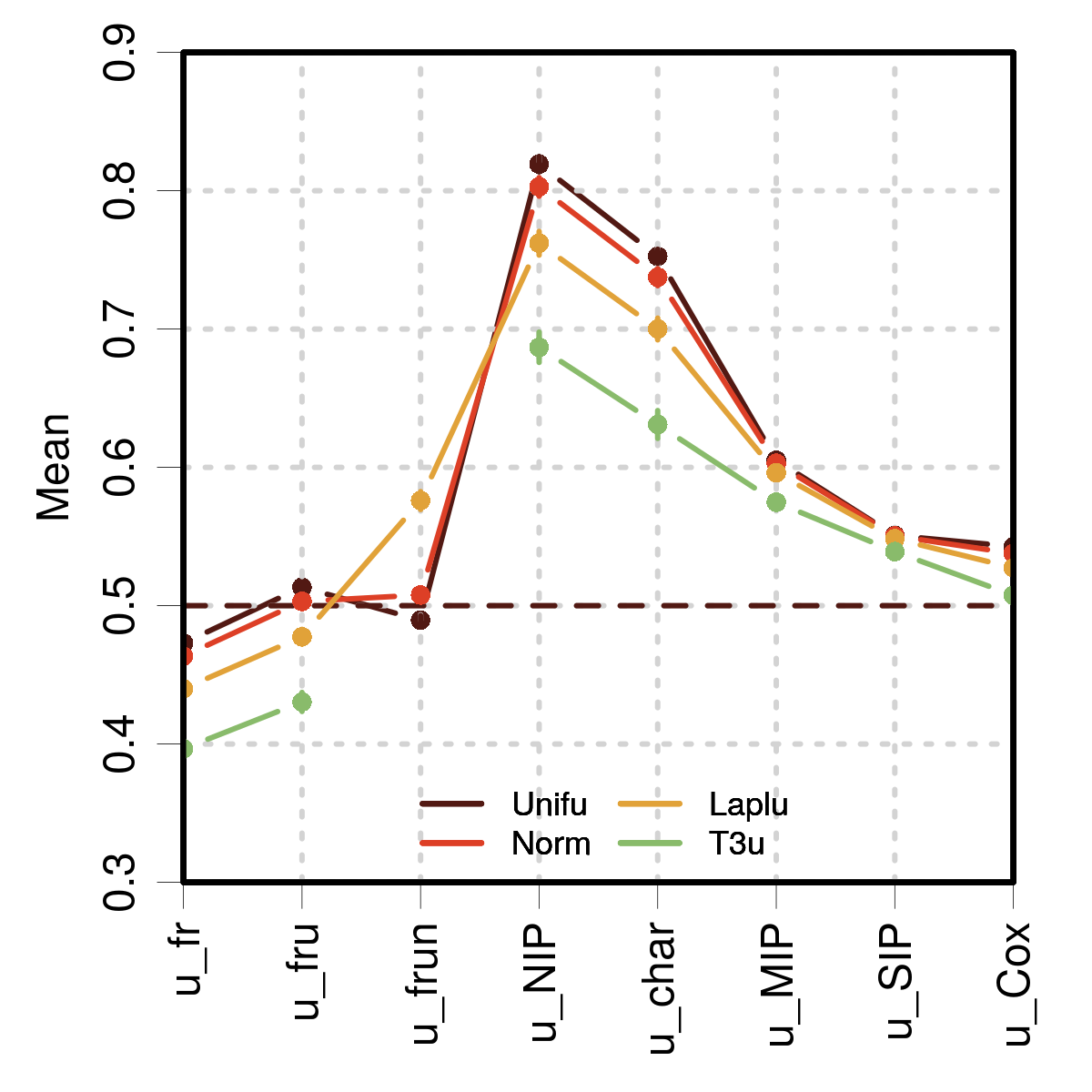
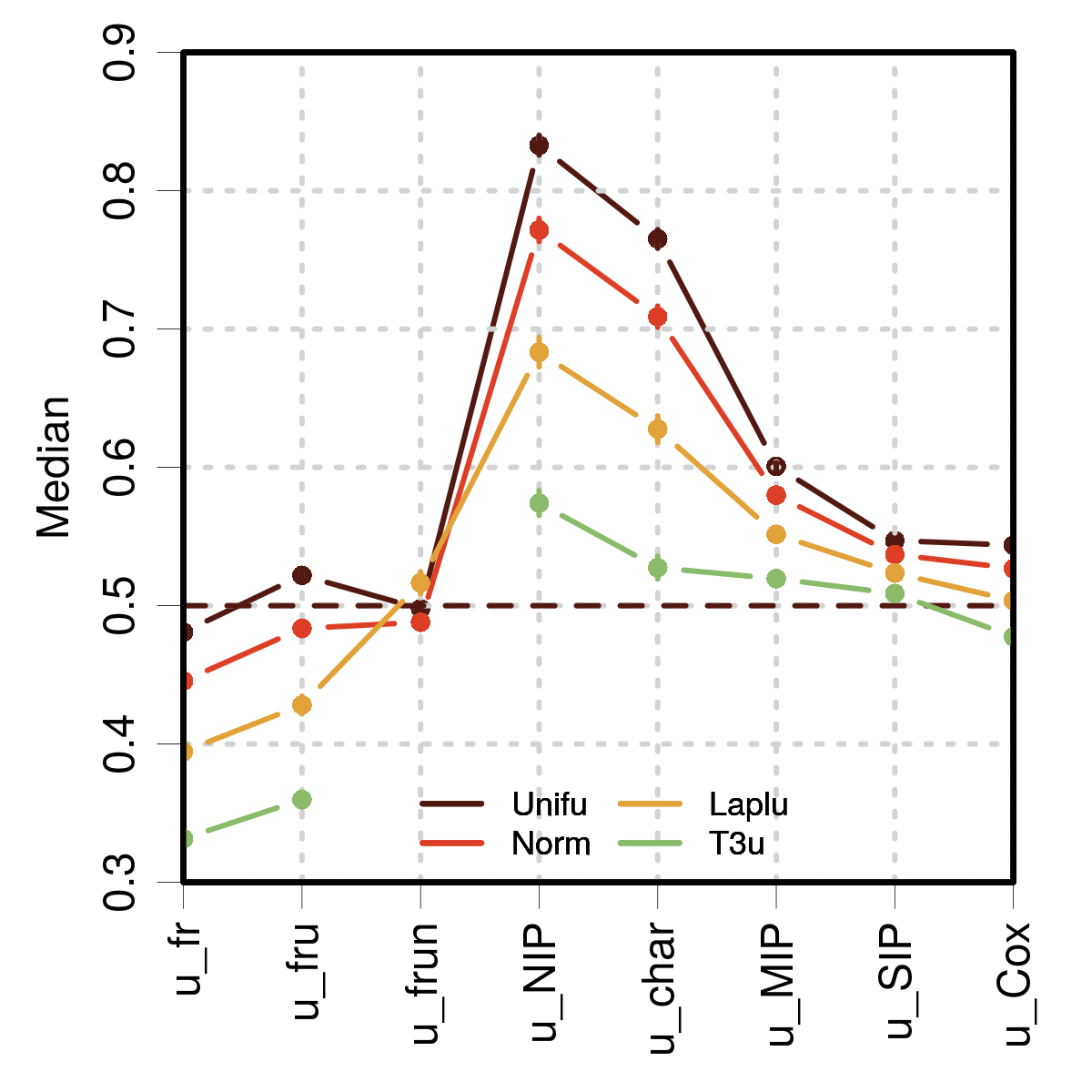
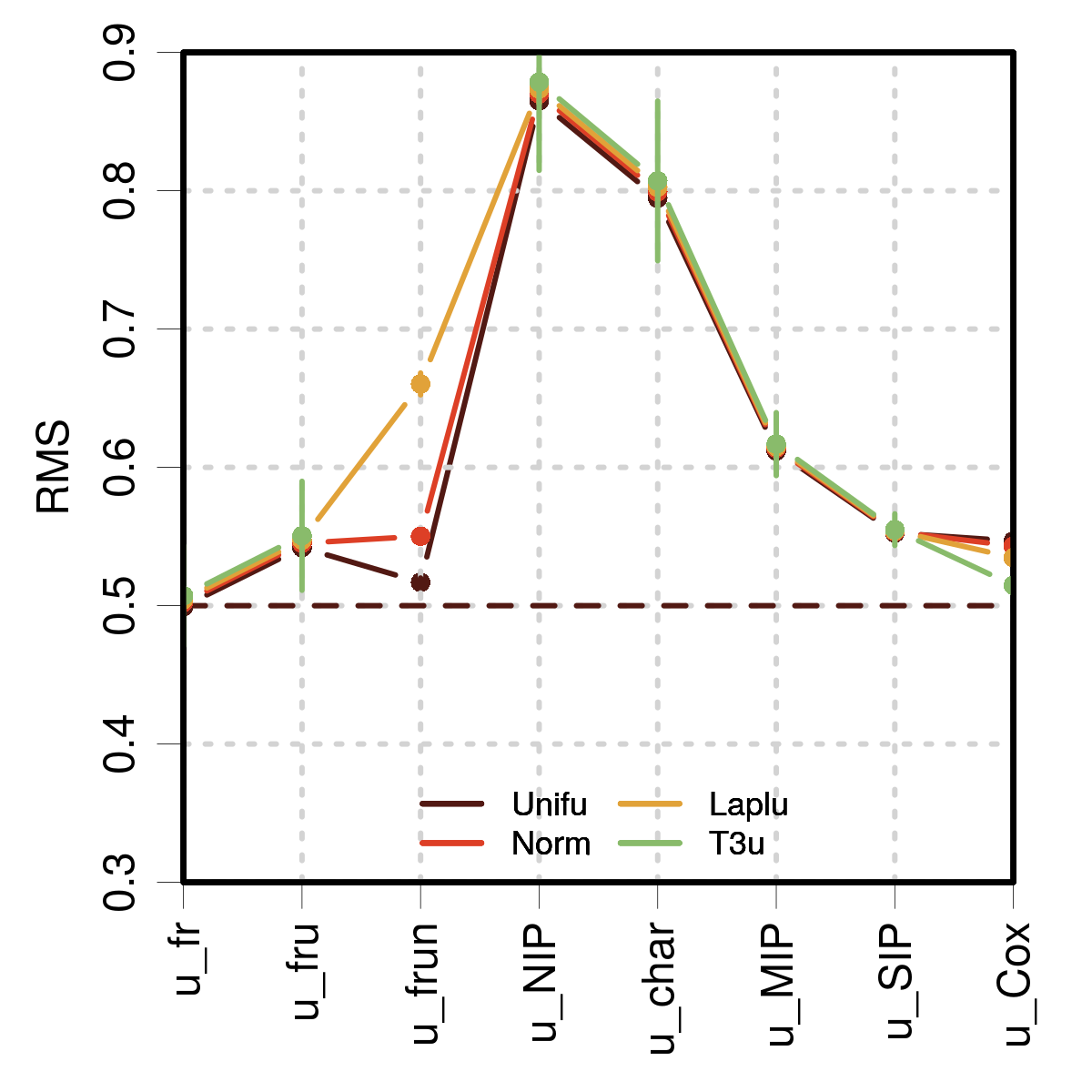
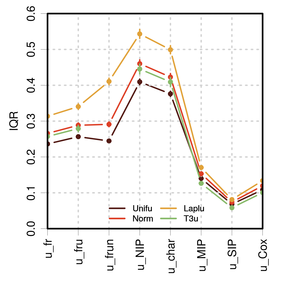
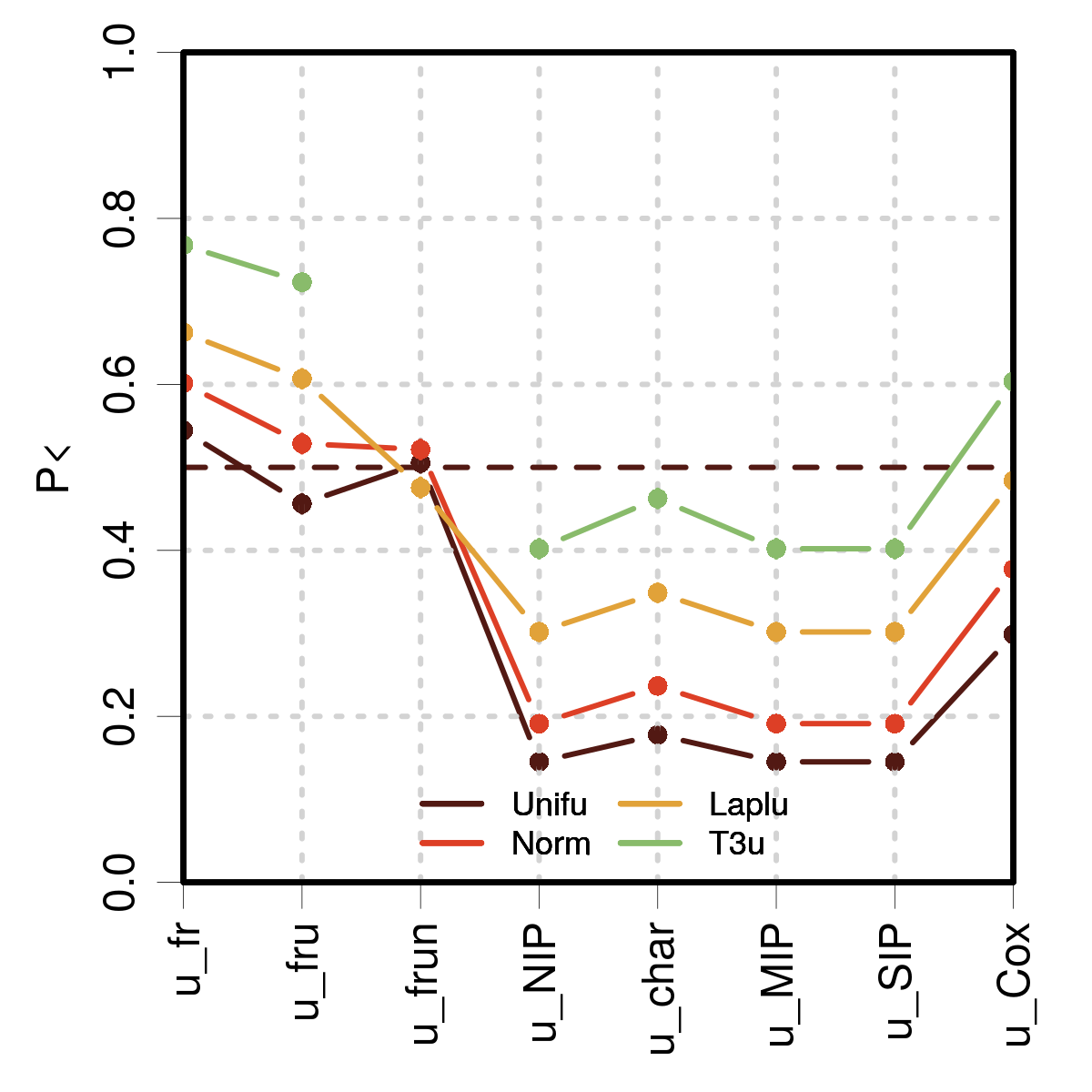
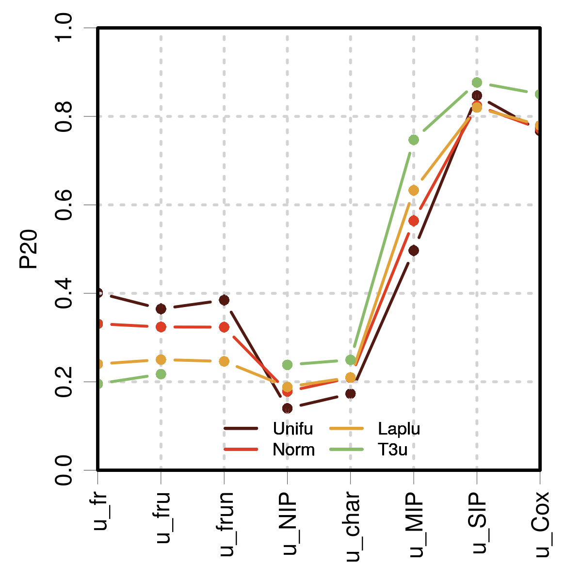
Figure 2: Statistics for $N=4$.

Several trends are clearly visible in the plots summarizing the statistics for $N=4$. For instance, the base frequentist formula $u_{fr}$ consistently underestimates the standard uncertainty, except when using the RMS estimation. It should be noted also that the RMS estimation of the mean uncertainty is the least sensitive to the non-normality of the distribution (except for $u_{frun)}$), the most sensitive one being the median. The $u_{frun}$ estimator, accounting for the excess kurtosis of the distributions seems to perform better for the median than for the mean or RMS. As a consequence, it is also the less sensitive to kurtosis when estimating $P_{<}$. However, it is not able to deal with T3u, which has an infinite kurtosis. The unbiased estimator $u_{fru}$ performs better (by design) for the normal distribution (Norm), but also for the uniform distributions (Unifu). However, it fails for the Student’s distribution (T3u), and to a lesser extent for the Laplace distribution (Laplu).

If one ignores the $u_{frun}$ estimator, one can note a systematic effect of kurtosis (all curves are parallel), and a global difficulty to deal with the T3u distribution, except for the RMS metric which presents a small offset but larger statistical uncertainties.

The performance of the Bayesian estimators depends notably on the information level introduced by the prior:

• the non-informative $u_{NIP}$, mildly informative $u_{MIP}$ and strongly informative $u_{SIP}$ priors result in consistent over-estimation of the standard uncertainty, for either Mean, Median or RMS;

• for all statistics, the $u_{char}$ estimator is closer to the target than $u_{NIP}$, although not better than the more informed Bayesian estimators;

• by comparison, the Cox prior $u_{Cox}$ provides about the same results than $u_{SIP}$, but is more sensitive to the kurtosis of the distribution for the three location statistics.

The IQR is also sensitive to kurtosis, but notably less for the Bayesian estimators based on informative priors, which provide more concentrated distributions, as noted above for the normal case. This is reflected in $P_{20}$ for which $u_{SIP}$ and $u_{Cox}$ reach levels near 0.8.

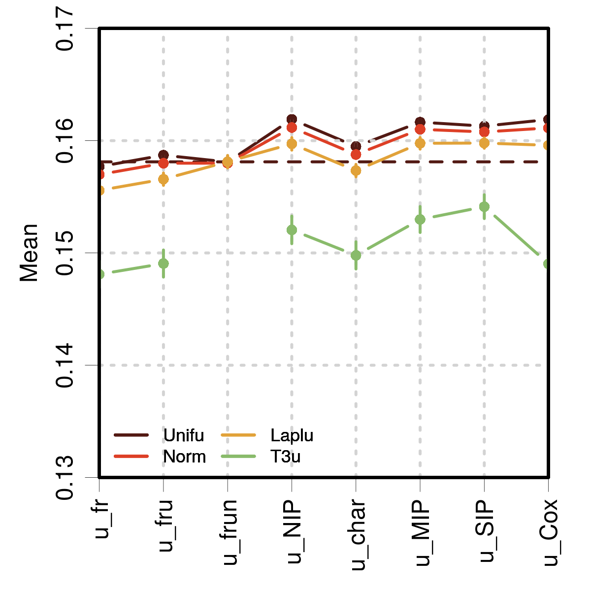
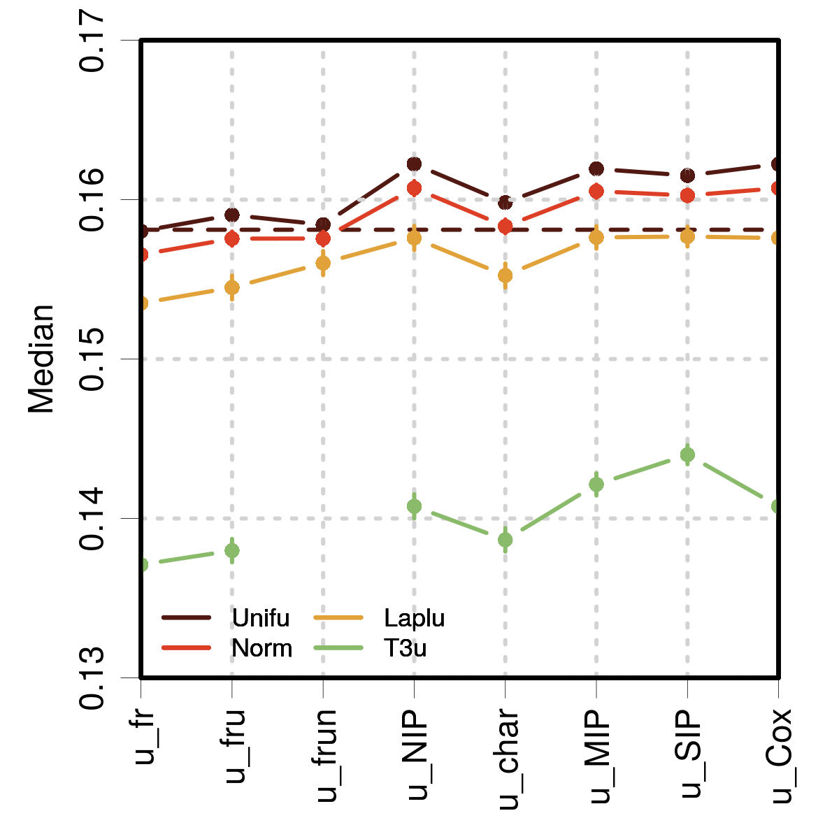
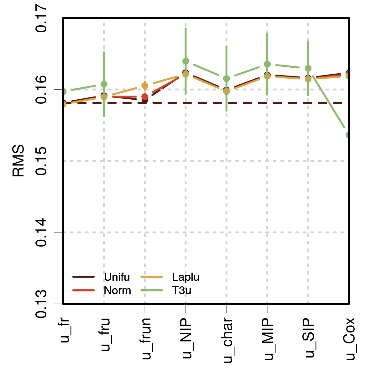
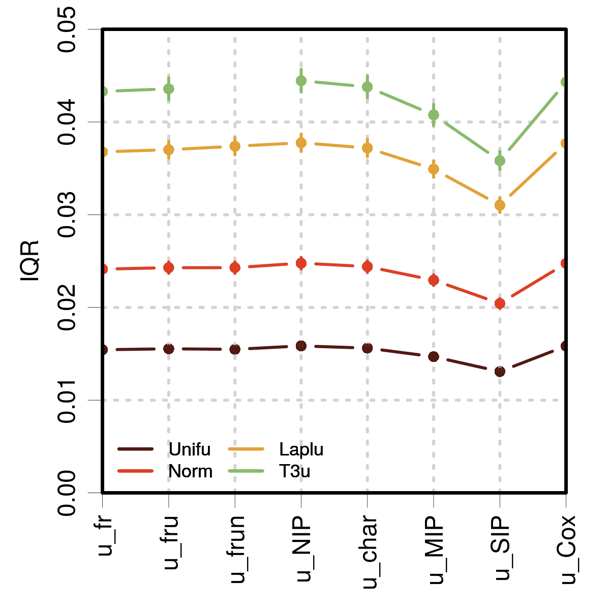
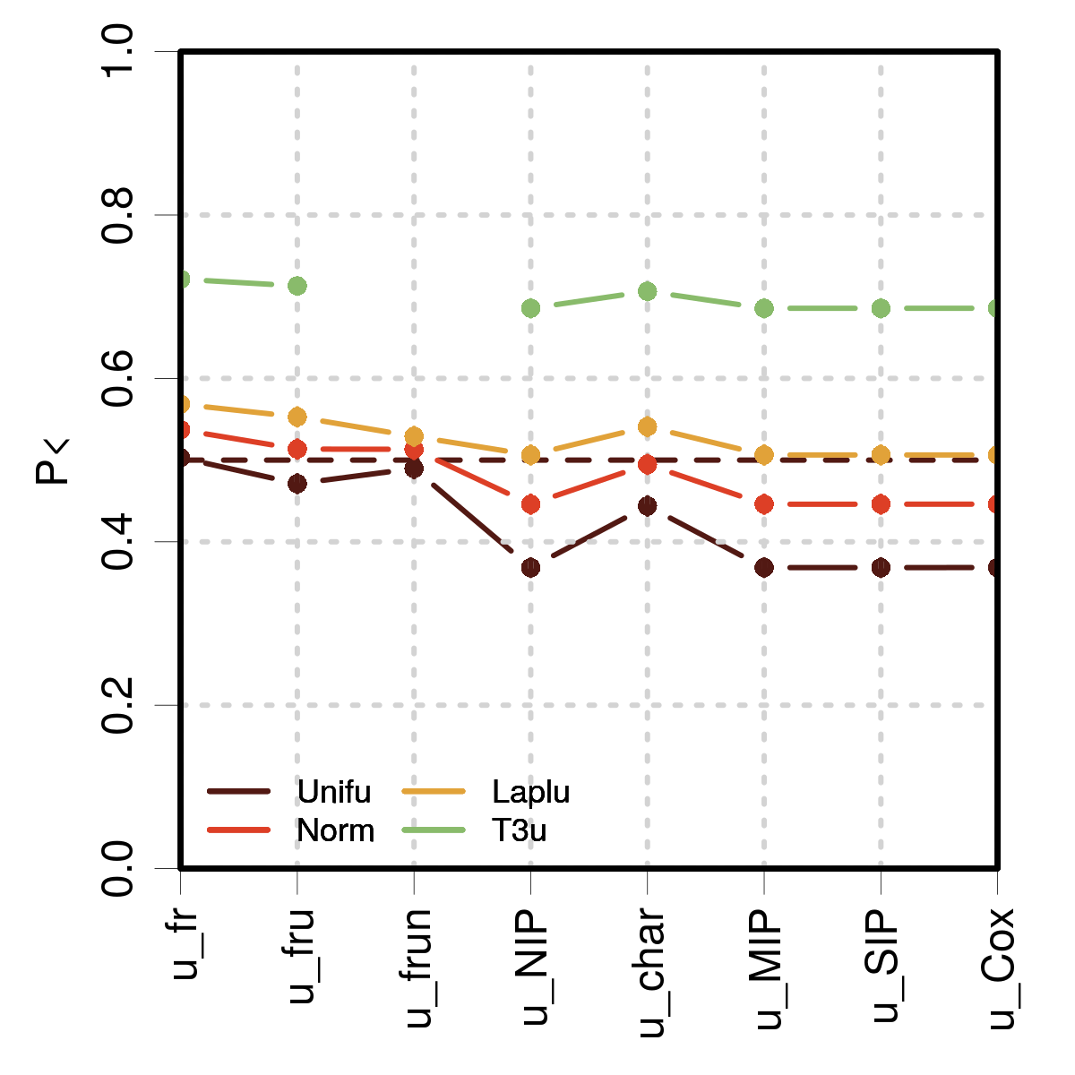
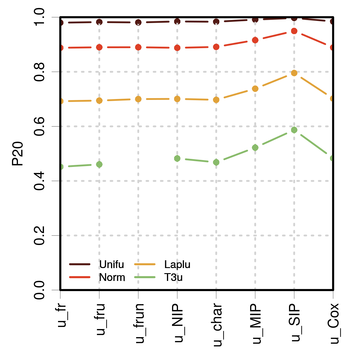
Figure 3: Statistics for $N=40$

For the larger sampling size $N=40$, the discrepancies between the estimators are strongly reduced. Concerning the location metrics, the mean is still sensitive to kurtosis, except for $u_{frun}$, the median is now the most sensitive to kurtosis, even for $u_{frun}$, and except for the T3U distribution and $u_{frun}$ estimator, the RMS metric is still the less sensitive to kurtosis.

All the Bayesian estimators are still on the side of overestimation and the impact of the prior is less sensible than for $N=4$. Surprisingly, $u_{char}$ seems to perform better than all Bayesian estimators, at least for the Unifu and Norm distributions.

IQR and $P_{20}$ are still notably sensitive to kurtosis. The best performers for all distributions are now $u_{MIP}$ and $u_{SIP}$. $u_{Cox}$ has lost the advantage it had for the small sample. Even for sets of 40 measurements, the impact of the additional information introduced by the MIP and SIP priors is non-negligible. The downside is that a wrongly designed prior might need a lot of data to be countered.

IV Conclusion

Our Monte Carlo simulations enable to dress a contrasted portrait on the mean uncertainty estimation landscape. To evaluate the performances of a comprehensive set of uncertainty estimators, several statistics were used to summarize the properties of the uncertainty distribution generated by Monte Carlo sampling. Three location statistics (mean, median, RMS), a spread statistic (IQR) and two probabilities, $P_{<}$ the probability of underestimation and $P_{20}$ the probability to lie within 20% of the true value. Several location statistics were used to account for the skewness of the uncertainty distributions, notably for small measurement samples.

For small samples, $u_{fr}$ provides closer estimates when combined with RMS, while $u_{fru}$ works better with the mean. As evoked earlier, this is consistent with the fact that $u_{fr}$ derives from an unbiased estimator of variance, while $u_{fru}$ is an unbiased estimator of standard deviation. As the GUM is by essence built on the rule of combination of variances, one might question if an unbiased estimator of standard deviation is pertinent for metrology. Additionally, we have seen that the RMS statistic is much less dependent on the kurtosis of the error distribution than the other location statistics. One might thus base the discussion on the RMS results.

In this case, $u_{fr}$ is the uncertainty estimator which gives the best estimate in the long run. By contrast, all other estimators tend to overestimate uncertainty. For instance, all tested Bayesian estimators give a notable overestimation of the uncertainty on the mean, which is better corrected by Cox’s informative prior and the strongly informative prior of O’Hagan and Cox.

A remarkable point is that the MIP, SIP and Cox estimators give an uncertainty distribution that is much more concentrated than the other ones, therefore a lesser risk of strong under- or over- estimation. This comes however with a caveat about the necessity of a good prior parameterization.

Globally, there is a significant gain in using the Bayesian estimators with informative priors. For small measurement sets, they provide more conservative uncertainty values, but also a very good probability to lie within some tight interval around the true value. On all aspects, the estimator based on a non-informative prior $u_{NIP}$ does not seem to be a good choice, even worse than the frequentist formulas.

Finally, one should be aware that all estimators, even the unbiased ones, are at some level sensitive to the shape of the error distribution, and seem to be at pain for distributions with strong positive excess kurtosis [Laplace or Student’s-t($\nu=3$)].

Data availability statement

The R code that enables to reproduce the figures and tables of this study is openly available at the following URL: https://github.com/ppernot/2022_SampleMean, or in Zenodo at https://doi.org/10.5281/zenodo.7063942.

References

- (1) BIPM, IEC, IFCC, ILAC, ISO, IUPAC, IUPAP, and OIML. Evaluation of measurement data - Guide to the expression of uncertainty in measurement (GUM). Technical Report 100:2008, Joint Committee for Guides in Metrology, JCGM, 2008. URL: http://www.bipm.org/utils/common/documents/jcgm/JCGM_100_2008_F.pdf.
- (2) BIPM, IEC, IFCC, ILAC, ISO, IUPAC, IUPAP, and OIML. Evaluation of measurement data - Supplement 1 to the "Guide to the expression of uncertainty in measurement" - Propagation of distributions using a Monte Carlo method. Technical Report 101:2008, Joint Committee for Guides in Metrology, JCGM, 2008. URL: http://www.bipm.org/utils/common/documents/jcgm/JCGM_101_2008_E.pdf.
- (3) R. Kacker and A. Jones. On use of bayesian statistics to make the Guide to the Expression of Uncertainty in Measurement consistent. Metrologia, 40:235–248, 2003.
- (4) H. Huang. Comparison of three approaches for computing measurement uncertainties. Measurement, 163:107923, 2020.
- (5) M. Cox and K. Shirono. Informative bayesian type a uncertainty evaluation, especially applicable to a small number of observations. Metrologia, 54:642–652, 2017.
- (6) A. O’Hagan and M. Cox. Simple informative prior distributions for metrology. Working document, November 2021. URL: http://www.tonyohagan.co.uk/academic/pdf/Simple_Priors.pdf.
- (7) M. Cox and A. O’Hagan. Meaningful expression of uncertainty in measurement. Accredit Qual Assur, 27:19–37, 2022.
- (8) D. C. Bailey. Not Normal: the uncertainties of scientific measurements. R. Soc. Open Sci., 4:160600, 2017.
- (9) R Core Team. R: A Language and Environment for Statistical Computing. R Foundation for Statistical Computing, Vienna, Austria, 2019. URL: http://www.R-project.org/.
- (10) R. M. Brugger. A note on unbiased estimation of the standard deviation. Amer. Statist., 23(4):32–32, 1969. URL: https://www.tandfonline.com/doi/abs/10.1080/00031305.1969.10481865.
- (11) Wikipedia Contributors. Unbiased estimation of standard deviation - Wikipedia, 2022. [Online; accessed 11. Jul. 2022]. URL: https://en.wikipedia.org/w/index.php?title=Unbiased_estimation_of_standard_deviation&oldid=1071100403.
- (12) B. Efron. Bootstrap Methods: Another Look at the Jackknife. Ann. Stat., 7(1):1–26, January 1979.
- (13) B. Efron and R. Tibshirani. Statistical data analysis in the computer age. Science, 253:390–395, 1991.