RASR: Risk-Averse Soft-Robust MDPs
with EVaR and Entropic Risk

Abstract

Prior work on safe Reinforcement Learning (RL) has studied risk-aversion to randomness in dynamics (aleatory) and to model uncertainty (epistemic) in isolation. We propose and analyze a new framework to jointly model the risk associated with epistemic and aleatory uncertainties in finite-horizon and discounted infinite-horizon MDPs. We call this framework that combines Risk-Averse and Soft-Robust methods RASR. We show that when the risk-aversion is defined using either EVaR or the entropic risk, the optimal policy in RASR can be computed efficiently using a new dynamic program formulation with a time-dependent risk level. As a result, the optimal risk-averse policies are deterministic but time-dependent, even in the infinite-horizon discounted setting. We also show that particular RASR objectives reduce to risk-averse RL with mean posterior transition probabilities. Our empirical results show that our new algorithms consistently mitigate uncertainty as measured by EVaR and other standard risk measures.

1 Introduction

A major concern in high-stakes applications of reinforcement learning (RL), such as those in healthcare and finance, is to quantify the risk associated with the variability of returns. This variability is a form of aleatory uncertainty that arises from the inherent randomness in system dynamics. Since the risk of random returns cannot be captured by the standard expected objective, convex risk measures have emerged as perhaps the most popular tools to quantify this risk in RL and beyond. They are sufficiently general to capture a wide range of stakeholder preferences and are more computationally convenient than many other alternatives Follmer and Schied (2004). Conditional value-at-risk (CVaR), entropic value-at-risk (EVaR) Ahmadi-Javid (2012); Föllmer and Knispel (2011), and entropic risk measure (ERM) Follmer and Schied (2004) are common examples of convex risk measures.

The goal in robust Markov decision process (MDP) is to mitigate performance loss due to uncertainty in modeling the system dynamics Grand-Clement and Kroer (2021); Iyengar (2005); Ho et al. (2021). This uncertainty, often caused by limited or noisy data, is a form of epistemic uncertainty. Soft-robust formulations refine robust optimization by assuming a Bayesian distribution over plausible models (of the system dynamics) and then quantify the risk of model errors using convex risk measures Derman et al. (2018); Lobo et al. (2021). These formulations have close connections to distributional robustness Xu and Mannor (2012). While being risk-averse to epistemic uncertainty, existing soft-robust RL formulations are risk-neutral when it comes to the aleatory uncertainty that arises from the randomness in the system dynamics. This combination of risk-aversion to epistemic uncertainty with risk-neutrality to aleatory uncertainty can be problematic from the modeling perspective Chow et al. (2018), and as we show below, may introduce unnecessary computational complexity.

The overarching objective of our work is to compute policies for MDPs that jointly mitigate the risk associated with epistemic (model) and aleatory (random dynamics) uncertainties. We call this objective RASR as it combines Risk Averse (aleatory) and Soft-Robust (epistemic) methods. This is in contrast to the existing soft-robust MDP algorithms that are risk-neutral to the aleatory uncertainty. In this paper, we study RASR with two popular risk measures: ERM and EVaR.

As our first contribution, in Section 3, we introduce our RASR-ERM framework and propose new dynamic programming algorithms and analysis for it. ERM is unique among law-invariant risk measures in being dynamically consistent Kupper and Schachermayer (2006), which makes it compatible with dynamic programming (DP). Unfortunately, ERM is not positively homogeneous, which makes it incompatible with the use of discount factors. As a result, ERM has only been solved exactly in average-reward MDPs Borkar and Meyn (2002) and undiscounted stochastic programs Dowson et al. (2021). Our main innovation is to use time-dependent risk levels to precisely solve ERM in discounted finite-horizon MDPs and to employ new bounds to tightly approximate it in discounted infinite-horizon MDPs (Section 3.2). We build on the DP decomposition of the RASR-ERM objective to show that there exists an optimal value function and (surprisingly) a deterministic Markov optimal policy for this problem. This is unusual because most other risk-averse formulations require randomized optimal policies. We also show that under an assumption of a dynamic model of epistemic uncertainty Derman et al. (2018); Eriksson and Dimitrakakis (2020), the RASR-ERM objective reduces to a risk-averse MDP with the mean posterior transition model (Section 3.1).

As our second contribution, we formulate and study the RASR-EVaR framework in Section 4. Although ERM is computationally convenient, it is often an impractical method to measure risk since the result is scale-dependent. EVaR is preferable to ERM because it is coherent, positively-homogenous, interpretable, and comparable with VaR and CVaR. However, EVaR is not dynamically consistent and cannot be directly optimized using a DP. Our main contribution here is to reduce the RASR-EVaR optimization to multiple RASR-ERM problems that each can be solved by DP. Our theoretical analysis shows that the RASR-EVaR properties mirror those for RASR-ERM and that the proposed algorithm can compute a solution arbitrarily close to the optimum. We empirically evaluate our RASR algorithms in Section 5 and show their benefits over prior robust, soft-robust, and risk-averse MDP algorithms. Finally, in Section 6, we position our RASR framework in the context of the literature on soft-robust and risk-averse MDPs.

2 Preliminaries

We assume the decision problem can be formulated as an MDP, defined by the tuple $(\mathcal{S},\mathcal{A},r,p,s_{0},\gamma)$. The state and action sets $\mathcal{S}$ and $\mathcal{A}$ are finite with cardinality $S$ and $A$. The reward function $r\colon\mathcal{S}\times\mathcal{A}\to\mathbb{R}$ represents the reward received in each state after taking an action. We use $\triangle r=\max_{s\in\mathcal{S},a\in\mathcal{A}}r(s,a)-\min_{s\in\mathcal{S},a\in\mathcal{A}}r(s,a)$ to refer to the span semi-norm of the rewards. The transition probabilities are denoted as $p\colon\mathcal{S}\times\mathcal{A}\to\Delta^{S}$, where $\Delta^{S}$ is the probability simplex in $\mathbb{R}^{S}$. The initial state is denoted by $s_{0}\in\mathcal{S}$. Finally, $\gamma\in(0,1]$ is the discount factor. We assume a fixed horizon $T\in\mathbb{N}^{+}\cup\{\infty\}$ with $T=\infty$ indicating an infinite-horizon objective. While a discounted finite-horizon objective is uncommon in practice, it serves us as an intermediate step when analyzing the infinite-horizon objective.

The most-general solution to an MDP is a randomized history-dependent policy that at each time step prescribes a distribution over actions as a function of the history up to that step Puterman (2005). A randomized Markov policy depends only on the time step $t$ and current state $s_{t}$ as $\pi=(\pi_{t})_{t=0}^{T-1}$, where $\pi_{t}\colon\mathcal{S}\to\Delta^{A}$. A policy $\pi$ is stationary when it is time-independent (all $\pi_{t}$’s are equal), in which case we omit the time subscript. We denote by $\Pi_{MR}$ and $\Pi_{SR}$, the sets of Markov and stationary randomized policies, and by $\Pi_{MD}$ and $\Pi_{SD}$, the corresponding sets of deterministic policies. The set of history-dependent randomized policies is denoted by $\Pi_{HR}$

We define $\mathfrak{R}_{T}^{\pi}$, the random variable of the return of a policy $\pi$ after $T$ time steps as

$$\mathfrak{R}_{T}^{\pi}\;=\;\sum_{t=0}^{T-1}\gamma^{t}\cdot R_{t}^{\pi}=\sum_{t=0}^{T-1}\gamma^{t}\cdot r(S_{t}^{\pi},A^{\pi}_{t})\leavevmode\nobreak\ ,$$ (1)

where $S_{t}^{\pi}$, $A_{t}^{\pi}\sim\pi_{t}(\cdot|S_{t}^{\pi})$, and $R_{t}^{\pi}$ are the random variables of state visited, action taken, and reward received respectively at time $t\in 0,\dots,T$, when following policy $\pi$. The objective in the standard risk-neutral MDP is to maximize the expectation of the return random variable,

$$\max_{\pi\in\Pi_{{MR}}}\,\mathbb{E}\big{[}\mathfrak{R}^{\pi}_{T}\big{]}\leavevmode\nobreak\ .$$ (2)

In finite-horizon MDPs, $T<\infty$ and (usually) $\gamma=1$. In infinite-horizon discounted MDPs, we use $T=\infty$ (as a shorthand for $T\rightarrow\infty$) and restrict the discount factor to $\gamma\in(0,1)$. It is known that the finite and infinite horizon discounted settings have optimal policies in $\Pi_{MD}$ and $\Pi_{SD}$, respectively.

Risk-averse MDP

A risk measure $\psi\colon\mathbb{X}\to\mathbb{R}$ assigns a scalar risk value to a random variable $X\in\mathbb{X}$, where $\mathbb{X}$ denotes the set of real-valued random variables. Convex risk measures are an axiomatic generalization of the expectation operator $\mathbb{E}[\cdot]$ that capture a wide range of risk-aversion preferences Föllmer and Schied (2002); Frittelli and Rosazza Gianin (2002). We describe coherent and convex risk measures, and summarize their properties that are desirable in studying risk-averse MDPs in Section E. The objective in risk-averse MDP is defined by replacing the expectation in (2) with an appropriate risk measure

$$\max_{\pi\in\Pi_{HR}}\,\psi\big{[}\mathfrak{R}_{T}^{\pi}\big{]}.$$ (3)

Soft-robust MDP

The soft-robust setting makes the Bayesian assumption that the transition model $P$ is a random variable with a distribution that can be computed, for instance, using Bayesian inference Derman et al. (2018); Eriksson and Dimitrakakis (2020); Lobo et al. (2021). In this paper, we assume a dynamic model of uncertainty Derman et al. (2018); Eriksson and Dimitrakakis (2020). In the dynamic model, the transition probability is not only unknown, but can also change during the execution. This is in contrast to the static model Delage and Mannor (2009); Lobo et al. (2021), in which it is uncertain but does not change throughout an episode. We target dynamic uncertainty because it is easier to optimize and our results lay down the foundations necessary to tackle static models in future. In the dynamic model, the transition probability is defined as $P=(P_{t})_{t=0}^{T-1}$, where each model $P_{t}\colon\Omega\to(\Delta^{S})^{\mathcal{S}\times\mathcal{A}}$ is a random variable that represent the uncertain transition functions for some finite set of possible models $\Omega$. The uncertain models are distributed independently across time as $P_{t}\sim f_{t}$, and $f_{t}\in\Delta^{\Omega},\,t=0,\dots,T-1$ are derived from Bayesian inference methods. Note that the upper-case $P$ is a random variable that represents an uncertain transition function in a soft-robust MDP, whereas the lower-case $p$ is used to denote a known transition function in an MDP.

Prior work on soft-robust RL (e.g., Derman et al. (2018); Eriksson and Dimitrakakis (2020); Lobo et al. (2021)) has focused on the following objective:

$$\max_{\pi\in\Pi_{HR}}\;\psi\Big{[}\mathop{\mathbb{E}}\big{[}\mathfrak{R}_{T}^{\pi}\mid P\big{]}\Big{]}.$$ (4)

In (4), the risk measure $\psi$ is applied only to the epistemic uncertainty over $P$, and the optimization is risk-neutral (uses $\mathbb{E}[\cdot]$) to the randomness in $\mathfrak{R}_{T}^{\pi}\mid P$ (aleatory uncertainty). For some particular choices of $\psi$, the optimization in (4) reduces to a distributionally-robust MDP Xu and Mannor (2012); Grand-Clement and Kroer (2021); Lobo et al. (2021).

RASR

Our RASR formulation, introduced formally below, takes into account both the epistemic uncertainty in the transition model $P$ and the aleatory uncertainty in $\mathfrak{R}_{T}^{\pi}\mid P$, and optimizes the objective

$$\max_{\pi\in\Pi_{HR}}\;\psi\Big{[}\psi\big{[}\mathfrak{R}_{T}^{\pi}\mid P\big{]}\Big{]}.$$ (5)

Given the well-known equivalence between coherent risk measures and robustness (e.g., Osogami (2012)), it is tempting to conclude that the combination of risk and soft-robustness in (5) reduces to a robust MDP. Alas, this is false for virtually all reasonable choices of the risk measure $\psi$. The risk-robustness equivalence is only known for risk-averse formulations in (4) that admit a dynamic program formulation, that is when $\psi$ is dynamically consistent. As we discuss above, most practical risk measures—such as VaR, CVaR, EVaR and others—are not dynamically consistent Iancu et al. (2015), and therefore, neither (3) nor (5) readily reduce to a robust MDP.

Risk Measures

We study two convex risk measures in our RASR formulation: entropic risk measure (ERM) andu entropic value-at-risk (EVaR). ERM with a risk-aversion parameter $\alpha\in\mathbb{R}_{+}\cup\{\infty\}$, for a random variable $X\in\mathbb{X}$, is defined as Follmer and Schied (2004)

$$\operatorname{ERM}^{\alpha}[X]=-\alpha^{-1}\cdot\log\Bigl{(}\mathbb{E}\left[e^{-\alpha\cdot X}\right]\Bigr{)}.$$ (6)

For the risk level $\alpha=0$, ERM of a random variable equals to its expectation, $\operatorname{ERM}^{0}[X]=\lim_{\alpha\to 0^{+}}\operatorname{ERM}^{\alpha}[X]=\mathbb{E}[X].$ Similarly, $\operatorname{ERM}^{\infty}[X]=\operatorname{ess}\inf[X]$ is the minimum value of $X$. Note that we use an ERM definition in (6) that is meant to be maximized. ERM definitions designed to be minimized lack the leading negative sign Föllmer and Knispel (2011).

ERM is the only law-invariant convex risk measure that is dynamically-consistent Kupper and Schachermayer (2006) (see Section E.5). This is an important property for a risk measure in multi-stage decision problems, because it allows defining a dynamic program (DP) for the risk measure and optimizing it. The following theorem is crucial for deriving our results. It has been proved in earlier work, but we report its proof in Section A for completeness.

Theorem 1 (Tower Property).

Any two random variables $X_{1},X_{2}\in\mathbb{X}$ satisfy that

$$\operatorname{ERM}^{\alpha}[X_{1}]\;=\;\operatorname{ERM}^{\alpha}\big{[}\operatorname{ERM}^{\alpha}[X_{1}\mid X_{2}]\big{]}\leavevmode\nobreak\ .$$

Note that the tower property also holds for the expectation operator $\mathbb{E}[\cdot]$, but is violated by most common risk measures, including VaR, CVaR, and EVaR. Despite its many nice features, ERM also has several undesirable properties. It is not positively-homogeneous: $\operatorname{ERM}^{\alpha}[c\cdot X]\neq c\cdot\operatorname{ERM}^{\alpha}[X]$, for $c\geq 0$, which means that $\operatorname{ERM}^{\alpha}[X]$ does not scale linearly with $X$. Moreover, ERM is difficult to interpret and its risk level $\alpha$ is not readily comparable to the risk levels of VaR and CVaR.

EVaR was proposed to address some of the shortcomings of ERM. EVaR with confidence parameter $\beta\in[0,1)$, for a random variable $X\in\mathbb{X}$, is defined as Föllmer and Knispel (2011); Ahmadi-Javid (2012)

$$\operatorname{EVaR}^{\beta}[X]\;=\;\sup_{\alpha>0}\,\left(\operatorname{ERM}^{\alpha}[X]+\alpha^{-1}\cdot\log(1-\beta)\right).$$ (7)

The supremum in (7) is achieved for any $X$ with a bounded support. Although EVaR is not dynamically consistent, we show in Section 4 that it can be optimized using a DP by representing it in terms of ERM. Unlike ERM, EVaR is positively-homogeneous, and thus, coherent, which makes its riskiness independent of the scale of the random variable. Moreover, the meaning of its risk level $\beta$ is consistent with those used in VaR and CVaR, with $\operatorname{EVaR}^{0}[X]=\mathbb{E}[X]$ and $\lim_{\beta\rightarrow 1}\operatorname{EVaR}^{\beta}[X]=\operatorname{ess}\inf[X]$. Finally, since $\operatorname{EVaR}^{\beta}[X]\leq\operatorname{CVaR}^{\beta}[X]\leq\operatorname{VaR}^{\beta}[X]$, EVaR can be interpreted as the tightest conservative approximation that can be obtained from the Chernoff inequality for VaR and CVaR Ahmadi-Javid (2012).

3 RASR-ERM Framework

In this section, we describe our RASR formulation with the entropic risk measure (ERM), which we refer to as RASR-ERM. In particular, we show that the RASR-ERM objective can be optimized using a novel DP formulation with time-dependent risk. We also establish fundamental properties for the optimal policies of this formulation. The proofs of all the results of this section are in Section B.

We adopt the soft-robust RL model with dynamic uncertainty. Thus, we assume that the transition model $P=(P_{t})_{t=0}^{T-1}$ is a collection of random variables as described in Section 2. Following the RASR objective in (5), the RASR-ERM objective is to maximize the ERM of the total return with both model uncertainty (epistemic) and random dynamics (aleatory), and is formally defined as

$$\max_{\pi\in\Pi_{HR}}\operatorname{ERM}^{\alpha}\left[\mathfrak{R}_{T}^{\pi}\right]\;=\;\max_{\pi\in\Pi_{HR}}\operatorname{ERM}^{\alpha}\big{[}\operatorname{ERM}^{\alpha}\left[\mathfrak{R}_{T}^{\pi}\mid P\right]\big{]}.$$ (8)

The ERM on the LHS of (8) applies to epistemic and aleatory uncertainties simultaneously and equals to the nested ERM formula on the RHS by Theorem 1. Compared with (3), the optimization in (8) involves risk-aversion to the model (epistemic) uncertainty. Compared to (4), the aleatory uncertainty in the return random variable, $\mathfrak{R}_{T}^{\pi}\mid P$, is modeled by the same risk measure (ERM in place of $\mathbb{E}[\cdot]$) as the one used to model the risk associated with the epistemic (model) uncertainty. We refer to an optimal solution to (8) as an optimal policy $\pi^{\star}=(\pi_{t}^{\star})_{t=0}^{T-1}$. To simplify the exposition, we restrict our attention in (8) to Markov deterministic policies, because the DP formulation that we derive in Section 3.1 shows that history-dependent or randomized policies offer no advantage in RASR-ERM.

3.1 Dynamic Program Formulation for RASR-ERM

Before deriving DP equations for the value function in RASR-ERM, we show a simple, but critical, property of ERM. While ERM is known not to be positively homogeneous, the following new result shows that it has a similar property, if we allow for a change in the risk level.

Theorem 2 (Positive Quasi-homogeneity).

Let $X\in\mathbb{X}$ be a random variable. Then, for any constant $c\geq 0$ and $\alpha\geq 0$, we have that

$$\operatorname{ERM}^{\alpha}[c\cdot X]\;=\;c\cdot\operatorname{ERM}^{\alpha\cdot c}[X]\;.$$

With the two ERM properties stated in Theorems 1 and 2, we are now ready to propose the value function and DP (Bellman) equations for RASR-ERM. The value function for a policy $\pi$ is the collection $v^{\pi}=(v^{\pi}_{t})_{t=0}^{T}$, where $v^{\pi}_{t}:\mathcal{S}\rightarrow\mathbb{R}$ is the value at time step $t$ and is defined as

$$v^{\pi}_{t}(s)\;=\;\operatorname{ERM}^{\alpha\cdot\gamma^{t}}\left[\sum_{t^{\prime}=t}^{T-1}\gamma^{t^{\prime}-t}\cdot R^{\pi}_{t^{\prime}}\mid S_{t}=s\right],\quad\forall s\in\mathcal{S}.$$ (9)

We define the optimal value function $v^{\star}=(v^{\star}_{t})_{t=0}^{T}$ as the value function of an optimal policy $\pi^{\star}$, $v^{\star}=v^{\pi^{\star}}$, and let the terminal value function equal to $v_{T}^{\pi}(s)=0$. The definition of $v^{\pi}$ with a time-dependent risk aversion parameter is designed specifically to ensure that $v_{0}^{\pi}(s_{0})=\operatorname{ERM}^{\alpha}\left[\mathfrak{R}_{T}^{\pi}\right]$ and that $v^{\pi}$ can be computed using dynamic programming equations, as we show below.

The dependence of risk level on the time step $t$ in the value function definition (9) is quite important in deriving our DP formulation for RASR-ERM below. As time progresses, the risk level $\alpha\cdot\gamma^{t}$ decreases monotonically, and the value function in (9) becomes less risk-averse. Recall that in the risk-neutral setting, the risk level is $\alpha=0$ and $\operatorname{ERM}^{0}[X]=\mathbb{E}[X]$. Similarly, when we set $\alpha=0$ in (9), the value function becomes independent of $t$. Then, if there is no epistemic uncertainty, the function in (9) reduces to the standard MDP value function.

The next result states the Bellman equations for RASR-ERM value functions.

Theorem 3 (Bellman Equations).

For any policy $\pi\in\Pi_{MR}$, its value function $v^{\pi}=(v_{t}^{\pi})_{t=0}^{T}$ defined in (9) is the unique solution to the following system of equations:

$$v_{t}^{\pi}(s)\;=\;\operatorname{ERM}^{\alpha\cdot\gamma^{t}}\left[r(s,A)+\gamma\cdot v_{t+1}^{\pi}(S^{\prime})\right],\quad\forall s\in\mathcal{S},\;\forall t\in\{0,\ldots,T-1\},$$ (10)

where $A\sim\pi_{t}(\cdot|s)$, $S^{\prime}\sim\bar{p}_{t}(\cdot|s,A)$, $\bar{p}_{t}(s^{\prime}|s,a)=\mathbb{E}[P_{t}(s^{\prime}|s,a)]$, and $v_{T}^{\pi}(s)=0$ for each $s\in\mathcal{S}$. Moreover, the optimal value function $v^{\star}=(v^{\star}_{t})_{t=0}^{T}$ (defined previously) satisfies $v_{T}^{\star}(s)=0$ and is the unique solution to

$$v^{\star}_{t}(s)\;=\;\max_{a\in\mathcal{A}}\,\operatorname{ERM}^{\alpha\cdot\gamma^{t}}\left[r(s,a)+\gamma\cdot v_{t+1}^{\star}(S^{\prime})\right],\quad\forall s\in\mathcal{S},\;S^{\prime}\sim\bar{p}_{t}(\cdot|s,a).$$ (11)

Note that the ERM operator in (10) and (11) applies to the random variables $A$ and $S^{\prime}$.

Theorem 3 suggests several new important and surprising properties for the RASR-ERM objective (8). The first property that follows from the DP equations in Theorem 3 is that the RASR-ERM objective (8) is equivalent to a risk-averse RL problem with the mean posterior transition model $\bar{p}$ defined in Theorem 3.

Corollary 4.

The return for each policy $\pi\in\Pi_{MR}$ satisfies that

$$\operatorname{ERM}^{\alpha}\big{[}\operatorname{ERM}^{\alpha}[\mathfrak{R}_{T}^{\pi}\mid P]\big{]}=\operatorname{ERM}^{\alpha}\left[\mathfrak{R}_{T}^{\pi}\mid P=\bar{p}\right],$$

where $\bar{p}=(\bar{p}_{t})_{t=0}^{T-1}$ is defined as in Theorem 3.

The second important result that follows from Theorem 3 is that there exists an optimal Markov (as opposed to history-dependent) deterministic policy for the RASR-ERM objective (8), which is greedy w.r.t. the optimal value function $v^{\star}$ defined by (11). However, unlike in risk-neutral MDPs Puterman (2005), the optimal RASR-ERM policy may be time-dependent even when the horizon $T$ is large or inifnite.

Theorem 5.

There exists a Markov deterministic optimal policy $\pi^{\star}=(\pi_{t}^{\star})_{t=0}^{T-1}\in\Pi_{MD}$ for the optimization problem (8), which is greedy w.r.t. the optimal value function $v^{\star}$ defined by (11):

$$\pi^{\star}_{t}(s)\in\operatorname*{argmax}_{a\in\mathcal{A}}\,\operatorname{ERM}^{\alpha\cdot\gamma^{t}}\big{[}r(s,a)+\gamma\cdot v^{\star}_{t+1}(S^{\prime})\big{]},\quad\forall s\in\mathcal{S},\;S^{\prime}\sim\bar{p}_{t}(\cdot|s,a).$$ (12)

The existence of optimal deterministic policies in RASR-ERM is surprising since many risk-averse and soft-robust formulations require randomization Delage et al. (2019); Lobo et al. (2021); Steimle et al. (2021). Also surprisingly, RASR-ERM does not admit a stationary optimal policy in the infinite-horizon discounted setting because of the time-dependent risk-level in RASR-ERM dynamic program. Finally, note that the above results provide stronger guarantees than the DP equations for the existing soft-robust MDP formulations Eriksson and Dimitrakakis (2020); Lobo et al. (2021). Using time-dependent risk-levels in our DP formulation in Theorem 3 guarantees that the optimal value function solves the objective (8) optimally. This is in contrast to other soft-robust formulations, which do not admit dynamic program formulations Lobo et al. (2021).

3.2 Algorithms for Optimizing RASR-ERM

We now turn to algorithms that can compute RASR-ERM value functions and policies. With the finite-horizon objective ($T<\infty$), the optimal value function can be computed by adapting the standard value iteration (VI) to this setting. This algorithm computes the optimal value function $v^{\star}_{t}$ backwards in time $t=T,T-1,\dots,0$ according to (11). The optimal policy is greedy to $v^{\star}$ and can be computed by solving the discrete optimization problem in (12). We include the full algorithms in the appendix in Section B.

Solving the infinite-horizon problem is considerably more challenging than the finite-horizon problem, because the risk level $\alpha$ and the optimal policy are in general time dependent. The simplest way to address this issue is to simply truncate the horizon to some $T^{\prime}<\infty$ and resort to an arbitrary policy for any $t>T^{\prime}$. The significant limitation to truncating the horizon is that $T^{\prime}$ may need to be very large to achieve a reasonably-small approximation error. As is standard in infinite-horizon settings, we assume that the transition probabilities are stationary. That is, there exists a transition function $P$ such that $P=P_{t}$ for all $t=0,\dots,\infty$. As a result, the mean transition probability $\bar{p}_{t}$ is also stationary and we omit the subscript $t$ throughout this section.

In Algorithm 1, we propose an approximation that is superior to a truncated planning horizon. The algorithms works as follows. First, it computes the optimal stationary risk-neutral value function $v^{\infty}$ and policy $\pi^{\infty}$ using value iteration or policy iteration Puterman (2005). The policy $\pi^{\infty}$ is used for all time steps $t>T^{\prime}$ and the value function $v^{\infty}$ is used to approximate $v^{\star}_{T^{\prime}}$. This approach takes an advantage of the fact that the risk level $\alpha\cdot\gamma^{t}$ in (11) approaches $0$ as $t\to\infty$. This means that the ERM value function becomes ever closer to the optimal risk-neutral discounted value function $v^{\infty}$.

Input: Planning horizon $T^{\prime}<\infty$, risk level $\alpha>0$

Output: Optimal policy $\;\hat{\pi}^{\star}=(\hat{\pi}_{t}^{\star})_{t=0}^{\infty}\;$ and value function $\;\hat{v}^{\star}=(\hat{v}_{t}^{\star})_{t=0}^{\infty}$

1 Compute optimal $\;v^{\infty}\;$ and $\;\pi^{\infty}\;$ as a solution to the infinite-horizon discounted MDP with $\;\bar{p}$ ;

2 Compute $\;(\tilde{v}^{\star}_{t})_{t=0}^{T^{\prime}}\;$ and $\;(\tilde{\pi}^{\star}_{t})_{t=0}^{T^{\prime}-1}\;$ using  (11) and (12) with horizon $\;T^{\prime}\;$ and terminal value $\;\tilde{v}^{\star}_{T^{\prime}}=v^{\infty}$;

3 Construct a policy $\;(\hat{\pi}^{\star}_{t})_{t=0}^{\infty}\;$, where $\;\hat{\pi}^{\star}_{t}=\pi^{\infty}$ when $\;t\geq T^{\prime}\;$ and $\;\hat{\pi}^{\star}_{t}=\tilde{\pi}^{\star}_{t}\;$, otherwise ;

4 Construct $\;\hat{v}^{\star}\;$ analogously to $\;\hat{\pi}^{\star}$;

return $\;\hat{\pi}^{\star}\;$, $\;\hat{v}^{\star}$

Algorithm 1 VI for infinite-horizon RASR-ERM

To quantify the quality of the policy $\hat{\pi}^{\star}$ returned by Algorithm 1, we now derive a bound on its performance loss. In particular, we focus on how quickly the error decreases as a function of the planning horizon $T^{\prime}$. This bound can be used both to determine the planning horizon and to quantify the improvement of Algorithm 1 over simply truncating the planning horizon.

Theorem 6.

The performance loss of a policy $\hat{\pi}^{\star}$ returned by Algorithm 1 for a discount factor $\gamma<1$ decreases with $T^{\prime}$ as

$$\operatorname{ERM}^{\alpha}\big{[}\mathfrak{R}_{\infty}^{\pi^{\star}}\mid P=\bar{p}\big{]}-\operatorname{ERM}^{\alpha}\big{[}\mathfrak{R}_{\infty}^{\hat{\pi}^{\star}}\mid P=\bar{p}\big{]}\;\leq\;c\cdot\gamma^{2T^{\prime}}\leavevmode\nobreak\ ,$$

where $\pi^{\star}$ is optimal in (8) and $c=8^{-1}\alpha\cdot(\triangle r)^{2}(1-\gamma)^{-2}$.

The proof of Theorem 6 uses the Hoeffding’s lemma to bound the error between ERM and the expectation and propagates the error backwards using standard dynamic programming techniques.

Analysis analogous to Theorem 6 shows that when one truncates the horizon at $T^{\prime}$ and follows an arbitrary policy thereafter, the performance loss decreases proportionally to $\gamma^{T^{\prime}}$ as opposed to $\gamma^{2T^{\prime}}$. As a result, truncating a policy requires at least double the planning horizon $T^{\prime}$ to achieve the same approximation guarantee as Algorithm 1.

In practice, one can compute bounds that are tighter than Theorem 6 by computing both an upper bound on the optimal value function and a lower bound on the value of the policy. It is easy to see that $v^{\infty}$ is an upper bound on $v^{\star}$, which can be used to compute an upper bound on $v_{0}^{\star}$ and, therefore, an upper bound on the performance loss. We give more details in Section B.

4 RASR-EVaR Framework

In this section, we introduce and analyze RASR with the EVaR objective, which we refer to as the RASR-EVaR framework. As mentioned in Section 2, EVaR is preferable to ERM because it is coherent, positively-homogenous, interpretable, and comparable with VaR and CVaR. The main challenge with RASR-EVaR is that EVaR does not satisfy the tower property in Theorem 1 (or, equivalently, it is not dynamically consistent), and thus, cannot be directly optimized using a DP. Our main contribution here is to show that despite this issue, it is possible to solve RASR-EVaR by extending the algorithms developed for RASR-ERM in Section 3. The detailed proofs of all the results of this section are reported in Section C.

The RASR-EVaR formulation assumes the same setting as in (8) with the following objective:

$$\max_{\pi\in\Pi_{HR}}\operatorname{EVaR}^{\beta}\left[\mathfrak{R}_{T}^{\pi}\right]\leavevmode\nobreak\ .$$ (13)

The EVaR operator in (13) applies simultaneously to both epistemic and aleatory uncertainties over returns. Because EVaR does not satisfy the tower property, it is impossible to rewrite (13) using separate risk for the aleatory and epistemic uncertainty, similarly to (8). We use $\pi^{\star}$ throughout this section to denote an optimal policy in (13). Prior work on EVaR in MDPs focuses exclusively on the nested (or Markov) risk formulation Ahmadi et al. (2021a, b); Dixit et al. (2021), which is typically overly conservative Iancu et al. (2015).

Our main idea is to reformulate the RASR-EVaR objective in (13) using the EVaR definition in (7) in terms of a sequence of ERM formulations as

$$\max_{\pi\in\Pi_{HR}}\operatorname{EVaR}^{\beta}\left[\mathfrak{R}_{T}^{\pi}\right]=\max_{\alpha\geq 0}\underbrace{\max_{\pi\in\Pi_{HR}}\,\left(\operatorname{ERM}^{\alpha}[\mathfrak{R}_{T}^{\pi}]+\alpha^{-1}\cdot\log(1-\beta)\right)}_{=h(\alpha)}\leavevmode\nobreak\ .$$ (14)

The equality above follows by swapping the order of maximization operators and since $\mathfrak{R}_{T}^{\pi}$ is bounded, the $\sup$ is attained. The equality in (14) indicates that any RASR-EVaR optimal policy must also be RASR-ERM optimal for some $\alpha^{\star}$. This allows us to directly carry over the following results from the RASR-ERM setting to RASR-EVaR.

Theorem 7.

Let $\pi^{\star}$ be an optimal solution to RASR-EVaR in (13). Then, there exists a risk level $\alpha^{\star}$ such that $\pi^{\star}$ is optimal in RASR-ERM (Eq. 8) with $\alpha=\alpha^{\star}$.

Theorem 7 combined with the properties of RASR-ERM, shown in Section 3, can be used to establish the following properties for RASR-EVaR.

Corollary 8.

The RASR-EVaR setting (Eq. 13) has a Markov and deterministic optimal policy $\pi^{\star}\in\Pi_{MD}$. Moreover, for any policy $\pi\in\Pi_{MR}$, the RASR-EVaR objective (13) equals to

$$\operatorname{EVaR}^{\beta}\left[\mathfrak{R}_{T}^{\pi}\right]=\operatorname{EVaR}^{\beta}\left[\mathfrak{R}_{T}^{\pi}\mid P=\bar{p}\right]\;,$$

where $\bar{p}$ is defined as in Corollary 4.

We are now ready to describe our algorithms for solving the RASR-EVaR objective given in Algorithm 2. The algorithm takes advantage of the fact that the optimization problem $\max_{\alpha\geq 0}h(\alpha)$ is single-dimensional. The algorithm searches a grid of candidate $\alpha$ values. Each $h(\alpha)$ is computed via the RASR-ERM algorithms described in Section 3.

Input: Discretized risk levels $\Lambda=\{\;\alpha_{0}\geq\dots\geq\alpha_{K}>0\}$

Output: RASR-EVaR optimized policy $\;\hat{\pi}^{\star}$

1 for $k=0,\ldots,K$ do

2       Compute $\;v^{k}\;$ and $\;\pi^{k}\;$ by solving the RASR-ERM problem with risk level $\;\alpha_{k}$

3Let $\;k^{\star}\leftarrow\operatorname*{argmax}_{k=0,\ldots,K}\;v_{0}^{k}(s_{0})+\alpha_{k}^{-1}\cdot\log(1-\beta)$;

return Policy $\;\hat{\pi}^{\star}=\pi^{k^{\star}}$

Algorithm 2 Algorithm for RASR-EVaR

Algorithm 2 resorts to discretizing $\alpha$ values because $h(\alpha)$ is non-concave in general (see Proposition 13), and thus, cannot be maximized using more efficient algorithms. Our key contribution is that we use the properties of $h$ to show that a specific discrete grid of points can be used to compute a good solutions without an excessive computational burden.

Theorem 9.

Suppose that Algorithm 2 uses discretized risk levels $\Lambda$ that satisfy that

$$\alpha_{k}=\frac{-\log(1-\beta)}{k\cdot\delta},\quad k\in\{0,\ldots,K\},\qquad\quad K\geq\sqrt{\frac{-\log(1-\beta)}{8}}\cdot\frac{\triangle r}{(1-\gamma)\cdot\delta}\leavevmode\nobreak\ ,$$

where $\delta>0$ and $\alpha_{0}=\infty$ (note $\operatorname{ERM}^{\infty}[\cdot]=\operatorname{ess}\inf[\cdot]$). Then, the performance loss of the policy $\hat{\pi}^{\star}$ returned by Algorithm 2 is bounded by $\;\operatorname{EVaR}^{\beta}\left[\mathfrak{R}_{\infty}^{\pi^{\star}}\mid P=\bar{p}\right]-\operatorname{EVaR}^{\beta}\left[\mathfrak{R}_{\infty}^{\hat{\pi}^{\star}}\mid P=\bar{p}\right]\leq\delta$.

One can accelerate Algorithm 2 by realizing that Algorithm 1 computes value functions for multiple risk levels $\alpha,\gamma\alpha,\gamma^{2}\alpha,\ldots$. For instance, running Algorithm 1 with $\alpha=0.5$ computes $v_{0}$ with a risk $\alpha=0.5$, $v_{1}$ with a risk $\alpha=0.5\gamma$, $v_{2}$ with a risk level $\alpha=0.5\gamma^{2}$ and so on. This observation can significantly reduce the computational effort while introducing an additional small error due to the effective approximate horizon $T^{\prime}$ being different for different risk levels $\alpha$. Given that this is the first work proposing and optimizing RASR-EVaR, we focus on the conceptually simple Algorithm 2 and leave computational improvements for future work.

5 Empirical Evaluation

In this section, we evaluate our RASR framework empirically on several MDPs used previously to evaluate soft-robust and risk-averse algorithms. The empirical evaluation focuses on RASR-EVaR for two reasons. First, as discussed in Section 2, EVaR is a more practical risk measure than ERM because it is closely related to the popular VaR and CVaR. Second, any RASR-EVaR optimal policy is also a RASR-ERM policy for some $\alpha$ optimal in (14). We provide additional results, information, and details in Section F.

We now describe the experimental setup. As the primary metric for the comparison, we use $\operatorname{EVaR}^{0.99}[\mathfrak{R}_{\infty}^{\pi}]$ for a policy $\pi$ computed by RASR-EVaR and other baseline algorithms. For the sake of completeness, we also compare the risk computed using VaR and CVaR, two common risk measures. The epistemic uncertainty in our experiments follows the dynamic model described in Section 2. We use the following three domains from the robust RL literature to evaluate the algorithms: river-swim Behzadian et al. (2021), population Russel and Petrik (2019), and inventory Behzadian et al. (2021). The river-swim problem is used to test whether the algorithms are sufficiently risk-averse. It involves small epistemic uncertainty with a significant impact on the return. In contrast, we use the population problem to test if the algorithms are overly risk-averse. The epistemic uncertainty is large but makes a small difference in the overall return. Finally, the inventory domain combines the characteristics of both these domains.

To understand how well RASR-EVaR performs, we compare the policy it computes with several related methods. Even though these baselines were designed to be risk-averse to the epistemic uncertainty, comparing RASR-EVaR with them helps us understand the importance of jointly optimizing for epistemic and aleatory uncertainties. The Naive algorithm computes the ERM value function by solving a dynamic program akin to Theorem 3, but with risk $\alpha$ that is constant across time. Algorithms Erik Eriksson and Dimitrakakis (2020), Derman Derman et al. (2018), BCR Behzadian et al. (2021), RSVF Russel and Petrik (2019), and SRVI Lobo et al. (2021) originated in the robust RL literature and their objectives are summarized in Section 6 and Section G. BCR and RSVF are two recent algorithms that have been proposed to optimize the percentile objective (which is equivalent to VaR). SRVI optimizes a CVaR objective. Finally, we also compare with a risk-averse MDP algorithm by Chow et al. Chow et al. (2015) (Chow), which is related to RASR-ERM. It augments the state space in a way that is superficially similar to our time-dependent value functions. We use risk-averse methods with the average model $\bar{P}$ as described in Corollaries 4 and 8. The downsides of Chow are that the augmented state space they use is infinite and their policies are history dependent.

Method	RS	POP	INV
RASR	50	-7020	294
Naive	50	-8291	290
Erik	45	-8628	290
Derman	7	-7259	287
RSVF	45	-8874	257
BCR	34	-8731	281
SRVI	34	-8714	280
Chow	23	-7238	290

Table 1: $\operatorname{EVaR}^{0.99}[\mathfrak{R}^{\pi}_{\infty}]$ of the policy $\pi$ returned by each method.

		Risk Measure
Method	Object.	Epistemic	Aleatory
RASR	Disc.	EVaR	EVaR
Erik Eriksson and Dimitrakakis (2020)	Disc.	ERM	E
Derman Derman et al. (2018)	Aver.	E	E
RSVF Russel and Petrik (2019)	Disc.	VaR	E
BCR Behzadian et al. (2021)	Disc.	VaR	E
SRVI Lobo et al. (2021)	Disc.	CVaR	E
Chow Chow et al. (2015)	Disc.	–	CVaR

Table 2: Summary of the soft-robust and risk-averse models in the MDP/RL literature.

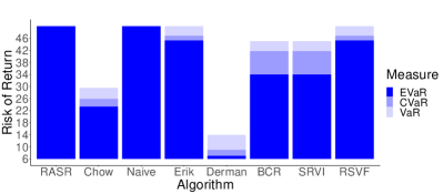
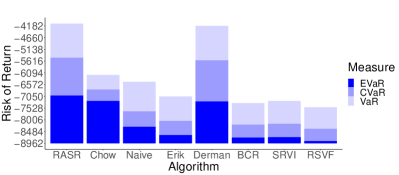
Figure 1: $\psi^{0.99}[\mathfrak{R}^{\pi}_{\infty}]$ in river-swim (left) and population (right) problems .

Table 1 summarizes the risk $\operatorname{EVaR}^{0.99}[\mathfrak{R}^{\pi}_{\infty}]$ for policies $\pi$ computed by RASR-EVaR and the baseline algorithms described above; please see Figure 1 and Section F for an evaluation with other risk measures. The results show that RASR-EVaR chooses the appropriate level of risk-aversion across all domains. The plots in Figure 1 help to visualize the situation for two of the domains. Derman is risk neutral and performs particularly poorly in river-swim, which has small but impactful epistemic risk. Risk averse algorithms, like RSVF and Erik, perform well in this domain. In contrast, Derman performs well in population, which involves large but inconsequential epistemic uncertainty. The risk-averse algorithms (RSVF, Erik, BCR) put too much emphasis on the epistemic uncertainty in this domain and compute policies that are too conservative.

Examining the results in Figure 1 closer leads one to several other important conclusions. First, the figures show that RASR-EVaR outperforms other algorithms even when the risk is evaluated using CVaR or VaR and may be a viable approximate approach optimizing these other risk measures. Second, the results in Figure 1 point to the importance of using the time dependent risk in the dynamic program equations. The Naive algorithm performs poorly in the population domain.

6 Related Work

Our RASR framework falls under the broader umbrella of robust and soft-robust MDP and RL. Robust optimization is a methodology that reduces the sensitivity of the solution to model errors Ben-Tal et al. (2009) and has been extensively studied in MDP Nilim and Ghaoui (2005); Iyengar (2005); Wiesemann et al. (2013); Ho et al. (2021) and RL Xu and Mannor (2012); Petrik and Subramanian (2014); Russel and Petrik (2019); Grand-Clement and Kroer (2021). Since robust MDPs often compute policies that are overly conservative, soft-robust (also known as Bayesian robust, light robust, or multi-model objectives) formulations were proposed as an alternative that can better balance robustness and the quality of an average solution (e.g., Ben-Tal et al. (2010); Derman et al. (2018); Mankowitz et al. (2019); Buchholz and Scheftelowitsch (2020)). Soft-robust algorithms replace the worst-case objective of robust optimization with risk-aversion to some distribution over uncertain models. Table 2 summarizes representative soft-robust and risk-averse algorithms studied in the MDP/RL literature. We defer a more comprehensive overview of related work to Section G.

Risk-averse MDP methods account only for the aleatory uncertainty in the return and do not explicitly consider the error in the model. The risk-averse formulations that are most closely related to our work use ERM. This list includes the results in the average reward Borkar and Jain (2014); Borkar and Meyn (2002); Borkar (2002) and those in the undiscounted finite-horizon settings Fei et al. (2020); Nass et al. (2020); Dowson et al. (2021). Note that some of these papers address risk-aversion in stochastic programming and not in MDPs Dowson et al. (2021). To the best of our knowledge, none of the prior work has studied ERM in the discounted case. We believe this is because ERM is not positive-homogeneous, which complicates using it with a discount factor, as shown in Theorem 2. Moreover, we are unaware of any EVaR adaptation of these earlier ERM algorithms. Most other formulations for risk-averse RL are based on VaR and CVaR Borkar and Jain (2014); Chow and Ghavamzadeh (2014); Tamar et al. (2015); Chow et al. (2018), which are not dynamically consistent and are NP hard to optimize. To build a DP in these formulations, one must augment the state space and optimize over a continuously infinite variable Bauerle and Ott (2011); Chow and Ghavamzadeh (2014); Chow et al. (2015); Pflug and Pichler (2016), which significantly complicates the computation in comparison with the time-dependent value functions in RASR-ERM. Finally, existing application of EVaR to MDPs have been limited to the nested (or Markov) formulation, which embeds the risk measure directly into the Bellman operator Ahmadi et al. (2021a, b); Dixit et al. (2021). The nested EVaR risk measure differs from the ordinary EVaR and generally approximates if only very poorly Iancu et al. (2015).

7 Conclusion and Future Work

We proposed RASR, a framework that can mitigate the risk associated with both model uncertainty (epistemic) and random dynamics (aleatory) in MDPs. We studied RASR with two separate risk measures: ERM and EVaR. In RASR-ERM, we derived the first exact DP formulation for ERM in discounted MDPs. We also showed that there optimal value function and deterministic Markov policies exist and can be computed using value iteration. For RASR-EVaR, we show that the RASR-EVaR objective can be optimized by reducing it to multiple RASR-ERM problems. Our empirical results highlight the utility of our RASR algorithms.

Future directions include scaling our RASR algorithms beyond tabular MDPs and dynamic epistemic uncertainty. It is also essential to better understand the relation between RASR and regularized (robust) MDPs Derman et al. (2021); Neu et al. (2017); Geist et al. (2019).

A Proofs of Section 2

The following proposition states a simple, but important property of the expectation operator which plays a crucial role in formulating the dynamic programs. The property is known under several different names, including the tower property, the law of total expectation, and the law of iterated expectations.

Proposition 10 (Tower Property, e.g., Proposition 3.4 in Ross and Peköz (2007)).

Any two random variables $X_{1},X_{2}\in\mathbb{X}$ satisfy that

$$\mathbb{E}[X_{1}]\;=\;\mathbb{E}\left[\mathbb{E}[X_{1}\mid X_{2}]\right]\leavevmode\nobreak\ .$$

A convenient way to represent ERM is to use its certainty equivalent form. This form relates the risk measure to the popular expected utility framework for decision-making Ben-Tal and Teboulle (2007). In the expected utility framework, one prefers a lottery (or a random reward) $X_{1}\in\mathbb{X}$ over $X_{2}\in\mathbb{X}$ if and only if

$$\mathbb{E}[u(X_{1})]\geq\mathbb{E}[u(X_{2})]\leavevmode\nobreak\ ,$$

for some increasing utility function $u\colon\mathbb{R}\to\mathbb{R}$.

The expected utility $\mathbb{E}[u(X)]$ is difficult to interpret because its units are incompatible with $X$. A more interpretable characterization of the expected utility is to use the certainty equivalent $z\in\mathbb{R}$, which is defined as the certain quantity that achieves the same expected utility as $X$:

$$\mathbb{E}[u(z)]=\mathbb{E}[u(X)],\quad\text{and therefore},\quad z=u^{-1}(\mathbb{E}[u(X)])\leavevmode\nobreak\ .$$ (15)

Algebraic manipulation from (15) then shows that ERM for any $X\in\mathbb{X}$ can be represented as the certainty equivalent

$$\operatorname{ERM}^{\alpha}[X]\;=\;u^{-1}(\mathbb{E}[u(X)])\leavevmode\nobreak\ ,$$ (16)

for the utility function $u:\mathbb{R}\to\mathbb{R}$ (see definition 2.1 in Ben-Tal and Teboulle (2007)) defined as

$$u(x)=\alpha^{-1}-\alpha^{-1}\cdot\operatorname{exp}\left(-\alpha\cdot x\right)\leavevmode\nobreak\ .$$

Because the function $u$ is strictly increasing, its inverse $u^{-1}\colon\mathbb{R}\to\mathbb{R}$ exists and equals to

$$u^{-1}(z)=-\alpha^{-1}\cdot\log(1-\alpha\cdot z)\leavevmode\nobreak\ .$$

Proof of Theorem 1.

The property is trivially true when $\alpha=0$ from Proposition 10 since $\operatorname{ERM}^{0}=\mathbb{E}$. The property then follows by algebraic manipulation for $\alpha>0$ using the certainty equivalent representation in (16) as

$$\operatorname{ERM}^{\alpha}\big{[}\operatorname{ERM}^{\alpha}[X_{1}\mid X_{2}]\big{]} =\operatorname{ERM}^{\alpha}\left[u^{-1}\left(\mathbb{E}[u(X_{1})\mid X_{2}]\right)\right]$$

$$=u^{-1}\left(\mathbb{E}\left[u\left(u^{-1}\left(\mathbb{E}[u(X_{1})\mid X_{2}]\right)\right)\right]\right)$$

$$=u^{-1}(\mathbb{E}\left[\mathbb{E}[u(X_{1})\mid X_{2}]\right])$$

$$=u^{-1}(\mathbb{E}[u(X_{1})])$$  Proposition 10

$$=\operatorname{ERM}^{\alpha}[X_{1}]\leavevmode\nobreak\ .$$

∎

B Proofs of Section 3

Input: Horizon $T<\infty$, risk level $\alpha>0$, terminal value $v_{T}(s),\;\forall s\in\mathcal{S}$

Output: Optimal value $(v_{t}^{\star})_{t=0}^{T}$ and policy $(\pi_{t}^{\star})_{t=0}^{T-1}$

1 Initialize $v^{\star}_{T}(s)\leftarrow v^{\prime}(s),\;\forall s\in\mathcal{S}$ ;

2 for $t=T-1,\dots,0$ do

3       Update $v_{t}^{\star}$ using (11) and $\pi_{t}^{\star}$ using (12);

4      

5return $v^{\star},\pi^{\star}$ ;

Algorithm 3 VI for finite-horizon RASR-ERM

Proof of Theorem 2.

The property is trivially true for $c=0$ or $\alpha=0$ because $\operatorname{ERM}^{0}=\mathbb{E}$ and $\operatorname{ERM}^{\alpha}[0]=0$. Then, for $c>0$ and $\alpha>0$, the property follows by rearranging the terms as

$$\operatorname{ERM}^{\alpha\cdot c}[X] =-\frac{1}{\alpha c}\log\big{(}\mathbb{E}[e^{-\alpha\cdot c\cdot X}]\big{)}$$

$$c\cdot\operatorname{ERM}^{\alpha\cdot c}[X] =-\frac{1}{\alpha}\log\big{(}\mathbb{E}[e^{-\alpha\cdot c\cdot X}]\big{)} c$$ Multiply by

$$=\operatorname{ERM}^{\alpha}[c\cdot X].$$

∎

In order to prove the correctness of the dynamic program formulation for the ERM objective, we need to formalize the soft-robust uncertainty model more rigorously. For the purpose of this discussion, we assume some fixed state $\hat{s}\in\mathcal{S}$, action $\hat{a}\in\mathcal{A}$, and a time step $\hat{t}\in 0,\dots,T-1$. To streamline the notation, we drop the subscripts of $f$, $P$, and $\bar{p}$ for $\hat{s}$, $\hat{a}$, and $\hat{t}$ in the subsequent discussion.

Now we formalize the nested distribution function, in which the random model $P$ governs the transition function of the random next state. Define a probability space $(\Omega\times\mathcal{S},2^{\Omega\times\mathcal{S}},\hat{f})$, which combines the uncertainty over the model $\omega$ and the next state $s^{\prime}\in\mathcal{S}$ at time $\hat{t}$ when taking an action $\hat{a}$ in a state $\hat{s}$. Define a 2-step filtration $\mathcal{F}_{0}=2^{\Omega}$ and $\mathcal{F}_{1}=2^{\Omega\times\mathcal{S}}$. The first step represents the model $P$ and the second step represents the choice of state $S$.

The random variable $S\colon(s,\omega)\mapsto s$ is measurable in $\mathcal{F}_{1}$ and represents the state transition. For the probability function $\hat{f}$ to be consistent with model probabilities $f$ defined in Section 2, the function $\hat{f}$ must satisfy that

$$f(\omega)=\sum_{s\in\mathcal{S}}\hat{f}(\omega,s),\quad\forall\omega\in\Omega\leavevmode\nobreak\ .$$ (17)

The vector-valued random variable $P\colon\Omega\to\Delta^{S}$ is measurable in $\mathcal{F}_{0}$ and represents the uncertain transition function. It is defined as

$$P(\omega,s)=P_{\hat{t}}(\cdot\mid\hat{s},\hat{a})\leavevmode\nobreak\ ,$$

for each $s\in\mathcal{S}$ and $\omega\in\Omega$. The random variable is independent of the component $s$ in the probability space. Finally, since $P$ governs the distribution of $S$, the function $\hat{f}$ must also satisfy that

$$\hat{f}(\omega,s^{\prime})=f(\omega)\cdot P(\omega)_{s^{\prime}},\quad\forall\omega\in\Omega,s^{\prime}\in\mathcal{S}\leavevmode\nobreak\ .$$ (18)

That this, this equality ensures that $S\sim P$.

Our goal now is to replace any random variable $X\colon\Omega\times\mathcal{S}\to\mathbb{R}$ defined on the entire filtration by a simpler random variable $\tilde{X}\colon\mathcal{S}\to\mathbb{R}$ measurable that has the same ERM value. The random variable $\tilde{X}$ is defined on a probability space $(\mathcal{S},2^{\mathcal{S}},\bar{p})$ with

$$\bar{p}(s)=\sum_{\omega\in\Omega}\hat{f}(\omega,s)=\sum_{\omega\in\Omega}f(\omega)\cdot P(\omega)_{s},\quad\forall s\in\mathcal{S}\leavevmode\nobreak\ .$$ (19)

Intuitively, the value $\bar{p}$ represents the mean transition probability of the uncertain $P$. The second equality in (19) follows immediately from (18). The following lemma shows that the ERM values of $X$ and $\tilde{X}$ coincide.

Lemma 11.

Suppose that random variables $P$, $X$, and $\tilde{X}$ are defined as above and that $X$ is independent of $\omega$:

$$X(\omega_{1},s)=X(\omega_{2},s),\quad\forall s\in\mathcal{S},\forall\omega_{1},\omega_{2}\in\Omega\leavevmode\nobreak\ .$$

Then, for any $\alpha\geq 0$, the entropic risk measure satisfies that

$$\operatorname{ERM}^{\alpha}[X]=\operatorname{ERM}^{\alpha}[\tilde{X}]=\operatorname{ERM}^{\alpha}[X\mid P=\bar{p}]\leavevmode\nobreak\ .$$ (20)

Proof.

We prove the property using the certainty equivalent representation of ERM in (16). For the utility function $u$ in (16), we get that

$$\mathbb{E}[u(x)] =\sum_{s\in\mathcal{S}}\sum_{\omega\in\Omega}u(X(s,\omega))\hat{f}(s,\omega)=\sum_{s\in\mathcal{S}}u(X(s))\left(\sum_{\omega\in\Omega}\hat{f}(s,\omega)\right)$$ (21)

$$\stackrel{{\scriptstyle\text{Eq.\leavevmode\nobreak\ \eqref{eq:P-definition-simple}}}}{{=}}\sum_{s\in\mathcal{S}}u(X(s))\left(\sum_{\omega\in\Omega}P(\omega)_{s}\cdot f(\omega)\right)$$

$$\stackrel{{\scriptstyle\text{Eq.\leavevmode\nobreak\ \eqref{eq:pbar-definition}}}}{{=}}\sum_{s\in\mathcal{S}}u(X(s))\left(\sum_{\omega\in\Omega}\bar{p}(\omega)_{s}\right)=\mathbb{E}[u(\tilde{X})]\leavevmode\nobreak\ .$$

Because $X$ is independent of $\omega$, the derivation above abbreviates it as $X(s)=X(\omega,s)$ for an arbitrary $\omega\in\Omega$. Equality (20) then follows from (16) and (21) as

$$\operatorname{ERM}^{\alpha}[X]=u^{-1}\left(\mathbb{E}[u(X)]\right)=u^{-1}\left(\mathbb{E}[u(\tilde{X})]\right)=\operatorname{ERM}^{\alpha}[\tilde{X}]\leavevmode\nobreak\ .$$

∎

Although Lemma 11 is stated for ERM, one could generalize it to CVaR and certain other risk measures that admit an optimized certainty equivalent representation Ben-Tal and Teboulle (2007).

Proof of Theorem 3.

The proof is divided into two steps, proving it for $v^{\pi}$ first and for $v^{\star}$ second.

We prove the result for $v^{\pi}$ for any fixed $\pi\in\Pi_{MR}$ by backward induction on $t$ from $t=T$ to $t=0$. In particular, we show that any $v^{\pi}_{t}$ that satisfies (10) must equal to its definition in (9) and is, therefore, also unique. The base case of the induction with $t=T$ is trivial because $v_{T}(s)=0$ for each $s\in\mathcal{S}$ by definition.

To prove the inductive step, we assume that any $v^{\pi}$ that satisfies the Bellman optimality condition in (10) must equal to (9) for $t+1\leq T$. We then prove that (10) implies (9) also for $t$ and each $s_{t}\in\mathcal{S}$.

Next, we first express the equality in (10) in terms of a random model $P_{t}$ and introduce random variables $A_{t}\colon\mathcal{A}\times\Omega\times\mathcal{S}\to\mathcal{A}$ and $S^{\prime\prime}\colon\mathcal{A}\times\Omega\times\mathcal{S}\to\mathcal{S}$ where $A_{t}(a,\omega,s)=a$ represents the actions taken and $S^{\prime\prime}(a,\omega,s)=s$ represents the next state for each $a\in\mathcal{A}$, $\omega\in\Omega$, $s\in\mathcal{S}$, and the randomized action is distributed as $A_{t}\sim\pi_{t}(s_{t})$. The random variables $A_{t}$ and $S^{\prime\prime}$ are defined over the joint probability space of $\mathcal{A}\times\Omega\times\mathcal{S}$ with a probability mass function

$$\hat{f}(a,\omega,s)=\pi_{t}(a\mid s_{t})\cdot f_{t}(\omega)\cdot P_{t}(\omega)(s\mid s_{t},a)\leavevmode\nobreak\ .$$

The function $\hat{f}$ is the joint probability over $a$, $\omega$, and $s$. Recall also that $S^{\prime}\sim\bar{p}_{t}(\cdot|s,A)$. The Bellman equation in (10) can be reformulated as

$$v_{t}^{\pi}(s_{t}) =\operatorname{ERM}^{\alpha\cdot\gamma^{t}}\left[r(s_{t},A_{t})+\gamma\cdot v_{t+1}^{\pi}(S^{\prime})\right]$$

$$=\operatorname{ERM}^{\alpha\cdot\gamma^{t}}\left[\operatorname{ERM}^{\alpha\cdot\gamma^{t}}\left[r(s_{t},A_{t})+\gamma\cdot v_{t+1}^{\pi}(S^{\prime})\mid A_{t}\right]\right]$$

$$=\operatorname{ERM}^{\alpha\cdot\gamma^{t}}\left[\operatorname{ERM}^{\alpha\cdot\gamma^{t}}\left[r(s_{t},A_{t})+\gamma\cdot v_{t+1}^{\pi}(S^{\prime\prime})\mid A_{t}\right]\right]$$

$$=\operatorname{ERM}^{\alpha\cdot\gamma^{t}}\left[r(s_{t},A_{t})+\gamma\cdot v_{t+1}^{\pi}(S^{\prime\prime})\right]\leavevmode\nobreak\ .$$ (22)

Above, Lemma 11 is applied to random variables $\tilde{X}=\operatorname{ERM}^{\alpha\cdot\gamma^{t}}\left[r(s_{t},A_{t})+\gamma\cdot v_{t+1}^{\pi}(S^{\prime})\mid A_{t}\right]$ and $X=\operatorname{ERM}^{\alpha\cdot\gamma^{t}}\left[r(s_{t},A_{t})+\gamma\cdot v_{t+1}^{\pi}(S^{\prime\prime})\mid A_{t}\right]$.

Next, by the induction hypothesis we can substitute the definition of $v_{t+1}^{\pi}(S^{\prime\prime})$ from (9) into (22) and use the positive quasi-homogeneity of ERM (Theorem 2) to get that

$$v_{t}^{\pi}(s_{t}) =\operatorname{ERM}^{\alpha\cdot\gamma^{t}}\left[r(s_{t},A_{t})+\gamma\cdot\operatorname{ERM}^{\alpha\cdot\gamma^{t+1}}\left[\sum_{t^{\prime}=t+1}^{T-1}\gamma^{t^{\prime}-t-1}\cdot r(S_{t^{\prime}},A_{t^{\prime}})\mid S_{t+1}=S^{\prime\prime}\right]\right]$$

$$=\operatorname{ERM}^{\alpha\cdot\gamma^{t}}\left[r(s_{t},A_{t})+\operatorname{ERM}^{\alpha\cdot\gamma^{t}}\left[\sum_{t^{\prime}=t+1}^{T-1}\gamma^{t^{\prime}-t}\cdot r(S_{t^{\prime}},A_{t^{\prime}})\mid S_{t+1}=S^{\prime\prime}\right]\right]\leavevmode\nobreak\ .$$

Here, $S_{t}=s_{t}$, $A_{t^{\prime}}\sim\pi_{t^{\prime}}(S_{t^{\prime}})$ for each $t^{\prime}\geq t+1$. The random variables $S_{t^{\prime}},t^{\prime}=t+1,\dots,T$ follow the policy $\pi$ and state transition probabilities.

Finally, using translation equivariance (A2 in Definition 19) and tower (Theorem 1) properties of ERM, we conclude that

$$v_{t}^{\pi}(s_{t}) =\operatorname{ERM}^{\alpha\cdot\gamma^{t}}\left[r(S_{t},A_{t})+\operatorname{ERM}^{\alpha\cdot\gamma^{t}}\left[\sum_{t^{\prime}=t+1}^{T-1}\gamma^{t^{\prime}-t}\cdot r(S_{t^{\prime}},A_{t^{\prime}})\mid S_{t+1}=S^{\prime\prime},A_{t}\right]\mid S_{t}=s_{t}\right]$$

$$=\operatorname{ERM}^{\alpha\cdot\gamma^{t}}\left[\operatorname{ERM}^{\alpha\cdot\gamma^{t}}\left[r(S_{t},A_{t})+\sum_{t^{\prime}=t+1}^{T-1}\gamma^{t^{\prime}-t}\cdot r(S_{t^{\prime}},A_{t^{\prime}})\mid S_{t+1}=S^{\prime\prime},A_{t}\right]\mid S_{t}=s_{t}\right]$$

$$=\operatorname{ERM}^{\alpha\cdot\gamma^{t}}\left[\operatorname{ERM}^{\alpha\cdot\gamma^{t}}\left[\sum_{t^{\prime}=t}^{T-1}\gamma^{t^{\prime}-t}\cdot r(S_{t^{\prime}},A_{t^{\prime}})\mid S_{t+1}=S^{\prime\prime},A_{t}\right]\mid S_{t}=s_{t}\right]$$

$$=\operatorname{ERM}^{\alpha\cdot\gamma^{t}}\left[\sum_{t^{\prime}=t}^{T-1}\gamma^{t^{\prime}-t}\cdot r(S_{t^{\prime}},A_{t^{\prime}})\mid S_{t}=s_{t}\right]\leavevmode\nobreak\ .$$

The derivation above shows that any $v^{\pi}$ that satisfies the Bellman equation in (10) is unique and satisfies the definition in (9).

To prove the second part of the theorem, which concerns $v^{\star}$, we formally define the optimal value function $v^{\star}$ for each $t=0,\dots,T$ as

$$v^{\star}_{t}(s)\;=\;\max_{\pi\in\Pi_{MR}^{t}}\operatorname{ERM}^{\alpha\cdot\gamma^{t}}\left[\sum_{t^{\prime}=t}^{T-1}\gamma^{t^{\prime}-t}\cdot R^{\pi}_{t^{\prime}}\mid S_{t}=s\right],\quad\forall s\in\mathcal{S}\leavevmode\nobreak\ .$$ (23)

Here, the set $\Pi_{MR}^{t}$ represents the randomized Markov policies for time steps $t,\dots,T-1$.

The proof for the optimal value function $v^{\star}$ now proceeds by backward induction analogously to the proof of (10) with the difference that it incorporates the optimization over actions. As before, the base case with $t=T$ is trivial because $v^{\star}_{T}(s)=0$ for each $s\in\mathcal{S}$.

To prove the inductive step, assume that (11) implies (23) for $t+1\leq T$ and show the implication for $t$ and each $s_{t}\in\mathcal{S}$. Let $S^{\prime\prime}$ and $A_{t}$ be defined as in the first part of the proof, except that $A_{t}$ need not be distributed according to $\pi_{t}$. Then from Lemma 11, we formulate the Bellman equation in terms of $S^{\prime\prime}$ that is jointly random over $\Omega$ and $\mathcal{S}$ as

$$v_{t}^{\star}(s_{t}) =\max_{a\in\mathcal{A}}\operatorname{ERM}^{\alpha\cdot\gamma^{t}}\left[r(s_{t},A_{t})+\gamma\cdot v_{t+1}^{\star}(S^{\prime})\mid A_{t}=a\right]$$

$$=\max_{a\in\mathcal{A}}\operatorname{ERM}^{\alpha\cdot\gamma^{t}}\left[r(s_{t},A_{t})+\gamma\cdot v_{t+1}^{\star}(S^{\prime\prime})\mid A_{t}=a\right]\leavevmode\nobreak\ .$$

Then, Lemma 15 shows that the maximization over actions can be replaced by a maximization over randomized policies which consider distributions over actions as

$$v^{\star}(s_{t}) =\max_{a\in\mathcal{A}}\operatorname{ERM}^{\alpha\cdot\gamma^{t}}\left[r(s_{t},A_{t})+\gamma\cdot v_{t+1}^{\star}(S^{\prime\prime})\mid A_{t}=a\right]$$

$$=\max_{d\in\Delta^{A}}\operatorname{ERM}^{\alpha\cdot\gamma^{t}}\left[r(s_{t},A_{t})+\gamma\cdot v_{t+1}^{\star}(S^{\prime\prime})\mid A_{t}\sim d\right]\leavevmode\nobreak\ .$$ (24)

Next, we can substitute the definition of $v_{t+1}^{\star}(S^{\prime\prime})$ from (23) into (24) by the induction hypothesis and use the positive quasi-homogeneity of ERM (Theorem 2) to get that

$$v_{t}^{\star}(s_{t}) =\max_{d\in\Delta^{A}}\operatorname{ERM}^{\alpha\cdot\gamma^{t}}\left[r(S_{t},A_{t})+\gamma\max_{\pi\in\Pi_{MR}^{t+1}}\operatorname{ERM}^{\alpha\cdot\gamma^{t+1}}\left[\sum_{t^{\prime}=t+1}^{T-1}\gamma^{t^{\prime}-t-1}r(S_{t^{\prime}},A_{t^{\prime}})\mid S_{t+1}=S^{\prime\prime}\right]\right]$$

$$=\max_{d\in\Delta^{A}}\operatorname{ERM}^{\alpha\cdot\gamma^{t}}\left[r(S_{t},A_{t})+\max_{\pi\in\Pi_{MR}^{t+1}}\operatorname{ERM}^{\alpha\cdot\gamma^{t}}\left[\sum_{t^{\prime}=t+1}^{T-1}\gamma^{t^{\prime}-t}\cdot r(S_{t^{\prime}},A_{t^{\prime}})\mid S_{t+1}=S^{\prime\prime}\right]\right]\leavevmode\nobreak\ .$$

Here, $S_{t}=s_{t}$, $A_{t}\sim d$, and $A_{t^{\prime}}\sim\pi_{t^{\prime}}(S_{t^{\prime}})$ for each $t^{\prime}\geq t+1$ and the random variables $S_{t^{\prime}},t^{\prime}=t+1,\dots,T$ are governed by $\pi_{t^{\prime}}$ and transition probabilities. We can move $\gamma$ inside the maximization operator because it is non-negative.

Finally, using monotonicity (A1 in Definition 19), translation equivariance (A2 in Definition 19) and tower (Theorem 1) properties of ERM, we conclude that

$$v_{t}^{\star}(s_{t}) =\max_{d\in\Delta^{A}}\operatorname{ERM}^{\alpha\cdot\gamma^{t}}\left[r(S_{t},A_{t})+\max_{\pi\in\Pi_{MR}^{t+1}}\operatorname{ERM}^{\alpha\cdot\gamma^{t}}\left[\sum_{t^{\prime}=t+1}^{T-1}\gamma^{t^{\prime}-t}\cdot r(S_{t^{\prime}},A_{t^{\prime}})\mid S_{t+1}=S^{\prime\prime},A_{t}\right]\right]$$

$$=\max_{d\in\Delta^{A}}\operatorname{ERM}^{\alpha\cdot\gamma^{t}}\left[\max_{\pi\in\Pi_{MR}^{t+1}}\operatorname{ERM}^{\alpha\cdot\gamma^{t}}\left[r(S_{t},A_{t})+\sum_{t^{\prime}=t+1}^{T-1}\gamma^{t^{\prime}-t}\cdot r(S_{t^{\prime}},A_{t^{\prime}})\mid S_{t+1}=S^{\prime\prime},A_{t}\right]\right]$$

$$=\max_{d\in\Delta^{A}}\operatorname{ERM}^{\alpha\cdot\gamma^{t}}\left[\max_{\pi\in\Pi_{MR}^{t+1}}\operatorname{ERM}^{\alpha\cdot\gamma^{t}}\left[\sum_{t^{\prime}=t}^{T-1}\gamma^{t^{\prime}-t}\cdot r(S_{t^{\prime}},A_{t^{\prime}})\mid S_{t+1}=S^{\prime\prime},A_{t}\right]\right]$$

$$=\max_{\pi\in\Pi_{MR}^{t}}\operatorname{ERM}^{\alpha\cdot\gamma^{t}}\left[\sum_{t^{\prime}=t}^{T-1}\gamma^{t^{\prime}-t}\cdot r(S_{t^{\prime}},A_{t^{\prime}})\mid S_{t}=s_{t}\right]\leavevmode\nobreak\ .$$

As before, $S_{t}=s_{t}$, $A_{t}\sim d$, and $A_{t^{\prime}}\sim\pi_{t^{\prime}}(S_{t^{\prime}})$ for each $t^{\prime}\geq t+1$.The derivation above shows that any $v^{\star}$ that satisfies (11) equals to the definition in (23) and is, therefore, unique. ∎

Proof of Corollary 4.

The proof follows immediately by reformulating the objective in (13) as the dynamic programming equations in Theorem 3. These dynamic programming equations are identical for the dynamic programming equations for a risk-averse ERM objective with the average model $\bar{p}=(\bar{p}_{t})_{t=0}^{T-1}$ as defined in Theorem 3. ∎

Proof of Theorem 5.

Following the notation of Chapter 4 in Puterman (2005), let $\mathcal{H}_{t}$ be the set of all histories up to time $t$ inclusively. Let the optimal history-dependent value function be $u_{t}^{\star}\colon\mathcal{H}_{t}\to\mathbb{R},t=0,\dots,T$. The value function $u^{\star}=(u^{\star}_{t})_{t=0}^{T}$ is achieved by the optimal history-dependent policy because the state and actions are finite and, therefore, the space of randomized history-dependent policies is compact.

The proof proceeds in 2 steps. First, we show that $v^{\star}$ attains the return of the optimal history-dependent value function:

$$u^{\star}_{t}(h_{t})=v^{\star}_{t}(s_{t})\quad\forall h_{t}\in\mathcal{H}_{t},t=0,\dots,T\leavevmode\nobreak\ ,$$

where $s_{t}$ is the $t$-th and final state in the history $h_{t}$. This result is a consequence of the dynamic programming formulation in Theorem 3.

An argument analogous to the proof of Theorem 4.4.2(a) in Puterman (2005) shows that $u^{\star}_{t}(h_{t})$ only depends on $s_{t}$, which is the final state in the history $h_{t}$.

Using the standard backward-induction argument on $t$, assume that $u^{\star}_{t+1}(h_{t+1})=v^{\star}_{t+1}(s_{t+1})$ holds and we prove that $u^{\star}_{t}(h_{t})=v^{\star}_{t}(s_{t})$. Let $d_{t}\in\Delta^{A}$ be the randomized decision-rule (action) that achieves $u^{\star}(h_{t})$ where $s_{t}$ is the last state in the history $h_{t}$. Then applying Theorem 3 applied to $u^{\star}$ (using history-dependent state space) and the inductive assumption we conclude that

$$u^{\star}_{t}(h_{t}) =\operatorname{ERM}^{\alpha\cdot\gamma^{t}}\left[r(s_{t},A)+\gamma\cdot u_{t+1}^{\star}((h_{t},A,S^{\prime}))\mid A\sim d_{t}\right]$$

$$=\operatorname{ERM}^{\alpha\cdot\gamma^{t}}\left[r(s_{t},A)+\gamma\cdot v_{t+1}^{\star}(S^{\prime})\mid A\sim d_{t}\right]$$

$$=\max_{d\in\Delta^{A}}\operatorname{ERM}^{\alpha\cdot\gamma^{t}}\left[r(s_{t},A)+\gamma\cdot v_{t+1}^{\star}(S^{\prime})\mid A\sim d\right]\leavevmode\nobreak\ .$$

The notation $(h_{t},A,S^{\prime})$ signifies a new history $h_{t+1}$ constructed by appending the action $A$ and state $S^{\prime}$. The state $S^{\prime}$ is a random variable distributed according to $\bar{p}(\cdot\mid s_{t},A)$. Then, using Section D and the Bellman optimality condition in (11), we conclude that

$$u^{\star}_{t}(h_{t}) =\max_{d\in\Delta^{A}}\operatorname{ERM}^{\alpha\cdot\gamma^{t}}\left[r(s_{t},A)+\gamma\cdot v_{t+1}^{\star}(S^{\prime})\mid A\sim d\right]$$

$$=v^{\star}_{t}(s_{t}).$$

The second part of the proof is to show that $\pi^{\star}$ achieves the optimal value function $v^{\star}$:

$$v_{t}^{\pi^{\star}}(s)=v_{t}^{\star}(s),\quad\forall s\in\mathcal{S},t=0,\dots,T\leavevmode\nobreak\ .$$

This result follows using the standard backward induction argument and algebraic manipulation from Theorem 3. The derivation relies on the fact that $\mathcal{A}$ is finite and the maximum in (11) exists (and is achieved). The fact that $\pi^{\star}$ is greedy to $v^{\star}$ is trivial from the definition of a greedy policy. ∎

The following lemma plays an important role in bounding the difference between ERM and the expectation. This result serves to bound the error of replacing the risk-averse value function by a risk-neutral value function in Algorithm 1.

Lemma 12.

Let $X\in\mathbb{X}$ be a bounded random variable such that $x_{\min}\leq X\leq x_{\max}$ a.s. Then, for any risk level $\alpha>0$, we have $\mathbb{E}[X]-\epsilon(\alpha)\leq\operatorname{ERM}^{\alpha}[X]\leq\mathbb{E}[X]$, where

$$\epsilon(\alpha)\;=\;8^{-1}\cdot\alpha\cdot(x_{\max}-x_{\min})^{2}\,.$$

The gap vanishes with a decreasing risk: $\lim_{\alpha\to 0}\epsilon(\alpha)=0$.

Proof.

To streamline the notation, let $X=\mathfrak{R}^{\pi}_{T}$ for any policy $\pi$ which is bounded between $x_{\min}$ and $x_{\max}$. Also, recall that the Hoeffding’s lemma shows that for any $\forall\lambda\in\real$ Massart (2003); Boucheron et al. (2013)

$$\mathbb{E}[e^{\lambda X}]\leq e^{\lambda\mathbb{E}[x]+\frac{\lambda^{2}(x_{\max}-x_{\min})^{2}}{8}}\leavevmode\nobreak\ .$$

Applying $\log$ to both sides of the inequality above gives

$$\log\big{(}\mathbb{E}[e^{\lambda X}]\big{)}\leq\lambda\mathbb{E}[x]+\frac{\lambda^{2}(x_{\max}-x_{\min})^{2}}{8}\leavevmode\nobreak\ .$$

Then substitute $\lambda=-\alpha$ into the equation above to by algebraic manipulation that

$$\log\big{(}\mathbb{E}[e^{-\alpha X}]\big{)} \leq-\alpha\cdot\mathbb{E}[x]+\frac{\alpha^{2}\cdot(x_{\max}-x_{\min})^{2}}{8}$$

$$-\frac{1}{\alpha}\log\big{(}\mathbb{E}[e^{-\alpha X}]\big{)} \geq\mathbb{E}[x]-\frac{\alpha(x_{\max}-x_{\min})^{2}}{8}$$

$$\mathbb{E}[x]-\frac{\alpha(x_{\max}-x_{\min})^{2}}{8} \leq\operatorname{ERM}^{\alpha}[X]\leavevmode\nobreak\ .$$

Therefore, $\mathbb{E}[X]-\epsilon(\alpha)\leq\operatorname{ERM}^{\alpha}[X]$ where $\epsilon(\alpha)=8^{-1}\alpha(x_{\max}-x_{\min})^{2}$.

The second inequality $\operatorname{ERM}^{\alpha}[X]\leq\mathbb{E}[X]$ follows immediately from the dual representation of ERM used in the proof of Lemma 15. ∎

Proof of Theorem 6.

The main idea of the proof is to lower-bound the value function $v^{\hat{\pi}^{\star}}$ of the policy $\hat{\pi}^{\star}$ using the value function $v^{\infty}$ of the optimal risk-neutral policy. Recall that Lemma 12 bounds the error between the risk-neutral and ERM value function of any policy $\pi$ and any $t=0,\dots$ as

$$0\leq v^{\infty}_{\pi}-v^{\pi}_{t}\leq\frac{\alpha\cdot\gamma^{t}\cdot(\triangle r)^{2}}{8\cdot(1-\gamma)^{2}}\leavevmode\nobreak\ .$$ (25)

The symbol $v^{\infty}_{\pi}$ denotes the ordinary risk-neutral ($\operatorname{ERM}^{0}$) $\gamma$-discounted infinite-horizon value function of the policy $\pi$. Note that this value function is stationary. The left-hand side of the equation above holds because $\mathbb{E}$ is an upper bound on the ERM.

As the first step of the proof, we bound the error at time $T^{\prime}$ as follows. Consider any state $s\in\mathcal{S}$, then:

$$v^{\star}_{T^{\prime}}(s)-v_{T^{\prime}}^{\hat{\pi}^{\star}}(s) \leq v^{\star}_{T^{\prime}}(s)-v^{\infty}_{\hat{\pi}^{\star}}(s)+\frac{\alpha\cdot\gamma^{T^{\prime}}\cdot(\triangle r)^{2}}{8\cdot(1-\gamma)^{2}}$$ from r.h.s of (25)

$$\leq v^{\infty}_{\pi^{\star}}(s)-v^{\infty}_{\hat{\pi}^{\star}}(s)+\frac{\alpha\cdot\gamma^{T^{\prime}}\cdot(\triangle r)^{2}}{8\cdot(1-\gamma)^{2}}$$ from l.h.s. of (25)

$$\leq\frac{\alpha\cdot\gamma^{T^{\prime}}\cdot(\triangle r)^{2}}{8\cdot(1-\gamma)^{2}} \text{from }\hat{\pi}^{\star}\in\arg\max_{\pi\in\Pi}v^{\infty}_{\pi}(s)\leavevmode\nobreak\ .$$

As the second step of the proof, we construct an approximation $u_{t}\in\mathbb{R}^{S},t=0,\dots,T^{\prime}$ of the value function $v_{t}^{\hat{\pi}^{\star}}$ for $t=0,\dots,T^{\prime}-1$ and all $s\in\mathcal{S}$ as:

$$u_{T^{\prime}}(s) =v^{\infty}_{\hat{\pi}^{\star}}-\frac{\alpha\cdot\gamma^{T^{\prime}}\cdot(\triangle r)^{2}}{8\cdot(1-\gamma)^{2}}$$

$$u_{t}(s) =\max_{a\in\mathcal{A}}\operatorname{ERM}^{t\cdot\gamma^{t}}\left[r(s,a)+\gamma\cdot u_{t+1}(S^{\prime}_{t+1,a})\right]$$

$$=\operatorname{ERM}^{t\cdot\gamma^{t}}\left[r(s,\hat{\pi}^{\star}(s))+\gamma\cdot u_{t+1}(S^{\prime}_{t+1,\hat{\pi}^{\star}(s)})\right]\leavevmode\nobreak\ ,$$

where $S^{\prime}_{t+1,a}$ denotes the random variable that represents the state that follows $s$ at time $t+1$ after taking an action $a$. The last equality holds from the definition of $\hat{\pi}^{\star}_{t}$ being greedy to $u_{t}$; subtracting a constant from all states does not change the greedy policy. The function $u_{t}$ is constructed to be a lower bound on $v_{t}^{\hat{\pi}^{\star}}$ and at the same time be a value such that $\hat{\pi}^{\star}$ is greedy to it.

From (25), we have that $v^{\pi}_{T^{\prime}}(s)\geq u_{T^{\prime}}(s)$ for all $s\in\mathcal{S}$. Then, assuming $v^{\pi}_{t+1}(s)\geq u_{t+1}(s)$ for all $s\in\mathcal{S}$, we can use backward induction on $t$ to show that

$$v^{\hat{\pi}^{\star}}_{t}(s)-u_{t}(s) =\operatorname{ERM}^{t\cdot\gamma^{t}}\left[r(s,\hat{\pi}^{\star}_{t}(s))+\gamma\cdot v^{\hat{\pi}^{\star}}_{t+1}(S^{\prime}_{t+1,\hat{\pi}^{\star}_{t}(s)})\right]-$$

$$\qquad-\operatorname{ERM}^{t\cdot\gamma^{t}}\left[r(s,\hat{\pi}^{\star}_{t}(s))+\gamma\cdot u_{t+1}(S^{\prime}_{t+1,\hat{\pi}^{\star}_{t}(s)})\right]$$

$$\stackrel{{\scriptstyle\text{(a)}}}{{=}}\operatorname{ERM}^{t\cdot\gamma^{t}}\left[\gamma\cdot v^{\hat{\pi}^{\star}}_{t+1}(S^{\prime}_{t+1,\hat{\pi}^{\star}_{t}(s)})\right]-\operatorname{ERM}^{t\cdot\gamma^{t}}\left[\gamma\cdot u_{t+1}(S^{\prime}_{t+1,\hat{\pi}^{\star}_{t}(s)})\right]$$

$$\stackrel{{\scriptstyle\text{(b)}}}{{=}}\gamma\cdot\left(\operatorname{ERM}^{t\cdot\gamma^{t+1}}\left[v^{\hat{\pi}^{\star}}_{t+1}(S^{\prime}_{t+1,\hat{\pi}^{\star}_{t}(s)})\right]-\operatorname{ERM}^{t\cdot\gamma^{t+1}}\left[u_{t+1}(S^{\prime}_{t+1,\hat{\pi}^{\star}_{t}(s)})\right]\right)$$

$$\stackrel{{\scriptstyle\text{(c)}}}{{\geq}}0\leavevmode\nobreak\ .$$

The equality (a) is shown by subtracting the constant reward from both terms which can be done because ERM is translation equivariant. The equality (b) follows from the positive quasi-homogeneity in Theorem 2, and (c) follows from the monotonicity of ERM.

As the third step of the proof, we show for each $s\in\mathcal{S}$ and $t=0,\dots,T^{\prime}$ that

$$v_{t}^{\star}(s)-u_{t}(s)\leq\gamma^{T^{\prime}-t}\cdot\frac{\alpha\cdot\gamma^{T^{\prime}}\cdot(\triangle r)^{2}}{8\cdot(1-\gamma)^{2}}\leavevmode\nobreak\ .$$ (26)

The inequality (26) holds for $t=T^{\prime}$ from (25) and the construction of $u_{T^{\prime}}$. To prove (26) by induction, assume it holds for $t+1$. Then for each $s\in\mathcal{S}$:

$$v_{t}^{\star}(s)-u_{t}(s) \stackrel{{\scriptstyle\text{(a)}}}{{=}}\operatorname{ERM}^{t\cdot\gamma^{t}}\left[r(s,\pi^{\star}_{t}(s))+\gamma\cdot v^{\star}_{t+1}(S^{\prime}_{t+1,\pi^{\star}_{t}(s)})\right]-$$

$$\qquad-\operatorname{ERM}^{t\cdot\gamma^{t}}\left[r(s,\hat{\pi}^{\star}_{t}(s))+\gamma\cdot u_{t+1}(S^{\prime}_{t+1,\hat{\pi}^{\star}_{t}(s)})\right]$$

$$\stackrel{{\scriptstyle\text{(b)}}}{{=}}\operatorname{ERM}^{t\cdot\gamma^{t}}\left[r(s,\pi^{\star}_{t}(s))+\gamma\cdot v^{\star}_{t+1}(S^{\prime}_{t+1,\pi^{\star}_{t}(s)})\right]-$$

$$\qquad-\operatorname{ERM}^{t\cdot\gamma^{t}}\left[r(s,\pi^{\star}_{t}(s))+\gamma\cdot u_{t+1}(S^{\prime}_{t+1,\pi^{\star}_{t}(s)})\right]$$

$$\stackrel{{\scriptstyle\text{(c)}}}{{=}}\operatorname{ERM}^{t\cdot\gamma^{t}}\left[\gamma\cdot v^{\hat{\pi}^{\star}}_{t+1}(S^{\prime}_{t+1,\pi^{\star}_{t}(s)})\right]-\operatorname{ERM}^{t\cdot\gamma^{t}}\left[\gamma\cdot u_{t+1}(S^{\prime}_{t+1,\pi^{\star}_{t}(s)})\right]$$

$$\stackrel{{\scriptstyle\text{(d)}}}{{=}}\gamma\cdot\left(\operatorname{ERM}^{t\cdot\gamma^{t+1}}\left[v^{\pi^{\star}}_{t+1}(S^{\prime}_{t+1,\pi^{\star}(s)})\right]-\operatorname{ERM}^{t\cdot\gamma^{t+1}}\left[u_{t+1}(S^{\prime}_{t+1,\pi^{\star}(s)})\right]\right)$$ (27)

The identity (a) is true by the definition of $v^{\star}_{t}$ and $u_{t}$, (b) follows from $\hat{\pi}^{\star}$ being greedy to $u$, (c) follows by subtracting the constant reward from both terms which can be done because ERM is translation equivariant. Finally, the equality (d) follows from the positive quasi-homogeneity in Theorem 2. Then, from the inductive assumption we get the desired inequality from the monotonicity and translation equivariance of ERM by bounding the terms in (27) above as:

$$v_{t+1}^{\pi^{\star}}(s)-u_{t+1}(s) \leq\gamma^{T^{\prime}-t-1}\cdot\frac{\alpha\cdot\gamma^{T^{\prime}}\cdot(\triangle r)^{2}}{8\cdot(1-\gamma)^{2}}\qquad\forall s\in\mathcal{S}$$

$$\operatorname{ERM}^{t\cdot\gamma^{t+1}}[v_{t+1}^{\pi^{\star}}(S)]-\operatorname{ERM}^{t\cdot\gamma^{t+1}}[u_{t+1}(S)] \leq\gamma^{T^{\prime}-t-1}\cdot\frac{\alpha\cdot\gamma^{T^{\prime}}\cdot(\triangle r)^{2}}{8\cdot(1-\gamma)^{2}}$$ (28)

$$\gamma\cdot(\operatorname{ERM}^{t\cdot\gamma^{t+1}}[v_{t+1}^{\pi^{\star}}(S)]-\operatorname{ERM}^{t\cdot\gamma^{t+1}}[u_{t+1}(S)]) \leq\gamma^{T^{\prime}-t}\cdot\frac{\alpha\cdot\gamma^{T^{\prime}}\cdot(\triangle r)^{2}}{8\cdot(1-\gamma)^{2}}\leavevmode\nobreak\ .$$

Because inequality in (28) holds for any random variables $S$, we can substitute $S=S^{\prime}_{t+1,\pi^{\star}_{t+1}(s)}$ from (27). The substitution then proves the bound on $u_{t}$.

The theorem then follows from the properties established above as

$$\operatorname{ERM}^{\alpha}\big{[}\mathfrak{R}_{\infty}^{\pi^{\star}}\mid P=\bar{p}\big{]}-\operatorname{ERM}^{\alpha}\big{[}\mathfrak{R}_{\infty}^{\hat{\pi}^{\star}}\mid P=\bar{p}\big{]} =v_{0}^{\star}(s_{0})-v^{\hat{\pi}^{\star}}_{0}(s_{0})\leq v_{0}^{\star}(s_{0})-u_{0}$$

$$\leq\frac{\alpha\cdot\gamma^{2\cdot T^{\prime}}\cdot(\triangle r)^{2}}{8\cdot(1-\gamma)^{2}}\leavevmode\nobreak\ .$$

∎

C Proofs of Section 4

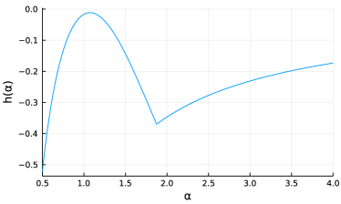
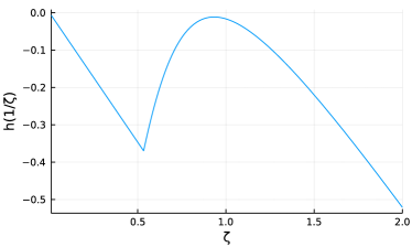
Figure 2: Plots of $h(\alpha)$ (left) and $h(\zeta^{-1})$ (right) for $\beta=0.5$, which are used in the proof of Proposition 13.

Recall that the function $h\colon\mathbb{R}\to\mathbb{R}$ is defined in (14) as

$$h(\alpha)\;=\;\max_{\pi\in\Pi_{MR}}\,\left(\operatorname{ERM}^{\alpha}[\mathfrak{R}_{T}^{\pi}]+\alpha^{-1}\cdot\log(1-\beta)\right)\leavevmode\nobreak\ .$$

Because solving RASR-EVaR reduces to computing $\max_{\alpha\geq 0}h(\alpha)$, it would be ideal if it were concave or at least quasi-concave. When $|\Pi_{MR}|=1$, it is known that the function $\zeta\mapsto h(\zeta^{-1})$ is concave Ahmadi-Javid (2012) and $h$ is quasi-concave. Unfortunately, the following proposition shows that $h$ is not necessarily quasi-concave when $|\Pi_{MR}|>1$ which precludes the use of more efficient optimization methods when solving $\max_{\alpha\geq 0}h(\alpha)$.

Proposition 13.

There exists an MDP and $\beta\in[0,1)$ such that the function $h\colon\mathbb{R}\to\mathbb{R}$ defined in (14) is neither concave nor convex either in $\alpha$ or $\alpha^{-1}$.

Proof.

We show the property by constructing a counter-example for which the function $h$ is not concave. Consider a risk-averse problem (no epistemic uncertainty) with an MDP with states $\mathcal{S}=\{s_{0},s_{1},s_{2},s_{3}\}$, actions $\mathcal{A}=\{a_{1},a_{2}\}$, and a finite-horizon objective with $\gamma=1$ and $T=2$. The initial state is $s_{0}$. Define the MDP’s parameters as

$$p(\cdot\mid s_{0},a_{1}) =[0,0,1,0]$$

$$p(\cdot\mid s_{0},a_{2}) =[0,0.02,0,0.98]$$

$$r(\cdot,a_{i}) =[-2,0,1],\quad i\in\{1,2\}\leavevmode\nobreak\ .$$

The transition probabilities from $s_{1},s_{2},s_{3}$ are irrelevant because of the limited horizon $T=2$. Setting $\beta=0.5$, one can easily verify that $h(\alpha)$ and $h(\zeta^{-1})$ are not quasi-concave by computing $h(1)$, $h(2)$, and $h(4)$. Figure 2 shows the plots of both $h(\alpha)$ and $h(\zeta^{-1})$. ∎

Proof of Theorem 7.

We prove the contra-positive: If $\pi^{\star}$ is not optimal policy in RASR-ERM for all $\alpha>0$, then $\pi^{\star}$ is not an optimal solution to RASR-EVaR. Assume $\pi^{\star}$ is not an optimal policy for all $\alpha>0$, and $\pi_{\alpha}$ is an optimal policy for RASR-ERM^α,

$$\operatorname{ERM}^{\alpha}\left[X^{\pi^{\star}}\right] <\operatorname{ERM}^{\alpha}\left[X^{\pi_{\alpha}}\right]\qquad,\forall\leavevmode\nobreak\ \alpha>0$$

$$\sup_{\alpha>0}\left\{\operatorname{ERM}^{\alpha}[X^{\pi^{\star}}]+\frac{\log(1-\beta)}{\alpha}\right\} <\sup_{\alpha>0}\left\{\operatorname{ERM}^{\alpha}[X^{\pi_{\alpha}}]+\frac{\log(1-\beta)}{\alpha}\right\}$$

$$\operatorname{EVaR}^{\beta}[X] <\sup_{\alpha>0}\left\{\operatorname{ERM}^{\alpha}\left[X^{\pi_{\alpha}}\right]+\frac{\log(1-\beta)}{\alpha}\right\}$$

We prove that if $\pi^{\star}$ is not optimal policy in RASR-ERM for all $\alpha>0$, then $\pi^{\star}$ is not an optimal solution to RASR-EVaR. With contra-positive we prove that if $\pi^{\star}$ is an optimal solution to RASR-EVaR^β in (13) then there exists a value $\alpha^{\star}$ such that $\pi^{\star}$ is optimal in RASR-ERM with risk level $\alpha=\alpha^{\star}$. ∎

Proof of Corollary 8.

Theorem 7 shows that the optimal policy $\pi^{\star}$ for $\operatorname{EVaR}^{\beta}[X^{\pi^{\star}}]$ implies there exists $\alpha^{\star}$ such that $\operatorname{ERM}^{\alpha^{\star}}[X^{\pi^{\star}}]$ is optimal in RASR-ERM and Theorem 5 shows that there exists a Markov deterministic time-dependent optimal policy $\pi^{\star}=(\pi_{t}^{\star})_{t=0}^{T-1}\in\Pi_{MD}$ for (8). Therefore there exists a Markov deterministic time-dependent optimal policy $\pi^{\star}$ which optimizes the EVaR objective in (13).

The second part of the corollary can be shown as follows. For any policy $\pi\in\Pi_{MR}$, the RASR-EVaR objective in (8) can be written as

$$\operatorname{EVaR}^{\beta}\left[\mathfrak{R}_{T}^{\pi}\right] =\sup_{\alpha>0}\left(\operatorname{ERM}^{\alpha}[\mathfrak{R}_{T}^{\pi}]+\frac{\log(1-\beta)}{\alpha}\right)$$

$$=\sup_{\alpha>0}\left(\operatorname{ERM}^{\alpha}[\mathfrak{R}_{T}^{\pi}\mid P=\bar{p}]+\frac{\log(1-\beta)}{\alpha}\right)$$

$$=\operatorname{EVaR}^{\beta}\left[\mathfrak{R}_{T}^{\pi}\mid P=\bar{p}\right]\;.$$

∎

The following lemma plays an important role in bounding the error introduced by discretizing the risk level $\alpha$ in Algorithm 2.

Lemma 14.

Suppose that $\alpha^{\star}$ attains the maximum in (14) then $\alpha_{0}\geq\alpha^{\star}\geq\alpha_{K}$, and $h(\hat{\alpha})\geq h(\alpha_{k})$ for $k=0,\dots,K$ and some $\alpha_{0}\geq\dots\geq\alpha_{K}$. Then

$$h(\alpha^{\star})-h(\hat{\alpha})\leq\log(1-\beta)\max_{k\in 0,\dots,K-1}\left(\alpha_{k}^{-1}-\alpha_{k+1}^{-1}\right)\leavevmode\nobreak\ .$$

Also, $h(\alpha^{\star})-h(\hat{\alpha})\leq-\log(1-\beta)\alpha_{0}^{-1}$ when $\alpha^{\star}>\alpha_{0}$.

Proof.

Given that the optimal risk $\alpha_{l+1}\leq\alpha^{\star}\leq\alpha_{l}$, where $\alpha_{l}$ and $\alpha_{l+1}$ are in the set of ERM levels $\Lambda$ we have computed. We can bound

$$\operatorname{EVaR}^{\beta}(X)-\max_{\alpha\in\Lambda}\left\{\operatorname{ERM}^{\alpha}[X]+\frac{\log(1-\beta)}{\alpha}\right\}\leq\log(1-\beta)\left(\frac{1}{\alpha_{l}}-\frac{1}{\alpha_{l+1}}\right)$$

By the monotonicity property of ERM we get

$$\operatorname{ERM}^{\alpha_{l}}[X^{\pi}_{\alpha_{l+1}}] \leq\operatorname{ERM}^{\alpha_{l}}[X^{\pi}_{\alpha_{l}}]\leq\operatorname{ERM}^{\alpha{{}^{\star}}}[X^{\pi}_{\alpha_{l}}]$$

$$\leq\operatorname{ERM}^{\alpha^{\star}}[X^{\pi}_{\alpha^{\star}}]\leq\operatorname{ERM}^{\alpha_{l+1}}[X^{\pi}_{\alpha^{\star}}]\leq\operatorname{ERM}^{\alpha_{l+1}}[X^{\pi}_{\alpha_{l+1}}]$$

where $X^{\pi}_{\alpha}$ refers to the total discounted reward distribution deploying the optimal policy of $\operatorname{ERM}^{\alpha}$. On the other hand,

$$\frac{\log(1-\beta)}{\alpha_{l+1}}\leq\frac{\log(1-\beta)}{\alpha^{\star}}\leq\frac{\log(1-\beta)}{\alpha_{l}}\leavevmode\nobreak\ .$$

Using the inequality above, we can conclude that

$$\operatorname{ERM}^{\alpha_{l}}[X^{\pi}_{\alpha_{l}}]+\frac{\log(1-\beta)}{\alpha_{l+1}}\leq\operatorname{ERM}^{\alpha{{}^{\star}}}[X^{\pi}_{\alpha^{\star}}]+\frac{\log(1-\beta)}{\alpha^{\star}}\leq\operatorname{ERM}^{\alpha_{l+1}}[X^{\pi}_{\alpha_{l+1}}]+\frac{\log(1-\beta)}{\alpha_{l}}$$

Therefore,

$$\operatorname{EVaR}^{\beta}(X)-\max_{\alpha\in\Lambda}\left\{\operatorname{ERM}^{\alpha}[X]+\frac{\log(1-\beta)}{\alpha}\right\}$$

$$\leq\operatorname{ERM}^{\alpha{{}^{\star}}}[X^{\pi}_{\alpha^{\star}}]+\frac{\log(1-\beta)}{\alpha^{\star}}-\max_{\alpha\in\{\alpha_{l+1}\}}\left\{\operatorname{ERM}^{\alpha}[X^{\pi}_{\alpha}]+\frac{\log(1-\beta)}{\alpha}\right\}$$

$$\leq\frac{\log(1-\beta)}{\alpha_{l}}-\frac{\log(1-\beta)}{\alpha_{l+1}}$$

$$=\log(1-\beta)\left(\frac{1}{\alpha_{l}}-\frac{1}{\alpha_{l+1}}\right)\leavevmode\nobreak\ .$$

Now we relax the assumption to $\alpha^{\star}\in[\alpha_{0},\alpha_{K}]$, and conclude that

$$h(\alpha^{\star})-h(\hat{\alpha})\leq\max_{k=0,\dots,K-1}\left\{\log(1-\beta)\left(\frac{1}{\alpha_{k}}-\frac{1}{\alpha_{k+1}}\right)\leavevmode\nobreak\ \right\}\leavevmode\nobreak\ .$$

The last part of the theorem can be proved as follows. Given an arbitrary error tolerance $\delta$, $\beta$ and $\alpha_{k}$ Corollary 16 shows that we can set $\alpha_{k+1}=(\frac{1}{\alpha_{k}}-\frac{\delta}{\log(1-\beta)})^{-1}$ such that $h(\alpha^{\star})-h(\hat{\alpha})\leq\delta$. Moreover, for $\alpha^{\star}>\alpha_{0}$, given $\alpha_{0}$ and $\beta$ the error $h(\alpha^{\star})-h(\hat{\alpha})\leq-\frac{\log(1-\beta)}{\alpha_{0}}$. ∎

Proof of Theorem 9.

Assume $\alpha^{\star}\in\arg\max_{\alpha>0}h(\alpha)$ be the $\alpha$ that achieves the optimality in the definition $\operatorname{EVaR}^{\beta}\big{[}X\big{]}=\sup_{\alpha>0}h(\alpha)$. The supremum is achieved whenever $\beta>0$ since then there exists an optimal $\alpha^{\star}>0$. Then, $h(\alpha^{\star})\geq h(\alpha^{\star}+\epsilon)$ for any $\epsilon>0$

$$h(\alpha^{\star})\geq h(\alpha^{\star}+\epsilon)$$

$$\operatorname{ERM}^{\alpha^{\star}}[X]+\frac{\log(1-\beta)}{\alpha^{\star}}\geq\operatorname{ERM}^{\alpha^{\star}+\epsilon}[X]+\frac{\log(1-\beta)}{\alpha^{\star}+\epsilon}$$

$$\operatorname{ERM}^{\alpha^{\star}}[X]-\operatorname{ERM}^{\alpha^{\star}+\epsilon}[X]\geq\frac{\log(1-\beta)}{\alpha^{\star}+\epsilon}-\frac{\log(1-\beta)}{\alpha^{\star}}$$

$$\frac{(\triangle r)^{2}}{8(1-\gamma)^{2}}\geq\frac{d(\operatorname{ERM}^{\alpha^{\star}}[X])}{d\alpha^{\star}}\geq\log(1-\beta)\frac{d(\alpha^{\star})^{-1}}{d\alpha^{\star}}$$

$$\frac{(\triangle r)^{2}}{8(1-\gamma)^{2}}\geq-\log(1-\beta)(\alpha^{\star})^{-2}$$

$$(\alpha^{\star})^{2}\geq-\log(1-\beta)\frac{8(1-\gamma)^{2}}{(\triangle r)^{2}}$$

$$\alpha^{\star}\geq\sqrt{-8\log(1-\beta)}\frac{(1-\gamma)}{(\triangle r)}$$

We let $\alpha_{0}\to\infty$. Then, to achieve the desired bound, we need to choose the number of points $K$ such that $\sqrt{-8\log(1-\beta)}\frac{1-\gamma}{\triangle r}\geq\alpha_{K}$. Then, following the construction in Corollary 16, we get that $\alpha_{K}=\frac{-\log(1-\beta)}{K\delta}$ and

$$\sqrt{-8\log(1-\beta)}\frac{1-\gamma}{\triangle r}\geq\frac{-\log(1-\beta)}{K\delta}$$

$$K\geq\sqrt{\frac{-\log(1-\beta)}{8}}\frac{\triangle r}{(1-\gamma)\delta}\leavevmode\nobreak\ .$$

We conclude the proof with Lemma 14 since $\alpha_{0}\geq\alpha^{\star}\geq\alpha_{K}$. ∎

D Technical Lemmas

The following lemma helps to show that a deterministic policy can attain the same return as a randomized policy when the objective is an ERM. This result is not surprising and derives from the fact that the $\operatorname{ERM}^{\alpha}[X]\leq\max_{\omega\in\Omega}X$ for any random variable $X\in\mathbb{X}$ defined over a finite probability space.

Lemma 15.

Let $X\colon\Omega\to\mathcal{A}$ be a random variable defined over a finite action set $\mathcal{A}$ and let $g\colon\mathcal{A}\to\mathbb{R}$ be a function defined for each action. Then, for any $\alpha\geq 0$, we have that

$$\max_{a\in\mathcal{A}}g(a)\;=\;\max_{d\in\Delta^{X}}\operatorname{ERM}^{\alpha}\left[g(X)\mid X\sim d\right]\leavevmode\nobreak\ .$$

Proof.

We first prove the inequality $\max_{a\in\mathcal{A}}g(a)\leq\max_{d\in\Delta^{A}}\operatorname{ERM}^{\alpha}\left[g(X)\mid X\sim d\right]$. Let $a^{\star}\in\arg\max_{a\in\mathcal{A}}g(a)$ be an optimal action. We now construct a policy $\bar{d}\in\Delta^{A}$ as $\bar{d}(a^{\star})=1$ and $\bar{d}(a)=0$ for each $a\in\mathcal{A}\setminus\{a^{\star}\}$. Substituting $\bar{d}$ in the definition of ERM yields that

$$\operatorname{ERM}^{\alpha}[g(X)\mid X\sim\bar{d}] =-\alpha^{-1}\cdot\log\Bigl{(}\mathbb{E}\left[\operatorname{exp}\left(-\alpha\cdot g(X)\right)\mid X\sim\bar{d}\right]\Bigr{)}$$ (29)

$$=-\alpha^{-1}\cdot\log\Bigl{(}\operatorname{exp}\left(-\alpha\cdot g(-\alpha\cdot a^{\star})\right)\Bigr{)}$$

$$=g(a^{\star})\leavevmode\nobreak\ .$$

Using (29) and the fact that $\bar{d}$ is a valid probability distribution in $\Delta^{A}$, we obtain the desired inequality as

$$\max_{a\in\mathcal{A}}\;g(a)=g(a^{\star})=\operatorname{ERM}^{\alpha}[g(X)\mid X\sim\bar{d}]\leq\max_{d\in\Delta^{A}}\;\operatorname{ERM}^{\alpha}[g(X)\mid X\sim d]\leavevmode\nobreak\ .$$

To prove the converse inequality $\max_{a\in\mathcal{A}}g(a)\geq\max_{d\in\Delta^{A}}\operatorname{ERM}^{\alpha}\left[g(X)\mid X\sim d\right]$, let $d^{\star}\in\arg\max_{d\in\Delta^{A}}\operatorname{ERM}^{\alpha}\left[g(X)\mid X\sim d\right]$ be an optimal distribution. It will be convenient to use the dual representation of $\operatorname{ERM}^{\alpha}[g(X)\mid X\sim d]$ which takes the following form for any $d\in\Delta^{A}$ (e.g., Ahmadi-Javid (2012)):

$$\operatorname{ERM}^{\alpha}[g(X)\mid X\sim d]\;=\;\inf_{\bar{d}\in\Delta^{A}}\left\{\mathbb{E}[g(X)\mid X\sim\bar{d}]+\frac{1}{\alpha}\operatorname{KL}(\bar{d}\|d)\;|\;\bar{d}\ll d\right\}\leavevmode\nobreak\ ,$$

where $\operatorname{KL}$ is the KL-divergence and $\ll$ denotes absolute continuity. Using this dual representation, we get the following upper bound on $\operatorname{ERM}^{\alpha}\left[g(X)\mid X\sim d^{\star}\right]$:

$$\operatorname{ERM}^{\alpha}[g(X)\mid X\sim d^{\star}] =\inf_{\bar{d}\in\Delta^{A}}\left\{\mathbb{E}[g(X)\mid X\sim\bar{d}]+\frac{1}{\alpha}\operatorname{KL}(\bar{d}\|d^{\star})\;|\;\bar{d}\ll d^{\star}\right\}$$

$$\leq\mathbb{E}[g(X)\mid X\sim d^{\star}]+\frac{1}{\alpha}\operatorname{KL}(d^{\star}\|d^{\star})$$

$$\stackrel{{\scriptstyle\text{(a)}}}{{=}}\mathbb{E}[g(X)\mid X\sim d^{\star}]$$

$$\stackrel{{\scriptstyle\text{(b)}}}{{\leq}}\max_{a\in\mathcal{A}}g(a)\leavevmode\nobreak\ .$$

The equality (a) holds $\operatorname{KL}(d\|d)=0$, and equality (b) follows because $A$ is finite, and, therefore, for each $d\in\Delta^{A}$:

$$\max_{a\in\mathcal{A}}g(a)\geq\mathbb{E}\left[g(X)\mid X\sim d\right]\leavevmode\nobreak\ .$$

This proves the second desired inequality since $d^{\star}\in\Delta^{A}$ and concludes the proof. ∎

The proof techniques used to show Lemma 15 would also work to to establish an equivalent property for CVaR and other coherent risk measures $\psi\colon\mathbb{X}\to\mathbb{R}$ that satisfy that $\psi(X)\leq\mathbb{E}[X]$ for any random variable $X$.

Corollary 16.

Given an arbitrary error tolerance $\delta$, $\beta$ and $\alpha_{k}$ we construct $\alpha_{k+1}$ as $\alpha_{k+1}=(\frac{1}{\alpha_{k}}-\frac{\delta}{\log(1-\beta)})^{-1}$ such that $\alpha_{k}\geq\alpha_{k+1}>0$ and

$$\log(1-\beta)\left(\frac{1}{\alpha_{k}}-\frac{1}{\alpha_{k+1}}\right)=\delta\leavevmode\nobreak\ .$$

Moreover, given $\alpha_{k+1}$ and $\beta$ the error $\delta\leq-\frac{\log(1-\beta)}{\alpha_{k+1}}$.

Proof.

Let $\alpha_{k+1}=c\cdot\alpha_{k}$ for $c\in(0,1)$, we can derive the following

$$\log(1-\beta)\left(\frac{1}{\alpha_{k}}-\frac{1}{\alpha_{k+1}}\right) =\delta$$

$$\log(1-\beta)\left(\frac{c-1}{c\cdot\alpha_{k}}\right) =\delta$$

$$c-1 =\frac{\delta\cdot c\cdot\alpha_{k}}{\log(1-\beta)}$$

$$c\cdot\alpha_{k}\left(\frac{1}{\alpha_{k}}-\frac{\delta}{\log(1-\beta)}\right) =1$$

$$c\cdot\alpha_{k} =\left(\frac{1}{\alpha_{k}}-\frac{\delta}{\log(1-\beta)}\right)^{-1}$$

$$\alpha_{k+1} =\left(\frac{1}{\alpha_{k}}-\frac{\delta}{\log(1-\beta)}\right)^{-1}$$

Let $\alpha_{k}$ approach $\infty$, the reverse implication of $\alpha_{k+1}$ to the error $\delta$ can be verified to be

$$\alpha_{k+1}=\left(\frac{1}{\alpha_{k}}-\frac{\delta}{\log(1-\beta)}\right)^{-1} \leq\lim_{\alpha_{k}\to\infty}\left(\frac{1}{\alpha_{k}}-\frac{\delta}{\log(1-\beta)}\right)^{-1}=-\frac{\log(1-\beta)}{\delta}\leavevmode\nobreak\ .$$

Combining the inequalities above, we conclude that

$$\delta \leq-\frac{\log(1-\beta)}{\alpha_{k+1}}\leavevmode\nobreak\ .$$

∎

E Risk Measures

Consider a probability space $(\Omega,\mathcal{F},P)$. Let $\mathbb{X}:\Omega\rightarrow\mathbb{R}$ be a space of $\mathcal{F}$-measurable functions (space of $\mathcal{F}$-measurable random variables).

Definition 17 (Risk Measure).

A risk measure is a function $\psi:\mathbb{X}\rightarrow\mathbb{R}$ that maps a random variable $X\in\mathbb{X}$ to real numbers.

Definition 18 (Coherent Risk Measure).

A risk measure $\psi$ is coherent if it satisfies the following four axioms (Artzner et al., 1999):

• Monotonicity: $X_{1}\leq X_{2}\;(a.s.)\Longrightarrow\psi[X_{1}]\leq\psi[X_{2}],\;\;\forall X_{1},X_{2}\in\mathbb{X}$.

• Translation Equivariance: $\psi[c+X]=c+\psi[X],\;\;\forall c\in\mathbb{R},\;\forall X\in\mathbb{X}$.

• (a) Sub-Additivity: $\psi[X_{1}+X_{2}]\leq\psi[X_{1}]+\psi[X_{2}],\;\;\forall X_{1},X_{2}\in\mathbb{X}$.
  (b) Super-Additivity: $\psi[X_{1}+X_{2}]\geq\psi[X_{1}]+\psi[X_{2}],\;\;\forall X_{1},X_{2}\in\mathbb{X}$.

• Positive Homogeneity: $\psi[cX]=c\psi[X],\;\;\forall c\in\mathbb{R}_{+},\;\forall X\in\mathbb{X}$.

Axioms A3(a) and A3(b) are used for cost minimization and reward maximization, respectively.

Common coherent risk measures include $\operatorname{CVaR}^{\beta}$, and $\operatorname{EVaR}^{\beta}$ that we define them below. Convex risk measures are a more general class of risk measures (than coherent risk measures) and are defined as

Definition 19 (Convex Risk Measure).

A convex risk measure $\psi$ satisfies axioms A1 and A2 (in Definition 18) and replaces axioms A3 and A4 with the following axiom:

• (a) Convexity: $\psi\big{[}cX_{1}+(1-c)X_{2}\big{]}\leq c\psi[X_{1}]+(1-c)\psi[X_{2}],\;\;\forall c\in[0,1],\;\forall X_{1},X_{2}\in\mathbb{X}$.
  (b) Concavity: $\psi\big{[}cX_{1}+(1-c)X_{2}\big{]}\geq c\psi[X_{1}]+(1-c)\psi[X_{2}],\;\;\forall c\in[0,1],\;\forall X_{1},X_{2}\in\mathbb{X}$.

Axioms A5(a) and A5(b) are used for cost minimization and reward maximization, respectively.

Every coherent risk measure is a convex risk measure but a convex risk measure may not be coherent. In particular, if a risk measure satisfies A3 (sub or super additivity) and A4 (positive homogeneity), then it satisfies A5 (convexity), but the reverse is not always true. For instance, Entropic risk measure (ERM), defined below, is convex but not incoherent.

E.1 Value-at-Risk

For a random variable $X\in\mathbb{X}$, its value-at-risk with confidence level $\beta$, denoted by $\operatorname{VaR}^{\beta}[X]$, is the $(1-\beta)$-quantile of $X$:

$$\operatorname{VaR}^{\beta}[X]=\inf_{x\in\mathbb{R}}\big{\{}F_{X}(x)>1-\beta\big{\}}=F_{X}^{-1}(1-\beta),\quad\beta\in[0,1),$$

where $F_{X}$ is the cumulative distribution function of $X$.

E.2 Conditional Value-at-Risk

For a random variable $X\in\mathbb{X}$, its conditional value-at-risk with confidence level $\beta$, denoted by $\operatorname{CVaR}^{\beta}[X]$, is defined as the expectation of the worst $(1-\beta)$-fraction of $X$, and can be computed as the solution of the following optimization problem:

$$\operatorname{CVaR}^{\beta}[X]=\inf_{\zeta\in\mathbb{R}}\left(\zeta-\frac{1}{1-\beta}\cdot\mathbb{E}\big{[}(\zeta-X)_{+}\big{]}\right),\quad\beta\in[0,1).$$

It is easy to see that $\operatorname{CVaR}^{0}[X]=\mathbb{E}[X]$ and $\lim_{\beta\rightarrow 1}\operatorname{CVaR}^{\beta}[X]=\operatorname{ess}\inf[X]$, where the essential infimum of $X$ is defined as $\operatorname{ess}\inf[X]=\sup_{\zeta\in\mathbb{R}}\big{\{}\mathbb{P}(X<\zeta)=0\big{\}}$.

E.3 Entropic Risk Measure

For a random variable $X\in\mathbb{X}$, its entropic risk measure with risk parameter $\alpha$, denoted by $\operatorname{ERM}^{\alpha}[X]$, is defined as

$$\operatorname{ERM}^{\alpha}[X]=-\frac{1}{\alpha}\log\left(\mathbb{E}[e^{-\alpha X}]\right),\quad\alpha>0.$$

Properties of ERM:

1. It is easy to see that $\lim_{\alpha\rightarrow 0}\operatorname{ERM}^{\alpha}[X]=\mathbb{E}[X]$ and $\lim_{\alpha\rightarrow\infty}\operatorname{ERM}^{\alpha}[X]=\operatorname{ess}\inf[X]$.

2. For any random variable $X\in\mathbb{X}$, we have $\operatorname{ERM}^{\alpha}[X]=\mathbb{E}[X]-\frac{\alpha}{2}\operatorname{var}[X]+o(\alpha)$.

3. If $X$ is a Gaussian random variable, we have $\operatorname{ERM}^{\alpha}[X]=\mathbb{E}[X]-\frac{\alpha}{2}\operatorname{var}[X]$.

4. We have $\operatorname{ERM}^{\alpha}[X_{1}\mid X_{2}]=-\frac{1}{\alpha}\log\left(\mathbb{E}[e^{-\alpha X_{1}}\mid X_{2}]\right),\;\forall X_{1},X_{2}\in\mathbb{X}$.

5. We have $\operatorname{ERM}^{\alpha}[cX]\neq c\operatorname{ERM}^{\alpha}[X]$, thus, ERM does not satisfy the axiom A4 (positive homogeneity) and is not a coherent risk measure.

E.4 Entropic Value-at-Risk

For a random variable $X\in\mathbb{X}$, its entropic value-at-risk with confidence level $\beta$, denoted by $\operatorname{EVaR}^{\beta}[X]$, is defined as

$$\operatorname{EVaR}^{\beta}[X]=\sup_{\alpha>0}\left(\operatorname{ERM}^{\alpha}[X]+\frac{\log(1-\beta)}{\alpha}\right),\quad\beta\in[0,1).$$

Properties of EVaR:

1. EVaR with confidence level $\beta$ is the tightest possible lower-bound that can be obtained from the Chernoff ineqaulity for $\operatorname{VaR}$ and $\operatorname{CVaR}$ with confidence level $\beta$:

   $$\operatorname{EVaR}^{\beta}[X]\leq\operatorname{CVaR}^{\beta}[X]\leq\operatorname{VaR}^{\beta}[X].$$

2. The following inequality also holds for EVaR:

   $$\operatorname{ess}\inf[X]\leq\operatorname{EVaR}^{\beta}[X]\leq\mathbb{E}[X].$$

3. It is easy to see that $\operatorname{EVaR}^{0}[X]=\mathbb{E}[X]$ and $\lim_{\beta\rightarrow 1}\operatorname{EVaR}^{\beta}[X]=\operatorname{ess}\inf[X]$.

E.5 Properties of Risk Measures

Table 3 summarizes some properties of convex risk measures that are desirable in RL and MDP.

Risk measure	LI	DC	PH
$\mathbb{E}$, Min	✓	✓	✓
CVaR	✓	$\cdot$	✓
EVaR	✓	$\cdot$	✓
ICVaR	$\cdot$	✓	✓
ERM	✓	✓	$\cdot$

Table 3: Properties of representative risk measures.

A law-invariant (LI) risk measure depends only on the total return and not on the particular sequence of individual rewards Shapiro et al. (2014). A dynamically-consistent (DC), or time-consistent, risk measure satisfies the tower property Shapiro et al. (2014) and can be optimized using a dynamic program Cvitanić and Karatzas (1999); Pflug and Ruszczyński (2005); Riedel (2004); Delbaen (2006); Frittelli and Gianin (2004); Artzner et al. (2004); Dowson et al. (2021). Finally, a positively-homogeneous (PH) risk measure satisfies $\psi(c\cdot X)=c\cdot\psi(X)$, for any $c\geq 0$, which is an important property in the risk-averse parameter selection and discounted setting Artzner et al. (1999); Föllmer and Knispel (2011). Unfortunately, expectation ($\mathbb{E}[\cdot]$) and minimum (Min) are the only convex risk measures that satisfy all the desirable conditions. In Table 3, ICVaR is an iterated version of CVaR Petrik and Subramanian (2012); Iancu et al. (2015).

F Additional Experimental Results and Details

To remove the bias of the hyperparameter selection across domains algorithm, we use the same set $\Lambda$ for all domains when computing the EVaR solution. In all the numerical results in the paper, we only call Algorithm 1 once ($K=1$) by using $\alpha=e^{10}$, $T^{\prime}=(10+15)/(1-\gamma)$ without discarding any intermediate $\alpha_{t}$. By doing so, we have $\alpha_{0:(T^{\prime}+1)}=\{e^{10},e^{10}\gamma,e^{10}\gamma^{2},...,e^{10}\gamma^{T^{\prime}},0\}=\Lambda$ for EVaR where $e^{-15}>e^{10}\gamma^{T^{\prime}}\approx 0$. This method allow us to generate each $\alpha_{t}$ beyond $0$ in one single value iteration.

Furthermore, for the Table 1 and Figure 1 in the main body of the paper, we sample 100,000 Monte-Carlo instances with 1,000 time horizon for each instance which take days to compute.

Just like RASR-ERM, naive and Erik algorithms require one to choose a risk parameter $\alpha\in(0,\infty)$. The range of $\alpha$ makes it challenging to compare algorithms that optimize ERM with other algorithms that target VaR, CVaR, and EVaR. VaR, CVaR, and EVaR use a parameter $\beta\in[0,1]$ and can all be seen as approximations of each other. To ensure that the comparison with RASR-EVaR and other algorithms is fair, we use optimal $\alpha^{\star}$ computed in Algorithm 2.

We use a fixed seed of 1, sample only 10,000 Monte-Carlo instances, and use only 500 time horizon for each instance. The risk of return in the appendix are consistent with the paper despite generated with different Monte Carlo samples. In Table 5, all other baselines except Derman perform badly in population, and Derman performs poorly in river-swim. However, RASR is able to consistently mitigate risk of return when measured in all VaR, CVaR, and EVaR for all domains. Moreover, RASR was able to be computed in polynomial-time and outperform the other baseline algorithms in computation time (see Table 4) which makes it the most practical method available for risk-averse soft-robust RL.

Method	RS	POP	INV
RASR	$<2$	24	$<7$
Naive	27	175	186
Erik	1117	110306	9977
Chow	69	861	572

Table 4: Time (sec) to compute each algorithm

90% Risk of return domain river-swim inventory population VaR CVaR EVaR VaR CVaR EVaR VaR CVaR EVaR RASR 50 50 50 327 319 310 -623 -1954 -3920 Naive 50 50 50 325 317 310 -566 -2014 -4378 Erik 50 50 47 327 317 307 -1916 -4090 -5792 Derman 50 36 24 327 316 305 -625 -2082 -4364 RSVF 50 49 42 304 298 292 -2807 -4881 -6204 BCR 50 49 42 307 301 295 -2969 -4985 -6282 RSVI 50 49 41 306 300 294 -2646 -4702 -6104 Chow 50 46 34 328 319 307 -914 -2126 -4517

95% Risk of return domain river-swim inventory population VaR CVaR EVaR VaR CVaR EVaR VaR CVaR EVaR RASR 50 50 50 320 312 305 -1531 -2948 -4735 Naive 50 50 50 318 311 304 -1525 -3052 -5285 Erik 50 49 46 320 310 301 -3620 -5553 -6739 Derman 39 26 18 318 309 297 -1626 -3117 -5277 RSVF 50 48 40 272 268 263 -4950 -6465 -7292 BCR 50 48 40 302 296 291 -4640 -6258 -7177 RSVI 50 48 40 301 296 291 -4314 -6042 -7000 Chow 50 33 29 321 313 301 -2305 -3428 -5557

99% Risk of return domain river-swim inventory population VaR CVaR EVaR VaR CVaR EVaR VaR CVaR EVaR RASR 50 50 50 307 301 295 -4059 -5349 -6387 Naive 50 50 50 306 300 295 -6397 -7534 -8127 Erik 50 46 45 306 300 296 -6978 -7956 -8474 Derman 17 11 9 303 294 282 -3976 -5450 -7197 RSVF 50 46 45 266 262 258 -7465 -8262 -8722 BCR 45 43 36 293 288 284 -7400 -8212 -8650 RSVI 45 43 36 291 285 281 -7215 -8087 -8560 Chow 30 26 23 308 300 289 -6131 -6822 -7489

Table 5: Risk of Return for 10,000 Monte Carlo instances

G Additional Related Work

Table 6 summarizes soft-robust and risk-averse results studied in the MDP/RL literature, together with the properties of their proposed formulations and algorithms. Other than the two RASR results presented in this paper: RASR-ERM and RASR-EVaR, we used the name of a representative author to refer to all results in each category. Most relevant refereneces for each entry are as follows: Iyengar et al. Iyengar (2005); Mankowitz et al. (2019), Xu et al. Xu and Mannor (2012); Wiesemann et al. (2013); Grand-Clement and Kroer (2021), Eriksson et al. Eriksson and Dimitrakakis (2020), Delage et al. Delage and Mannor (2009); Russel and Petrik (2019); Behzadian et al. (2021), Lobo et al. Lobo et al. (2021); Angelotti et al. (2021); Javed et al. (2021); Brown et al. (2020), Derman et al. Derman et al. (2018), Steimle et al. Buchholz and Scheftelowitsch (2019); Steimle et al. (2021), Chen et al. Chen and Bowling (2012), Chow et al. Chow et al. (2015), Osogami et al. Osogami (2011), Borkar et al. Borkar and Meyn (2002).

			Risk Measure
Name / author	Horizon	Uncertainty	Epistemic	Aleatory	Complexity
RASR-ERM	Discounted $\infty$	Dynamic	ERM	ERM	P
RASR-EVaR	Discounted $\infty$	Dynamic	EVaR	EVaR	P
Iyengar et al.	Discounted $\infty$	Dynamic	Min	E	P
Xu et al.	Discounted $\infty$	Dynamic	CVaR	E	NP-Hard
Eriksson et al.	Discounted $\infty$	Dynamic	ERM	E	–
Delage et al.	Discounted $\infty$	Static	VaR	E	NP-Hard
Lobo et al.	Discounted $\infty$	Static	CVaR	E	NP-Hard
Derman et al.	Average $\infty$	Dynamic	E	E	P
Steimle et al.	Finite	Static	E	E	NP-Hard
Chen et al.	Finite	Static	CVaR	E	NP-Hard
Chow et al.	Discounted $\infty$	–	–	CVaR	NP-Hard
Osogami et al.	Discounted $\infty$	–	–	I-CVaR/I-ERM	P
Borkar et al.	Average $\infty$	–	–	ERM

Table 6: Summary of the soft-robust and risk-averse models in the MDP/RL literature.

The description of the rest of the columns is as follows: “horizon” indicates the considered MDP setting; “uncertainty” shows whether the uncertainty is static or dynamic as discussed in Section 3; “risk measure” contains the risk measure used by the work for epistemic and aleatory uncertainties (with E being the expectation or risk-neutral), and finally, “complexity” indicates the complexity of the proposed algorithm(s), if known. Algorithms 1 and 2 are marked as “P” because they can compute an $\epsilon$-optimal policy in polynomial time for any fixed $\epsilon>0$, $\gamma<1$, $r_{\min}$, and $r_{\max}$ as shown in Theorems 6 and 9.

References

- Ahmadi et al. (2021a) M. Ahmadi, U. Rosolia, M. D. Ingham, R. M. Murray, and A. D. Ames. Constrained risk-averse Markov decision processes. Proceedings of the AAAI Conference on Artificial Intelligence, 35(13):11718–11725, 2021a.
- Ahmadi et al. (2021b) M. Ahmadi, U. Rosolia, M. D. Ingham, R. M. Murray, and A. D. Ames. Risk-averse decision making under uncertainty, 2021b.
- Ahmadi-Javid (2012) A. Ahmadi-Javid. Entropic value-at-risk: A new coherent risk measure. Journal of Optimization Theory and Applications, 2012.
- Angelotti et al. (2021) G. Angelotti, N. Drougard, and C. P. C. Chanel. Exploitation vs caution: Risk-sensitive policies for offline learning. arXiv:2105.13431 [cs, eess], 2021.
- Artzner et al. (1999) P. Artzner, F. Delbaen, J.-m. Eber, and D. Heath. Coherent measures of risk. Mathematical Finance, 9:203–228, 1999.
- Artzner et al. (2004) P. Artzner, F. Delbaen, J. M. Eber, D. Heath, and H. Ku. Coherent multiperiod risk adjusted values and Bellman’s principle. Annals of Operations Research, 2004.
- Bauerle and Ott (2011) N. Bauerle and J. Ott. Markov Decision Processes with Average-Value-at-Risk criteria. Mathematical Methods of Operations Research, 74(3):361–379, 2011.
- Behzadian et al. (2021) B. Behzadian, R. Russel, C. P. Ho, and M. Petrik. Optimizing percentile criterion using robust MDPs. In International Conference on Artificial Intelligence and Statistics (AIStats), 2021.
- Ben-Tal and Teboulle (2007) A. Ben-Tal and M. Teboulle. An Old-New Concept of Convex Risk Measures: The Optimized Certainty Equivalent. Mathematical Finance, 17:449–476, 2007.
- Ben-Tal et al. (2009) A. Ben-Tal, L. E. Ghaoui, and A. Nemirovski. Robust Optimization. Princeton University Press, 2009.
- Ben-Tal et al. (2010) A. Ben-Tal, D. Bertsimas, and D. B. Brown. A soft robust model for optimization under ambiguity. Operations Research, 2010.
- Borkar and Jain (2014) V. Borkar and R. Jain. Risk-constrained Markov decision processes. IEEE Transactions on Automatic Control, 2014.
- Borkar (2002) V. S. Borkar. Q-learning for risk-sensitive control. Mathematics of Operations Research, 27(2):294–311, 2002.
- Borkar and Meyn (2002) V. S. Borkar and S. P. Meyn. Risk-sensitive optimal control for Markov decision processes with monotone cost. Mathematics of Operations Research, 27(1):192–209, 2002.
- Boucheron et al. (2013) S. Boucheron, G. Lugosi, and P. Massart. Concentration Inequalities: A Nonasymptotic Theory of Independence. Oxford University Press, 2013.
- Brown et al. (2020) D. S. Brown, S. Niekum, and M. Petrik. Bayesian robust optimization for imitation learning. In Advances in Neural Information Processing Systems (NeurIPS), 2020.
- Buchholz and Scheftelowitsch (2019) P. Buchholz and D. Scheftelowitsch. Light robustness in the optimization of Markov decision processes with uncertain parameters. Computers and Operations Research, 108:69–81, 2019.
- Buchholz and Scheftelowitsch (2020) P. Buchholz and D. Scheftelowitsch. Concurrent MDPs with finite Markovian policies. In Measurement, Modeling, and Evaluation of Computing, pages 37–53, 2020.
- Chen and Bowling (2012) K. Chen and M. Bowling. Tractable objectives for robust policy optimization. Advances in Neural Information Processing Systems, 3:2069–2077, 2012.
- Chow and Ghavamzadeh (2014) Y. Chow and M. Ghavamzadeh. Algorithms for CVaR optimization in MDPs. Advances in Neural Information Processing Systems, 2014.
- Chow et al. (2015) Y. Chow, A. Tamar, S. Mannor, and M. Pavone. Risk-sensitive and robust decision-making : A CVaR optimization approach. In Neural Information Processing Systems (NIPS), 2015.
- Chow et al. (2018) Y. Chow, M. Ghavamzadeh, L. Janson, and M. Pavone. Risk-constrained reinforcement learning with percentile risk criteria. Journal of Machine Learning Research, 2018.
- Cvitanić and Karatzas (1999) J. Cvitanić and I. Karatzas. On dynamic measures of risk. Finance and Stochastics, 1999.
- Delage and Mannor (2009) E. Delage and S. Mannor. Percentile optimization for Markov decision processes with parameter uncertainty. Operations Research, 2009.
- Delage et al. (2019) E. Delage, D. Kuhn, and W. Wiesemann. “Dice”-sion-making under uncertainty: When can a random decision reduce risk? Management Science, 65(7):3282–3301, 2019.
- Delbaen (2006) F. Delbaen. The structure of m–stable sets and in particular of the set of the risk neutral measures. In Memoriam Paul-André Meyer, 2006.
- Derman et al. (2018) E. Derman, D. J. Mankowitz, T. A. Mann, and S. Mannor. Soft-robust actor-critic policy-gradient. Conference on Uncertainty in Artificial Intelligence, 2018.
- Derman et al. (2021) E. Derman, M. Geist, and S. Mannor. Twice regularized MDPs and the equivalence between robustness and regularization. arXiv:2110.06267 [cs, math], 2021.
- Dixit et al. (2021) A. Dixit, M. Ahmadi, and J. W. Burdick. Risk-Sensitive motion planning using entropic value-at-risk. In 2021 European Control Conference (ECC), pages 1726–1732, 2021.
- Dowson et al. (2021) O. Dowson, D. P. Morton, and B. K. Pagnoncelli. Multistage stochastic programs with the entropic risk measure. Preprint in Optimization Online, 2021.
- Eriksson and Dimitrakakis (2020) H. Eriksson and C. Dimitrakakis. Epistemic risk-sensitive reinforcement learning. European Symposium on Artificial Neural Networks, Computational Intelligence and Machine Learning, 2020.
- Fei et al. (2020) Y. Fei, Z. Yang, Y. Chen, Z. Wang, and Q. Xie. Risk-sensitive reinforcement learning: Near-optimal risk-sample tradeoff in regret. arXiv, 2020.
- Föllmer and Knispel (2011) H. Föllmer and T. Knispel. Entropic risk measures: Coherence vs. convexity, model ambiguity and robust large deviations. Stochastics and Dynamics, 2011.
- Föllmer and Schied (2002) H. Föllmer and A. Schied. Convex measures of risk and trading constraints. Finance and Stochastics, 2002.
- Follmer and Schied (2004) H. Follmer and A. Schied. Stochastic Finance: An Introduction in Discrete Time. Walter de Gruyter, 2004.
- Frittelli and Gianin (2004) M. Frittelli and E. R. Gianin. Dynamic convex risk measure. Risk measures for the 21st century, 2004.
- Frittelli and Rosazza Gianin (2002) M. Frittelli and E. Rosazza Gianin. Putting order in risk measures. Journal of Banking and Finance (JBF), 2002.
- Geist et al. (2019) M. Geist, B. Scherrer, and O. Pietquin. A theory of regularized Markov decision processes. In International Conference on Machine Learning (ICML), 2019.
- Grand-Clement and Kroer (2021) J. Grand-Clement and C. Kroer. First-order methods for Wasserstein distributionally robust MDPs. In International Conference of Machine Learning (ICML), 2021.
- Ho et al. (2021) C. P. Ho, M. Petrik, and W. Wiesemann. Partial policy iteration for l1-robust markov decision processes. Journal of Machine Learning Research, 22(275):1–46, 2021.
- Iancu et al. (2015) D. A. Iancu, M. Petrik, and D. Subramanian. Tight approximations of dynamic risk measures. Mathematics of Operations Research, 40(3):655–682, 2015.
- Iyengar (2005) G. N. Iyengar. Robust dynamic programming. Mathematics of Operations Research, 2005.
- Javed et al. (2021) Z. Javed, D. Brown, S. Sharma, J. Zhu, A. Balakrishna, M. Petrik, A. Dragan, and K. Goldberg. Policy gradient Bayesian robust optimization for imitation learning. In International Conference on Machine Learning (ICML), 2021.
- Kupper and Schachermayer (2006) M. Kupper and W. Schachermayer. Representation results for law invariant time consistent functions. Mathematics and Financial Economics, 16(2):419–441, 2006.
- Lobo et al. (2021) E. A. Lobo, M. Ghavamzadeh, and M. Petrik. Soft-robust algorithms for batch reinforcement learning. Arxiv, 2021.
- Mankowitz et al. (2019) D. J. Mankowitz, N. Levine, R. Jeong, Y. Shi, J. Kay, A. Abdolmaleki, J. T. Springenberg, T. Mann, T. Hester, and M. Riedmiller. Robust reinforcement learning for continuous control with model misspecification, 2019.
- Massart (2003) P. Massart. Concentration Inequalities and Model Selection. Springer, 2003.
- Nass et al. (2020) D. Nass, B. Belousov, and J. Peters. Entropic risk measure in policy search. Investment Management and Financial Innovations, 2020.
- Neu et al. (2017) G. Neu, A. Jonsson, and V. Gómez. A unified view of entropy-regularized Markov decision processes. Arxiv, 2017.
- Nilim and Ghaoui (2005) A. Nilim and L. E. Ghaoui. Robust control of Markov decision processes with uncertain transition matrices. Operations Research, 53(5):780–798, 2005.
- Osogami (2011) T. Osogami. Iterated risk measures for risk-sensitive Markov decision processes with discounted. In Uncertainty in Artificial Intelligence, 2011.
- Osogami (2012) T. Osogami. Robustness and risk-sensitivity in Markov decision processes. Advances in Neural Information Processing Systems, 1:233–241, 2012.
- Petrik and Subramanian (2012) M. Petrik and D. Subramanian. An approximate solution method for large risk-averse Markov decision processes. In Uncertainty in Artificial Intelligence (UAI), 2012.
- Petrik and Subramanian (2014) M. Petrik and D. Subramanian. RAAM : The benefits of robustness in approximating aggregated MDPs in reinforcement learning. In Neural Information Processing Systems (NIPS), 2014.
- Pflug and Pichler (2016) G. C. Pflug and A. Pichler. Time-consistent decisions and temporal decomposition of coherent risk functionals. Mathematics of Operations Research, 41(2):682–699, 2016.
- Pflug and Ruszczyński (2005) G. C. Pflug and A. Ruszczyński. Measuring risk for income streams. Computational Optimization and Applications, 2005.
- Puterman (2005) M. L. Puterman. Markov decision processes: discrete stochastic dynamic programming. John Wiley & Sons, 2005.
- Riedel (2004) F. Riedel. Dynamic coherent risk measures. Stochastic processes and their applications, 2004.
- Ross and Peköz (2007) S. M. Ross and E. A. Peköz. A Second Course in Probability. ProbabilityBookstore.com, Boston, 2007.
- Russel and Petrik (2019) R. H. Russel and M. Petrik. Beyond confidence regions: Tight bayesian ambiguity sets for robust mdps. Advances in Neural Information Processing Systems, 2019.
- Shapiro et al. (2014) A. Shapiro, D. Dentcheva, and A. Ruszczynski. Lectures on stochastic programming: Modeling and theory. SIAM, 2014.
- Steimle et al. (2021) L. N. Steimle, D. L. Kaufman, and B. T. Denton. Multi-model Markov decision processes. IISE Transactions, Forthcoming, 2021.
- Tamar et al. (2015) A. Tamar, Y. Chow, M. Ghavamzadeh, and S. Mannor. Policy gradient for coherent risk measures. In Neural Information Processing Systems, 2015.
- Wiesemann et al. (2013) W. Wiesemann, D. Kuhn, and B. Rustem. Robust Markov decision processes. Mathematics of Operations Research, 2013.
- Xu and Mannor (2012) H. Xu and S. Mannor. Distributionally robust Markov decision processes. Mathematics of Operations Research, 2012.