The LPM effect in sequential bremsstrahlung: incorporation of “instantaneous” interactions for QCD

Abstract

The splitting processes of bremsstrahlung and pair production in a medium are coherent over large distances in the very high energy limit, which leads to a suppression known as the Landau-Pomeranchuk-Migdal (LPM) effect. We continue study of the case when the coherence lengths (formation lengths) of two consecutive splitting processes overlap, avoiding soft-emission approximations. Previous work made a “nearly-complete” calculation of the effect of overlapping formation times on gluonic splittings such as $g\to gg\to ggg$ (with simplifying assumptions such as an infinite QCD medium and the large-$N_{\rm c}$ limit). In this paper, we extend those previous rate calculations from nearly-complete to complete by including processes involving the exchange of longitudinally-polarized gluons. In the context of Lightcone Pertubation Theory, used earlier for the “nearly-complete” calculation, such exchanges are instantaneous in lightcone time and have their own diagrammatic representation.

1 Introduction

1.1 Overview

When passing through matter, high energy particles lose energy by showering, via the splitting processes of hard bremsstrahlung and pair production. At very high energy, the quantum mechanical duration of each splitting process, known as the formation time, exceeds the mean free time for collisions with the medium, leading to a significant reduction in the splitting rate known as the Landau-Pomeranchuk-Migdal (LPM) effect LP1 ; LP2 ; Migdal . The generalization of the LPM effect from QED to QCD was originally carried out by Baier, Dokshitzer, Mueller, Peigne, and Schiff BDMPS1 ; BDMPS2 ; BDMPS3 and by Zakharov Zakharov1 ; Zakharov2 (BDMPS-Z). A long-standing problem in field theory has been to understand how to implement this effect in cases where the formation times of two consecutive splittings overlap. Several authors Blaizot ; Iancu ; Wu have previously analyzed this issue for QCD at leading-log order, which arises from the limit where one bremsstrahlung gluon is soft compared to the other very-high energy partons. In a series of papers 2brem ; seq ; dimreg ; 4point ; QEDnf ; qedNfstop ; qcd , we and collaborators have worked on a program to evaluate the effects of overlapping formation times without leading-log or soft bremsstrahlung approximations. Ref. qcd presented what we called a “nearly complete” calculation of the relevant rates for the effect of overlapping formation times on both (i) two consecutive gluon splittings $g\to gg\to ggg$ and (ii) related (and equally important) virtual corrections $g\to gg\to ggg\to gg$ to single splitting $g\to gg$. The purpose of the present paper is to turn “nearly complete” into “complete” (within the context of the approximations used in earlier work, reviewed below).

Fig. 1 shows one example each of time-ordered contributions to (a) the rate for double splitting $g\to ggg$ with energies $E\to xE+yE+(1{-}x{-}y)E$ and (b) virtual corrections (at the same order) to the rate for single splitting $g\to gg$ with energy $E\to xE+(1{-}x)E$. Each diagram is time-ordered from left to right and has the following interpretation: The blue (upper) part of the diagram represents a contribution to the amplitude for $g\to ggg$ or $g\to gg$, the red (lower) part represents a contribution to the conjugate amplitude, and the two together represent a particular contribution to the rate. Only high-energy particle lines are shown explicitly, but each such line is implicitly summed over an arbitrary number of interactions with the medium, and the rate is averaged over the statistical fluctuations of the medium. See ref. 2brem for details. The examples shown in fig. 1 are just two of many that were incorporated into the “nearly complete” analysis of rates in ref. qcd . That analysis was carried out in the framework of time-ordered lightcone perturbation theory (LCPT) LB ; BL ; BPP , where all the lines of fig. 1, for example, represent transverse-polarized gluons.

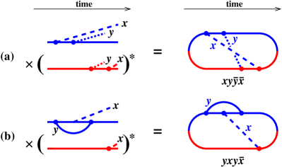
Figure 1: Two examples (previously computed 2brem ; qcd ) of interference contributions to the rates for (a) double splitting $g{\to}ggg$ and (b) virtual corrections to $g{\to}gg$ (where $y$ is virtual and must be integrated over). All lines in these diagrams represent high-energy gluons which implicitly and repeatedly interact with the medium (not shown). The left side above depicts contributions to the rate, obtained by multiplying a contribution to the amplitude (blue) by a contribution to the conjugate amplitude (red), with a particular time-ordering of all the vertices. The right side shows a more compact way of diagrammatically representing the same interference contributions, which is particularly useful for our implementation and extension 2brem ; qcd of Zakharov’s method Zakharov1 ; Zakharov2 for organizing and computing the LPM effect. In these diagrams, we need not follow a daughter of the splitting after its emission has occurred in both the amplitude and conjugate amplitude because we will only consider $p_{\perp}$-integrated rates. (See, for example, section 4.1 of ref. 2brem for an explicit argument.) The (time-ordered) diagrams are named $xy\bar{y}\bar{x}$ and $xyy\bar{x}$ here according to the convention of refs. 2brem ; qcd , summarized in the text.

Missing from that analysis were diagrams involving exchange of a longitudinally-polarized gluon in lightcone gauge. As we’ll review later, such interactions are instantaneous in lightcone time. Examples are shown in fig. 2, where we follow the standard LCPT convention of using a vertical line (because the interaction is instantaneous) crossed by a bar to represent the longitudinally-polarized gluon. Analogous contributions to overlap effects in double splitting have previously been analyzed for large-$N_{\rm f}$ QED in ref. QEDnf , and we will use similar methods here.

Also missing from the “nearly complete” calculation of ref. qcd were processes involving the fundamental 4-gluon interactions of QCD, examples of which are shown in fig. 3. Ref. 4point previously computed such processes in the case of real double splitting $g{\to}ggg$, such as fig. 3a, but the corresponding virtual diagrams, such as fig. 3b, have not previously been calculated.

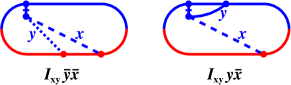
Figure 2: Two examples of interference contributions involving a longitudinally polarized gluon, represented by the vertical line crossed by a bar. The line is drawn vertically because the interaction is instantaneous in (lightcone) time.

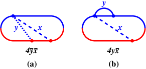
Figure 3: Two examples of interference contributions involving a fundamental 4-gluon vertex: (a) example of double splitting contributions $g{\to}ggg$ calculated in ref. 4point , and (b) example of a corresponding virtual diagram to be computed in this paper.

The goal of this paper, then, is to analyze all remaining gluonic QCD diagrams. These involve either (i) instantaneous longitudinal gluon exchange in LCPT or (ii) fundamental 4-gluon vertices. A complete list of such diagrams is depicted by figs. 4–6, plus additionally diagrams obtained by replacing $x{\to}1{-}x$ in fig. 5. Each circular blob in the diagrams represents the sum of a fundamental 4-gluon vertex plus all possible channels for a longitudinal gluon exchange, as depicted in fig. 7.

Figure 4: Diagrams for real double splitting $g{\to}ggg$ that involve an instantaneous exchange or fundamental 4-gluon interaction. See fig. 7 for the meaning of the large circular blob. The diagram drawn on a gray background turns out to be exactly zero.

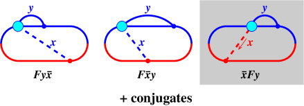
Figure 5: Like fig. 4 but for Class I virtual corrections to single splitting $g{\to}gg$. Our terminology “Class I” qcd means that (i) $y$ should be integrated over $0<y<1{-}x$ for these diagrams and (ii) $x\to 1{-}x$ generates another, distinct set of diagrams.

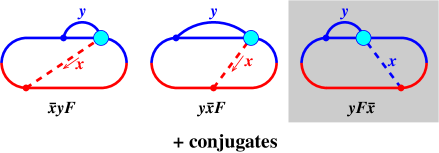
Figure 6: Like figs. 4 and 5 but for Class II virtual corrections to single splitting $g{\to}gg$. Our terminology “Class II” qcd means that (i) $y$ should be integrated over $0<y<1$ for these diagrams and (ii) the diagrams are symmetric under $x\to 1{-}x$.

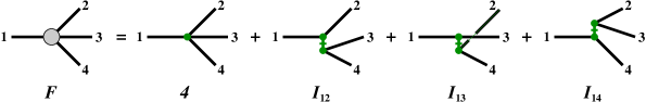
Figure 7: The meaning of the circular blob (“F”) in terms of the fundamental 4-gluon vertex (“4”) and LCPT instantaneous longitudinal gluon exchange in various channels (${\rm I}_{12}$, ${\rm I}_{13}$, ${\rm I}_{14}$). The green color here has no meaning other than to highlight the interactions that make up the circular blob.

In naming time-ordered diagrams, such as $xy\bar{y}\bar{x}$ in fig. 1a, we follow refs. 2brem ; qcd and refer to the gluons in order of the time when they were emitted. The absence or presence of a bar over a letter indicates whether the emission at that time was in the amplitude or conjugate amplitude. As in fig. 7, we will use “4” to denote a fundamental 4-gluon vertex and use “I” to denote an instantaneous exchange of a longitudinal gluon in LCPT. Effectively, these are both different types of four-point interactions of transversely-polarized gluons. When combined together, as in the circular blobs of figs. 4–7, we will refer to sum with the letter “F,” which is intended to evoke the word “four.”

It’s worth noting that there are two different types of processes where instantaneous longitudinal gluon exchange plays a role in figs. 4–6. One is by mediating $1{\to}3$ gluon pair creation processes as in fig. 2. All of the instantaneous vertices included in figs. 4 and 5 are of this type. Because of the compact way the diagrams are drawn, this may not be visually obvious in some cases, such as the $\bar{y}F\bar{x}$ diagram of fig. 4, but the interpretation can be clarified by redrawing the diagrams as a product of an amplitude and conjugate amplitude, as in fig. 8a. In contrast, the instantaneous vertices included in fig. 6 represent $2{\to}2$ final-state rescattering corrections (via longitudinal gluon exchange) to the leading-order $g{\to}gg$ single-splitting process, as depicted for $\bar{x}yF$ in fig. 8b.

Figure 8: Specific examples of instantaneous diagrams (depicted here in just one of the three possible channels) that are included in the (a) $\bar{y}F\bar{x}$ diagram of fig. 4 and (b) $\bar{x}yF$ diagram of fig. 6.

1.2 Assumptions and Simplifications

We will make the same simplifying assumptions made for other diagrams in ref. qcd (and throughout the program of refs. 2brem ; seq ; dimreg ; 4point ; QEDnf ; qedNfstop ; qcd for treating overlaps of successive hard splittings). We work in the theorist’s limit of an infinite, static, homogeneous QCD medium. In this context, we take the high-energy limit and make the corresponding high-energy approximation that the relevant interactions with the medium can be described by the medium parameter $\hat{q}$, defined as the proportionality constant in the formula $\langle p_{\perp}^{2}\rangle=\hat{q}L$ for the typical $p_{\perp}$ picked up by a high-energy particle traversing distance $L$ in the medium (for $L$ large compared to the mean-free path for scattering from the medium). We formally treat the running coupling $\alpha_{\rm s}(\mu)$ as small at scales associated with the splitting vertices for high-energy particles. Throughout, we will only consider rates that have been integrated over the transverse momenta $p_{\perp}$ of the final-state daughters of the $g{\to}ggg$ or $g{\to}gg$ splitting process. We will also work in the large-$N_{\rm c}$ limit (where $N_{\rm c}$ is the number of colors), which drastically simplifies color dynamics for the overlap calculation.

1.3 Outline

Our strategy in this paper will be to first, in section 2, evaluate the real double-splitting $g{\to}ggg$ diagrams of fig. 4 by adapting the calculations of ref. 4point , which were for those diagrams that have fundamental 4-gluon vertices. In section 3, we then transform those $g{\to}ggg$ results to obtain results for the virtual diagrams of figs. 5 and 6 by using the diagrammatic techniques of “front-end” and “back-end” transformations that were developed in ref. QEDnf in the context of large-$N_{\rm f}$ QED and later applied to gluon splitting processes in ref. qcd . A detailed summary of our final formulas for the effect of overlapping formation times on splitting rates is given in appendix A, in a format allowing easy integration with the earlier “nearly-complete” results of ref. qcd . The goal of this paper is merely to obtain formulas for the relevant rates. Our short conclusion in section 4 briefly references where one must go from here to evaluate the relative importance of the new contributions.

2 $g{\to}ggg$ processes with instantaneous interactions

2.1 The $F\bar{y}\bar{x}$ diagram

For a concrete start, we now discuss how to generalize earlier results for the $4\bar{y}\bar{x}$ interference diagram of fig. 3a to include instantaneous diagrams and so obtain the more general $F\bar{y}\bar{x}$ diagram of fig. 4.

2.1.1 Large-$N_{\rm c}$ color routings

One effect of taking the large-$N_{\rm c}$ limit to simplify color dynamics is that certain types of interference diagrams get contributions from more than one way to route large-$N_{\rm c}$ color in those diagram seq ; 4point . A simple way to picture different large-$N_{\rm c}$ color routings for a time-ordered diagram is (following refs. seq ; 4point ) to draw the diagram without crossing lines on a cylinder, where time runs along the length of the cylinder. Fig. 9a, adapted from ref. 4point , gives one example for the $4\bar{y}\bar{x}$ diagram. There is a different large-$N_{\rm c}$ color routing for each different way you can choose which high-energy particles neighbor each other as one circles around the circumference of the cylinder. There are exactly two different possibilities for the $4\bar{y}\bar{x}$ diagram, both shown in fig. 9. We must separately analyze these color routings because the medium-averaged interactions of the high-energy particles with the medium during 4-particle evolution (the gray region) is different in the two case. That’s because, in the large-$N_{\rm c}$ limit, medium interactions of gluon lines are correlated only between neighbors.

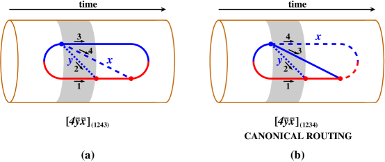
Figure 9: The two large-$N_{\rm c}$ color routings of the $4\bar{y}\bar{x}$ diagram, drawn on a time-ordered cylinder. These particular diagrams are drawn completely on the front side of the cylinder. The shaded region shows the times where four particles are present in the interference diagram (three in the amplitude plus one in the conjugate amplitude). Numbering of the lines in that region is according to the convention (1).

Following earlier work, we number the lines in these figures according to the longitudinal momentum fractions of the lines as

$$(x_{1},x_{2},x_{3},x_{4})=(-1,y,1{-}x{-}y,x).$$ (1)

With this convention, the order of particles going around the cylinder in the gray (4-particle evolution) section of fig. 9b is (1234), which means that any pair of particles are neighbors except for the pairs 1,3 and 2,4. In contrast, the particle order for fig. 9a is (1243). The contributions of these two color routings of $4\bar{y}\bar{x}$ to the differential rate $d\Gamma/dx\,dy$ are related to each other by simply interchanging $x_{3}\leftrightarrow x_{4}$, which is equivalent to $x\to 1{-}x{-}y$. It’s our custom to refer to the routing (1234) as our “canonical” routing in this context and then obtain the result for the other routing by substitution. Henceforth, we’ll refer to the contribution to the rate from a canonical routing as $[d\Gamma/dx\,dy]^{\rm canon}$. So, for the $4\bar{y}\bar{x}$ diagram,

$$\left[\frac{d\Gamma}{dx\,dy}\right]_{4\bar{y}\bar{x}}=\left[\frac{d\Gamma}{dx\,dy}\right]_{4\bar{y}\bar{x}}^{\rm canon}+~{}(x\to 1{-}x{-}y).$$ (2)

Let’s now do the same but also include instantaneous diagrams:

$$\left[\frac{d\Gamma}{dx\,dy}\right]_{F\bar{y}\bar{x}}=\left[\frac{d\Gamma}{dx\,dy}\right]_{F\bar{y}\bar{x}}^{\rm canon}+~{}(x\to 1{-}x{-}y).$$ (3)

The complete set of 4-point plus instantaneous color-routed diagrams that can contribute to the canonical color routing (1234) is shown on the cylinder in fig. 10. In the diagram labels, we have not written a “canon” subscript on “$I_{14}\bar{y}\bar{x}$” because there is only one possible large-$N_{\rm c}$ color routing of that particular time-ordered diagram — the canonical one. There is no way to obtain the canonical large-$N_{\rm c}$ color routing using $I_{13}$.

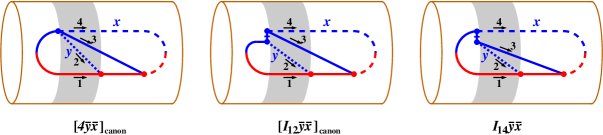
Figure 10: Like fig. 9b but here including all instantaneous diagrams that contribute to the canonical routing (1234) and so to $[d\Gamma/dx\,dy]_{F\bar{y}\bar{x}}^{\rm canon}$.

2.1.2 Diagrammatic rule for longitudinal gluon exchange

The $4\bar{y}\bar{x}$ diagram was previously calculated in ref. 4point . To evaluate the other diagrams of fig. 10, we will leverage the previous result by only computing in this paper the relative overall factors of the three diagrams. Then we will adjust the overall factor of the earlier $4\bar{y}\bar{x}$ result correspondingly. The relative factors include the effects of helicity contractions, color contractions, and longitudinal momentum fraction ($x_{i}$) dependence associated with the different four-gluon interactions $F$ in the different diagrams of fig. 10. Everything else about the diagrams (the 3-gluon vertices, the evolution of the high-energy particles in the medium) is the same.

The easiest way to compare the different four-gluon interactions is to forget about time-ordered perturbation theory for a moment and just think about Feynman rules. These are shown for light-cone gauge $A^{+}{=}0$ in fig. 11, where we follow our convention that unbarred lines represent transversely polarized gluons and the barred line represents a longitudinally polarized gluon. One may take the rule for longitudinal gluon exchange from the literature. But, since some of the LCPT literature has confusing normalization or sign issues, we will take a moment here to briefly review the derivation.

Figure 11: Ordinary Feynman rule results in lightcone gauge for the four-gluon interactions appearing in our “$F$” diagrams. By ordinary Feynman rules, we mean that (i) there is no direction of time in the above diagrams, (ii) we are not yet taking the large-$N_{\rm c}$ limit nor yet separating out different large-$N_{\rm c}$ color routings, and (iii) we are only talking about the interaction in an amplitude and are not thinking here about the conjugate amplitude. As in the rest of the text, unbarred lines refer to transversely polarized gluons, and the barred line is a longitudinally polarized gluon. $(a,b,c,d)$ are the adjoint-index colors of gluons $(1,2,3,4)$ respectively, and $(h_{1},h_{2},h_{3},h_{4})$ are the corresponding helicities $\pm$ flowing in the direction of the arrows. The Kronecker deltas arise from dot products ${\bm{\epsilon}}_{i}\cdot{\bm{\epsilon}}_{j}=\delta_{h_{i},-h_{j}}$ of the two-dimensional unit polarization vectors of (5).

In lightcone gauge, the basis $\epsilon_{(\lambda)}$ for transverse polarizations of a gauge boson with 4-momentum $p$ is given by

$$(\epsilon^{+},\epsilon^{-},{\bm{\epsilon}})_{(\lambda)}=\Bigl{(}0,\frac{{\bm{\epsilon}}_{(\lambda)}\cdot{\bm{p}}}{p^{+}},{\bm{\epsilon}}_{(\lambda)}\Bigr{)},$$ (4)

where ${\bm{\epsilon}}_{(\lambda)}$ is any basis of unit spatial vectors for the $xy$-plane. For a helicity basis, one may choose, for example,

$${\bm{\epsilon}}_{(\pm)}=\bigl{(}\tfrac{1}{\sqrt{2}},\pm\tfrac{i}{\sqrt{2}}\bigr{)}.$$ (5)

Here and throughout, boldface letters like ${\bm{\epsilon}}$ and ${\bm{p}}$ will denote the projection of vectors onto the $xy$-plane. Our convention for lightcone coordinates is that $v^{\pm}\equiv(v^{0}\pm v^{3})/\sqrt{2}$. So the 4-vector dot product [in $({+}{-}{-}{-})$ metric convention] is $u\cdot v=u^{+}v^{-}+u^{-}v^{+}-{\bm{u}}\cdot{\bm{v}}$, and $v_{\pm}=v^{\mp}$. The longitudinal polarization is

$$(\epsilon^{+},\epsilon^{-},{\bm{\epsilon}})_{\rm L}=(0,1,{\bm{0}}).$$ (6)

All three 4-vector basis polarizations are orthogonal to each other. The transverse polarizations are furthermore orthogonal to 4-vector $p$ and normalized so that $(\epsilon_{(\lambda)}^{*})^{\mu}(\epsilon_{(\lambda^{\prime})})_{\mu}=-\delta_{\lambda\lambda^{\prime}}$.

The lightcone gauge propagator is (ignoring $i\varepsilon$ prescriptions for now)

$$G^{\mu\nu}(q)=-\frac{i}{q^{2}}\Bigl{[}g^{\mu\nu}-\frac{q^{\mu}n^{\nu}+q^{\nu}n^{\mu}}{q\cdot n}\Bigr{]},$$ (7)

where it’s convenient to rewrite lightcone gauge $A^{+}=0$ as $n\cdot A=0$ with $(n^{+},n^{-},{\bm{n}})=(0,1,{\bm{0}})$. The propagator (7) may be recast into the form

$$G^{\mu\nu}(q)=G^{\mu\nu}_{\rm T}(q)+G^{\mu\nu}_{\rm L}(q)$$ (8a)

with

$$G^{\mu\nu}_{\rm T}(q)=\frac{i}{q^{2}}\sum_{\lambda}\epsilon_{(\lambda)}^{\mu}(q)\,\epsilon_{(\lambda)}^{\nu*}(q),\qquad G^{\mu\nu}_{\rm L}(q)=\frac{i}{(q\cdot n)^{2}}\,n^{\mu}n^{\nu}.$$ (8b)

Note that $q\cdot n=q^{+}$.

The rule for the longitudinally polarized gluon exchange in fig. 11 comes from applying normal Feynman rules but including only the longitudinal piece $G_{\rm L}$ of the lightcone propagator for the exchanged gluon. The result that this rule is independent of any $p^{-}$ is the reason why (after Fourier transformation to coordinate space) the interaction is instantaneous in lightcone time $x^{+}$. It is also local in ${\bm{x}}\equiv(x^{1},x^{2})$ but is non-local in $x^{-}$.

2.1.3 The color routings and contractions for fig. 10

Now turn to the large-$N_{\rm c}$, canonically routed diagrams of fig. 10. In our convention for defining the flow of momenta there, all of the arrows flow away from the four-gluon interaction in the amplitude, matching the flow convention of fig. 11. Note that the fundamental 4-point vertex in fig. 11 can be written as

$$-ig^{2}\Bigl{\{}\tfrac{1}{2}f^{abe}f^{cde}(\delta_{h_{1},-h_{3}}\delta_{h_{2},-h_{4}}-\delta_{h_{1},-h_{4}}\delta_{h_{2},-h_{3}})+f^{ade}f^{bce}(\delta_{h_{1},-h_{2}}\delta_{h_{3},-h_{4}}-\delta_{h_{1},-h_{3}}\delta_{h_{2},-h_{4}})\Bigr{\}}\\ +(\mbox{interchange particles 3 and 4}),$$ (9)

and remember that the two different color routings of the $4\bar{y}\bar{x}$ diagram are related by interchange of particles 3 and 4. In ref. 4point , the piece of our (9) that contributes to the canonical large-$N_{\rm c}$ color routing of the $4\bar{y}\bar{x}$ diagram in fig. 10 was found to be the first term in (9):

$$[4\bar{y}\bar{x}]_{\rm canon}\propto-ig^{2}\Bigl{\{}\tfrac{1}{2}f^{abe}f^{cde}(\delta_{h_{1},-h_{3}}\delta_{h_{2},-h_{4}}-\delta_{h_{1},-h_{4}}\delta_{h_{2},-h_{3}})\\ +f^{ade}f^{bce}(\delta_{h_{1},-h_{2}}\delta_{h_{3},-h_{4}}-\delta_{h_{1},-h_{3}}\delta_{h_{2},-h_{4}})\Bigr{\}}.$$ (10)

If one ignored color routing, the $I_{12}$ interaction of $I_{12}\bar{y}\bar{x}$ would give

$$ig^{2}f^{abe}f^{cde}\delta_{h_{1},-h_{2}}\delta_{h_{3},-h_{4}}\,\frac{(p_{1}^{+}-p_{2}^{+})(p_{3}^{+}-p_{4}^{+})}{(p_{1}^{+}+p_{2}^{+})^{2}}.$$ (11)

This single term is symmetric under exchange of particles 3 and 4, and we find that each large-$N_{\rm c}$ color routing corresponds to half of it:

$$[I_{12}\bar{y}\bar{x}]_{\rm canon}\propto\tfrac{1}{2}\,ig^{2}f^{abe}f^{cde}\delta_{h_{1},-h_{2}}\delta_{h_{3},-h_{4}}\,\frac{(p_{1}^{+}-p_{2}^{+})(p_{3}^{+}-p_{4}^{+})}{(p_{1}^{+}+p_{2}^{+})^{2}}.$$ (12a)

Finally, there is no color routing issue for the $$I_{14}\bar{y}\bar{x} I_{12} I_{14}$$ diagram, so we can convert the full (11) for to by switching the labels of particles 2 and 4:

$$I_{14}\bar{y}\bar{x}\propto ig^{2}f^{ade}f^{cbe}\delta_{h_{1},-h_{4}}\delta_{h_{3},-h_{2}}\,\frac{(p_{1}^{+}-p_{4}^{+})(p_{3}^{+}-p_{2}^{+})}{(p_{1}^{+}+p_{4}^{+})^{2}}.$$ (12b)

Eqs. (10) and (12) are the only differences in the evaluation of the three diagrams of fig. 10. We’ll find it convenient later on in this paper to have introduced some short-hand notation for the various factors in these equations:

$$c_{12}\equiv f^{abe}f^{cde},\quad c_{13}\equiv f^{ace}f^{dbe},\quad c_{14}\equiv f^{ade}f^{bce};$$ (13a)

$$h_{12}\equiv\delta_{h_{1},-h_{2}}\delta_{h_{3},-h_{4}},\quad h_{13}\equiv\delta_{h_{1},-h_{3}}\delta_{h_{2},-h_{4}},\quad h_{14}\equiv\delta_{h_{1},-h_{4}}\delta_{h_{2},-h_{3}};$$ (13b)

$$i_{12}\equiv\frac{(x_{1}{-}x_{2})(x_{3}{-}x_{4})}{(x_{1}{+}x_{2})^{2}}\,,\quad i_{13}\equiv\frac{(x_{1}{-}x_{3})(x_{4}{-}x_{2})}{(x_{1}{+}x_{3})^{2}}\,,\quad i_{14}\equiv\frac{(x_{1}{-}x_{4})(x_{2}{-}x_{3})}{(x_{1}{+}x_{4})^{2}}\,,$$ (13c)

where the $x_{n}$ are the $p^{+}$ momentum fractions defined by $p_{n}^{+}\equiv x_{n}P^{+}$, where $P$ is the 4-momentum of the initial particle in the double-splitting process. With this notation, the relative factors that differ between the three diagrams are

$$[4\bar{y}\bar{x}]_{\rm canon} \propto-\tfrac{1}{2}c_{12}(h_{13}-h_{14})-c_{14}(h_{12}-h_{13}),$$ (14a)

$$[I_{12}\bar{y}\bar{x}]_{\rm canon} \propto\tfrac{1}{2}c_{12}h_{12}i_{12},$$ (14b)

$$I_{14}\bar{y}\bar{x} \propto c_{14}h_{14}i_{14},$$ (14c)

where we’ve now absorbed the common factor of $ig^{2}$ into the joint proportionality.

For future reference, note that the $c_{1n}$ and $i_{1n}$ have been defined in such a way that $(c_{12},c_{13},c_{14})$ and $(i_{12},i_{13},i_{14})$ cyclically permute when the particle labels $(234)$ are cyclically permuted. However, the definitions pick up an additional minus sign when swapping just one pair of particle labels. For example, swapping particles 2 and 4 takes $(c_{12},c_{13},c_{14})\rightarrow(-c_{14},-c_{13},-c_{12})$ and $(i_{12},i_{13},i_{14})\rightarrow(-i_{14},-i_{13},-i_{12})$ and so takes $(c_{12}i_{12},c_{13}i_{13},c_{14}i_{14})\rightarrow(c_{14}i_{14},c_{13}i_{13},c_{12}i_{12})$.

In the calculation of rates, we will sum/average over final/initial state helicities and colors, as we did for $[4\bar{y}\bar{x}]_{\rm canon}$ alone in ref. 4point . To compare the relative rates among our diagrams here, we now need to be explicit about what common factors hidden in the common proportionality symbols depend on colors and helicities.

Let’s start by first focusing on color. The color factors from the two 3-gluon vertices in the $F\bar{y}\bar{x}$ diagrams of fig. 10 are proportional to $f^{abf}f^{cdf}=c_{12}$. (Proportionality is enough here. Since they are the same for all three diagrams, we do not have to keep track of the appropriate order of the indices in the 3-gluon vertex $f$’s because that only affects the common overall sign of those diagrams.) Letting angle brackets $\langle\cdots\rangle$ represent summing/averaging over colors in this particular context, one finds

$$\langle c_{12}c_{12}\rangle=C_{\rm A}^{2},\qquad\langle c_{12}c_{13}\rangle=\langle c_{12}c_{14}\rangle=-\tfrac{1}{2}C_{\rm A}^{2}.$$ (15)

We then have

$$[4\bar{y}\bar{x}]_{\rm canon} \propto-\tfrac{1}{2}\langle c_{12}c_{12}\rangle(h_{13}-h_{14})-\langle c_{12}c_{14}\rangle(h_{12}-h_{13})\propto h_{12}-2h_{13}+h_{14},$$ (16a)

$$[I_{12}\bar{y}\bar{x}]_{\rm canon} \propto\tfrac{1}{2}\langle c_{12}c_{12}\rangle h_{12}i_{12}\propto h_{12}i_{12},$$ (16b)

$$I_{14}\bar{y}\bar{x} \propto\langle c_{12}c_{14}\rangle h_{14}i_{14}\propto-h_{14}i_{14},$$ (16c)

where we’ve absorbed a common factor of $\tfrac{1}{2}C_{\rm A}^{2}$ into the second proportionality symbol of each line.

2.1.4 Helicity contractions

We now need to include the helicity dependence of the two 3-gluon vertices and then sum/average over helicity. In the notation of refs. 2brem ; 4point , the 3-gluon vertices give factors of

$$\Bigl{[}\sum_{\bar{h}}{\cal P}^{\bar{m}}_{h_{\rm i}\to\bar{h},h_{\rm y}}\!\bigl{(}1\to 1{-}y,y\bigr{)}\,{\cal P}^{\bar{n}}_{\bar{h}\to h_{\rm z},h_{\rm x}}\!\bigl{(}1{-}y\to 1{-}x{-}y,x\bigr{)}\,\Bigr{]}^{*},$$ (17)

where the ${\cal P}$ are given in terms of square roots of helicity-dependence vacuum Dokshitzer-Gribov-Lipatov-Altarelli-Parisi (DGLAP) splitting functions. The exact definitions can be found in ref. 2brem , where $\bm{\mathcal{P}}$ is defined as a 2-dimensional vector proportional to $(1,+i)$ or $(1,-i)$ depending on the specific helicity transition. The indices $\bar{m}$ and $\bar{n}$ in (17) index the components of that vector. $h_{\rm i}$ is the helicity of the initial particle in the $g{\to}ggg$ splitting process; $(h_{\rm x},h_{\rm y},h_{\rm z})$ are the helicities of the three daughters; and $\bar{h}$ is the helicity of the unlabeled red line connecting the two 3-gluon vertices in each of the three diagrams of fig. 10. With the numbering and flow direction conventions of the lines in fig. 10, (17) is

$$\Sigma^{\bar{m}\bar{n}}\equiv\Bigl{[}\sum_{\bar{h}}{\cal P}^{\bar{m}}_{-h_{1}\to\bar{h},h_{2}}\!\bigl{(}1\to 1{-}y,y\bigr{)}\,{\cal P}^{\bar{n}}_{\bar{h}\to h_{3},h_{4}}\!\bigl{(}1{-}y\to 1{-}x{-}y,x\bigr{)}\,\Bigr{]}^{*}.$$ (18)

Now let’s sum/average over the daughter and parent helicities. We’ll denote that helicity sum/average using angle brackets as well. In ref. 4point , the relevant average for the $4\bar{y}\bar{x}$ diagram was found to be (using our notation here)

$$\bigl{\langle}\Sigma^{\bar{m}\bar{n}}\,(h_{12}-2h_{13}+h_{14})\bigr{\rangle}\,|x_{1}x_{2}x_{3}x_{4}|^{-1/2}=\zeta_{(4)}(x,y)\,\delta^{\bar{m}\bar{n}}$$ (19)

with

$$\zeta_{(4)}(x,y)=\frac{2x^{2}-z^{2}-(1{-}y)^{4}+2y^{2}z^{2}-x^{2}y^{2}}{(xyz)^{2}(1{-}y)^{3}}\,.$$ (20)

By repeating that calculation, we find now that the separate pieces of (19) are given by

$$\langle\Sigma^{\bar{m}\bar{n}}\,h_{1k}\rangle\,|x_{1}x_{2}x_{3}x_{4}|^{-1/2}=\zeta_{1k}(x,y)\,\delta^{\bar{m}\bar{n}}$$ (21)

with

$$\zeta_{12} =\frac{(x^{2}{+}z^{2})(1{+}y^{2})}{(xyz)^{2}(1{-}y)^{3}}\,,$$ (22a)

$$\zeta_{13} =\frac{(1{-}y)^{4}+z^{2}+x^{2}y^{2}}{(xyz)^{2}(1{-}y)^{3}}\,,$$ (22b)

$$\zeta_{14} =\frac{(1{-}y)^{4}+x^{2}+z^{2}y^{2}}{(xyz)^{2}(1{-}y)^{3}}\,,$$ (22c)

in terms of which

$$\zeta_{(4)}=\zeta_{12}-2\zeta_{13}+\zeta_{14}.$$ (23)

So, after helicity summing/averaging, (16) becomes

$$[4\bar{y}\bar{x}]_{\rm canon} \propto\bigl{\langle}\Sigma^{\bar{m}\bar{n}}\,(h_{12}-2h_{13}+h_{14})\bigr{\rangle}\propto\zeta_{(4)}\,\delta^{\bar{m}\bar{n}},$$ (24a)

$$[I_{12}\bar{y}\bar{x}]_{\rm canon} \propto\langle\Sigma^{\bar{m}\bar{n}}\,h_{12}\rangle\,i_{12}\propto\zeta_{12}\,i_{12}\,\delta^{\bar{m}\bar{n}},$$ (24b)

$$I_{14}\bar{y}\bar{x} \propto-\langle\Sigma^{\bar{m}\bar{n}}\,h_{14}\rangle\,i_{14}\propto-\zeta_{14}\,i_{14}\,\delta^{\bar{m}\bar{n}}.$$ (24c)

From this, we see that the result for $4\bar{y}\bar{x}$ in ref. 4point can be converted to a result for $F\bar{y}\bar{x}$ (which includes instantaneous diagrams) by

$$\left[\frac{d\Gamma}{dx\,dy}\right]_{F\bar{y}\bar{x}}^{\rm canon}=\left\{\left[\frac{d\Gamma}{dx\,dy}\right]_{4\bar{y}\bar{x}}^{\rm canon}~{}\mbox{with}~{}\zeta_{(4)}\longrightarrow\zeta_{\rm(F)}\right\},$$ (25)

where

$$\zeta_{\rm(F)}=\zeta_{(4)}+\zeta_{12}\,i_{12}-\zeta_{14}\,i_{14}=\zeta_{(4)}-\frac{(1{+}y)(z{-}x)}{(1{-}y)^{2}}\,\zeta_{12}-\frac{(1{+}x)(z{-}y)}{(1{-}x)^{2}}\,\zeta_{14}.$$ (26)

We summarize the final formulas for this and all other rates involving 4-gluon interactions in appendix A.

2.1.5 The $\bar{y}\bar{x}F$ and $\bar{y}F\bar{x}$ diagrams

The color and helicity sums for the $\bar{y}\bar{x}F$ diagram are the same as those for the $F\bar{y}\bar{x}$ diagram, and so the same substitution $\zeta_{(4)}\to\zeta_{(F)}$ as in (25) can be made on the result for the canonical routing (1234) of $\bar{y}\bar{x}4$ from ref. 4point .

The $\bar{y}F\bar{x}$ diagram vanishes for the same reason as the $\bar{y}4\bar{x}$ diagram in ref. 4point , which can be argued from parity invariance of either the initial or final 3-particle evolution in this diagram. (See section 3.2 of ref. 4point .)

2.2 The $F\bar{F}$ diagram

There are three large-$N_{\rm c}$ color routings of the $4\bar{4}$ diagram, shown in fig. 12. Again, we choose the “canonical” routing to be the one ordered (1234) according to (1). The total $4\bar{4}$ contribution can then be written

$$\left[\frac{d\Gamma}{dx\,dy}\right]_{4\bar{4}}=\left[\frac{d\Gamma}{dx\,dy}\right]_{4\bar{4}}^{\rm canon}+~{}[(x,y,z)\rightarrow(z,y,x)]~{}+~{}[(x,y,z)\rightarrow(z,x,y)],$$ (27)

where here $x$, $y$, and $z\,{\equiv}\,1{-}x{-}y$ represent the three daughters of the $g\to ggg$ splitting process. We now generalize to include instantaneous diagrams by writing

$$\left[\frac{d\Gamma}{dx\,dy}\right]_{F\bar{F}}=\left[\frac{d\Gamma}{dx\,dy}\right]_{F\bar{F}}^{\rm canon}+~{}[(x,y,z)\rightarrow(z,y,x)]~{}+~{}[(x,y,z)\rightarrow(z,x,y)].$$ (28)

The diagrams which contribute to the canonical routing (1234) are shown in fig. 13.

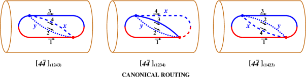
Figure 12: The three large-$N_{\rm c}$ color routings of the $4\bar{4}$ diagram, drawn with the same conventions as fig. 9 except that here we have not bothered to shade the region of 4-particle evolution. (This figure is adapted from fig. 14 of ref. 4point .)

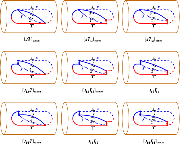
Figure 13: Like the middle diagram of fig. 12 but here also including all instantaneous diagrams that contribute to the canonical routing (1234) and so to $[d\Gamma/dx\,dy]_{F\bar{F}}^{\rm canon}$.

For the color and helicity factors, the simplest diagrams are those involving only longitudinally polarized gluon interactions, for which the factors [see fig. 11 and eqs. (13)] are

$$[I_{12}\,\bar{I}_{12}]_{\rm canon} \propto\tfrac{1}{2}|ig^{2}c_{12}h_{12}i_{12}|^{2},$$ (29a)

$$[I_{14}\,\bar{I}_{14}]_{\rm canon} \propto\tfrac{1}{2}|ig^{2}c_{14}h_{14}i_{14}|^{2},$$ (29b)

$$I_{12}\,\bar{I}_{14} \propto(ig^{2}c_{12}h_{12}i_{12})(ig^{2}c_{14}h_{14}i_{14})^{*},$$ (29c)

$$I_{14}\,\bar{I}_{12} \propto(ig^{2}c_{14}h_{14}i_{14})(ig^{2}c_{12}h_{12}i_{12})^{*},$$ (29d)

where the factors of $$\tfrac{1}{2} [4\,\bar{I}_{12}]_{\rm canon} [4\bar{y}\bar{x}]_{\rm canon} I_{12}$$ arise for diagrams that have two color routings when only one of those two routings is included in fig. 13. The diagrams involving the fundamental 4-gluon vertex are a little more subtle, but we can again leverage previous results. The color contractions and particle numbering in the diagram of fig. 13 are identical to those for the diagram discussed earlier. So, the appropriate piece of the 4-gluon vertex that contributes to this particular color routing will be the same as that quoted in (10), taken in turn from ref. 4point . Combining with the factors for in the conjugate amplitude then gives

$$[4\,\bar{I}_{12}]_{\rm canon}\propto\bigl{\{}-ig^{2}\bigl{[}\tfrac{1}{2}c_{12}(h_{13}{-}h_{14})+c_{14}(h_{12}{-}h_{13})\bigr{]}\bigr{\}}\,(ig^{2}c_{12}h_{12}i_{12})^{*}.$$ (29e)

Though maybe not at first obvious from the way the diagrams have been drawn, the $$[4\,\bar{I}_{14}]_{\rm canon} [4\,\bar{I}_{12}]_{\rm canon} 2 4 x\leftrightarrow y N_{\rm c} c_{1n} i_{1n} c_{12}\leftrightarrow-c_{14} i_{12}\leftrightarrow-i_{14}$$ diagram is the same as the diagram except for interchange of particles and (i.e. ). To see that the color routings are the same after that interchange, remember that it doesn’t matter whether one circles the cylinder one way and names the routing (1234) or circles the other way and names it in reverse order (1432). All that matters in the large- limit is which lines are neighbors going around the cylinder. So, by swapping particles 2 and 4 in (29e) while remembering that our definitions of and imply and under such a swap,

$$[4\,\bar{I}_{14}]_{\rm canon}\propto\bigl{\{}-ig^{2}\bigl{[}\tfrac{1}{2}c_{14}(h_{12}{-}h_{13})+c_{12}(h_{13}{-}h_{14})\bigr{]}\bigr{\}}\,(ig^{2}c_{14}h_{14}i_{14})^{*}.$$ (29f)

The color and helicity factors are insensitive to the time ordering of the vertices, and so the factors for $$[I_{12}\,\bar{4}]_{\rm canon} [I_{14}\,\bar{4}]_{\rm canon} [4\,\bar{I}_{12}]_{\rm canon} [4\,\bar{I}_{14}]_{\rm canon}$$ and are just the complex conjugates of those for and :

$$[I_{12}\,\bar{4}]_{\rm canon}\propto(ig^{2}c_{12}h_{12}i_{12})\bigl{\{}-ig^{2}\bigl{[}\tfrac{1}{2}c_{12}(h_{13}{-}h_{14})+c_{14}(h_{12}{-}h_{13})\bigr{]}\bigr{\}}^{*},$$ (29g)

$$[I_{14}\,\bar{4}]_{\rm canon}\propto(ig^{2}c_{14}h_{14}i_{14})\bigl{\{}-ig^{2}\bigl{[}\tfrac{1}{2}c_{14}(h_{12}{-}h_{13})+c_{12}(h_{13}{-}h_{14})\bigr{]}\bigr{\}}^{*}.$$ (29h)

This overall complex conjugation doesn’t actually make a difference, since the above are real-valued. Finally, there is the $$4\bar{4} 4\bar{4} N_{\rm c}$$ diagram, which has the three color routings shown in fig. 12. As discussed in ref. 4point , the contribution of each color routing is just one third of what the total would be if we naively ignored the necessity of splitting the diagram into different large- color routings. So,

$$[4\,\bar{4}]_{\rm canon}\propto\tfrac{1}{3}\Bigl{|}-ig^{2}\bigl{[}c_{14}(h_{12}{-}h_{13})+c_{12}(h_{13}{-}h_{14})+c_{13}(h_{14}{-}h_{12})\bigr{]}\Bigr{|}^{2}.$$ (29i)

Recall that we defined the $(c_{12},c_{13},c_{14})$ to cyclically permute under permutations of the indices $(234)$. So (15) gives

$$\langle c_{12}c_{12}\rangle=\langle c_{13}c_{13}\rangle=\langle c_{14}c_{14}\rangle=C_{\rm A}^{2},$$ (30a)

$$\langle c_{12}c_{13}\rangle=\langle c_{13}c_{14}\rangle=\langle c_{14}c_{12}\rangle=-\tfrac{1}{2}C_{\rm A}^{2}.$$ (30b)

From the definition (13b) of the $h_{1n}$, final/initial helicity summing/averaging gives

$$\langle h_{12}h_{12}\rangle=\langle h_{13}h_{13}\rangle=\langle h_{14}h_{14}\rangle=2,$$ (31a)

$$\langle h_{12}h_{13}\rangle=\langle h_{13}h_{14}\rangle=\langle h_{14}h_{12}\rangle=1.$$ (31b)

Eqs. (29) then yield (after absorbing a common factor of $C_{\rm A}^{2}g^{4}$ into the proportionality)

$$[I_{12}\,\bar{I}_{12}]_{\rm canon} \propto i_{12}^{2},$$ (32)

$$[I_{14}\,\bar{I}_{14}]_{\rm canon} \propto i_{14}^{2},$$ (33)

$$I_{12}\,\bar{I}_{14} \propto-\tfrac{1}{2}i_{12}i_{14},$$ (34)

$$I_{14}\,\bar{I}_{12} \propto-\tfrac{1}{2}i_{12}i_{14},$$ (35)

$$[4\,\bar{I}_{12}]_{\rm canon}=[I_{12}\,\bar{4}]_{\rm canon} \propto\tfrac{1}{2}i_{12},$$ (36)

$$[4\,\bar{I}_{14}]_{\rm canon}=[I_{14}\,\bar{4}]_{\rm canon} \propto-\tfrac{1}{2}i_{14},$$ (37)

$$[4\,\bar{4}]_{\rm canon} \propto 3.$$ (38)

Adding all nine color-routed diagrams of fig. 13 together,

$$[F\,\bar{F}]_{\rm canon}\propto 3+i_{12}^{2}+i_{14}^{2}-i_{12}i_{14}+i_{12}-i_{14},$$ (39)

to be compared with just $[4\,\bar{4}]_{\rm canon}\propto 3$. So, we can convert the result for $4\bar{4}$ in ref. 4point to the more general result for $F\bar{F}$ by

$$\left[\frac{d\Gamma}{dx\,dy}\right]_{F\bar{F}}^{\rm canon}=\bigl{[}1+\tfrac{1}{3}(i_{12}^{2}+i_{14}^{2}-i_{12}i_{14}+i_{12}-i_{14})\bigr{]}\left[\frac{d\Gamma}{dx\,dy}\right]_{4\bar{4}}^{\rm canon}.$$ (40)

A summary of the final rate formula is given in appendix A.

3 Virtual corrections to $g{\to}gg$ with 4-gluon interactions

3.1 Basic results

In previous work QEDnf ; qcd , we showed how almost all of the diagrams considered there for virtual corrections to single splitting $g{\to}gg$ could be simply related to diagrams for real double splitting $g{\to}ggg$ through what we call front- and/or back-end transformations. Those same techniques can be applied to all of the virtual diagrams of this paper. In particular, fig. 14 depicts graphically how the virtual diagrams of figs. 5 and 6 are related to the $g{\to}ggg$ diagrams of fig. 4. The front- and back-end transformations are represented by the black arrows in the bottom half of fig. 14. Graphically, front-end transformations correspond to sliding the earliest-time vertex in the interference diagram around the front end of the diagram from amplitude to conjugate amplitude or vice versa. Back-end transformation correspond to similarly sliding the latest-time vertex around the back end of the diagram. The transformations depicted by fig. 14 involve various combinations, as indicated, of front-end transformations, back-end transformations, complex conjugation, and swapping variable names $x\leftrightarrow y$.

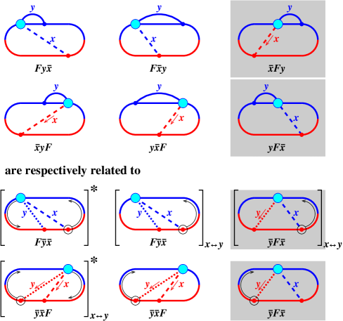
Figure 14: Relation of the virtual diagrams of figs. 5 and 6 to the real $g{\to}ggg$ diagrams of fig. 4 by various combinations of front- and back-end transformations, complex conjugation, and swapping variable names $x\leftrightarrow y$. Complex conjugation corresponds to flipping a diagram upside down and swapping the colors blue (amplitude) and red (conjugate amplitude). Complex conjugation is irrelevant, however, because ultimately we want to take $2\operatorname{Re}(\cdots)$ of all the virtual diagrams, i.e. add them to their complex conjugates. Shading above indicates diagrams that happen to be exactly zero, because the $\bar{y}F\bar{x}$ diagram vanishes for the reason described in section 2.1.5.

The simplest transformation is a back-end transformation, where the latest-time vertex changes sign because a $-i\,\delta H$ perturbation in the amplitude (from perturbing the evolution operator $e^{-iHt}$) moves to become a $+i\,\delta H$ perturbation in the conjugate amplitude (from perturbing $(e^{-iHt})^{*}=e^{+iHt}$), or vice versa. So fig. 14 tells us that

$$\left[\frac{d\Gamma}{dx}\right]_{F\bar{x}y}=-\tfrac{1}{2}\int_{0}^{1-x}dy\>\left\{\left[\frac{d\Gamma}{dx\,dy}\right]_{F\bar{y}\bar{x}}~{}\mbox{with}~{}x\leftrightarrow y\right\},$$ (41)

where the loop momentum fraction $y$ has been integrated over. The overall factor of $\tfrac{1}{2}$ is the symmetry factor of the (blue) loop in the amplitude of the $F\bar{x}y$ diagram in fig. 14.

Front-end transformations are similar, but the momentum fractions of the lines must be adjusted since they are defined relative to the parent energy $E$ of the entire splitting process, and which line is the parent changes under a front-end transformation. For the case $y\bar{x}F$ in fig. 14, where a $y$-emission 3-gluon vertex is being slid around the front of the diagram, this is

$$\left[\frac{d\Gamma}{dx}\right]_{y\bar{x}F}=-\tfrac{1}{2}\int_{0}^{1}dy\>\left\{\left[\frac{d\Gamma}{dx\,dy}\right]_{\bar{y}\bar{x}F}~{}\mbox{with}~{}(x,y,E)\longrightarrow\Bigl{(}\frac{x}{1{-}y}\,,\,\frac{{-}y}{1{-}y}\,,\,(1{-}y)E\Bigr{)}\right\}.$$ (42)

The sign change appearing in the transformation $y\to-y/(1{-}y)$ arises because our (very useful) convention 2brem is that particles in time-ordered interference diagrams have positive or negative momentum fractions depending on whether they are emitted first in the amplitude (blue lines) or conjugate amplitude (red lines), respectively.

For the $\bar{x}yF$ diagram in fig. 14, we combine the above transformation with a back-end transformation, conjugation, and $x\leftrightarrow y$:

$$\left[\frac{d\Gamma}{dx}\right]_{\bar{x}yF} =+\tfrac{1}{2}\int_{0}^{1}dy\>\Biggl{\{}\left[\frac{d\Gamma}{dx\,dy}\right]_{\bar{y}\bar{x}F}~{}\mbox{with}~{}(x,y,E)\longrightarrow\Bigl{(}\frac{x}{1{-}y}\,,\,\frac{{-}y}{1{-}y}\,,\,(1{-}y)E\Bigr{)}$$

$$\hskip 120.00018pt~{}\mbox{followed by}~{}x\leftrightarrow y\Biggr{\}}^{*}$$

$$=+\tfrac{1}{2}\int_{0}^{1}dy\>\left\{\left[\frac{d\Gamma}{dx\,dy}\right]_{\bar{y}\bar{x}F}~{}\mbox{with}~{}(x,y,E)\longrightarrow\Bigl{(}\frac{y}{1{-}x}\,,\,\frac{{-}x}{1{-}x}\,,\,(1{-}x)E\Bigr{)}\right\}^{*}.$$ (43)

For the case $Fy\bar{x}$, where the front-end transformation is of a 4-gluon interaction, the momentum fraction transformations are correspondingly different because the particle line that becomes the new parent is different, and also because the front-end transformation moves two emissions ($x$ and $y$) from amplitude to conjugate amplitude:

$$\left[\frac{d\Gamma}{dx\,dy}\right]_{Fy\bar{x}}=\\ +\tfrac{1}{2}\int_{0}^{1-x}dy\>\left\{\left[\frac{d\Gamma}{dx\,dy}\right]_{F\bar{y}\bar{x}}~{}\mbox{with}~{}(x,y,E)\longrightarrow\Bigl{(}\frac{{-}x}{1{-}x{-}y}\,,\,\frac{{-}y}{1{-}x{-}y}\,,\,(1{-}x{-}y)E\Bigr{)}\right\}^{*}.$$ (44)

3.2 Integrable infrared divergence from instantaneous interactions

Of all the various diagrams represented by figs. 4–6, there are four particular cases where divergences arise because the $q^{+}$ of an exchanged longitudinal gluon may become zero. Those cases are shown in fig. 15 and are all virtual diagrams corresponding to certain types of rescattering corrections to a leading-order single splitting $g{\to}gg$. The loop momentum fraction $y$ is integrated over $0<y<1$ in these diagrams, and the divergences occur at $y=1{-}x$ for the two diagrams in the top line of fig. 15 and at $y=x$ for the other two diagrams.

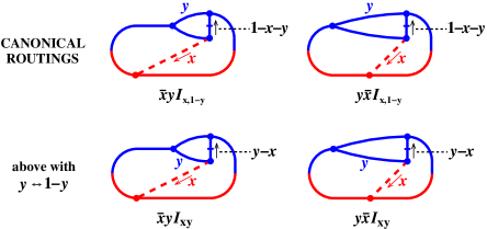
Figure 15: Diagrams with infrared divergences associated with longitudinally polarized gluon exchange. The divergences occur at either $y\to 1{-}x$ (top line) or $y\to x$ (bottom line).

In order to reduce the number of things to think about, we may focus on just the top line of fig. 15. These are the divergent contributions from $\bar{x}yF$ and $y\bar{x}F$ that are obtained by applying the relevant transformations (fig. 14) to only the canonical color routing of $\bar{y}\bar{x}F$. The other color routing of $\bar{y}\bar{x}F$ corresponds to swapping $x\leftrightarrow z$, which, after transformation, corresponds to swapping $y\leftrightarrow 1{-}y$ in $\bar{x}yF$ and $y\bar{x}F$. Since we are integrating $y$ over $0<y<1$ in these particular virtual diagrams, adding in the contribution from swapping $y\leftrightarrow 1{-}y$ is equivalent to multiplying the integral of the canonical routing by a factor of 2. So, we will rewrite (42) and (43) as

$$\left[\frac{d\Gamma}{dx}\right]_{y\bar{x}F} =-\int_{0}^{1}dy\>\left\{\left[\frac{d\Gamma}{dx\,dy}\right]_{\bar{y}\bar{x}F}^{\rm canon}~{}\mbox{with}~{}(x,y,E)\longrightarrow\Bigl{(}\frac{x}{1{-}y}\,,\,\frac{{-}y}{1{-}y}\,,\,(1{-}y)E\Bigr{)}\right\},$$ (45a)

$$\left[\frac{d\Gamma}{dx}\right]_{\bar{x}yF} =+\int_{0}^{1}dy\>\left\{\left[\frac{d\Gamma}{dx\,dy}\right]_{\bar{y}\bar{x}F}^{\rm canon}~{}\mbox{with}~{}(x,y,E)\longrightarrow\Bigl{(}\frac{y}{1{-}x}\,,\,\frac{{-}x}{1{-}x}\,,\,(1{-}x)E\Bigr{)}\right\}^{*}.$$ (45b)

Comparing to the earlier versions, notice the restriction “canon” now on the $\bar{y}\bar{x}F$ rates, and correspondingly the removal of the overall factors of $\tfrac{1}{2}$. The only divergences in the $y$ integration are now the ones at $y=1{-}x$, from the top line of fig. 15. Individually, each of the two diagrams in (45) has a $1/(1{-}x{-}y)^{2}$ divergence as $y\to 1{-}x$ because of the $1/(q^{+})^{2}=1/(p_{1}^{+}+p_{2}^{+})^{2}$ in fig. 11 associated with the propagator of the longitudinally polarized gluon.

In what follows, it will be convenient to get rid of the complex conjugation in (45b) by noting that ultimately these diagrams must be added to their complex conjugates, as noted at the bottom of fig. 6. It will also be convenient to add together all the diagrams (including the conjugates) of fig. 6. These diagrams represent the 4-gluon interaction contributions to a class of diagrams that were called “Class II” virtual diagrams in ref. qcd , and we adopt that nomenclature here for the sum. Remembering that the shaded diagram in fig. 6 is zero, we then have

$$\left[\frac{d\Gamma}{dx}\right]_{\rm F,~{}virt~{}II}=2\operatorname{Re}\left\{\left[\frac{d\Gamma}{dx}\right]_{y\bar{x}F}+\left[\frac{d\Gamma}{dx}\right]_{\bar{x}yF}\right\}=2\operatorname{Re}\int_{0}^{1}dy\>{\cal F}(x,y)$$ (46a)

with

$${\cal F}(x,y)\equiv -\left\{\left[\frac{d\Gamma}{dx\,dy}\right]_{\bar{y}\bar{x}F}^{\rm canon}~{}\mbox{with}~{}(x,y,E)\longrightarrow\Bigl{(}\frac{x}{1{-}y}\,,\,\frac{{-}y}{1{-}y}\,,\,(1{-}y)E\Bigr{)}\right\}$$

$$+\left\{\left[\frac{d\Gamma}{dx\,dy}\right]_{\bar{y}\bar{x}F}^{\rm canon}~{}\mbox{with}~{}(x,y,E)\longrightarrow\Bigl{(}\frac{y}{1{-}x}\,,\,\frac{{-}x}{1{-}x}\,,\,(1{-}x)E\Bigr{)}\right\}.$$ (46b)

Now that we’ve added the diagrams together and avoided any complex conjugation in (46b), it turns out that the $1/(1{-}x{-}y)^{2}$ divergences of the two terms cancel, leaving behind a milder $1/(1{-}x{-}y)$ divergence. To make our discussion more compact, we’ll loosely refer to this as a $1/z$ divergence with $z\equiv 1{-}x{-}y$. However, unlike the discussion of $g{\to}ggg$ processes in section 2, $z$ is not the momentum fraction of any final-state daughter of the single splitting processes being considered here, and $z$ need not be positive.

The nice thing about a $1/z$ divergence is that, since the integral $\int_{0}^{1}dy$ associated with the loop integrals of fig. 15 span both signs of $z=1{-}x{-}y$, the integral $\int dz/z$ will be finite: the divergent contributions from $z$ slightly negative will cancel those from $z$ slightly positive. Though the answer will be finite, the subtlety lies in figuring out what finite piece will be left over. We will address this first formally, and then as a practical matter to allow the $y$ integration in (46a) to be performed numerically in applications.

3.2.1 Disambiguation

Other diagrams in previous work qcd (which did not include longitudinally-polarized gluon exchange) had infrared divergences associated with one of the transversely polarized gluons becoming soft. There, we regulated those divergences by introducing a small infrared cut-off $\delta\ll 1$ on all momentum fractions such as $x$, $y$, $1{-}y$, etc. That’s equivalent to saying that we insisted that $p^{+}>(p^{+})_{\rm min}\equiv P^{+}\delta$, where $P$ is the momentum of the initial particle in the overlapping splitting process. In LCPT, the transversely polarized gluons all propagate forward in time with $p^{+}>0$. But there is no restriction on the longitudinally-polarized gluons, which have been integrated out and for which there is no forward direction of light-cone time since they mediate instantaneous interactions. Their $q^{+}$ can have either sign. One can regulate the magnitude of $q^{+}$ in a way consistent with the transversely polarized gluons: $|q^{+}|>(p^{+})_{\rm min}=P^{+}\delta$. Given that the infrared regulator $\delta$ is to be formally chosen as arbitrarily small, that’s equivalent to regulating our net $1/z$ divergence with a principal value (also known as principal part) prescription:

$$\operatorname{PV}\Bigl{[}\frac{1}{z}\Bigr{]}=\frac{\theta(|z|-\delta)}{z}\,,$$ (47)

where $\theta$ is the unit step function. In terms of $i\epsilon$ prescriptions, the principal value (PV) can alternatively be defined as

$$\operatorname{PV}\Bigl{[}\frac{1}{z}\Bigr{]}=\frac{1}{2}\left(\frac{1}{z-i\epsilon}+\frac{1}{z+i\epsilon}\right)=\frac{z}{z^{2}+\epsilon^{2}}\,.$$ (48)

Both (47) and (48) cut off small values of $z$ while keeping $\operatorname{PV}[1/z]$ real valued. The only difference is that one is a sharp IR cut-off on $|z|$ while the other is smoothed out.

The use of principle value prescriptions for such $1/q^{+}$ divergences in lightcone gauge had a convoluted early history Leibbrandt . Here, we rely on the more recent analysis by Chirilli, Kovchegov and Wertepny CKW ; CKWolder , which shows how various $i\epsilon$ prescriptions for $1/q^{+}$ divergences in lightcone gauge can be understood as corresponding to different sub-gauge choices of lightcone gauge and correspondingly to different choices of boundary conditions for gauge fields as $x^{-}\to\pm\infty$. Sub-gauges arise because the lightcone gauge condition $A^{+}{=}0$ does not by itself uniquely determine the gauge. In what they call PV sub-gauge, the Feynman propagator is

$$G^{\mu\nu}(q)=\frac{i}{q^{2}+i\epsilon}\,\Delta^{\mu\nu}(q)$$ (49a)

with

$$\Delta^{\mu\nu}(q)=-\biggl{\{}g^{\mu\nu}-(q^{\mu}n^{\nu}+q^{\nu}n^{\mu})\operatorname{PV}\Bigl{[}\frac{1}{q\cdot n}\Bigr{]}\biggr{\}}.$$ (49b)

They also explicitly check in certain examples the equivalence of calculations performed in different sub-gauges, one of which is PV sub-gauge.

For LCPT and for our calculation, we want to separate the transverse and longitudinal polarizations. Algebraically manipulating (49) into the form of (8) while maintaining the prescriptions gives

$$\Delta^{\mu\nu}(q)=\Delta_{\rm T}^{\mu\nu}(q)+\Delta_{\rm L}^{\mu\nu}(q)$$ (50a)

with

$$\Delta^{\mu\nu}_{\rm T}(q)=\sum_{\lambda}\epsilon_{(\lambda)}^{\mu}(q)\,\epsilon_{(\lambda)}^{\nu*}(q),\qquad\Delta^{\mu\nu}_{\rm L}(q)=n^{\mu}n^{\nu}q^{2}\biggl{(}\operatorname{PV}\Bigl{[}\frac{1}{q\cdot n}\Bigr{]}\biggr{)}^{2}$$ (50b)

and

$$(\epsilon^{+},\epsilon^{-},{\bm{\epsilon}})_{(\lambda)}=\Bigl{(}0,{\bm{\epsilon}}_{(\lambda)}\cdot{\bm{q}}\operatorname{PV}\Bigl{[}\frac{1}{q^{+}}\Bigr{]},{\bm{\epsilon}}_{(\lambda)}\Bigr{)},$$ (50c)

This reproduces a prescription proposed earlier by Zhang and Harindranath ZHboundary in the context of LCPT.

Let’s now see a little more explicitly that our previous calculations qcd involving only transversely polarized gluons corresponded implicitly to PV sub-gauge for Feynman propagators, and so the longitudinally polarized gluon propagators in our current analysis should be evaluated with the PV prescription as well. Fig. 16a show an ordinary Feynman diagram for the one-loop vertex correction to the amplitude for single splitting. In keeping with the rest of this paper, we label lines by their momentum fractions associated with $p^{+}$. One of the lines is labeled $y$, which we can take as our loop integration variable. The line highlighted by being drawn in green is then $z=1{-}x{-}y$. Feynman diagrams implicitly contain all possible time orderings of the interaction vertices, examples of which are shown in fig. 16b. In light-cone perturbation theory, time-orderings evaluate to zero if any transversely-polarized gluon (whether real or virtual) has a negative value of $p^{+}$ flowing forward in time. If we focus on the part of the original Feynman diagram of fig. 16a that comes only from transverse polarizations, then fig. 16b is a complete list of the corresponding time-orderings in LCPT. The first time-ordering requires $0<x<1$ and $0<y<1{-}x$, which gives $z=1{-}x{-}y>0$. The second time-ordering requires $0<x<1$ and $1{-}x<y<1$, which gives $z=1{-}x{-}y<0$. That’s okay because $z$ flows backward in time for that diagram, and it is $-z>0$ that flows forward in time. Fig. 16c gives two examples of time-ordered rate diagrams with the time orderings of fig. 16b in the amplitude. In the analysis of ref. qcd , we took the conventional choice in LCPT of regulating the infrared by requiring all internal and external momentum fractions, defined as flowing forward in time, to be larger than some infrared regulator $\delta$. This corresponds to $z>\delta$ for the first diagram in fig. 16c and $-z>\delta$ for the second. Taken together, that corresponds to using the infrared regulator $|z|>\delta$ for the $z$ line in the original Feynman diagram of fig. 16a. By definition, that is regularization of $z\to 0$ with a PV prescription (47) and so corresponds to working in PV sub-gauge. But then longitudinal polarizations will also be regulated with a PV prescription, as in (50).

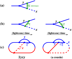
Figure 16: (a) An ordinary Feynman diagram represent a one-loop vertex correction to single splitting $g{\to}gg$, where we have highlighted the line $z=1{-}x{-}y$ in green. (b) The two time orderings in LCPT for the transverse-polarization contributions to that Feynman diagram. (c) Examples of rate diagrams that involve those time orderings of the amplitude. (Other examples just correspond to different choices of how to time-order the splitting in the conjugate amplitude relative to the interactions in the amplitude.) The first diagram in (c), $\bar{x}yxy$, is an example of a Class I virtual correction analyzed in ref. qcd . There, Class I diagrams must be added to their “cousins” obtained by swapping the two daughters of the splitting, $x\to 1{-}x$. The second diagram above is the cousin of the first, which can be seen by relabeling the loop variable $y$ in the second diagram by $y\to 1{-}y$. We haven’t relabeled $y$ here because that would destroy the correspondence of the label $z=1{-}x{-}y$ in (c) with the labeling of the original Feynman diagram in (a).

3.2.2 Practical considerations

Neither (47) nor (48) is convenient for numerical integration, especially since the detailed formula for ${\cal F}(x,y)$ is complicated enough to be mildly expensive to evaluate numerically. But now note that $\operatorname{PV}(1/z)$ is odd in $z{\to}-z$. Imagine that we changed the integration variables for $y$ to $z=1{-}x{-}y$ in (46a) to get an integral of the form

$$\int dz\>f(z)\,\operatorname{PV}\Bigl{[}\frac{1}{z}\Bigr{]},$$ (51)

where $f(z)$ is a continuous, non-singular function of $z$, corresponding to $z{\cal F}(x,y)$ in our case. If the bounds on integration over $z$ were symmetric about $z{=}0$, we would be able to average the integrand with $z\to-z$ to write

$$\int_{-a}^{a}dz\>f(z)\,\operatorname{PV}\Bigl{[}\frac{1}{z}\Bigr{]}=\int_{-a}^{a}dz\>\frac{f(z)-f(-z)}{2z}\,.$$ (52)

The integrand on the right-hand side is finite at $z{=}0$, and so it (i) no longer needs the PV prescription and (ii) is suitable for numerical integration. Unfortunately, our actual integration interval is not symmetric under $z{\to}-z$. We must divide the integration into different integration regions (one symmetric around $z{=}0$ and another that avoids $z{=}0$) and treat them differently. The shaded region of fig. 17 shows the largest region of $y$ that is symmetric under $y\to 2(1{-}x)-y$, which is the transformation that takes $z\to-{z}$ without changing $x$. Using (52) for the shaded region, the integral in (46a) can then be rewritten as the numerics-friendly expression

$$\left[\frac{d\Gamma}{dx}\right]_{\rm F,~{}virt~{}II}=2\operatorname{Re}\int_{0}^{1}dy\begin{cases}\tfrac{1}{2}\bigl{[}{\cal F}(x,y)+{\cal F}\bigl{(}x,2(1{-}x){-}y\bigr{)}\bigr{]};&1{-}2x\leq y\leq 2{-}2x,\\ {\cal F}(x,y)&\mbox{otherwise}.\end{cases}$$ (53)

Figure 17: The shading shows, for each value of $x$, the maximally-sized interval of $y$ integration that is symmetric under $(x,z)\to(x,-z)$, which translates to $y\to 2(1{-}x)-y$. The vertical dotted line is an example of the $y$ points for a particular value of $x$ and serves as a visual aid for the fact that, within the shaded region, the $y$ range with $z<0$ has the same size as the $y$ range with $z>0$.

4 Conclusion

A summary of formulas for the final results of this paper is given in appendix A. It is natural to wonder how much quantitative impact the processes of this paper (figs. 4–6) will have compared to the “nearly-complete” calculation of ref. qcd . With the tools presented so far, this is a somewhat ambiguous question. For example, virtual diagrams must be integrated over $y$. But the same integration of the virtual diagrams of ref. qcd gives an infrared divergence, which cannot be meaningfully compared to the non-divergent results of this paper. Even if one adds together the real and virtual diagrams of ref. qcd , there is still a double-log infrared divergence. A later paper finale will discuss how to make infrared-safe calculations of in-medium shower development, for which the relative size of contributions can then be examined. We leave that comparison until then.

Appendix A Summary

Appendix A of ref. qcd gave a summary, for the “nearly-complete” calculation there, of all rates associated with overlap effects in sequential gluon splitting. Here, we summarize how to add in the remaining diagrams analyzed in this paper.

A.1 $g\to ggg$ rate

Eq. (A.9) of ref. qcd for the total overlap effect on real double splitting should be modified to

$$\left[\Delta\frac{d\Gamma}{dx\,dy}\right]_{g{\to}ggg}=\left[\frac{d\Gamma}{dx\,dy}\right]_{\rm crossed}+\left[\Delta\frac{d\Gamma}{dx\,dy}\right]_{\rm seq}+\left[\frac{d\Gamma}{dx\,dy}\right]_{{\rm F}},$$ (54)

where the new term is

$$\left[\frac{d\Gamma}{dx\,dy}\right]_{{\rm F}}=\left[\frac{d\Gamma}{dx\,dy}\right]_{{\rm single~{}F}}+\left[\frac{d\Gamma}{dx\,dy}\right]_{({\rm FF})}.$$ (55)

A.1.1 single F piece

The “single F” piece corresponds to the analogous 4-gluon vertex result of section 4.1 of ref. 4point but with the substitution $\zeta_{(4)}\rightarrow\zeta_{\rm(F)}$ derived in this paper. That has the form

$$\left[\frac{d\Gamma}{dx\>dy}\right]_{{\rm single~{}F}}=\quad {\cal A}_{\rm(F)}(x,y)+{\cal A}_{\rm(F)}(1{-}x{-}y,y)+{\cal A}_{\rm(F)}(x,1{-}x{-}y)$$

$$+~{} {\cal A}_{\rm(F)}(y,x)+{\cal A}_{\rm(F)}(y,1{-}x{-}y)+{\cal A}_{\rm(F)}(1{-}x{-}y,x),$$ (56)

where ${\cal A}_{\rm(F)}(x,y)$ is the result of one color routing of $F\bar{y}\bar{x}+\bar{y}F\bar{x}+\bar{y}\bar{x}F$ (from fig. 4) plus conjugates. We’ll find it convenient later, for evaluating virtual diagrams, to split ${\cal A}_{\rm(F)}$ into separate contributions from each non-zero diagram (plus its conjugate):

$${\cal A}_{\rm(F)}(x,y)\equiv{\cal A}_{F\bar{y}\bar{x}}(x,y)+{\cal A}_{\bar{y}\bar{x}F}(x,y),$$ (57)

where

$${\cal A}_{F\bar{y}\bar{x}}(x,y) \equiv\int_{0}^{+\infty}d(\Delta t)\>2\operatorname{Re}\bigl{(}B_{F\bar{y}\bar{x}}(x,y,\Delta t)\bigr{)},$$ (58a)

$${\cal A}_{\bar{y}\bar{x}F}(x,y) \equiv\int_{0}^{+\infty}d(\Delta t)\>2\operatorname{Re}\bigl{(}B_{\bar{y}\bar{x}F}(x,y,\Delta t)\bigr{)},$$ (58b)

$$B_{F\bar{y}\bar{x}}(x,y,\Delta t) =D_{\rm(F)}(\hat{x}_{1},\hat{x}_{2},\hat{x}_{3},\hat{x}_{4},\zeta_{\rm(F)},\Delta t)=D_{\rm(F)}({-}1,y,1{-}x{-}y,x,\zeta_{\rm(F)},\Delta t),$$ (59a)

$$B_{\bar{y}\bar{x}F}(x,y,\Delta t) =D_{\rm(F)}(-\hat{x}_{4},-\hat{x}_{3},-\hat{x}_{2},-\hat{x}_{1},\zeta_{\rm(F)},\Delta t)=D_{\rm(F)}(-x,-(1{-}x{-}y),-y,1,\zeta_{\rm(F)},\Delta t),$$ (59b)

where $\zeta_{\rm(F)}\equiv\zeta_{\rm(F)}(x,y)$. Here, we follow the notation of Appendix A of ref. qcd by using hats over $(x_{1},x_{2},x_{3},x_{4})$ to represent our usual numbering convention (1):

$$(\hat{x}_{1},\hat{x}_{2},\hat{x}_{3},\hat{x}_{4})\equiv(-1,y,1{-}x{-}y,x).$$ (60)

Below, the $(x_{1},x_{2},x_{3},x_{4})$ without hats will instead generically represent whatever the arguments of the function $D$ are.

$$D_{\rm(F)}(x_{1}, x_{2},x_{3},x_{4},\zeta,\Delta t)=$$

$$-\frac{C_{\rm A}^{2}\alpha_{\rm s}^{2}M_{\rm f}}{16\pi^{2}E}\,(-x_{1}x_{2}x_{3}x_{4})\,\zeta\,\Omega_{+}\Omega_{-}\csc(\Omega_{+}\,\Delta t)\csc(\Omega_{-}\,\Delta t)\frac{Y_{\bar{\rm y}}}{X_{\bar{\rm y}}}\,,$$ (61)

where the low-level expressions for the symbols $M_{\rm f}$, $\Omega_{\pm}$, $X_{\bar{\rm y}}$ and $Y_{\bar{\rm y}}$ in terms of the arguments $(x_{1},x_{2},x_{3},x_{4},\Delta t)$ are the same as in appendices A.2.1 and A.2.2 of ref. qcd .

In (59), the argument $\zeta_{\rm(F)}$ passed to $D_{\rm(F)}$ is

$$\zeta_{\rm(F)}=\zeta_{(4)}+i_{12}\,\zeta_{12}-i_{14}\,\zeta_{14},$$ (62)

where

$$\zeta_{12}=\frac{(x^{2}{+}z^{2})(1{+}y^{2})}{(xyz)^{2}(1{-}y)^{3}}\,,\qquad\zeta_{13}=\frac{(1{-}y)^{4}+z^{2}+x^{2}y^{2}}{(xyz)^{2}(1{-}y)^{3}}\,,\qquad\zeta_{14}=\frac{(1{-}y)^{4}+x^{2}+z^{2}y^{2}}{(xyz)^{2}(1{-}y)^{3}}\,,$$ (63a)

$$\zeta_{(4)}=\zeta_{12}-2\zeta_{13}+\zeta_{14},$$ (63b)

$$i_{12}=\frac{(1{+}y)(x{-}z)}{(1{-}y)^{2}}\,,\qquad i_{14}=\frac{(1{+}x)(z{-}y)}{(1{-}x)^{2}}\,.$$ (63c)

A.1.2 FF piece

The FF piece corresponds to the $F\bar{F}$ diagram of fig. 4 plus its complex conjugate (which corresponds to the other time ordering, $\bar{F}F$). For the canonical color routing, the FF piece is given by (i) the 4-gluon vertex result for ${\cal A}_{(44)}$ in section 4.2 of ref. 4point times (ii) the factor indicated in our (40). The sum over color routings is then

$$\left[\frac{d\Gamma}{dx\>dy}\right]_{\rm(FF)}={\cal A}_{\rm(FF)}(x,y)+{\cal A}_{\rm(FF)}(1{-}x{-}y,y)+{\cal A}_{\rm(FF)}(x,1{-}x{-}y)$$ (64)

with

$${\cal A}_{\rm(FF)}(x,y)\equiv\bigl{[}1+\tfrac{1}{3}(i_{12}^{2}+i_{14}^{2}-i_{12}i_{14}+i_{12}-i_{14})\bigr{]}{\cal A}_{(44)}(x,y)$$ (65)

and

$${\cal A}_{(44)}(x,y)\equiv\int_{0}^{+\infty}d(\Delta t)\>2\operatorname{Re}\bigl{(}B_{(44)}(x,y,\Delta t)\bigr{)},$$ (66)

$$B_{(44)}(x,y,\Delta t) =C_{(44)}(\hat{x}_{1},\hat{x}_{2},\hat{x}_{3},\hat{x}_{4},\Delta t)=C_{(44)}({-}1,y,1{-}x{-}y,x,\Delta t),$$ (67)

$$C_{(44)}=D_{(44)}-\lim_{\hat{q}\to 0}D_{(44)},$$ (68)

$$D_{(44)}(x_{1},x_{2},x_{3},x_{4},\Delta t)=-\frac{3C_{\rm A}^{2}\alpha_{\rm s}^{2}}{16\pi^{2}}\,\Omega_{+}\Omega_{-}\csc(\Omega_{+}\,\Delta t)\csc(\Omega_{-}\,\Delta t).$$ (69)

A.2 NLO $g\to gg$ rate

The virtual corrections to single splitting $g{\to}gg$ are written in Appendix A.3 of ref. qcd in terms of

$$\left[\Delta\frac{d\Gamma}{dx}\right]^{\overline{\rm NLO}}_{g\to gg} =\biggl{(}\left[\Delta\frac{d\Gamma}{dx}\right]_{\rm virt\,I}\biggr{)}+(x\to 1{-}x)+\left[\Delta\frac{d\Gamma}{dx}\right]_{\rm virt\,II}$$

$$=\biggl{(}\int_{0}^{1-x}dy\,\left[\Delta\frac{d\Gamma}{dx\,dy}\right]_{\rm virt\,I}\biggr{)}+(x\to 1{-}x)+\int_{0}^{1}dy\,\left[\Delta\frac{d\Gamma}{dx\,dy}\right]_{\rm virt\,II},$$ (70)

where the three terms are, in order, the contribution of class I diagrams, their $x{\to}1{-}x$ cousins, and class II diagrams. Eqs. (A.53) and (A.54) of ref. qcd for the Class I and II $y$-integrands should be modified to

$$\left[\Delta\frac{d\Gamma}{dx\,dy}\right]_{\rm virt\,I}=\left[\frac{d\Gamma}{dx\,dy}\right]_{\rm virt\,Ic}+\left[\Delta\frac{d\Gamma}{dx\,dy}\right]_{\rm virt\,Is}+2\operatorname{Re}\left[\frac{d\Gamma}{dx\,dy}\right]_{xyy\bar{x}}+\left[\frac{d\Gamma}{dx\,dy}\right]_{\rm virt\,If}$$ (71)

and

$$\left[\Delta\frac{d\Gamma}{dx\,dy}\right]_{\rm virt\,II}=\left[\Delta\frac{d\Gamma}{dx\,dy}\right]_{\rm virt\,IIs}+2\operatorname{Re}\left[\frac{d\Gamma}{dx\,dy}\right]_{x\bar{y}\bar{y}\bar{x}}+\left[\frac{d\Gamma}{dx\,dy}\right]_{\rm virt\,IIf},$$ (72)

where the new addition is the last term in each.

A.2.1 $[d\Gamma/dx\,dy]_{\rm virt\,If}$

Given that $[d\Gamma/dx\,dy]_{\rm virt\,If}$ will be integrated over $0<y<1{-}x$ in (70), there are two equivalent ways to choose the integrand. One way is to include both color routings of the diagrams for every value of $y$ (the routings are related by $y\to 1{-}x{-}y$) and write the $y$-integrand in the form

$$\left[\frac{d\Gamma}{dx\,dy}\right]_{\rm virt\,If}=\tfrac{1}{2}\bigl{[}{\cal A}_{\rm virt\,If}(x,y)+{\cal A}_{\rm virt\,If}(x,1{-}x{-}y)\bigr{]},$$ (73a)

where $$\tfrac{1}{2} {\cal A}_{\rm virt\,If} y\leftrightarrow 1{-}x{-}y y$$ is the loop symmetry factor associated with the diagrams and is the result for a single color routing without including any loop symmetry factor. But, because of the symmetry of (73a), the integral is the same if we integrate only one color routing but drop the loop symmetry factor, and so instead take

$$\left[\frac{d\Gamma}{dx\,dy}\right]_{\rm virt\,If}={\cal A}_{\rm virt\,If}(x,y).$$ (73b)

Either way, (41) and (44) give

$${\cal A}_{\rm virt\,If}(x,y) =-{\cal A}_{F\bar{y}\bar{x}}(y,x)+\Bigl{[}{\cal A}_{F\bar{y}\bar{x}}(\tfrac{-x}{1-x-y},\tfrac{-y}{1-x-y})\Bigr{]}_{E\to(1-x-y)E}$$

$$=-{\cal A}_{F\bar{y}\bar{x}}(y,x)+(1{-}x{-}y)^{-1/2}{\cal A}_{F\bar{y}\bar{x}}(\tfrac{-x}{1-x-y},\tfrac{-y}{1-x-y}),$$ (74)

where the last line follows from the fact that rates $d\Gamma/dx\,dy$ are proportional to $\sqrt{\hat{q}_{\rm A}/E}$.

A.2.2 $[d\Gamma/dx\,dy]_{\rm virt\,IIf}$

Class II diagrams are integrated over $0<y<1$ in (70). Analogous to (73), we may write

$$\left[\frac{d\Gamma}{dx\,dy}\right]_{\rm virt\,IIf}=\tfrac{1}{2}\bigl{[}\,\overline{\cal A}_{\rm virt\,IIf}(x,y)+\overline{\cal A}_{\rm virt\,IIf}(x,1{-}y)\bigr{]}$$ (75a)

or

$$\left[\frac{d\Gamma}{dx\,dy}\right]_{\rm virt\,IIf}=\overline{\cal A}_{\rm virt\,IIf}(x,y).$$ (75b)

The latter is equivalent to the version presented in (46), with ${\cal A}_{\rm virt\,IIf}$ here representing $2\operatorname{Re}{\cal F}$. The overlines on ${\cal A}_{\rm virt\,IIf}$ in (75) will represent the averaging procedure of section 3.2.2. If we were instead content with $y$-integrands that had divergences requiring implementation of a principal value prescription, we could drop the overlines, and eqs. (42) and (43) give

$${\cal A}_{\rm virt\,IIf}(x,y)= =-\Bigl{[}{\cal A}_{\bar{y}\bar{x}F}(\tfrac{x}{1-y},\tfrac{-y}{1-y})\Bigr{]}_{E\to(1-y)E}+\Bigl{[}{\cal A}_{\bar{y}\bar{x}F}(\tfrac{y}{1-x},\tfrac{-x}{1-x})\Bigr{]}_{E\to(1-x)E}$$

$$=-(1{-}y)^{-1/2}{\cal A}_{\bar{y}\bar{x}F}(\tfrac{x}{1-y},\tfrac{-y}{1-y})+(1{-}x)^{-1/2}{\cal A}_{\bar{y}\bar{x}F}(\tfrac{y}{1-x},\tfrac{-x}{1-x}).$$ (76a)

Following (53), our numerics-friendly, averaged version $\overline{\cal A}_{\rm virt\,IIf}$ of ${\cal A}_{\rm virt\,IIf}$ is

$$\overline{\cal A}_{\rm virt\,IIf}(x,y)\equiv\begin{cases}\tfrac{1}{2}\bigl{[}{\cal A}_{\rm virt\,IIf}(x,y)+{\cal A}_{{\rm virt\,IIf}}\bigl{(}x,2(1{-}x){-}y\bigr{)}\bigr{]};&1{-}2x\leq y\leq 2{-}2x,\\ {\cal A}_{\rm virt\,IIf}(x,y)&\mbox{otherwise}.\end{cases}$$ (77)

References

- (1) L. D. Landau and I. Pomeranchuk, “Limits of applicability of the theory of bremsstrahlung electrons and pair production at high-energies,” Dokl. Akad. Nauk Ser. Fiz. 92 (1953) 535.
- (2) L. D. Landau and I. Pomeranchuk, “Electron cascade process at very high energies,” Dokl. Akad. Nauk Ser. Fiz. 92 (1953) 735.
- (3) A. B. Migdal, “Bremsstrahlung and pair production in condensed media at high-energies,” Phys. Rev. 103, 1811 (1956);
- (4) L. Landau, The Collected Papers of L.D. Landau (Pergamon Press, New York, 1965).
- (5) R. Baier, Y. L. Dokshitzer, A. H. Mueller, S. Peigne and D. Schiff, “The Landau-Pomeranchuk-Migdal effect in QED,” Nucl. Phys. B 478, 577 (1996) [arXiv:hep-ph/9604327];
- (6) R. Baier, Y. L. Dokshitzer, A. H. Mueller, S. Peigne and D. Schiff, “Radiative energy loss of high-energy quarks and gluons in a finite volume quark - gluon plasma,” Nucl. Phys. B 483, 291 (1997) [arXiv:hep-ph/9607355].
- (7) R. Baier, Y. L. Dokshitzer, A. H. Mueller, S. Peigne and D. Schiff, “Radiative energy loss and -broadening of high energy partons in nuclei,” ibid. 484 (1997) [arXiv:hep-ph/9608322].
- (8) B. G. Zakharov, “Fully quantum treatment of the Landau-Pomeranchuk-Migdal effect in QED and QCD,” JETP Lett. 63, 952 (1996) [arXiv:hep-ph/9607440].
- (9) B. G. Zakharov, “Radiative energy loss of high-energy quarks in finite size nuclear matter and quark-gluon plasma,” JETP Lett. 65, 615 (1997) [Pisma Zh. Eksp. Teor. Fiz. 63, 952 (1996)] [arXiv:hep-ph/9607440].
- (10) J. P. Blaizot and Y. Mehtar-Tani, “Renormalization of the jet-quenching parameter,” Nucl. Phys. A 929, 202 (2014) [arXiv:1403.2323 [hep-ph]].
- (11) E. Iancu, “The non-linear evolution of jet quenching,” JHEP 10, 95 (2014) [arXiv:1403.1996 [hep-ph]].
- (12) B. Wu, “Radiative energy loss and radiative -broadening of high-energy partons in QCD matter,” JHEP 12, 081 (2014) [arXiv:1408.5459 [hep-ph]].
- (13) P. Arnold and S. Iqbal, “The LPM effect in sequential bremsstrahlung,” JHEP 04, 070 (2015) [erratum JHEP 09, 072 (2016)] [arXiv:1501.04964 [hep-ph]].
- (14) P. Arnold, H. C. Chang and S. Iqbal, “The LPM effect in sequential bremsstrahlung 2: factorization,” JHEP 09, 078 (2016) [arXiv:1605.07624 [hep-ph]].
- (15) P. Arnold, H. C. Chang and S. Iqbal, “The LPM effect in sequential bremsstrahlung: dimensional regularization,” JHEP 10, 100 (2016) [arXiv:1606.08853 [hep-ph]].
- (16) P. Arnold, H. C. Chang and S. Iqbal, “The LPM effect in sequential bremsstrahlung: 4-gluon vertices,” JHEP 10, 124 (2016) [arXiv:1608.05718 [hep-ph]].
- (17) P. Arnold and S. Iqbal, “In-medium loop corrections and longitudinally polarized gauge bosons in high-energy showers,” JHEP 12, 120 (2018) [arXiv:1806.08796 [hep-ph]].
- (18) P. Arnold, S. Iqbal and T. Rase, “Strong- vs. weak-coupling pictures of jet quenching: a dry run using QED,” JHEP 05, 004 (2019) [arXiv:1810.06578 [hep-ph]].
- (19) P. Arnold, T. Gorda and S. Iqbal, “The LPM effect in sequential bremsstrahlung: nearly complete results for QCD,” JHEP 11, 053 (2020) [erratum JHEP 05, 114 (2022)] [arXiv:2007.15018 [hep-ph]].
- (20) G. P. Lepage and S. J. Brodsky, “Exclusive Processes in Perturbative Quantum Chromodynamics,” Phys. Rev. D 22, 2157 (1980).
- (21) S. J. Brodsky and G. P. Lepage, “Exclusive Processes in Quantum Chromodynamics” in Perturbative Quantum Chromodynamics, ed. A. H. Mueller, World Scientific (1989), pp. 93–240 [Adv. Ser. Direct. High Energy Phys. 5, 93 (1989)].
- (22) S. J. Brodsky, H. C. Pauli and S. S. Pinsky, “Quantum chromodynamics and other field theories on the light cone,” Phys. Rept. 301, 299 (1998) [hep-ph/9705477].
- (23) Y. V. Kovchegov and E. Levin, “Quantum chromodynamics at high energy,” Cambridge Monogr. Part. Phys. Nucl. Phys. Cosmol. 33 (2012); errata available, as of this writing, at https://www.asc.ohio-state.edu/kovchegov.1/typos.pdf or on the publisher’s web site under the book’s resources.
- (24) P. Arnold and O. Elgedawy, “The LPM Effect in sequential bremsstrahlung: corrections,” to appear in JHEP [arXiv:2202.04662 [hep-ph]].
- (25) P. Arnold, “Landau-Pomeranchuk-Migdal effect in sequential bremsstrahlung: From large- QCD to =3 via the SU() analog of Wigner 6- symbols,” Phys. Rev. D 100, no. 3, 034030 (2019) [arXiv:1904.04264 [hep-ph]].
- (26) P. Arnold, “Multi-particle potentials from light-like Wilson lines in quark-gluon plasmas: a generalized relation of in-medium splitting rates to jet-quenching parameters ,” Phys. Rev. D 99, no.5, 054017 (2019) [arXiv:1901.05475 [hep-ph]].
- (27) G. Leibbrandt, “Introduction to Noncovariant Gauges,” Rev. Mod. Phys. 59, 1067 (1987)
- (28) G. A. Chirilli, Y. V. Kovchegov and D. E. Wertepny, “Regularization of the Light-Cone Gauge Gluon Propagator Singularities Using Sub-Gauge Conditions,” JHEP 12, 138 (2015) [arXiv:1508.07962 [hep-ph]].
- (29) G. A. Chirilli, Y. V. Kovchegov and D. E. Wertepny, “Classical Gluon Production Amplitude for Nucleus-Nucleus Collisions: First Saturation Correction in the Projectile,” JHEP 03, 015 (2015) [arXiv:1501.03106 [hep-ph]].
- (30) W. M. Zhang and A. Harindranath, “Role of longitudinal boundary integrals in light front QCD,” Phys. Rev. D 48, 4868-4880 (1993) [arXiv:hep-th/9302119 [hep-th]].
- (31) P. Arnold, O. Elgedawy and S. Iqbal, in preparation.