Shortest Route to Non-Abelian Topological Order on a Quantum Processor

Abstract

A highly coveted goal is to realize emergent non-Abelian gauge theories and their anyonic excitations, which encode decoherence-free quantum information. While measurements in quantum devices provide new hope for scalably preparing such long-range entangled states, existing protocols using the experimentally established ingredients of a finite-depth circuit and a single round of measurement produce only Abelian states. Surprisingly, we show there exists a broad family of non-Abelian states—namely those with a Lagrangian subgroup—which can be created using these same minimal ingredients, bypassing the need for new resources such as feed-forward. To illustrate that this provides realistic protocols, we show how $D_{4}$ non-Abelian topological order can be realized, e.g., on Google’s quantum processors using a depth-11 circuit and a single layer of measurements. Our work opens the way towards the realization and manipulation of non-Abelian topological orders, and highlights counter-intuitive features of the complexity of non-Abelian phases.

The quantum statistics of particles is a foundational concept with far-reaching ramifications, and in two spatial dimensions, a remarkably rich set of ‘anyonic statistics’ arises Leinaas and Myrheim (1977); Wilczek (1982). Although not realized by fundamental particles, anyons emerge as effective quasi-particles in two-dimensional condensed matter systems, most notably the fractional Quantum Hall effect Halperin and Jain (2020). The most exotic extension of quantum statistics occurs with non-Abelian anyons Bais (1980); Moore and Seiberg (1989); Witten (1989); Kitaev (2003) which always come in degenerate quantum states (Fig. 1). Consequently, while braiding Abelian anyons only lead to a phase factor, braiding ‘non-Abelions’ leads to a matrix action on the degenerate states. This has evoked dreams of a physically fault-tolerant route to perform quantum computing, with quantum gates being executed by the motion of non-Abelian anyons Nayak et al. (2008). However, a key obstacle is finding states of matter hosting such non-Abelions, called non-Abelian topological order Wen (2004). The most compelling candidates so far are certain fractional quantum Hall states in the second Landau level ($\nu=5/2,\,12/5$) Moore and Read (1991); Halperin and Jain (2020); Nayak et al. (2008). However, non-Abelian states are more fragile compared compared to their Abelian counterparts Nayak et al. (2008); Dean et al. (2008) and the extreme conditions required to create quantum Hall states, combining high magnetic fields, pristine samples and millikelvin temperatures, all call for new approaches to creating such quantum states.

Meanwhile, the significant advances in near-term quantum devices Preskill (2018) open up the possibility of realizing non-Abelian states, not from cooling into the ground states, but from controlled quantum gates that entangle a product state to resemble ground states with non-Abelian excitations. Indeed, recent theory and experimental work has shown how certain Abelian states can be created in this way, in particular the toric code topological order Verresen et al. (2021a); Semeghini et al. (2021); Satzinger et al. (2021). However, the general strategy adopted in these works is essentially a form of adiabatic state preparation whose depth is required to scale with system size Bravyi et al. (2006), a formidable requirement when one wants to scale system size with limited depth quantum circuits.

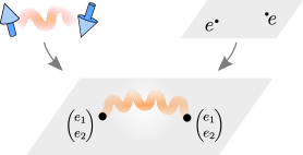
Figure 1: Artist’s impression of a non-Abelion. Non-Abelian anyons as in $D_{4}$ topological order bring together two ingredients in a remarkable mix: Bell pairs and gauge charges. Non-Abelions transform under a non-trivial matrix representation of the gauge group, leading to a topological degeneracy. The Bell pair is a robust consequence of forming a gauge neutral singlet. In this work we show how to efficiently prepare $D_{4}$ non-Abelian order with a single layer of measurement, whereby non-Abelion entanglement serves as a smoking gun.

Figure 2: Topological order from measurement. (a) By measuring the star term $A_{v}$ (1) of the toric code, $\mathbb{Z}_{2}$ topological order (TO) is obtained regardless of the measurement outcome. A clean toric code is achieved by pairing up $e$-anyons by a feed-forward of single-site Pauli operators. (b) In contrast, measuring non-Abelian gauge charges gives rise to topological degeneracies and non-Abelion entanglement (Fig. 1). Removing these requires a unitary circuit whose depth scales with system size Shi (2019). (c) One route to non-Abelian topological order is to first prepare two copies of the toric code by measuring the $e$-anyons in each layer. We obtain non-Abelian $D_{4}\cong\left(\mathbb{Z}_{2}\times\mathbb{Z}_{2}\right)\rtimes\mathbb{Z}_{2}$ topological order if we gauge the swap symmetry of the two layers. However, the Abelian anyon defects of the bilayer then become non-Abelian defects. (d) The aforementioned protocol does work if we use feed-forward to obtain two clean toric codes before gauging the swap symmetry. (e) In this work, we point out that one can obtain the same phase of matter without feed-forward, using only a single measurement layer. The key is to first prepare the two copies of the toric code by measuring the appropriate charges and fluxes which are invariant under the swap symmetry; subsequently gauging the swap symmetry does thus not introduce non-Abelian anyons. In fact, we can measure all three anyons at once. See Fig. 3 or Eq. (2) for an explicit and realistic circuit.

Remarkably, a workaround exists which allows to create certain topological orders in a time independent of system size. For instance, the aforementioned toric code is obtained at once by simply measuring its two commuting stabilizers on the links of the square lattice Gottesman (1997); Kitaev (2003); Raussendorf et al. (2005); Aguado et al. (2008); Piroli et al. (2021):

$$A_{v}=\raisebox{-20.0pt}{ \leavevmode\hbox to46.72pt{\vbox to46.72pt{\text{[drawing]}}} }\quad\textrm{and}\quad B_{p}=\raisebox{-20.0pt}{ \leavevmode\hbox to44.03pt{\vbox to40.06pt{\text{[drawing]}}} }. \sigma^{z} \sigma^{z} \sigma^{z} \sigma^{z} \sigma^{x} \sigma^{x} \sigma^{x} \sigma^{x} \sigma^{z} \sigma^{z} \sigma^{z} \sigma^{z} \sigma^{x} \sigma^{x} \sigma^{x} \sigma^{x}$$ (1)

Stronger yet, starting from a product state $\mathinner{|{\psi}\rangle}=\mathinner{|{+}\rangle}^{\otimes N}$, one needs to measure only $A_{v}$ (see Fig. 2a). The random measurement outcomes for $A_{v}$ do not affect the $\mathbb{Z}_{2}$ topological order: the resulting ‘$e$-anyons’ ($A_{v}=-1$) are static Abelian charges which simply redefine our notion of vacuum state. If one moreover wants to prepare the ‘clean’ case ($A_{v}=B_{p}=1$), we note that these $e$-anyons come in pairs and can be removed by a single feed-forward layer of $\sigma^{x}$-string operators Kitaev (2003).

The above approach generalizes to various other Abelian topological orders Bolt et al. (2016). However, the richer non-Abelian topological order does not admit such a simple stabilizer description, but at best only a commuting projector Hamiltonian Kitaev (2003); Levin and Wen (2005). Indeed, due to the intrinsic degeneracies associated to non-Abelions, the excited states do not resemble the ground state—in fact, they are not the ground state of any local gapped Hamiltonian. Hence, if one naively measures the terms in their parent Hamiltonian, one typically produces non-Abelian charges (Fig. 2b), which cannot even be paired up by any finite-depth unitary string operator Shi (2019). Intuitively, this is linked to the ‘Bell pair’ mentioned in Fig. 1.

This raises the question: is non-Abelian topological order out of the reach of a simple measurement protocol? Partial results are known where measurement helps: it has recently been shown that certain non-Abelian topological orders can be obtained in finite time by several layers of measurement, interspersed with feed-forward Verresen et al. (2021b); Tantivasadakarn et al. (2021); Bravyi et al. (2022); Lu et al. (2022). In light of these sophisticated protocols, and the aforementioned issue, it seems nigh impossible to obtain non-Abelian topological order from a single layer of measurements. This is of more than mere conceptual interest: feed-forward remains a very costly ingredient, with many quantum simulators and computing platforms not yet allowing for it. A protocol which avoids it, as for the toric code above, is thus of conceptual and practical significance.

Here, we show that a class of non-Abelian topological order can be created by a single layer of measurements, thereby thus not requiring feed-forward. Surprisingly, this shows that there exists a class of non-Abelian states which are no more complex to prepare than their Abelian counterparts, but nevertheless display richer behavior.

As a conceptually simple route towards non-Abelian order, let us imagine starting with two copies of the toric code. These can be prepared by measuring the star term $A_{v}$ (1) on each layer, producing $e_{1}$- and $e_{2}$-anyons on the two layers (Fig. 2c). Such a bilayer has a natural ‘swap’ symmetry interchanging the two copies. If this global physical symmetry were turned into a local gauge symmetry, we would achieve non-Abelian topological order. Indeed, the $e_{1}$ and $e_{2}$ anyons then transform as a doublet under the gauge group, which can be identified with $D_{4}=\left(\mathbb{Z}_{2}\times\mathbb{Z}_{2}\right)\rtimes\mathbb{Z}_{2}$ Barkeshli et al. (2019); SM . To obtain this gauge symmetry, we can proceed as in the toric code case, i.e., by simply measuring the gauge charge operator (or more precisely, its Gauss law operator); soon we make this more explicit. This has two effects: first, this produces a speckle of Abelian anyons associated to the swap gauge symmetry; this is as harmless as in the toric code case. A more serious issue is that the Abelian anyons of the toric code now turn into non-Abelian anyon defects (Fig. 2c).

Figure 3: Preparing non-Abelian $D_{4}$ topological order with a single layer of measurement: from theory to Sycamore chip. (a) The intuitive approach sketched in Fig. 2e is formalized in Eq. (2) for qubits on edges ($E$), vertices ($V$) and plaquettes ($P$) of the honeycomb lattice. Initializing all qubits in $\mathinner{|{+}\rangle}$, the circuit consists of three steps: 1) $CZ$ gates connecting plaquettes to vertices (dashed lines), which form the dice lattice. 2) $TH$ on the red vertices, and $T^{\dagger}H$ on the orange vertices (to wit, $T\propto e^{-i\frac{\pi}{8}Z}$). 3) $CZ$ gates connecting vertices to edges (solid lines), which forms the heavy-hex lattice. Finally, we measure all vertices and plaquettes in the $X$-basis, producing $D_{4}$ topological order for any measurement outcome, using only 9 layers of non-overlapping two-body gates. (b) Implementation on device with square lattice connectivity, e.g., Google’s Bristlecone and Sycamore chips. The first three panels prepare the dice lattice cluster state, the fourth panel performs the single-site basis rotation, and the last two panels applies the cluster state entangler for the heavy-hex lattice. Finally, measuring all but the purple-color qubits produces $D_{4}$ non-Abelian topological order. This protocol is independent of system size, requiring only 11 layers of non-overlapping two-body gates.

So far, the above example thus hits on the same stumbling block: in the quest to produce non-Abelian order via measurement, we produce defects which destroy the desired phase of matter. One possible solution is to clean up the $e$-anyon defects before gauging the swap symmetry (Fig. 2d); this gives a multi-step measurement protocol with feed-forward Verresen et al. (2021b); Tantivasadakarn et al. (2021); Bravyi et al. (2022); Lu et al. (2022) which—while interesting—we here seek to avoid. We surmise that this stumbling block cannot be avoided if one measures only charges. However, we show the issue can be resolved by using the larger freedom of measuring charges or fluxes (to wit, the fluxes of the toric code are also called $m$-anyons, as detected by $B_{p}$ in Eq. (1)). Indeed, rather than producing the toric code bilayer by measuring $e_{1}$ and $e_{2}$, we can also produce it by measuring a different set of Abelian anyons: the composites $e_{1}e_{2}$ and $m_{1}m_{2}$ (Fig. 2e). Crucially, these are a singlet under the swap symmetry. Hence, now proceeding as before, measuring the ‘swap anyons’ produces only Abelian defects. We have thereby produced $D_{4}$ topological order in finite time, without feed-forward! Observe that this approach works even if we measure the anyons $\{e_{1}e_{2},m_{1}m_{2},s\}$ all at once.

Let us now turn the above conceptual discussion into a concrete protocol for preparing $D_{4}$ topological order for qubits living on the edges ($E$) of the honeycomb lattice. To effectively measure the type of many-body operators discussed above, we will use two-body entangling gates and perform single-site measurements on ancilla qubits on the vertices ($V$) and plaquettes ($P$) of the honeycomb lattice. We claim that the topological order is obtained by the following sequence (Fig. 3a):

$$\mathinner{|{D_{4}}\rangle}_{E}=\mathinner{\langle{x}|}_{PV}\prod_{\langle v,e\rangle}CZ_{ve}\prod_{v}e^{\pm\frac{\pi i}{8}Z_{v}}H_{v}\;\prod_{\langle p,v\rangle}CZ_{pv}\mathinner{|{+}\rangle}_{PEV},$$ (2)

where $X,Y,Z$ denote Pauli matrices, $H$ is the Hadamard gate, $CZ$ is the Controlled-$Z$ gate, and $x=\pm 1$ denotes the arbitrary outcome upon measuring all the ancillas in the $X$-basis.

We can break the above procedure down into three steps. First, performing $CZ_{pv}$ prepares the dice lattice cluster state whereby measuring the plaquettes results in the color code. This is unitarily equivalent to two copies of the toric code Kubica et al. (2015), playing the role of the bilayer in Fig. 2e. The single-site gates on the vertices rotate the color code into a basis where the “swap” symmetry is realized by $\prod_{v}X_{v}$. Lastly, we gauge this symmetry by measuring its associated Gauss law operator on each vertex, $X_{v}\prod_{e\supset v}Z_{e}$, which is achieved by a single-site measurement preceded by the $CZ_{ve}$ unitary.

Importantly, any measurement in Eq. (2) can be delayed to the last step. A similar formula appeared in Ref. Verresen et al., 2021b, with the crucial difference that the single-site rotation was different. As a consequence, the latter requires feed-forward, corresponding to the scenario in Fig.2d.

Certain quantum processors have restricted connectivity, and might thus not be able to directly apply the gates in Fig.3a. In such cases it is still possible to create the $D_{4}$ state by using SWAP gates to attain the desired connectivity. To illustrate this, we propose an implementation for Google’s quantum processor, which has the connectivity of a square lattice as shown in Fig.3b. We find that the non-Abelian state can be prepared with a two-body depth of 11 layers, independent of total chip size. (This becomes 13 layers once we decompose the SWAP layers into Google’s native $CZ$ gates; see the Supplemental Materials SM for further discussion.)

While we have discussed the minimal case of $D_{4}$ topological order in great detail, we note that the idea of our efficient protocol extends to other topological orders which admit a so-called Lagrangian subgroup Kapustin and Saulina (2011); Levin (2013). This is defined to be a subgroup of Abelian anyons with trivial self and mutual statistics such that every other anyon in the theory braids non-trivially with it. In the case of $D_{4}$, this corresponds to the group generated by $\{e_{1}e_{2},m_{1}m_{2},s\}$ as encountered in Fig. 2e. Phrased in the language of quantum doubles Kitaev (2003), $e_{1}e_{2}$ and $s$ correspond to the sign representations of $D_{4}$, while $m_{1}m_{2}$ corresponds to the conjugacy class of the center of $D_{4}$ Barkeshli et al. (2019); SM . It is known that if one condenses the anyons in the Lagrangian subgroup, one obtains a trivial state. By playing this argument in reverse, one can argue that measuring the Gauss law operators associated to these anyons, one obtains its non-Abelian topological order with only a single layer of measurement SM . Other examples which can in principle be obtained in this way are, say, the quaternion $Q_{8}$ quantum doubleSM , or even the doubled Ising topological order Kitaev (2006); Levin and Wen (2005) (by measuring the Gauss law for $\epsilon$ and $\bar{\epsilon}$, though this requires physical fermions). It would be interesting to work out explicit protocols amenable to quantum processors, as we did for $D_{4}$ above.

In conclusion, we have established the simplest route to non-Abelian topological order. While the preparation time for a purely unitary protocol must scale with system size, we found that the minimal non-unitary element of a single measurement layer could efficiently prepare certain non-Abelian orders. This furthermore avoids the need for feed-forward which is intrinsic to multi-measurement approaches Verresen et al. (2021b); Tantivasadakarn et al. (2021); Bravyi et al. (2022); Lu et al. (2022). For the illustrative case of $D_{4}$, we found that roughly ten unitary layers (prior to single-site measurements) were already sufficient, even for realistic qubit connectivity as on the Google chips. Naturally, it would be worthwhile to work out concrete protocols for other existing architectures. On the conceptual side, the existence of a single-shot protocol for certain non-Abelian states motivates us to identify the minimal number of measurement layers (alongside finite-depth unitaries) for obtaining various types of quantum states. We will examine this measurement-induced hierarchy of quantum states in a forthcoming work Tantivasadakarn et al. (2023).

Lastly, if a non-Abelian state is realized, how do we tell? One interesting probe is the aforementioned non-Abelion entanglement (Fig. 1), which we can now turn into an advantage. Indeed, the successful preparation of non-Abelian order can be confirmed by noting that if we insert non-Abelian excitations, the entanglement entropy is changed according to its quantum dimension Kitaev and Preskill (2006). For instance, for our particular $D_{4}$ protocol (Eq. (2)), this is achieved by acting with Pauli-$Z$ operators on the vertices at any point prior to the single-site rotations. That such a deceptively simple tweak can have such a drastic consequence underlines the exotic nature of non-Abelian states, and points the way to the first realization and detection in a quantum simulator.

oneΔ

Appendix A Group theory of $D_{4}$

Figure 4: $D_{4}$ realizes the symmetries of the square. As a semidirect product $(\mathbb{Z}_{2}\times\mathbb{Z}_{2})\rtimes\mathbb{Z}_{2}$, the vertical and horizontal reflections ($rs$ and $r^{3}s$) are exchanged under the diagonal reflection $s$.

The group $D_{4}$ can be defined abstractly as generated by elements $r$ and $s$ which satisfy $r^{4}=s^{2}=(sr)^{2}=1$. As symmetries of the square, $r$ rotates the square by $90^{\circ}$ degrees and $s$ performs a diagonal reflection, as shown in Fig. 4. The group $D_{4}$ can also be seen as a semidirect product $(\mathbb{Z}_{2}\times\mathbb{Z}_{2})\rtimes\mathbb{Z}_{2}$, where the vertical and horizontal reflections $rs$ and $r^{3}s$ are swapped under diagonal symmetry $s$.

The group admits five irreducible representations (irreps). Other than the trivial irrep $\bm{1}$ and the faithful two-dimensional irrep $\bm{2}$ where

$$r =\begin{pmatrix}i&0\\ 0&-i\end{pmatrix}\qquad\textrm{and}\qquad s=\begin{pmatrix}0&1\\ 1&0\end{pmatrix},$$ (3)

there are three sign representations, which we will label $\bm{s}_{1}$, $\bm{s}_{2}$ and $\bm{s}_{3}$. Each sign rep is uniquely defined by its “kernel”, the subgroup on which the sign rep acts trivially.

1. $\bm{s}_{1}$ has kernel $\{1,r,r^{2},r^{3}\}$ meaning it is represented by $s=rs=r^{2}=r^{3}s=-1$,

2. $\bm{s}_{2}$ has kernel $\{1,r^{2},s,r^{2}s\}$ meaning it is represented by $r=r^{3}=rs=r^{3}s=-1$,

3. $\bm{s}_{3}$ has kernel $\{1,r^{2},rs,r^{3}s\}$ meaning it is represented by $r=r^{3}=s=r^{2}s=-1$.

The group also admits five conjugacy classes, $[1]=\{1\}$, $[r^{2}]=\{r^{2}\}$, $[r]=\{r,\bar{r}\}$, $[s]=\{s,\bar{r}^{2}s\}$ $[rs]=\{rs,r^{3}s\}$.

Appendix B Correspondence between anyons of bilayer Toric Code and anyons of $D_{4}$ TO

Mathematically, the anyons in the $G$ topological order (TO) corresponds to irreducible representations of the quantum double $\mathcal{D}(G)$. Each anyon can be given two labels: a conjugacy class $[g]$ and an irreducible representation of its centralizer $\pi_{g}$. A pure charge corresponds to the trivial conjugacy class with a choice of an irrep of $G$, while a pure flux corresponds a trivial irrep and a choice of conjugacy class. The quantum dimension of the anyon is given by the size of the conjugacy class times the dimension of the irrep. For $G=D_{4}$ enumerating all the possible choice of conjugacy classes and irreps gives a total of 22 anyons.

We are particularly interested in abelian anyons of $\mathcal{D}(D_{4})$ and how they are related to the anyons that we measure in the toric code bilayer construction: $e_{1}e_{2}$, $m_{1}m_{2}$, and $s$. A complete treatment of how anyons map under gauging (which is implemented in this particular instance by measurement) can be found in Ref. Barkeshli et al., 2019.

First, without loss of generality we take the swap symmetry to be represented by the group element $s$. As shown in Fig. 4 it exchanges $rs$ and $r^{3}s$, the vertical and horizontal reflections. Since $rs$ and $r^{3}s$ generate a $\mathbb{Z}_{2}\times\mathbb{Z}_{2}$ subgroup, which is the kernel of $\bm{s}_{3}$, we identify the gauge charge of the swap symmetry with $\bm{s}_{3}$ as a gauge charge of the $D_{4}$ quantum double.

Next, we note that $e_{1}e_{2}$ is a gauge charge of the bilayer toric code. In particular, it should be an irrep of the group $\mathbb{Z}_{2}\times\mathbb{Z}_{2}$. In $D_{4}$, this is the subgroup generated by $rs$ and $r^{3}s$. Now, since $e_{1}e_{2}$ is the charged under the gauge transformation of both symmetries, while neutral under the diagonal symmetry $r^{2}$, it must therefore correspond to a representation where $rs=r^{3}s=-1$ while $r^{2}=1$. Moreover, $e_{1}e_{2}$ is neutral under the swap symmetry, meaning $s=1$. Comparing to the irreps of $D_{4}$, we therefore see that this matches the irrep $\bm{s}_{2}$. By a similar argument, we find that $e_{1}e_{2}s$ corresponds to the irrep $\bm{s}_{1}$.

Finally, since $m_{1}m_{2}$ is a gauge flux of the bilayer toric code, it corresponds to a conjugacy class of $\mathbb{Z}_{2}\times\mathbb{Z}_{2}$. Since $m_{1}$ and $m_{2}$ are associated to group elements $rs$ and $r^{3}s$, their product is therefore $r^{2}$. Hence, $m_{1}m_{2}$ corresponds to the $r^{2}$ conjugacy class of $D_{4}$.

To conclude, the anyons we measure, $e_{1}e_{2},m_{1}m_{2},s$, generate eight anyons: $\{1,e_{1}e_{2},m_{1}m_{2},f_{1}f_{2},s,e_{1}e_{2}s,m_{1}m_{2}s,f_{1}f_{2}s\}$. It is apparent that these anyons are all bosons and have trivial mutual braiding. Therefore, after gauging they are identified with eight abelian anyons of $D_{4}$ that forms a $\mathbb{Z}_{2}^{3}$ Lagrangian subgroup. The exact correspondence is summarized in Table 1.

It is also worth pointing out how non-Abelian anyons are generated in this correspondence. First consider the anyon $e_{1}$, which corresponds to the irrep $(-1,1)$ of $\mathbb{Z}_{2}\times\mathbb{Z}_{2}$. Under the swap symmetry it transforms into $e_{2}$, corresponding to the irrep $(1,-1)$. Therefore, after gauging the swap symmetry, these two anyons combine into a single non-Abelian anyon with quantum dimension 2. This corresponds to the irrep $\bm{2}$ of $D_{4}$. Note that in this case, the non-trivial action on the anyons means that it is not meaningful to attach the charge of the swap symmetry onto $[e_{1}]$. Moreover, this can be interpreted as the fusion rule $\bm{2}\times\bm{s}_{3}=\bm{2}$ for $D_{4}$ anyons. Similarly, the anyon $m_{1}$ and $m_{2}$ corresponds to the conjugacy class $\{rs\}$ and $\{r^{3}s\}$ respectively. After gauging, the conjugation of $s$ combines them into a single conjugacy class $[rs]$ of $D_{4}$, resulting in a non-Abelian gauge flux.

For further details on this specific correspondence, we refer to a thorough review in Sec. II of Ref. Bulmash and Barkeshli, 2019.

Bilayer TC with SWAP symmetry ($\mathbb{Z}_{2}^{2}\rtimes\mathbb{Z}_{2}$)			$D_{4}$ Quantum Double			dim
Orbit of anyon under SWAP	Stabilizer	SWAP charge	Conj class	Centralizer	irrep
$[1]$	$\mathbb{Z}_{2}$	1	$[1]$	$D_{4}$	$\bm{1}$	1
$[e_{1}e_{2}]$	$\mathbb{Z}_{2}$	$s$	$[1]$	$D_{4}$	$\bm{s}_{1}$	1
$[e_{1}e_{2}]$	$\mathbb{Z}_{2}$	1	$[1]$	$D_{4}$	$\bm{s}_{2}$	1
$[1]$	$\mathbb{Z}_{2}$	$s$	$[1]$	$D_{4}$	$\bm{s}_{3}$	1
$[m_{1}m_{2}]$	$\mathbb{Z}_{2}$	1	$[{r^{2}}]$	$D_{4}$	$\bm{1}$	1
$[f_{1}f_{2}]$	$\mathbb{Z}_{2}$	$s$	$[{r^{2}}]$	$D_{4}$	$\bm{s}_{1}$	1
$[f_{1}f_{2}]$	$\mathbb{Z}_{2}$	1	$[{r^{2}}]$	$D_{4}$	$\bm{s}_{2}$	1
$[m_{1}m_{2}]$	$\mathbb{Z}_{2}$	$s$	$[{r^{2}}]$	$D_{4}$	$\bm{s}_{3}$	1
$[e_{1}]=\{e_{1},e_{2}\}$	$\mathbb{Z}_{1}$	1	$[1]$	$D_{4}$	$\bm{2}$	2
$[m_{1}]=\{m_{1},m_{2}\}$	$\mathbb{Z}_{1}$	1	$[rs]=\{rs,r^{3}s\}$	$\mathbb{Z}_{2}^{2}$	$\bm{1}$	2

Table 1: Correspondence between anyons of Bilayer TC along with the SWAP symmetry charge, and anyons of $D_{4}$ TO. (Certain anyons are omitted for simplicity.)

Appendix C Preparation of $D_{4}$ Topological order

Here we prove that the protocol in the main text indeed prepares the $D_{4}$ quantum double with a single round of measurement. We first define the protocol on the vertices edges and faces of the triangular lattice, where the preparation is most natural.

We place qubits on the vertices, edges and plaquettes of the triangular lattice as in Fig. 3a of the main text. For convenience, the protocol is reproduced here:

$$\mathinner{|{D_{4}}\rangle}_{E}=\mathinner{\langle{x}|}_{PV}\prod_{\langle v,e\rangle}CZ_{ve}\prod_{v}e^{\pm\frac{\pi i}{8}Z_{v}}H_{v}\;\prod_{\langle p,v\rangle}CZ_{pv}\mathinner{|{+}\rangle}_{PEV}.$$ (4)

Namely, we start with a product state $\mathinner{|{+}\rangle}$ for all qubits, apply the above quantum circuit, and perform projective measurements in the $x$-basis, where $x=\pm$ labels the measurement outcomes on each vertex and plaquette. Here, the $\pm$ sign in $e^{\pm\frac{\pi i}{8}Z_{v}}$ denotes that the phase gate we perform takes an alternating sign depending on the vertex sublattice (colored red or orange in in Fig. 3a of the main text).

The final state prepared, after a further Hadamard on all edges, is conveniently described as the simultaneous $+1$ eigenstate of the following “stabilizers”Yoshida (2016) defined for each vertex

$$\bm{A}_{p} ={\color[rgb]{1,0,0}{x_{p}}}\times\prod_{v\subset p}{\color[rgb]{0,0,1}x_{v}}\times\raisebox{-0.5pt}{\includegraphics[scale={0.9}]{ApD4.pdf}}, \bm{B}^{(1)}_{p} =\raisebox{-0.5pt}{\includegraphics[scale={0.9}]{Bp1D4.pdf}}, \bm{B}^{(2)}_{p} =\raisebox{-0.5pt}{\includegraphics[scale={0.9}]{Bp2D4.pdf}}.$$ (5)

as we will momentarily derive. Note that without the $CZ$ operators in $\bm{A}_{p}$, these describe the stabilizers of three copies of the toric code. The $CZ$ operators couple the toric code in a non-trivial way that creates the $D_{4}$ TO (see Appendix E.1 for a further relation to the $\mathbb{Z}_{2}^{3}$ twisted quantum double and SPT phases).

In this model, although $\bm{B}_{p}^{(i)}$ commutes with all operators, two adjacent $\bm{A}_{p}$ operators only commute up to some product of $\bm{B}_{p^{\prime}}^{(i)}$. For example, consider two adjacent plaquettes $p_{L}$ and $p_{R}$ sharing a vertical edge, then one has

$$\bm{A}_{p_{L}}\bm{A}_{p_{R}}=\bm{B}^{(1)}_{p_{L}}\bm{B}^{(2)}_{p_{R}}\bm{A}_{p_{R}}\bm{A}_{p_{L}}.$$ (6)

Nevertheless, one can still have a unique state which has eigenvalue $+1$ under all the above operators simultaneously, which is the state we prepare.

To facilitate in showing the above claim, we split the process into three steps

$$\mathinner{|{D_{4}}\rangle}_{E}=\mathinner{\langle{x}|}_{V}\prod_{\langle p,e\rangle}CZ_{pe}\mathinner{|{+}\rangle}_{E}\times e^{\pm\frac{\pi i}{8}Z_{v}}\prod_{v}H_{v}\times\mathinner{\langle{x}|}_{P}\prod_{\langle v,p\rangle}CZ_{vp}\mathinner{|{+}\rangle}_{PV}$$ (7)

The first step involves create a cluster state on the dice lattice by connecting each plaquette to each of the six vertices. Measuring all the plaquettes in the $x$-basis creates the color code. That is, the state

$$\mathinner{|{\text{CC}}\rangle}=\mathinner{\langle{x}|}_{P}\prod_{\langle v,p\rangle}CZ_{vp}\mathinner{|{+}\rangle}_{PV}$$ (8)

is the $+1$ eigenstate of the stabilizers

$$A_{p} ={\color[rgb]{0,0,1}{x_{p}}}\times\raisebox{-0.5pt}{\includegraphics[scale={0.9}]{ApCC.pdf}}, B_{p} =\raisebox{-0.5pt}{\includegraphics[scale={0.9}]{BpCC.pdf}}$$ (9)

For convenience, let us denote the six vertices surrounding the plaquettes as $1,\ldots,6$. Then,

$$A_{p} ={\color[rgb]{0,0,1}{x_{p}}}\times\prod_{n=1}^{6}Z_{n}, B_{p} =\prod_{n=1}^{6}X_{n} A_{p}B_{p}=-{\color[rgb]{0,0,1}{x_{p}}}\times\prod_{n=1}^{6}Y_{n}$$ (10)

Here, we have also included the product stabilizer to point out that the state inherently has a $\mathbb{Z}_{2}$ symmetry that swaps $A_{p}$ and $A_{p}B_{p}$ independent of the measurement outcome. This symmetry is realized by acting with $\frac{Y+Z}{\sqrt{2}}$ on one sublattice and $\frac{Y-Z}{\sqrt{2}}$ on the other sublattice. That is, on the six sites, it acts as $\prod_{n=1}^{6}\frac{Y+(-1)^{n}Z}{\sqrt{2}}$. (this sublattice structure is essential to obtain the minus sign in $A_{p}B_{p}$).

In order to measure the Gauss law for this symmetry, it is helpful to perform a basis transformation to turn the symmetry $\prod_{v}\frac{Y\pm Z}{\sqrt{2}}$ (where $\pm$ denotes the sublattice structure) into $\prod_{v}X_{v}$. This is accomplished by the second layer of the protocol: $\prod_{v}e^{\pm\frac{\pi i}{8}Z_{v}}H_{v}$ After the transformation, the state is given by stabilizers

$$\tilde{A}_{p} ={\color[rgb]{0,0,1}{x_{p}}}\times\prod_{n=1}^{6}\frac{X_{n}+(-1)^{n}Y_{n}}{\sqrt{2}} \tilde{B}_{p} =\prod_{n=1}^{6}Z_{n}, \tilde{A}_{p}\tilde{B}_{p}={\color[rgb]{0,0,1}{x_{p}}}\times\prod_{n=1}^{6}\frac{X_{n}-(-1)^{n}Y_{n}}{\sqrt{2}}.$$ (11)

Indeed, $\prod_{v}X_{v}$ swaps $\tilde{A}_{p}$ and $\tilde{A}_{p}\tilde{B}_{p}$ while leaving $\tilde{B}_{p}$ invariant as desired.

Finally, in the last step we measure the Gauss law for this $\mathbb{Z}_{2}$ symmetry $X_{v}\prod_{e\supset v}Z_{e}$ on all vertices.

This can be done by initializing qubits on all edges in the $\mathinner{|{+}\rangle}$ state, applying Controlled-$Z$ connecting vertices to all the nearest edges and measuring all the vertices in the X basis.

The new edges introduced are stabilized by $X_{e}$, and after applying $\prod_{v,e}CZ_{ve}$, the stabilizers are given by $\tilde{A}_{p}C_{p}$ and $\tilde{B}_{p}$ for each plaquette where

$$C_{p}=\raisebox{-0.5pt}{\includegraphics[scale={0.9}]{Cp.pdf}}$$ (12)

and $D_{e}=Z_{v}X_{e}Z_{v^{\prime}}$ for each edge, where $v$ and $v^{\prime}$ are the vertices at the end points of $e$. Now, to perform the measurement in the $X$ basis on all vertices, we need to find combinations of stabilizers that commute with the measurement. First, we note the following combinations do not involve vertex terms

$$B_{p}D_{12}D_{34}D_{56} =X_{12}X_{34}X_{56} B_{p}D_{23}D_{45}D_{61} =X_{23}X_{45}X_{61}.$$ (13)

and therefore survives the measurement. Next, we consider the symmetric combination

$$\tilde{A}_{p}C_{p}\frac{1+\tilde{B}_{p}}{2}={\color[rgb]{0,0,1}{x_{p}}}\times\prod_{n=1}^{6}X_{n}\times C_{p}\times\left[\prod_{n=1}^{6}\frac{1+(-1)^{n}iZ_{n}}{\sqrt{2}}+\prod_{n=1}^{6}\frac{1-(-1)^{n}iZ_{n}}{\sqrt{2}}\right]$$ (14)

Expanding the bracket we find

$$\tilde{A}_{p}C_{p}\frac{1+\tilde{B}_{p}}{2}={\color[rgb]{0,0,1}{x_{p}}}\times\prod_{n=1}^{6}X_{n}\times C_{p}\times\frac{1+\tilde{B}_{p}}{2}\prod_{n=1}^{6}\frac{1+Z_{n-1}Z_{n}+Z_{n}Z_{n+1}-Z_{n-1}Z_{n+1}}{2}$$ (15)

Since the state satisfies $\tilde{B}_{p}=1$, it therefore also has eigenvalue +1 under the “stabilizer”

$${\color[rgb]{0,0,1}{x_{p}}}\times\prod_{n=1}^{6}X_{n}\times C_{p}\times\prod_{n=1}^{6}\frac{1+Z_{n-1}Z_{n}+Z_{n}Z_{n+1}-Z_{n-1}Z_{n+1}}{2}$$ (16)

Note that these “stabilizers” no longer commute amongst themselves. Now, using the fact that the state satisfies $Z_{n}X_{n,n+1}Z_{n+1}=1$, we can replace $Z_{n}Z_{n+1}$ by$X_{n,n+1}$. This results in

$${\color[rgb]{0,0,1}{x_{p}}}\times\prod_{n=1}^{6}X_{n}\times C_{p}\times\prod_{n=1}^{6}\frac{1+X_{n-1,n}+X_{n,n+1}-X_{n-1,n}X_{n,n+1}}{2}$$ (17)

This “stabilizer” now commutes with the measurement on all vertices. With measurement outcomes $X_{n}={\color[rgb]{0,0,1}x_{n}}=\pm 1$. To conclude, the final “stabilizers” for each plaquette are

$${\color[rgb]{0,0,1}{x_{p}}}\times\prod_{n=1}^{6}{\color[rgb]{1,0,0}x_{n}}\times C_{p}\times\prod_{n=1}^{6}\frac{1+X_{n-1,n}+X_{n,n+1}-X_{n-1,n}X_{n,n+1}}{2}, X_{12}X_{34}X_{56}, X_{23}X_{45}X_{61}.$$ (18)

Finally, performing Hadamard on all edges and using the fact that $CZ_{ij}=\frac{1+Z_{i}+Z_{j}-Z_{i}Z_{j}}{2}$, we recover the “stabilizers” in Eq. (5).

Appendix D Implementation on Sycamore

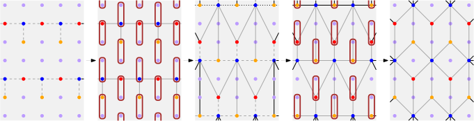
Figure 5: Preparation of the dice lattice cluster state in Sycamore using SWAP gates. Purple qubits only participate in the swapping procedure, and are not part of the cluster state.

First, let us count the depth of the 2-body gates required on the ideal lattice in Fig. 3a of the main text. The dice lattice cluster state can be prepared in depth 6, while the heavy-hex lattice cluster state can be prepared in depth 3. This gives a total 2-body depth count of 9.

Next, we discuss the details of implementation on the a quantum processor with connectivity of the square lattice, such as Google’s Sycamore quantum chip. The first step in our protocol $\prod_{\mathinner{\langle{p,v}\rangle}}CZ_{pv}$ requires preparing a cluster state on the dice lattice. This can be achieved by the help of SWAP gates. As seen in Fig. 5, the four steps corresponds to steps 1,2,3 and 5 in Fig. 3b, and indeed produces the cluster state.

Next, we note that the single site rotation $e^{\pm\frac{\pi i}{4}Z_{v}}H_{v}$ can be pulled back through the final layer of SWAP gates, so that it acts on the corresponding sites before the swap. This results in in step 4 of Fig. 3b. Lastly, $\prod_{\mathinner{\langle{v,e}\rangle}}CZ_{ve}$ which forms the heavy-hex lattice is implemented in step 6.

To count the number of gates used, the $CZ$ gates in steps 1 and 3 can each be implemented in depth-3. Therefore, the 2-body gate depth count for the six steps combined is is 3+1+3+0+1+3=11.

More practically, we should count the 2-body gate depth using the innate gates of the Sycamore processor. In particular, the SWAP gate can be decomposed in to three $CZ$ gates interspersed by Hadamard gates. Conveniently, one of the $CZ$ gates from the SWAP in step $5$ exactly cancels one of the $CZ$ layers in step 6. Thus, the innate 2-body depth count is 3+3+3+0+2+2=13.

Appendix E Single-round preparation of topological orders with Lagrangian subgroup

We give a formal argument that any non-Abelian topological order in two spatial dimensions which admits a Lagrangian subgroup can be prepared using a single round of measurements.

To recall, a Lagrangian subgroup $A$ is a subset of Abelian anyons that are closed under fusion, have trivial self and mutual statistics, and that every other anyon braids non-trivially with at least one of the anyons in the subgroupKapustin and Saulina (2011); Levin (2013). Note that the full set of anyons describing the theory does not need to be Abelian. Before moving forward, we remark that $A$ can serve two purposes in this discussion: it can be a set that contains anyons, or can also function as an abstract group.

Given a topological order and a Lagrangian subgroup $A$, one can “condense” Burnell (2018) all the anyons in $A$. To do this, we introduce an auxiliary system with global symmetry given by the group $A$. The system has charges that transform under irreps of the global symmetry $a_{\text{phys}}$. Note that these charges are physical, unlike the anyons $a$ which are gauge charges of an unphysical gauge group. Next, one performs a condensation for all bound states $a\times a_{\text{phys}}^{-1}$. This identifies $a\sim a_{\text{phys}}$ in the ground state of the condensed phase. The symmetry of the system is still $A$. However, the remaining anyons are confined, since they braid non-trivially with the anyons that are condensed. These confined anyons now serve as defects of the symmetry $A$. Since the resulting phase no longer has any anyons, it is therefore a (bosonic) Symmetry-Protected Topological (SPT) phase with global symmetry $A$. Let us call this state $\mathinner{|{\psi_{\text{SPT}}}\rangle}$ This process is also known as gauging the 1-form symmetry for all anyon lines in $A$Kapustin and Saulina (2011); Kaidi et al. (2022)

Now, we provide a protocol to prepare such a topological order. We start from a trivial product state with symmetry group $A$. It is known that any SPT phase in two spatial dimensions can be prepared (by temporarily breaking the symmetry) with a finite-depth local unitaryChen et al. (2013). Therefore, after preparing $\mathinner{|{\psi_{\text{SPT}}}\rangle}$, we measure the symmetry charges of $A$ by coupling the charges to ancillas so that we can measure its Gauss law. Note that this is nothing but the protocol to implement the Kramers-Wannier transformation in Ref. Tantivasadakarn et al., 2021. After the measurement, the charges of $\mathinner{|{\psi_{\text{SPT}}}\rangle}$ are promoted to gauge charges, and therefore realizes the anyons in $A$, and the symmetry fluxes are promoted to deconfined gauge fluxes, restoring the remaining anyons in the theory. In other words, our measurement has reversed the condensation by gauging the global symmetry $A$. To summarize, we have used finite-depth local unitaries and one round of measurement to prepare a state in the desired phase without feedforward or postselection. Note that if one moreover wants to prepare exactly the ground state of the phase, a single round of feedforward gates suffices to pair up all the anyons in $A$ that result from the measurement.

The condition of a Lagrangian subgroup can actually be relaxed if we allow physical fermions as resources. In particular, the subgroup $A^{f}$ can now contain anyons that have fermionic self-statistics, a fermionic Lagrangian algebraBultinck (2020). In this case, one performs “fermion condensation”Aasen et al. (2019). For any fermionic anyon in $A^{f}$ the bound state that one condenses is now $f\times f_{\text{phys}}^{-1}$. This gives a fermionic SPT state $\mathinner{|{\psi^{f}_{\text{SPT}}}\rangle}$ with global symmetry $A^{f}$, which contains fermion parity as a subgroup.

Similarly, starting with a trivial product state with fermionic symmetry $A^{f}$ it is possible to prepare the SRE state $\mathinner{|{\psi^{f}_{\text{SPT}}}\rangle}$ using finite-depth local unitaries. Then, one measures the Gauss law for this symmetry. For group elements that corresponds to anyons with fermionic statistics, measuring the Gauss law of the fermion amounts to performing the two-dimensional Jordan-Wigner transformation (bosonization)Chen et al. (2018), which can be performed using measurementsTantivasadakarn et al. (2021).

E.1 Example: $D_{4}$ TO revisited

To give a concrete example, let us consider the quantum double for $D_{4}$. The Lagrangian subgroup is given by the sign representations along with the conjugacy class of the center. These anyons form a group $A=\mathbb{Z}_{2}^{3}$. By performing condensation, one arrives at an invertible state with symmetry $\mathbb{Z}_{2}^{3}$. In fact, this state is a Symmetry-Protected Topological state, and can be deformed (while preserving the symmetry) to following hypergraph state Yoshida (2016)

$$\mathinner{|{\psi_{\text{SPT}}^{D_{4}}}\rangle}=\prod_{\langle p_{1}p_{2}p_{3}\rangle}CCZ_{p_{1}p_{2}p_{3}}\mathinner{|{+}\rangle}_{P}$$ (19)

where $\langle p_{1}p_{2}p_{3}\rangle$ denotes three plaquettes that share a common vertex. To describe the $\mathbb{Z}_{2}^{3}$ symmetry, we first note the plaquettes are three-colorable (say, red green and blue), such that no two adjacent plaquettes have the same color. Then each $\mathbb{Z}_{2}$ symmetry acts as spin flips on a plaquette of a fixed color.

To prepare the $D_{4}$ TO, we thus first prepare the above hypergraph state using $CCZ$. Then, we gauge the $\mathbb{Z}_{2}^{3}$ symmetry by measuring the Gauss law $\displaystyle X_{p}\prod_{e\in\raisebox{-0.4pt}{ \includegraphics[scale={0.25}]{eforZ23.pdf}}}Z_{e}$, where $e$ are the six edges radiating out of each plaquette. This can be done via

$$\mathinner{|{D_{4}}\rangle}_{E}=\mathinner{\langle{+}|}_{P}\prod_{p,e\in\raisebox{-0.4pt}{ \includegraphics[scale={0.25}]{eforZ23.pdf}}}CZ_{pe}\mathinner{|{+}\rangle}_{E}\mathinner{|{\psi_{\text{SPT}}^{D_{4}}}\rangle}$$ (20)

It is shown in Ref. Yoshida, 2016 that the resulting state (after applying Hadamard on all edges) has exactly the same “stabilizers” we derived in Eq. (5). This corresponds to the fact that the $D_{4}$ TO can be regarded as a $\mathbb{Z}_{2}^{3}$ twisted quantum doubleDijkgraaf et al. (1991); de Wild Propitius (1995); Hu et al. (2013).

E.2 Example: $Q_{8}$ TO

As a second example, we consider the quantum double for the quaternion group $Q_{8}$. The Lagrangian subgroup also consists of sign representations along with the conjugacy class of the center, and forms the group $A=\mathbb{Z}_{2}^{3}$. After condensation, we arrive at a different SPT state, corresponding to the following hypergraph state

$$\mathinner{|{\psi_{\text{SPT}}^{Q_{8}}}\rangle}=\prod_{\langle p_{1}^{C}p_{2}^{C}p_{3}^{C}\rangle}CCZ_{p_{1}^{C}p_{2}^{C}p_{3}^{C}}\prod_{\langle p_{1}p_{2}p_{3}\rangle}CCZ_{p_{1}p_{2}p_{3}}\mathinner{|{+}\rangle}_{P}$$ (21)

where $\langle p_{1}^{C}p_{2}^{C}p_{3}^{C}\rangle$ consists of three plaquettes of the same color connected by edges in a triangle shape.

Thus, the $Q_{8}$ TO can be prepared as

$$\mathinner{|{Q_{8}}\rangle}_{E}=\mathinner{\langle{+}|}_{P}\prod_{p,e\in\raisebox{-0.4pt}{ \includegraphics[scale={0.25}]{eforZ23.pdf}}}CZ_{pe}\mathinner{|{+}\rangle}_{E}\mathinner{|{\psi_{\text{SPT}}^{Q_{8}}}\rangle}$$ (22)

and the “stabilizers” of this state after Hadamard is given by

$$\bm{A}_{p} =\raisebox{-0.5pt}{\includegraphics[scale={0.9}]{ApQ81.pdf}}\times\raisebox{-0.5pt}{\includegraphics[scale={0.9}]{ApQ82.pdf}}, \bm{B}^{(1)}_{p} =\raisebox{-0.5pt}{\includegraphics[scale={0.9}]{Bp1D4.pdf}}, \bm{B}^{(2)}_{p} =\raisebox{-0.5pt}{\includegraphics[scale={0.9}]{Bp2D4.pdf}}.$$ (23)

E.3 Example: Double Ising TO

As a final example, we discuss how to prepare the Doubled Ising TO, which is obtained by stacking the Ising TO consisting of anyons $\{1,\sigma,\epsilon\}$ with its time-reversed partner $\{1,\bar{\sigma},\bar{\epsilon}\}$. Since $\epsilon$ and $\bar{\epsilon}$ are fermions, a Lagrangian subgroup does not exist. Nevertheless, it does have a fermionic Lagrangian subgroup $A^{f}=\{1,\epsilon,\bar{\epsilon},\epsilon\bar{\epsilon}\}$. Condensing the fermionic Lagrangian subgroup results in an SPT state with $\mathbb{Z}_{2}\times\mathbb{Z}_{2}^{F}$ symmetry. The precise wavefunction of this SPT state can be found in Ref. Tarantino and Fidkowski, 2016, and since it is short-range entangled, it can be prepared with a finite-depth quantum circuit.