Fast, high-order numerical evaluation of volume potentials via polynomial density interpolation

Abstract

This article presents a high-order accurate numerical method for the evaluation of singular volume integral operators, with attention focused on operators associated with the Poisson and Helmholtz equations in two dimensions. Following the ideas of the density interpolation method for boundary integral operators, the proposed methodology leverages Green’s third identity and a local polynomial interpolant of the density function to recast the volume potential as a sum of single- and double-layer potentials and a volume integral with a regularized (bounded or smoother) integrand. The layer potentials can be accurately and efficiently evaluated everywhere in the plane by means of existing methods (e.g. the density interpolation method), while the regularized volume integral can be accurately evaluated by applying elementary quadrature rules. We describe the method both for domains meshed by mapped quadrilaterals and triangles, introducing for each case (i) well-conditioned methods for the production of certain requisite source polynomial interpolants and (ii) efficient translation formulae for polynomial particular solutions. Compared to straightforwardly computing corrections for every singular and nearly-singular volume target, the method significantly reduces the amount of required specialized quadrature by pushing all singular and near-singular corrections to near-singular layer-potential evaluations at target points in a small neighborhood of the domain boundary. Error estimates for the regularization and quadrature approximations are provided. The method is compatible with well-established fast algorithms, being both efficient not only in the online phase but also to set-up. Numerical examples demonstrate the high-order accuracy and efficiency of the proposed methodology; applications to inhomogeneous scattering are mentioned.

65R20, 65D32

1 Introduction

This paper considers the numerical evaluation of volume integral operators of the form

(1) $$\mathcal{V}_{k}[f](\boldsymbol{x})\coloneqq\int_{\Omega}G_{k}(\boldsymbol{x},\boldsymbol{y})f(\boldsymbol{y})\,\mathrm{d}\boldsymbol{y},\quad\boldsymbol{x}\in\mathbb{R}^{2},$$

over bounded domains $\Omega\subset\mathbb{R}^{2}$ with piecewise-smooth boundary $\Gamma$, where $f\in C^{m}(\overline{\Omega})$, $m\geq 0$, is a given function (termed the source density), and where the operator kernel $G_{k}$ is the free-space Green’s function

(2) $$G_{k}(\boldsymbol{x},\boldsymbol{y})\coloneqq\begin{cases}\displaystyle-\frac{1}{2\pi}\log\left|\boldsymbol{x}-\boldsymbol{y}\right|,&k=0,\vskip 6.0pt plus 2.0pt minus 2.0pt\\ \displaystyle\frac{i}{4}H_{0}^{(1)}\left(k\left|\boldsymbol{x}-\boldsymbol{y}\right|\right),&k\neq 0,\end{cases}$$

for the Laplace ($k=0$) or Helmholtz ($k\neq 0$) equation. In fact, the method we propose is considerably more general than the examples presented, extending to (i) volume operators corresponding to these partial differential operators that possess stronger singularities such as the gradient of $\mathcal{V}_{k}$ as appears e.g. in [38],

(3) $$\mathcal{W}_{k}[\mathbf{f}](\boldsymbol{x})\coloneqq\int_{\Omega}\nabla_{\boldsymbol{y}}G_{k}(\boldsymbol{x},\boldsymbol{y})\cdot{\bf f}(\boldsymbol{y})\,\mathrm{d}\boldsymbol{y},\quad\boldsymbol{x}\in\mathbb{R}^{2},$$

where $\nabla_{\boldsymbol{y}}$ denotes a gradient with respect to the $\boldsymbol{y}$ variable, (ii) higher-dimensional analogues of these operators, and (iii) a variety of elliptic partial differential operators of interest in mathematical physics, e.g. in elasticity and fluids. Despite the broad utility of these operators, for example, to solve a nonlinear or an inhomogeneous linear PDE, until very recently the computation of volume potentials has been relatively neglected in the context of complex geometries; in what follows we outline some difficulties of this problem and present some alternatives to the volume potential.

There are several well-known challenges to be met for the efficient and accurate evaluation of operators such as Eq. 1 or Eq. 3 in complex geometries—some mirroring those of the more well-studied problem of layer potential evaluation and some unique to volume problems. As is well known, the free-space Green’s function $G_{k}$ given in Eq. 2 features a logarithmic singularity (whose location is, of course, dependent on the target evaluation point $\boldsymbol{x}$) that hinders the accuracy of standard quadrature rules for the numerical evaluation of the operator Eq. 1 or Eq. 3. Despite the requirement for some degree of local numerical treatment, the potential is a volumetric quantity depending globally on the source density, and as such it is especially important to couple its computation to global fast algorithms—of which a variety has been developed including $\mathcal{H}$-matrix compression and their directional counterparts [8, 9], the fast multipole method (FMM) [30], and, more recently, interpolated-factored Green function methods [7]. Generally, it is also desirable to construct numerical discretizations of the operators which are efficient for repeated application (e.g. in schemes involving iterative linear solvers, Newton-type iterations for nonlinearities, or time-stepping) or with values that can be efficiently accessed (e.g. for the construction of direct solvers).

The prototypical, but by no means exclusive, use case for volume operators of the form Eq. 1 is to tackle the slightly more specialized problem of producing a particular solution to an inhomogeneous constant-coefficient elliptic PDE. Restricting attention to work in this vein, where the resulting homogeneous problem is solved with integral equation techniques, there have been a variety of methods proposed for producing a valid particular solution, typically on uniform grids using finite difference, finite element, or Fourier methods—see [3] for more details. With the proviso that methods based on finite elements or finite differences are often of limited order of accuracy, they nonetheless do apply to piecewise-smooth domains. Fourier methods, in turn, relying on various concepts of Fourier extension to generate a highly-accurate Fourier series expansion of the density function (after which the production of a particular solution is straightforward) in particular have received significant attention as they allow the use of highly-efficient FFT algorithms. Such Fourier-based methods are either fundamentally limited to globally smooth domains [53, 52] or have only been demonstrated on such domains [22, 13]. Recently a scheme has been proposed [21] that allows extension on piecewise-smooth domains and, by coupling to highly-efficient volume Laplace FMMs [19] achieves an efficient and high-order accurate algorithm for producing a particular solution to Poisson’s equation. Another significant application of the volume operator Eq. 1 and Eq. 3 is in the numerical solution of Lippmann-Schwinger integral equations that arise in some formulations of inhomogeneous scattering problems; see e.g. [48, 56, 11, 1, 12].

The method proposed in this work directly evaluates the volume integral Eq. 1 using one of two meshing strategies for $\Omega$: (i) quadrilateral patch elements or (ii) a standard triangularization. Utilizing Green’s third identity, the value of the volume potential at each target point is related to a linear combination of regularized domain integrals, boundary integrals, and a local solution to the PDE that can be explicitly computed in terms of monomial sources. The method relies on local interpolants of the density function and explicit solutions to the underlying inhomogeneous PDE associated with those interpolated density functions.

Although the proposed approach is in spirit a natural extension of the density interpolation method [45, 46, 44, 26, 20], it shares several elements with previous methods. We first describe prior work in constructing local PDE solutions and then discuss the manner in which such solutions have historically been coupled to yield particular solutions valid on the entirety of the domain of interest. The first work we are aware of in which particular solutions were constructed using monomials is that of reference [4]; of course, the solutions are also polynomials. Subsequently, a variety of contributions studied combinations of polynomial sources and various elliptic partial differential operators; for monomials there exist solutions for Laplace [4], Helmholtz [25], and elasticity operators [39]. A particular solution formula that is applicable to second-order constant coefficient partial differential operators featuring a non-vanishing zeroth-order term and a monomial right-hand side was presented in [17]. Many of these methods can be considered to be closely related to the dual reciprocity method [41, 43]—such schemes rely on the density function being globally well-approximated by a collection of simple functions (e.g. polynomials, sinusoidal, or radial functions), and implicitly rely on the accurate and stable determination of coefficients in such expansions. This latter task has not generally been successfully executed to even moderate accuracy levels for complex geometries and/or density functions.

Thus, for an arbitrary complex geometry, in order to use the simple basis function expansions of the density function envisioned in reference [4] for a stable, high-order solver, one is naturally led to the use of subdivisions of the domain, wherein global solutions are stitched together from solutions defined with local data. The case of a rectangular domain that can be covered entirely by boxes is considered in reference [29] to construct a high-order Poisson solver. That work, similarly to the present method, uses local polynomial solutions (corresponding to Chebyshev polynomial right-hand sides) and layer potential corrections to provide a global solution. As described there, the local solution defined with data supported on a given element undergoes jumps across the boundary of that element, and it follows from Green’s identities that the particular solution, i.e. the volume potential, can be represented outside of the local element in terms of single- and double-layer potentials with polynomial densities defined explicitly in terms of the local element solution. This approach was also taken up using multi-wavelets on domains covered by a hierarchy of rectangular boxes in reference [6] as well as, in large part, in the three-dimensional works [32, 40].

We discuss next a few relevant distinctions between the present methodology and other more closely-related schemes. The scheme proposed in the present work differs from that introduced in reference [3] (see also [4]), where the volume potential is evaluated over irregular domain regions using a direct numerical quadrature of the singular and near-singular integrals. While the method presented in [3] requires only singular quadrature rules appropriate for the singular asymptotic behavior of the function $G_{k}$, its applicability may not include some of the more severely singular kernels which the present methodology and the density interpolation method naturally treat [26, 20]; additionally, the efficiency of that method suffers when gradients become large (e.g. $|k|$ large) with a wider near-field volume correction area needed. We turn next to methods that like ours leverage a polynomial solution to the underlying PDE and transform volume potentials to layer potentials. Unlike the previously-mentioned works [29, 6, 19, 32, 40] that rely on the method of images and/or pre-computed solutions for singular and near-singular evaluation points—since the grid and therefore the target locations have known structure in those settings—the present work applies to unstructured meshes wherein evaluation points may lay in arbitrary locations relative to element boundaries. Our method shares some elements with the work [51] that has contemporaneously appeared: both use Green’s third identity for volume potential evaluation over unstructured meshes, but, unlike that work, the class of near-singular layer potential evaluation schemes which we employ extends to three dimensions, treats operators with stronger singularities, and is, in principle, kernel-independent (see e.g. [20], though we stress that with regard to choice of methods for layer potential evaluation the scheme is agnostic).

An important feature of this method is that it results in a significant reduction in the number of singular corrections compared to previous volume potential schemes (even as the total number of volume corrections remains the same). This is made possible by the use of Green’s identity over a large region $\Gamma=\partial\Omega$ (illustrated in Figure 1) as opposed to element-wise boundaries, with the effect that, on the one hand, near-singular layer potential quadrature (e.g. with the density interpolation method) is only required in a thin region abutting $\Gamma$ while, on the other hand, volume quadrature for resulting regularized volume integrals provably can be effected to high-order accuracy with standard quadratures.

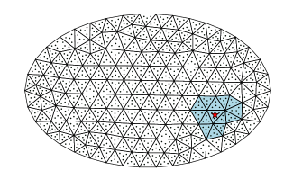
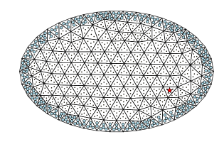
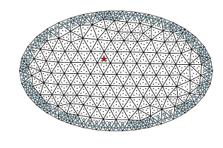
Figure 1: Comparison of the regions for which specialized quadrature is needed in two volume quadrature methods. Top: With the use of standard quadrature rules for $\mathcal{V}_{k}[f]$, nearby triangles for which the volume integral will be inaccurate for specific evaluation points collocated at a quadrature node and marked with a red star. Computation of the potential at all nodes displayed in the volume requires developing many (near-)singular quadrature rules for every triangle. Bottom: In the proposed methodology, in blue are marked the entirety of the volume evaluation points which lay close to the global domain boundary and at which points evaluation of layer potentials requires specialized quadratures—so as to evaluate the volume potential at all points in the domain (no specialized quadrature needed for evaluation points laying away from the boundary).

2 Preliminaries

In what follows we briefly outline the principles underlying the singular integration strategy employed in this paper. The method relies on polynomial approximations of the density function but is somewhat agnostic to the interpolation strategy. We present two specific strategies relying on one of

1. Taylor polynomials that match the function and its derivatives up to a certain order at a point $\boldsymbol{x}^{\star}\in\overline{\Omega}$, or

2. Lagrange interpolating polynomials over the entirety of an element $K$ in a triangulation.

Next, the method builds associated regularization polynomials that are particular solutions to the PDE with the interpolant as a right-hand side, and the interpolants and solutions are then used to regularize the volume integral in Eq. 1. Precisely, in case (i), we first explicitly construct a family of polynomial PDE solutions $\Phi_{n}(\cdot;\boldsymbol{x}^{\star}):\mathbb{R}^{2}\to\mathbb{C}$, the family being parametrized by $\boldsymbol{x}^{\star}\in\overline{\Omega}_{0}$, that satisfies

(4) $$(\Delta+k^{2})\Phi_{n}(\cdot;\boldsymbol{x}^{\star})=f_{n}(\cdot;\boldsymbol{x}^{\star})\quad\text{in}\quad\mathbb{R}^{2},$$

where $f_{n}(\cdot;\boldsymbol{x}^{\star}):\mathbb{R}^{2}\to\mathbb{C}$ is the polynomial of total degree $n$, also parametrized by $\boldsymbol{x}^{\star}$, that interpolates the density $f$ and its derivatives up to order $n$ at $\boldsymbol{x}^{\star}$; details about the construction of these polynomials are given in Section 3.1. Concerning the selection of $\boldsymbol{x}^{\star}$, we define

(5) $$\boldsymbol{x}^{\star}\coloneqq\operatorname*{argmin}_{\boldsymbol{y}\in\overline{\Omega}}|\boldsymbol{y}-\boldsymbol{x}|$$

and note that while our definition simplifies to $\boldsymbol{x}^{\star}=\boldsymbol{x}$ in the $\boldsymbol{x}\in\overline{\Omega}$ case on which we focus attention, the $\boldsymbol{x}\not\in\overline{\Omega}$ case is also of interest. In interpolation strategy (ii), on the other hand, over each triangle $K$ in a triangulation $\mathcal{T}_{h}$ of $\Omega$, we construct polynomials (now parametrized by the triangle $K$) $\Phi_{n}(\cdot;K):\mathbb{R}^{2}\to\mathbb{C}$, $K\in\mathcal{T}_{h}$, that satisfy

(6) $$(\Delta+k^{2})\Phi_{n}(\cdot;K)=f_{n}(\cdot;K)\quad\text{in}\quad\mathbb{R}^{2},$$

where $f_{n}(\cdot;K)$ is the polynomial of total degree $n$ that interpolates $f$ on a discrete set of points within the (possibly curvilinear) triangle $K$ which is closest to the target point $\boldsymbol{x}\in\mathbb{R}^{2}$ (typically, $\boldsymbol{x}\in K$); details about the construction of these polynomials, in turn, are given in Section 3.2.

Whichever the method by which a density interpolant and PDE-associated polynomial are generated, by next employing Green’s third identity and the solution $\Phi_{n}$ we arrive at the relation

(7) $$\mu(\boldsymbol{x})\Phi_{n}(\boldsymbol{x};\diamond)=-\int_{\Omega}G_{k}(\boldsymbol{x},\boldsymbol{y})f_{n}(\boldsymbol{y};\diamond)\,\mathrm{d}\boldsymbol{y}-\int_{\Gamma}\left\{\frac{\partial G_{k}(\boldsymbol{x},\boldsymbol{y})}{\partial n(\boldsymbol{y})}\Phi_{n}(\boldsymbol{y};\diamond)-G_{k}(\boldsymbol{x},\boldsymbol{y})\frac{\partial\Phi_{n}(\boldsymbol{y};\diamond)}{\partial n(\boldsymbol{y})}\right\}\,\mathrm{d}s(\boldsymbol{y}),$$

where

$$\mu(\boldsymbol{x})\coloneqq\begin{cases}1&\boldsymbol{x}\in\Omega,\\ \gamma(\boldsymbol{x})&\boldsymbol{x}\in\Gamma,\\ 0&\boldsymbol{x}\in\mathbb{R}^{2}\setminus\overline{\Omega},\end{cases}$$

with $\gamma(\boldsymbol{x})$ denoting a function proportional to the interior solid angle at $\boldsymbol{x}\in\Gamma$ that is equal to the familiar $\frac{1}{2}$ where $\Gamma$ is continuously differentiable [5, §8.1]. As usual, normal derivatives in (7) are taken with respect to the exterior unit normal to $\Gamma$. Here $\diamond$ is a placeholder for either $\boldsymbol{x}^{\star}$ in interpolation strategy (i) or $K$ in interpolation strategy (ii). From adding Eq. 7 to Eq. 1 it follows that the volume integral can be recast as

(8) $$\mathcal{V}_{k}[f](\boldsymbol{x})=\int_{\Omega}G_{k}(\boldsymbol{x},\boldsymbol{y})\{f(\boldsymbol{y})-f_{n}(\boldsymbol{y};\diamond)\}\,\mathrm{d}\boldsymbol{y}\\[-4.30554pt] -\int_{\Gamma}\left\{\frac{\partial G_{k}(\boldsymbol{x},\boldsymbol{y})}{\partial n(\boldsymbol{y})}\Phi_{n}(\boldsymbol{y};\diamond)-G_{k}(\boldsymbol{x},\boldsymbol{y})\frac{\partial\Phi_{n}(\boldsymbol{y};\diamond)}{\partial n(\boldsymbol{y})}\right\}\,\mathrm{d}s(\boldsymbol{y})-\mu(\boldsymbol{x})\Phi_{n}(\boldsymbol{x};\diamond).$$

In the sequel, we exploit Eq. 8 to develop an efficient, highly accurate method to numerically evaluate Eq. 1 everywhere in $\mathbb{R}^{2}$. Consider first the Taylor polynomial strategy (i): helpfully, since $f_{n}(\cdot;\boldsymbol{x}^{\star})$ is a Taylor interpolant of the density at $\boldsymbol{x}^{\star}$, the volume integrand in Eq. 8 is significantly smoother than the kernel $G_{k}$ itself and hence the regularized volume integral can be evaluated directly with high precision provided a suitable quadrature rule

(9) $$\mathcal{Q}_{\Omega}[\phi]\coloneqq\sum_{j=1}^{N}\omega_{j}\phi(\boldsymbol{\xi}_{j})\approx\int_{\Omega}\phi(\boldsymbol{y})\,\mathrm{d}\boldsymbol{y}$$

for smooth functions $\phi$ defined over $\Omega$ exists. On the other hand, considering now the Lagrange interpolation strategy (ii), $f-f_{n}(\cdot;\diamond)$ is small (in a sense made precise in Theorem 3.11) over the region near to $\boldsymbol{x}$ where $G_{k}$ is singular or experiences large gradients, and standard quadrature rules of the form Eq. 9 can again be utilized and yield high-order accuracy. The layer potentials in Eq. 8, on the other hand, can be accurately evaluated by means of existing techniques [26, 45, 44, 20]. For sufficiently regular trace functions $\varphi,\psi:\Gamma\to\mathbb{C}$, such techniques yield high-order approximations

$$\mathcal{B}_{\Gamma}[\varphi,\psi](\boldsymbol{x})\approx\int_{\Gamma}\left\{\frac{\partial G_{k}(\boldsymbol{x},\boldsymbol{y})}{\partial n(\boldsymbol{y})}\varphi(\boldsymbol{y})-G_{k}(\boldsymbol{x},\boldsymbol{y})\psi(\boldsymbol{y})\right\}\,\mathrm{d}s(\boldsymbol{y}),\quad\boldsymbol{x}\in\mathbb{R}^{2},$$

where $\mathcal{B}_{\Gamma}$ stands for (any) sufficiently accurate approximation of the boundary integrals.

In order to make the evaluation of Eq. 8 efficient, we avoid having to recompute all the integrals associated with the polynomial terms as the evaluation point $\boldsymbol{x}\in\mathbb{R}^{2}$ varies. We do so by expressing $f_{n}$ and $\Phi_{n}$ in terms of fixed monomials so that the application of the volume and layer potentials to the monomials can be precomputed and reused. Indeed, expanding the interpolant as

(10) $$f_{n}(\boldsymbol{y};\diamond)=\sum_{|\alpha|\leq n}c_{\alpha}[f](\diamond)p_{\alpha}(\boldsymbol{y}),\qquad p_{\alpha}(\boldsymbol{y})\coloneqq\frac{\boldsymbol{y}^{\alpha}}{\alpha!},$$

i.e. in a normalized monomial basis, we readily obtain that

(11) $$\Phi_{n}(\boldsymbol{y};\diamond)=\sum_{|\alpha|\leq n}c_{\alpha}[f](\diamond)P_{\alpha}(\boldsymbol{y}),$$

where the polynomials $\{P_{\alpha}\}_{|\alpha|\leq n}$, of total degree less than or equal to $n\in\mathbb{N}_{0}$, satisfy the inhomogeneous Laplace/Helmholtz equation:

(12) $$(\Delta+k^{2})P_{\alpha}=p_{\alpha}\quad\text{in}\quad\mathbb{R}^{2}.$$

Here and in what follows, we make use of the standard multi-index notation where, for any $\alpha=(\alpha_{1},\alpha_{2})\in\mathbb{N}_{0}^{2}$, we set $\alpha!=\alpha_{1}!\alpha_{2}!$, $|\alpha|=\alpha_{1}+\alpha_{2}$, $\boldsymbol{y}^{\alpha}=y_{1}^{\alpha_{1}}y_{2}^{\alpha_{2}}$ when $\boldsymbol{y}=(y_{1},y_{2})\in\mathbb{R}^{2}$, and

$${\binom{\alpha}{\beta}}=\frac{\alpha!}{(\alpha-\beta)!\beta!}=\frac{\alpha_{1}!}{(\alpha_{1}-\beta_{1})!\beta_{1}!}\frac{\alpha_{2}!}{(\alpha_{2}-\beta_{2})!\beta_{2}!}$$

when $\beta=(\beta_{1},\beta_{2})\in\mathbb{N}_{0}^{2}$. The construction of the polynomial PDE solutions $P_{\alpha}$ corresponding to the monomial sources $p_{\alpha}$ is based on the procedures presented in [2].

In the case of Taylor interpolation, the coefficients in Eq. 10 are obtained by employing the binomial theorem to translate the expansion point at $\boldsymbol{x}^{\star}$ in Eq. 18 to the origin. The same technique is utilized for Lagrange interpolation, but for a different purpose: in Lagrange interpolation it is useful to solve the multivariate Vandermonde system in coordinates local to the triangle, and the translation operators yield again the resulting global polynomials. In both approaches, the coefficients of the interpolation polynomial $\{c_{\alpha}[f](\diamond)\}_{|\alpha|\leq n}$ in Eq. 10 are computed using only the density values at the given set of quadrature nodes $\{\boldsymbol{\xi}_{j}\}_{j=1}^{N}$ in Eq. 9.

Leveraging the expansions Eq. 10 and Eq. 11, it then follows that $\mathcal{V}_{k}[f](\boldsymbol{x})$ for $\boldsymbol{x}\in\mathbb{R}^{2}$, can be approximated as

(13) $$\mathcal{V}_{k}[f](\boldsymbol{x})\approx\mathcal{Q}_{\Omega}\left[\mathchoice{\mathop{\vbox{\halign{#\cr\kern 0.80002pt$\hss\leavevmode\resizebox{6.29001pt}{3.8889pt}{\rotatebox[origin={c}]{90.0}{(}}\hss$\crcr\nointerlineskip\cr$\hss\displaystyle G\hss$\crcr}}}\limits}{\mathop{\vbox{\halign{#\cr\kern 0.80002pt$\hss\leavevmode\resizebox{6.29001pt}{3.8889pt}{\rotatebox[origin={c}]{90.0}{(}}\hss$\crcr\nointerlineskip\cr$\hss\textstyle G\hss$\crcr}}}\limits}{\mathop{\vbox{\halign{#\cr\kern 0.80002pt$\hss\leavevmode\resizebox{4.403pt}{2.72223pt}{\rotatebox[origin={c}]{90.0}{(}}\hss$\crcr\nointerlineskip\cr$\hss\scriptstyle G\hss$\crcr}}}\limits}{\mathop{\vbox{\halign{#\cr\kern 0.80002pt$\hss\leavevmode\resizebox{3.145pt}{1.94444pt}{\rotatebox[origin={c}]{90.0}{(}}\hss$\crcr\nointerlineskip\cr$\hss\scriptscriptstyle G\hss$\crcr}}}\limits}_{k}(\boldsymbol{x},\cdot)f(\cdot)\right]-\sum_{|\alpha|\leq n}c_{\alpha}[f](\diamond)\big{\{}\mathcal{Q}_{\Omega}\big{[}\mathchoice{\mathop{\vbox{\halign{#\cr\kern 0.80002pt$\hss\leavevmode\resizebox{6.29001pt}{3.8889pt}{\rotatebox[origin={c}]{90.0}{(}}\hss$\crcr\nointerlineskip\cr$\hss\displaystyle G\hss$\crcr}}}\limits}{\mathop{\vbox{\halign{#\cr\kern 0.80002pt$\hss\leavevmode\resizebox{6.29001pt}{3.8889pt}{\rotatebox[origin={c}]{90.0}{(}}\hss$\crcr\nointerlineskip\cr$\hss\textstyle G\hss$\crcr}}}\limits}{\mathop{\vbox{\halign{#\cr\kern 0.80002pt$\hss\leavevmode\resizebox{4.403pt}{2.72223pt}{\rotatebox[origin={c}]{90.0}{(}}\hss$\crcr\nointerlineskip\cr$\hss\scriptstyle G\hss$\crcr}}}\limits}{\mathop{\vbox{\halign{#\cr\kern 0.80002pt$\hss\leavevmode\resizebox{3.145pt}{1.94444pt}{\rotatebox[origin={c}]{90.0}{(}}\hss$\crcr\nointerlineskip\cr$\hss\scriptscriptstyle G\hss$\crcr}}}\limits}_{k}(\boldsymbol{x},\cdot)p_{\alpha}(\cdot)\big{]}+\mathcal{B}_{\Gamma}[P_{\alpha},\partial_{n}P_{\alpha}](\boldsymbol{x})+\mu(\boldsymbol{x})P_{\alpha}(\boldsymbol{x})\big{\}}$$

where we make use of the punctured Green’s functions

(14) $$\mathchoice{\mathop{\vbox{\halign{#\cr\kern 0.80002pt$\hss\leavevmode\resizebox{6.29001pt}{3.8889pt}{\rotatebox[origin={c}]{90.0}{(}}\hss$\crcr\nointerlineskip\cr$\hss\displaystyle G\hss$\crcr}}}\limits}{\mathop{\vbox{\halign{#\cr\kern 0.80002pt$\hss\leavevmode\resizebox{6.29001pt}{3.8889pt}{\rotatebox[origin={c}]{90.0}{(}}\hss$\crcr\nointerlineskip\cr$\hss\textstyle G\hss$\crcr}}}\limits}{\mathop{\vbox{\halign{#\cr\kern 0.80002pt$\hss\leavevmode\resizebox{4.403pt}{2.72223pt}{\rotatebox[origin={c}]{90.0}{(}}\hss$\crcr\nointerlineskip\cr$\hss\scriptstyle G\hss$\crcr}}}\limits}{\mathop{\vbox{\halign{#\cr\kern 0.80002pt$\hss\leavevmode\resizebox{3.145pt}{1.94444pt}{\rotatebox[origin={c}]{90.0}{(}}\hss$\crcr\nointerlineskip\cr$\hss\scriptscriptstyle G\hss$\crcr}}}\limits}_{k}(\boldsymbol{x},\boldsymbol{y})=\begin{cases}G_{k}(\boldsymbol{x},\boldsymbol{y}),&\boldsymbol{y}\neq\boldsymbol{x},\\ 0,&\boldsymbol{y}=\boldsymbol{x},\end{cases}\quad\text{or}\quad\mathchoice{\mathop{\vbox{\halign{#\cr\kern 0.80002pt$\hss\leavevmode\resizebox{6.29001pt}{3.8889pt}{\rotatebox[origin={c}]{90.0}{(}}\hss$\crcr\nointerlineskip\cr$\hss\displaystyle G\hss$\crcr}}}\limits}{\mathop{\vbox{\halign{#\cr\kern 0.80002pt$\hss\leavevmode\resizebox{6.29001pt}{3.8889pt}{\rotatebox[origin={c}]{90.0}{(}}\hss$\crcr\nointerlineskip\cr$\hss\textstyle G\hss$\crcr}}}\limits}{\mathop{\vbox{\halign{#\cr\kern 0.80002pt$\hss\leavevmode\resizebox{4.403pt}{2.72223pt}{\rotatebox[origin={c}]{90.0}{(}}\hss$\crcr\nointerlineskip\cr$\hss\scriptstyle G\hss$\crcr}}}\limits}{\mathop{\vbox{\halign{#\cr\kern 0.80002pt$\hss\leavevmode\resizebox{3.145pt}{1.94444pt}{\rotatebox[origin={c}]{90.0}{(}}\hss$\crcr\nointerlineskip\cr$\hss\scriptscriptstyle G\hss$\crcr}}}\limits}_{k}(\boldsymbol{x},\boldsymbol{y})=\begin{cases}G_{k}(\boldsymbol{x},\boldsymbol{y}),&\boldsymbol{y}\notin K\\ 0,&\boldsymbol{y}\in K,\end{cases}$$

depending on the interpolation strategy employed, (i) or (ii), respectively. As usual, the symbol $\partial_{n}$ in Eq. 13 denotes the derivative along the exterior unit normal to the boundary $\Gamma$, while in Eq. 14 $K$ denotes the element such that $\boldsymbol{x}\in K$.

The efficiency of the proposed methodology becomes evident from considering the evaluation of the approximation Eq. 13 to $\mathcal{V}_{k}[f]$ at all the $N$-numbered volume quadrature nodes $\{\boldsymbol{\xi}_{j}\}_{j=1}^{N}$ in the mesh. In either of the discretization strategies (i) or (ii), the interpolation polynomial $f_{n}$ is expanded in terms of the monomials $\{p_{\alpha}\}_{|\alpha|\leq n}$—a fixed monomial basis, of cardinality

(15) $$q_{n}\coloneqq(n+1)(n+2)/2,$$

on which the action of $\mathcal{Q}_{\Omega}$ is precomputed. Table 1 provides an overview of the computational costs associated with these evaluations, assuming that the FMM is utilized to accelerate the volume and boundary integral computations. (Clearly, the layer and volume potential pre-computations inherent in Eq. 13, i.e. the computations listed in the $f$-independent rows in Table 1, can be computed in an embarrassingly-parallel fashion across the polynomial degree multi-index $\alpha$.)

The costs in Table 1 for evaluating $\mathcal{Q}_{\Omega}[\mathchoice{\mathop{\vbox{\halign{#\cr\kern 0.80002pt$\hss\leavevmode\resizebox{6.29001pt}{3.8889pt}{\rotatebox[origin={c}]{90.0}{(}}\hss$\crcr\nointerlineskip\cr$\hss\displaystyle G\hss$\crcr}}}\limits}{\mathop{\vbox{\halign{#\cr\kern 0.80002pt$\hss\leavevmode\resizebox{6.29001pt}{3.8889pt}{\rotatebox[origin={c}]{90.0}{(}}\hss$\crcr\nointerlineskip\cr$\hss\textstyle G\hss$\crcr}}}\limits}{\mathop{\vbox{\halign{#\cr\kern 0.80002pt$\hss\leavevmode\resizebox{4.403pt}{2.72223pt}{\rotatebox[origin={c}]{90.0}{(}}\hss$\crcr\nointerlineskip\cr$\hss\scriptstyle G\hss$\crcr}}}\limits}{\mathop{\vbox{\halign{#\cr\kern 0.80002pt$\hss\leavevmode\resizebox{3.145pt}{1.94444pt}{\rotatebox[origin={c}]{90.0}{(}}\hss$\crcr\nointerlineskip\cr$\hss\scriptscriptstyle G\hss$\crcr}}}\limits}_{k}(\boldsymbol{\xi}_{j},\cdot)f(\cdot)]$, $\mathcal{Q}_{\Omega}\big{[}\mathchoice{\mathop{\vbox{\halign{#\cr\kern 0.80002pt$\hss\leavevmode\resizebox{6.29001pt}{3.8889pt}{\rotatebox[origin={c}]{90.0}{(}}\hss$\crcr\nointerlineskip\cr$\hss\displaystyle G\hss$\crcr}}}\limits}{\mathop{\vbox{\halign{#\cr\kern 0.80002pt$\hss\leavevmode\resizebox{6.29001pt}{3.8889pt}{\rotatebox[origin={c}]{90.0}{(}}\hss$\crcr\nointerlineskip\cr$\hss\textstyle G\hss$\crcr}}}\limits}{\mathop{\vbox{\halign{#\cr\kern 0.80002pt$\hss\leavevmode\resizebox{4.403pt}{2.72223pt}{\rotatebox[origin={c}]{90.0}{(}}\hss$\crcr\nointerlineskip\cr$\hss\scriptstyle G\hss$\crcr}}}\limits}{\mathop{\vbox{\halign{#\cr\kern 0.80002pt$\hss\leavevmode\resizebox{3.145pt}{1.94444pt}{\rotatebox[origin={c}]{90.0}{(}}\hss$\crcr\nointerlineskip\cr$\hss\scriptscriptstyle G\hss$\crcr}}}\limits}_{k}(\boldsymbol{\xi}_{j},\cdot)p_{\alpha}(\cdot)\big{]}$, and $\mathcal{B}_{\Gamma}[P_{\alpha},\partial_{n}P_{\alpha}](\boldsymbol{\xi}_{j})$ are the costs of FMM-accelerated summation at $\mathcal{O}(N)$ volume target points; the FMM-accelerated general-purpose DIM [20] is utilized to evaluate the boundary integrals $\mathcal{B}_{\Gamma}$, with the boundary discretized using $N_{b}\propto N^{1/2}$ points. Turning to coefficient $c_{\alpha}[f]$ evaluation, the cost of computing all $q_{n}$ derivatives in the Taylor series for method (i) is $\mathcal{O}(q_{n}N\log N)$ due to the use of FFT-based differentiation costing $\mathcal{O}(N\log N)$ per derivative (cf. Eq. 18 and Section 3.1.2), while the cost of performing the translation operations over all $N$ evaluation points in the mesh is clearly $\mathcal{O}(q_{n}^{2}N)$ in view of Eq. 26. In the Lagrange methodology (ii), on the other hand, a linear system of size $q_{n}$ must be factored for each of the $L$ elements, which amounts to a cost of $\mathcal{O}(q_{n}^{2}N)$, while the translation for each of the $L$ elements costs a total of $\mathcal{O}(q_{n}N)$. Overall, the operation count estimate shows that, for a given interpolation order $n\in\mathbb{N}_{0}$, the volume-DIM methodology achieves near-optimal complexity and is confirmed by the numerical results in Section 4.

In addition, the regularization of the operator $\mathcal{W}_{k}$ can be achieved in a similar manner by interpolating $\mathbf{f}$ component-wise. Indeed, letting $\mathbf{f}_{n}(\cdot;\diamond)$ denote the corresponding polynomial interpolant of the vector density $\mathbf{f}$ at/around the target point $\boldsymbol{x}\in\mathbb{R}^{2}$, and letting $\boldsymbol{\Phi}_{n}(\cdot;\diamond)$ denote a solution of the vector PDE

(16) $$(\Delta+k^{2})\boldsymbol{\Phi}_{n}(\cdot;\diamond)=\mathbf{f}_{n}(\cdot;\diamond)\quad\text{in}\quad\mathbb{R}^{2},$$

we obtain from the identities

$$\mu(\boldsymbol{x})\boldsymbol{\Phi}_{n}(\boldsymbol{x};\diamond)=-\int_{\Omega}G_{k}(\boldsymbol{x},\boldsymbol{y}){\bf f}_{n}(\boldsymbol{y};\diamond)\,\mathrm{d}\boldsymbol{y}-\int_{\Gamma}\left\{\frac{\partial G_{k}(\boldsymbol{x},\boldsymbol{y})}{\partial n(\boldsymbol{y})}\boldsymbol{\Phi}_{n}(\boldsymbol{y};\diamond)-G_{k}(\boldsymbol{x},\boldsymbol{y})\frac{\partial\boldsymbol{\Phi}_{n}(\boldsymbol{y};\diamond)}{\partial n(\boldsymbol{y})}\right\}\,\mathrm{d}s(\boldsymbol{y})$$

and $\nabla_{\boldsymbol{x}}G_{k}(\boldsymbol{x},\boldsymbol{y})=-\nabla_{\boldsymbol{y}}G_{k}(\boldsymbol{x},\boldsymbol{y})$, the following regularized expression for $\mathcal{W}_{k}[\bf f]$:

(17) $$\mathcal{W}_{k}[\mathbf{f}](\boldsymbol{x})=\int_{\Omega}\nabla_{\boldsymbol{y}}G_{k}(\boldsymbol{x},\boldsymbol{y})\cdot\{\mathbf{f}(\boldsymbol{y})-\mathbf{f}_{n}(\boldsymbol{y};\diamond)\}\,\mathrm{d}\boldsymbol{y}\\[-4.30554pt] +\int_{\Gamma}\left\{\nabla_{\boldsymbol{x}}\frac{\partial G_{k}(\boldsymbol{x},\boldsymbol{y})}{\partial n(\boldsymbol{y})}\cdot\boldsymbol{\Phi}_{n}(\boldsymbol{y};\diamond)-\nabla_{\boldsymbol{x}}G_{k}(\boldsymbol{x},\boldsymbol{y})\cdot\frac{\partial\boldsymbol{\Phi}_{n}(\boldsymbol{y};\diamond)}{\partial n(\boldsymbol{y})}\right\}\,\mathrm{d}s(\boldsymbol{y})+\mu(\boldsymbol{x})\operatorname{div}\boldsymbol{\Phi}_{n}(\boldsymbol{x};\diamond).$$

Just like the case of $\mathcal{V}_{k}[f]$, the interpolation property of $\mathbf{f}_{n}$ enables the evaluation of the regularized volume integral in Eq. 17 using a quadrature rule independent of the target point location. Using Eq. 17 in conjunction with existing methods for evaluating the layer potentials we obtain an accurate and efficient algorithm for evaluating $\mathcal{W}_{k}[\mathbf{f}]$. (The divergence theorem applied to Eq. 17 can be useful in reducing computational effort when both $\mathcal{V}_{k}$ and $\mathcal{W}_{k}$ are needed.)

	Method	Task	Cost
$f$-dependent	(i) & (ii)	$\mathcal{Q}_{\Omega}[\mathchoice{\mathop{\vbox{\halign{#\cr\kern 0.80002pt$\hss\leavevmode\resizebox{6.29001pt}{3.8889pt}{\rotatebox[origin={c}]{90.0}{(}}\hss$\crcr\nointerlineskip\cr$\hss\displaystyle G\hss$\crcr}}}\limits}{\mathop{\vbox{\halign{#\cr\kern 0.80002pt$\hss\leavevmode\resizebox{6.29001pt}{3.8889pt}{\rotatebox[origin={c}]{90.0}{(}}\hss$\crcr\nointerlineskip\cr$\hss\textstyle G\hss$\crcr}}}\limits}{\mathop{\vbox{\halign{#\cr\kern 0.80002pt$\hss\leavevmode\resizebox{4.403pt}{2.72223pt}{\rotatebox[origin={c}]{90.0}{(}}\hss$\crcr\nointerlineskip\cr$\hss\scriptstyle G\hss$\crcr}}}\limits}{\mathop{\vbox{\halign{#\cr\kern 0.80002pt$\hss\leavevmode\resizebox{3.145pt}{1.94444pt}{\rotatebox[origin={c}]{90.0}{(}}\hss$\crcr\nointerlineskip\cr$\hss\scriptscriptstyle G\hss$\crcr}}}\limits}_{k}(\boldsymbol{\xi}_{j},\cdot)f(\cdot)]$, $j=1,\ldots,N$	$\mathcal{O}(N{\log N})$
	(i)	$c_{\alpha}[f](\boldsymbol{\xi}_{j})$, $j=1,\ldots,N$, $|\alpha|\leq n$	$\mathcal{O}(q_{n}^{2}N+q_{n}N\log N)$
	(ii)	$c_{\alpha}[f](K_{\ell})$, $\ell=1,\ldots,L$, $|\alpha|\leq n$	$\mathcal{O}(q_{n}^{2}N)$
$f$-independent	(i) & (ii)	$\mathcal{Q}_{\Omega}\big{[}\mathchoice{\mathop{\vbox{\halign{#\cr\kern 0.80002pt$\hss\leavevmode\resizebox{6.29001pt}{3.8889pt}{\rotatebox[origin={c}]{90.0}{(}}\hss$\crcr\nointerlineskip\cr$\hss\displaystyle G\hss$\crcr}}}\limits}{\mathop{\vbox{\halign{#\cr\kern 0.80002pt$\hss\leavevmode\resizebox{6.29001pt}{3.8889pt}{\rotatebox[origin={c}]{90.0}{(}}\hss$\crcr\nointerlineskip\cr$\hss\textstyle G\hss$\crcr}}}\limits}{\mathop{\vbox{\halign{#\cr\kern 0.80002pt$\hss\leavevmode\resizebox{4.403pt}{2.72223pt}{\rotatebox[origin={c}]{90.0}{(}}\hss$\crcr\nointerlineskip\cr$\hss\scriptstyle G\hss$\crcr}}}\limits}{\mathop{\vbox{\halign{#\cr\kern 0.80002pt$\hss\leavevmode\resizebox{3.145pt}{1.94444pt}{\rotatebox[origin={c}]{90.0}{(}}\hss$\crcr\nointerlineskip\cr$\hss\scriptscriptstyle G\hss$\crcr}}}\limits}_{k}(\boldsymbol{\xi}_{j},\cdot)p_{\alpha}(\cdot)\big{]}$ , $j=1,\ldots,N,$ $|\alpha|\leq n$	$\mathcal{O}(q_{n}N{\log N})$
	(i) & (ii)	$\mathcal{B}_{\Gamma}[P_{\alpha},\partial_{n}P_{\alpha}](\boldsymbol{\xi}_{j})$,   $j=1,\ldots,N,$ $|\alpha|\leq n$	$\mathcal{O}(q_{n}N{\log N})$
	(i) & (ii)	$\mu(\boldsymbol{\xi}_{j})P_{\alpha}(\boldsymbol{\xi}_{j})$,       $j=1,\ldots,N,$ $|\alpha|\leq n$	$\mathcal{O}(q_{n}N)$

Table 1: Computational costs for components of the method. Here $N$ is the number of volume evaluation points; in a mesh with $L$ elements, in method (i) $N=LM^{2}$ with $M^{2}$ being the number of points in the tensor-product Chebyshev grids used for differentiation and integration while in method (ii) $N=Lq_{n}$. The cardinality of the polynomial basis is denoted by $q_{n}$ per Eq. 15.

The remainder of this paper is structured as follows. Section 3 details the construction of the interpolation polynomial $f_{n}$, the regularization polynomial solution $\Phi_{n}$, and presents error analysis associated with their use: Section 3.1 discusses the case of quadrilateral patches while Section 3.2 focuses on triangular domain elements. Finally, numerical examples of the proposed approach are presented in Section 4, and a few comments on future work are given in the conclusion.

3 Regularization of volume integral operators via density interpolation

In this section, we present the details of the construction of the polynomial density interpolant $f_{n}$ and the associated polynomial PDE solution $\Phi_{n}$ introduced in Eq. 4 and Eq. 6. Each section discusses a distinct interpolation scheme on each of quadrilateral and triangular mesh elements, but a common element is the construction of regularization polynomials: solutions to the PDEs with monomial inhomogeneity are developed in [2].

Remark 3.1.

In general, in the derivations and in the analysis that follow, we will assume smoothness of the density functions $f$ and $\mathbf{f}$ over $\Omega$, e.g. for a given integer $n\in\mathbb{N}_{0}$ we assume $f\in C^{m}(\overline{\Omega})$ and $\mathbf{f}\in[C^{m}(\overline{\Omega})]^{2}$, $m>n$. In addition, the methodology applies in the event the source densities are only piecewise smooth over $\Omega$, in which case $\Omega$ must be considered as a union of disjoint domains where $f$ is smooth. Thus, provided the location of possible discontinuities of a density function is known, such concerns can be addressed using the proposed technique.

3.1 Taylor density interpolation over quad-meshed domains

Consider a polynomial density interpolant $f_{n}(\cdot;\boldsymbol{x}^{\star}):\Omega\to\mathbb{C}$ of the smooth density function $f:\Omega\to\mathbb{C}$ at $\boldsymbol{x}^{\star}\in\Omega$ given by the $n$th-degree Taylor polynomial;

(18) $$f_{n}(\boldsymbol{y};\boldsymbol{x}^{\star})\coloneqq\sum_{|\beta|\leq n}\frac{D^{\beta}f(\boldsymbol{x}^{\star})}{\beta!}(\boldsymbol{y}-\boldsymbol{x}^{\star})^{\beta},$$

where for $|\boldsymbol{y}-\boldsymbol{x}^{\star}|$ small enough, we have that

(19) $$f(\boldsymbol{y})=f_{n}(\boldsymbol{y};\boldsymbol{x}^{\star})+R_{\boldsymbol{x}^{\star},n}(\boldsymbol{y}),$$

with the residual

(20) $$R_{\boldsymbol{x}^{\star},n}(\boldsymbol{y})=(n+1)\sum_{|\beta|=n+1}\frac{(\boldsymbol{y}-\boldsymbol{x}^{\star})^{\beta}}{\beta!}\int_{0}^{1}(1-t)^{n}D^{\beta}f(\boldsymbol{x}^{\star}+t(\boldsymbol{y}-\boldsymbol{x}^{\star}))\,\mathrm{d}t,$$

satisfying

(21) $$|R_{\boldsymbol{x}^{\star},n}(\boldsymbol{y})|\leq\left\{C\max_{|\beta|=n+1}\|D^{\beta}f\|_{\infty}\right\}|\boldsymbol{y}-\boldsymbol{x}^{\star}|^{n+1}$$

for some constant $C>0$. In view of Eq. 21 and the logarithmic singularity of the Green function Eq. 2 we have

(22) $$\phi_{\mathcal{V}}(\boldsymbol{y})\coloneqq G_{k}(\boldsymbol{x},\boldsymbol{y})\{f(\boldsymbol{y})-f_{n}(\boldsymbol{y};\boldsymbol{x}^{\star})\}=G_{k}(\boldsymbol{x},\boldsymbol{y})R_{\boldsymbol{x}^{\star},n}(\boldsymbol{y})=\mathcal{O}(|\boldsymbol{x}^{\star}-\boldsymbol{y}|^{n+1}\log|\boldsymbol{x}-\boldsymbol{y}|)\ \text{ as }\ \boldsymbol{y}\to\boldsymbol{x}^{\star},$$

which implies that the regularized volume integrand $\phi_{\mathcal{V}}$ in Eq. 8 and Eq. 22 vanishes at the (near-)singularity for any $n\in\mathbb{N}_{0}$. Furthermore, it is easy to see that for a given interpolation/expansion order $n\in\mathbb{N}_{0}$, $\phi_{\mathcal{V}}$ belongs to $C^{n}(\overline{\Omega})$ hence making the volume integral over $\Omega$ in Eq. 8 straightforward to evaluate numerically with high precision provided a suitable quadrature rule Eq. 9 is available.

Similarly, with regard to $\mathcal{W}_{k}$, we define the local interpolant $\mathbf{f}_{n}(\cdot;\boldsymbol{x}^{\star}):\Omega\to\mathbb{C}^{2}$ of the source density function $\mathbf{f}:\Omega\to\mathbb{C}^{2}$ as

(23) $$\mathbf{f}_{n}(\boldsymbol{y};\boldsymbol{x}^{\star})\coloneqq\sum_{|\beta|\leq n}\frac{D^{\beta}\mathbf{f}(\boldsymbol{x}^{\star})}{\beta!}(\boldsymbol{y}-\boldsymbol{x}^{\star})^{\beta},$$

with a residual $\mathbf{R}_{\boldsymbol{x}^{\star},n}(\boldsymbol{y})$ analogous to Eq. 19-Eq. 20. The regularized volume integrand in Eq. 17 then satisfies

(24) $$\phi_{\mathcal{W}}(\boldsymbol{y})\coloneqq\nabla_{\boldsymbol{y}}G_{k}(\boldsymbol{y},\boldsymbol{x})\cdot\left\{\mathbf{f}(\boldsymbol{y})-\mathbf{f}_{n}(\boldsymbol{y};\boldsymbol{x})\right\}=\nabla_{\boldsymbol{y}}G_{k}(\boldsymbol{y},\boldsymbol{x}^{\star})\cdot\mathbf{R}_{\boldsymbol{x}^{\star},n}(\boldsymbol{y})=\mathcal{O}(|\boldsymbol{x}^{\star}-\boldsymbol{y}|^{n+1}|\boldsymbol{x}-\boldsymbol{y}|^{-1}),$$

as $\boldsymbol{y}\to\boldsymbol{x}^{\star}$ and we also have $\phi_{\mathcal{W}}\in C^{n-1}(\overline{\Omega})$ for $n\in\mathbb{N}$.

3.1.1 Separable expansions

As discussed in Section 2, for a computationally efficient method, the Taylor interpolant $f_{n}$ in Eq. 18 as well as the polynomial PDE solution $\Phi_{n}$ in Eq. 16, corresponding to source $f_{n}$, are respectively sought as the linear combinations Eq. 10 and Eq. 11 in terms of the monomials $\{p_{\alpha}\}_{|\alpha|\leq n}$ and the fixed ($\boldsymbol{x}^{\star}$-independent) polynomials $\{P_{\alpha}\}_{|\alpha|\leq n}$ that satisfy Eq. 12, i.e., $(\Delta+k^{2})P_{\alpha}=p_{\alpha}$ in $\mathbb{R}^{2}$ where $p_{\alpha}(\boldsymbol{y})=\boldsymbol{y}^{\alpha}/\alpha!$. To achieve this, we exploit the exact separability property of polynomials that follows from the binomial theorem. Indeed, applying the binomial theorem to $(\boldsymbol{y}-\boldsymbol{x}^{\star})^{\beta}$ and observing the scaling for $p_{\alpha}$ in Eq. 10 we obtain

$$(\boldsymbol{y}-\boldsymbol{x}^{\star})^{\beta} =\sum_{\alpha\leq\beta}{\binom{\beta}{\alpha}}(-\boldsymbol{x}^{\star})^{\beta-\alpha}\boldsymbol{y}^{\alpha}=\sum_{\alpha\leq\beta}\beta!\,p_{\beta-\alpha}(-\boldsymbol{x}^{\star})p_{\alpha}(\boldsymbol{y}).$$

The sought separable expansion of $f_{n}$ then follows from this identity and Eq. 18 which together yield

(25) $$f_{n}(\boldsymbol{y};\boldsymbol{x}^{\star})=\sum_{|\beta|\leq n}\sum_{\alpha\leq\beta}D^{\beta}f(\boldsymbol{x}^{\star})p_{\beta-\alpha}(-\boldsymbol{x}^{\star})p_{\alpha}(\boldsymbol{y})=\sum_{|\alpha|\leq n}c_{\alpha}[f](\boldsymbol{x}^{\star})p_{\alpha}(\boldsymbol{y}),$$

where the coefficients are given by

(26) $$c_{\alpha}[f](\boldsymbol{x}^{\star})\coloneqq\sum_{\beta\leq\alpha}D^{\beta}f(\boldsymbol{x}^{\star})p_{\beta-\alpha}(-\boldsymbol{x}^{\star}).$$

Furthermore, using the fact that

$$f_{n}(\boldsymbol{y};\boldsymbol{x}^{\star})=\sum_{|\alpha|\leq n}c_{\alpha}[f](\boldsymbol{x}^{\star})(\Delta+k^{2})P_{\alpha}(\boldsymbol{y})=(\Delta+k^{2})\sum_{|\alpha|\leq n}c_{\alpha}[f](\boldsymbol{x}^{\star})P_{\alpha}(\boldsymbol{y}),$$

we readily get that the polynomial

(27) $$\Phi_{n}(\boldsymbol{y};\boldsymbol{x}^{\star})=\sum_{|\alpha|\leq n}c_{\alpha}[f](\boldsymbol{x}^{\star})P_{\alpha}(\boldsymbol{y})$$

satisfies the desired property Eq. 4, i.e., $(\Delta+k^{2})\Phi_{n}(\cdot;\boldsymbol{x}^{\star})=f_{n}(\cdot;\boldsymbol{x}^{\star})$.

The analogous expansions for the vectorial functions ${\bf f}_{n}$ and $\boldsymbol{\Phi}_{n}$ used in the regularization of $\mathcal{W}_{k}[\bf f]$ in Eq. 17, are obtained similarly by applying Eq. 26 to each of the components of $\bf f$.

3.1.2 High-order numerical integration/differentiation over quad-meshed domains

Considering that the construction of Eq. 18 (resp. Eq. 23) inherently requires numerical approximation of the derivatives of $f$ (resp. $\mathbf{f}$) up to order $n$, (unless, of course, a straightforward closed-form expression of the density $f$ (resp. $\mathbf{f}$) is provided allowing for exact derivative computation) it becomes crucial to obtain precise approximations of the derivatives from the density values at the evaluation points $\{\boldsymbol{\xi}_{j}\}_{j=1}^{N}$—points that, in our discretization approach, also serve as quadrature points. Similar to [45, 46], below we present an efficient high-order (Chebyshev-based) method to perform numerical integration/differentiation of a given smooth function $\phi:\Omega\to\mathbb{C}$. This method relies on the following main components, to be described thereafter: the generation of a smooth mapping for a given domain patch, quadrature rules for sufficiently-smooth integrands over that patch with quadrature nodes given in the parameter space that defines the mapping, and a numerical differentiation rule for functions defined on the patch.

Smooth mapping of patches

As described above in Section 2, in order to produce accurate numerical evaluations of the volume integral in Eq. 8 we resort to a non-overlapping representation of $\overline{\Omega}$ using mapped quadrilateral patches. The closed domain $\overline{\Omega}$ is meshed by a union $\overline{\Omega}=\bigcup_{\ell=1}^{L}{Q_{\ell}}$ of non-overlapping patches $Q_{\ell}$, ($\ell=1,\ldots,L$). We here assume that there exists for each patch $Q_{\ell}$ a bijective ${C}^{\infty}$ coordinate map $\boldsymbol{T}_{\ell}:\widehat{Q}\rightarrow{Q_{\ell}}$ where $\widehat{Q}\coloneqq[-1,1]\times[-1,1]\subset\mathbb{R}^{2}$ is referred to as the parameter space. The coordinate maps on each patch can be easily defined in terms of the boundary parametrization using transfinite interpolation [33]. The patches in the numerical examples in this paper were explicitly constructed. In general, quadrilateral meshing is a challenging problem but meshes for general regions can be obtained using the HOHQMesh software [34].

Quadrature rules for integration over patches

The numerical evaluation of the integral operators Eq. 8 and Eq. 17 via Taylor interpolation requires both a quadrature rule for integration of regular functions (that are at least bounded) and a numerical differentiation scheme for smooth functions defined on $\mathcal{H}$. For a sufficiently regular function $\phi:\Omega\rightarrow\mathbb{C}$, the domain integral can be expressed, using the coordinate maps $\{\boldsymbol{T}_{\ell}\}_{\ell=1}^{L}$ for each of the $L$ patches $Q_{\ell}$ that constitute $\Omega$, in terms of the sum

(28) $$\int_{\Omega}\phi(\boldsymbol{x})\,\mathrm{d}\boldsymbol{x}=\sum_{\ell=1}^{L}\int_{\widehat{Q}}\phi\left(\boldsymbol{T}_{\ell}(\widehat{\boldsymbol{x}})\right)\left|\operatorname{det}\mathsf{J}_{\ell}(\widehat{\boldsymbol{x}})\right|\,\mathrm{d}\widehat{\boldsymbol{x}},$$

where $\mathsf{J}_{\ell}$ is the Jacobian matrix of the mapping $\boldsymbol{T}_{\ell}$.

Numerical quadrature for the function $\phi_{\ell}=\phi\left(\boldsymbol{T}_{\ell}(\cdot)\right)\left|\operatorname{det}\mathsf{J}_{\ell}(\cdot)\right|:\widehat{Q}\to\mathbb{C}$, on the other hand, is carried out by means of a tensor-product version of Fejér’s first quadrature rule [18] over open Chebyshev grids discretizing the parameter space $\widehat{Q}$,

(29) $$\left(\hat{x}_{i},\hat{x}_{j}\right)\in\widehat{Q},\quad i,j=1,\ldots,M,$$

with one-dimensional nodes given by the Chebyshev zero locations

(30) $$\hat{x}_{j}\coloneqq\cos\vartheta_{j},\quad\vartheta_{j}\coloneqq\frac{(2j-1)\pi}{2M},\quad j=1,\ldots,M.$$

This yields the quadrature rule

(31) $$\int_{\widehat{Q}}\phi_{\ell}(\widehat{\boldsymbol{x}})\,\mathrm{d}\widehat{\boldsymbol{x}}\,\approx\,\sum_{i=1}^{M}\sum_{j=1}^{M}\phi_{\ell}\left(\hat{x}_{i},\hat{x}_{j}\right)\upomega_{i}\upomega_{j},$$

where the (one-dimensional) Fejér quadrature weights are given by

$$\upomega_{j}\coloneqq\frac{2}{M}\left(1-2\sum_{l=1}^{[M/2]}\frac{1}{4l^{2}-1}\cos\left(2l\vartheta_{j}\right)\right),\quad j=1,\ldots,M.$$

As is well known, the error in the approximation Eq. 31 decays faster than any inverse power of $N$ for smooth $\phi_{\ell}\in C^{\infty}(\widehat{Q})$, while for limited-regularity functions $\phi_{\ell}\in C^{n}(\widehat{Q})$ ($n\geq 0$), like the ones resulting from our regularization approach, the decay of Fourier coefficients implies the error decays at least as rapidly as a constant times $M^{-n}$ as $M$ increases [55]. While the regularized volume integrals that arise from our proposed methodology theoretically achieve this $\mathcal{O}(M^{-n})$ convergence, in practice, we observe faster convergence rates. To properly establish this faster convergence, however, new error bounds for the tensor-product Fejér quadrature better suited to the type of integrands arising from our regularization approach are needed. Studies on the convergence properties of the trapezoidal rule [37, 56] could provide a promising starting point in this direction, and in a related connection, we also find [36] interesting, but further research is necessary to address this topic.

The resulting composite quadrature rule $\mathcal{Q}_{\Omega}$ in Eq. 9 then comprises the $N=LM^{2}$ pairs of quadrature nodes and weights $\{(\boldsymbol{\xi}_{r},\omega_{r})\}_{r=1}^{N}$ corresponding to $\bigcup_{\ell=1}^{L}\left\{(\boldsymbol{T}_{\ell}(\hat{x}_{i},\hat{x}_{j}),\upomega_{i}\upomega_{j}\left|\operatorname{det}\mathsf{J}_{\ell}({\hat{x}_{i},\hat{x}_{j}})\right|)\right\}_{i,j=1}^{M}$ via a relabeling $r=r(\ell,i,j)$.

Numerical differentiation

Finally, numerical differentiation of $\phi$ at the expansion point is required to obtain Taylor interpolants Eq. 18 and Eq. 23 of sufficiently smooth functions $\phi:\Omega\to\mathbb{C}$. We resort for that to the identity

$$(\nabla_{\boldsymbol{x}}\phi)\circ\boldsymbol{T}_{\ell}(\widehat{\boldsymbol{x}})=\mathsf{J}_{\ell}^{-1}(\widehat{\boldsymbol{x}})\nabla_{\widehat{\boldsymbol{x}}}(\phi\circ\boldsymbol{T}_{\ell})(\widehat{\boldsymbol{x}})$$

and FFT-based differentiation [10]. Indeed, $\nabla_{\widehat{\boldsymbol{x}}}(\phi\circ\boldsymbol{T}_{\ell}):\widehat{Q}\rightarrow\mathbb{C}^{2}$ can be computed with spectral accuracy on the tensor-product grid Eq. 29 from the grid samples $\left\{(\phi\circ\boldsymbol{T}_{\ell})\left(\hat{x}_{i},\hat{x}_{j}\right)\right\}_{i,j=1}^{M}$ using the approximation

$$\nabla_{\widehat{\boldsymbol{x}}}(\phi\circ\boldsymbol{T}_{\ell})\left(\hat{x}_{i},\hat{x}_{j}\right)\approx-\begin{bmatrix}\sin\vartheta_{i}&0\\ 0&\sin\vartheta_{j}\end{bmatrix}^{-1}\left(\nabla_{\mathrm{FFT}}\tilde{\phi}_{\ell}\right)_{i,j},$$

where the tensor $\nabla_{\mathrm{FFT}}\tilde{\phi}_{\ell}\in\mathbb{C}^{M\times M\times 2}$, which contains approximate values of the gradient of

$$\tilde{\phi}_{\ell}\left(\vartheta,\vartheta^{\prime}\right)=\phi(\boldsymbol{T}_{\ell}(\cos\vartheta,\cos\vartheta^{\prime}))$$

at the grid points defined in Eq. 30, $\left\{\left(\vartheta_{i},\vartheta_{j}\right)\right\}_{i,j=1}^{M}$, can be efficiently computed using an FFT of the samples $\left\{(\phi\circ\boldsymbol{T}_{\ell})\left(\hat{x}_{i},\hat{x}_{j}\right)\right\}_{i,j=1}^{M}$. Approximations of higher-order derivatives of a sufficiently smooth function $\phi$ can be obtained by iteration.

3.2 Lagrange density interpolation over triangular-meshed domains

Let $\mathcal{T}_{h}=\left\{K_{\ell}\right\}_{\ell=1}^{L}$ be a triangulation of $\Omega$, i.e., $\overline{\Omega}=\cup_{\ell=1}^{L}K_{\ell}$ and $\mathring{K}_{\ell}\cap\mathring{K}_{\ell^{\prime}}=\emptyset$, $\ell\neq\ell^{\prime}$, which we assume throughout consists of elements with maximum diameter $h>0$ and with a minimum diameter of inscribed circles of $\rho>0$; at times, local element diameters $h_{K}$ and inscribed circle sizes $\rho_{K}$ will be used. Our goal is to use a well-conditioned nodal basis set to produce a Lagrange interpolation polynomial $f_{n}(\cdot;K):\Omega\to\mathbb{C}$ that regularizes the singular and near-singular integrals over and near to the element $K\ni\boldsymbol{x}^{*}$, $K\in\mathcal{T}_{h}$. It is important to note that in contrast to the Taylor interpolation approach of Section 3.1, the same local polynomial density interpolant $f_{n}(\cdot;K)$ will be used for all target points $\boldsymbol{x}^{\star}\in K$.

The numerical approximation of the regularized volume integrals in Eq. 8 and Eq. 17 is performed in this work using general-purpose quadratures for smooth functions, both in the online and offline phases of the algorithm. A careful comparison of Eq. 13 and Eq. 8 reveals two approximations being performed: first, the contribution from the element $K$ containing the evaluation point is neglected and then smooth quadrature (i.e. a quadrature meant for smooth functions that is oblivious to any possible singularities present) on the remaining region is performed. For reference, in the description and analysis of each of these approximations that follows, it will be useful to introduce the operators

(32) $$\mathchoice{\mathop{\vbox{\halign{#\cr\kern 0.80002pt$\hss\leavevmode\resizebox{6.00003pt}{3.8889pt}{\rotatebox[origin={c}]{90.0}{(}}\hss$\crcr\nointerlineskip\cr$\hss\displaystyle\mathcal{V}\hss$\crcr}}}\limits}{\mathop{\vbox{\halign{#\cr\kern 0.80002pt$\hss\leavevmode\resizebox{6.00003pt}{3.8889pt}{\rotatebox[origin={c}]{90.0}{(}}\hss$\crcr\nointerlineskip\cr$\hss\textstyle\mathcal{V}\hss$\crcr}}}\limits}{\mathop{\vbox{\halign{#\cr\kern 0.80002pt$\hss\leavevmode\resizebox{4.20001pt}{2.72223pt}{\rotatebox[origin={c}]{90.0}{(}}\hss$\crcr\nointerlineskip\cr$\hss\scriptstyle\mathcal{V}\hss$\crcr}}}\limits}{\mathop{\vbox{\halign{#\cr\kern 0.80002pt$\hss\leavevmode\resizebox{3.0pt}{1.94444pt}{\rotatebox[origin={c}]{90.0}{(}}\hss$\crcr\nointerlineskip\cr$\hss\scriptscriptstyle\mathcal{V}\hss$\crcr}}}\limits}_{k}[f](\boldsymbol{x})\coloneqq\int_{\Omega}\mathchoice{\mathop{\vbox{\halign{#\cr\kern 0.80002pt$\hss\leavevmode\resizebox{6.29001pt}{3.8889pt}{\rotatebox[origin={c}]{90.0}{(}}\hss$\crcr\nointerlineskip\cr$\hss\displaystyle G\hss$\crcr}}}\limits}{\mathop{\vbox{\halign{#\cr\kern 0.80002pt$\hss\leavevmode\resizebox{6.29001pt}{3.8889pt}{\rotatebox[origin={c}]{90.0}{(}}\hss$\crcr\nointerlineskip\cr$\hss\textstyle G\hss$\crcr}}}\limits}{\mathop{\vbox{\halign{#\cr\kern 0.80002pt$\hss\leavevmode\resizebox{4.403pt}{2.72223pt}{\rotatebox[origin={c}]{90.0}{(}}\hss$\crcr\nointerlineskip\cr$\hss\scriptstyle G\hss$\crcr}}}\limits}{\mathop{\vbox{\halign{#\cr\kern 0.80002pt$\hss\leavevmode\resizebox{3.145pt}{1.94444pt}{\rotatebox[origin={c}]{90.0}{(}}\hss$\crcr\nointerlineskip\cr$\hss\scriptscriptstyle G\hss$\crcr}}}\limits}_{k}(\boldsymbol{x},\boldsymbol{y})f(\boldsymbol{y})\,\mathrm{d}\boldsymbol{y}\quad\mbox{and}\quad\mathchoice{\mathop{\vbox{\halign{#\cr\kern 0.80002pt$\hss\leavevmode\resizebox{8.22226pt}{3.8889pt}{\rotatebox[origin={c}]{90.0}{(}}\hss$\crcr\nointerlineskip\cr$\hss\displaystyle\mathcal{W}\hss$\crcr}}}\limits}{\mathop{\vbox{\halign{#\cr\kern 0.80002pt$\hss\leavevmode\resizebox{8.22226pt}{3.8889pt}{\rotatebox[origin={c}]{90.0}{(}}\hss$\crcr\nointerlineskip\cr$\hss\textstyle\mathcal{W}\hss$\crcr}}}\limits}{\mathop{\vbox{\halign{#\cr\kern 0.80002pt$\hss\leavevmode\resizebox{5.75558pt}{2.72223pt}{\rotatebox[origin={c}]{90.0}{(}}\hss$\crcr\nointerlineskip\cr$\hss\scriptstyle\mathcal{W}\hss$\crcr}}}\limits}{\mathop{\vbox{\halign{#\cr\kern 0.80002pt$\hss\leavevmode\resizebox{4.11113pt}{1.94444pt}{\rotatebox[origin={c}]{90.0}{(}}\hss$\crcr\nointerlineskip\cr$\hss\scriptscriptstyle\mathcal{W}\hss$\crcr}}}\limits}_{k}[\mathbf{f}](\boldsymbol{x})\coloneqq\int_{\Omega}\nabla_{\boldsymbol{y}}\mathchoice{\mathop{\vbox{\halign{#\cr\kern 0.80002pt$\hss\leavevmode\resizebox{6.29001pt}{3.8889pt}{\rotatebox[origin={c}]{90.0}{(}}\hss$\crcr\nointerlineskip\cr$\hss\displaystyle G\hss$\crcr}}}\limits}{\mathop{\vbox{\halign{#\cr\kern 0.80002pt$\hss\leavevmode\resizebox{6.29001pt}{3.8889pt}{\rotatebox[origin={c}]{90.0}{(}}\hss$\crcr\nointerlineskip\cr$\hss\textstyle G\hss$\crcr}}}\limits}{\mathop{\vbox{\halign{#\cr\kern 0.80002pt$\hss\leavevmode\resizebox{4.403pt}{2.72223pt}{\rotatebox[origin={c}]{90.0}{(}}\hss$\crcr\nointerlineskip\cr$\hss\scriptstyle G\hss$\crcr}}}\limits}{\mathop{\vbox{\halign{#\cr\kern 0.80002pt$\hss\leavevmode\resizebox{3.145pt}{1.94444pt}{\rotatebox[origin={c}]{90.0}{(}}\hss$\crcr\nointerlineskip\cr$\hss\scriptscriptstyle G\hss$\crcr}}}\limits}_{k}(\boldsymbol{x},\boldsymbol{y})\cdot\mathbf{f}(\boldsymbol{y})\,\mathrm{d}\boldsymbol{y},$$

where $\mathchoice{\mathop{\vbox{\halign{#\cr\kern 0.80002pt$\hss\leavevmode\resizebox{6.29001pt}{3.8889pt}{\rotatebox[origin={c}]{90.0}{(}}\hss$\crcr\nointerlineskip\cr$\hss\displaystyle G\hss$\crcr}}}\limits}{\mathop{\vbox{\halign{#\cr\kern 0.80002pt$\hss\leavevmode\resizebox{6.29001pt}{3.8889pt}{\rotatebox[origin={c}]{90.0}{(}}\hss$\crcr\nointerlineskip\cr$\hss\textstyle G\hss$\crcr}}}\limits}{\mathop{\vbox{\halign{#\cr\kern 0.80002pt$\hss\leavevmode\resizebox{4.403pt}{2.72223pt}{\rotatebox[origin={c}]{90.0}{(}}\hss$\crcr\nointerlineskip\cr$\hss\scriptstyle G\hss$\crcr}}}\limits}{\mathop{\vbox{\halign{#\cr\kern 0.80002pt$\hss\leavevmode\resizebox{3.145pt}{1.94444pt}{\rotatebox[origin={c}]{90.0}{(}}\hss$\crcr\nointerlineskip\cr$\hss\scriptscriptstyle G\hss$\crcr}}}\limits}_{k}$ is the punctured Green’s function given in Eq. 14. In the sequel we denote by $\mathchoice{\mathop{\vbox{\halign{#\cr\kern 0.80002pt$\hss\leavevmode\resizebox{6.00003pt}{3.8889pt}{\rotatebox[origin={c}]{90.0}{(}}\hss$\crcr\nointerlineskip\cr$\hss\displaystyle\mathcal{V}\hss$\crcr}}}\limits}{\mathop{\vbox{\halign{#\cr\kern 0.80002pt$\hss\leavevmode\resizebox{6.00003pt}{3.8889pt}{\rotatebox[origin={c}]{90.0}{(}}\hss$\crcr\nointerlineskip\cr$\hss\textstyle\mathcal{V}\hss$\crcr}}}\limits}{\mathop{\vbox{\halign{#\cr\kern 0.80002pt$\hss\leavevmode\resizebox{4.20001pt}{2.72223pt}{\rotatebox[origin={c}]{90.0}{(}}\hss$\crcr\nointerlineskip\cr$\hss\scriptstyle\mathcal{V}\hss$\crcr}}}\limits}{\mathop{\vbox{\halign{#\cr\kern 0.80002pt$\hss\leavevmode\resizebox{3.0pt}{1.94444pt}{\rotatebox[origin={c}]{90.0}{(}}\hss$\crcr\nointerlineskip\cr$\hss\scriptscriptstyle\mathcal{V}\hss$\crcr}}}\limits}_{k}^{h,m}[f](\boldsymbol{x})$ and $\mathchoice{\mathop{\vbox{\halign{#\cr\kern 0.80002pt$\hss\leavevmode\resizebox{8.22226pt}{3.8889pt}{\rotatebox[origin={c}]{90.0}{(}}\hss$\crcr\nointerlineskip\cr$\hss\displaystyle\mathcal{W}\hss$\crcr}}}\limits}{\mathop{\vbox{\halign{#\cr\kern 0.80002pt$\hss\leavevmode\resizebox{8.22226pt}{3.8889pt}{\rotatebox[origin={c}]{90.0}{(}}\hss$\crcr\nointerlineskip\cr$\hss\textstyle\mathcal{W}\hss$\crcr}}}\limits}{\mathop{\vbox{\halign{#\cr\kern 0.80002pt$\hss\leavevmode\resizebox{5.75558pt}{2.72223pt}{\rotatebox[origin={c}]{90.0}{(}}\hss$\crcr\nointerlineskip\cr$\hss\scriptstyle\mathcal{W}\hss$\crcr}}}\limits}{\mathop{\vbox{\halign{#\cr\kern 0.80002pt$\hss\leavevmode\resizebox{4.11113pt}{1.94444pt}{\rotatebox[origin={c}]{90.0}{(}}\hss$\crcr\nointerlineskip\cr$\hss\scriptscriptstyle\mathcal{W}\hss$\crcr}}}\limits}^{h,m}_{k}[f](\boldsymbol{x})$ the approximations of these operators on a triangulation $\mathcal{T}_{h}$ using reference element quadratures that can exactly integrate polynomials of maximum total degree $m\in\mathbb{N}_{0}$, see e.g. [58, 57]. In fact, these quadratures are independent of $\boldsymbol{x}$, implying they are compatible with fast algorithms, and the quadrature over the whole triangular mesh can be written in the generic style of Section 2, for example for $\mathcal{V}_{k}$:

$$\mathchoice{\mathop{\vbox{\halign{#\cr\kern 0.80002pt$\hss\leavevmode\resizebox{6.00003pt}{3.8889pt}{\rotatebox[origin={c}]{90.0}{(}}\hss$\crcr\nointerlineskip\cr$\hss\displaystyle\mathcal{V}\hss$\crcr}}}\limits}{\mathop{\vbox{\halign{#\cr\kern 0.80002pt$\hss\leavevmode\resizebox{6.00003pt}{3.8889pt}{\rotatebox[origin={c}]{90.0}{(}}\hss$\crcr\nointerlineskip\cr$\hss\textstyle\mathcal{V}\hss$\crcr}}}\limits}{\mathop{\vbox{\halign{#\cr\kern 0.80002pt$\hss\leavevmode\resizebox{4.20001pt}{2.72223pt}{\rotatebox[origin={c}]{90.0}{(}}\hss$\crcr\nointerlineskip\cr$\hss\scriptstyle\mathcal{V}\hss$\crcr}}}\limits}{\mathop{\vbox{\halign{#\cr\kern 0.80002pt$\hss\leavevmode\resizebox{3.0pt}{1.94444pt}{\rotatebox[origin={c}]{90.0}{(}}\hss$\crcr\nointerlineskip\cr$\hss\scriptscriptstyle\mathcal{V}\hss$\crcr}}}\limits}_{k}^{h,m}[f](\boldsymbol{x})=\mathcal{Q}_{\Omega}[\mathchoice{\mathop{\vbox{\halign{#\cr\kern 0.80002pt$\hss\leavevmode\resizebox{6.29001pt}{3.8889pt}{\rotatebox[origin={c}]{90.0}{(}}\hss$\crcr\nointerlineskip\cr$\hss\displaystyle G\hss$\crcr}}}\limits}{\mathop{\vbox{\halign{#\cr\kern 0.80002pt$\hss\leavevmode\resizebox{6.29001pt}{3.8889pt}{\rotatebox[origin={c}]{90.0}{(}}\hss$\crcr\nointerlineskip\cr$\hss\textstyle G\hss$\crcr}}}\limits}{\mathop{\vbox{\halign{#\cr\kern 0.80002pt$\hss\leavevmode\resizebox{4.403pt}{2.72223pt}{\rotatebox[origin={c}]{90.0}{(}}\hss$\crcr\nointerlineskip\cr$\hss\scriptstyle G\hss$\crcr}}}\limits}{\mathop{\vbox{\halign{#\cr\kern 0.80002pt$\hss\leavevmode\resizebox{3.145pt}{1.94444pt}{\rotatebox[origin={c}]{90.0}{(}}\hss$\crcr\nointerlineskip\cr$\hss\scriptscriptstyle G\hss$\crcr}}}\limits}_{k}(\boldsymbol{x},\cdot)f(\cdot)].$$

The proposed approximation scheme can thus be stated, denoting by $K$ the triangular element of a triangulation $\mathcal{T}_{h}$ of $\Omega$ for which $\boldsymbol{x}\in K$,

(33) $$\begin{split}\mathcal{V}_{k}[f-f_{n}](\boldsymbol{x})\approx\mathchoice{\mathop{\vbox{\halign{#\cr\kern 0.80002pt$\hss\leavevmode\resizebox{6.00003pt}{3.8889pt}{\rotatebox[origin={c}]{90.0}{(}}\hss$\crcr\nointerlineskip\cr$\hss\displaystyle\mathcal{V}\hss$\crcr}}}\limits}{\mathop{\vbox{\halign{#\cr\kern 0.80002pt$\hss\leavevmode\resizebox{6.00003pt}{3.8889pt}{\rotatebox[origin={c}]{90.0}{(}}\hss$\crcr\nointerlineskip\cr$\hss\textstyle\mathcal{V}\hss$\crcr}}}\limits}{\mathop{\vbox{\halign{#\cr\kern 0.80002pt$\hss\leavevmode\resizebox{4.20001pt}{2.72223pt}{\rotatebox[origin={c}]{90.0}{(}}\hss$\crcr\nointerlineskip\cr$\hss\scriptstyle\mathcal{V}\hss$\crcr}}}\limits}{\mathop{\vbox{\halign{#\cr\kern 0.80002pt$\hss\leavevmode\resizebox{3.0pt}{1.94444pt}{\rotatebox[origin={c}]{90.0}{(}}\hss$\crcr\nointerlineskip\cr$\hss\scriptscriptstyle\mathcal{V}\hss$\crcr}}}\limits}_{k}[f-f_{n}](\boldsymbol{x})&\approx\mathchoice{\mathop{\vbox{\halign{#\cr\kern 0.80002pt$\hss\leavevmode\resizebox{6.00003pt}{3.8889pt}{\rotatebox[origin={c}]{90.0}{(}}\hss$\crcr\nointerlineskip\cr$\hss\displaystyle\mathcal{V}\hss$\crcr}}}\limits}{\mathop{\vbox{\halign{#\cr\kern 0.80002pt$\hss\leavevmode\resizebox{6.00003pt}{3.8889pt}{\rotatebox[origin={c}]{90.0}{(}}\hss$\crcr\nointerlineskip\cr$\hss\textstyle\mathcal{V}\hss$\crcr}}}\limits}{\mathop{\vbox{\halign{#\cr\kern 0.80002pt$\hss\leavevmode\resizebox{4.20001pt}{2.72223pt}{\rotatebox[origin={c}]{90.0}{(}}\hss$\crcr\nointerlineskip\cr$\hss\scriptstyle\mathcal{V}\hss$\crcr}}}\limits}{\mathop{\vbox{\halign{#\cr\kern 0.80002pt$\hss\leavevmode\resizebox{3.0pt}{1.94444pt}{\rotatebox[origin={c}]{90.0}{(}}\hss$\crcr\nointerlineskip\cr$\hss\scriptscriptstyle\mathcal{V}\hss$\crcr}}}\limits}_{k}^{h,m}\left[f-f_{n}(\cdot;K)\right](\boldsymbol{x})\\ &=\mathcal{Q}_{\Omega}\big{[}\mathchoice{\mathop{\vbox{\halign{#\cr\kern 0.80002pt$\hss\leavevmode\resizebox{6.29001pt}{3.8889pt}{\rotatebox[origin={c}]{90.0}{(}}\hss$\crcr\nointerlineskip\cr$\hss\displaystyle G\hss$\crcr}}}\limits}{\mathop{\vbox{\halign{#\cr\kern 0.80002pt$\hss\leavevmode\resizebox{6.29001pt}{3.8889pt}{\rotatebox[origin={c}]{90.0}{(}}\hss$\crcr\nointerlineskip\cr$\hss\textstyle G\hss$\crcr}}}\limits}{\mathop{\vbox{\halign{#\cr\kern 0.80002pt$\hss\leavevmode\resizebox{4.403pt}{2.72223pt}{\rotatebox[origin={c}]{90.0}{(}}\hss$\crcr\nointerlineskip\cr$\hss\scriptstyle G\hss$\crcr}}}\limits}{\mathop{\vbox{\halign{#\cr\kern 0.80002pt$\hss\leavevmode\resizebox{3.145pt}{1.94444pt}{\rotatebox[origin={c}]{90.0}{(}}\hss$\crcr\nointerlineskip\cr$\hss\scriptscriptstyle G\hss$\crcr}}}\limits}_{k}(\boldsymbol{x},\cdot)f(\cdot)\big{]}-\sum_{|\alpha|\leq n}c_{\alpha}[f](K)\big{\{}\mathcal{Q}_{\Omega}\big{[}\mathchoice{\mathop{\vbox{\halign{#\cr\kern 0.80002pt$\hss\leavevmode\resizebox{6.29001pt}{3.8889pt}{\rotatebox[origin={c}]{90.0}{(}}\hss$\crcr\nointerlineskip\cr$\hss\displaystyle G\hss$\crcr}}}\limits}{\mathop{\vbox{\halign{#\cr\kern 0.80002pt$\hss\leavevmode\resizebox{6.29001pt}{3.8889pt}{\rotatebox[origin={c}]{90.0}{(}}\hss$\crcr\nointerlineskip\cr$\hss\textstyle G\hss$\crcr}}}\limits}{\mathop{\vbox{\halign{#\cr\kern 0.80002pt$\hss\leavevmode\resizebox{4.403pt}{2.72223pt}{\rotatebox[origin={c}]{90.0}{(}}\hss$\crcr\nointerlineskip\cr$\hss\scriptstyle G\hss$\crcr}}}\limits}{\mathop{\vbox{\halign{#\cr\kern 0.80002pt$\hss\leavevmode\resizebox{3.145pt}{1.94444pt}{\rotatebox[origin={c}]{90.0}{(}}\hss$\crcr\nointerlineskip\cr$\hss\scriptscriptstyle G\hss$\crcr}}}\limits}_{k}(\boldsymbol{x},\cdot)p_{\alpha}(\cdot)\big{]},\end{split}$$

where the first approximation commits regularization error, the second approximation commits quadrature error, and the third equality identifies how the volume potential approximation which is to be analyzed can be efficiently computed in an online/offline setting. Convergence rates for the approximations in Eq. 33 are established in Section 3.2.4. (Analogous statements to Eq. 33 for $\mathcal{W}_{k}$ can be written, and the error analysis for these approximations are also given in Section 3.2.4.)

The remainder of this section is organized as follows. Section 3.2.1 first describes some general concepts relating to the description of curvilinear or straight domain elements $K\in\mathcal{T}_{h}$, including quadrature rules over $K$ that are independent of $\boldsymbol{x}$. Next, we present the construction of interpolants in Section 3.2.2 and Section 3.2.3 subsequently presents analysis on the conditioning of the linear systems that arise in interpolant construction. Finally, we discuss in Section 3.2.4 the effect of these interpolation polynomials: how they regularize the domain integrals and give rise to a provably high-order accurate numerical scheme.

3.2.1 Element mappings and quadratures for smooth functions

Mappings for straight and curvilinear triangles

All elements are mapped from the closed reference triangle $\widehat{K}$ with vertices

$$\left\{\left(-\frac{1}{2},-\frac{\sqrt{3}}{2}\right),(1,0),\left(-\frac{1}{2},\frac{\sqrt{3}}{2}\right)\right\}$$

and the transformation to physical coordinates is denoted by $\boldsymbol{T}:\widehat{K}\to K$.

Remark 3.2.

Throughout this section, superscript-ed tilde notation, e.g. $\widetilde{\boldsymbol{T}}$, will denote quantities in a certain ‘translated-and-scaled’ system while superscript-ed hat notation, e.g. $\widehat{\boldsymbol{T}}$, denotes quantities in reference space on the unit simplex $\widehat{K}$.

When $K$ is a straight triangle, $\boldsymbol{T}$ is an affine map that maps the vertices of $\widehat{K}$ to the vertices of $K$. When $K$ is a curved triangle with vertices $\boldsymbol{v}_{1}=(v_{11},v_{12})$, $\boldsymbol{v}_{2}=(v_{21},v_{22})$, and $\boldsymbol{v}_{3}=(v_{31},v_{32})$ that has exactly one curved edge (i.e. on the boundary), say along the edge connecting $\boldsymbol{v}_{1}$ to $\boldsymbol{v}_{2}$, we employ, as recently suggested [3], the blending mappings [27, 28] defined on the standard simplex $\Delta$. To do this, let ${\boldsymbol{T}}_{\Delta}$ denote the affine map ${\boldsymbol{T}}_{\Delta}:\widehat{K}\to\Delta$ and let the curved element map ${\boldsymbol{T}}:\widehat{K}\to K$ be given by ${\boldsymbol{T}}={\boldsymbol{T}}_{\gamma}\circ{\boldsymbol{T}}_{\Delta},$ with

$$\mkern 9.0mu{\boldsymbol{T}}_{\gamma}(\eta_{1},\eta_{2})=\begin{pmatrix}(1-\eta_{1}-\eta_{2})v_{11}+\eta_{1}v_{21}+\eta_{2}v_{31}+\frac{1-\eta_{1}-\eta_{2}}{1-\eta_{1}}\left(\gamma_{1}(\eta_{1})-(1-\eta_{2})v_{11}-\eta_{1}v_{21}\right)\\ (1-\eta_{1}-\eta_{2})v_{12}+\eta_{1}v_{22}+\eta_{2}v_{32}+\frac{1-\eta_{1}-\eta_{2}}{1-\eta_{1}}\left(\gamma_{2}(\eta_{1})-(1-\eta_{1})v_{12}-\eta_{1}v_{22}\right)\end{pmatrix}.$$

Here, $\boldsymbol{\gamma}=(\gamma_{1},\gamma_{2}):[0,1]\to\Gamma\cap K$ is the parametrization of the coordinates of the curved edge connecting $\boldsymbol{v}_{1}$ and $\boldsymbol{v}_{2}$ that satisfy $\boldsymbol{\gamma}(0)=\boldsymbol{v}_{1}$ and $\boldsymbol{\gamma}(1)=\boldsymbol{v}_{2}$. It can easily be seen that $\boldsymbol{T}$ is a $C^{1}$-invertible map of $\widehat{K}$ into $K$ for each element $K$; we denote $\left\{\boldsymbol{T}_{\ell}\right\}_{\ell=1}^{L}$ the set of all such curvilinear and affine mappings for elements in $\mathcal{T}_{h}$.

Quadrature for smooth functions on mapped triangles

As we previously discussed in the context of Taylor interpolation on quads, the regularized volume integral operators in Eq. 8 and Eq. 17 requires a quadrature rule for smooth functions defined on $K$. For sufficiently regular functions $\phi:\Omega\to\mathbb{C}$, a volume integral can be expressed via the sum, over all $L$ elements of the triangulation $\mathcal{T}_{h}$,

(34) $$\int_{\Omega}\phi(\boldsymbol{x})\,\mathrm{d}\boldsymbol{x}\approx\sum_{\ell=1}^{L}\int_{\widehat{K}}\phi({\boldsymbol{T}}_{\ell}({\widehat{\boldsymbol{x}}}))\left|\operatorname{det}\mathsf{J}_{\ell}({\widehat{\boldsymbol{x}}})\right|\,\mathrm{d}\widehat{\boldsymbol{x}},$$

where $\mathsf{J}_{\ell}$ is the Jacobian matrix of the transformation $\boldsymbol{T}_{\ell}$ prescribed above.

Quadrature for each of the integrals over $\widehat{K}$ in Eq. 34 is performed via the $q_{n}$-numbered (see Eq. 15) Vioreanu-Rokhlin quadrature nodes

$$\widehat{\mathcal{I}}_{n}=\left\{\widehat{\boldsymbol{x}}_{j}:\widehat{\boldsymbol{x}}_{j}\in\widehat{K}\right\}_{j=1}^{q_{n}}.$$

with associated weights $\left\{\upomega_{j}\right\}_{j=1}^{q_{n}}$. Real-space nodes are obtained via the mappings $\{\boldsymbol{T}_{\ell}\}_{\ell=1}^{L}$ yielding the node-weight set $\{({\boldsymbol{\xi}}_{r},\omega_{r})\}_{r=1}^{N}$, $N=Lq_{n}$, corresponding to the set $\cup_{\ell=1}^{L}\{{\boldsymbol{T}}_{\ell}(\widehat{\boldsymbol{x}}_{j}),\upomega_{j}|\operatorname{det}{\mathsf{J}}_{\ell}(\widehat{\boldsymbol{x}}_{j})|\}_{j=1}^{q_{n}}$ of global quadrature nodes and weights; this quadrature rule is compatible with fast algorithms, being independent of $\boldsymbol{x}$.

3.2.2 Interpolant construction

We construct a Lagrange interpolation polynomial $f_{n}(\cdot;K)$ of total degree at most $n\in\mathbb{N}_{0}$ that interpolates data at a prescribed nodal set (with $q_{n}$ defined in Eq. 15):

$$\mathcal{I}_{n}=\{\boldsymbol{x}_{j}:\boldsymbol{x}_{j}\in K\}_{j=1}^{q_{n}}.$$

For detailed discussions concerning multivariate polynomial interpolation see [49, 24, 42]; we discuss the interpolation problem in more depth later but remark here only that given a nodal set $\mathcal{I}_{n}$ the solvability of the Lagrange interpolation problem (in which case $\mathcal{I}_{n}$ is called poised) in multiple dimensions is not assured. It suffices that the associated multivariate Vandermonde matrix is nonsingular, a requirement which is achieved, as we will prove, by the choice of the interpolation set $\mathcal{I}_{n}$ as the mapped Vioreanu-Rokhlin nodes [57], i.e., $\mathcal{I}_{n}=\boldsymbol{T}(\,\widehat{\mathcal{I}}_{n}\,)$, $\boldsymbol{T}:\widehat{K}\to K$, with the reference space nodes $\widehat{\mathcal{I}}_{n}=\{\widehat{\boldsymbol{x}}_{j}\}_{j=1}^{q_{n}}\subset\widehat{K}$ being precisely the Vioreanu-Rokhlin nodes. (The multivariate Vandermonde matrices associated with these nodes on the unit simplex have favorable condition numbers [57, Tab. 5.1-2], at least on a certain basis, suggesting their use here.)

	$\mathbf{c}_{K}$	$r_{K}$
$K$ obtuse	$(\boldsymbol{v}_{2}+\boldsymbol{v}_{1})/2$	$\left|\boldsymbol{v}_{2}-\boldsymbol{v}_{1}\right|/2$
$K$ acute / right	circumcenter of $K$	circumradius of $K$

Table 2: Left: Selection of translation and scale parameters for triangles. Here $\boldsymbol{v}_{1},\boldsymbol{v}_{2}$, and $\boldsymbol{v}_{3}$ denote the vertices of the triangle $K$ which are numbered in such a way that the side lengths $|\boldsymbol{v}_{2}-\boldsymbol{v}_{1}|$, $|\boldsymbol{v}_{3}-\boldsymbol{v}_{2}|$ and $|\boldsymbol{v}_{3}-\boldsymbol{v}_{1}|$ are in decreasing order. Right: The resulting positions of triangles in the unit ball after translation-and-scaling.

As a matter of practicality, one can observe on the one hand that directly interpolating using the physical nodes leads to highly ill-conditioned matrices (in view of the vast differences in scale in the columns), while on the other hand interpolation on the reference simplex $\widehat{K}$, where conditioning can be considered ideal, is simultaneously not trivially compatible with the use of normalized monomials $\{p_{\alpha}\}_{|\alpha|\leq n}$ introduced in Eq. 10 throughout the domain (especially on the boundary) and can also involve a potentially inefficient change of basis calculations. We strike a middle ground by interpolating on a translated and scaled triangle

$$\widetilde{K}\coloneqq{\widetilde{\boldsymbol{T}}}(\widehat{K})\quad\mbox{with}\quad{\widetilde{\boldsymbol{T}}}(\widehat{\boldsymbol{x}})\coloneqq r_{K}^{-1}(\boldsymbol{T}(\widehat{\boldsymbol{x}})-\boldsymbol{c}_{K}),$$

where $\boldsymbol{c}_{K}$ and $r_{K}$ are $K$-dependent translation and scale factors, respectively, whose prescription is given in Table 2. We again utilize translation formulae for purposes of the global basis. An important consequence for the theory that follows in Theorem 3.4 is that this translation and scaling operation results in the triangle $\widetilde{K}$ that possesses a minimum bounding circle of unit radius. A different translation and scaling procedure, and not with the use of translation formulae to retain a global basis, has been employed in the recent work [51], though there no guarantees are provided on the solvability of the resulting Vandermonde system (see Section 3.2.3).

The interpolating polynomial is thus obtained by solving the multivariate Vandermonde system

(35) $$\widetilde{\bf{V}}\,\widetilde{\mathbf{c}}=\mathbf{d},$$

with $\mathbf{d}=[f(\boldsymbol{x}_{1}),f(\boldsymbol{x}_{2}),\ldots,f(\boldsymbol{x}_{q_{n}})]^{\top}\in\mathbb{C}^{q_{n}}$ the vector of data samples at $\mathcal{I}_{n}$. Here $\widetilde{\bf{V}}$ is the multivariate Vandermonde matrix corresponding to a normalized monomial basis set $\{p_{\alpha}\}_{|\alpha|\leq n}$ and the set $\widetilde{\mathcal{I}}_{n}\coloneqq\widetilde{\boldsymbol{T}}(\widehat{\mathcal{I}}_{n})=\left\{\widetilde{\boldsymbol{x}}_{j}\coloneqq(\widetilde{x}_{j,1},\widetilde{x}_{j,2})\right\}_{j=1}^{q_{n}}$ of translated-and-scaled points:

(36) $$\widetilde{\bf{V}}=\begin{pmatrix}1&\widetilde{x}_{1,1}&\widetilde{x}_{1,2}&\frac{1}{2}\widetilde{x}_{1,1}^{2}&\widetilde{x}_{1,1}\widetilde{x}_{1,2}&\ldots&\frac{1}{(n-1)!}\widetilde{x}_{1,1}^{n-1}\widetilde{x}_{1,2}&\frac{1}{n!}\widetilde{x}_{1,2}^{n}\\ 1&\widetilde{x}_{2,1}&\widetilde{x}_{2,2}&\frac{1}{2}\widetilde{x}_{2,1}^{2}&\widetilde{x}_{2,1}\widetilde{x}_{2,2}&\ldots&\frac{1}{(n-1)!}\widetilde{x}_{2,1}^{n-1}\widetilde{x}_{2,2}&\frac{1}{n!}\widetilde{x}_{2,2}^{n}\\ \lx@intercol\hfil$\vdots$\hfil\lx@intercol\\ 1&\widetilde{x}_{q_{n},1}&\widetilde{x}_{q_{n},2}&\frac{1}{2}\widetilde{x}_{q_{n},1}^{2}&\widetilde{x}_{q_{n},1}\widetilde{x}_{q_{n},2}&\ldots&\frac{1}{(n-1)!}\widetilde{x}_{q_{n},1}^{n-1}\widetilde{x}_{q_{n},2}&\frac{1}{n!}\widetilde{x}_{q_{n},2}^{n}\end{pmatrix}.$$

The resulting translated-and-scaled interpolation polynomial by construction satisfies $\widetilde{f}_{n}(\widetilde{\boldsymbol{x}}_{j};K)=f(\boldsymbol{x}_{j})$, $j=1,\ldots,q_{n}$, and can be expressed as

(37) $$\widetilde{f}_{n}(\widetilde{\boldsymbol{x}};K)=\sum_{|\beta|\leq n}\widetilde{c}_{\beta}[f](K)p_{\beta}(\widetilde{\boldsymbol{x}}),\qquad\left(p_{\beta}(\widetilde{\boldsymbol{x}})=\frac{\widetilde{\boldsymbol{x}}^{\beta}}{\beta!}\right),$$

where the coefficients $\{\widetilde{c}_{\beta}[f](K)\}_{|\beta|\leq n}$, sorted in (say) lexicographical order, are contained in the vector $\widetilde{\mathbf{c}}\in\mathbb{C}^{q_{n}}$ solution of Eq. 35. Therefore, by setting $\widetilde{\boldsymbol{x}}=r_{K}^{-1}(\boldsymbol{x}-\boldsymbol{c}_{K})$ above, we get that the sought Lagrange interpolation polynomial is given by

(38) $$f_{n}(\boldsymbol{x};K)=\sum_{|\beta|\leq n}\frac{\widetilde{c}_{\beta}[f](K)}{r_{K}^{|\beta|}}\frac{(\boldsymbol{x}-\boldsymbol{c}_{K})^{\beta}}{\beta!}.$$

The needed separable expansions for $f_{n}(\cdot;K)$ in Eq. 38 as well as for its associated polynomial particular solution $\Phi_{n}(\cdot;K)$ can be found just as in the case of the Taylor interpolation polynomial discussed in Section 3.1.1. Indeed, we obtain

(39) $$f_{n}(\boldsymbol{x};K)=\sum_{|\alpha|\leq n}c_{\alpha}[f](K)p_{\alpha}(\boldsymbol{x})\quad\text{and}\quad\Phi_{n}(\boldsymbol{x};K)=\sum_{|\alpha|\leq n}c_{\alpha}[f](K)P_{\alpha}(\boldsymbol{x}),$$

where the coefficients are in this case given by

(40) $$c_{\alpha}[f](K)\coloneqq\sum_{\beta\leq\alpha}\frac{\widetilde{c}_{\beta}[f](K)}{r_{K}^{|\beta|}}p_{\beta-\alpha}(-\boldsymbol{c}_{K}).$$

The potential $\mathcal{W}_{k}$ in Eq. 3, which features a vector-valued function $\mathbf{f}$ in the integrand, requires a vector-valued interpolant $\mathbf{f}_{n}(\cdot;K)$ that can be constructed component-wise; explicit expressions for $\mathbf{f}_{n}(\cdot;K)$ and $\boldsymbol{\Phi}_{n}(\cdot;K)$ are omitted for brevity.

3.2.3 Invertibility and conditioning of the translated-and-scaled Vandermonde matrix

As mentioned before, the invertibility/conditioning of the multivariate Vandermonde matrix $\widetilde{\bf{V}}$ in Eq. 35 and Eq. 36 corresponding to a set of distinct points $\widetilde{\mathcal{I}}_{n}$ is not obvious, as there is a subtle (and increasingly so at high order) interplay between the geometry of the nodal set and the solvability of the interpolation problem [49, 24, 42]. Furthermore, the relation between the geometry of the nodal set and the conditioning of the system is even less clear. In particular, the available theory does not provide that a generic set of interpolation nodes can be expected to be poised, i.e., that the interpolation problem can even be solved (nevertheless, this is often still the case [49]). In fact, the poisedness (though not the invertibility or conditioning of a given Vandermonde matrix) for node sets transformed from known-poised sets is, in our case, a consequence of reference [14, Lem. 1], by an argument which is partially used in the proof of Theorem 3.4 below. However, until the effect of the transformation on the node-sets is understood, the conditioning could in principle be arbitrarily poor.

To address these matters, drawing in part on results in [16], in Theorem 3.4 below we show that the linear system in Eq. 35 for an arbitrary element $\widetilde{K}$ generated by an affine transformation $\widetilde{\boldsymbol{T}}$, is not only necessarily invertible ($\widetilde{\mathcal{I}}_{n}$ is poised) but has a condition number that can be bounded above by a function that depends explicitly on a standard measure of triangle quality and the degree $n$ of the polynomial basis. For simplicity, we restrict the theorem statement to straight elements; a similar statement could be developed for curved elements generated by (or approximated by) polynomial transformations. It will be useful to consider the geometrical parameters

(41) $$\widetilde{h}_{K}\coloneqq\operatorname{diam}\widetilde{K}\quad\mbox{and}\quad\widetilde{\rho}_{K}\coloneqq\sup_{a>0}\left\{2a:B_{a}(\boldsymbol{x})\subset\widetilde{K},\boldsymbol{x}\in\mathbb{R}^{2}\right\},$$

that denote the diameter of the triangle and the maximum diameter of inscribed disks $B_{a}(\boldsymbol{x})\coloneqq\{\boldsymbol{y}\in\mathbb{R}^{2}:|\boldsymbol{x}-\boldsymbol{y}|<a\}$ in the triangle, respectively. They, together through their ratio, provide a common measure of triangle quality. Note that by construction we have $\sqrt{3}\leq\widetilde{h}_{K}\leq 2$; the parameters $\widehat{h}_{K}=\sqrt{3}$ and $\widehat{\rho}_{K}=1$ denote analogous quantities for the unit simplex $\widehat{K}$.

In order to state and prove the result, it will help to recall a few facts from the work [16], which, for a given nodal interpolation set $\mathcal{Y}=\{\boldsymbol{\zeta}_{1},\boldsymbol{\zeta}_{2},\ldots,\boldsymbol{\zeta}_{q_{n}}\}\subset B_{1}(\boldsymbol{0})\subset\mathbb{R}^{2}$ and a certain normalized monomial basis set $\{p_{\alpha}\}_{|\alpha|\leq n}$, develops a bidirectional connection between the condition number of the multivariate Vandermonde matrix $\bf{V}$ (given by Eq. 36 with samples from $\mathcal{Y}$ replacing the samples from $\widetilde{\mathcal{I}}_{n}$ with which $\widetilde{\bf{V}}$ there is populated) and the size of Lagrange polynomials associated with $\mathcal{Y}$—termed the “$\Lambda$-poised” character of $\mathcal{Y}$. A nodal set $\mathcal{Y}$ is $\Lambda$-poised if and only if the Euclidean norm $\|\boldsymbol{\lambda}(\cdot)\|_{2}$ of the vector function $\boldsymbol{\lambda}:\mathbb{R}^{2}\to\mathbb{R}^{q_{n}}$ containing the Lagrange polynomial basis for that nodal set $\mathcal{Y}$, satisfies $\sup_{\boldsymbol{\zeta}\in B_{1}(\boldsymbol{0})}\|\boldsymbol{\lambda}(\boldsymbol{\zeta})\|_{2}\leq\Lambda$.

((a)) $\log_{10}(\kappa({\bf V}))$

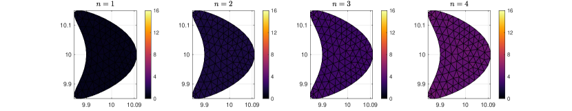
((b)) $\log_{10}(\kappa(\widetilde{\bf V}))$

Figure 2: Visualization of the condition numbers of the Vandermonde matrices $\bf V$ and $\widetilde{\bf V}$, associated with the quadrature nodes in the physical triangle $K$ and in the corresponding translated and scaled triangle $\widetilde{K}$, respectively, for all the elements $K$ making up an elongated domain. The color axis represents the decimal logarithm of the condition numbers. The translation/scaling procedure’s remarkable effectiveness is clearly evident in these results; for example, for $n=2$ we observe a $10^{7}$-fold reduction in the condition number and a $10^{12}$-fold reduction for $n=4$

.

We repeatedly use the following lemma, which is a direct adaptation of [16, Thm. 1] to our notation.

Lemma 3.3.

If ${\bf V}$ is nonsingular and $\left\|{\bf{V}}^{-1}\right\|\leq M$, then the set $\mathcal{Y}$ is $\Lambda$-poised with $\Lambda=\sqrt{q_{n}}M$ in the unit disk $B_{1}(\boldsymbol{0})$. Conversely, if the set ${\mathcal{Y}}$ is $\Lambda$-poised in the unit disk $B_{1}(\boldsymbol{0})$, then ${\bf{V}}$ is nonsingular and

$$\left\|{\bf{V}}^{-1}\right\|\leq\theta_{n}\Lambda$$

where $\theta_{n}>0$ is dependent on $n$ but independent of ${\mathcal{Y}}$ and $\Lambda$.

Theorem 3.4.

For a given $n\in\mathbb{N}$, let the nodes $\mathcal{I}_{n}$ be mapped from the Vioreanu-Rokhlin nodes $\widehat{\mathcal{I}}_{n}$ of order $n$ via a non-degenerate affine transformation $\boldsymbol{T}$. We have that the interpolation sets $\mathcal{I}_{n}$ and $\widetilde{\mathcal{I}}_{n}$ are poised in the normalized monomial basis $\{p_{\alpha}\}_{|\alpha|\leq n}$. Further, the associated multivariate Vandermonde matrix $\widetilde{\bf{V}}$ in Eq. 36 is invertible and its condition number satisfies the bound

(42) $$\kappa(\widetilde{\bf{V}})\leq\chi_{n}\left(1+\frac{h_{K}}{\rho_{K}}\right)^{n}\kappa(\widehat{\bf{V}}),$$

where $\chi_{n}$ is computable and depends only on $n$, and where $\widehat{\bf{V}}$ is the multivariate Vandermonde matrix in the normalized basis on $\widehat{\mathcal{I}}_{n}$.

Remark 3.5.

Explicit bounds on the “constant” $\theta_{n}$ in Lemma 3.3 can be computed; reference [16, Eq. (13)] provides the necessary ingredient for $n=2$, showing a path for bounding $\theta_{n}$ for larger $n$ as well. Concretely, while the quantity $\kappa(\widehat{\bf{V}})$ can be computed once and for all in the basis $\{p_{\alpha}\}_{|\alpha|\leq n}$ and is of very small size, the theorem represents a somewhat modest result because $\chi_{n}$ in Theorem 3.4 depends linearly on $\theta_{n}$ in Lemma 3.3, and the latter quantity admittedly, as reference [16] notes, likely grows as much as exponentially with $n$.

Proof 3.6.

As a first step, we estimate the ${\Lambda}$-poisedness of $\widehat{\mathcal{I}}_{n}$. It follows from Lemma 3.3, the identity $\|\widehat{\bf{V}}^{-1}\|=\kappa(\widehat{\bf{V}})\|\widehat{\bf{V}}\|^{-1}$, and the fact that $\|\widehat{\bf{V}}\|\geq 1$, that $\widehat{\mathcal{I}}_{n}$ is $\widehat{\Lambda}$-poised with

(43) $$\widehat{\Lambda}\coloneqq\sqrt{q_{n}}\kappa(\widehat{\bf{V}}),$$

where $\kappa(\widehat{\bf{V}})$ denotes the condition number of the multivariate Vandermonde matrix for the Vioreanu-Rokhlin nodes in the monomial basis.

We next study the effect of the mapping $\widetilde{\boldsymbol{T}}:\widehat{K}\to\widetilde{K}$ on the reference Lagrange-polynomial vector function, denoted $\widehat{\boldsymbol{\lambda}}=[\widehat{\lambda}_{1},\ldots,\widehat{\lambda}_{q_{n}}]^{\top}:\mathbb{R}^{2}\to\mathbb{R}^{q_{n}}$, which via the concept of $\Lambda$-poisedness introduced above, ultimately provides control on the condition number of the multivariate Vandermonde system. We first note that the polynomials

(44) $$\widetilde{\lambda}_{j}(\widetilde{\boldsymbol{x}})\coloneqq\widehat{\lambda}_{j}(\widetilde{\boldsymbol{T}}^{-1}(\widetilde{\boldsymbol{x}})),$$

in fact satisfy the Lagrange interpolation property $\widetilde{\lambda}_{j}(\widetilde{\boldsymbol{x}}_{i})=\delta_{ij}$, $i,j=1,\ldots,q_{n}$. An analogous statement holds for $\lambda_{j}(\boldsymbol{x})\coloneqq\widehat{\lambda}_{j}(\boldsymbol{T}^{-1}(\boldsymbol{x}))$. It follows that both $\widetilde{\mathcal{I}}_{n}$ and $\mathcal{I}_{n}$ are poised.

From Eq. 44 it follows that

$$\sup_{\widetilde{\boldsymbol{x}}\in B_{1}(\boldsymbol{0})}\left|\widetilde{\lambda}_{j}(\widetilde{\boldsymbol{x}})\right|=\sup_{\widetilde{\boldsymbol{x}}\in B_{1}(\boldsymbol{0})}\left|\widehat{\lambda}_{j}(\widetilde{\boldsymbol{T}}^{-1}(\widetilde{\boldsymbol{x}}))\right|\leq\sup_{\widehat{\boldsymbol{x}}\in B_{1+R}(\boldsymbol{0})}\left|\widehat{\lambda}_{j}(\widehat{\boldsymbol{x}})\right|,\quad j=1,\ldots,q_{n},$$

where we used the fact that $\widetilde{\boldsymbol{T}}^{-1}(B_{1}(\boldsymbol{0}))\subset B_{1+R}(\boldsymbol{0})$ where $R\coloneqq\widetilde{h}_{K}/\widetilde{\rho}_{K}=h_{K}/\rho_{K}$. This inclusion follows from the fact that $|\widehat{\boldsymbol{x}}|=|\widetilde{\boldsymbol{T}}^{-1}(\widetilde{\boldsymbol{x}})|=|{\bf A}\widetilde{\boldsymbol{x}}+\boldsymbol{b}|\leq\|{\bf A}\||\widetilde{\boldsymbol{x}}|+|\boldsymbol{b}|\leq R+1$ which we establish next in two parts. Indeed, $\left\|\bf A\right\|\leq\widehat{h}_{K}/\widetilde{\rho}_{K}\leq R$, a fact that itself results from [14, Lemma 2] that establishes the first inequality followed by use of the second inequality $\widehat{h}_{K}\leq\widetilde{h}_{K}$ which in turn follows from the fact that an equilateral triangle $\widehat{K}$ is the triangle having a minimum diameter among all triangles with a minimum bounding circle of unit radius. The bound $|\boldsymbol{b}|\leq 1$ used above, on the other hand, follows directly from the bijectivity of $\widetilde{\boldsymbol{T}}^{-1}:\widetilde{K}\to\widehat{K}$ together with the fact that, by construction, $\boldsymbol{0}\in\widetilde{K}$, which imply $\boldsymbol{b}=\widetilde{\boldsymbol{T}}^{-1}(\boldsymbol{0})\in\widehat{K}\subset\overline{B_{1}(\boldsymbol{0})}$.

It remains to estimate the supremum of $|\widehat{\lambda}_{j}|$ over $B_{1+R}(\boldsymbol{0})$, for which purpose we build upon the bound, that follows from the definition of $\Lambda$-poisedness Eq. 43, $|\widehat{\lambda}_{j}(\widehat{\boldsymbol{x}})|\leq\sqrt{q_{n}}\kappa(\widehat{\bf{V}})$ for $\widehat{\boldsymbol{x}}$ in the more limited region $B_{1}(\boldsymbol{0})$. To extend the estimate to $B_{1+R}(\boldsymbol{0})$ we use a Markov-type inequality that provides bounds on homogeneous sub-components of a polynomial relative to the norm of the polynomial on a more limited convex region such as a disk. Specifically, reference [23, Thm. 1] provides for a polynomial $Q(\boldsymbol{x})=\sum_{|\alpha|\leq n}d_{\alpha}\boldsymbol{x}^{\alpha}$, the bound

(45) $$\left|\sum_{|\alpha|=\ell}d_{\alpha}\boldsymbol{x}^{\alpha}\right|\leq B_{\ell}^{(n)}\left|\boldsymbol{x}\right|^{\ell}\sup_{\boldsymbol{y}\in B_{1}(\boldsymbol{0})}\left|Q(\boldsymbol{y})\right|,\quad\ell=0,\ldots,n,$$

where for a given $n$ the $(n+1)$-numbered constants $B_{\ell}^{(n)}$ are known explicitly (see [23]) and are related to the coefficients of Chebyshev polynomials of degree $n$. In our context, for a given $j\in\{1,\ldots,q_{n}\}$, choosing $Q(\widehat{\boldsymbol{x}})=\widehat{\lambda}_{j}(\widehat{\boldsymbol{x}})$ and summing over each of the homogeneous polynomials of degree $\ell=0,\ldots,n$ making up $\widehat{\lambda}_{j}$, we obtain $\widehat{\lambda}_{j}(\widehat{\boldsymbol{x}})=\sum_{\ell=0}^{n}\sum_{|\alpha|=\ell}d_{\alpha}\widehat{\boldsymbol{x}}^{\alpha}$. Then, employing the triangle inequality, and using Eq. 45, we readily find

$$\left|\widehat{\lambda}_{j}(\widehat{\boldsymbol{x}})\right|\leq\sum_{\ell=0}^{n}\left|\sum_{|\alpha|=\ell}d_{\alpha}\widehat{\boldsymbol{x}}^{\alpha}\right|\leq\left(\sup_{\boldsymbol{y}\in B_{1}(\boldsymbol{0})}\left|\widehat{\lambda}_{j}(\boldsymbol{y})\right|\right)\sum_{\ell=0}^{n}B_{\ell}^{(n)}|\widehat{\boldsymbol{x}}|^{\ell}\leq\left(\sup_{\boldsymbol{y}\in B_{1}(\boldsymbol{0})}\left|\widehat{\lambda}_{j}(\boldsymbol{y})\right|\right)\left(\max_{\ell=0,\ldots,n}B^{(n)}_{\ell}\right)\sum_{\ell=0}^{n}|\widehat{\boldsymbol{x}}|^{\ell}.$$

Letting $B^{(n)}=\max_{\ell=0,\ldots,n}B_{\ell}^{(n)}$ and taking supremum of the expressions above over $\widehat{\boldsymbol{x}}\in B_{1+R}(\boldsymbol{0})$ it hence follows that

$$\begin{split}\sup_{\widetilde{\boldsymbol{x}}\in B_{1}(\boldsymbol{0})}\left|\widetilde{\lambda}_{j}(\widetilde{\boldsymbol{x}})\right|&\leq\sup_{\widehat{\boldsymbol{x}}\in B_{1+R}(\boldsymbol{0})}\left|\widehat{\lambda}_{j}(\widehat{\boldsymbol{x}})\right|\leq 2B^{(n)}(1+R)^{n}\sup_{\boldsymbol{y}\in B_{1}(\boldsymbol{0})}\left|\widehat{\lambda}_{j}(\boldsymbol{y})\right|,\quad j=1,\ldots,q_{n},\end{split}$$

where we have used the fact that $\sum_{\ell=0}^{n}|\widehat{\boldsymbol{x}}|^{\ell}\leq\sum_{\ell=0}^{n}(1+R)^{\ell}=[(1+R)^{n+1}-1]/R\leq 2(1+R)^{n}$ which is in turn obtained from $R=h_{K}/\rho_{K}>1$ and $\widehat{\boldsymbol{x}}\in B_{1+R}(\boldsymbol{0})$. It follows immediately that the set $\widetilde{\mathcal{I}}_{n}$ is $\widetilde{\Lambda}$-poised with

(46) $$\widetilde{\Lambda}\coloneqq 2B^{(n)}(1+R)^{n}\sqrt{q_{n}}\kappa(\widehat{\bf{V}})\geq 2B^{(n)}(1+R)^{n}\sup_{\boldsymbol{y}\in B_{1}(\boldsymbol{0})}\|\widehat{\boldsymbol{\lambda}}(\boldsymbol{y})\|_{2}\geq\sup_{\widetilde{\boldsymbol{x}}\in B_{1}(\boldsymbol{0})}\|\widetilde{\boldsymbol{\lambda}}(\widetilde{\boldsymbol{x}})\|_{2}.$$

We have, further, from using Lemma 3.3 together with Eq. 46, the bound

(47) $$\left\|\widetilde{\bf V}^{-1}\right\|\leq\theta_{n}\widetilde{\Lambda}=2\theta_{n}B^{(n)}(1+R)^{n}\sqrt{q_{n}}\kappa(\widehat{\bf{V}}).$$

Here $\theta_{n}$ denotes the quantity in Lemma 3.3 (see also Remark 3.5). The result follows from this inequality in conjunction with the inequality, see [16, Eq. (9)], $\left\|\widetilde{\bf{V}}\right\|\leq q_{n}^{3/2}$, which eventually yields $\chi_{n}=2\theta_{n}q_{n}^{2}B^{(n)}$.

To showcase the remarkable effectiveness of the translation-and-scaling methodology in practical applications, we present Figure 2(b). This figure illustrates the ($\log_{10}$ of the) condition numbers of the direct and modified Vandermonde matrices, $\mathbf{V}$ and $\widetilde{\mathbf{V}}$, respectively, over a fixed triangulation of a kite-shaped domain $\Omega$ for various interpolation orders. Notably, these examples demonstrate a significant reduction in the condition number by several orders of magnitude, demonstrating the capabilities of the proposed methodology; smaller domains centered further away from the origin would make the contrast progressively starker. Finally, to assess the sharpness of the estimate (42), we present Figure 3 which displays the quotient $\kappa(\widetilde{\bf V})/\kappa(\widehat{\bf V})$ plotted against $1+h_{K}/\rho_{K}$ for matrices $\widetilde{\bf V}$ corresponding to 1000 triangles $K$ with random vertices uniformly distributed within $[-10,10]^{2}$ and for various interpolation orders. These results suggest that our bound (42) effectively captures the dependence of the condition number $\kappa(\widetilde{\bf V})$ on the triangle’s shape characterized here by the “aspect ratio” $h_{K}/\rho_{K}$.

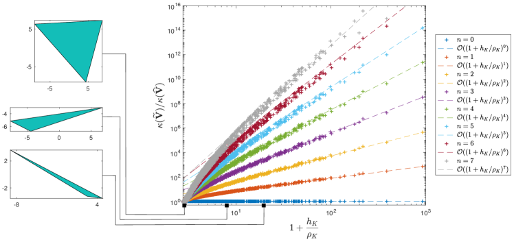
Figure 3: Dependence of the condition number $\kappa(\widetilde{\bf V})$ on the interpolation order $n$ and the triangle’s shape characterized by the “aspect ratio” $h_{K}/\rho_{K}$. Each of the data points marked by a colored plus sign (+) corresponds to a triangle $K$ with randomly generated vertices contained in $[-10,10]^{2}$. A total of 1000 triangles were used in this example, each tested for every $n$ in the study. The dashed lines mark the asymptotic behavior of the bound for $\kappa(\widetilde{\bf V})/\kappa(\widehat{\bf V})$ established in Theorem 3.4. A remarkable agreement between the empirical data and theoretical bound is observed.

3.2.4 Numerical quadrature accuracy for regularized volume integrals

This section examines the regularizing effect of the density interpolant on the volume potential evaluated at some point $\boldsymbol{x}\in K$, $K$ a (curvilinear) triangular element. Its relevance is that part of the method’s efficiency owes to the avoidance of the use of (near-)singular volumetric quadrature in the entirety of the domain, as explained in the preamble to Section 3.2. Indeed, we develop the arguments that allow us to restrict the use of nearly-singular quadrature (for layer potentials) to a bounded region close to the boundary and still control the error introduced by using generic quadratures meant for smooth functions on regularized volume integrals. In fact, the error estimates are optimal in the sense that they establish the same order of convergence as that would be achieved with the use of exact evaluation of the nearly-singular volume integrals—we stress that the required number of such evaluations would scale as $\mathcal{O}(1/h^{2})$. Moreover, the results in the numerical experiments closely match the theoretical rate of convergence.

We must account for contributions from both singular and near-singular integration and for these purposes it is helpful to handle integration regions separately, so we denote by $\Omega_{h}=\Omega_{h}(\boldsymbol{x})$ an $\mathcal{O}(h)$-sized neighborhood of $K\ni\boldsymbol{x}$, obtained, say, by querying all triangles that share (at least) a vertex with $K$. Writing the volume potential as

(48) $$\mathcal{V}_{k}\left[f\right](\boldsymbol{x})=\left(\int_{\Omega\setminus\Omega_{h}}+\int_{\Omega_{h}\setminus K}+\int_{K}\right)G_{k}(\boldsymbol{x},\boldsymbol{y})f(\boldsymbol{y})\,\mathrm{d}\boldsymbol{y},$$

the analysis that follows estimates the contribution of the latter two integrals for the potential $\mathcal{V}_{k}[f-f_{n}(\cdot;K)](\boldsymbol{x})$, where $f_{n}(\cdot;K)$ is the Lagrange interpolant of $f$ over $K\ni\boldsymbol{x}$. On the basis of the estimates that follow we could, for evaluation at a given $\boldsymbol{x}$, neglect all elements in the region $\Omega_{h}$ and retain an optimal order of convergence; in practice, for both simplicity and accuracy, only the contribution from $K$ will be discarded; cf. the punctured Green’s function definition in the second relation of Eq. 14. We recall the definitions Eq. 32 of the punctured volume potentials and for convenience write them in the form

$$\mathchoice{\mathop{\vbox{\halign{#\cr\kern 0.80002pt$\hss\leavevmode\resizebox{6.00003pt}{3.8889pt}{\rotatebox[origin={c}]{90.0}{(}}\hss$\crcr\nointerlineskip\cr$\hss\displaystyle\mathcal{V}\hss$\crcr}}}\limits}{\mathop{\vbox{\halign{#\cr\kern 0.80002pt$\hss\leavevmode\resizebox{6.00003pt}{3.8889pt}{\rotatebox[origin={c}]{90.0}{(}}\hss$\crcr\nointerlineskip\cr$\hss\textstyle\mathcal{V}\hss$\crcr}}}\limits}{\mathop{\vbox{\halign{#\cr\kern 0.80002pt$\hss\leavevmode\resizebox{4.20001pt}{2.72223pt}{\rotatebox[origin={c}]{90.0}{(}}\hss$\crcr\nointerlineskip\cr$\hss\scriptstyle\mathcal{V}\hss$\crcr}}}\limits}{\mathop{\vbox{\halign{#\cr\kern 0.80002pt$\hss\leavevmode\resizebox{3.0pt}{1.94444pt}{\rotatebox[origin={c}]{90.0}{(}}\hss$\crcr\nointerlineskip\cr$\hss\scriptscriptstyle\mathcal{V}\hss$\crcr}}}\limits}_{k}[f](\boldsymbol{x})=\left(\int_{\Omega\setminus\Omega_{h}}+\int_{\Omega_{h}\setminus K}\right)G_{k}(\boldsymbol{y},\boldsymbol{x})f(\boldsymbol{y})\,\mathrm{d}\boldsymbol{y}\,\,\mbox{and}\,\,\mathchoice{\mathop{\vbox{\halign{#\cr\kern 0.80002pt$\hss\leavevmode\resizebox{8.22226pt}{3.8889pt}{\rotatebox[origin={c}]{90.0}{(}}\hss$\crcr\nointerlineskip\cr$\hss\displaystyle\mathcal{W}\hss$\crcr}}}\limits}{\mathop{\vbox{\halign{#\cr\kern 0.80002pt$\hss\leavevmode\resizebox{8.22226pt}{3.8889pt}{\rotatebox[origin={c}]{90.0}{(}}\hss$\crcr\nointerlineskip\cr$\hss\textstyle\mathcal{W}\hss$\crcr}}}\limits}{\mathop{\vbox{\halign{#\cr\kern 0.80002pt$\hss\leavevmode\resizebox{5.75558pt}{2.72223pt}{\rotatebox[origin={c}]{90.0}{(}}\hss$\crcr\nointerlineskip\cr$\hss\scriptstyle\mathcal{W}\hss$\crcr}}}\limits}{\mathop{\vbox{\halign{#\cr\kern 0.80002pt$\hss\leavevmode\resizebox{4.11113pt}{1.94444pt}{\rotatebox[origin={c}]{90.0}{(}}\hss$\crcr\nointerlineskip\cr$\hss\scriptscriptstyle\mathcal{W}\hss$\crcr}}}\limits}_{k}[f](\boldsymbol{x})=\left(\int_{\Omega\setminus\Omega_{h}}+\int_{\Omega_{h}\setminus K}\right)\nabla_{\boldsymbol{y}}G_{k}(\boldsymbol{x},\boldsymbol{y})\cdot\mathbf{f}(\boldsymbol{y})\,\mathrm{d}\boldsymbol{y}.$$

(Recall from Section 3.2 that $\mathchoice{\mathop{\vbox{\halign{#\cr\kern 0.80002pt$\hss\leavevmode\resizebox{6.00003pt}{3.8889pt}{\rotatebox[origin={c}]{90.0}{(}}\hss$\crcr\nointerlineskip\cr$\hss\displaystyle\mathcal{V}\hss$\crcr}}}\limits}{\mathop{\vbox{\halign{#\cr\kern 0.80002pt$\hss\leavevmode\resizebox{6.00003pt}{3.8889pt}{\rotatebox[origin={c}]{90.0}{(}}\hss$\crcr\nointerlineskip\cr$\hss\textstyle\mathcal{V}\hss$\crcr}}}\limits}{\mathop{\vbox{\halign{#\cr\kern 0.80002pt$\hss\leavevmode\resizebox{4.20001pt}{2.72223pt}{\rotatebox[origin={c}]{90.0}{(}}\hss$\crcr\nointerlineskip\cr$\hss\scriptstyle\mathcal{V}\hss$\crcr}}}\limits}{\mathop{\vbox{\halign{#\cr\kern 0.80002pt$\hss\leavevmode\resizebox{3.0pt}{1.94444pt}{\rotatebox[origin={c}]{90.0}{(}}\hss$\crcr\nointerlineskip\cr$\hss\scriptscriptstyle\mathcal{V}\hss$\crcr}}}\limits}_{k}^{h,m}$ and $\mathchoice{\mathop{\vbox{\halign{#\cr\kern 0.80002pt$\hss\leavevmode\resizebox{8.22226pt}{3.8889pt}{\rotatebox[origin={c}]{90.0}{(}}\hss$\crcr\nointerlineskip\cr$\hss\displaystyle\mathcal{W}\hss$\crcr}}}\limits}{\mathop{\vbox{\halign{#\cr\kern 0.80002pt$\hss\leavevmode\resizebox{8.22226pt}{3.8889pt}{\rotatebox[origin={c}]{90.0}{(}}\hss$\crcr\nointerlineskip\cr$\hss\textstyle\mathcal{W}\hss$\crcr}}}\limits}{\mathop{\vbox{\halign{#\cr\kern 0.80002pt$\hss\leavevmode\resizebox{5.75558pt}{2.72223pt}{\rotatebox[origin={c}]{90.0}{(}}\hss$\crcr\nointerlineskip\cr$\hss\scriptstyle\mathcal{W}\hss$\crcr}}}\limits}{\mathop{\vbox{\halign{#\cr\kern 0.80002pt$\hss\leavevmode\resizebox{4.11113pt}{1.94444pt}{\rotatebox[origin={c}]{90.0}{(}}\hss$\crcr\nointerlineskip\cr$\hss\scriptscriptstyle\mathcal{W}\hss$\crcr}}}\limits}_{k}^{h,m}$ denote numerical quadrature approximations to these operators over $\mathcal{T}_{h}$ with a quadrature rule capable of integrating polynomials of total degree at most $m$.)

The theorem applies for evaluation on subsets of the plane that are interior to an element with respect to other elements of the mesh, an idea made precise in the next definition.

Definition 3.7.

Consider a family of triangulations of $\Omega$ denoted by $\mathcal{T}=\{\mathcal{T}_{h}\}_{h>0}$ with $h$ denoting the maximum element size in $\mathcal{T}_{h}$, and let $\mathcal{S}_{h}=\bigcup_{K\in\mathcal{T}_{h}}\partial K$. A family of evaluation point sets $\mathcal{E}=\{\mathcal{E}_{h}\}_{h>0}$, $\mathcal{E}_{h}\subset\overline{\Omega}$ for all $h>0$, possibly intersecting the boundary $\Gamma=\partial\Omega$, is called well-separated with respect to $\mathcal{T}$ if

(49) $$d_{\mathcal{T},\mathcal{E}}\coloneqq\inf_{h>0}\,\,\inf_{\begin{subarray}{c}\boldsymbol{y}\in\mathcal{S}_{h}\setminus\Gamma\\ \boldsymbol{x}\in\mathcal{E}_{h}\end{subarray}}\frac{|\boldsymbol{x}-\boldsymbol{y}|}{h}>0.$$

A typical example is evaluation at the point set consisting of (interior) Vioreanu-Rokhlin interpolation/quadrature nodes: the theorem thus estimates the error in the volume potential evaluated at all the interpolation/quadrature points $\left\{{\boldsymbol{\xi}_{j}}\right\}_{j=1}^{N}$, $N=Lq_{n}$. (Indeed, any set of interior points on $\widehat{K}$ leads to a well-separated family of evaluation points over the triangulation, as the proof of the following proposition shows.) Another use-case of the definition would be the evaluation at point-sets laying on the boundary $\Gamma=\partial\Omega$, e.g. for the solution of boundary value problems.

Proposition 3.8.

Let $\mathcal{T}=\{\mathcal{T}_{h}\}_{h>0}$ be a quasi-uniform and shape-regular family of triangulations (in the sense of [50]) of $\Omega$. The family $\mathcal{E}=\{\mathcal{E}_{h}\}_{h>0}$ with $\mathcal{E}_{h}$ being a set of interior quadrature nodes over a triangulation $\mathcal{T}_{h}\subset\mathcal{T}$ of $\Omega$, is a well-separated family of evaluation point sets with respect to $\mathcal{T}$.

Proof 3.9.

Let $\widehat{\mathcal{Q}}$ denote the quadrature nodes on $\widehat{K}$ and set $\widehat{\delta}=\inf_{\widehat{\boldsymbol{y}}\in\partial\widehat{K},\widehat{\boldsymbol{x}}\in\widehat{\mathcal{Q}}}|\widehat{\boldsymbol{x}}-\widehat{\boldsymbol{y}}|>0$, which is clearly independent of the families $\mathcal{T}$ and $\mathcal{E}$. Consider a triangle $K\in\mathcal{T}_{h}$ and let $\boldsymbol{T}:\widehat{K}\to K$ be the affine transformation $\boldsymbol{T}(\widehat{\boldsymbol{x}})=\boldsymbol{A}\widehat{\boldsymbol{x}}+\boldsymbol{b}$. Then $\mathcal{Q}=\boldsymbol{T}(\widehat{\mathcal{Q}})$ equals the set of quadrature nodes contained in $K$. From the bijectivity of $\boldsymbol{T}$ and [14, Lem. 2] we have

$$\widehat{\delta}\leq|\boldsymbol{T}^{-1}(\boldsymbol{x})-\boldsymbol{T}^{-1}(\boldsymbol{y})|\leq\|\boldsymbol{A}^{-1}\||\boldsymbol{x}-\boldsymbol{y}|\leq\frac{\widehat{h}}{\rho_{K}}|\boldsymbol{x}-\boldsymbol{y}|\quad\text{for all}\quad\boldsymbol{x}\in\mathcal{Q}\subset K,\,\boldsymbol{y}\in\partial K.$$

Now, using the fact that $\rho_{K}^{-1}\leq\kappa_{\mathcal{T}}/h_{K}$ and that $h_{K}^{-1}\leq q_{\mathcal{T}}/h$, we obtain $\rho_{K}^{-1}\leq\kappa_{\mathcal{T}}q_{\mathcal{T}}/h$. Here

$$\kappa_{\mathcal{T}}=\sup_{h>0}\max_{K\in\mathcal{T}_{h}}\frac{h_{K}}{\rho_{K}}\quad\text{and}\quad q_{\mathcal{T}}=\sup_{h>0}\frac{h}{\min_{K\in\mathcal{T}_{h}}h_{K}},$$

which by the shape-regularity and quasi-uniform assumptions on $\mathcal{T}$, are finite constants. It hence follows from the inequalities above that

$$\widehat{\delta}\leq\widehat{h}k_{\mathcal{T}}q_{\mathcal{T}}\frac{|\boldsymbol{x}-\boldsymbol{y}|}{h}\quad\text{for all}\quad\boldsymbol{x}\in\mathcal{Q}\subset K,\,\boldsymbol{y}\in\partial K.$$

Therefore, taking infimum over all the points $\boldsymbol{x}\in\mathcal{E}_{h}$ and $\boldsymbol{y}\in S_{h}$, and then infimum over all the triangulations $\mathcal{T}_{h}$, we arrive at

$$d_{\mathcal{T},\mathcal{E}}\geq\frac{\widehat{\delta}}{\widehat{h}}\frac{1}{k_{\mathcal{T}}q_{\mathcal{T}}}>0.$$

The proof is now complete.

Remark 3.10.

Similar statements can be easily made for triangulations including curved triangles as well as for families of evaluation point sets $\mathcal{E}$ that lay on $\Gamma$ (and yet separated from $\mathcal{S}_{h}$).

Theorem 3.11.

Let the respective (positive weight) quadrature and interpolation orders $m,n\in\mathbb{N}_{0}$ and the wavenumber $k\in\mathbb{C}$ be given and let $\mathcal{T}=\left\{\mathcal{T}_{h}\right\}_{h>0}$ denote a family of triangulations of $\Omega$. Let $\mathcal{E}=\{\mathcal{E}_{h}\}_{h>0}$ be a family of well-separated evaluation point sets for $\mathcal{T}$, and denote by $f_{n}(\cdot;K)$ (resp. $\mathbf{f}_{n}(\cdot;K)$) the Lagrange polynomial interpolant of $f\in C^{m+1}(\overline{\Omega})$ (resp. $\mathbf{f}\in[C^{m+1}(\overline{\Omega})]^{2}$) with interpolation in some $K\in\mathcal{T}_{h}$ enforced on the associated interpolation node-set $\mathcal{I}_{n}\subset K$. It holds that

(50) $$\left|\mathcal{V}_{k}\left[f-f_{n}(\cdot;K)\right](\boldsymbol{x})-\mathchoice{\mathop{\vbox{\halign{#\cr\kern 0.80002pt$\hss\leavevmode\resizebox{6.00003pt}{3.8889pt}{\rotatebox[origin={c}]{90.0}{(}}\hss$\crcr\nointerlineskip\cr$\hss\displaystyle\mathcal{V}\hss$\crcr}}}\limits}{\mathop{\vbox{\halign{#\cr\kern 0.80002pt$\hss\leavevmode\resizebox{6.00003pt}{3.8889pt}{\rotatebox[origin={c}]{90.0}{(}}\hss$\crcr\nointerlineskip\cr$\hss\textstyle\mathcal{V}\hss$\crcr}}}\limits}{\mathop{\vbox{\halign{#\cr\kern 0.80002pt$\hss\leavevmode\resizebox{4.20001pt}{2.72223pt}{\rotatebox[origin={c}]{90.0}{(}}\hss$\crcr\nointerlineskip\cr$\hss\scriptstyle\mathcal{V}\hss$\crcr}}}\limits}{\mathop{\vbox{\halign{#\cr\kern 0.80002pt$\hss\leavevmode\resizebox{3.0pt}{1.94444pt}{\rotatebox[origin={c}]{90.0}{(}}\hss$\crcr\nointerlineskip\cr$\hss\scriptscriptstyle\mathcal{V}\hss$\crcr}}}\limits}_{k}^{h,m}\left[f-f_{n}(\cdot;K)\right](\boldsymbol{x})\right|\leq C^{(1)}_{\mathcal{V}}h^{n+3}|\log{h}|+C^{(2)}_{\mathcal{V}}h^{m+1},\quad\boldsymbol{x}\in K\cap\mathcal{E}_{h},$$

where $C^{(1)}_{\mathcal{V}}$ and $C^{(2)}_{\mathcal{V}}$ are positive constants independent of $h$ but dependent on $f$, $k$ and $d_{\mathcal{T},\mathcal{E}}$, and it holds that

(51) $$\left|\mathcal{W}_{k}\left[\mathbf{f}-\mathbf{f}_{n}(\cdot;K)\right](\boldsymbol{x})-\mathchoice{\mathop{\vbox{\halign{#\cr\kern 0.80002pt$\hss\leavevmode\resizebox{8.22226pt}{3.8889pt}{\rotatebox[origin={c}]{90.0}{(}}\hss$\crcr\nointerlineskip\cr$\hss\displaystyle\mathcal{W}\hss$\crcr}}}\limits}{\mathop{\vbox{\halign{#\cr\kern 0.80002pt$\hss\leavevmode\resizebox{8.22226pt}{3.8889pt}{\rotatebox[origin={c}]{90.0}{(}}\hss$\crcr\nointerlineskip\cr$\hss\textstyle\mathcal{W}\hss$\crcr}}}\limits}{\mathop{\vbox{\halign{#\cr\kern 0.80002pt$\hss\leavevmode\resizebox{5.75558pt}{2.72223pt}{\rotatebox[origin={c}]{90.0}{(}}\hss$\crcr\nointerlineskip\cr$\hss\scriptstyle\mathcal{W}\hss$\crcr}}}\limits}{\mathop{\vbox{\halign{#\cr\kern 0.80002pt$\hss\leavevmode\resizebox{4.11113pt}{1.94444pt}{\rotatebox[origin={c}]{90.0}{(}}\hss$\crcr\nointerlineskip\cr$\hss\scriptscriptstyle\mathcal{W}\hss$\crcr}}}\limits}_{k}^{h,m}\left[\mathbf{f}-\mathbf{f}_{n}(\cdot;K)\right](\boldsymbol{x})\right|\leq C^{(1)}_{\mathcal{W}}h^{n+2}+C^{(2)}_{\mathcal{W}}h^{m+1},\quad\boldsymbol{x}\in K\cap\mathcal{E}_{h},$$

where $C^{(1)}_{\mathcal{W}}$ and $C^{(2)}_{\mathcal{W}}$ are positive constants independent of $h$ but dependent on $f$, $k$ and $d_{\mathcal{T},\mathcal{E}}$.

Remark 3.12.

For interpolation orders $n\geq 2$, the Vioreanu-Rokhlin rules satisfy $m\geq n+2$ [57, Tab. 5.1], so the error estimate Eq. 50 in such cases simplifies to

(52) $$\left|\mathcal{V}_{k}\left[f-f_{n}(\cdot;K)\right](\boldsymbol{x})-\mathchoice{\mathop{\vbox{\halign{#\cr\kern 0.80002pt$\hss\leavevmode\resizebox{6.00003pt}{3.8889pt}{\rotatebox[origin={c}]{90.0}{(}}\hss$\crcr\nointerlineskip\cr$\hss\displaystyle\mathcal{V}\hss$\crcr}}}\limits}{\mathop{\vbox{\halign{#\cr\kern 0.80002pt$\hss\leavevmode\resizebox{6.00003pt}{3.8889pt}{\rotatebox[origin={c}]{90.0}{(}}\hss$\crcr\nointerlineskip\cr$\hss\textstyle\mathcal{V}\hss$\crcr}}}\limits}{\mathop{\vbox{\halign{#\cr\kern 0.80002pt$\hss\leavevmode\resizebox{4.20001pt}{2.72223pt}{\rotatebox[origin={c}]{90.0}{(}}\hss$\crcr\nointerlineskip\cr$\hss\scriptstyle\mathcal{V}\hss$\crcr}}}\limits}{\mathop{\vbox{\halign{#\cr\kern 0.80002pt$\hss\leavevmode\resizebox{3.0pt}{1.94444pt}{\rotatebox[origin={c}]{90.0}{(}}\hss$\crcr\nointerlineskip\cr$\hss\scriptscriptstyle\mathcal{V}\hss$\crcr}}}\limits}_{k}^{h,m}\left[f-f_{n}(\cdot,K)\right](\boldsymbol{x})\right|\leq C_{\mathcal{V}}h^{n+3}|\log h|,\quad\boldsymbol{x}\in K\cap\mathcal{E}_{h},$$

for some constant $C_{\mathcal{V}}>0$. Similarly, since for $n\geq 1$ it holds that $m\geq n+1$, so the the error estimate Eq. 51 simplifies to

(53) $$\left|\mathcal{W}_{k}\left[\mathbf{f}-\mathbf{f}_{n}(\cdot;K)\right](\boldsymbol{x})-\mathchoice{\mathop{\vbox{\halign{#\cr\kern 0.80002pt$\hss\leavevmode\resizebox{8.22226pt}{3.8889pt}{\rotatebox[origin={c}]{90.0}{(}}\hss$\crcr\nointerlineskip\cr$\hss\displaystyle\mathcal{W}\hss$\crcr}}}\limits}{\mathop{\vbox{\halign{#\cr\kern 0.80002pt$\hss\leavevmode\resizebox{8.22226pt}{3.8889pt}{\rotatebox[origin={c}]{90.0}{(}}\hss$\crcr\nointerlineskip\cr$\hss\textstyle\mathcal{W}\hss$\crcr}}}\limits}{\mathop{\vbox{\halign{#\cr\kern 0.80002pt$\hss\leavevmode\resizebox{5.75558pt}{2.72223pt}{\rotatebox[origin={c}]{90.0}{(}}\hss$\crcr\nointerlineskip\cr$\hss\scriptstyle\mathcal{W}\hss$\crcr}}}\limits}{\mathop{\vbox{\halign{#\cr\kern 0.80002pt$\hss\leavevmode\resizebox{4.11113pt}{1.94444pt}{\rotatebox[origin={c}]{90.0}{(}}\hss$\crcr\nointerlineskip\cr$\hss\scriptscriptstyle\mathcal{W}\hss$\crcr}}}\limits}_{k}^{h,m}\left[\mathbf{f}-\mathbf{f}_{n}(\cdot;K)\right](\boldsymbol{x})\right|\leq C_{\mathcal{W}}h^{n+2},\quad\boldsymbol{x}\in K\cap\mathcal{E}_{h},$$

for some constant $C_{\mathcal{W}}>0$. (Estimates Eq. 50 and Eq. 51 yield concrete error estimates when $n<2$ via the relations [57, Tab. 5.1] $m=1$ when $n=0$ and $m=2$ when $n=1$; note that the case $n=1$ happens to be, comparing to Figure 5, the case where super-convergence is observed in numerical experiments for the $\mathcal{V}_{k}$ operator.) As a consequence, the analysis that follows shows, for $\mathcal{V}_{k}$ and $n\geq 2$ or for $\mathcal{W}_{k}$ and $n\geq 1$, that these estimates for the numerical quadrature evaluation of the potential of the regularized volume integral yield precisely the order of accuracy in Eq. 57 and Eq. 58, respectively, of the regularization error alone—that is, the approximation error introduced by neglecting the regularized weakly-singular integral over $K$.

Proof 3.13.

The proof, with exposition primarily restricted to the operator $\mathcal{V}_{k}$ and relevant differences for the $\mathcal{W}_{k}$ case mentioned as needed, proceeds by first showing that the error incurred by neglecting the weakly-singular integral over $K$ in $\mathchoice{\mathop{\vbox{\halign{#\cr\kern 0.80002pt$\hss\leavevmode\resizebox{6.00003pt}{3.8889pt}{\rotatebox[origin={c}]{90.0}{(}}\hss$\crcr\nointerlineskip\cr$\hss\displaystyle\mathcal{V}\hss$\crcr}}}\limits}{\mathop{\vbox{\halign{#\cr\kern 0.80002pt$\hss\leavevmode\resizebox{6.00003pt}{3.8889pt}{\rotatebox[origin={c}]{90.0}{(}}\hss$\crcr\nointerlineskip\cr$\hss\textstyle\mathcal{V}\hss$\crcr}}}\limits}{\mathop{\vbox{\halign{#\cr\kern 0.80002pt$\hss\leavevmode\resizebox{4.20001pt}{2.72223pt}{\rotatebox[origin={c}]{90.0}{(}}\hss$\crcr\nointerlineskip\cr$\hss\scriptstyle\mathcal{V}\hss$\crcr}}}\limits}{\mathop{\vbox{\halign{#\cr\kern 0.80002pt$\hss\leavevmode\resizebox{3.0pt}{1.94444pt}{\rotatebox[origin={c}]{90.0}{(}}\hss$\crcr\nointerlineskip\cr$\hss\scriptscriptstyle\mathcal{V}\hss$\crcr}}}\limits}_{k}$ is an $\mathcal{O}(h^{n+3}\log h)$ quantity as $h\to 0$, and then next that the near-singular volume integrals over each of the elements within the neighborhood $\Omega_{h}$ of $\boldsymbol{x}$ are each $\mathcal{O}(h^{n+3}\log h)$ quantities so that the integral over $\Omega_{h}\setminus K$ approximates the integral over $\Omega_{h}$ with errors that behave as $\mathcal{O}(h^{n+3}\log h)$ as $h\to 0$. Then we finally consider the error from numerical quadrature that arises both from integration on the elements in the near-field $\Omega_{h}\setminus K$ and from the elements in the far-field $\Omega\setminus\Omega_{h}$. Throughout this proof, ${C}_{j}$, $j=0,\ldots,6$ will denote positive constants independent of $h$.

Let $\boldsymbol{x}\in K\cap\mathcal{E}_{h}$ denote a fixed evaluation point. In what follows the Lagrange interpolation error estimate [54, Thm. 1] (that holds since the interpolant here is polynomial and thus easily satisfies the required uniformity condition needed there) will prove useful; it provides (cf. also [14, Thm. 2])

(54) $$\left|f(\boldsymbol{y})-f_{n}(\boldsymbol{y};K)\right|\leq{C}_{0}h^{n+1}\quad\mbox{for all}\quad\boldsymbol{y}\in\Omega_{h}(\boldsymbol{x}),$$

and, for vector-valued functions the corresponding estimate

(55) $$|\mathbf{f}(\boldsymbol{y})-\mathbf{f}_{n}(\boldsymbol{y};K)|\leq{C}_{1}h^{n+1}\quad\mbox{for all}\quad\boldsymbol{y}\in\Omega_{h}(\boldsymbol{x}),$$

where ${C}_{0}$ and ${C}_{1}$ denote constants independent of $h$ but possibly dependent on the quotient of the diameter of $\Omega_{h}$ and $h$. Note that these estimates hold not merely on $K$ but as well over an $\mathcal{O}(h)$ neighborhood; indeed, the result of [14, Thm. 2] can be applied over the entirety of $\Omega_{h}$ with interpolation conditions enforced at $\mathcal{I}_{n}\subset K$.

The first step of the proof provides bounds on components of the regularized volume potential. Considering each of the integrals over the elements of $\Omega_{h}$, we have from a change to polar variables centered at $\boldsymbol{x}\in K\cap\mathcal{E}_{h}\subset\Omega_{h}$ and the bound Eq. 54, the estimate

(56) $$\bigg{|}\,\int_{\Omega_{h}}G_{k}(\boldsymbol{x},\boldsymbol{y})\left[f(\boldsymbol{y})-f_{n}(\boldsymbol{y};K)\right]\,\mathrm{d}\boldsymbol{y}\,\bigg{|}\leq\int_{\Omega_{h}}\left|G_{k}(\boldsymbol{x},\boldsymbol{y})\left[f(\boldsymbol{y})-f_{n}(\boldsymbol{y};K)\right]\right|\,\mathrm{d}\boldsymbol{y}\leq{C}_{2}h^{n+3}|\log{h}|,$$

which in view of the fact that $K\subset\Omega_{h}(\boldsymbol{x})$ implies that

(57) $$\left|\mathcal{V}_{k}\left[f-f_{n}(\cdot;K)\right](\boldsymbol{x})-\mathchoice{\mathop{\vbox{\halign{#\cr\kern 0.80002pt$\hss\leavevmode\resizebox{6.00003pt}{3.8889pt}{\rotatebox[origin={c}]{90.0}{(}}\hss$\crcr\nointerlineskip\cr$\hss\displaystyle\mathcal{V}\hss$\crcr}}}\limits}{\mathop{\vbox{\halign{#\cr\kern 0.80002pt$\hss\leavevmode\resizebox{6.00003pt}{3.8889pt}{\rotatebox[origin={c}]{90.0}{(}}\hss$\crcr\nointerlineskip\cr$\hss\textstyle\mathcal{V}\hss$\crcr}}}\limits}{\mathop{\vbox{\halign{#\cr\kern 0.80002pt$\hss\leavevmode\resizebox{4.20001pt}{2.72223pt}{\rotatebox[origin={c}]{90.0}{(}}\hss$\crcr\nointerlineskip\cr$\hss\scriptstyle\mathcal{V}\hss$\crcr}}}\limits}{\mathop{\vbox{\halign{#\cr\kern 0.80002pt$\hss\leavevmode\resizebox{3.0pt}{1.94444pt}{\rotatebox[origin={c}]{90.0}{(}}\hss$\crcr\nointerlineskip\cr$\hss\scriptscriptstyle\mathcal{V}\hss$\crcr}}}\limits}_{k}\left[f-f_{n}(\cdot;K)\right](\boldsymbol{x})\right|\leq{C}_{2}h^{n+3}|\log{h}|.$$

In a similar vein, it is easy to see that

(58) $$\left|\mathcal{W}_{k}\left[\mathbf{f}-\mathbf{f}_{n}(\cdot;K)\right](\boldsymbol{x})-\mathchoice{\mathop{\vbox{\halign{#\cr\kern 0.80002pt$\hss\leavevmode\resizebox{8.22226pt}{3.8889pt}{\rotatebox[origin={c}]{90.0}{(}}\hss$\crcr\nointerlineskip\cr$\hss\displaystyle\mathcal{W}\hss$\crcr}}}\limits}{\mathop{\vbox{\halign{#\cr\kern 0.80002pt$\hss\leavevmode\resizebox{8.22226pt}{3.8889pt}{\rotatebox[origin={c}]{90.0}{(}}\hss$\crcr\nointerlineskip\cr$\hss\textstyle\mathcal{W}\hss$\crcr}}}\limits}{\mathop{\vbox{\halign{#\cr\kern 0.80002pt$\hss\leavevmode\resizebox{5.75558pt}{2.72223pt}{\rotatebox[origin={c}]{90.0}{(}}\hss$\crcr\nointerlineskip\cr$\hss\scriptstyle\mathcal{W}\hss$\crcr}}}\limits}{\mathop{\vbox{\halign{#\cr\kern 0.80002pt$\hss\leavevmode\resizebox{4.11113pt}{1.94444pt}{\rotatebox[origin={c}]{90.0}{(}}\hss$\crcr\nointerlineskip\cr$\hss\scriptscriptstyle\mathcal{W}\hss$\crcr}}}\limits}_{k}\left[\mathbf{f}-\mathbf{f}_{n}(\cdot;K)\right](\boldsymbol{x})\right|\leq{C}_{3}h^{n+2},$$

where we used the fact $|\nabla_{\boldsymbol{y}}G_{k}(\boldsymbol{x},\boldsymbol{y})|=\mathcal{O}(h^{-1})$ as $h\to 0$ for $\boldsymbol{x},\boldsymbol{y}\in K$.

Similarly, since $\Omega_{h}\setminus K\subset\Omega_{h}$ we get from the latter inequality of Eq. 56 the bound

(59) $$\begin{split}\bigg{|}\,\int_{\Omega_{h}\setminus K}G_{k}(\boldsymbol{x},\boldsymbol{y})\left[f(\boldsymbol{y})-f_{n}(\boldsymbol{y};K)\right]\,\mathrm{d}\boldsymbol{y}\,\bigg{|}&\leq{C}_{2}h^{n+3}|\log{h}|\end{split}$$

and a similar argument for $\mathcal{W}_{k}$ yields

(60) $$\bigg{|}\,\int_{\Omega_{h}\setminus K}\nabla_{\boldsymbol{y}}G_{k}(\boldsymbol{x},\boldsymbol{y})\cdot\left[\mathbf{f}(\boldsymbol{y})-\mathbf{f}_{n}(\boldsymbol{y};K)\right]\,\mathrm{d}\boldsymbol{y}\,\bigg{|}\leq{C}_{3}h^{n+2}.$$

Turning to numerical quadratures, recall that the numerical quadrature rule exactly integrates polynomials up to total degree $m$ which implies that the integral of a function $\phi\in C^{m+1}(\Omega\setminus\Omega_{h})$ can be computed with an error that can be bounded [31] by

(61) $$\bigg{|}\,\int_{\Omega\setminus\Omega_{h}}\phi(\boldsymbol{y})\,\mathrm{d}\boldsymbol{y}-\sum_{\boldsymbol{\xi}_{j}\in\Omega\setminus\Omega_{h}}\omega_{j}\phi(\boldsymbol{\xi}_{j})\,\bigg{|}\leq{C}_{4}h^{m+1}.$$

For the elements comprising $\Omega_{h}\setminus K$, using Eq. 59 and Eq. 54 in conjunction with the triangle inequality, we find

(62) $$\begin{split}\bigg{|}\,\int_{\Omega_{h}\setminus K}G_{k}(\boldsymbol{x},\boldsymbol{y})\left[f(\boldsymbol{y})\;-\right.&\left.f_{n}(\boldsymbol{y};K)\right]\,\mathrm{d}\boldsymbol{y}-\sum_{\boldsymbol{\xi}_{j}\in\Omega_{h}\setminus K}\omega_{j}G_{k}(\boldsymbol{x},\boldsymbol{\xi}_{j})\left[f(\boldsymbol{\xi}_{j})-f_{n}(\boldsymbol{\xi}_{j};K)\right]\,\bigg{|}\leq\\ &\leq{C}_{2}h^{n+3}|\log{h}|+{C}_{0}h^{n+1}\max_{\begin{subarray}{c}\boldsymbol{\xi}_{j}\in\Omega_{h}\setminus K\end{subarray}}\left|G_{k}(\boldsymbol{x},\boldsymbol{\xi}_{j})\right|\sum_{\boldsymbol{\xi}_{j}\in\Omega_{h}\setminus K}\omega_{j}\\ &\leq C_{5}h^{n+3}|\log{h}|,\end{split}$$

where the inequalities above follow because, firstly, the quadrature rule has positive weights that satisfy $\sum_{\boldsymbol{\xi}_{j}\in\Omega_{h}\setminus K}\omega_{j}\lesssim h^{2}$ and secondly, since $\boldsymbol{x}\in\mathcal{E}_{h}$ lies at a distance from $\Omega_{h}\setminus K$ that scales linearly with $h$, $\max_{\boldsymbol{\xi}_{j}\in\Omega_{h}\setminus K}\left|G_{k}(\boldsymbol{x},\boldsymbol{\xi}_{j})\right|\lesssim|\log{h}|$, with an implied constant dependent on $d_{\mathcal{T},{\mathcal{E}}}$ (see Definition 3.7).

In a similar vein for the $\mathchoice{\mathop{\vbox{\halign{#\cr\kern 0.80002pt$\hss\leavevmode\resizebox{8.22226pt}{3.8889pt}{\rotatebox[origin={c}]{90.0}{(}}\hss$\crcr\nointerlineskip\cr$\hss\displaystyle\mathcal{W}\hss$\crcr}}}\limits}{\mathop{\vbox{\halign{#\cr\kern 0.80002pt$\hss\leavevmode\resizebox{8.22226pt}{3.8889pt}{\rotatebox[origin={c}]{90.0}{(}}\hss$\crcr\nointerlineskip\cr$\hss\textstyle\mathcal{W}\hss$\crcr}}}\limits}{\mathop{\vbox{\halign{#\cr\kern 0.80002pt$\hss\leavevmode\resizebox{5.75558pt}{2.72223pt}{\rotatebox[origin={c}]{90.0}{(}}\hss$\crcr\nointerlineskip\cr$\hss\scriptstyle\mathcal{W}\hss$\crcr}}}\limits}{\mathop{\vbox{\halign{#\cr\kern 0.80002pt$\hss\leavevmode\resizebox{4.11113pt}{1.94444pt}{\rotatebox[origin={c}]{90.0}{(}}\hss$\crcr\nointerlineskip\cr$\hss\scriptscriptstyle\mathcal{W}\hss$\crcr}}}\limits}_{k}$ kernel, using the triangle inequality and Eq. 60 together with the estimate Eq. 55 yields the bound

(63) $$\begin{split}\left|\int_{\Omega_{h}\setminus K}\nabla_{\boldsymbol{y}}G_{k}(\boldsymbol{x},\boldsymbol{y})\cdot\left[\mathbf{f}(\boldsymbol{y})\;-\right.\right.&\left.\left.\mathbf{f}_{n}(\boldsymbol{y};K)\right]\,\mathrm{d}\boldsymbol{y}-\sum_{\boldsymbol{\xi}_{j}\in\Omega_{h}\setminus K}\omega_{j}\nabla_{\boldsymbol{y}}G_{k}(\boldsymbol{x},\boldsymbol{\xi}_{j})\cdot\left[\mathbf{f}(\boldsymbol{\xi}_{j})-\mathbf{f}_{n}(\boldsymbol{\xi}_{j};K)\right]\right|\leq\\ &\leq C_{3}h^{n+2}+C_{1}h^{n+1}\max_{\begin{subarray}{c}\boldsymbol{\xi}_{j}\in\Omega_{h}\setminus K\end{subarray}}\left|\nabla_{\boldsymbol{y}}G_{k}(\boldsymbol{x},\boldsymbol{\xi}_{j})\right|\sum_{\boldsymbol{\xi}_{j}\in\Omega_{h}\setminus K}\omega_{j}\\ &\leq{C}_{6}h^{n+2},\end{split}$$

where the last inequality follows because, recalling $\boldsymbol{x}\in\mathcal{E}_{h}$, $\max_{\boldsymbol{\xi}_{j}\in\Omega_{h}\setminus K}\left|\nabla_{\boldsymbol{y}}G_{k}(\boldsymbol{x},\boldsymbol{\xi}_{j})\right|\lesssim h^{-1}$ with an implied constant dependent on $d_{\mathcal{T},{\mathcal{E}}}$.

Collecting Eq. 57, Eq. 61 with $\phi(\boldsymbol{y})=G_{k}(\boldsymbol{x},\boldsymbol{y})\left[f(\boldsymbol{y})-f_{n}(\boldsymbol{y};K)\right]$, and Eq. 62 we conclude

$$\begin{split}\left|\mathcal{V}_{k}\left[f-f_{n}(\cdot;K)\right](\boldsymbol{x})-\mathchoice{\mathop{\vbox{\halign{#\cr\kern 0.80002pt$\hss\leavevmode\resizebox{6.00003pt}{3.8889pt}{\rotatebox[origin={c}]{90.0}{(}}\hss$\crcr\nointerlineskip\cr$\hss\displaystyle\mathcal{V}\hss$\crcr}}}\limits}{\mathop{\vbox{\halign{#\cr\kern 0.80002pt$\hss\leavevmode\resizebox{6.00003pt}{3.8889pt}{\rotatebox[origin={c}]{90.0}{(}}\hss$\crcr\nointerlineskip\cr$\hss\textstyle\mathcal{V}\hss$\crcr}}}\limits}{\mathop{\vbox{\halign{#\cr\kern 0.80002pt$\hss\leavevmode\resizebox{4.20001pt}{2.72223pt}{\rotatebox[origin={c}]{90.0}{(}}\hss$\crcr\nointerlineskip\cr$\hss\scriptstyle\mathcal{V}\hss$\crcr}}}\limits}{\mathop{\vbox{\halign{#\cr\kern 0.80002pt$\hss\leavevmode\resizebox{3.0pt}{1.94444pt}{\rotatebox[origin={c}]{90.0}{(}}\hss$\crcr\nointerlineskip\cr$\hss\scriptscriptstyle\mathcal{V}\hss$\crcr}}}\limits}_{k}^{h,m}\left[f-f_{n}(\cdot;K)\right](\boldsymbol{x})\right|&\leq\left|\mathcal{V}_{k}\left[f-f_{n}(\cdot;K)\right](\boldsymbol{x})-\mathchoice{\mathop{\vbox{\halign{#\cr\kern 0.80002pt$\hss\leavevmode\resizebox{6.00003pt}{3.8889pt}{\rotatebox[origin={c}]{90.0}{(}}\hss$\crcr\nointerlineskip\cr$\hss\displaystyle\mathcal{V}\hss$\crcr}}}\limits}{\mathop{\vbox{\halign{#\cr\kern 0.80002pt$\hss\leavevmode\resizebox{6.00003pt}{3.8889pt}{\rotatebox[origin={c}]{90.0}{(}}\hss$\crcr\nointerlineskip\cr$\hss\textstyle\mathcal{V}\hss$\crcr}}}\limits}{\mathop{\vbox{\halign{#\cr\kern 0.80002pt$\hss\leavevmode\resizebox{4.20001pt}{2.72223pt}{\rotatebox[origin={c}]{90.0}{(}}\hss$\crcr\nointerlineskip\cr$\hss\scriptstyle\mathcal{V}\hss$\crcr}}}\limits}{\mathop{\vbox{\halign{#\cr\kern 0.80002pt$\hss\leavevmode\resizebox{3.0pt}{1.94444pt}{\rotatebox[origin={c}]{90.0}{(}}\hss$\crcr\nointerlineskip\cr$\hss\scriptscriptstyle\mathcal{V}\hss$\crcr}}}\limits}_{k}\left[f-f_{n}(\cdot;K)\right](\boldsymbol{x})\right|\\ &\quad+\left|\mathchoice{\mathop{\vbox{\halign{#\cr\kern 0.80002pt$\hss\leavevmode\resizebox{6.00003pt}{3.8889pt}{\rotatebox[origin={c}]{90.0}{(}}\hss$\crcr\nointerlineskip\cr$\hss\displaystyle\mathcal{V}\hss$\crcr}}}\limits}{\mathop{\vbox{\halign{#\cr\kern 0.80002pt$\hss\leavevmode\resizebox{6.00003pt}{3.8889pt}{\rotatebox[origin={c}]{90.0}{(}}\hss$\crcr\nointerlineskip\cr$\hss\textstyle\mathcal{V}\hss$\crcr}}}\limits}{\mathop{\vbox{\halign{#\cr\kern 0.80002pt$\hss\leavevmode\resizebox{4.20001pt}{2.72223pt}{\rotatebox[origin={c}]{90.0}{(}}\hss$\crcr\nointerlineskip\cr$\hss\scriptstyle\mathcal{V}\hss$\crcr}}}\limits}{\mathop{\vbox{\halign{#\cr\kern 0.80002pt$\hss\leavevmode\resizebox{3.0pt}{1.94444pt}{\rotatebox[origin={c}]{90.0}{(}}\hss$\crcr\nointerlineskip\cr$\hss\scriptscriptstyle\mathcal{V}\hss$\crcr}}}\limits}_{k}\left[f-f_{n}(\cdot;K)\right](\boldsymbol{x})-\mathchoice{\mathop{\vbox{\halign{#\cr\kern 0.80002pt$\hss\leavevmode\resizebox{6.00003pt}{3.8889pt}{\rotatebox[origin={c}]{90.0}{(}}\hss$\crcr\nointerlineskip\cr$\hss\displaystyle\mathcal{V}\hss$\crcr}}}\limits}{\mathop{\vbox{\halign{#\cr\kern 0.80002pt$\hss\leavevmode\resizebox{6.00003pt}{3.8889pt}{\rotatebox[origin={c}]{90.0}{(}}\hss$\crcr\nointerlineskip\cr$\hss\textstyle\mathcal{V}\hss$\crcr}}}\limits}{\mathop{\vbox{\halign{#\cr\kern 0.80002pt$\hss\leavevmode\resizebox{4.20001pt}{2.72223pt}{\rotatebox[origin={c}]{90.0}{(}}\hss$\crcr\nointerlineskip\cr$\hss\scriptstyle\mathcal{V}\hss$\crcr}}}\limits}{\mathop{\vbox{\halign{#\cr\kern 0.80002pt$\hss\leavevmode\resizebox{3.0pt}{1.94444pt}{\rotatebox[origin={c}]{90.0}{(}}\hss$\crcr\nointerlineskip\cr$\hss\scriptscriptstyle\mathcal{V}\hss$\crcr}}}\limits}_{k}^{h,m}\left[f-f_{n}(\cdot;K)\right](\boldsymbol{x})\right|\\ &\leq{C}^{(1)}_{\mathcal{V}}h^{n+3}|\log{h}|+{C}^{(2)}_{\mathcal{V}}h^{m+1}.\end{split}$$

Similarly, for $\mathchoice{\mathop{\vbox{\halign{#\cr\kern 0.80002pt$\hss\leavevmode\resizebox{8.22226pt}{3.8889pt}{\rotatebox[origin={c}]{90.0}{(}}\hss$\crcr\nointerlineskip\cr$\hss\displaystyle\mathcal{W}\hss$\crcr}}}\limits}{\mathop{\vbox{\halign{#\cr\kern 0.80002pt$\hss\leavevmode\resizebox{8.22226pt}{3.8889pt}{\rotatebox[origin={c}]{90.0}{(}}\hss$\crcr\nointerlineskip\cr$\hss\textstyle\mathcal{W}\hss$\crcr}}}\limits}{\mathop{\vbox{\halign{#\cr\kern 0.80002pt$\hss\leavevmode\resizebox{5.75558pt}{2.72223pt}{\rotatebox[origin={c}]{90.0}{(}}\hss$\crcr\nointerlineskip\cr$\hss\scriptstyle\mathcal{W}\hss$\crcr}}}\limits}{\mathop{\vbox{\halign{#\cr\kern 0.80002pt$\hss\leavevmode\resizebox{4.11113pt}{1.94444pt}{\rotatebox[origin={c}]{90.0}{(}}\hss$\crcr\nointerlineskip\cr$\hss\scriptscriptstyle\mathcal{W}\hss$\crcr}}}\limits}_{k}$ by collecting Eq. 58, Eq. 61 with $\phi(\boldsymbol{y})=\nabla_{\boldsymbol{y}}G_{k}(\boldsymbol{x},\boldsymbol{y})\cdot\left[\mathbf{f}(\boldsymbol{y})-\mathbf{f}_{n}(\boldsymbol{y};K)\right]$, and Eq. 63 we find

$$\begin{split}\left|\mathcal{W}_{k}\left[\mathbf{f}-\mathbf{f}_{n}(\cdot;K)\right](\boldsymbol{x})-\mathchoice{\mathop{\vbox{\halign{#\cr\kern 0.80002pt$\hss\leavevmode\resizebox{8.22226pt}{3.8889pt}{\rotatebox[origin={c}]{90.0}{(}}\hss$\crcr\nointerlineskip\cr$\hss\displaystyle\mathcal{W}\hss$\crcr}}}\limits}{\mathop{\vbox{\halign{#\cr\kern 0.80002pt$\hss\leavevmode\resizebox{8.22226pt}{3.8889pt}{\rotatebox[origin={c}]{90.0}{(}}\hss$\crcr\nointerlineskip\cr$\hss\textstyle\mathcal{W}\hss$\crcr}}}\limits}{\mathop{\vbox{\halign{#\cr\kern 0.80002pt$\hss\leavevmode\resizebox{5.75558pt}{2.72223pt}{\rotatebox[origin={c}]{90.0}{(}}\hss$\crcr\nointerlineskip\cr$\hss\scriptstyle\mathcal{W}\hss$\crcr}}}\limits}{\mathop{\vbox{\halign{#\cr\kern 0.80002pt$\hss\leavevmode\resizebox{4.11113pt}{1.94444pt}{\rotatebox[origin={c}]{90.0}{(}}\hss$\crcr\nointerlineskip\cr$\hss\scriptscriptstyle\mathcal{W}\hss$\crcr}}}\limits}_{k}^{h,m}\left[\mathbf{f}-\mathbf{f}_{n}(\cdot;K)\right](\boldsymbol{x})\right|&\leq\left|\mathcal{W}_{k}\left[\mathbf{f}-\mathbf{f}_{n}(\cdot;K)\right](\boldsymbol{x})-\mathchoice{\mathop{\vbox{\halign{#\cr\kern 0.80002pt$\hss\leavevmode\resizebox{8.22226pt}{3.8889pt}{\rotatebox[origin={c}]{90.0}{(}}\hss$\crcr\nointerlineskip\cr$\hss\displaystyle\mathcal{W}\hss$\crcr}}}\limits}{\mathop{\vbox{\halign{#\cr\kern 0.80002pt$\hss\leavevmode\resizebox{8.22226pt}{3.8889pt}{\rotatebox[origin={c}]{90.0}{(}}\hss$\crcr\nointerlineskip\cr$\hss\textstyle\mathcal{W}\hss$\crcr}}}\limits}{\mathop{\vbox{\halign{#\cr\kern 0.80002pt$\hss\leavevmode\resizebox{5.75558pt}{2.72223pt}{\rotatebox[origin={c}]{90.0}{(}}\hss$\crcr\nointerlineskip\cr$\hss\scriptstyle\mathcal{W}\hss$\crcr}}}\limits}{\mathop{\vbox{\halign{#\cr\kern 0.80002pt$\hss\leavevmode\resizebox{4.11113pt}{1.94444pt}{\rotatebox[origin={c}]{90.0}{(}}\hss$\crcr\nointerlineskip\cr$\hss\scriptscriptstyle\mathcal{W}\hss$\crcr}}}\limits}_{k}\left[\mathbf{f}-\mathbf{f}_{n}(\cdot;K)\right](\boldsymbol{x})\right|\\ &\quad+\left|\mathchoice{\mathop{\vbox{\halign{#\cr\kern 0.80002pt$\hss\leavevmode\resizebox{8.22226pt}{3.8889pt}{\rotatebox[origin={c}]{90.0}{(}}\hss$\crcr\nointerlineskip\cr$\hss\displaystyle\mathcal{W}\hss$\crcr}}}\limits}{\mathop{\vbox{\halign{#\cr\kern 0.80002pt$\hss\leavevmode\resizebox{8.22226pt}{3.8889pt}{\rotatebox[origin={c}]{90.0}{(}}\hss$\crcr\nointerlineskip\cr$\hss\textstyle\mathcal{W}\hss$\crcr}}}\limits}{\mathop{\vbox{\halign{#\cr\kern 0.80002pt$\hss\leavevmode\resizebox{5.75558pt}{2.72223pt}{\rotatebox[origin={c}]{90.0}{(}}\hss$\crcr\nointerlineskip\cr$\hss\scriptstyle\mathcal{W}\hss$\crcr}}}\limits}{\mathop{\vbox{\halign{#\cr\kern 0.80002pt$\hss\leavevmode\resizebox{4.11113pt}{1.94444pt}{\rotatebox[origin={c}]{90.0}{(}}\hss$\crcr\nointerlineskip\cr$\hss\scriptscriptstyle\mathcal{W}\hss$\crcr}}}\limits}_{k}\left[\mathbf{f}-\mathbf{f}_{n}(\cdot;K)\right](\boldsymbol{x})-\mathchoice{\mathop{\vbox{\halign{#\cr\kern 0.80002pt$\hss\leavevmode\resizebox{8.22226pt}{3.8889pt}{\rotatebox[origin={c}]{90.0}{(}}\hss$\crcr\nointerlineskip\cr$\hss\displaystyle\mathcal{W}\hss$\crcr}}}\limits}{\mathop{\vbox{\halign{#\cr\kern 0.80002pt$\hss\leavevmode\resizebox{8.22226pt}{3.8889pt}{\rotatebox[origin={c}]{90.0}{(}}\hss$\crcr\nointerlineskip\cr$\hss\textstyle\mathcal{W}\hss$\crcr}}}\limits}{\mathop{\vbox{\halign{#\cr\kern 0.80002pt$\hss\leavevmode\resizebox{5.75558pt}{2.72223pt}{\rotatebox[origin={c}]{90.0}{(}}\hss$\crcr\nointerlineskip\cr$\hss\scriptstyle\mathcal{W}\hss$\crcr}}}\limits}{\mathop{\vbox{\halign{#\cr\kern 0.80002pt$\hss\leavevmode\resizebox{4.11113pt}{1.94444pt}{\rotatebox[origin={c}]{90.0}{(}}\hss$\crcr\nointerlineskip\cr$\hss\scriptscriptstyle\mathcal{W}\hss$\crcr}}}\limits}_{k}^{h,m}\left[\mathbf{f}-\mathbf{f}_{n}(\cdot;K)\right](\boldsymbol{x})\right|\\ &\leq{C}^{(1)}_{\mathcal{W}}h^{n+2}+{C}^{(2)}_{\mathcal{W}}h^{m+1}.\end{split}$$

The proof is complete.

4 Numerical examples

4.1 Validation examples

In order to validate the proposed methodology, we manufacture potential evaluations with scalar and vectorial volume densities, $f:\Omega\to\mathbb{C}$ and $\mathbf{f}\coloneqq f\boldsymbol{d}:\Omega\to\mathbb{C}^{2}$ ($\boldsymbol{d}\in\mathbb{R}^{2}$ being a constant vector), respectively, that do not involve the evaluation of volume integrals and so are more easily computable as a reference solution for assessing error levels. To do this, we start off by selecting a known smooth function $u:\Omega\to\mathbb{C}$ and define the scalar source density as $f\coloneqq(\Delta+k^{2})u:\Omega\to\mathbb{C}.$ By Green’s third identity it readily follows that $\mathcal{V}_{k}[f]=v_{\rm ref}$ in $\Omega$, where the reference potential is given by

(64) $$v_{\rm ref}(\boldsymbol{x})\coloneqq-u(\boldsymbol{x})-\int_{\Gamma}\left\{\frac{\partial G_{k}(\boldsymbol{x},\boldsymbol{y})}{\partial n(\boldsymbol{y})}u(\boldsymbol{y})-G_{k}(\boldsymbol{x},\boldsymbol{y})\frac{\partial u(\boldsymbol{y})}{\partial n(\boldsymbol{y})}\right\}\,\mathrm{d}s(\boldsymbol{y})$$

in terms of the known function, $u$, and the single- and double-layer Laplace/Helmholtz potentials applied to its Neumann and Dirichlet traces, respectively. Similarly, we have $\mathcal{W}_{k}[\mathbf{f}]=w_{\rm ref}$ in $\Omega$, where

(65) $$w_{\rm ref}(\boldsymbol{x})\coloneqq\boldsymbol{d}\cdot\nabla\left\{u(\boldsymbol{x})+\int_{\Gamma}\left\{\frac{\partial G_{k}(\boldsymbol{x},\boldsymbol{y})}{\partial n(\boldsymbol{y})}u(\boldsymbol{y})-G_{k}(\boldsymbol{x},\boldsymbol{y})\frac{\partial u(\boldsymbol{y})}{\partial n(\boldsymbol{y})}\right\}\,\mathrm{d}s(\boldsymbol{y})\right\}.$$

Since both $v_{\rm ref}$ and $w_{\rm ref}$ only entail the evaluation of layer potentials and their gradients, a highly accurate numerical approximation of the boundary integrals yields a reliable expression for the volume potentials that can be used as a reference to measure the numerical errors.

For definiteness, in all the numerical examples considered in this section, we employ the planewave $u(\boldsymbol{x})=\exp(ik_{0}\boldsymbol{x}\cdot{\boldsymbol{\theta}}),$ $(|\boldsymbol{\theta}|=1)$ which gives rise to the density function $f=(k^{2}-k_{0}^{2})u$, and make the selections $k=2\pi$, $k_{0}=\pi$, $\boldsymbol{d}=(1,1)$, and $\boldsymbol{\theta}=(\cos\frac{\pi}{3},\sin\frac{\pi}{3})$. The numerical results are demonstrated on three specific domains, namely, the unit disk, the kite [15], and the jellyfish [26], whose boundaries are parametrized, respectively, by the smooth curves

(66a) $$\boldsymbol{\gamma}_{0}(t) =(\cos t,\sin t),$$

(66b) $$\boldsymbol{\gamma}_{1}(t) =(\cos t+0.65\cos 2t-0.65,1.5\sin t),\quad\text{and}$$

(66c) $$\boldsymbol{\gamma}_{2}(t) =\{1+0.3\cos(4t+2\sin t)\}(\sin t,-\cos t),\qquad 0\leq t\leq 2\pi.$$

In the numerical examples that follow, the relative numerical errors are measured by means of the formulae

(67) $$\text{Error}_{\mathcal{V}}\coloneqq\frac{\displaystyle\max_{j\in\{1,\ldots,N\}}|v_{\rm approx}(\boldsymbol{\xi}_{j})-v_{\rm ref}(\boldsymbol{\xi}_{j})|}{\displaystyle\max_{j\in\{1,\ldots,N\}}|v_{\rm ref}(\boldsymbol{\xi}_{j})|}\quad\mbox{and}\quad\text{Error}_{\mathcal{W}}\coloneqq\frac{\displaystyle\max_{j\in\{1,\ldots,N\}}|w_{\rm approx}(\boldsymbol{\xi}_{j})-w_{\rm ref}(\boldsymbol{\xi}_{j})|}{\displaystyle\max_{j\in\{1,\ldots,N\}}|w_{\rm ref}(\boldsymbol{\xi}_{j})|},$$

which provide approximate relative errors in the natural $C^{0}(\overline{\Omega})$-norm, where $\{\xi_{j}\}_{j=1}^{N}$ are the volumetric quadrature nodes and where $v_{\rm approx}$ and $w_{\rm approx}$ denote respectively the approximate potentials $\mathcal{V}_{k}[f]$ and $\mathcal{W}_{k}[\mathbf{f}]$. The evaluation of each operator is performed in the experiments that follow using both the Taylor and Lagrange polynomial density interpolation methods described above in Section 3.1 and Section 3.2, respectively.

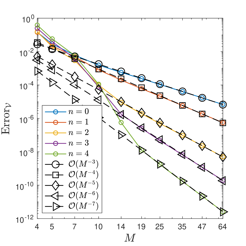
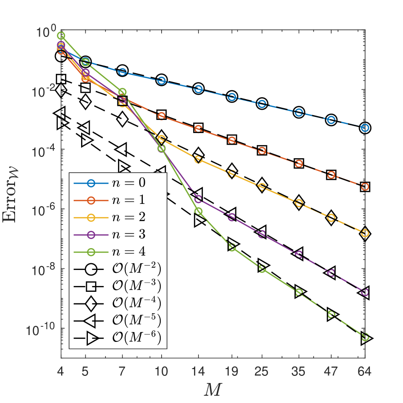
((a)) Disk

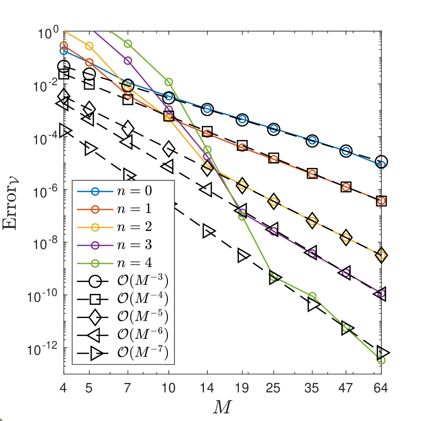
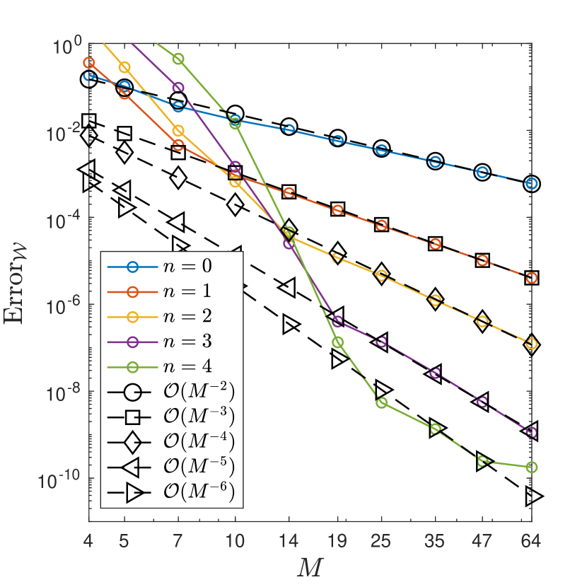
((b)) Kite

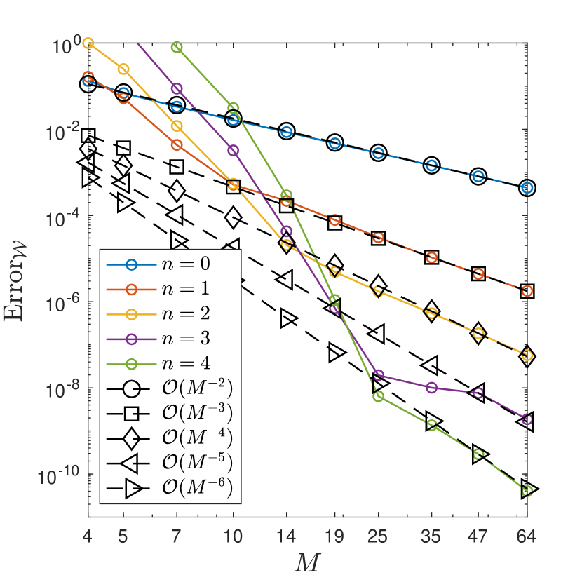
((c)) Jellyfish

Figure 4: Numerical accuracy in the numerical evaluation of the volume potentials $\mathcal{V}_{k}$ and $\mathcal{W}_{k}$ using Taylor density interpolation over quad-meshed domains. Top row: The three domains $\Omega$ whose curve parametrizations are given in Eq. 66, that are represented using mapped-quadrilateral patches. Middle and bottom rows: Relative errors in the numerical evaluation of $\mathcal{V}_{k}$ (middle row) and $\mathcal{W}_{k}$ (bottom row) for different discretization sizes.

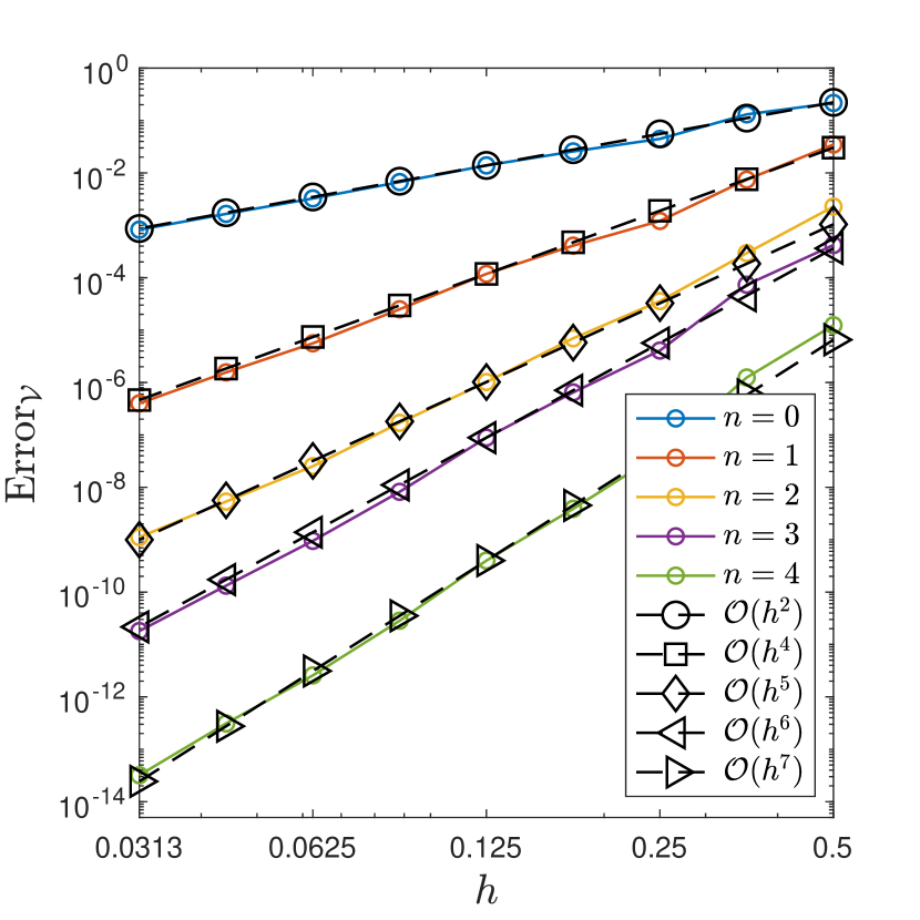
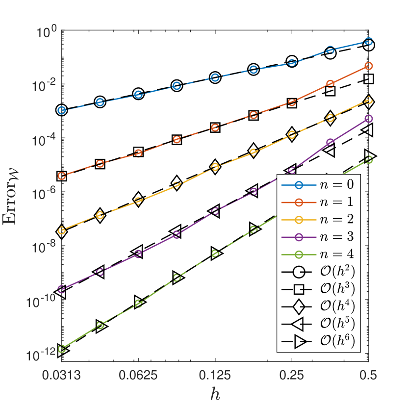
((a)) Disk

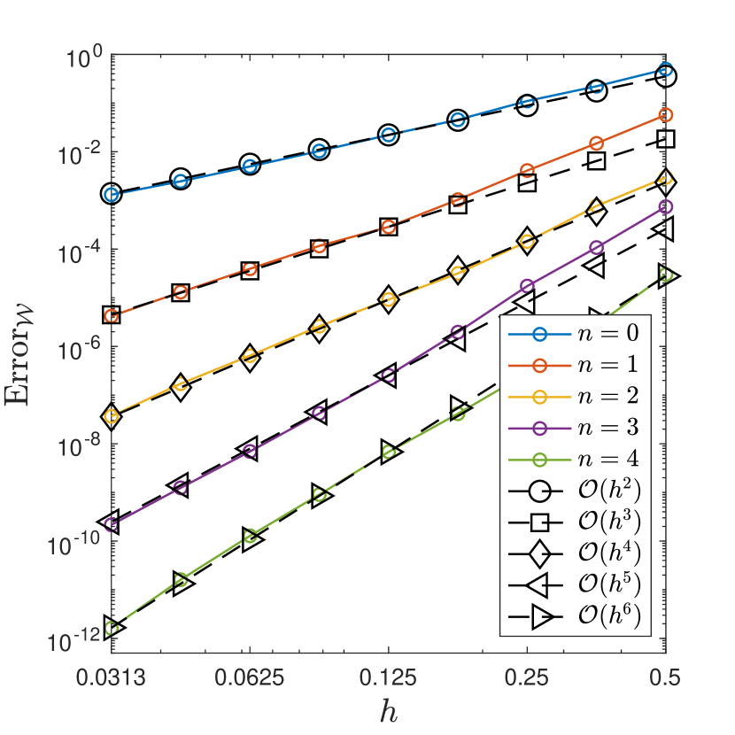
((b)) Kite

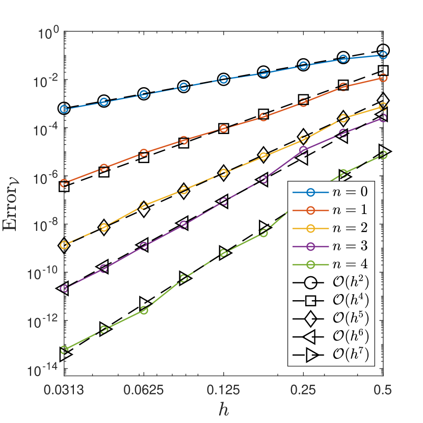
((c)) Jellyfish

Figure 5: Numerical accuracy in the evaluation of volume potentials $\mathcal{V}_{k}$ and $\mathcal{W}_{k}$ using Lagrange density interpolation over triangular-meshed domains. Top Row: Initial triangular meshes representing the three domains $\Omega$, with their respective curve parametrizations given in Eq. 66 and the Vioreanu-Rokhlin quadrature/interpolation nodes for $n=5$. Middle and Bottom Rows: Relative errors in the numerical evaluation of $\mathcal{V}_{k}$ (middle row) and $\mathcal{W}_{k}$ (bottom row) for various discretization sizes.

For the Taylor density interpolation method, which relies on a quad-based mesh of the domain and a tensor product Fejér’s quadrature rule, we maintain a constant number $L$ of mapped-quadrilateral domain patches that together form $\Omega$. In fact, discretization is a function of both $L$ and $M$, and experiments using an alternate strategy of subdividing patches (increasing $L$) while keeping $M$ fixed could be contemplated; we choose the present strategy, that can be viewed as isolating the effect of interpolation error dominating, as an illustrative point of contrast to the Lagrange case where in the simple case of Vioreanu-Rokhlin interpolation/quadrature the quadrature order is closely related to interpolation order. To experimentally determine the rate of convergence of the method, we then increase the number of quadrature nodes $N=LM^{2}$ by increasing $M$, the number of Fejér nodes in one dimension. The results of this example are shown in Figure 4. The top row of Figure 4 displays the fixed patches used for each of the domains considered, while the middle and bottom rows respectively display the relative errors ${\rm Error}_{\mathcal{V}}$ and $\rm Error_{\mathcal{W}}$ in Eq. 67 obtained for various values of the mesh parameter $M$. For the interpolation orders $n\in\{0,1,2,3,4\}$ considered in these examples, we observe that ${\rm Error}_{\mathcal{V}}$ scales as $\mathcal{O}(M^{-(n+3)})$ as $M$ increases while ${\rm Error}_{\mathcal{W}}$, in turn, scales as $\mathcal{O}(M^{-(n+2)})$. Note that these results are in accordance with the singularity degree of the integral kernels; the accuracy deteriorates as the singularity degree of the kernel increases. The general-purpose DIM [20] was utilized in all these examples to accurately evaluate the layer potentials ($\mathcal{B}_{\Gamma}$ in Table 1) that arise in both the regularization formula Eq. 8 and in the reference solution Eq. 64. In the former case, the boundary $\Gamma$ is decomposed into curved segments corresponding to the parts of the boundary $\Gamma$ contained in the domain’s patches that intercept the boundary. The layer potentials are then evaluated by integrating over each segment using, again, Fejér’s quadrature rule. The total number of boundary discretization points is kept proportional to $M\propto N^{1/2}$ where $N$ is the total number of volume quadrature nodes. This choice ensures that the accuracy of the layer potential evaluation also improves as the domain discretization is refined. In the latter case, on the other hand, we employ a further refined boundary discretization, achieved by doubling the number of Fejér nodes on each of the curved boundary segments, that ensures the attainment of significantly higher accuracy for the reference solutions $v_{\rm ref}$ and $w_{\rm ref}$.

A wide pre-asymptotic regime is observed for the higher-order versions of the Taylor density interpolation method considered in Figure 4, which perform worse than the lower-order ones over coarse grids (especially for the more complicated jellyfish domain). This phenomenon could be explained by the fact that as the interpolation order increases, so does the degree of the polynomials that have to be resolved by the fixed discretization grid. Coarser grids are not good enough to properly capture the growth and wild variations of the higher-degree polynomials over the curved surface patches, eventually leading to numerical errors that dominate over the singular-integration error targeted by our method. This suggests that for moderate accuracies ($\sim 10^{-3}$ relative errors) low order methods (i.e., $n\in\{0,1,2\}$) for the regularization are advantageous. Finally, our numerical experiments (unreported here) indicate the alternate strategy of keeping $M$ fixed while increasing $L$ via patch subdivision exhibits somewhat steadier convergence.

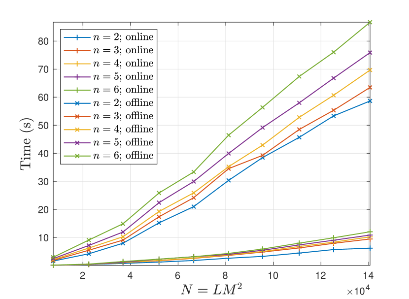
((a)) Quad-meshed kite-shaped domains comprising $L=9$ patches, each utilizing Chebyshev grids with $M\times M$ points.

((b)) Triangular-meshed kite-shaped domains consisting of $L$ triangles, with each triangle employing $q_{n}$ Vioreanu-Rokhlin quadrature/interpolation nodes.

Figure 6: Computation times (in seconds) for evaluating $\mathcal{V}_{k}[f]$ over progressively larger discretizations of the kite-shaped domain whose boundary $\boldsymbol{\gamma}_{2}$ is given in (66b). The two different density interpolation approaches, namely Taylor (left) and Lagrange (right), were employed in this example.

Next, we conduct a similar experiment, but this time, we employ the Lagrange density interpolation method, which utilizes (curved) triangular meshes and Vioreanu-Rokhlin quadrature nodes for integration and interpolation, as detailed in Section 3.2. The results are presented in Figure 5, showcasing the obtained errors, ${\rm Error}_{\mathcal{V}}$ and ${\rm Error}_{\mathcal{W}}$, for meshes of varying sizes $h$ and interpolation orders $n\in\{0,1,2,3,4\}$. Notably, we observe clear convergence orders for interpolation orders $n\in\{0,2,3,4\}$, that match the error estimates established in Theorem 3.11. However, interestingly, for the $\mathcal{V}_{k}$ operator, we observe evidence of super-convergence in the case $n=1$ even as the expected rate is observed for the $\mathcal{W}_{k}$ operator (see Remark 3.12).

Finally, in Figure 6, we showcase the timing results obtained from the numerical evaluation of the operator $\mathcal{V}_{k}$ over the kite-shaped domain using Taylor and Lagrange density interpolation for orders $n=\{0,1,2,3,4\}$ and for increasingly large discretizations. The implementation of this code in Matlab is unoptimized. To accelerate both volume and layer potential evaluations, we utilize the FMM as implemented in the fmm2d library (https://github.com/flatironinstitute/fmm2d). The plots displayed in the linear-linear scale exhibit excellent agreement with the asymptotic complexity estimates presented in Table 1, as they demonstrate that the overall cost of the algorithm scale linearithmically with the total number of discretization points $N$. Notably, the offline ($f$-independent) part of the algorithm incurs significantly higher costs compared to the online ($f$-dependent) part, despite the $\mathcal{O}(q_{n}^{2}N)$ cost associated with the interpolation of the density. This observation can be attributed to a constant factor that multiplies the $\mathcal{O}(q_{n}N\log N)$ cost of the FMM, which is significantly larger than the corresponding factor multiplying the $\mathcal{O}(q_{n}^{2}N)$ interpolation cost. Additionally, we note that when comparing the two approaches for roughly the same number of discretization points $N$, the Lagrange interpolation method appears to be relatively more expensive than the Taylor interpolation method. This discrepancy can be attributed to the code implementation in Matlab, where the Taylor density interpolation leverages vectorization more efficiently, resulting in improved performance.

4.2 Lippmann-Schwinger equation

To demonstrate the practical application of our proposed methodology, we employ it to solve the scattering problem of a planewave $u^{\rm inc}(\boldsymbol{x})=\exp(ik\boldsymbol{x}\cdot\boldsymbol{\theta})$, $|\boldsymbol{\theta}|=1$, interacting with a scatterer $\Omega\subset\mathbb{R}^{2}$ with the examples thus showing how the high-order accurate operator evaluation previously demonstrated can lead to a high-order volume integral equation solver. We consider a scatterer that has a smooth refractive index function $\nu>0$ defined within its boundaries. Outside of $\Omega$, we assume a constant refractive index of $\nu=1$. The scattering problem seeks a volumetric total field $u:\mathbb{R}^{2}\to\mathbb{C}$, $u\in C^{1}(\mathbb{R}^{2})\cap H^{2}_{\rm loc}(\mathbb{R}^{2})$, that satisfies the Helmholtz equation

(68) $$\Delta u+\nu(\boldsymbol{x})k^{2}u=0 \quad\text{in}\quad\mathbb{R}^{2}\setminus\Gamma,$$

with the scattered field $u^{\rm sc}\coloneqq u-u^{\rm inc}$ satisfying Sommerfeld’s radiation condition. It can also be reformulated as the Lippmann-Schwinger volume integral equation for $u$ inside the scatterer:

(69) $$u(\boldsymbol{x})+k^{2}\mathcal{V}_{k}\left[(1-\nu)u\right](\boldsymbol{x})=u^{\mathrm{inc}}(\boldsymbol{x}),\quad\boldsymbol{x}\in\Omega,$$

with the solution outside the scatterer given by the representation formula

(70) $$u(\boldsymbol{x})=u^{\mathrm{inc}}(\boldsymbol{x})-k^{2}\mathcal{V}_{k}[(1-\nu)u](\boldsymbol{x}),\quad\boldsymbol{x}\in\mathbb{R}^{2}\setminus\overline{\Omega}.$$

The Lippmann-Schwinger equation (69) can be effectively solved using Nyström methods based on the high-order discretization approaches presented above in Section 3 using iterative methods, wherein the resulting $N\times N$ linear system for the approximate values of the total field at the quadrature nodes $\{\boldsymbol{\xi}_{j}\}_{j=1}^{N}$ is solved via GMRES [47] and the volume integral operator $\mathcal{V}_{k}$ is used as a forward map. This methodology, which only necessitates repeated applications of the operator $\mathcal{V}_{k}$ over the fixed domain $\Omega$, allows us to exploit the algorithm’s potential fully, as all source-independent steps can be precomputed and reused at each operator application (see Table 1).

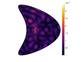
((a)) Planewave scattering by a homogeneous obstacle, for $k=2\pi$ and $\nu=4$ in $\Omega$. Left: Real part of the solution of the transmission problem (71). Middle and right: Absolute pointwise error in Lippmann-Schwinger equation solutions obtained using Taylor and Lagrange density interpolation-based Nyström methods, respectively.

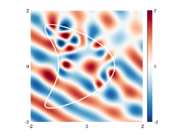
((b)) Planewave scattering by an inhomogeneous obstacle. Left: Piecewise smooth refractive index $\nu$. Middle and right: Real part of approximate Lippmann-Schwinger equation solutions obtained using Taylor and Lagrange density interpolation-based Nyström methods, respectively.

Figure 7: Application of the polynomial density interpolation method to the Lippmann-Schwinger equation. Convergence experiments demonstrate the same high convergence orders for solution of the volume integral equation that are illustrated for the operator evaluation in Figures 4 and 5, and to our knowledge represent the first reported high-order accurate solutions of such integral equations with piecewise-continuous material parameters.

To assess the accuracy of such a Nyström method for the Lippmann-Schwinger equation, we focus on a specific scenario where $\nu$ maintains a constant value of $4$ within $\Omega$. In this case, the total field can be determined by solving the transmission problem

(71) $$\Delta u+\nu k^{2}u=0\ \text{ in }\Omega, \qquad\Delta u^{\rm sc}+k^{2}u^{\rm sc}=0\ \text{ in }\mathbb{R}^{2}\setminus\overline{\Omega},$$

$$u=u^{\rm inc}+u^{\rm sc} \text{and}\quad\partial_{n}u=\partial_{n}\left(u^{\rm inc}+u^{\rm sc}\right)\text{ on }\Gamma.$$

that can itself be recast into a second-kind boundary integral equation [35]. By solving the boundary integral equation (and employing an exponentially convergent Nyström method, based on the Martensen-Kussmaul quadrature rule [15, Sec. 3.5] for kernels with logarithmic singularities to do so), we obtain a highly accurate reference solution that serves as the benchmark to quantify the error in the solution of the volume integral equation for this piecewise constant refractive index medium. Figure 7(a) displays the pointwise errors within $\Omega$ in the volume integral equation solutions obtained utilizing the Taylor (resp. Lagrange) density interpolation-based Nyström method for $n=3$ (resp. $n=4$) and $M=64$ (resp. $h=0.08$), which correspond to the same parameters utilized in the respective panels of Figure 7(b).

We consider, finally, a more interesting scattering problem involving a piecewise-smooth refractive index $\nu$, seen in the scatterer in the left panel of Figure 7(b). The remaining panels of that figure show the real part of the total field obtained by the two discretization methods considered in this work. GMRES convergence was achieved in these examples after about $80$ iterations for a relative error tolerance of $10^{-9}$ using $k=2\pi$ and $\boldsymbol{\theta}=(\cos\frac{\pi}{3},\sin\frac{\pi}{3})$.

5 Conclusions

We have presented a provably high-order scheme for the numerical evaluation of volume integral operators that is amenable to fast algorithms. Future work will consider macro forms of domain subdivision and their effect on computational efficiency. Applications to other PDEs will be explored in future work and is in some cases quite natural given the generality afforded by [20, 2]. The reduction in the dimensionality of the region of singular quadrature should prove especially effective in three dimensions. The implementation we presented here was rudimentary; we look forward to optimized and parallelized schemes built on these concepts and coupling them to more adaptive methods.

References

• [1] S. Ambikasaran, C. Borges, L.-M. Imbert-Gerard, and L. Greengard, Fast, adaptive, high-order accurate discretization of the Lippmann–Schwinger equation in two dimensions, SIAM Journal on Scientific Computing, 38 (2016), pp. A1770–A1787.
• [2] T. G. Anderson, M. Bonnet, L. M. Faria, and C. Pérez-Arancibia, On particular solutions of linear partial differential equations with polynomial right-hand-sides, arXiv preprint arXiv:2306.13628, (2023).
• [3] T. G. Anderson, H. Zhu, and S. Veerapaneni, A fast, high-order scheme for evaluating volume potentials on complex 2d geometries via area-to-line integral conversion and domain mappings, Journal of Computational Physics, 472 (2023), p. 111688.
• [4] K. E. Atkinson, The numerical evaluation of particular solutions for Poisson’s equation, IMA Journal of Numerical Analysis, 5 (1985), pp. 319–338, https://doi.org/10.1093/imanum/5.3.319.
• [5] K. E. Atkinson, The Numerical Solution of Integral Equations of the Second Kind, vol. 4, Cambridge university press, 1997.
• [6] A. Averbuch, E. Braverman, and M. Israeli, Parallel adaptive solution of a Poisson equation with multiwavelets, SIAM Journal on Scientific Computing, 22 (2000), pp. 1053–1086.
• [7] C. Bauinger and O. P. Bruno, “Interpolated factored Green function” method for accelerated solution of scattering problems, Journal of Computational Physics, 430 (2021), p. 110095.
• [8] S. Börm, L. Grasedyck, and W. Hackbusch, Introduction to hierarchical matrices with applications, Engineering Analysis with Boundary Elements, 27 (2003), pp. 405–422.
• [9] S. Börm and J. M. Melenk, Approximation of the high-frequency Helmholtz kernel by nested directional interpolation: error analysis, Numerische Mathematik, 137 (2017), pp. 1–34.
• [10] J. P. Boyd, Chebyshev and Fourier Spectral Methods, Courier Corporation, 2001.
• [11] O. P. Bruno and E. M. Hyde, An efficient, preconditioned, high-order solver for scattering by two-dimensional inhomogeneous media, Journal of Computational Physics, 200 (2004), pp. 670–694.
• [12] O. P. Bruno and A. Pandey, Fast, higher-order direct/iterative hybrid solver for scattering by inhomogeneous media–with application to high-frequency and discontinuous refractivity problems, arXiv preprint arXiv:1907.05914, (2019).
• [13] O. P. Bruno and J. Paul, Two-dimensional Fourier continuation and applications, SIAM Journal on Scientific Computing, 44 (2022), pp. A964–A992.
• [14] P. G. Ciarlet and P.-A. Raviart, General Lagrange and Hermite interpolation in $\mathbb{R}^{n}$ with applications to finite element methods, Archive for Rational Mechanics and Analysis, 46 (1972), pp. 177–199.
• [15] D. Colton and R. Kress, Inverse Acoustic and Electromagnetic Scattering Theory, vol. 93, Springer, third ed., 2012.
• [16] A. R. Conn, K. Scheinberg, and L. N. Vicente, Geometry of interpolation sets in derivative free optimization, Mathematical programming, 111 (2008), pp. 141–172.
• [17] T. Dangal, C.-S. Chen, and J. Lin, Polynomial particular solutions for solving elliptic partial differential equations, Computers & Mathematics with Applications, 73 (2017), pp. 60–70.
• [18] P. J. Davis and P. Rabinowitz, Methods of Numerical Integration, Courier Corporation, 2007.
• [19] F. Ethridge and L. Greengard, A new fast-multipole accelerated Poisson solver in two dimensions, SIAM Journal on Scientific Computing, 23 (2001), pp. 741–760.
• [20] L. M. Faria, C. Pérez-Arancibia, and M. Bonnet, General-purpose kernel regularization of boundary integral equations via density interpolation, Computer Methods in Applied Mechanics and Engineering, 378 (2021), p. 113703.
• [21] F. Fryklund and L. Greengard, An FMM accelerated poisson solver for complicated geometries in the plane using function extension, arXiv preprint arXiv:2211.14537, (2022).
• [22] F. Fryklund, E. Lehto, and A.-K. Tornberg, Partition of unity extension of functions on complex domains, Journal of Computational Physics, 375 (2018), pp. 57–79.
• [23] M. I. Ganzburg, A Markov-type inequality for multivariate polynomials on a convex body, Journal of Computational Analysis and Applications, 4 (2002), pp. 265–268.
• [24] M. Gasca and T. Sauer, Polynomial interpolation in several variables, Advances in Computational Mathematics, 12 (2000), pp. 377–410.
• [25] M. Golberg, A. Muleshkov, C. Chen, and A.-D. Cheng, Polynomial particular solutions for certain partial differential operators, Numerical Methods for Partial Differential Equations: An International Journal, 19 (2003), pp. 112–133.
• [26] V. Gómez and C. Pérez-Arancibia, On the regularization of Cauchy-type integral operators via the density interpolation method and applications, Computers & Mathematics with Applications, 87 (2021), pp. 107–119.
• [27] W. J. Gordon and C. A. Hall, Construction of curvilinear co-ordinate systems and applications to mesh generation, International Journal for Numerical Methods in Engineering, 7 (1973), pp. 461–477.
• [28] W. J. Gordon and C. A. Hall, Transfinite element methods: blending-function interpolation over arbitrary curved element domains, Numerische Mathematik, 21 (1973), pp. 109–129.
• [29] L. Greengard and J.-Y. Lee, A direct adaptive Poisson solver of arbitrary order accuracy, Journal of Computational Physics, 125 (1996), pp. 415–424.
• [30] L. Greengard and V. Rokhlin, A fast algorithm for particle simulations, Journal of Computational Physics, 73 (1987), pp. 325–348.
• [31] E. Isaacson and H. B. Keller, Analysis of numerical methods, New York: Wiley, (1966).
• [32] M. Israeli, E. Braverman, and A. Averbuch, A hierarchical 3-D Poisson modified Fourier solver by domain decomposition, Journal of Scientific Computing, 17 (2002), pp. 471–479.
• [33] P. Knupp and S. Steinberg, Fundamentals of Grid Generation, CRC press, 2020.
• [34] D. Kopriva et al., High Order Hex-Quad Mesher. https://github.com/trixi-framework/HOHQMesh.
• [35] R. Kress and G. Roach, Transmission problems for the Helmholtz equation, Journal of Mathematical Physics, 19 (1978), pp. 1433–1437.
• [36] W. Liu, L.-L. Wang, and H. Li, Optimal error estimates for Chebyshev approximations of functions with limited regularity in fractional sobolev-type spaces, Mathematics of Computation, 88 (2019), pp. 2857–2895.
• [37] J. Lyness, An error functional expansion for 2-dimensional quadrature with an integrand function singular at a point, Mathematics of Computation, 30 (1976), pp. 1–23.
• [38] P. A. Martin, Acoustic scattering by inhomogeneous obstacles, SIAM Journal on Applied Mathematics, 64 (2003), pp. 297–308.
• [39] L. Matthys, H. Lambert, and G. De Mey, A recursive construction of particular solutions to a system of coupled linear partial differential equations with polynomial source term, Journal of Computational and Applied Mathematics, 69 (1996), pp. 319–329.
• [40] P. McCorquodale, P. Colella, G. Balls, and S. Baden, A local corrections algorithm for solving Poisson’s equation in three dimensions, Communications in Applied Mathematics and Computational Science, 2 (2007), pp. 57–81.
• [41] D. Nardini and C. Brebbia, A new approach to free vibration analysis using boundary elements, Applied Mathematical Modelling, 7 (1983), pp. 157–162.
• [42] P. J. Olver, On multivariate interpolation, Studies in Applied Mathematics, 116 (2006), pp. 201–240.
• [43] P. W. Partridge and C. A. Brebbia, Dual reciprocity boundary element method, Springer Science & Business Media, 2012.
• [44] C. Pérez-Arancibia, A plane-wave singularity subtraction technique for the classical Dirichlet and Neumann combined field integral equations, Applied Numerical Mathematics, 123 (2018), pp. 221–240.
• [45] C. Pérez-Arancibia, L. M. Faria, and C. Turc, Harmonic density interpolation methods for high-order evaluation of Laplace layer potentials in 2D and 3D, Journal of Computational Physics, 376 (2019), pp. 411–434.
• [46] C. Pérez-Arancibia, C. Turc, and L. Faria, Planewave density interpolation methods for 3D Helmholtz boundary integral equations, SIAM Journal on Scientific Computing, 41 (2019), pp. A2088–A2116.
• [47] Y. Saad and M. H. Schultz, GMRES: A generalized minimal residual algorithm for solving nonsymmetric linear systems, SIAM Journal on Scientific and Statistical Computing, 7 (1986), pp. 856–869.
• [48] J. Saranen and G. Vainikko, Periodic integral and pseudodifferential equations with numerical approximation, Springer Science & Business Media, 2001.
• [49] T. Sauer and Y. Xu, On multivariate Lagrange interpolation, Mathematics of computation, 64 (1995), pp. 1147–1170.
• [50] S. A. Sauter and C. Schwab, Boundary Element Methods, Springer, 2010.
• [51] Z. Shen and K. Serkh, Rapid evaluation of Newtonian potentials on planar domains, arXiv preprint arXiv:2208.10443, (2022).
• [52] D. B. Stein, Spectrally accurate solutions to inhomogeneous elliptic PDE in smooth geometries using function intension, arXiv preprint arXiv:2203.01798, (2022).
• [53] D. B. Stein, R. D. Guy, and B. Thomases, Immersed boundary smooth extension: a high-order method for solving PDE on arbitrary smooth domains using Fourier spectral methods, Journal of Computational Physics, 304 (2016), pp. 252–274.
• [54] G. Strang, Approximation in the finite element method, Numerische Mathematik, 19 (1972), pp. 81–98.
• [55] L. N. Trefethen, Approximation Theory and Approximation Practice, Extended Edition, SIAM, 2019.
• [56] G. Vainikko, Multidimensional Weakly Singular Integral Equations, Springer, 2006.
• [57] B. Vioreanu and V. Rokhlin, Spectra of multiplication operators as a numerical tool, SIAM Journal on Scientific Computing, 36 (2014), pp. A267–A288.
• [58] H. Xiao and Z. Gimbutas, A numerical algorithm for the construction of efficient quadrature rules in two and higher dimensions, Computers & mathematics with applications, 59 (2010), pp. 663–676.