FADE: Enabling Federated Adversarial Training
on Heterogeneous Resource-Constrained Edge Devices

Abstract

Federated adversarial training can effectively complement adversarial robustness into the privacy-preserving federated learning systems. However, the high demand for memory capacity and computing power makes large-scale federated adversarial training infeasible on resource-constrained edge devices. Few previous studies in federated adversarial training have tried to tackle both memory and computational constraints simultaneously. In this paper, we propose a new framework named Federated Adversarial Decoupled Learning (FADE) to enable AT on heterogeneous resource-constrained edge devices. FADE differentially decouples the entire model into small modules to fit into the resource budget of each device, and each device only needs to perform AT on a single module in each communication round. We also propose an auxiliary weight decay to alleviate objective inconsistency and achieve better accuracy-robustness balance in FADE. FADE offers theoretical guarantees for convergence and adversarial robustness, and our experimental results show that FADE can significantly reduce the consumption of memory and computing power while maintaining accuracy and robustness.

1 Introduction

As a privacy-preserving distributed learning paradigm, Federated Learning (FL) makes a meaningful step toward the practice of secure and trustworthy artificial intelligence (Konečnỳ et al., 2015, 2016; McMahan et al., 2017; Kairouz et al., 2019). In contrast to traditional centralized training, FL pushes the training to edge devices (clients), and client models are locally trained and uploaded to the server for aggregation. Since no private data is shared with other clients or the server, FL substantially improves data privacy during the training process.

While FL can preserve the privacy of the participants, other threats can still impact the reliability of the machine learning model running on the FL system. One such threat is adversarial examples that aim to cause misclassifications by adding imperceptible noise into the input data (Szegedy et al., 2013; Goodfellow et al., 2014). Previous research has shown that performing adversarial training (AT) on a large model is an effective method to attain robustness against adversarial examples while maintaining high accuracy on clean data (Liu et al., 2020). However, large-scale AT also puts high demand for both memory capacity and computing power. Thus it becomes unaffordable for some edge devices with limited resources, such as mobile phones and IoT devices that contribute to the majority of the participants in cross-device FL (Kairouz et al., 2019; Li et al., 2020; Wong et al., 2020; Zizzo et al., 2020; Hong et al., 2021). Table 1 shows that strong robustness of the whole FL system cannot be attained by allowing only a small portion (e.g., $20\%$) of the clients to perform AT. Therefore, enabling resource-constrained edge devices to perform AT is necessary for achieving strong robustness in FL.

Table 1: Results of partial federated adversarial training with 100 clients. “$20\%$ AT + $80\%$ ST” means that $20\%$ clients perform AT while $80\%$ clients perform standard training (ST).

Training Scheme	FMNIST (CNN-7)		CIFAR-10 (VGG-11)
	Natural Acc.	Adversarial Acc.	Natural Acc.	Adversarial Acc.
$100\%$ AT + $0\%$ ST	$78.39\%$	$66.93\%$	$64.73\%$	$33.27\%$
$20\%$ AT + $80\%$ ST	$83.83\%$	$48.61\%$	$74.77\%$	$19.22\%$

Some previous works have tried to tackle client-wise systematic heterogeneity in FL (Li et al., 2018; Xie et al., 2019; Lu et al., 2020; Wang et al., 2020b). The most common method is allowing slow devices to perform fewer epochs of local training than the others (Li et al., 2018; Wang et al., 2020b). While this method can reduce the computational costs on resource-constrained devices, the memory capacity limitation has not been well addressed in these works.

To tackle both memory capacity and computing power constraints, recent studies propose a novel training scheme named Decoupled Greedy Learning (DGL) which partitions the entire neural network into multiple small modules and trains each module separately (Belilovsky et al., 2019; Wang et al., 2021). Although DGL successfully reduces both memory and computational requirements for training large models, the exploration and convergence analysis of DGL are limited to the case that all computing nodes adopt the same partition of the model (Belilovsky et al., 2020), which cannot fit into different resource budgets of different clients in heterogeneous FL. Additionally, no previous studies have discussed whether DGL can be combined with AT to confer joint adversarial robustness to the entire model. It is not trivial to achieve joint robustness of the entire model when applying AT with DGL, since DGL trains each module separately with different locally supervised losses.

In this paper, we propose Federated Adversarial DEcoupled Learning (FADE), which is the first adversarial decoupled learning framework for heterogeneous FL with convergence and robustness guarantees. Our main contributions are:

1. We propose Federated Decoupled Learning (FDL) allowing differentiated model partitions on heterogeneous devices with different resource budgets. We give a theoretical guarantee for the convergence of FDL.

2. We propose Federated Adversarial DEcoupled Learning (FADE) to attain theoretically guaranteed joint adversarial robustness of the entire model. Our experimental results show that FADE can significantly reduce the memory and computational requirements while maintaining almost the same natural accuracy and adversarial robustness as joint training.

3. We reveal the non-trivial relationship between objective consistency (natural accuracy) and adversarial robustness in FADE, and we propose an effective method to achieve a better accuracy-robustness balance point with the weight decay on auxiliary models.

2 Preliminary

Federated Learning (FL)

In FL, different clients collaboratively train a shared global model ${\bm{w}}$ with locally stored data (McMahan et al., 2017). The objective of FL is:

$$\min_{{\bm{w}}} \quad L({\bm{w}})=\sum_{k=1}^{N}q_{k}L_{k}({\bm{w}}),$$ (1)

where $$\quad L_{k}({\bm{w}})=\frac{1}{|{\mathbb{D}}_{k}|}\sum_{({\bm{x}},y)\in{\mathbb{D}}_{k}}l({\bm{x}},y;{\bm{w}}),$$ (2)

and $l$ is the task loss, e.g., cross-entropy loss for classification tasks. ${\mathbb{D}}_{k}$ is the dataset of client $k$ and its weight $q_{k}=|{\mathbb{D}}_{k}|/(\sum_{i}|{\mathbb{D}}_{i}|)$. To solve for the optimal solution of this objective, in each communication round, FL first samples a subset of clients ${\mathbb{S}}^{(t)}$ to perform local training. These clients initialize their models with the global model ${\bm{w}}_{k}^{(t,0)}={\bm{w}}^{(t)}$, and then run $\tau$ iterations of local SGD. After all these clients complete training in this round, their models are uploaded and averaged to become the new global model (McMahan et al., 2017). We summarize this procedure as follows:

$${\bm{w}}_{k}^{(t+1)} ={\bm{w}}^{(t)}-\eta_{t}\sum_{j=0}^{\tau-1}\nabla L_{k}({\bm{w}}_{k}^{(t,j)}),$$ (3)

$${\bm{w}}^{(t+1)} =\frac{1}{\sum_{i\in{\mathbb{S}}^{(t)}}q_{i}}\sum_{k\in{\mathbb{S}}^{(t)}}q_{k}{\bm{w}}_{k}^{(t+1)},$$ (4)

where ${\bm{w}}_{k}^{(t,j)}$ is the local model of client $k$ at the $j$-th iteration of communication round $t$.

Adversarial Training (AT)

The goal of AT is to achieve robustness against small perturbations in the inputs. We define $(\epsilon,c)$-robustness as follows:

Definition 2.1.

We say a model ${\bm{w}}$ is $(\epsilon,c)$-robust in a loss function $l$ at input ${\bm{x}}$ if $\forall\bm{\delta}\in\{\bm{\delta}:\|\bm{\delta}\|_{p}\leq\epsilon\}$,

$$l({\bm{x}}+\bm{\delta},y;{\bm{w}})-l({\bm{x}},y;{\bm{w}})\leq c,$$ (5)

where $\|\cdot\|_{p}$ is the $\ell_{p}$ norm of a vector, and $\epsilon$ is the perturbation tolerance.

AT trains a model with adversarial examples to achieve adversarial robustness, which can be formulated as a min-max problem (Goodfellow et al., 2014; Madry et al., 2017):

$$\min_{{\bm{w}}}\max_{\bm{\delta}:\|\bm{\delta}\|_{p}\leq\epsilon}l({\bm{x}}+\bm{\delta},y;{\bm{w}}).$$ (6)

To solve Equation 6, people usually alternatively solve the inner maximization and the outer minimization. While solving the inner maximization, Projected Gradient Descent (PGD) is shown to introduce the strongest robustness in AT (Madry et al., 2017; Wong et al., 2020; Wang et al., 2021).

Decoupled Greedy Learning (DGL)

The key idea of DGL is to partition the entire model into multiple non-overlapping small modules. By introducing a locally supervised loss to each module, we can load and train each module independently without accessing the other parts of the entire model (Belilovsky et al., 2019, 2020). This enables devices with small memory to train large models.

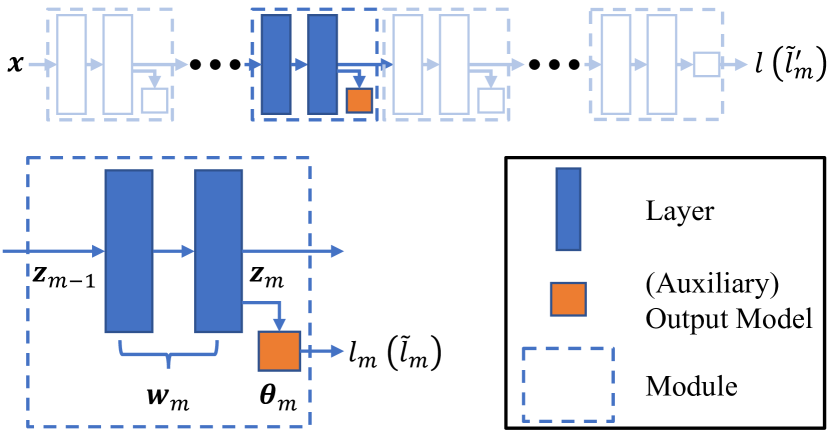
Figure 1: An illustration of DGL and a single module $m$.

As shown in Figure 1, each module $m$ contains one or multiple adjacent layers ${\bm{w}}_{m}$ of the backbone neural network, together with a small auxiliary model $\bm{\theta}_{m}$ that provides locally supervised loss. We denote $\bm{\Theta}_{m}=[{\bm{w}}_{m},\bm{\theta}_{m}]$ to be all the parameters in module $m$. Module $m$ accepts the features ${\bm{z}}_{m-1}$ from the previous module as the input, and it outputs features ${\bm{z}}_{m}=f_{m}({\bm{z}}_{m-1};{\bm{w}}_{m})$ for the following modules, as well as a locally supervised loss $l_{m}({\bm{z}}_{m-1},y;\bm{\Theta}_{m})$. At epoch $t$, the averaged locally supervised loss $L_{m}^{(t)}$ will be used for training this module:

$$L_{m}^{(t)}(\bm{\Theta}_{m}^{(t)})=\mathbb{E}_{({\bm{z}}_{m-1}^{(t)},y)}\left[l_{m}({\bm{z}}_{m-1}^{(t)},y;\bm{\Theta}_{m}^{(t)})\right].$$ (7)

In contrast to joint training, the input of one module can be various in different epochs in DGL since we may keep updating the previous modules during training. Thus we use ${\bm{z}}_{m-1}^{(t)}$ to denote the inputs of module $m$ in epoch $t$, and only the input of the first module ${\bm{z}}_{0}^{(t)}={\bm{x}}$ is invariant.

For convenience, we define the loss function of the auxiliary model $\bm{\theta}_{m}$ and the loss function of the following layers $[{\bm{w}}_{m+1},\cdots,{\bm{w}}_{M}]$ in the backbone network as

$$\tilde{l}_{m}({\bm{z}}_{m},y;\bm{\theta}_{m})=l_{m}({\bm{z}}_{m-1},y;\bm{\Theta}_{m}),$$ (8)

$$\tilde{l}^{\prime}_{m}({\bm{z}}_{m},y;{\bm{w}}_{m+1},\cdots,{\bm{w}}_{M})=l({\bm{x}},y;{\bm{w}}),$$ (9)

for each module $m$. Without specifying, we will omit all parameters (${\bm{w}}_{m},\bm{\theta}_{m}$ and $\bm{\Theta}_{m}$) in the following sections.

3 Federated Adversarial Decoupled Learning

In this section, we present Federated Adversarial Decoupled Learning (FADE), which aims at enabling all clients with different computing resources to participate in adversarial training. In Section 3.1, we introduce Federated Decoupled Learning (FDL) with differentiated model partitions for heterogeneous resource-constrained devices, and we analyze its convergence property. In Section 3.2, we integrate AT into FDL to achieve guaranteed joint adversarial robustness of the entire model. In Section 3.3, we discuss the objective inconsistency in FDL and propose an effective method to attain a better accuracy-robustness balance point.

3.1 Federated Decoupled Learning

In cross-device FL, the main participants are usually small edge devices that have limited hardware resources and may not be able to afford large-scale AT that requires large memory and high computing power (Li et al., 2018; Kairouz et al., 2019; Li et al., 2020; Wang et al., 2020b). A solution to tackle the resource constraints on edge devices is to deploy DGL in FL, such that each device only needs to load and train a single small module instead of the entire model in each communication round. However, DGL only allows a unified model partition on all the devices (Belilovsky et al., 2020). Considering the systematic heterogeneity, we would prefer differentiated model partitions to fit into different resource budgets of different clients. As shown in Figure 2, devices with limited resources (such as IoT devices) can partition the entire model into smaller modules, and devices with more resources (such as mobile phones or computers) can train larger modules or even the entire model.

Accordingly, we propose Federated Decoupled Learning (FDL) to tackle heterogeneous resource budgets. We define the model partition ${\mathbb{M}}_{k}$ as the set of all modules on client $k$. In contrast to DGL, since various model partitions ${\mathbb{M}}_{k}$ can be used by different clients in FDL, a module on one client may not be a module on the other clients. Thus instead of a specific module, we consider the aggregation rule of each layer $n$ with parameter $\bm{\omega}_{n}$ (either in the backbone network or in the auxiliary models), as one single layer is the “atom” in FDL and cannot be further partitioned. We use $m_{k}(n)$ to denote the module that contains layer $n$ on client $k$, and we define $L_{n,k}=L_{m_{k}(n),k}$ as the locally supervised loss for training this layer. In each communication round $t$, each client $k$ randomly samples a module $m_{k}^{t}$ from ${\mathbb{M}}_{k}$ for training (Equation 10). After the local training, the server averages the updates of each layer $n$ over clients whose trained modules contain layer $n$ in this round, i.e., clients in ${\mathbb{S}}_{n}^{(t)}=\{k\in{\mathbb{S}}^{(t)}:n\in m_{k}^{t}\}$ (Equation 11).

$$\bm{\omega}_{n,k}^{(t+1)}=\begin{cases}\bm{\omega}_{n}^{(t)}-\eta_{t}\sum_{j}\nabla_{\bm{\omega}_{n}}L_{n,k}^{(t)},\ \text{ if }n\in m_{k}^{t};\\ \bm{\omega}_{n}^{(t)},\qquad\qquad\qquad\qquad\ \text{elsewhere}.\end{cases}$$ (10)

$$\bm{\omega}_{n}^{(t+1)}=\frac{1}{\sum_{i\in{\mathbb{S}}_{n}^{(t)}}q_{i}}\sum_{k\in{\mathbb{S}}_{n}^{(t)}}q_{k}\bm{\omega}_{n,k}^{(t+1)}.$$ (11)

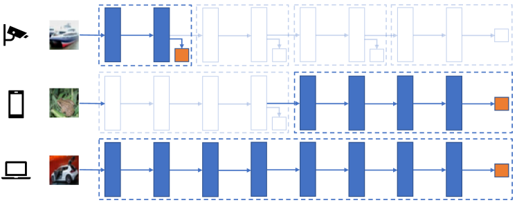
Figure 2: A framework of Federated Decoupled Learning. In contrast to using one unified partition in DGL (Belilovsky et al., 2020), we allow different model partitions among devices according to their resource budgets. In each communication round, each device randomly selects one module (highlighted) for training, and then the updates of each layer will be averaged respectively (column-wise in the figure).

Theorem 3.1 guarantees the convergence of FDL, while the full version with proof is given in Appendix A.

Theorem 3.1.

Under some common assumptions, the locally supervised loss $L_{n}=\sum_{k}q_{k}L_{n,k}$ of any layer $n$ can converge in Federated Decoupled Learning:

$$\lim_{T\rightarrow\infty}\inf_{t\leq T}\mathbb{E}\left\|\nabla_{\bm{\omega}_{n}}L_{n}\right\|^{2}=0.$$ (12)

Theorem 3.1 can guarantee the convergence of locally supervised loss $L_{n}$. However, because of the objective inconsistency $\|\nabla L-\nabla L_{n}\|\geq 0$, we cannot guarantee the convergence of the joint loss $L$ with this result. We will discuss the objective inconsistency in Section 3.3, and we will show how we can reduce this gap such that we can make the joint loss gradient $\nabla L$ smaller when the locally supervised loss $L_{n}$ converges.

3.2 Adversarial Decoupled Learning

Now we discuss how to integrate AT into FDL for joint robustness of the entire model. We consider the training on a single client in this section and the next, thus we omit client $k$ and use module $m$ instead of layer $n$ in the subscripts.

We can obtain adversarial decoupled learning by replacing the standard locally supervised loss of each module $m$ with the adversarial loss as follows:

$$\min_{\bm{\Theta}_{m}}\max_{\|\bm{\delta}_{m-1}\|\leq\epsilon_{m-1}}\quad l_{m}({\bm{z}}_{m-1}+\bm{\delta}_{m-1},y;\bm{\Theta}_{m}).$$ (13)

However, two concerns have not been addressed in adversarial decoupled learning:

1. Since different modules are trained with different locally supervised losses, can the local robustness in $l_{m}$ of each module guarantee the joint robustness in $l$ of the entire (backbone) model?

2. When applying AT on a module $m$, what value of the perturbation tolerance $\epsilon_{m-1}$ should we use to ensure the joint robustness of the entire model?

Theorem 3.2 reveals the relationship between the local robustness of each module and the joint robustness of the entire model, and it gives a lower bound of the perturbation tolerance $\epsilon_{m-1}$ for each module $m$ to sufficiently guarantee the joint robustness. Theorem 3.2 is proved in Section B.1.

Theorem 3.2.

Assume that $\tilde{l}_{m}({\bm{z}}_{m},y)$ is $\mu_{m}$-strongly convex in ${\bm{z}}_{m}$ for each module $m$. We can guarantee that the entire model has a joint $(\epsilon_{0},c_{M})$-robustness in $l({\bm{x}},y)$, if each module $m\leq M$ has local $(\epsilon_{m-1},c_{m})$-robustness in $l_{m}({\bm{z}}_{m-1},y)$, and

$$\quad\epsilon_{m}\geq\frac{g_{m}}{\mu_{m}}+\sqrt{\frac{2c_{m}}{\mu_{m}}+\frac{g_{m}^{2}}{\mu_{m}^{2}}},$$ (14)

where $g_{m}=\left\|\nabla_{{\bm{z}}_{m}}\tilde{l}_{m}({\bm{z}}_{m},y)\right\|$.

Remark 3.3.

In Theorem 3.2, we assume that the loss function $\tilde{l}_{m}({\bm{z}}_{m},y)$ of the auxiliary model $\bm{\theta}_{m}$ is strongly convex in its input ${\bm{z}}_{m}$. This assumption is realistic since the auxiliary model $\bm{\theta}_{m}$ is usually a very simple model, e.g., only a linear layer followed by cross-entropy loss. We also theoretically analyze the sufficiency of a simple auxiliary model in Section 3.3 (See Remark 3.5).

Theorem 3.2 shows that larger $\mu_{m}$ and smaller $g_{m}$ will lead to stronger joint robustness of the entire model since the lower bound of $\epsilon_{m}$ becomes smaller for ensuring the joint robustness. Both $\mu_{m}$ and $g_{m}$ are related to $\tilde{l}_{m}$ parameterized by the auxiliary model $\bm{\theta}_{m}$. We will discuss how we can regularize the auxiliary model to attain better robustness while reducing the objective inconsistency of FDL in Section 3.3.

3.3 Auxiliary Weight Decay

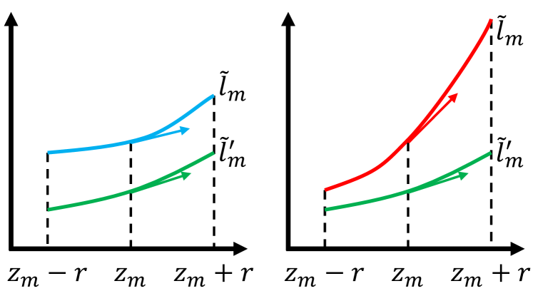
Figure 3: An illustration of the relationship between objective consistency and robustness. If both $\tilde{l}_{m}$ and $\tilde{l}_{m}^{\prime}$ are robust and smooth as shown in the left figure, their gradients are both close to $\bm{0}$ and the difference between the gradients is small. If $\tilde{l}_{m}$ is not robust, the difference between gradients is large in the right figure.

As we mentioned in Section 3.1, there exists objective inconsistency in FDL because each module is trained with the locally supervised loss instead of the joint loss. The objective inconsistency is defined as $\|\nabla_{{\bm{w}}_{m}}l-\nabla_{{\bm{w}}_{m}}l_{m}\|$, which is the difference between the gradients of the joint loss and the locally supervised loss. The existence of this inconsistency makes the optimal parameters that minimize the locally supervised loss $l_{m}$ not necessarily minimize the joint loss $l$. Furthermore, the objective inconsistency can enlarge heterogeneity among clients and hinder the convergence of FL (Li et al., 2019; Wang et al., 2020b). Therefore, it is important to alleviate the objective inconsistency in FDL to improve its convergence and performance.

Lemma 3.4 shows a non-trivial relationship between objective inconsistency and adversarial robustness: strong joint adversarial robustness also implies small objective inconsistency in FDL. We prove Lemma 3.4 in Section B.2.

Lemma 3.4.

Assume that $\tilde{l}_{m}({\bm{z}}_{m},y)$ and $\tilde{l}^{\prime}_{m}({\bm{z}}_{m},y)$ are $\beta_{m},\beta^{\prime}_{m}$-smooth in ${\bm{z}}_{m}$ for a module $m$. If there exist $\tilde{c}_{m}$, $\tilde{c}^{\prime}_{m}$, and $r\geq\sqrt{2\frac{\tilde{c}_{m}+\tilde{c}^{\prime}_{m}}{\beta_{m}+\beta^{\prime}_{m}}}$, such that the auxiliary model has $(r,\tilde{c}_{m})$-robustness in $\tilde{l}_{m}({\bm{z}}_{m},y)$, and the backbone network has $(r,\tilde{c}^{\prime}_{m})$-robustness in $\tilde{l}^{\prime}_{m}({\bm{z}}_{m},y)$, then we have:

$$\|\nabla_{{\bm{w}}_{m}}l- \nabla_{{\bm{w}}_{m}}l_{m}\|\leq\left\|\frac{\partial{\bm{z}}_{m}}{\partial{\bm{w}}_{m}}\right\|\|\nabla_{{\bm{z}}_{m}}\tilde{l}_{m}^{\prime}-\nabla_{{\bm{z}}_{m}}\tilde{l}_{m}\|$$

$$\leq \left\|\frac{\partial{\bm{z}}_{m}}{\partial{\bm{w}}_{m}}\right\|\sqrt{2(\tilde{c}_{m}+\tilde{c}^{\prime}_{m})(\beta_{m}+\beta^{\prime}_{m})}.$$ (15)

Lemma 3.4 suggests that we can alleviate the objective inconsistency by reducing $\beta_{m},\beta^{\prime}_{m},\tilde{c}_{m}$ and $\tilde{c}_{m}^{\prime}$ (Regularizing $\|\partial{\bm{z}}_{m}/\partial{\bm{w}}_{m}\|$ usually requires second derivative, which introduces high memory and computational overhead, so we do not consider it here). Notice that adversarial decoupled learning can guarantee an ($\epsilon_{m},c_{M}$)-robustness in $\tilde{l}^{\prime}_{m}$ according to Theorem 3.2, which implies a small $\tilde{c}_{m}^{\prime}$. Furthermore, Moosavi-Dezfooli et al. (2019) shows that adversarial robustness also implies a smoother loss function. Therefore, adversarial decoupled learning also leads to a small $\beta^{\prime}_{m}$.

Accordingly, with adversarial decoupled learning, reducing $\beta_{m}$ and $\tilde{c}_{m}$ can effectively alleviate the objective inconsistency, which is also illustrated in Figure 3. We notice that both $\beta_{m}$ and $\tilde{c}_{m}$ are only related to $\tilde{l}_{m}$ parameterized by the auxiliary model $\bm{\theta}_{m}$, and Section B.3 shows that we can reduce $\beta_{m}$ and $\tilde{c}_{m}$ by adding a large weight decay on the auxiliary model when it is simple (e.g., only a linear layer).

Remark 3.5.

It is noteworthy that we do not use any conditions on the difference between $\tilde{l}^{\prime}_{m}$ and $\tilde{l}_{m}$ in both Theorem 3.2 and Lemma 3.4 (also Figure 3). This implies that the auxiliary model is not required to perform as well as the joint backbone model. Thus, a simple auxiliary model is sufficient to achieve high joint robustness and low objective inconsistency in adversarial decoupled learning.

Based on all analysis in this work, we propose Federated Adversarial Decoupled Learning (FADE), where we replace the original loss function $l_{m}$ used by FDL with the following adversarial loss with weight decay on the auxiliary model:

$$l_{m}^{\text{FADE}}({\bm{z}}_{m-1}^{(t)},y;{\bm{w}}_{m}^{(t)},\bm{\theta}_{m}^{(t)})$$ (16)

$$= \max_{\bm{\delta}_{m-1}^{(t)}}\left[l_{m}({\bm{z}}_{m-1}^{(t)}+\bm{\delta}_{m-1}^{(t)},y;{\bm{w}}_{m}^{(t)},\bm{\theta}_{m}^{(t)})\right]+\lambda_{m}\|\bm{\theta}_{m}^{(t)}\|^{2},$$

where $\lambda_{m}$ is the hyperparameter that controls the weight decay on the auxiliary model $\bm{\theta}_{m}$. Our framework is summarized in Algorithm 1.

Algorithm 1 Federated Adversarial Decoupled Learning

1:  Initialize ${\bm{w}}^{(0)}$ and $\bm{\theta}_{m}^{(0)}$ for each module $m$.

2:  for $t=1,2,\cdots,T$ do

3:     Randomly sample a group of clients ${\mathbb{S}}^{(t)}$ for training.

4:     for each client $k\in{\mathbb{S}}^{(t)}$ in parallel do

5:        Randomly selects a module $m_{k}^{t}$.

6:        Download $\bm{\Theta}_{m_{k}^{t}}^{(t)}=[{\bm{w}}_{m_{k}^{t}}^{(t)},\bm{\theta}_{m_{k}^{t}}^{(t)}]$ from the server.

7:        Generate input features ${\bm{z}}_{m_{k}^{t}-1}^{(t)}$ for module $m_{k}^{t}$.

8:        Perform AT on module $m_{k}^{t}$ with $l_{m_{k}^{t}}^{\text{FADE}}$ in Equation 16 for $\tau$ iterations, and get $\bm{\Theta}_{m_{k}^{t},k}^{(t+1)}$.

9:        Upload $\bm{\Theta}_{m_{k}^{t},k}^{(t+1)}$ to the server.

10:     end for

11:     The server aggregates $\bm{\omega}_{n,k}^{(t+1)}$ to get $\bm{\omega}_{n}^{(t+1)}$ according to Equation 11 for each layer $n$.

12:  end for

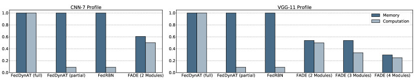
Figure 4: Minimum memory and computational requirements of baselines and FADE with different numbers of modules. The results are shown as the percentage of the resource requirement of full FedDynAT with PGD-10 AT.

Trade-off Between Joint Accuracy and Joint Robustness.

As we discussed in Section 3.2 and this section, four parameters ($\mu_{m},g_{m},\tilde{c}_{m}$ and $\beta_{m}$) that are only related to the auxiliary model $\bm{\theta}_{m}$ can influence the joint robustness and objective consistency. We can see in Section B.3 that applying a larger $\lambda_{m}$ can decrease all of them. Smaller $\tilde{c}_{m}$ and $\beta_{m}$ can alleviate the objective inconsistency to increase the joint accuracy, and smaller $g_{m}$ can improve the joint robustness. However, smaller $\mu_{m}$ will lead to weaker robustness by increasing the lower bound of $\epsilon_{m}$. Therefore, there exists an accuracy-robustness trade-off when we apply the weight decay, and the value of $\lambda_{m}$ plays an important role in balancing the joint accuracy and the joint robustness.

4 Experimental Results

4.1 Experiment Settings

We conduct our experiments on two datasets, FMNIST (Xiao et al., 2017) and CIFAR-10 (Krizhevsky et al., 2009), partitioned onto $N=100$ clients with the same Non-IID data partition as Shah et al. (2021). We sample $30$ clients for local training in each communication round.

We conduct two groups of experiments with two different FL optimizers respectively: FedNOVA (Wang et al., 2020b) for global FL and FedBN (Li et al., 2021b) for personalized FL. Notice that the results in global FL and personalized FL are not comparable since they assume different test set partitions. We combine FADE with different FL optimizers to show the generalization of our method.

For FMNIST, we use a $7$-layer CNN (CNN-7) with five convolutional layers and two fully connected layers. We adopt two model partitions with 1 or 2 modules for CNN-7 in FADE. For CIFAR-10, we use VGG-11 (Simonyan & Zisserman, 2014) as the model. We adopt four different model partitions for VGG-11 in FADE, with 1, 2, 3 or 4 modules respectively. We use a linear layer as the auxiliary model for each module in FADE.

For AT settings, we use $l_{\infty}$ norm to bound the perturbation and use PGD-10 to generate adversarial examples for training and testing, following Zizzo et al. (2020).

we will compare FADE with three baselines. Full FedDynAT (“FedDynAT ($100\%$ AT)”) (Shah et al., 2021) represents the ideal performance of federated adversarial training when all the clients are able to perform joint AT on the entire model. While full FedDynAT is not feasible under our constraint that only a small portion of clients can afford joint AT, we adopt partial FedDynAT as the baseline where clients with insufficient resources only perform joint standard training (ST). Another baseline FedRBN (Hong et al., 2021) also allows resource-constrained devices performing joint ST only, and the robustness will be propagated by transferring the batch-normalization statistics from the clients who can afford joint AT to the clients who only perform joint ST.

We provide detailed experiment settings and introductions to the baselines in Appendix C.

4.2 Resource Requirements

Table 2: The natural accuracy (clean examples) and adversarial accuracy (adversarial examples) on FMNIST. Results are reported in the mean and the standard deviation over three random seeds. See Table 4 for $\epsilon_{m}$ and $\lambda_{m}$ settings of FADE.

Training Scheme	FedNOVA		FedBN
	Natural Acc.	Adversarial Acc.	Natural Acc.	Adversarial Acc.
FedDynAT ($100\%$ AT)	$78.39\pm 0.65\%$	$66.93\pm 0.87\%$	$89.85\pm 0.41\%$	$82.92\pm 0.66\%$
FedDynAT ($20\%$ AT)	$83.83\pm 0.32\%$	$48.61\pm 0.87\%$	$91.94\pm 0.07\%$	$16.02\pm 1.03\%$
FedRBN	n/a	n/a	$90.35\pm 1.51\%$	$62.14\pm 6.45\%$
FADE (2:8)	$78.74\pm 1.09\%$	$66.72\pm 2.09\%$	$89.43\pm 0.52\%$	$81.24\pm 0.94\%$

Table 3: The natural accuracy (clean examples) and adversarial accuracy (adversarial examples) on CIFAR-10. Results are reported in the mean and the standard deviation over three random seeds. See Table 4 for $\epsilon_{m}$ and $\lambda_{m}$ settings of FADE.

Training Scheme	FedNOVA		FedBN
	Natural Acc.	Adversarial Acc.	Natural Acc.	Adversarial Acc.
FedDynAT ($100\%$ AT)	$64.73\pm 1.63\%$	$33.27\pm 0.46\%$	$81.71\pm 0.14\%$	$57.28\pm 1.23\%$
FedDynAT ($20\%$ AT)	$74.77\pm 1.68\%$	$19.22\pm 2.16\%$	$87.12\pm 0.25\%$	$16.51\pm 1.64\%$
FedRBN	n/a	n/a	$86.80\pm 0.31\%$	$53.08\pm 1.03\%$
FADE (2:8:0:0)	$65.42\pm 0.42\%$	$32.22\pm 0.43\%$	$81.05\pm 0.56\%$	$59.12\pm 0.63\%$
FADE (2:0:8:0)	$64.72\pm 0.68\%$	$31.81\pm 0.35\%$	$77.46\pm 0.67\%$	$58.14\pm 0.85\%$
FADE (2:0:0:8)	$63.19\pm 0.72\%$	$29.33\pm 0.20\%$	$78.72\pm 0.50\%$	$57.37\pm 0.50\%$
FADE (2:3:5:0)	$66.06\pm 1.09\%$	$32.28\pm 0.49\%$	$78.23\pm 0.35\%$	$58.80\pm 0.66\%$
FADE (2:3:0:5)	$64.79\pm 0.48\%$	$30.98\pm 0.52\%$	$79.07\pm 0.40\%$	$57.28\pm 0.96\%$
FADE (2:2:3:3)	$65.53\pm 1.10\%$	$32.03\pm 0.37\%$	$77.80\pm 0.39\%$	$57.47\pm 0.42\%$

Figure 4 shows the minimum resource requirements of the baselines and FADE with multi-module model partitions. We use the number of loaded parameters as the metric of memory, and the FLOPs as the metric of computation. For partial FedDynAT and FedRBN, the minimum memory requirement is the number of parameters in the entire model since they always load the entire model for training, and the computing power requirement is the FLOPs of ST on the entire model since the resource-constrained devices only perform ST. For FADE, the minimum memory requirement is the number of parameters in the largest module, while the computing power requirement is the mean of FLOPs for PGD-10 AT in each module.

Among all the different methods, we can see that only FADE can reduce the memory requirement for training. FADE with 2 modules can reduce the memory requirement by more than $40\%$ on both CNN-7 and VGG-11, while FADE with 4 modules can further reduce the memory requirement by more than $70\%$. At the same time, FADE reduces the computation by $50\%$ to $75\%$ when using different numbers of modules. Although partial FedDynAT and FedRBN can largely reduce the amount of computation, when training a large model that exceeds the memory limit, they need to repeatedly fetch and load small parts of the entire model from the cloud or the external storage during each forward and backward propagation. Since fetching and loading model parameters are usually much slower than forward and backward propagation, partial FedDynAT and FedRBN are far less efficient than they appear to be.

4.3 Performance of FADE

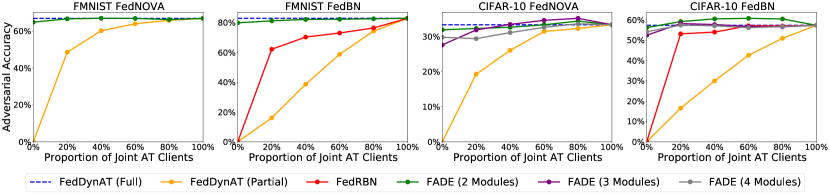
Figure 5: Adversarial accuracy when training with different proportions of resource-sufficient clients who perform joint AT.

We first compare FADE with other baselines in a setting where fixed $20\%$ clients can afford AT on the entire model, while the other $80\%$ clients can only afford ST on the entire model or AT on a single small module. Table 2 and Table 3 show the natural and adversarial accuracy of different training schemes on FMNIST and CIFAR-10 respectively. For FADE, we mix clients using different numbers of modules with different ratios in each scheme. For example, “FADE (2:2:3:3)” means that the clients with 1 module, 2 modules, 3 modules and 4 modules are mixed in a ratio of 2:2:3:3.

While neither partial FedDynAT nor FedRBN can maintain robustness under this resource constraint, the results show that FADE can attain almost the same or even higher accuracy and robustness compared to full FedDynAT (the constraint-free case). Additionally, the consistency in the performance of FADE with different mixes of clients shows the high compatibility of our flexible FDL framework.

We also conducted experiments with different proportions of resource-sufficient clients, as shown in Figure 5. In each setting, the resource-sufficient clients who perform joint AT are mixed with resource-constrained clients who perform joint ST or adopt FADE with a multi-module model partition (e.g., a 2-module partition in “FADE (2 Modules)”).

We can see that even in the worst case that none of the clients have enough resources to complete AT on the entire model, FADE can achieve robustness comparable to full FedDynAT. And with only $40\%$ resource-sufficient clients, FADE can attain almost the same robustness as full FedDynAT in most experiments, while the other baselines still have significant robustness gaps from full FedDynAT under this setting.

It is noteworthy that the results of FADE with $0\%$ resource-sufficient clients in Figure 5 can be viewed as a special baseline: naively deploying DGL in FL without differentiated model partitions. We can see that the performance of this baseline is always worse than FADE with differentiated model partitions when the proportion of resource-sufficient clients is larger than $0\%$.

4.4 The Influence of Auxiliary Weight Decay

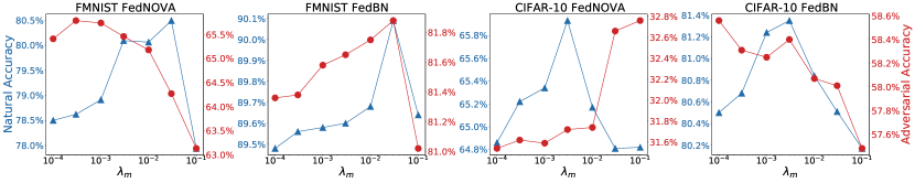
Figure 6: Natural accuracy (blue lines with triangle markers) and adversarial accuracy (red lines with circle markers) of FADE (2:8) with different auxiliary weight decay hyperparameter $\lambda_{m}$.

As we discussed in Section 3.3, the hyperparameter $\lambda_{m}$ for weight decay on the auxiliary model acts as an important role that balances natural accuracy and adversarial robustness. To show the influence of this hyperparameter, we conduct experiments on “FADE (2:8)” (or “FADE (2:8:0:0)”) with different $\lambda_{m}$ between $0.0001$ and $0.1$, and we plot the natural and adversarial accuracy in Figure 6.

We can observe that in all our settings, the natural accuracy increases first as we increase $\lambda_{m}$, and then goes down quickly. The growing part can be explained by our theory in Section 3.3 that the large auxiliary weight decay can alleviate the objective inconsistency and improve the performance. However, when we adopt an excessively large weight decay, the weight decay will drive the model away from optimum and lead to a performance drop, which is also commonly observed in the joint training process.

For the adversarial accuracy, the effects of $\lambda_{m}$ become more complicated, since larger $\lambda_{m}$ can decrease both $g_{m}$ and $\mu_{m}$, which affect the robustness in opposite ways. An increasing adversarial accuracy suggests that the effect of $g_{m}$ dominates, while a decreasing one suggests that the effect of $\mu_{m}$ dominates. Similarly to the natural accuracy, we observe that the adversarial accuracy grows first and then goes down in most cases, which implies a stronger effect of $g_{m}$ when $\lambda_{m}$ is small. And considering the increasing natural accuracy, adopting a moderately large $\lambda_{m}$ usually attains a better overall performance on clean and adversarial examples.

5 Related Works

Federated Learning. Client-wise heterogeneity is one of the challenges that hinder the practice of Federated Learning (FL). Many studies have tried to overcome the statistical heterogeneity in data (Karimireddy et al., 2019; Liang et al., 2019; Wang et al., 2020a; Tang et al., 2022) and the systematic heterogeneity in hardware (Li et al., 2018; Wang et al., 2020b; Li et al., 2021a). Beyond the heterogeneity, FL is also vulnerable to several kinds of attack, such as model poisoning attacks (Bhagoji et al., 2019; Sun et al., 2021) and adversarial examples (Zizzo et al., 2020; Shah et al., 2021). In this paper, we mainly focus on the adversarial examples and deal with the challenge in federated adversarial training under client-wise heterogeneity (Hong et al., 2021).

Adversarial Training. AT is well known for its high demand for computing resources, including computing power and memory capacity (Wong et al., 2020; Liu et al., 2020). Several fast AT algorithms have been proposed to reduce the computation in AT (Shafahi et al., 2019; Zhang et al., 2019), such as replacing PGD with FGSM (Andriushchenko & Flammarion, 2020; Wong et al., 2020) or using other regularization methods for robustness (Moosavi-Dezfooli et al., 2019; Qin et al., 2019). As a complement to these fast AT algorithms, FADE is proposed to reduce the memory requirement in AT, and we leave the combination of FADE and fast AT algorithms to future works.

Decoupled Greedy Learning. As deeper and deeper neural networks are used for better performance, the low efficiency of end-to-end (joint) training is exposed because it hinders the model parallelization and requires large memory for model parameters and intermediate results (Hettinger et al., 2017; Belilovsky et al., 2020). As an alternative, Decoupled Greedy Learning (DGL) is proposed, which decouples the whole neural network into several modules and trains them separately without gradient dependency (Marquez et al., 2018; Belilovsky et al., 2019, 2020; Wang et al., 2021). In contrast to allowing only one unified model partition in DGL, FADE fits better in FL with differentiated model partitions for heterogeneous clients. Additionally, FADE complements DGL with provable adversarial robustness and objective inconsistency alleviation, which allows FADE to maintain high adversarial and natural accuracy.

6 Conclusions

In this paper, we propose Federated Adversarial Decoupled Learning (FADE), a novel framework that enables federated adversarial training on heterogeneous resource-constrained edge devices. We theoretically analyze the convergence, robustness and objective inconsistency of FADE. Our experimental results reveal that FADE can significantly reduce both memory and computational requirements on small edge devices while maintaining almost the same accuracy and robustness as joint federated adversarial training.

Appendix A Convergence Analysis of Federated Decoupled Learning

A.1 Preliminary

In this section, we analyze the convergence property of Federated Decoupled Learning (FDL). Since FDL partitions the entire model with layers as the smallest unit, we only need to prove the convergence of each layer. We use $\bm{\omega}_{n}$ to denote all the parameters in layer $n$, and $m_{k}(n)$ to denote the module that contains layer $n$ on client $k$. We define the parameters other than $\bm{\omega}_{n}$ in module $m_{k}(n)$ as $\bm{\Omega}_{n,k}$. For notation simplicity, we also define ${\bm{z}}_{n-1,k}={\bm{z}}_{m_{k}(n)-1}$, and the locally supervised loss of layer $n$ on client $k$ as:

$$l_{n,k}^{(t,j)}({\bm{z}}_{n-1}^{(t)},y;\bm{\omega}_{n}^{(t,j)})=l_{m_{k}(n)}({\bm{z}}_{m_{k}(n)-1}^{(t)},y;\bm{\omega}_{n}^{(t,j)},\bm{\Omega}_{n,k}^{(t,j)}),$$ (17)

where $l_{n,k}^{(t,j)}$ changes every iteration because of the update of $\bm{\Omega}_{n,k}^{(t,j)}$. For simplicity, from now on we abridge $({\bm{z}},y)$ as ${\bm{z}}$. We let ${\bm{z}}_{n-1,k}^{(t,j)}$ follow the distribution with probability density $p_{n-1,k}^{(t)}({\mathbf{z}})$ at communication round $t$, and we define its converged density as $p_{n-1,k}^{*}({\mathbf{z}})$ with converged previous layers (Belilovsky et al., 2020). For some $\bm{\Omega}_{n,k}^{*}$, we define

$$L_{n,k}^{(t)}(\bm{\omega}_{n}^{(t)})=\mathbb{E}_{{\bm{z}}_{n-1,k}^{(t,j)}\sim p_{n-1,k}^{(t)}}\left[\frac{1}{\tau}\sum_{j=0}^{\tau-1}l_{n,k}^{(t,j)}({\bm{z}}_{n-1,k}^{(t,j)};\bm{\omega}_{n}^{(t)})\right];$$ (18)

$$L_{n}^{(t)}(\bm{\omega}_{n}^{(t)})=\sum_{k=1}^{N}q_{k}L_{n,k}^{(t)}(\bm{\omega}_{n}^{(t)});$$ (19)

$$L_{n,k}(\bm{\omega}_{n}^{(t)})=\mathbb{E}_{{\bm{z}}_{n-1,k}\sim p_{n-1,k}^{*}}\left[l_{n,k}^{*}({\bm{z}}_{n-1,k};\bm{\omega}_{n}^{(t)})\right]$$

$$=\mathbb{E}_{{\bm{z}}_{m_{k}(n)-1,k}\sim p_{m_{k}(n)-1,k}^{*}}\left[l_{m_{k}(n)}({\bm{z}}_{m_{k}(n)-1,k};\bm{\omega}_{n}^{(t)},\bm{\Omega}_{n,k}^{*})\right];$$ (20)

$$L_{n}(\bm{\omega}_{n}^{(t)})=\sum_{k=1}^{N}q_{k}L_{n,k}(\bm{\omega}_{n}^{(t)});$$ (21)

Following Belilovsky et al. (2020), we use the distance between the current density and the converged density below for our analysis:

$$\rho_{n}^{(t)}\triangleq\sum_{k=1}^{N}q_{k}\int\left|p_{n-1,k}^{(t)}({\mathbf{z}})-p_{n-1,k}^{*}({\mathbf{z}})\right|d{\mathbf{z}},$$ (22)

And we also define the following gap between $l_{n,k}^{(t)}$ and $l_{n,k}^{*}$:

$$\xi_{n}^{(t)}\triangleq\sum_{k=1}^{N}\sum_{j=0}^{\tau-1}\frac{q_{k}}{\tau}\left\|\mathbb{E}_{{\bm{z}}_{n-1,k}\sim p_{n-1}^{*}}\left[\nabla l_{n,k}^{(t,j)}({\bm{z}}_{n-1,k};\omega_{n}^{(t)})-\nabla l_{n,k}^{*}({\bm{z}}_{n-1,k};\omega_{n}^{(t)})\right]\right\|^{2}.$$ (23)

We will discuss the convergence of $L_{n}(\bm{\omega}_{n})$ for each layer $n$. Without specifying, all the gradients ($\nabla L$ or $\nabla l$) in the following analysis are with respect to $\bm{\omega}_{n}$. Following Belilovsky et al. (2020) and Wang et al. (2020b), we make the common assumptions below.

Assumption A.1 ($\mathcal{L}$-smoothness (Belilovsky et al., 2020; Wang et al., 2020b)).

$L_{n}$ is differentiable with respect to $\bm{\omega}_{n}^{(t)}$ and its gradient is $\mathcal{L}_{n}$-Lipschitz for all $t$. Similarly, $l_{n,k}^{(t,j)}$ is differentiable with respect to $\bm{\omega}_{n,k}$ and its gradient is $\widetilde{\mathcal{L}}_{n}$-Lipschitz for all $t,j$ and $k$.

Assumption A.2 (Robbins-Monro conditions (Belilovsky et al., 2020)).

The learning rates satisfy $\sum_{t=0}^{\infty}\eta_{t}=\infty$ yet $\sum_{t=0}^{\infty}\eta_{t}^{2}<\infty$.

Assumption A.3 (Finite variance (Belilovsky et al., 2020)).

There exists some positive constant $G$ such that $\forall t,j$ and $\forall k$, $\mathbb{E}_{{\bm{z}}_{n-1,k}^{(t,j)}\sim p_{n-1,k}^{(t,j)}}\left[\left\|\nabla l_{n,k}^{(t,j)}({\bm{z}}_{n-1,k}^{(t,j)};\bm{\omega}_{n})\right\|^{2}\right]\leq G$ and $\mathbb{E}_{{\bm{z}}_{n-1,k}\sim p_{n-1}^{*}}\left[\left\|\nabla l_{n,k}^{*}({\bm{z}}_{n-1,k};\bm{\omega}_{n})\right\|^{2}\right]\leq G$ at any $\bm{\omega}_{n}$.

Assumption A.4 (Convergence of the previous modules and $\bm{\Omega}_{n,k}$ (Belilovsky et al., 2020)).

We assume that $\sum_{t=0}^{\infty}\rho_{n}^{(t)}<\infty$ and $\sum_{t=0}^{\infty}{\xi_{n}^{(t)}}<\infty$.

A.2 Proof of Theorem 3.1

With all above assumptions, we get the following theorem that guarantees the convergence of Federated Decoupled Learning.

Theorem A.5.

Under A.1 - A.4, given a client sampling method that satisfies $\Pr(k\in{\mathbb{S}}_{n}^{(t)})=p$ for any client $k$, Federated Decoupled Learning converges as follows:

$$\inf_{t\leq T}\mathbb{E}\left[\left\|\nabla L_{n}\left(\bm{\omega}_{n}^{(t)}\right)\right\|^{2}\right]$$

$$\leq \mathcal{O}\left(\frac{1}{\sum_{t=0}^{T}\eta_{t}}\right)+\mathcal{O}\left(\frac{\sum_{t=0}^{T}{\rho_{n}^{(t)}}\eta_{t}}{\sum_{t=0}^{T}\eta_{t}}\right)+\mathcal{O}\left(\frac{\sum_{t=0}^{T}{\xi_{n}^{(t)}}\eta_{t}}{\sum_{t=0}^{T}\eta_{t}}\right)+\mathcal{O}\left(\frac{\sum_{t=0}^{T}\eta_{t}^{2}}{\sum_{t=0}^{T}\eta_{t}}\right).$$ (24)

Proof.

We consider the following SGD scheme with learning rate $\left\{\eta_{t}\right\}_{t}$:

$$\bm{\omega}_{n}^{(t+1)}=\bm{\omega}_{n}^{(t)}-\eta_{t}\tau\frac{\sum_{k\in{\mathbb{S}}_{n}^{(t)}}q_{k}\bm{h}_{n,k}^{(t)}}{p},$$ (25)

where ${\mathbb{S}}_{n}^{(t)}=\{k\in{\mathbb{S}}^{(t)}:n\in m_{k}^{t}\}$ which is defined in Equation 11. And ${\bm{h}_{n,k}^{(t)}}$ is defined as

$$\bm{h}_{n,k}^{(t)}=\frac{1}{\tau}\sum_{j=0}^{\tau-1}\nabla l_{n,k}^{(t,j)}({\bm{z}}_{n-1,k}^{(t,j)};\bm{\omega}_{n,k}^{(t,j)}).$$

According to the Lipschitz-smooth assumption for the global objective function $L_{n}$, it follows that

$$\mathbb{E}\left[L_{n}\left(\bm{\omega}_{n}^{(t+1)}\right)\right]-L_{n}\left(\bm{\omega}_{n}^{(t)}\right)$$

$$\leq -\eta_{t}\tau\underbrace{\mathbb{E}\left[\left\langle\nabla L_{n}\left(\bm{\omega}_{n}^{(t)}\right),\frac{\sum_{k\in{\mathbb{S}}_{n}^{(t)}}q_{k}\bm{h}_{n,k}^{(t)}}{p}\right\rangle\right]}_{T_{1}}+\frac{\eta_{t}^{2}\tau^{2}\mathcal{L}_{n}}{2p^{2}}\underbrace{\mathbb{E}\left[\left\|\sum_{k\in{\mathbb{S}}_{n}^{(t)}}q_{k}\bm{h}_{n,k}^{(t)}\right\|^{2}\right]}_{T_{2}},$$ (26)

where expectation is taken over the minibatch as well as ${\mathbb{S}}_{n}^{(t)}$.

Similar to the proof in (Wang et al., 2020b), to bound the $T_{1}$ in Inequality (26), we should notice that

$$T_{1}= \mathbb{E}\left[\left\langle\nabla L_{n}\left(\bm{\omega}_{n}^{(t)}\right),\frac{\sum_{k\in{\mathbb{S}}_{n}^{(t)}}q_{k}\bm{h}_{n,k}^{(t)}}{p}\right\rangle\right]$$

$$= \left\langle\nabla L_{n}\left(\bm{\omega}_{n}^{(t)}\right),\frac{\mathbb{E}\left[\sum_{k\in{\mathbb{S}}_{n}^{(t)}}q_{k}\bm{h}_{n,k}^{(t)}\right]}{p}\right\rangle$$

$$= \left\langle\nabla L_{n}\left(\bm{\omega}_{n}^{(t)}\right),\frac{\sum_{k=1}^{N}\mathbb{E}\left[q_{k}\bm{h}_{n,k}^{(t)}1_{[k\in{\mathbb{S}}_{n}^{(t)}]}\right]}{p}\right\rangle$$

$$= \left\langle\nabla L_{n}\left(\bm{\omega}_{n}^{(t)}\right),{\sum_{k=1}^{N}q_{k}\mathbb{E}\bm{h}_{n,k}^{(t)}}\right\rangle$$

$$= \frac{1}{2}\left\|\nabla L_{n}\left(\bm{\omega}_{n}^{(t)}\right)\right\|^{2}+\frac{1}{2}\left\|{\sum_{k=1}^{N}q_{k}\mathbb{E}\bm{h}_{n,k}^{(t)}}\right\|^{2}-\frac{1}{2}\left\|\nabla L_{n}\left(\bm{\omega}_{n}^{(t)}\right)-{\sum_{k=1}^{N}q_{k}\mathbb{E}\bm{h}_{n,k}^{(t)}}\right\|^{2}$$ (27)

$$\geq \frac{1}{2}\left\|\nabla L_{n}\left(\bm{\omega}_{n}^{(t)}\right)\right\|^{2}-\frac{1}{2}\left\|\nabla L_{n}\left(\bm{\omega}_{n}^{(t)}\right)-{\sum_{k=1}^{N}q_{k}\mathbb{E}\bm{h}_{n,k}^{(t)}}\right\|^{2}$$

$$\geq \frac{1}{2}\left\|\nabla L_{n}\left(\bm{\omega}_{n}^{(t)}\right)\right\|^{2}-\left\|\nabla L_{n}^{(t)}\left(\bm{\omega}_{n}^{(t)}\right)-{\sum_{k=1}^{N}q_{k}\mathbb{E}\bm{h}_{n,k}^{(t)}}\right\|^{2}-\left\|\nabla L_{n}\left(\bm{\omega}_{n}^{(t)}\right)-\nabla L_{n}^{(t)}(\bm{\omega}_{n}^{(t)})\right\|^{2}$$ (28)

$$\geq \frac{1}{2}\left\|\nabla L_{n}\left(\bm{\omega}_{n}^{(t)}\right)\right\|^{2}-{\sum_{k=1}^{N}q_{k}\left\|\mathbb{E}\bm{h}_{n,k}^{(t)}-\nabla L_{n,k}^{(t)}(\bm{\omega}_{n}^{(t)})\right\|^{2}}-\left\|\nabla L_{n}\left(\bm{\omega}_{n}^{(t)}\right)-\nabla L_{n}^{(t)}(\bm{\omega}_{n}^{(t)})\right\|^{2}.$$ (29)

Equation 27 uses the fact: $2\langle a,b\rangle=\|a\|^{2}+\|b\|^{2}-\|a-b\|^{2}$, and Inequality (28) uses the fact: $\|a+b\|^{2}\leq 2\|a\|^{2}+2\|b\|^{2}$. Inequality (29) uses $L_{n}^{(t)}={\sum_{k=1}^{N}q_{k}L_{n,k}^{(t)}}$ and Jenson’s inequality $\left\|\sum_{i=k}^{N}q_{k}{\bm{a}}_{i}\right\|^{2}\leq\sum_{k=1}^{N}q_{k}\left\|{\bm{a}}_{i}\right\|^{2}$.

For the second term in $T_{1}$, we have

$$\left\|\mathbb{E}\bm{h}_{n,k}^{(t)}-\nabla L_{n,k}^{(t)}(\bm{\omega}_{n}^{(t)})\right\|^{2} =\left\|\frac{1}{\tau}\sum_{j=0}^{\tau-1}\mathbb{E}\left[\nabla l_{n,k}^{(t,j)}({\bm{z}}_{n-1,k}^{(t,j)};\bm{\omega}_{n,k}^{(t,j)})-\nabla l_{n,k}^{(t,j)}({\bm{z}}_{n-1,k}^{(t,j)};\bm{\omega}_{n}^{(t,0)})\right]\right\|^{2}$$

$$\leq\frac{1}{\tau}\sum_{j=0}^{\tau-1}\mathbb{E}\left\|\nabla l_{n,k}^{(t,j)}({\bm{z}}_{n-1,k}^{(t,j)};\bm{\omega}_{n,k}^{(t,j)})-\nabla l_{n,k}^{(t,j)}({\bm{z}}_{n-1,k}^{(t,j)};\bm{\omega}_{n}^{(t,0)})\right\|^{2}$$

$$\leq\frac{\mathcal{\widetilde{L}}_{n}^{2}}{\tau}\sum_{j=0}^{\tau-1}\mathbb{E}\left\|\bm{\omega}_{n,k}^{(t,j)}-\bm{\omega}_{n,k}^{(t,0)}\right\|^{2}.$$

And we know that

$$\mathbb{E}\left\|\bm{\omega}_{n,k}^{(t,j)}-\bm{\omega}_{n,k}^{(t,0)}\right\|^{2} =\eta_{t}^{2}\mathbb{E}\left\|\sum_{s=0}^{j-1}\nabla l_{n,k}^{(t,s)}\right\|^{2}$$

$$\leq\eta_{t}^{2}j\sum_{s=0}^{j-1}\mathbb{E}\left\|\nabla l_{n,k}^{(t,s)}\right\|^{2}$$

$$\leq\eta_{t}^{2}j^{2}G.$$

Thus we get

$$\left\|\mathbb{E}\bm{h}_{n,k}^{(t)}-\nabla L_{n,k}^{(t)}(\bm{\omega}_{n}^{(t)})\right\|^{2} \leq\frac{\mathcal{\widetilde{L}}_{n}^{2}}{\tau}\sum_{j=0}^{\tau-1}\mathbb{E}\left\|\bm{\omega}_{n,k}^{(t,j)}-\bm{\omega}_{n,k}^{(t,0)}\right\|^{2}$$

$$\leq\frac{\mathcal{\widetilde{L}}_{n}^{2}}{\tau}\sum_{j=0}^{\tau-1}\eta_{t}^{2}j^{2}G$$

$$\leq\frac{\tau^{2}}{2}\mathcal{\widetilde{L}}_{n}^{2}\eta_{t}^{2}G.$$ (30)

For the third term in $T_{1}$, based on the proof of Lemma 3.2 in Belilovsky et al. (2020), we have

$$\left\|\nabla L_{n}\left(\bm{\omega}_{n}^{(t)}\right)-\nabla L_{n}^{(t)}\left(\bm{\omega}_{n}^{(t)}\right)\right\|^{2}$$

$$= \left\|\sum_{k}q_{k}\mathbb{E}_{{\bm{z}}\sim p_{n-1,k}^{*}}\left[\nabla l_{n,k}^{*}({\bm{z}};\bm{\omega}_{n}^{(t)})\right]-\sum_{k}q_{k}\mathbb{E}_{{\bm{z}}^{(t,j)}\sim p_{n-1,k}^{(t)}}\left[\frac{1}{\tau}\sum_{j}\nabla l_{n,k}^{(t,j)}({\bm{z}}^{(t,j)};\bm{\omega}_{n}^{(t)})\right]\right\|^{2}$$

$$= \left\|\frac{1}{\tau}\sum_{k}q_{k}\sum_{j}\left(\mathbb{E}_{{\bm{z}}\sim p_{n-1,k}^{*}}\left[\nabla l_{n,k}^{*}({\bm{z}};\bm{\omega}_{n}^{(t)})\right]-\mathbb{E}_{{\bm{z}}\sim p_{n-1,k}^{(t)}}\left[\nabla l_{n,k}^{(t,j)}({\bm{z}};\bm{\omega}_{n}^{(t)})\right]\right)\right\|^{2}$$

$$\leq \frac{1}{\tau}\sum_{k}q_{k}\sum_{j}\left\|\mathbb{E}_{{\bm{z}}\sim p_{n-1,k}^{*}}\left[\nabla l_{n,k}^{*}({\bm{z}};\bm{\omega}_{n}^{(t)})\right]-\mathbb{E}_{{\bm{z}}\sim p_{n-1,k}^{(t)}}\left[\nabla l_{n,k}^{(t,j)}({\bm{z}};\bm{\omega}_{n}^{(t)})\right]\right\|^{2}$$

$$\leq \frac{2}{\tau}\sum_{k}q_{k}\sum_{j}\left\|\int\nabla l_{n,k}^{(t,j)}({\bm{z}};\bm{\omega}_{n}^{(t)})p_{n-1,k}^{(t)}({\mathbf{z}})d{\mathbf{z}}-\int\nabla l_{n,k}^{(t,j)}({\bm{z}};\bm{\omega}_{n}^{(t)})p_{n-1,k}^{*}({\mathbf{z}})d{\mathbf{z}}\right\|^{2}$$

$$+\frac{2}{\tau}\sum_{k}q_{k}\sum_{j}\left\|\mathbb{E}_{{\bm{z}}\sim p_{n-1,k}^{*}}\left[\nabla l_{n,k}^{(t,j)}({\bm{z}};\bm{\omega}_{n}^{(t)})-\nabla l_{n,k}^{*}({\bm{z}};\bm{\omega}_{n}^{(t)})\right]\ \right\|^{2}$$

$$\leq \frac{2}{\tau}\sum_{k}q_{k}\sum_{j}\left(\int\left\|\nabla l_{n,k}^{(t,j)}({\mathbf{z}};\bm{\omega}_{n}^{(t)})\right\|\sqrt{|p_{n-1,k}^{(t)}({\mathbf{z}})-p_{n-1,k}^{*}({\mathbf{z}})||p_{n-1,k}^{(t)}({\mathbf{z}})-p_{n-1,k}^{*}({\mathbf{z}})|}d{\mathbf{z}}\right)^{2}$$

$$+2\xi_{n}^{(t)}$$

$$\leq \frac{2}{\tau}\sum_{k}q_{k}\sum_{j}\int\left\|\nabla l_{n,k}^{(t,j)}({\mathbf{z}};\bm{\omega}_{n}^{(t)})\right\|^{2}{|p_{n-1,k}^{(t)}({\mathbf{z}})-p_{n-1}^{*}({\mathbf{z}})|}d{\mathbf{z}}\int|p_{n-1,k}^{(t)}({\mathbf{z}})-p_{n-1,k}^{*}({\mathbf{z}})|d{\mathbf{z}}$$

$$+2\xi_{n}^{(t)}$$

$$\leq \frac{2}{\tau}\sum_{k}q_{k}\int|p_{n-1,k}^{(t)}({\mathbf{z}})-p_{n-1,k}^{*}({\mathbf{z}})|d{\mathbf{z}}\sum_{j}\int\left\|\nabla l_{n,k}^{(t,j)}({\mathbf{z}};\bm{\omega}_{n}^{(t)})\right\|^{2}{\left(p_{n-1,k}^{(t)}({\mathbf{z}})+p_{n-1,k}^{*}({\mathbf{z}})\right)}d{\mathbf{z}}$$

$$+2\xi_{n}^{(t)}$$

$$\leq 4G\rho_{n}^{(t)}+2\xi_{n}^{(t)}.$$ (31)

Plugging Equation 30 and Equation 31 back to Equation 29, we have

$$T_{1} \geq\frac{1}{2}\left\|\nabla L_{n}\left(\bm{\omega}_{n}^{(t)}\right)\right\|^{2}-\frac{\tau^{2}}{2}\mathcal{\widetilde{L}}_{n}^{2}\eta_{t}^{2}G-4G\rho_{n}^{(t)}-2\xi_{n}^{(t)}.$$ (32)

Now we turn to bound $T_{2}$. With the fact that $\sum_{k\in{\mathbb{S}}_{n}^{(t)}}q_{k}\leq 1$, we have:

$$T_{2} =\mathbb{E}\left[\left(\sum_{k\in{\mathbb{S}}_{n}^{(t)}}q_{k}\right)^{2}\left\|\frac{\sum_{k\in{\mathbb{S}}_{n}^{(t)}}q_{k}\bm{h}_{n,k}^{(t)}}{\sum_{k\in{\mathbb{S}}_{n}^{(t)}}q_{k}}\right\|^{2}\right]$$

$$\leq\mathbb{E}\left[\sum_{k\in{\mathbb{S}}_{n}^{(t)}}q_{k}\left\|\bm{h}_{n,k}^{(t)}\right\|^{2}\right]$$

$$\leq\mathbb{E}\left[\frac{\sum_{k\in{\mathbb{S}}_{n}^{(t)}}q_{k}\sum_{j=0}^{\tau-1}\left\|\nabla l_{n,k}^{(t,j)}({\bm{z}}_{n-1,k}^{(t,j)};\bm{\omega}_{n,k}^{(t,j)})\right\|^{2}}{\tau}\right]$$

$$=\frac{\sum_{k=1}^{N}q_{k}\sum_{j=0}^{\tau-1}\mathbb{E}\left\|\nabla l_{n,k}^{(t,j)}({\bm{z}}_{n-1,k}^{(t,j)};\bm{\omega}_{n,k}^{(t,j)})\right\|^{2}\mathbb{E}_{{\mathbb{S}}_{n}^{(t)}}\left[1_{k\in{\mathbb{S}}_{n}^{(t)}}\right]}{\tau}$$

$$\leq pG.$$ (33)

Instituting $T_{1}$ and $T_{2}$ in Equation 26 with Equation 32 and Equation 33 respectively, we have

$$\mathbb{E}\left[L_{n}\left(\bm{\omega}_{n}^{(t+1)}\right)\right]-L_{n}\left(\bm{\omega}_{n}^{(t)}\right)$$

$$\leq -\eta_{t}\tau\left[\frac{1}{2}\left\|\nabla L_{n}\left(\bm{\omega}_{n}^{(t)}\right)\right\|^{2}-\frac{\tau^{2}}{2}\mathcal{\widetilde{L}}_{n}^{2}\eta_{t}^{2}G-4G\rho_{n}^{(t)}-2\xi_{n}^{(t)}\right]+\frac{\eta_{t}^{2}\tau^{2}\mathcal{L}_{n}G}{2p}.$$ (34)

Assuming that $\eta_{t}\leq 1$ and $L_{n}>0$, rearranging Equation 34, taking the expectation and averaging across all rounds, one can obtain

$$\frac{1}{2}\sum_{t=0}^{T}\eta_{t}\mathbb{E}\left[\left\|\nabla L_{n}\left(\bm{\omega}_{n}^{(t)}\right)\right\|^{2}\right]$$

$$\leq \frac{1}{\tau}\left(L_{n}\left(\bm{\omega}_{n}^{(0)}\right)-\mathbb{E}\left[L_{n}\left(\bm{\omega}_{n}^{(T+1)}\right)\right]\right)+A\sum_{t=0}^{T}\eta_{t}^{2}+B\sum_{t=0}^{T}\eta_{t}\rho_{n}^{(t)}+C\sum_{t=0}^{T}\eta_{t}\xi_{n}^{(t)}$$

$$\leq \frac{1}{\tau}L_{n}\left(\bm{\omega}_{n}^{(0)}\right)+A\sum_{t=0}^{T}\eta_{t}^{2}+B\sum_{t=0}^{T}\eta_{t}\rho_{n}^{(t)}+C\sum_{t=0}^{T}\eta_{t}\xi_{n}^{(t)},$$

where $A,B$ and $C$ are some positive constants. Now we get our final result:

$$\inf_{t\leq T}\mathbb{E}\left[\left\|\nabla L_{n}\left(\bm{\omega}_{n}^{(t)}\right)\right\|^{2}\right]\leq\frac{1}{\sum_{t=0}^{T}\eta_{t}}\sum_{t=0}^{T}\eta_{t}\mathbb{E}\left[\left\|\nabla L_{n}\left(\bm{\omega}_{n}^{(t)}\right)\right\|^{2}\right]$$

$$\leq \mathcal{O}\left(\frac{1}{\sum_{t=0}^{T}\eta_{t}}\right)+\mathcal{O}\left(\frac{\sum_{t=0}^{T}{\rho_{n}^{(t)}}\eta_{t}}{\sum_{t=0}^{T}\eta_{t}}\right)+\mathcal{O}\left(\frac{\sum_{t=0}^{T}{\xi_{n}^{(t)}}\eta_{t}}{\sum_{t=0}^{T}\eta_{t}}\right)+\mathcal{O}\left(\frac{\sum_{t=0}^{T}\eta_{t}^{2}}{\sum_{t=0}^{T}\eta_{t}}\right).$$

It is simple to verify that $\frac{1}{\sum_{t=0}^{T}\eta_{t}}\to 0$ and $\frac{\sum_{t=0}^{T}\eta_{t}^{2}}{\sum_{t=0}^{T}\eta_{t}}\to 0$ if $T\to\infty$. As for $\frac{\sum_{t=0}^{T}{\rho_{n}^{(t)}}\eta_{t}}{\sum_{t=0}^{T}\eta_{t}}$, according to the Cauchy-Schwartz inequality, we have

$${\sum_{t=0}^{T}{\rho_{n}^{(t)}}\eta_{t}} =\sum_{t=0}^{T}\sqrt{\rho_{n}^{(t)}}\left(\sqrt{\rho_{n}^{(t)}}\eta_{t}\right)$$

$$\leq\sqrt{\left(\sum_{t=0}^{T}{\rho_{n}^{(t)}}\right)\left(\sum_{t=0}^{T}{\rho_{n}^{(t)}}\eta_{t}^{2}\right)}$$

$$\leq\sqrt{\left(\sum_{t=0}^{T}{\rho_{n}^{(t)}}\right)\left(\sum_{t=0}^{T}{\rho_{n}^{(t)}}\right)\left(\sum_{t=0}^{T}\eta_{t}^{2}\right)}$$

$$<\infty.$$

Hence, we also have $\frac{\sum_{t=0}^{T}{\rho_{n}^{(t)}}\eta_{t}}{\sum_{t=0}^{T}\eta_{t}}\to 0$ if $T\to\infty$. Similarly, we get the same result for $\frac{\sum_{t=0}^{T}{\xi_{n}^{(t)}}\eta_{t}}{\sum_{t=0}^{T}\eta_{t}}$. In conclusion, we get the result in Section 3.1:

$$\lim_{T\rightarrow\infty}\inf_{t\leq T}\mathbb{E}\left\|\nabla L_{n}\left(\bm{\omega}_{n}^{(t)}\right)\right\|^{2}=0.$$

We notice that there is a minor difference between the update rule in Equation 11 and in Equation 25, where we can bridge the gap by setting the original learning rate in Equation 11 as $\eta_{t}=\eta_{t}\sum_{i\in{\mathbb{S}}_{n}^{(t)}}q_{k}/p$.

∎

Appendix B Proofs of Theorem 3.2, Lemma 3.4 and Additional Analysis

B.1 Proof of Theorem 3.2

Theorem B.1.

Assume that $\tilde{l}_{m}({\bm{z}}_{m},y)$ is $\mu_{m}$-strongly convex in ${\bm{z}}_{m}$ for each module $m$. We can guarantee that the entire model has a joint $(\epsilon_{0},c_{M})$-robustness in $l({\bm{x}},y)$, if each module $m\leq M$ has local $(\epsilon_{m-1},c_{m})$-robustness in $l_{m}({\bm{z}}_{m-1},y)$, and

$$\quad\epsilon_{m}\geq\frac{g_{m}}{\mu_{m}}+\sqrt{\frac{2c_{m}}{\mu_{m}}+\frac{g_{m}^{2}}{\mu_{m}^{2}}},$$ (35)

where $g_{m}=\left\|\nabla_{{\bm{z}}_{m}}\tilde{l}_{m}({\bm{z}}_{m},y)\right\|$.

Proof.

We only need to prove the joint robustness of the concatenation of module $m$ and $(m+1)$ given the local robustness of them separately, and then we can use deduction to get the joint robustness of the entire model given the local robustness of all modules.

For a module $m$ and any perturbation $\bm{\delta}_{m-1}\in\{\bm{\delta}_{m-1}:\|\bm{\delta}_{m-1}\|\leq\epsilon_{m-1}\}$ at its input, let ${\bm{r}}=f_{m}({\bm{z}}_{m-1}+\bm{\delta}_{m-1})-f_{m}({\bm{z}}_{m-1})$. Given $\mu_{m}$-strongly convexity and $(\epsilon_{m-1},c_{m})$-robustness in $\tilde{l}_{m}({\bm{z}}_{m},y)$, we have

$$\nabla_{{\bm{z}}_{m}}\tilde{l}_{m}({\bm{z}}_{m},y)^{T}{\bm{r}}+\frac{\mu_{m}}{2}\|r\|^{2}\leq\tilde{l}_{m}({\bm{z}}_{m}+{\bm{r}},y)-\tilde{l}_{m}({\bm{z}}_{m},y)\leq c_{m}$$ (36)

$$\Rightarrow \frac{\mu_{m}}{2}\left[\left\|{\bm{r}}+\frac{\nabla_{{\bm{z}}_{m}}\tilde{l}_{m}({\bm{z}}_{m},y)}{\mu_{m}}\right\|^{2}-\frac{\|\nabla_{{\bm{z}}_{m}}\tilde{l}_{m}({\bm{z}}_{m},y)\|^{2}}{\mu_{m}^{2}}\right]\leq c_{m}$$ (37)

$$\Rightarrow \left\|{\bm{r}}+\frac{\nabla_{{\bm{z}}_{m}}\tilde{l}_{m}({\bm{z}}_{m},y)}{\mu_{m}}\right\|\leq\sqrt{\frac{2c_{m}}{\mu_{m}}+\frac{\|\nabla_{{\bm{z}}_{m}}\tilde{l}_{m}({\bm{z}}_{m},y)\|^{2}}{\mu_{m}^{2}}}$$ (38)

$$\Rightarrow \|{\bm{r}}\|\leq\frac{\|\nabla_{{\bm{z}}_{m}}\tilde{l}_{m}({\bm{z}}_{m},y)\|}{\mu_{m}}+\sqrt{\frac{2c_{m}}{\mu_{m}}+\frac{\|\nabla_{{\bm{z}}_{m}}\tilde{l}_{m}({\bm{z}}_{m},y)\|^{2}}{\mu_{m}^{2}}}=\frac{g_{m}}{\mu_{m}}+\sqrt{\frac{2c_{m}}{\mu_{m}}+\frac{g_{m}^{2}}{\mu_{m}^{2}}}.$$ (39)

And we know that

$$\epsilon_{m}\geq\frac{g_{m}}{\mu_{m}}+\sqrt{\frac{2c_{m}}{\mu_{m}}+\frac{g_{m}^{2}}{\mu_{m}^{2}}}\geq\|{\bm{r}}\|,$$ (40)

which gives us

$$\forall\bm{\delta}_{m-1}\in\{\bm{\delta}_{m-1}:\|\bm{\delta}_{m-1}\|\leq\epsilon_{m-1}\},\|f_{m}({\bm{z}}_{m-1}+\bm{\delta}_{m-1})-f_{m}({\bm{z}}_{m-1})\|\leq\epsilon_{m}.$$ (41)

With the $(\epsilon_{m},c_{m+1})$-robustness of module $(m+1)$, we have the joint robustness of the concatenation of $m$ and $(m+1)$:

$$\forall\bm{\delta}_{m-1}\in\{\bm{\delta}_{m-1}:\|\bm{\delta}_{m-1}\|\leq\epsilon_{m-1}\},$$

$$l_{m+1}(f_{m}({\bm{z}}_{m-1}+\bm{\delta}_{m-1}),y)-l_{m+1}(f_{m}({\bm{z}}_{m-1}),y)\leq c_{m+1}.$$ (42)

∎

B.2 Proof of Lemma 3.4

Lemma B.2.

Assume that $\tilde{l}_{m}({\bm{z}}_{m},y)$ and $\tilde{l}^{\prime}_{m}({\bm{z}}_{m},y)$ are $\beta_{m},\beta^{\prime}_{m}$-smooth in ${\bm{z}}_{m}$ for a module $m$. If there exist $\tilde{c}_{m}$, $\tilde{c}^{\prime}_{m}$, and $r\geq\sqrt{2\frac{\tilde{c}_{m}+\tilde{c}^{\prime}_{m}}{\beta_{m}+\beta^{\prime}_{m}}}$, such that the auxiliary model has $(r,\tilde{c}_{m})$-robustness in $\tilde{l}_{m}({\bm{z}}_{m},y)$, and the backbone network has $(r,\tilde{c}^{\prime}_{m})$-robustness in $\tilde{l}^{\prime}_{m}({\bm{z}}_{m},y)$, then we have:

$$\|\nabla_{{\bm{w}}_{m}}l-\nabla_{{\bm{w}}_{m}}l_{m}\|\leq\left\|\frac{\partial{\bm{z}}_{m}}{\partial{\bm{w}}_{m}}\right\|\sqrt{2(\tilde{c}_{m}+\tilde{c}^{\prime}_{m})(\beta_{m}+\beta^{\prime}_{m})}.$$ (43)

Proof.

With the chain rule, we know that

$$\nabla_{{\bm{w}}_{m}}l-\nabla_{{\bm{w}}_{m}}l_{m}=\frac{\partial{\bm{z}}_{m}}{\partial{\bm{w}}_{m}}\frac{\partial(l-l_{m})}{\partial{\bm{z}}_{m}}=\frac{\partial{\bm{z}}_{m}}{\partial{\bm{w}}_{m}}\frac{\partial(\tilde{l}^{\prime}_{m}-\tilde{l}_{m})}{\partial{\bm{z}}_{m}},$$ (44)

and thus

$$\|\nabla_{{\bm{w}}_{m}}l-\nabla_{{\bm{w}}_{m}}l_{m}\|\leq\left\|\frac{\partial{\bm{z}}_{m}}{\partial{\bm{w}}_{m}}\right\|\left\|\frac{\partial(\tilde{l}^{\prime}_{m}-\tilde{l}_{m})}{\partial{\bm{z}}_{m}}\right\|.$$ (45)

We now need to find the upper bound of the second factor. We define $h({\bm{z}}_{m})=\tilde{l}^{\prime}_{m}({\bm{z}}_{m},y)-\tilde{l}_{m}({\bm{z}}_{m},y)$, which is $(\beta_{m}+\beta_{m}^{\prime})$-smooth in ${\bm{z}}_{m}$. For any $\bm{\delta}_{m},\|\bm{\delta}_{m}\|\leq r$, with the $(r,\tilde{c}_{m})$-robustness in $\tilde{l}_{m}({\bm{z}}_{m},y)$ and $(r,\tilde{c}_{m}^{\prime})$-robustness in $\tilde{l}^{\prime}_{m}({\bm{z}}_{m},y)$, we have

$$|h({\bm{z}}_{m}+\bm{\delta}_{m})-h({\bm{z}}_{m})| \leq|\tilde{l}_{m}({\bm{z}}_{m}+\bm{\delta}_{m},y)-\tilde{l}_{m}({\bm{z}}_{m},y)|+|\tilde{l}^{\prime}_{m}({\bm{z}}_{m}+\bm{\delta}_{m},y)-\tilde{l}^{\prime}_{m}({\bm{z}}_{m},y)|$$

$$\leq\tilde{c}_{m}+\tilde{c}_{m}^{\prime}.$$ (46)

And with the $(\beta_{m}+\beta_{m}^{\prime})$-smoothness, we know that

$$\left(\frac{\partial h({\bm{z}}_{m})}{\partial{\bm{z}}_{m}}\right)^{T}\bm{\delta}_{m}-\frac{\beta_{m}+\beta_{m}^{\prime}}{2}\|\bm{\delta}_{m}\|^{2}\leq h({\bm{z}}_{m}+\bm{\delta}_{m})-h({\bm{z}}_{m})\leq\tilde{c}_{m}+\tilde{c}_{m}^{\prime}.$$ (47)

The maximum of the LHS is achieved when $\bm{\delta}^{*}_{m}=\frac{1}{\beta_{m}+\beta_{m}^{\prime}}\frac{\partial h({\bm{z}}_{m})}{\partial{\bm{z}}_{m}}$, and thus we get

$$\frac{1}{2(\beta_{m}+\beta_{m}^{\prime})}\left\|\frac{\partial h({\bm{z}}_{m})}{\partial{\bm{z}}_{m}}\right\|^{2}\leq\tilde{c}_{m}+\tilde{c}_{m}^{\prime}$$ (48)

$$\Rightarrow \left\|\frac{\partial h({\bm{z}}_{m})}{\partial{\bm{z}}_{m}}\right\|\leq\sqrt{2(\tilde{c}_{m}+\tilde{c}_{m}^{\prime})(\beta_{m}+\beta_{m}^{\prime})}.$$ (49)

To check the achievability of this maximum, we have

$$\|\bm{\delta}^{*}_{m}\|=\frac{1}{\beta_{m}+\beta_{m}^{\prime}}\left\|\frac{\partial h({\bm{z}}_{m})}{\partial{\bm{z}}_{m}}\right\|\leq\sqrt{2\frac{\tilde{c}_{m}+\tilde{c}^{\prime}_{m}}{\beta_{m}+\beta^{\prime}_{m}}}\leq r.$$ (50)

Thus, we get our final result

$$\|\nabla_{{\bm{w}}_{m}}l-\nabla_{{\bm{w}}_{m}}l_{m}\|\leq\left\|\frac{\partial{\bm{z}}_{m}}{\partial{\bm{w}}_{m}}\right\|\sqrt{2(\tilde{c}_{m}+\tilde{c}^{\prime}_{m})(\beta_{m}+\beta^{\prime}_{m})}.$$ (51)

∎

B.3 Case Study: Linear Auxiliary Output Model

For a linear auxiliary output model $\bm{\theta}_{m}=\{{\bm{W}}_{m},{\bm{b}}_{m}\}$, the cross-entropy loss is given as

$$\tilde{l}({\bm{z}}_{m},{\bm{y}})=\mathcal{L}(\sigma({\bm{W}}_{m}^{T}{\bm{z}}_{m}+{\bm{b}}_{m}),{\bm{y}}),$$ (52)

where $\mathcal{L}({\bm{p}},{\bm{y}})=-\sum_{i=1}y_{i}\log(p_{i})$ and $\sigma({\bm{q}})_{i}=\exp(q_{i})/(\sum_{j}\exp(q_{j}))$ are cross-entropy loss and softmax function respectively. Let ${\bm{p}}_{m}=\sigma({\bm{W}}_{m}^{T}{\bm{z}}_{m}+{\bm{b}}_{m})$, we know that

$$\nabla_{{\bm{z}}_{m}}\tilde{l}({\bm{z}}_{m},{\bm{y}})={\bm{W}}_{m}({\bm{p}}_{m}-{\bm{y}}),$$ (53)

and

$${\bm{H}}_{m}=\nabla^{2}_{{\bm{z}}_{m}}\tilde{l}({\bm{z}}_{m},{\bm{y}})={\bm{W}}_{m}{\bm{J}}_{m}{\bm{W}}_{m}^{T},$$ (54)

where

$${\bm{J}}_{m}=\text{diag}({\bm{p}}_{m})-{\bm{p}}_{m}{\bm{p}}_{m}^{T}$$ (55)

is the Jacobian of the softmax function. We have the following properties related to the robustness and objective consistency in Theorem 3.2 and Lemma 3.4:

1. (First Order Property) Smaller $\|{\bm{W}}_{m}\|$ leads to smaller $g_{m}$ and $\tilde{c}_{m}$.

$$g_{m} =\|\nabla_{{\bm{z}}_{m}}\tilde{l}_{m}({\bm{z}}_{m},y)\|=\|{\bm{W}}_{m}({\bm{p}}_{m}-{\bm{y}})\|\leq\sqrt{2}\|{\bm{W}}_{m}\|,$$ (56)

$$\tilde{c}_{m} =\max_{\|\bm{\delta}_{m}\|\leq r}|\tilde{l}_{m}({\bm{z}}_{m}+\bm{\delta}_{m},y)-\tilde{l}_{m}({\bm{z}}_{m},y)|\leq\sqrt{2}r\|{\bm{W}}_{m}\|.$$ (57)

2. (Second Order Property) Smaller $\|{\bm{W}}_{m}\|_{F}$ leads to smaller $\mu_{m}$ and $\beta_{m}$.

$$\sum_{i}\lambda_{i}({\bm{H}}_{m})=\text{tr}({\bm{H}}_{m})=\text{tr}({\bm{W}}_{m}{\bm{J}}_{m}{\bm{W}}_{m}^{T})=\text{tr}({\bm{W}}_{m}^{T}{\bm{W}}_{m}{\bm{J}}_{m})$$

$$\leq\|{\bm{W}}_{m}\|_{F}^{2}(\sum_{j}p_{m,j}-p_{m,j}^{2}),$$ (58)

where $\lambda_{i}({\bm{H}}_{m})$ means the eigenvalues of ${\bm{H}}_{m}$ in increasing order. $\lambda_{1}({\bm{H}}_{m})=\mu_{m}$ and $\lambda_{-1}({\bm{H}}_{m})=\beta_{m}$.

We notice that when increasing $\lambda_{m}$, namely, decreasing $\|{\bm{W}}_{m}\|$ and $\|{\bm{W}}_{m}\|_{F}$, we will decrease $g_{m},\tilde{c}_{m},\mu_{m}$ and $\beta_{m}$. According to Theorem 3.2, smaller $g_{m}$ will lead to stronger robustness while smaller $\mu_{m}$ will lead to weaker robustness. And according to Lemma 3.4, smaller $\tilde{c}_{m}$ and $\beta_{m}$ can lead to smaller objective inconsistency and thus better natural accuracy.

Appendix C Experiment Settings and Details

We run all the experiments on a sever with a single NVIDIA TITAN RTX GPU and an Intel Xeon Gold 6254 CPU.

C.1 Details of Baselines

FedDynAT (Shah et al., 2021).

FedDynAT proposes to use an annealing number of local training iterations to alleviate the slow convergence issue of Federated Adversarial Training (FAT) (Zizzo et al., 2020). More specifically, they anneal the number of local training iterations as $\tau_{t}=\tau_{0}\gamma_{E}^{t/F_{E}}$ where $\tau_{t}$ is the number of local training iterations at round $t$, $\gamma_{E}$ is the decay rate and $F_{E}$ is the decay period. When implementing FedDynAT, we use FedNOVA instead of FedCurv (Shoham et al., 2019) to avoid extra communication in our resource-constrained settings.

FedRBN (Hong et al., 2021).

FedRBN adopts Dual Batch Normalization (DBN) layers (Xie et al., 2020) with two sets of batch normalization (BN) statistics for clean examples and adversarial examples respectively. When propagating the robustness from the clients who perform AT to the clients who perform ST, they use the adversarial BN statistics of AT clients to evaluate the adversarial BN statistics of ST clients as follows:

$$\mu_{\text{ST}}^{a} =\mu_{AT}^{a}+\lambda_{\text{RBN}}(\mu_{\text{ST}}^{n}-\mu_{\text{AT}}^{n}),$$ (59)

$$({\sigma_{\text{ST}}^{a}})^{2} =({\sigma_{\text{AT}}^{a}})^{2}\left[\frac{({\sigma_{\text{ST}}^{n}})^{2}}{({\sigma_{\text{AT}}^{n}})^{2}+\epsilon}\right]^{\lambda_{\text{RBN}}}$$ (60)

where $\mu_{\text{ST}}^{a}$ and $\mu_{\text{ST}}^{n}$ are the means in adversarial BN and natural BN respectively on a ST client, and $(\sigma_{\text{ST}}^{a})^{2}$ and $(\sigma_{\text{ST}}^{n})^{2}$ are the variances. Similarly, for AT clients we have $\mu_{\text{AT}}^{a}$, $\mu_{\text{AT}}^{n}$, $(\sigma_{\text{AT}}^{a})^{2}$ and $(\sigma_{\text{AT}}^{n})^{2}$. $\lambda_{\text{RBN}}$ is the hyperparameter and $\epsilon$ is a small constant. With these evaluations of the adversarial BN statistics, the ST clients can also attain some adversarial robustness without performing AT.

C.2 Hyperparameters

Hyperparameters of FL

To simulate the statistical heterogeneity in FL, we partition the whole dataset onto $N=100$ clients with the same Non-IID data partition as Shah et al. (2021), where $80\%$ data of each client is from only two classes while $20\%$ is from the other eight classes. We sample $30$ clients for local training in each communication round. For global FL (FedNOVA), the validation sets on all clients are I.I.D.. For personalized FL (FedBN), we make the validation set on each client have the same distribution as the training set on that client (i.e., Non-I.I.D.). We report the averaged validation accuracy over all clients in our experiments.

We set the number of initial local training iterations as $\tau_{0}=40$ for both FMNIST and CIFAR-10, and the local batch size is set to be $B=50$. We use the same trick as Shah et al. (2021) that we gradually decrease the number of local training iterations. When training with FedNOVA, the maximal number of communication rounds is set to be $T=500$ for FMNIST and $T=2000$ for CIFAR-10. When training with FedBN, we set $T=150$ for FMNIST and $T=500$ for CIFAR-10. We use the SGD optimizer with a constant learning rate $\eta=0.01$ and momentum $0.9$ in all the experiments.

Hyperparameters of AT

Following Moosavi-Dezfooli et al. (2019) and Zizzo et al. (2020), we adopt $\epsilon_{0}=0.15$ and $\alpha_{0}=0.03$ for FMNIST, and we use $\epsilon_{0}=\nicefrac{{8}}{{255}}$ and $\alpha_{0}=\nicefrac{{2}}{{255}}$ for CIFAR-10. We use PGD with $10$ iterations for training and testing in all our experiments. Same as Zizzo et al. (2020), we use a warmup phase with only standard training before performing any AT in all the experiments. For FedNOVA, the length of the warmup phase is set to be $50$ for FMNIST and $400$ for CIFAR-10. For FedBN, the length of the warmup phase is set to be $15$ for FMNIST and $200$ for CIFAR-10.

Hyperparameters of FADE

Table 4 summarizes the $\lambda_{m}$ and $\epsilon_{m-1}$ that we used in the experiments in Section 4.3. When tuning both $\epsilon_{m}$ and $\lambda_{m}$, we adopt the overall accuracy on both clean and adversarial examples as the criterion, which can be written as $A=0.4A_{n}+0.6A_{a}$ where $A_{n}$ and $A_{a}$ are natural accuracy and adversarial accuracy respectively. When determining the feature perturbation $\epsilon_{m}$, we perform a linear search for the optimal discount factors $d_{m}\in[0.0,1.0]$ such that $\epsilon_{m}=d_{m}\epsilon_{0}$ for each $m\in[1,M]$. When determining the weight decay hyperparameter $\lambda_{m}$, we use the same $\lambda_{m}=\lambda$ for all modules, and we select the optimal $\lambda\in\{0.0001,0.0003,0.001,0.003,0.01,0.03,0.1\}$. We also show the model architectures and model partitions used in our experiments in Table 5 and Table 6.

Hyperparameters of FedDynAT

We set the decay rate $\gamma_{E}=0.9$, and the decay period $F_{E}=T/10$.

Hyperparameters of FedRBN

Following Hong et al. (2021), we adopt the same setting where $\lambda_{\text{RBN}}=0.1$. We loose the requirement of a noise detector and allow an optimal noise detector for FedRBN such that it can always use the correct BN statistics during test (This makes its robustness stronger than that with a real noise detector).

Table 4: The hyperparameters $\epsilon_{m}$ and $\lambda$ of FADE used in Section 4.3.

Model	Optimizer	Module 1		Module 2		Module 3		Module 4		$\lambda$
		$\epsilon_{0}$	$\alpha_{0}$	$\epsilon_{1}$	$\alpha_{1}$	$\epsilon_{2}$	$\alpha_{2}$	$\epsilon_{3}$	$\alpha_{3}$
2-module CNN-7 FMNIST	FedNOVA	0.15	0.03	0.06	0.012	n/a	n/a	n/a	n/a	0.003
	FedBN	0.15	0.03	0.12	0.024	n/a	n/a	n/a	n/a	0.03
2-module VGG-11 CIFAR-10	FedNOVA	$\nicefrac{{8}}{{255}}$	$\nicefrac{{2}}{{255}}$	$\nicefrac{{3}}{{255}}$	$\nicefrac{{0.75}}{{255}}$	n/a	n/a	n/a	n/a	0.1
	FedBN	$\nicefrac{{8}}{{255}}$	$\nicefrac{{2}}{{255}}$	$\nicefrac{{3}}{{255}}$	$\nicefrac{{0.75}}{{255}}$	n/a	n/a	n/a	n/a	0.003
3-module VGG-11 CIFAR-10	FedNOVA	$\nicefrac{{8}}{{255}}$	$\nicefrac{{2}}{{255}}$	$\nicefrac{{4}}{{255}}$	$\nicefrac{{1}}{{255}}$	$\nicefrac{{3}}{{255}}$	$\nicefrac{{0.75}}{{255}}$	n/a	n/a	0.003
	FedBN	$\nicefrac{{8}}{{255}}$	$\nicefrac{{2}}{{255}}$	$\nicefrac{{4}}{{255}}$	$\nicefrac{{1}}{{255}}$	$\nicefrac{{3}}{{255}}$	$\nicefrac{{0.75}}{{255}}$	n/a	n/a	0.001
4-module VGG-11 CIFAR-10	FedNOVA	$\nicefrac{{8}}{{255}}$	$\nicefrac{{2}}{{255}}$	$\nicefrac{{4}}{{255}}$	$\nicefrac{{1}}{{255}}$	$\nicefrac{{3}}{{255}}$	$\nicefrac{{0.75}}{{255}}$	$\nicefrac{{3}}{{255}}$	$\nicefrac{{0.75}}{{255}}$	0.03
	FedBN	$\nicefrac{{8}}{{255}}$	$\nicefrac{{2}}{{255}}$	$\nicefrac{{4}}{{255}}$	$\nicefrac{{1}}{{255}}$	$\nicefrac{{3}}{{255}}$	$\nicefrac{{0.75}}{{255}}$	$\nicefrac{{3}}{{255}}$	$\nicefrac{{0.75}}{{255}}$	0.001

Table 5: The model architecture of CNN-7 and the model partitions of FADE with 1 module and 2 modules. We show the number of parameters of each module in the table.

Layer	Details	1 Module	2 Modules
1	Conv2D (8, kernel size = 3, padding = 1, stride = 1) BN2D, ReLU, MaxPool2D (kernel size = 2, stride = 2)	38.874k	15.312k + 2.89k = 18.202k
2	Conv2D (16, kernel size = 3, padding = 1, stride = 1) BN2D, ReLU, MaxPool2D (kernel size = 2, stride = 2)
3	Conv2D (32, kernel size = 3, padding = 1, stride = 1) BN2D, ReLU
4	Conv2D (32, kernel size = 3, padding = 1, stride = 1) BN2D, ReLU, MaxPool2D (kernel size = 2, stride = 2)
5	Conv2D (64, kernel size = 3, padding = 0, stride = 1) BN2D, ReLU		23.562k
6	FC (64, 64), BN1D, ReLU
7	FC (64, 10)

Table 6: The model architecture of VGG-11 and the model partitions of FADE with 1 module, 2 modules, 3 modules and 4 modules. We show the number of parameters of each module (backbone layers + auxiliary model) in the table.

Layer	Details	1 Module	2 Modules	3 Modules	4 Modules
1	Conv2D (64, kernel size = 3, padding = 1, stride = 1) BN2D, ReLU, MaxPool2D (kernel size = 2, stride = 2)	9.758M	4.504M + 0.005M = 4.509M	0.962M + 0.010M = 0.972M	2.143M + 0.020M = 2.163M
2	Conv2D (128, kernel size = 3, padding = 1, stride = 1) BN2D, ReLU, MaxPool2D (kernel size = 2, stride = 2)
3	Conv2D (256, kernel size = 3, padding = 1, stride = 1) BN2D, ReLU
4	Conv2D (256, kernel size = 3, padding = 1, stride = 1) BN2D, ReLU, MaxPool2D (kernel size = 2, stride = 2)
5	Conv2D (512, kernel size = 3, padding = 1, stride = 1) BN2D, ReLU			3.542M + 0.005M = 3.547M
6	Conv2D (512, kernel size = 3, padding = 1, stride = 1) BN2D, ReLU, MaxPool2D (kernel size = 2, stride = 2)				2.361M + 0.005M = 2.366M
7	Conv2D (512, kernel size = 3, padding = 1, stride = 1) BN2D, ReLU		5.254M	5.254M	2.361M + 0.005M = 2.366M
8	Conv2D (512, kernel size = 3, padding = 1, stride = 1) BN2D, ReLU, MaxPool2D (kernel size = 2, stride = 2)				2.893M
9	FC (512, 512), BN1D, ReLU
10	FC (512, 512), BN1D, ReLU
11	FC (512, 10)

References

- Andriushchenko & Flammarion (2020) Andriushchenko, M. and Flammarion, N. Understanding and improving fast adversarial training. Advances in Neural Information Processing Systems, 33:16048–16059, 2020.
- Belilovsky et al. (2019) Belilovsky, E., Eickenberg, M., and Oyallon, E. Greedy layerwise learning can scale to imagenet. In International conference on machine learning, pp. 583–593. PMLR, 2019.
- Belilovsky et al. (2020) Belilovsky, E., Eickenberg, M., and Oyallon, E. Decoupled greedy learning of cnns. In International Conference on Machine Learning, pp. 736–745. PMLR, 2020.
- Bhagoji et al. (2019) Bhagoji, A. N., Chakraborty, S., Mittal, P., and Calo, S. Analyzing federated learning through an adversarial lens. In International Conference on Machine Learning, pp. 634–643. PMLR, 2019.
- Goodfellow et al. (2014) Goodfellow, I. J., Shlens, J., and Szegedy, C. Explaining and harnessing adversarial examples. arXiv preprint arXiv:1412.6572, 2014.
- Hettinger et al. (2017) Hettinger, C., Christensen, T., Ehlert, B., Humpherys, J., Jarvis, T., and Wade, S. Forward thinking: Building and training neural networks one layer at a time. arXiv preprint arXiv:1706.02480, 2017.
- Hong et al. (2021) Hong, J., Wang, H., Wang, Z., and Zhou, J. Federated robustness propagation: Sharing adversarial robustness in federated learning. arXiv preprint arXiv:2106.10196, 2021.
- Kairouz et al. (2019) Kairouz, P., McMahan, H. B., Avent, B., Bellet, A., Bennis, M., Bhagoji, A. N., Bonawitz, K., Charles, Z., Cormode, G., Cummings, R., et al. Advances and open problems in federated learning. arXiv preprint arXiv:1912.04977, 2019.
- Karimireddy et al. (2019) Karimireddy, S. P., Kale, S., Mohri, M., Reddi, S. J., Stich, S. U., and Suresh, A. T. Scaffold: Stochastic controlled averaging for on-device federated learning. arXiv preprint arXiv:1910.06378, 2019.
- Konečnỳ et al. (2015) Konečnỳ, J., McMahan, B., and Ramage, D. Federated optimization: Distributed optimization beyond the datacenter. arXiv preprint arXiv:1511.03575, 2015.
- Konečnỳ et al. (2016) Konečnỳ, J., McMahan, H. B., Yu, F. X., Richtárik, P., Suresh, A. T., and Bacon, D. Federated learning: Strategies for improving communication efficiency. arXiv preprint arXiv:1610.05492, 2016.
- Krizhevsky et al. (2009) Krizhevsky, A., Hinton, G., et al. Learning multiple layers of features from tiny images. 2009.
- Li et al. (2021a) Li, A., Sun, J., Li, P., Pu, Y., Li, H., and Chen, Y. Hermes: an efficient federated learning framework for heterogeneous mobile clients. In Proceedings of the 27th Annual International Conference on Mobile Computing and Networking, pp. 420–437, 2021a.
- Li et al. (2018) Li, T., Sahu, A. K., Zaheer, M., Sanjabi, M., Talwalkar, A., and Smith, V. Federated optimization in heterogeneous networks. arXiv preprint arXiv:1812.06127, 2018.
- Li et al. (2020) Li, T., Sahu, A. K., Talwalkar, A., and Smith, V. Federated learning: Challenges, methods, and future directions. IEEE Signal Processing Magazine, 37(3):50–60, 2020.
- Li et al. (2019) Li, X., Huang, K., Yang, W., Wang, S., and Zhang, Z. On the convergence of fedavg on non-iid data. arXiv preprint arXiv:1907.02189, 2019.
- Li et al. (2021b) Li, X., Jiang, M., Zhang, X., Kamp, M., and Dou, Q. Fedbn: Federated learning on non-iid features via local batch normalization. arXiv preprint arXiv:2102.07623, 2021b.
- Liang et al. (2019) Liang, X., Shen, S., Liu, J., Pan, Z., Chen, E., and Cheng, Y. Variance reduced local sgd with lower communication complexity. arXiv preprint arXiv:1912.12844, 2019.
- Liu et al. (2020) Liu, X., Cheng, H., He, P., Chen, W., Wang, Y., Poon, H., and Gao, J. Adversarial training for large neural language models. arXiv preprint arXiv:2004.08994, 2020.
- Lu et al. (2020) Lu, X., Liao, Y., Lio, P., and Hui, P. Privacy-preserving asynchronous federated learning mechanism for edge network computing. IEEE Access, 8:48970–48981, 2020.
- Madry et al. (2017) Madry, A., Makelov, A., Schmidt, L., Tsipras, D., and Vladu, A. Towards deep learning models resistant to adversarial attacks. arXiv preprint arXiv:1706.06083, 2017.
- Marquez et al. (2018) Marquez, E. S., Hare, J. S., and Niranjan, M. Deep cascade learning. IEEE transactions on neural networks and learning systems, 29(11):5475–5485, 2018.
- McMahan et al. (2017) McMahan, B., Moore, E., Ramage, D., Hampson, S., and y Arcas, B. A. Communication-efficient learning of deep networks from decentralized data. In Artificial Intelligence and Statistics, pp. 1273–1282. PMLR, 2017.
- Moosavi-Dezfooli et al. (2019) Moosavi-Dezfooli, S.-M., Fawzi, A., Uesato, J., and Frossard, P. Robustness via curvature regularization, and vice versa. In Proceedings of the IEEE/CVF Conference on Computer Vision and Pattern Recognition, pp. 9078–9086, 2019.
- Qin et al. (2019) Qin, C., Martens, J., Gowal, S., Krishnan, D., Dvijotham, K., Fawzi, A., De, S., Stanforth, R., and Kohli, P. Adversarial robustness through local linearization. Advances in Neural Information Processing Systems, 32, 2019.
- Shafahi et al. (2019) Shafahi, A., Najibi, M., Ghiasi, M. A., Xu, Z., Dickerson, J., Studer, C., Davis, L. S., Taylor, G., and Goldstein, T. Adversarial training for free! Advances in Neural Information Processing Systems, 32, 2019.
- Shah et al. (2021) Shah, D., Dube, P., Chakraborty, S., and Verma, A. Adversarial training in communication constrained federated learning. arXiv preprint arXiv:2103.01319, 2021.
- Shoham et al. (2019) Shoham, N., Avidor, T., Keren, A., Israel, N., Benditkis, D., Mor-Yosef, L., and Zeitak, I. Overcoming forgetting in federated learning on non-iid data. arXiv preprint arXiv:1910.07796, 2019.
- Simonyan & Zisserman (2014) Simonyan, K. and Zisserman, A. Very deep convolutional networks for large-scale image recognition. arXiv preprint arXiv:1409.1556, 2014.
- Sun et al. (2021) Sun, J., Li, A., DiValentin, L., Hassanzadeh, A., Chen, Y., and Li, H. Fl-wbc: Enhancing robustness against model poisoning attacks in federated learning from a client perspective. Advances in Neural Information Processing Systems, 34, 2021.
- Szegedy et al. (2013) Szegedy, C., Zaremba, W., Sutskever, I., Bruna, J., Erhan, D., Goodfellow, I., and Fergus, R. Intriguing properties of neural networks. arXiv preprint arXiv:1312.6199, 2013.
- Tang et al. (2022) Tang, M., Ning, X., Wang, Y., Sun, J., Wang, Y., Li, H., and Chen, Y. Fedcor: Correlation-based active client selection strategy for heterogeneous federated learning. In Proceedings of the IEEE/CVF Conference on Computer Vision and Pattern Recognition, pp. 10102–10111, 2022.
- Wang et al. (2020a) Wang, H., Yurochkin, M., Sun, Y., Papailiopoulos, D., and Khazaeni, Y. Federated learning with matched averaging. arXiv preprint arXiv:2002.06440, 2020a.
- Wang et al. (2020b) Wang, J., Liu, Q., Liang, H., Joshi, G., and Poor, H. V. Tackling the objective inconsistency problem in heterogeneous federated optimization. arXiv preprint arXiv:2007.07481, 2020b.
- Wang et al. (2021) Wang, Y., Ni, Z., Song, S., Yang, L., and Huang, G. Revisiting locally supervised learning: An alternative to end-to-end training. arXiv preprint arXiv:2101.10832, 2021.
- Wong et al. (2020) Wong, E., Rice, L., and Kolter, J. Z. Fast is better than free: Revisiting adversarial training. arXiv preprint arXiv:2001.03994, 2020.
- Xiao et al. (2017) Xiao, H., Rasul, K., and Vollgraf, R. Fashion-mnist: a novel image dataset for benchmarking machine learning algorithms. arXiv preprint arXiv:1708.07747, 2017.
- Xie et al. (2019) Xie, C., Koyejo, S., and Gupta, I. Asynchronous federated optimization. arXiv preprint arXiv:1903.03934, 2019.
- Xie et al. (2020) Xie, C., Tan, M., Gong, B., Wang, J., Yuille, A. L., and Le, Q. V. Adversarial examples improve image recognition. In Proceedings of the IEEE/CVF Conference on Computer Vision and Pattern Recognition, pp. 819–828, 2020.
- Zhang et al. (2019) Zhang, D., Zhang, T., Lu, Y., Zhu, Z., and Dong, B. You only propagate once: Accelerating adversarial training via maximal principle. Advances in Neural Information Processing Systems, 32, 2019.
- Zizzo et al. (2020) Zizzo, G., Rawat, A., Sinn, M., and Buesser, B. Fat: Federated adversarial training. arXiv preprint arXiv:2012.01791, 2020.