Model-free Subsampling Method Based on Uniform Designs

Abstract: Subsampling or subdata selection is a useful approach in large-scale statistical learning. Most existing studies focus on model-based subsampling methods which significantly depend on the model assumption. In this paper, we consider the model-free subsampling strategy for generating subdata from the original full data. In order to measure the goodness of representation of a subdata with respect to the original data, we propose a criterion, generalized empirical $F$-discrepancy (GEFD), and study its theoretical properties in connection with the classical generalized $\ell_{2}$-discrepancy in the theory of uniform designs. These properties allow us to develop a kind of low-GEFD data-driven subsampling method based on the existing uniform designs. By simulation examples and a real case study, we show that the proposed subsampling method is superior to the random sampling method. Moreover, our method keeps robust under diverse model specifications while other popular subsampling methods are under-performing. In practice, such a model-free property is more appealing than the model-based subsampling methods, where the latter may have poor performance when the model is misspecified, as demonstrated in our simulation studies.

Keywords: Empirical $F$-discrepancy, Generalized $\ell_{2}$-discrepancy, Koksma-Hlawka Inequality, Model-free Subsampling, Reproducing Kernel.

1 Introduction

Technological advances have enabled an extraordinary speed in data generation and collection in many scientific fields and practices, such as in astronomy, economics, and industrial problems. However the growth rate of the storage memory and the computational power is still far from sufficiently handling the explosion of modern data sets. Therefore, the demand for extracting a small sample from a large amount of data arises routinely.

Assume ${\mathcal{X}}=\{{\mbox{\boldmath$x$}}_{i},i=1,\dots,N\}$ is an observed large-scale data in ${\mathbb{R}}^{s}$. This paper considers the problem of selecting $n$ points from ${\mathcal{X}}$ to form a subdata ${\mathcal{P}}$ that captures the main information on the distribution of ${\mathcal{X}}$. In another word, ${\mathcal{P}}$ is expected to be a good representation with respect to ${\mathcal{X}}$. The recent literatures have paid attention to the subsampling problem, but most of these literatures studied the randomized algorithms based on weighted random sampling, see [1, 11, 15, 18]. Some of these algorithms are model-based, such as the optimal subsampling methods for logistic regression proposed by Wang et al. [15], where the optimal subsampling probabilities are determined in order to minimize the asymptotic mean squared error of the target subsample-estimator (mMSE or mVc) given the full data. The mMSE and mVc are respectively based on A- and L-optimality criteria in the theory of optimal experimental design. For the deterministic subsampling approach, Wang et al. [16] propsoed the information-based optimal subdata selection (IBOSS) for the linear regression of the big data. The basic idea of IBOSS is to select the most informative data points deterministically based on the D-optimality criterion in optimal experimental design. Nevertheless, IBOSS is based on the simplest regression model. If the underlying model is more complex than a linear regression model, IBOSS would not keep the optimal performance. In statistical learning, we usually do not have prior knowledge about the underlying model, which can be either linear or nonlinear. Thus, it is meaningful to develop a subsampling method which is robust to the model specification.

Our research aim is a model-free subsampling method that is competitive no matter whether the underlying model is correctly specified. For statistical learning from large-scale dataset, the working model usually takes the complex form, either parametric or nonparametric. Such working model is usually misspecified, when comparing to the ground truth. In this case, a successful model-free subsampling method would be particularly useful. Among randomized subsampling techniques, the uniform random sampling (URS) is the simplest strategy and it is often regarded as the baseline method for developing other model-free subsampling methods. It is known that the subdata selected by URS can preserve the distribution of the full data. Compared to the URS method, some quasi-Monte Carlo methods have better performances for representing uniform or general distribution. The uniform design [6, 7] is a popular method that possesses the model-robust property, as is widely used in numerical integration, computer experiments, statistical simulations and other statistical areas. To measure the uniformity of a point set, there exist many forms of discrepancy criteria, such as the star discrepancy and the generalized $\ell_{2}$-discrepancies including centered $\ell_{2}$-discrepancy, wrap-around $\ell_{2}$-discrepancy and mixture discrepancy, see [8, 9, 17, 23]. The latest monograph by Fang et al. [6] contained a comprehensive introduction of the theory of uniform designs. Moreover, for a general distribution $F({\mbox{\boldmath$x$}})$ in $\mathbb{R}^{s}$, Fang and Wang [7] proposed the concept of $F$-discrepancy for measuring the goodness of representation of a point set with respect to $F({\mbox{\boldmath$x$}})$. The smaller the value of $F$-discrepancy, the better the point set represents the $F$-distribution.

Motivated by the model-robust property of uniform designs, we propose a data-driven subsampling method based on a generalized empirical $F$-discrepancy (GEFD). The main idea is to utilize the uniform design on the unit hypercube and transform it to the observational data space. The proposed GEFD criterion is defined as the $\ell_{2}$-norm of the difference between empirical distributions of the small data and the big data in the observational space. Under the joint independence assumption, the GEFD criterion can be translated to the unit hypercube upon the suitable transformations. We study the asymptotic equivalence of such transformation, and then develop the subsampling method based on the existing uniform designs in the literature. Such a uniform design-based subsampling method only depends on the data, but not the model. Therefore, we call it data-driven subsampling (DDS). DDS is demonstrated through several numerical examples to enjoy the model-robust property even when the working model is misspecified. To illustrate the superiority of DDS, we compare the performance of DDS, URS, IBOSS and some popular model-free subsampling method, such as kernel herding[2] and support points[12]. As expected, DDS keeps effcient and robust under diverse model sepcification even when the working model is misspecified, while other popular subsampling method are under-performing.

The remainder of this paper is organized as follows. Section 2 proposes the new GEFD criterion in order to measure the goodness of presentation for a small data with respect to the full data. Section 3 establishes the asymptotic equivalence between the GEFD on the observational space and the generalized $\ell_{2}$-discrepancy on the unit hypercube. The corresponding empirical version of Koksma-Hlawka inequality is also derived. Then in Section 4 we develop the data-driven subsampling method under the proposed GEFD criterion. Section 5 analyzes the complexity of the proposed algorithm and provides an accelerated approach for practical implementation. Section 6 presents numerical examples of the proposed subsampling method for both classification and regression tasks. The last section concludes the paper. All the proofs are defered to the Appendix A. Detailed data and added figures are given in Appendix B.

2 Generalized Empirical $F$-Discrepancy

For a given data ${\mathcal{X}}=\{{\mbox{\boldmath$x$}}_{i},i=1,\dots,N\}\subset{\mathbb{R}}^{s}$ with large $N$, denote its empirical cumulative distribution function (ECDF) as $F_{{\mathcal{X}}}$. To find a small data to represent ${\mathcal{X}}$, a natural idea is to find a subdata ${\mathcal{P}}\subseteq{\mathcal{X}}$ that has low discrepancy with respect to the ECDF $F_{{\mathcal{X}}}$. Following the $F$-discrepancy by Fang and Wang [7] and the generalized $\ell_{2}$-discrepancy by Hickernell [8], we define the generalized empirical $F$-discrepancy (GEFD) in this section. It will be shown that such a discrepancy has an analytic expression.

Let $C^{s}=[0,1]^{s}$ be the $s$-dimensional unit hypercube, and ${\mathbb{K}}(\cdot,\cdot)$ be a real-valued kernel function defined on $C^{s}\times C^{s}$, satisfying (i) symmetric: ${\mathbb{K}}({\mbox{\boldmath$u$}},{\mbox{\boldmath$v$}})={\mathbb{K}}({\mbox{\boldmath$v$}},{\mbox{\boldmath$u$}})$, for any ${\mbox{\boldmath$u$}},{\mbox{\boldmath$v$}}\in C^{s}$; (ii) non-negative definite: $\sum_{i,j=1}^{n}a_{i}a_{j}{\mathbb{K}}({\mbox{\boldmath$u$}}_{i},{\mbox{\boldmath$u$}}_{j})\geq 0$ for any $n>0,a_{i}\in{\mathbb{R}}$ and ${\mbox{\boldmath$u$}}_{i}\in C^{s}$. Denote the space of real-valued functions on $C^{s}$ with kernel function ${\mathbb{K}}$ by $\mathcal{W}_{{\mathbb{K}}}=\left\{F:\int_{C^{2s}}{\mathbb{K}}({\mbox{\boldmath$u$}},{\mbox{\boldmath$v$}})\mbox{d}F({\mbox{\boldmath$u$}})\mbox{d}F({\mbox{\boldmath$v$}})<\infty\right\}$. Then the space $(\mathcal{W}_{{\mathbb{K}}},\langle\cdot,\cdot\rangle_{{\mathbb{K}}})$ is a Hilbert space, where $\langle\cdot,\cdot\rangle_{{\mathbb{K}}}$ denotes the inner product with formula $\langle F,G\rangle_{{\mathbb{K}}}=\int_{C^{2s}}{\mathbb{K}}({\mbox{\boldmath$u$}},{\mbox{\boldmath$v$}})\mbox{d}F({\mbox{\boldmath$u$}})\mbox{d}G({\mbox{\boldmath$v$}})$. Such ${\mathbb{K}}$ is a reproducing kernel satisfying that ${\mathbb{K}}(\cdot,{\mbox{\boldmath$u$}})\in\mathcal{W}_{{\mathbb{K}}}$ and $F({\mbox{\boldmath$u$}})=\langle F,{\mathbb{K}}(\cdot,{\mbox{\boldmath$u$}})\rangle_{{\mathbb{K}}}$ for any ${\mbox{\boldmath$u$}}\in C^{s}$ and $F\in\mathcal{W}_{{\mathbb{K}}}$. For a point set ${\mathcal{D}}=\{\bm{\zeta}_{1},\dots,\bm{\zeta}_{n}\}$ in $C^{s}$, the reproducing kernel ${\mathbb{K}}$ induces the squared generalized $\ell_{2}$-discrepancy of ${\mathcal{D}}$ with respect to the uniform distribution $F_{\mathrm{u}}$ on $C^{s}$ as follows,

$$D^{2}({\mathcal{D}};F_{\mathrm{u}},{\mathbb{K}}) =\int_{C^{2s}}{\mathbb{K}}({\mbox{\boldmath$u$}},{\mbox{\boldmath$v$}})\mbox{d}(F_{{\mathcal{D}}}-F_{\mathrm{u}})({\mbox{\boldmath$u$}})\mbox{d}(F_{{\mathcal{D}}}-F_{\mathrm{u}})({\mbox{\boldmath$v$}})$$

$$=\int_{C^{2s}}{\mathbb{K}}({\mbox{\boldmath$u$}},{\mbox{\boldmath$v$}})\mbox{d}{\mbox{\boldmath$u$}}\mbox{d}{\mbox{\boldmath$v$}}-\frac{2}{n}\sum_{i=1}^{n}\int_{C^{s}}{\mathbb{K}}({\mbox{\boldmath$u$}},\bm{\zeta}_{k})\mbox{d}{\mbox{\boldmath$u$}}+\frac{1}{n^{2}}\sum_{i=1}^{n}\sum_{k=1}^{n}{\mathbb{K}}(\bm{\zeta}_{i},\bm{\zeta}_{k}).$$ (1)

By taking different kernel functions ${\mathbb{K}}$, we can obtain different kinds of generalized discrepancy such as the widely used centered ${\ell}_{2}$-discrepancy, wrap-around ${\ell}_{2}$-discrepancy and mixture discrepancy, whose kernel functions are defined as

$${\mathbb{K}}^{\mathrm{C}}({\mbox{\boldmath$u$}},{\mbox{\boldmath$v$}}) =\prod_{j=1}^{s}\left[1+\frac{1}{2}\left|u_{j}-\frac{1}{2}\right|+\frac{1}{2}\left|v_{j}-\frac{1}{2}\right|-\frac{1}{2}\left|u_{j}-v_{j}\right|\right],$$

$${\mathbb{K}}^{\mathrm{W}}({\mbox{\boldmath$u$}},{\mbox{\boldmath$v$}}) =\prod_{j=1}^{s}\left[\frac{3}{2}-\left|u_{j}-v_{j}\right|+\left|u_{j}-v_{j}\right|^{2}\right],$$ (2)

$${\mathbb{K}}^{\mathrm{M}}({\mbox{\boldmath$u$}},{\mbox{\boldmath$v$}}) =\prod_{j=1}^{s}\left[\frac{15}{8}-\frac{1}{4}\left|u_{j}-\frac{1}{2}\right|-\frac{1}{4}\left|v_{j}-\frac{1}{2}\right|-\frac{3}{4}\left|u_{j}-v_{j}\right|+\frac{1}{2}\left|u_{j}-v_{j}\right|^{2}\right],$$

respectively. Zhou et al. [23] showed that the mixture discrepancy is a better choice for measuring the uniformity of point sets in $C^{s}$.

Let $\widetilde{{\mathbb{K}}}:{\mathbb{R}}^{s}\times{\mathbb{R}}^{s}\rightarrow{\mathbb{R}}$ be a kernel function defined on ${\mathbb{R}}^{s}\times{\mathbb{R}}^{s}$. We are concerned with the representation of a small data ${\mathcal{P}}$ with respect to the full data ${\mathcal{X}}$, which are associated with the ECDFs $F_{{\mathcal{P}}}$ and $F_{{\mathcal{X}}}$, respectively. Similar to the generalized $\ell_{2}$-discrepancy with respect to the uniform distribution $F_{\mathrm{u}}$ on $C^{s}$, we consider a norm of the difference between $F_{{\mathcal{P}}}$ and $F_{{\mathcal{X}}}$,

$$\parallel F_{{\mathcal{P}}}-F_{{\mathcal{X}}}\parallel_{\widetilde{{\mathbb{K}}}}=\left[\int_{{\mathbb{R}}^{2s}}\widetilde{{\mathbb{K}}}({\mbox{\boldmath$x$}},{\mbox{\boldmath$z$}})\mbox{d}(F_{{\mathcal{X}}}({\mbox{\boldmath$x$}})-F_{{\mathcal{P}}}({\mbox{\boldmath$x$}}))\mbox{d}(F_{{\mathcal{X}}}({\mbox{\boldmath$z$}})-F_{{\mathcal{P}}}({\mbox{\boldmath$z$}}))\right]^{1/2}.$$

Moreover, we consider the transformation $T_{{\mathcal{X}}}:{\mathbb{R}}^{s}\rightarrow C^{s}$ of the form

$$T_{{\mathcal{X}}}({\mbox{\boldmath$x$}})=(F_{{\mathcal{X}}_{(1)}}(x_{1}),\dots,F_{{\mathcal{X}}_{(s)}}(x_{s}))^{T},$$ (3)

where $F_{{\mathcal{X}}_{(j)}}$ is the marginal ECDF of the $j$th component of ${\mathcal{X}}$, $j=1,\dots,s$. Clearly $T_{{\mathcal{X}}}$ in (3) can translate the data ${\mathcal{X}}$ in ${\mathbb{R}}^{s}$ to the unit hypercube $C^{s}$ component by component. Upon such transformation, we consider the kernel function $\widetilde{{\mathbb{K}}}({\mbox{\boldmath$x$}},{\mbox{\boldmath$z$}})={\mathbb{K}}(T_{{\mathcal{X}}}({\mbox{\boldmath$x$}}),T_{{\mathcal{X}}}({\mbox{\boldmath$z$}}))$, where ${\mathbb{K}}(\cdot,\cdot)$ is a reproducing kernel function on $C^{s}\times C^{s}$, and define the GEFD of ${\mathcal{P}}$ with respect to ${\mathcal{X}}$ as follows.

Definition 1.

Given a data ${\mathcal{X}}=\{{\mbox{\boldmath$x$}}_{1},\dots,{\mbox{\boldmath$x$}}_{N}\}\subset{\mathbb{R}}^{s}$, the squared generalized empirical $F$-discrepancy for a point set ${\mathcal{P}}=\{\bm{\xi}_{1},\cdots,\bm{\xi}_{n}\}\subset{\mathbb{R}}^{s}$ is defined by

$$D^{2}({\mathcal{P}};{\mathcal{X}},{\mathbb{K}})=\int_{{\mathbb{R}}^{2s}}{\mathbb{K}}(T_{{\mathcal{X}}}({\mbox{\boldmath$x$}}),T_{{\mathcal{X}}}({\mbox{\boldmath$z$}}))\mathrm{d}(F_{{\mathcal{X}}}({\mbox{\boldmath$x$}})-F_{{\mathcal{P}}}({\mbox{\boldmath$x$}}))\mathrm{d}(F_{{\mathcal{X}}}({\mbox{\boldmath$z$}})-F_{{\mathcal{P}}}({\mbox{\boldmath$z$}})),$$ (4)

where ${\mathbb{K}}(\cdot,\cdot)$ is a reproducing kernel function on $C^{s}\times C^{s}$ and $T_{{\mathcal{X}}}(\cdot)$ is defined in (3).

By the definition of GEFD, the smaller the GEFD of the point set ${\mathcal{P}}$ with respect to ${\mathcal{X}}$, the better it represents ${\mathcal{X}}$. From (4), the GEFD can be equivalently expressed as

$$D^{2}({\mathcal{P}};{\mathcal{X}},{\mathbb{K}})=\frac{1}{N^{2}}\sum_{i,k=1}^{N}\widetilde{{\mathbb{K}}}({\mbox{\boldmath$x$}}_{i},{\mbox{\boldmath$x$}}_{k})-\frac{2}{Nn}\sum_{i=1}^{N}\sum_{k=1}^{n}\widetilde{{\mathbb{K}}}({\mbox{\boldmath$x$}}_{i},\bm{\xi}_{k})+\frac{1}{n^{2}}\sum_{i,k=1}^{n}\widetilde{{\mathbb{K}}}(\bm{\xi}_{i},\bm{\xi}_{k}),$$ (5)

in which $\widetilde{{\mathbb{K}}}({\mbox{\boldmath$x$}},{\mbox{\boldmath$z$}})={\mathbb{K}}(T_{{\mathcal{X}}}({\mbox{\boldmath$x$}}),T_{{\mathcal{X}}}({\mbox{\boldmath$z$}}))$. Therefore, one can evaluate the GEFD criterion easily.

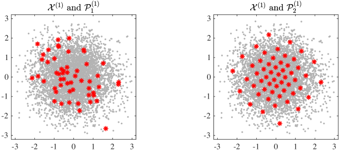
Figure 1: The scatter plots of the original binormal data ${\mathcal{X}}$ (grey points), the subsampled ${\mathcal{P}}_{1}$ and ${\mathcal{P}}_{2}$ (red asterisks). Upper: independent components; Lower: correlated components.

Let us give a toy example to illustrate that the proposed GEFD is reasonable to measure the representation of a small data with respect to the original big data. Suppose the original dataset ${\mathcal{X}}^{(1)}=\{{\mbox{\boldmath$x$}}_{i}^{(1)},i=1,\dots,N\}$ are generated from a binormal distribution with independent components, shown as the background grey points in Figure 1 (upper panel). We obtain ${\mathcal{P}}_{1}^{(1)}=\{\bm{\xi}_{k}^{(1,1)},k=1,\dots,n\}\subset{\mathcal{X}}^{(1)}$ by the URS method, and ${\mathcal{P}}_{2}^{(1)}=\{\bm{\xi}_{k}^{(1,2)},k=1,\dots,n\}\subset{\mathcal{X}}^{(1)}$ by the subsampling method in Section 4. Let us choose the kernel function ${\mathbb{K}}^{\text{M}}$ of mixture discrepancy in (2). According to the analytical expression (5), it can be obtained that

$$D^{2}({\mathcal{P}}_{1}^{(1)};{\mathcal{X}}^{(1)},{\mathbb{K}}^{\text{M}})=1.1212\times 10^{-2}>4.0424\times 10^{-4}=D^{2}({\mathcal{P}}_{2}^{(1)};{\mathcal{X}}^{(1)},{\mathbb{K}}^{\text{M}}).$$

Thus ${\mathcal{P}}_{2}^{(1)}$ is better than ${\mathcal{P}}_{1}^{(1)}$ by the criterion of GEFD. This comparison is in accordance with the observed fact in Figure 1 (upper panel), where ${\mathcal{P}}_{2}^{(1)}$ represents the full data ${\mathcal{X}}$ better than ${\mathcal{P}}_{1}^{(1)}$ does. Meanwhile, it is worthy mentioning that the GEFD by Definition 1 is also well-defined when the components of ${\mathcal{X}}$ are correlated, although the transformation $T_{{\mathcal{X}}}$ in (3) translates each coordinate of ${\mathcal{X}}$ into $[0,1]$ independently. The right hand side of (4) is a norm of the function $F_{{\mathcal{X}}}-F_{{\mathcal{P}}}$, where the ECDF $F_{{\mathcal{X}}}$ is general enough to cover any joint distributions of ${\mathcal{X}}$. For illustration, we give another example where the two components of ${\mathcal{X}}^{(2)}$ are correlated, see Figure 1 (lower panel). We obtain two different subsamples ${\mathcal{P}}_{1}^{(2)}$ and ${\mathcal{P}}_{2}^{(2)}$ respectively by the URS method and the subsampling method in Section 4, and calculate their GEFD criteria,

$$D^{2}({\mathcal{P}}_{1}^{(2)};{\mathcal{X}}^{(2)},{\mathbb{K}}^{\text{M}})=7.7165\times 10^{-3}>1.2544\times 10^{-3}=D^{2}({\mathcal{P}}_{2}^{(2)};{\mathcal{X}}^{(2)},{\mathbb{K}}^{\text{M}}).$$

It is implied that ${\mathcal{P}}_{2}^{(2)}$ is better than ${\mathcal{P}}_{1}^{(2)}$ for representing the full data, which agrees with the intuitive fact in Figure 1 (lower panel). Therefore, the GEFD is a reasonable goodness measure for a small subdata in representing the original full data.

3 Properties of the GEFD

When $N\rightarrow\infty$, the ECDF $F_{{\mathcal{X}}}({\mbox{\boldmath$x$}})$ of ${\mathcal{X}}$ converges to the CDF $F({\mbox{\boldmath$x$}})$ for ${\mbox{\boldmath$x$}}\in{\mathbb{R}}^{s}$, and the marginal ECDF $F_{{\mathcal{X}}_{(j)}}(x_{j})$ of the $j$th component converges to the $j$th marginal CDF of $F({\mbox{\boldmath$x$}})$ for $j=1,\dots,s$. Under the joint independence condition, we can derive the asymptotic equivalence between the GEFD defined in (4) and the generalized $\ell_{2}$-discrepancy in (2) upon the transformation $T_{{\mathcal{X}}}$ in (3).

Theorem 1.

Given a reference data ${\mathcal{X}}\subset{\mathbb{R}}^{s}$ satisfying the joint independence

$$F_{{\mathcal{X}}}({\mbox{\boldmath$x$}})=\prod_{j=1}^{s}F_{{\mathcal{X}}_{(j)}}(x_{j}),\quad\forall~{}{\mbox{\boldmath$x$}}=(x_{1},\dots,x_{s})^{T}\in{\mathbb{R}}^{s},$$ (6)

suppose the number of repeated points within ${\mathcal{X}}$ be upper bounded by a constant $c_{1}$, and the kernel ${\mathbb{K}}(u,v)=\prod_{j=1}^{s}K(u_{j},v_{j})$ be Lipschitz continuous in the sense of $|K(u_{1},v)-K(u_{2},v)|\leq c_{2}|u_{1}-u_{2}|,$ for any $u_{1},u_{2},v\in[0,1]$, and a constant $c_{2}$. Then for any small size data ${\mathcal{P}}\subset{\mathbb{R}}^{s}$,

$$D^{2}({\mathcal{P}};{\mathcal{X}},{\mathbb{K}})=D^{2}(T_{{\mathcal{X}}}({\mathcal{P}});F_{\rm u},{\mathbb{K}})+O(1/N^{*}),$$

where $N^{*}=min_{j\in\{1:s\}}N_{j}$ and $N_{j}$ is the number of marginal distinct values ${\mathcal{X}}_{(j)}=\{x_{ij},i=1,\dots,N\}$ along the $j$th coordinate.

For the commonly used kernel functions in (2), the Lipschitz continuous condition is easily satisfied. Theorem 1 translates the GEFD of ${\mathcal{P}}$ in ${\mathbb{R}}^{s}$ to the generalized $\ell_{2}$-discrepancy of $T_{{\mathcal{X}}}({\mathcal{P}})$ in $C^{s}$, subject to an approximation error of order $O(1/N^{*})$. For ${\mathcal{X}}$ with large sample size $N$, the quantity $N^{*}$ is also large as each continuous coordinate may entertain infinitely many distinct values. Specifically for the one-dimensional case, we obtain the following asymptotic optimality result since the equidistant point set $\{1/(2n),3/(2n),\dots,(2n-1)/(2n)\}$ is known to have the lowest discrepancy for the kernels in (2); see Zhou et al. [23].

Corollary 1.

For ${\mathcal{X}}\subset{\mathbb{R}}$ with sample size $N$ , the point set ${\mathcal{P}}$ given by

$$\bm{\xi}_{k}=F_{{\mathcal{X}}}^{-1}\left(\frac{2k-1}{2k}\right),\quad k=1,\dots,n,$$

is asymptotically optimal (as $N\rightarrow\infty$) with respect to the GEFD using the kernel function ${\mathbb{K}}^{\mathrm{C}}$, ${\mathbb{K}}^{\mathrm{W}}$ or ${\mathbb{K}}^{\mathrm{M}}$ defined in (2). Here $F_{{\mathcal{X}}}$ is the ECDF of ${\mathcal{X}}$.

Hickernell [8] pointed out an important property of the generalized $\ell_{2}$-discrepancy, known as the famous Koksma-Hlawka Inequality. Let ${\mathcal{D}}=\{\bm{\zeta}_{k},k=1,\dots,n\}$ be a set of points on $C^{s}$, and $f$ be a function on $C^{s}$, then the upper bound of the difference between the integral of $f$ over $C^{s}$ and the averaged value of $f$ among ${\mathcal{D}}$ is given by

$$\left|\int_{C^{s}}f({\mbox{\boldmath$u$}})\mbox{d}{\mbox{\boldmath$u$}}-\frac{1}{n}\sum_{k=1}^{n}f(\bm{\zeta}_{k})\right|\leq D({\mathcal{D}};F_{\mathrm{u}},{\mathbb{K}})V_{2}(f,{\mathbb{K}}),$$ (7)

where $V_{2}(f,{\mathbb{K}})$ is the generalized $\ell_{2}$-variation defined in [8]. Such Koksma-Hlawka inequality is an important result in numerical integration and quasi-Monte Carlo methods. Given the function $f$ and a reproducing kernel ${\mathbb{K}}$, $V_{2}(f,{\mathbb{K}})$ is a fixed quantity. When $V_{2}(f,{\mathbb{K}})$ is bounded in $C^{s}$, the lower the generalized $\ell_{2}$-discrepancy $D({\mathcal{D}};F_{\mathrm{u}},{\mathbb{K}})$, the smaller the upper bound in (7).

Now consider the difference between the averaged values of $f$ under two data sets. Given an $N$-size data set ${\mathcal{E}}=\{{\mbox{\boldmath$u$}}_{i},i=1,\dots,N\}\subset C^{s}$, an $n$-size data set ${\mathcal{D}}=\{\bm{\zeta}_{k},k=1,\dots,n\}\subset C^{s}$, and a reproducing kernel ${\mathbb{K}}$ on $C^{s}\times C^{s}$, write

$$D_{{\mathbb{K}}}^{2}({\mathcal{E}},{\mathcal{D}})= \int_{C^{2s}}{\mathbb{K}}({\mbox{\boldmath$u$}},{\mbox{\boldmath$v$}})\mbox{d}(F_{{\mathcal{E}}}({\mbox{\boldmath$u$}})-F_{{\mathcal{D}}}({\mbox{\boldmath$u$}}))\mbox{d}(F_{{\mathcal{E}}}({\mbox{\boldmath$v$}})-F_{{\mathcal{D}}}({\mbox{\boldmath$v$}}))$$

$$= \frac{1}{N^{2}}\sum_{i,k=1}^{N}{\mathbb{K}}({\mbox{\boldmath$u$}}_{i},{\mbox{\boldmath$u$}}_{k})-\frac{2}{Nn}\sum_{i=1}^{N}\sum_{k=1}^{n}{\mathbb{K}}({\mbox{\boldmath$u$}}_{i},\bm{\zeta}_{k})+\frac{1}{n^{2}}\sum_{i,k=1}^{n}{\mathbb{K}}(\bm{\zeta}_{i},\bm{\zeta}_{k}).$$ (8)

Here $D_{{\mathbb{K}}}^{2}({\mathcal{E}},{\mathcal{D}})$ is indeed a squared norm $\|F_{{\mathcal{D}}}-F_{{\mathcal{E}}}\|_{{\mathbb{K}}}^{2}$ induced by ${\mathbb{K}}$. When the data set ${\mathcal{E}}$ contains a large sample of points generated from the uniform distribution on $C^{s}$, $D_{{\mathbb{K}}}^{2}({\mathcal{E}},{\mathcal{D}})$ becomes the empirical form of the squared generalized $\ell_{2}$-discrepancy. In this view, $D_{{\mathbb{K}}}^{2}({\mathcal{E}},{\mathcal{D}})$ assesses the difference between ${\mathcal{E}}$ and ${\mathcal{D}}$ in terms of their empirical CDFs. Then we obtain the following lemma of the empirical form of (7) on the unit hypercube $C^{s}$.

Lemma 1 (Empirical Koksma-Hlawka Inequality on $C^{s}$).

Given two point sets ${\mathcal{E}}$, ${\mathcal{D}}\subset C^{s}$, a reproducing kernel ${\mathbb{K}}$ on $C^{s}\times C^{s}$, and the function $f$ with the bounded ${\ell}_{2}$-variation $V_{2}(f,{\mathbb{K}})$ on $C^{s}$, we have

$$\left|\frac{1}{N}\sum_{{\mbox{\boldmath$u$}}\in{\mathcal{E}}}f({\mbox{\boldmath$u$}})-\frac{1}{n}\sum_{\bm{\zeta}\in{\mathcal{D}}}f(\bm{\zeta})\right|\leq D_{{\mathbb{K}}}({\mathcal{E}},{\mathcal{D}})V_{2}(f,{\mathbb{K}}),$$

where $D_{{\mathbb{K}}}({\mathcal{E}},{\mathcal{D}})$ is given by (8).

Note that for any two data sets ${\mathcal{X}}=\{{\mbox{\boldmath$x$}}_{i},i=1,\dots,N\}\subset{\mathbb{R}}^{s}$, and ${\mathcal{P}}=\{\bm{\xi}_{k},k=1,\dots,n\}\subset{\mathbb{R}}^{s}$, through the transformation $T_{{\mathcal{X}}}$ in $(\ref{F_tra})$, it is easy to see that $T_{{\mathcal{X}}}({\mathcal{X}})\subset C^{s}$ and $T_{{\mathcal{X}}}({\mathcal{P}})\subset C^{s}$. According to the analytical expression of GEFD in (5), we have that $D^{2}({\mathcal{P}};{\mathcal{X}},{\mathbb{K}})=D_{{\mathbb{K}}}^{2}(T_{{\mathcal{X}}}({\mathcal{X}}),T_{{\mathcal{X}}}({\mathcal{P}}))$. By combining Lemma 1 and the equivalence between $D({\mathcal{P}};{\mathcal{X}},{\mathbb{K}})$ and $D_{{\mathbb{K}}}(T_{{\mathcal{X}}}({\mathcal{X}}),T_{{\mathcal{X}}}({\mathcal{P}}))$, we can deduce the empirical Koksma-Hlawka inequality in terms of GEFD defined on ${\mathbb{R}}^{s}$.

Theorem 2 (Empirical Koksma-Hlawka Inequality on ${\mathbb{R}}^{s}$).

Given a reference data ${\mathcal{X}}\subset{\mathbb{R}}^{s}$, ${\mathbb{K}}(u,v)=\prod_{j=1}^{s}K(u_{j},v_{j})$ is a reproducing kernel function on $C^{s}\times C^{s}$ and $f$ has a bounded ${\ell}_{2}$-variation $V_{2}(f,{\mathbb{K}})$ on $C^{s}$, then for any point set ${\mathcal{P}}\subset{\mathbb{R}}^{s}$,

$$\left|\frac{1}{N}\sum_{{\mbox{\boldmath$x$}}\in{\mathcal{X}}}f(T_{{\mathcal{X}}}({\mbox{\boldmath$x$}}))-\frac{1}{n}\sum_{{\mbox{\boldmath$z$}}\in{\mathcal{P}}}f(T_{{\mathcal{X}}}({\mbox{\boldmath$z$}}))\right|\leq D({\mathcal{P}};{\mathcal{X}},{\mathbb{K}})V_{2}(f,{\mathbb{K}}),$$

where $T_{{\mathcal{X}}}$ takes the form of (3), and $D({\mathcal{P}};{\mathcal{X}},{\mathbb{K}})$ is given by Definition 1.

It is worth noting that in Theorem 2 the reference data ${\mathcal{X}}$ on ${\mathbb{R}}^{s}$ is not required to satisfy the joint independence condition as in Theorem 1. Theorem 2 provides another rationale for the proposed GEFD criterion used for measuring the closeness of ${\mathcal{P}}$ to ${\mathcal{X}}$.

4 Data-driven Subsampling

Given a reference data ${\mathcal{X}}\subset{\mathbb{R}}^{s}$, we want to find a small data ${\mathcal{P}}\subset{\mathbb{R}}^{s}$ such that ${\mathcal{P}}$ has a good representation of ${\mathcal{X}}$. As discussed in the previous section, the goodness of representation can be measured by the GEFD criterion. Theorem 1 translates the GEFD of ${\mathcal{P}}\subset{\mathbb{R}}^{s}$ to the generalized $\ell_{2}$-discrepancy of $T_{{\mathcal{X}}}({\mathcal{P}})$ in $C^{s}$, subject to an approximation error of order $1/N^{*}$. Therefore, if ${\mathcal{X}}$ satisfies the joint independence assumption (6), a good design ${\mathcal{D}}$ in $C^{s}$ with low generalized $\ell_{2}$-discrepancy could lead to a point set ${\mathcal{P}}$ with low GEFD by the inverse transformation of $T_{{\mathcal{X}}}$, i.e. ${\mathcal{P}}=T_{{\mathcal{X}}}^{-1}({\mathcal{D}})$. Such inversion method can be based on an existing low-discrepancy design from the rich library of uniform experimental designs (Fang et al. [5]) or low discrepancy sequences or nets (Niederreiter [14]), whereas one may also use the R:UniDOE package (Zhang et al. [22]) for real-time construction of nearly uniform designs.

The joint independence assumption in (6) may be not satisfied for a real data set ${\mathcal{X}}\subset{\mathbb{R}}^{s}$. As a common practice, we can apply the statistical procedures such as the principal component analysis (PCA) or independent component analysis (ICA) to transform the reference data to a latent space, ${\mathcal{Z}}$. For simplicity, we suggest to use the PCA approach in this paper, which is based on the singular value decomposition (SVD), to convert the data to have linearly uncorrelated coordinates. Based on the principal scores on the latent space, one can use the inversion method to find a small representation ${\mathcal{Q}}_{{\mathcal{P}}}$ with low GEFD. Finally, such ${\mathcal{Q}}_{{\mathcal{P}}}$ can be converted back to the original space as the desired small data representation of ${\mathcal{X}}$ on ${\mathbb{R}}^{s}$.

The above procedure can be called the rotation-inversion construction, and it can be described more precisely in the following three steps: (i) performing SVD for ${\mathcal{X}}$ to obtain the rotation $V$, the singular-valued matrix $\Lambda$, and the rotated data ${\mathcal{Z}}$; (ii) constructing the data-driven space-filling design ${\mathcal{Q}}_{{\mathcal{P}}}=\{\bm{\eta}_{k},k=1,\dots,n\}$ in the space of ${\mathcal{Z}}$ by performing the $T_{{\mathcal{Z}}}^{-1}$ transformation on each $\bm{\zeta}_{k}\in{\mathcal{D}}$ as follows,

$$\bm{\eta}_{k}=T_{{\mathcal{Z}}}^{-1}(\bm{\zeta}_{k})=\big{(}F_{{\mathcal{Z}}_{(1)}}^{-1}(\zeta_{k1}),\dots,F_{{\mathcal{Z}}_{(s)}}^{-1}(\zeta_{ks})\big{)}^{T},\quad k=1,\dots,n;$$ (9)

(iii) generating the point set ${\mathcal{P}}$ by $\bm{\xi}_{k}={\mbox{\boldmath$V$}}\Lambda\bm{\eta}_{k}$ for each $k=1,\dots,n$. Such a procedure is computationally efficient for a large scale data in a low dimensional space. For an illustration, we apply the rotation-inversion construction to a two-dimensional reference data ${\mathcal{X}}$ and obtain the new sampled points ${\mathcal{P}}$, shown in Figure 2 (a) and (b). The original data ${\mathcal{X}}$ is simulated from a truncated binormal distribution with correlation, same as that in Figure 1. It can be found that such a small data ${\mathcal{P}}$ (plotted as circles) represents the original data ${\mathcal{X}}$ (plotted as dots) quite well.

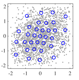
(a) Original Space

(b) Rotated Space

(c) Data-driven Subsampling

Figure 2: Data-driven space-filling design by the rotation-inversion construction method and data-driven subsampling by non-uniform stratification and nearest neighbor on the rotated space.

For the subsampling purpose, it is required that the obtained small data ${\mathcal{P}}$ should be a subset of the original data ${\mathcal{X}}$. Since the rotated data ${\mathcal{Z}}$ is only nearly independent, there exist some points in ${\mathcal{Q}}_{{\mathcal{P}}}$ not belonging to ${\mathcal{Z}}$. For each of such data point, we suggest to find its nearest neighbor in ${\mathcal{Z}}$ as a replacement. In Figure 2 (c), the points of ${\mathcal{Q}}_{{\mathcal{P}}}$ are shown as the circle points, and their nearest points from ${\mathcal{Z}}$ are shown as the star points. To find the nearest neighbor of each point in ${\mathcal{Q}}_{{\mathcal{P}}}\backslash{\mathcal{Z}}$, KD-tree is the conventional methods. However, the time complexity of constructing a KD-tree is $\mathcal{O}\left(PN\log N\right)$, the time complexity of searching the nearest neighbor for a design point is $\mathcal{O}\left(N^{\left(p-1\right)/p}\right)$. This can be very time consuming when the sample size N is very large, which is common in the big data era. Therefore, KD-tree cannot be applied to this case directly, it is critical to develop an effective subdata selection algorithm.

One way is to limit the search space for each point in ${\mathcal{Q}}_{{\mathcal{P}}}\backslash{\mathcal{Z}}$. We introduce a non-uniform stratification into the search step. Given the size of subdata $n$, by the following transformation for every coordinate $j$,

$$\kappa_{kj}=F_{{\mathcal{Z}}_{(j)}}^{-1}(k/n),~{}k=1,\dots,n-1,$$ (10)

so each coordinate of the rotated space is divided into $n$ partitions. It is approximately balanced when each partition has $\lfloor N/n\rfloor$ or $\lceil N/n\rceil$ points. In fact, in (10), the obtained $\kappa_{1j},\dots,\kappa_{n-1,j}$ are the quantiles of ${\mathcal{Z}}_{(j)}$. Denote $\kappa_{0j}=\min{\mathcal{Z}}_{(j)}$, $\kappa_{nj}=\max{\mathcal{Z}}_{(j)}$, and the $k$th partition as $\big{(}\kappa_{k-1,j},\kappa_{kj}\big{]}$ for $k=1,\dots,n$. Then any value $z\in[\kappa_{0j},\kappa_{nj}]$ locates in the partition marked with $\lceil nF_{{\mathcal{Z}}_{(j)}}(z)\rceil$. Conversely, any $\zeta\in[0,1]$ can be converted into a value belonging to the $(\lceil n\zeta\rceil)$th partition of $[\kappa_{0j},\kappa_{nj}]$. These cuts in the $s$ coordinates altogether define a non-uniform stratification grid of the rotated space. See Figure 2 (c) for such non-uniform grid (formed by the dotted lines). The whole rotated space is divided into the $n^{s}$ different cells within the grids. Label each cell with an $s$-dimensional index vector to distinguish different cells. It is easy to justify that any point ${\mbox{\boldmath$z$}}=(z_{1},\dots,z_{s})^{T}$ in the rotated space is located in the cell indexed by $(\lceil nF_{{\mathcal{Z}}_{(1)}}(z_{1})\rceil,\cdots,\lceil nF_{{\mathcal{Z}}_{(s)}}(z_{s})\rceil)^{T}$, which helps to locate $z$ in this non-uniform stratification. To this end, for each ${\mbox{\boldmath$z$}}_{i}$ in ${\mathcal{Z}}$ we find its cell index vector $I_{i}=(\lceil nF_{{\mathcal{Z}}_{(1)}}(z_{i1})\rceil,\cdots,\lceil nF_{{\mathcal{Z}}_{(s)}}(z_{is})\rceil)^{T}$.

Algorithm 1 Data-driven Subsampling

0:  The original data ${\mathcal{X}}=\{{\mbox{\boldmath$x$}}_{1},\dots,{\mbox{\boldmath$x$}}_{N}\}\subset{\mathbb{R}}^{s}$, the neighboring radius $\tau$ and a uniform design ${\mathcal{D}}=\{\bm{\zeta}_{1},\dots,\bm{\zeta}_{n}\}\subset C^{s}$.

1:   Perform SVD ${\mathcal{X}}={\mathcal{Z}}\Lambda{\mbox{\boldmath$V$}}^{T}$ for ${\mathcal{X}}$ to obtain the rotated data ${\mathcal{Z}}=\{{\mbox{\boldmath$z$}}_{1},\dots,{\mbox{\boldmath$z$}}_{N}\}$ whose components are linearly uncorrelated;

2:   Implement non-uniform stratification to the rotated space, and label the $n^{s}$ cells with the corresponding index vectors. Then for each $i=1,\dots,N$, the point ${\mbox{\boldmath$z$}}_{i}=(z_{i1},\dots,z_{is})^{T}\in{\mathcal{Z}}$ falls into the cell with index vector $I_{i}=(\lceil nF_{{\mathcal{Z}}_{(1)}}(z_{i1})\rceil,\cdots,\lceil nF_{{\mathcal{Z}}_{(s)}}(z_{is})\rceil)^{T};$

3:   Apply the inverse transformation (9) on the uniform design ${\mathcal{D}}$ to obtain the data-driven space-filling design ${\mathcal{Q}}_{{\mathcal{P}}}=\{\bm{\eta}_{1},\dots,\bm{\eta}_{n}\}$ in the rotated space. Then for each $k=1,\dots,n$, the design point $\bm{\eta}_{k}=T_{{\mathcal{Z}}}^{-1}(\bm{\zeta}_{k})=\big{(}F_{{\mathcal{Z}}_{(1)}}^{-1}(\zeta_{k1}),\dots,F_{{\mathcal{Z}}_{(s)}}^{-1}(\zeta_{ks})\big{)}^{T}$ is located in the cell with index vector $J_{k}=(\lceil n\zeta_{k1}\rceil,\cdots,\lceil n\zeta_{ks}\rceil)^{T};$

4:   For each $\bm{\eta}_{k}$, identify the points located in $\bm{\eta}_{k}$’s neighboring cells with their index vectors in the range of $\tau$ from $J_{k}$ in the version of ${\ell}_{\infty}$-norm, and find out the nearest sample index $i_{k}^{*}$, i.e. $i_{k}^{*}=\min_{\left\{i:~{}\parallel I_{i}-J_{k}\parallel_{\infty}\leq\tau\right\}}\parallel{\mbox{\boldmath$z$}}_{i}-\bm{\eta}_{k}\parallel_{2},\quad k=1,\dots,n.$

4:  Data-driven subsample ${\mathcal{P}}^{\dagger}=\{{\mbox{\boldmath$x$}}_{i_{1}^{*}},\dots,{\mbox{\boldmath$x$}}_{i_{n}^{*}}\}$.

For an $n$-level uniform design ${\mathcal{D}}=\{\bm{\zeta}_{k},k=1,\dots,n\}$ in $C^{s}$, all its entries locate at the center of the bins of $(0,1/n],\dots,((n-1)/n,1]$. By using ${\mathcal{D}}$ to construct ${\mathcal{Q}}_{{\mathcal{P}}}$, each $\bm{\eta}_{k}=T_{{\mathcal{Z}}}^{-1}(\bm{\zeta}_{k})=\big{(}F_{{\mathcal{Z}}_{(1)}}^{-1}(\zeta_{k1}),\dots,F_{{\mathcal{Z}}_{(s)}}^{-1}(\zeta_{ks})\big{)}^{T}$ is located in one and only one of the $n^{s}$ cells. Denote this cell by Cell_k, and its index vector by $J_{k}$. Obviously $J_{k}=(\lceil n\zeta_{k1}\rceil,\dots,\lceil n\zeta_{ks}\rceil)^{T}$ according to the process of labeling the index vector for a cell. Meanwhile, $\bm{\eta}_{k}$ is also labeled by $J_{k}$. Then we can find a sampling point indexed by $i_{k}^{*}$ from $\{i:{\mbox{\boldmath$z$}}_{i}\in\mathrm{Cell}_{k}\cap{\mathcal{Z}}\}$ that is nearest to $\bm{\eta}_{k}$. Note that when the condition of the joint independence (6) is not satisfied, there could exist cells consisting none of points from ${\mathcal{Z}}$. Then search region may be increased to the neighboring cells around $\bm{\eta}_{k}$. Since the non-uniform stratification in (10) is carried out component by component independently, each neighboring cell is determined by a radius $\tau$ in the meaning of ${\ell}_{\infty}$-norm of the difference between its index vector $J$ and $J_{k}$. It is equivalent to that the $J$ is satisfied with $||J_{k}-J||_{\infty}\leq\tau$. Then the points to be searched are locating in the cells with index vectors belonging to the $s$-dimensional rectangular $\big{[}\lceil n\zeta_{k1}\rceil-\tau,\lceil n\zeta_{k1}\rceil+\tau\big{]}\otimes\dots\otimes\big{[}\lceil n\zeta_{ks}\rceil-\tau,\lceil n\zeta_{ks}\rceil+\tau\big{]}$. Therefore, there is always a nearest neighboring sample from ${\mathcal{Z}}$ that can be found for each $\bm{\eta}_{k}$.

We summarize the above procedure by Algorithm 1. As an example, it can output the subsampled points shown in Figure 2 (c). For each design point (circle points) in the rotated space, a corresponding sample (star annotation) is found from ${\mathcal{Z}}$, which is closest the ideal design point. It is anticipated that such kind of subdata ${\mathcal{P}}^{\dagger}$ is similar to the designed ${\mathcal{P}}$ and has low GEFD value.

5 Accelerated Subsampling Procedure

In this section, we present an approximate approach to speed up the subsampling algorithm, which is useful for the implementation in high-dimensional cases. A parallel scheme based on sliced uniform designs is provided to deal with the complex situation where the storage of the original full data is decentralized by multiple servers.

Note that the essence of Algorithm 1 is to partition the rotation space into $n^{s}$ intensive cells firstly, and to conduct the nearest searching process in the neighboring cells dynamically determined by each point in $T_{{\mathcal{Z}}}^{-1}({\mathcal{D}})$ with a certain radius $\tau$ in the meaning of ${\ell}_{\infty}$-norm. For the high dimensional case, the whole space is divided into the $n^{s}$ cells, and a relatively large radius $\tau$ is needed to guarantee the union of neighboring cells is nonempty. However if $\tau$ is too large, it is still very time consuming to identify the points that belong to the target neighboring cells and further to search for the nearest sample index from the original data. Moreover, it is not easy to find an appropriate radius to determine the neighboring cells.

An alternative stratification strategy is to use a gross grid in the starting step. For each coordinate $j$, we divide the $j$th coordinate of the rotated space into the $m$ partitions with the nodes $\{F_{{\mathcal{Z}}_{(j)}}^{-1}(1/m),\dots,F_{{\mathcal{Z}}_{(j)}}^{-1}((m-1)/m)\}$ such that each partition has the $\lfloor N/m\rfloor$ or $\lceil N/m\rceil$ points. Then the whole space is divided into the $m^{s}$ blocks. Each block is labeled with a unique code in lexicographic order. Then each point in ${\mathcal{Z}}$ can be labeled by the code of the block which the point belongs to. In this way, all the points are divided into at most the $m^{s}$ groups by their block codes. For each $\bm{\eta}_{k}\in T_{{\mathcal{Z}}}^{-1}({\mathcal{D}})$, there is one and only one of the blocks with block code $C_{k}\in\{1,\dots,m^{s}\}$ containing $\bm{\eta}_{k}$ and the search space is narrowed to one of the $m^{s}$ blocks which consists of all the points with the same block code $C_{k}$. The computational complexity of searching for a required code number among $N$ codes is much lower than that of searching for several different satisfied $s$-dimensional index vectors from $N$ cell index vectors, especially when $N$ is huge and $s$ is large. It implies that the process of identifying the points labeled by their block codes accelerates Step 4 in Algorithm 1 in the high-dimensional cases. We call this procedure the accelerated data-driven subsampling (ADDS) method.

Compared with the DDS algorithm, ADDS adapts to a more gross non-uniform stratification. This stratification strategy uses no information about $T_{{\mathcal{Z}}}^{-1}({\mathcal{D}})$. Moreover, since the labeling method is based a block code rather than an $s$-dimensional cell index vector, it accelerates the speed of nearest search process. See Algorithm 2 for the concrete procedure of ADDS.

Algorithm 2 Accelerated Data-driven Subsampling

0:  The original data ${\mathcal{X}}\subset{\mathbb{R}}^{s}$, a block parameter $m$ and a uniform design ${\mathcal{D}}=\{\bm{\zeta}_{k},k=1,\dots,n\}\subset C^{s}$.

1:  Perform SVD ${\mathcal{X}}={\mathcal{Z}}\Lambda{\mbox{\boldmath$V$}}^{T}$;

2:  Parallel for each point ${\mbox{\boldmath$z$}}_{i}=(z_{i1},\dots,z_{is})^{T}\in{\mathcal{Z}}$, label its block code in lexicographic order as

$$S_{i}=(\lceil mF_{{\mathcal{Z}}_{(1)}}(z_{i1})\rceil-1,\cdots,\lceil mF_{{\mathcal{Z}}_{(s)}}(z_{is})\rceil-1)\cdot(m^{s-1},\dots,m^{0})^{T}+1,~{}~{}i=1,\dots,N.$$

3:  Parallel for each $\bm{\eta}_{k}=T_{{\mathcal{Z}}}^{-1}(\bm{\zeta}_{k})$ in $T_{{\mathcal{Z}}}^{-1}({\mathcal{D}})$, label its block code in lexicographic order as

$$C_{k}=(\lceil m\zeta_{k1}\rceil-1,\cdots,\lceil m\zeta_{ks}\rceil-1)\cdot(m^{s-1},\dots,m^{0})^{T}+1,~{}~{}k=1,\dots,n.$$

4:  Parallel for each $\bm{\eta}_{k}\in T_{{\mathcal{Z}}}^{-1}({\mathcal{D}})$, find the nearest sample index $i_{k}^{**}$ from those sharing the same block code, i.e. $\{i:S_{i}=C_{k}\}$.

4:  Data-driven subsample ${\mathcal{P}}^{\dagger\dagger}=\{{\mbox{\boldmath$x$}}_{i^{**}},k=1,\dots,n\}$.

Remark 1.

For the block parameter $m$, a small integer is enough especially when the dimension of ${\mathcal{Z}}$ is high ($m=2$ or $3$ is enough for the high dimensional case). Thus for each $\bm{\eta}_{k}$, its subordinate block is usually nonempty. If unfortunately, a slightly bigger $m$ causes that some $\bm{\eta}_{k_{0}}$ locates in an empty block, we could conduct the nearest searching step among at most $2m$ closest blocks with the block codes $C_{k_{0}}\pm m^{s-1},\dots,C_{k_{0}}\pm m^{0}$. Then the nearest searching step for $\bm{\eta}_{k_{0}}$ in Algorithm 2 can be modified as “find the nearest sample index $i_{k_{0}}^{**}$ from $\{i:S_{i}\in\{C_{k_{0}}\pm m^{s-1},\dots,C_{k_{0}}\pm m^{0}\}\}$”.

Now we present the difference between the DDS and ADDS on the nearest searching step through a simple case of $s=2$. ${\mathcal{D}}=\{(1/8,5/8),(3/8,1/8),(5/8,7/8),(7/8,3/8)\}$ is a $4$-run uniform design in $C^{2}$. Assume the whole space ${\mathcal{Z}}$ consists of the black points in Figure 3. Then the data-driven space-filling design $T_{{\mathcal{Z}}}^{-1}({\mathcal{D}})$ based on ${\mathcal{D}}$ is the set of circle points in Figure 3. Consider the point with notation “3” in $T_{{\mathcal{Z}}}^{-1}({\mathcal{D}})$ as an example to show the different searching scopes for the DDS and ADDS. For the DDS, each coordinate of ${\mathcal{Z}}$ is divided into $4$ partitions by the dotted lines, see Figure 3 (a). The point “3” is located in the cell with index vector $(3,4)^{T}$. But this cell does not contain any point of ${\mathcal{Z}}$. Then a radius $\tau=1$ is set and the neighboring cells to be searched have the index vector $(id_{1},id_{2})^{T}$ satisfying $\max\left\{\left|id_{1}-3\right|,\left|id_{2}-4\right|\right\}\leq 1$. Thus the nearest search process is implemented among the black points in the rectangle bounded by solid lines. For the ADDS with $m=3$, the corresponding nearest search scope is the block that contains the point “3”, i.e. the rectangle bounded by solid lines in Figure 3 (b). If a bigger $m=4$ is implied, i.e. the same non-uniform stratification with that in DDS, the block containing the point “3” contains none of points of ${\mathcal{Z}}$, according to the modification recommended in Remark 1, the nearest search scope for this point is the union of the points contained in the three rectangles bounded by solid lines in Figure 3 (c). The final searched subdata sets are the star points in each subfigure of Figure 3. In these example, the three searched subdata sets contain the same points of ${\mathcal{Z}}$. Note that the KD-tree algorithm can be applied to search the nearest sample index sharing the same block code. We can constructed a KD-tree for each block generated by ADDS with time complexity to be $\mathcal{O}\left(P\left(N/m^{p}\right)\log\left(N/m^{p}\right)\right)$ and search a nearest neighbour from the design with time complexity to be $\mathcal{O}\left(P\left(N/m^{p}\right)^{\left(p-1\right)/p}\right)$.

(a) DDS with $\tau=1$

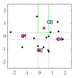
(b) ADDS with $m=3$

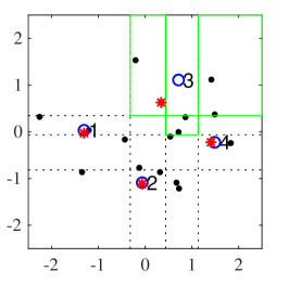
(c) ADDS with $m=4$

Figure 3: An simple example to illustrate the difference between DDS and ADDS. The dotted lines give the non-uniform stratification for each coordinate; The rectangles bounded by solid lines in (a), (b) and (c) are respectively the nearest search scopes for the point “3” in DDS with the radius $\tau=1$, and ADDS with the block parameter $m=3$ and $4$, respectively; The star points in each subfigure are the corresponding obtained subdata.

To further certify the performance of ADDS intuitively, we consider the case of $s=10$, where the full data set ${\mathcal{X}}$ is randomly generated from the $s$-dimensional uniform distribution with independent components each on [0,1]. Let the data size $N=10^{4},10^{5}$,$10^{6}$ and $10^{7}$, respectively. Consider the data-driven subsampling procedure with $\tau=750,550,400$ and $300$ respectively for the different $N$ according to Algorithm 1, and the ADDS procedure with block parameters $m=2$, to obtain subsamples with size $n=2000$. Table 1 shows the computing time for each $N$ carried out on a server Intel(R) Xeon(R) with CPU E5-2650 v4 and 2.20 GHz. It can be seen that the accelerated approach significantly speeds up the subsampling procedure.

Table 1: CPU seconds with $n=2000$, $s=10$ and different full data size $N$.

Method	$N$
	$10^{4}$	$10^{5}$	$10^{6}$	$10^{7}$
DDS	0.2668	1.2329	11.4039	143.5468
ADDS	0.0998	0.2930	2.6088	27.6287

In practical application, we may encounter more complex situation where the storage of the initial data decentralizes in different servers because of memory constraint. In this case, it is difficult to obtain a subdata having good presentation with respect to this type of decentralized initial data. It seems impractical to combine the decentralized parts of the full data together to apply the DDS or ADDS based on a general uniform design directly. To deal with this problem, we use the idea of divide-and-conquer. Assume the initial data contains ${L}$ decentralized parts with the size of $N_{(1)},\dots,N_{({L})}$, and the size of subdata sets to be subsampled from ${L}$ parts are $n_{(1)},\dots,n_{({L})}$ according to the proportion of $N_{(1)},\dots,N_{({L})}$. The ${L}$ decentralized parts can be seen as the ${L}$ resulting parts of the objectively dividing of the whole initial data. Then treat every part as the full data in Algorithm 1 or 2 to perform the DDS or ADDS. Finally combining the ${L}$ obtained subdata sets from the ${L}$ parts acquires the subsample of the initial data. The $n_{(1)}$-, $\dots,n_{({L})}$-run small uniform designs used as the input terms in DDS or ADDS have the following inherent connections:

(i)

The combination of the ${L}$ designs is an $n$-level sliced uniform design ${\mathcal{D}}$ on $C^{s}$;

(ii)

for each $l=1,\dots,{L}$, the $\left(\sum_{k=1}^{l}n_{(k-1)}+1\right)$th to $\left(\sum_{k=1}^{l}n_{(k)}\right)$th run of ${\mathcal{D}}$ corresponds to the $n_{(l)}$-run small uniform design ${\mathcal{D}}_{(l)}$ used for performing DDS or ADDS for the $l$th parts;

(iii)

for each $j=1,\dots,s$ and $l=1,\dots,{L}$, the $n_{l}$ entries of the $j$th factor in ${\mathcal{D}}_{(l)}$ have exactly one element in each of the $n_{(l)}$ bins of $\left(0,1/n_{(l)}\right],\dots,\left((n_{(l)}-1)/n_{(l)},1\right]$.

Here, $n=n_{1}+\cdots+n_{{L}}$, and a sliced uniform design is the uniform design ${\mathcal{D}}$ that can be partitioned into some slices ${\mathcal{D}}_{(l)},l=1,\dots,{L},$ and each slice has good uniformity. For measuring the uniformity of such a design, Chen et al. [3] used the combined centered ${\ell}_{2}$-discrepancy to measure the uniformity of the sliced Latin hypercube designs where each slice has the same size. Yuan et al. [21] used a weighted average centered ${\ell}_{2}$-discrepancy to obtain uniform flexible sliced Latin hypercube designs of which the slices may have different run sizes. Since the mixture discrepancy is better than the centered ${\ell}_{2}$-discrepancy, we use the following weighted average mixture discrepancy

$${\rm WAMD}({\mathcal{D}})=\frac{1}{2}D({\mathcal{D}};F_{\rm u},{\mathbb{K}}^{M})+\sum_{l=1}^{\ell}\frac{n_{(l)}}{2n}D({\mathcal{D}}_{(l)};F_{\rm u},{\mathbb{K}}^{M})$$

to measure the uniformity of the sliced uniform designs. Both the flexible sliced Latin hypercube designs by Yuan et al. [21] and the sliced Latin hypercube designs with arbitrary run sizes by Xu et al. [20] satisfy the above connection (iii). The connections (i) and (ii) are reflected from the combined uniformity of the ${\mathcal{D}}$ and ${\mathcal{D}}_{(l)},l=1,\dots,\ell.$ Then, the sliced uniform designs can be obtained by the optimization algorithm under the weighted average mixture discrepancy criterion. Given a sliced uniform design, we assign each slice to the corresponding part of the initial data, and conduct the DDS or ADDS in parallel to obtain the corresponding subdata of each part. The final subsample obtained through the DDS or ADDS based on the sliced uniform design is the union of these subdata sets.

6 Numerical Examples

In this section, we show the model-free property of the subsampling method through both simulation data and a real case study. When using Algorithm 1, we only select the leading components that give no less than 85% of variance explained in the rotated space. This operation yields a lower dimensional rotated pace, and reduces the computational burden due to non-important components.

For the given subsample size $n$, and the determined dimension of the rotated pace $s$, the $n$-run $s$-factor uniform design in Algorithm 1 is constructed by the leave-one-out good lattice point method with power generator. In this construction method, the generator vector is given by a positive integer $\alpha$ which satisfies that the great common divisor of $n+1$ and $\alpha$ is one and $\alpha,\alpha^{2},\dots,\alpha^{s}$ are distinct. Then for each $j=1,\dots,s-1$, the remainders after dividing $\alpha^{j},2\alpha^{j},\dots,n\alpha^{j}$ by $n+1$ are $n$ distinct integers. Denote this generator vector by $\gamma_{\alpha}$, and it has a power form $(\alpha^{0},\alpha^{1},\dots,\alpha^{s-1})$. Then the corresponding design generated by $\gamma_{\alpha}$ is ${\mathcal{D}}^{(\alpha)}=\{\bm{\zeta}_{i}^{(\alpha)},i=1,\dots,n\}$, where $\bm{\zeta}_{i}^{(\alpha)}=\mathrm{mod}\left(i\gamma_{\alpha},n+1\right)/n-1/(2n)$ with $\mathrm{mod}\left(\cdot,\cdot\right)$ denoted as the modulus operation. Different values of $\alpha$ lead to different designs. We use the mixture discrepancy as the uniformity criterion. Finally, the uniform design ${\mathcal{D}}$ constructed by the leave-one-out good lattice point method with power generator is the one which owes the smallest mixture discrepancy value among all possible ${\mathcal{D}}^{(\alpha)}$. This construction procedure provides a fast and effective method for selecting the $n$ design points from $n^{s}$ lattice points. The designs constructed by the leave-one-out good lattice point method with power generator are indeed approximate uniform designs. For comparison, another simplest model-free subsampling method URS is also implemented. To make the different subsampling methods comparable, for each given subsample size $n$, the implementation of URS is executed for $R$ repetitions to obtain the mean, median and bounds of the results of the URS’s subsample. Moreover we use a random shift of $\varepsilon\in C^{s}$ for all design points in ${\mathcal{D}}=\{\bm{\zeta}_{k},k=1,\dots,n\}$, to obtain another approximate uniform design ${\mathcal{D}}_{\varepsilon}=\{\mathrm{mod}(\bm{\zeta}_{k}+\varepsilon,1),k=1,\dots,n\}$. Performing this random shift for $R$ repetitions results $R$ approximate uniform designs. Then we also obtain the mean, median and bounds of the results corresponding to DDS.

6.1 Simulation Studies

In this subsection, we utilize the data-driven subsampling method for both classification and regression problems. For each kind of model, we compare the prediction property of the trained models based on the subdata sets by different subsampling strategies. It will be shown that the proposed DDS method possesses the model-free property, and outperforms URS method in various settings.

In each simulation,we generate two $N$-size data sets respectively as the full data ${\mathcal{X}}_{\text{Full}}$ and the test data ${\mathcal{X}}_{\text{Test}}$ through the same generation way as well as the corresponding binary class label (and response in regression problem) ${\mathcal{Y}}_{\text{Full}}$ and ${\mathcal{Y}}_{\text{Test}}$. To measure the prediction performance of a specified type of model trained upon the $n$-size subdata ${\mathcal{P}}$ from ${\mathcal{X}}_{\text{Full}}$, we fit a corresponding model using ${\mathcal{P}}$ to predict the class label (or response) for each point in ${\mathcal{X}}_{\text{Test}}$. Denote the fitted model by $\hat{h}(\cdot)$. For each ${\mbox{\boldmath$x$}}\in{\mathcal{X}}_{\text{Test}}$, the corresponding predicted class label (or response) is $\hat{h}({\mbox{\boldmath$x$}})$. Then a prediction error could be computed by $\epsilon=\frac{1}{N}\left\|\hat{h}({\mathcal{X}}_{\text{Test}})-{\mathcal{Y}}_{\text{Test}}\right\|_{2}^{2}$ which represents the misclassification rate for the classification problem with class labels being $0$ or $1$, and mean squared prediction error in the regression case, upon the test data ${\mathcal{X}}_{\text{Test}}$. Denote this criterion by Err and MSPE respectively for the classification and regression problem. The lower value of this criterion, the better of the prediction performance.

(A) Working model is true.
For the classification simulation, let $N=10^{4}$ and both the data sets ${\mathcal{X}}_{\text{Full}}$ and ${\mathcal{X}}_{\text{Test}}$ be generated from the multinormial distribution ${\mathcal{N}}(\mathbf{0},\bm{\Sigma})$, where $\bm{\Sigma}_{ij}=0.5^{I(i\neq j)}$, $i,j=1,\dots,7$. The kind of data set is also used in Wang et al. [15].

Logistic regression model is a classical and widely used classification method for its simplicity and effectiveness. Consider the logistic regression as a classification model. Fortunately, if the underlying model is the logistic model, for example, the probability of the class label being $1$ for a point $x$ is $h({\mbox{\boldmath$x$}},\bm{\beta})=1/\big{(}1+\exp(-{\mbox{\boldmath$x$}}^{T}\bm{\beta})\big{)},$ where $\bm{\beta}$ is a $7\times 1$ vector of $0.5$, the optimal subsampling methods (mMSE and mVc) in Wang et al. [15] could be adopted. Consider the four different kinds of subsampling strategies: URS, mVc, mMSE and DDS, to obtain the subdata with $n=400,550,750,950,1200$ and $1500$, respectively. The implementations of mVc and mMSE are represented by a two-step algorithm. The first step obtains $r_{0}$ points randomly, and the other $n-r_{0}$ points are obtained in the second step based on their optimal subsampling probabilities. For this type of data sets, Wang et al. [15] suggested $r_{0}=200$ to well present the good performance of mVc and mMSE. For each $n$, every subsample strategy is executed $1000$ times because of the randomness. Recall that, the randomness of DDS is reflected from the random shift for a initial constructed approximate uniform design.

Figure 4 contains the misclassification rates of the fitted logistic regression models based on the subdata sets obtained by the four methods. For comparison, the fitted logistic regression model based on ${\mathcal{X}}_{\text{Full}}$ is also considered. For each subsample size $n$, Figure 4 (a) presents the mean values of the $1000$ results for the four subsampling methods which are denoted by URS_mean, mVc_mean, mMSE_mean, and DDS_mean; Figure 4 (b) presents the median values and lower and upper bounds of the $1000$ results corresponding to the four methods which are denoted by URS_median, mVc_median, mMSE_median, DDS_median, and URS_bounds, mVc_bounds, mMSE_bounds, DDS_bounds, respectively. In the version of mean and median, Figure 4 illustrates that the mVc, mMSE and DDS all outperform URS. The subsampling methods mVc and mMSE are based on the logistic model, they have better performance than URS when the model is correct, as shown in Wang et al. [15]. The subdata sets obtained by DDS have better representation with respect to the original data than that by URS. Therefore, the better similarity of the original data helps to better fit the model. Figure 4 (b) also shows a narrower interval of DDS than URS. It means that the subdata from DDS is more robust than other methods. Moreover, the performance of DDS is as similar as that of mVc and mMSE.

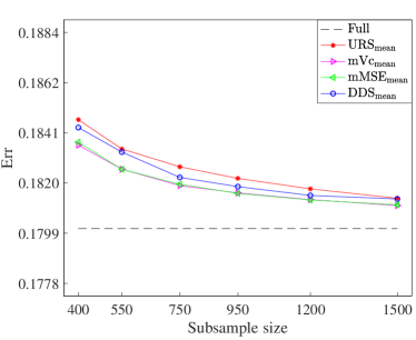
(a) Logistic Regression Classification

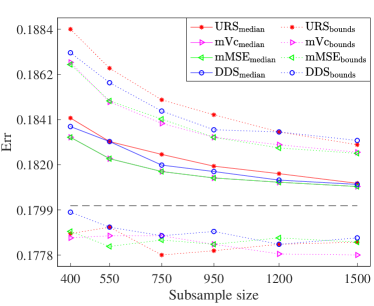
(b) Logistic Regression Classification

Figure 4: The classification errors of the fitted logistic regression model based on the subdata sets obtained by each subsampling strategy. (a): the mean values of 1000 results for each methods; (b): the median values and bounds of 1000 results for each methods.

(B) Working model is misspecified.
We evaluate the performance of different subsampling strategies while working model is misspecified. We simulate the real life borehole example of the flow rate of water through a borehole from an upper aquifer to a lower aquifer separated by an impermeable rock layer. This example was investigated by many authors such as Worley [19], Morris et al. [13], Ho and Xu [10], and Fang et al. [5]. The response variable ${\mathcal{Y}}$, the flow rate through the borehole in $m^{3}/yr$, is determined by a complex nonlinear function as follows,

$${\mathcal{Y}}=\frac{2\pi T_{\rm u}(H_{\rm u}-H_{\rm l})}{\ln(r/r_{\rm w})\left[1+\dfrac{2LT_{\rm u}}{\ln(r/r_{\rm w})r_{\rm w}^{2}K_{\rm w}^{2}}+\dfrac{T_{\rm u}}{T_{\rm l}}\right]},$$ (11)

where the $8$ input variables with their usual input ranges are listed as follows: $r_{\rm w}\in[0.05,0.15]$ means the radius of borehole ($m$); $r\in[100,50000]$ means the radius of influence ($m$); $T_{\rm u}\in[63070,115600]$ means the transmissivity of upper aquifer ($m^{2}/yr$); $T_{\rm l}\in[63.1,116]$ means the transmissivity of lower aquifer ($m^{2}/yr$); $H_{\rm u}\in[990,1110]$ means the potentiometric head of upper aquifer ($m$); $H_{\rm l}\in[700,820]$ means the potentiometric head of lower aquifer ($m$); $L\in[1120,1680]$ means the length of borehole ($m$); $K_{\rm w}\in[9855,12045]$ means the hydraulic conductivity of borehole ($m/yr$). The distribution of $r_{\rm w}$ is the normal distribution ${\mathcal{N}}(0.10,0.0161812^{2})$, the distribution of $r$ is the lognormal distribution Lognormal$(7.71,1.0056^{2})$, and the distributions of other variables are all continuous uniform distribution on their corresponding domains.

To compare the performances of different subsampling methods for the large scale data sets, let the size of the full data $N=10^{6}$, and the size of subdata $n=50,80,150,250$ and $400$, respectively. We generate the $N$-size 8-factor ${\mathcal{X}}_{\text{Full}}$ and ${\mathcal{X}}_{\text{Test}}$ for training and testing, respectively, and the corresponding responses ${\mathcal{Y}}_{\text{Full}}$ and ${\mathcal{Y}}_{\text{Test}}$ through (11). For the data $({\mathcal{X}}_{\text{Full}},{\mathcal{Y}}_{\text{Full}})$, we use different subsampling methods to obtain the subdata sets and use different models to fit each subdata set. The test data $({\mathcal{X}}_{\text{Test}},{\mathcal{Y}}_{\text{Test}})$ can be used to compare the performance of the different subsampling methods.

First, we compare URS, DDS, IBOSS, kernel herding (KH) and support points (SP) under the simple linear model. IBOSS proposed by Wang et al. [16] is a kind of optimal subsampling for linear regression model. KH proposed by Chen et al.[2] and SP proposed by Mak and Joseph[12] are two popular data-based subsampling methods. According to the generation method of ${\mathcal{X}}_{\text{Full}}$, the components of the data are mutually independent, so there do not need the rotation step in the process of DDS any more. For each subsample size $n$, URS, DDS and SP are all executed $1000$ times because of the randomness. IBOSS and KH are both executed one time. For comparison, we also fit the same model for the full data.

Figures 5 (a) and 5 (b) show the MSPE values of the fitted linear regression model based on the full data and the subdata sets with different subsample size obtained by the five subsampling methods. To present the results more explicitly, the vertical axises in 5 are logarithmically transformed. For all subsampling methods except KH, the MSPE values of the fitted models based on the subdata sets are more close to that based on full data sets as the subsampling size arises. As shown in Figure 5, the MSPE values of the DDS are much lower than that of URS especially when the subsample size $n$ is relatively small, and are close to that of the full data no matter from the version of mean or median. Moreover, DDS performs better than KH and IBOSS. In addition, Table 2 provide in Appendix B shows for most subsample size $n$, the upper bounds of the MSPE values of DDS are even lower than the MSPE values of IBOSS, KH, the mean and median MSPE values of URS. Thus the prediction ability of the fitted linear models based on the subsamples by DDS significantly outperforms that of URS, KH and IBOSS. Moreover, under the MSPE criterion, the model-based IBOSS performs worst among the three subsampling methods, which may be caused by that the simple linear model is not enough to capture the relationship between the output ${\mathcal{Y}}$ and the $8$ input variables. The MSPE values of SP is the lowest in this case because our original variables are generated by some simple distribution. SP is adept in mining such distribution from the data and using them to make prediction. If some nonlinear transformation are applied to the parameters, it will be difficult for SP to handle the data, which can be demonstrated by the following model.

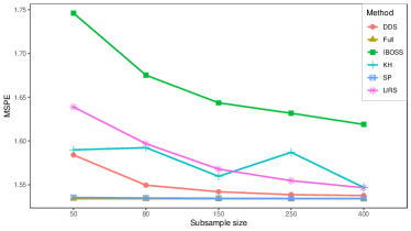
(a) Mean MSPE of Linear Regression upon the Original Data

(b) Median MSPE of Linear Regression upon the Original Data

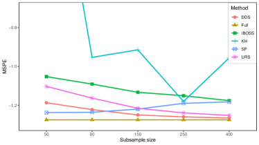
(c) Mean MSPE of Generalized Linear Regression upon the Transformed Data

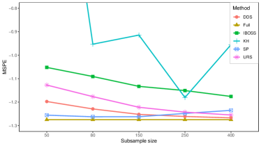
(d) Median MSPE of Generalized Linear Regression upon the Transformed Data

Figure 5: The MSPE values of the fitted linear regression model based on the subdata sets obtained through different subsample strategies from the full data sets with the original form and the transformed form for the borehole experiments.

To compare the robustness of the sampling methods, we consider generalized regression models. A careful study by Ho and Xu [10] suggested fitting $\log({\mathcal{Y}})$ with $10$ terms: $\log(r_{\rm w})$, $\log(r)$, $H_{\rm u}$, $H_{\rm l}$, $L$, $K_{\rm w}$, $H_{\rm u}*H_{\rm l}$, $H_{\rm u}^{2}$, $H_{\rm l}^{2}$ and $L^{2}$. In the generalized linear regression model, there are only $6$ significant variables: $r_{\rm w}$, $r$, $H_{\rm u}$, $H_{\rm l}$, $L$ and $K_{\rm w}$. Then the DDS is executed on these $6$ components of the original full data ${\mathcal{X}}_{\text{Full}}$. We transform the subsamples obtained by URS and DDS and conduct IBOSS, KH and SP based on the transformed full data sets $\widetilde{{\mathcal{X}}}_{\text{Full}}$ with above $10$ components in models to obtain the corresponding subdata sets with $10$ components.

Figure 5 (c) and 5 (d) show the values of MSPE for the fitted regression model based on the transformed full data and subdata sets with different subsample size obtained by the five subsampling methods. It is obviously that the prediction performance of the regression model upon the transformed data set achieves the significant improvement compared with that in Figure 5 (a). DDS performs better than URS, IBOSS, KH for each subsample size $n$. The MSPE values of DDS is the lowest while the subsample size $n$ is relatively big. SP makes more accurate prediction than DDS while $n$ is relatively small. However, the MSPE value of SP arises as the subsampling size arises and it becomes lower than that of URS when $n\geq 150$, which shows SP failing to capture more information from the transformed data while the subsampling size arises. In contrast, the performance of DDS is consistently well.

From the performances of the DDS, URS, IBOSS, KH and SP under the linear regression and the generalized linear regression model, it is known that the model-based IBOSS perform worse than the three model-free subsampling methods URS, DDS and SP when the model does not fit the data very well. Therefore, model-free subsampling methods make a good presentation of the full data, which derives the benefit for the modeling procedure, especially for the cases that the true model is unknown. DDS is the most robust model-free subsampling method which performs well for both two models and different subsample size $n$.

6.2 Real Case Study

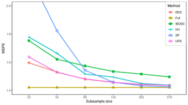
(a) Mean MSPE of Linear Regression

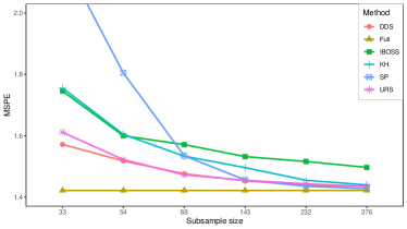
(b) Median MSPE of Linear Regression

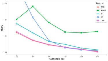
(c) Mean MSPE of Gaussion Process Regression

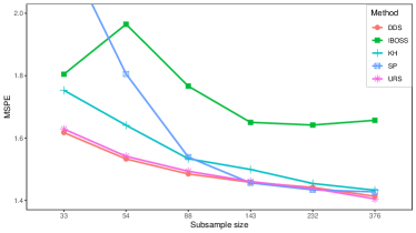
(d) Median MSPE of Gaussion Process Regression

Figure 6: The MSPE values of the fitted linear regression model and Gaussian process regression model established on different subsample strategies for the protein tertiary structure data.

In this subsection, we use the DDS for a real case study of the physicochemical properties of protein tertiary structure data set from the UCI machine learning repository (Dheeru and Taniskidou [4]). It contains $45730$ samples with 9 continuous attributes and 1 response variable.

First, we get rid of some outliers which results $45253$ samples and then rescale the data as the original data to use. Different from the simulation example of the borehole experiment, there is no guidance on the model for this real data. We consider the two models, linear regression model and Gaussian process regression model for the subdata by DDS, URS, IBOSS, KH and SP. The MSPE values of the $5$-fold cross-validation are calculated to compare the performance of different subsampling strategies. In the $5$-fold cross-validation, there are $5$ full data sets ${\mathcal{X}}_{\text{Full},1},\dots,{\mathcal{X}}_{\text{Full},5}$ and $5$ test data sets ${\mathcal{X}}_{\text{Test},1},\dots,{\mathcal{X}}_{\text{Test},5}$. For each ${\mathcal{X}}_{\text{Full},l}$, in the process of DDS, we use the first two dominated components which may explain more than $85\%$ of total variation in ${\mathcal{X}}_{\text{Full},l}$ by the principal component analysis. So the dimension of the rotated space is reduced to $2$. Here we select some numbers from the leave one out Fibonacci sequence as the subsample size $n$ for the good uniformity of the corresponding $2$-dimensional designs on $C^{2}$. The detail of the Fibonacci sequence can be seen in Fang et al. [6].

For each fitted model and subsample size $n$, the subsampling of URS, DDS and SP are repeated $100$ times but no repetition for deterministic subsampling method IBOSS and KH in each fold. Therefore, the mean, median and bounds of the MSPE results are determined by $500$, $500$, $500$, $5$ and $5$ values respectively for URS, DDS, SP, IBOSS and KH. Because of the simplicity of linear regression model, fitting such the model based on the full data is also considered. Figure 6 (a) and 6 (b) present the MSPE values of the fitted linear regression models for the subdata obtained by different subsampling methods. To present the results more explicitly, the vertical axises in Figure 6 are logarithmically transformed. The MSPE values of DDS are lower than that of URS from the versions of both mean and median. What’s more, the performance of DDS are better than IBOSS and KH. By Figure 8 (a) provided in Appendix B, the upper bound of the MSPE values of DDS are lower than that of IBOSS and KH for relatively large subsample size $n$. SP leads to lower MSPE values than DDS for $n\geq 232$, however the performance of SP is the worst while $n$ is relatively small, which is not robust for the subsample size.

For the Gaussian process regression model, training a model based on the full data in each fold is omitted because of its high complexity. For the subsampling methods, we set the same basis function, kernel function and hyper-parameter optimization method for each subdata obtained by each subsampling method. The corresponding MSPE values are shown in Figure 6 (c) and 6 (d). Compared to the result of the simple linear regression model, the performance of IBOSS in this high complexity model even become worse. URS, DDS and SP have similar performance when the subsample size $n$ is relatively large. However, DDS performs slightly better than URS when $n$ is relatively small while other methods are significantly worse than URS.

These results of the real case study confirm that, if there is no a priori knowledge about the true model, model-free subsampling methods are more appropriate. Moreover, DDS performs more robust than other model-free subsampling method for different model specificaiton and subsample sizes.

7 Conclusion

In this paper we provide a data-driven subsampling method that is model-free. This similarity of the subsamples with respect to the original data is measured by the generalized empirical $F$-discrepancy, which is asymptotic equivalent to the classical generalized ${\ell}_{2}$-discrepancy in the theory of uniform designs. The numerical examples show the effectiveness and robustness of the proposed DDS method, as well as its accelerated version (ADDS) in the high-dimensional cases. In addition, both DDS and ADDS have the capacity of parallel computation for the cases of decentralized data storage according to the use of sliced uniform designs.

Appendix A

Proof of Theorem 1. For simplicity, denote $\widetilde{{\mbox{\boldmath$x$}}}=T_{{\mathcal{X}}}({\mbox{\boldmath$x$}})$ for each ${\mbox{\boldmath$x$}}\in{\mathcal{X}}\cup{\mathcal{P}}$, and $\widetilde{{\mathcal{X}}}=T_{{\mathcal{X}}}({\mathcal{X}})$, $\widetilde{{\mathcal{P}}}=T_{{\mathcal{X}}}({\mathcal{P}})$, then $\widetilde{{\mathcal{X}}},\widetilde{{\mathcal{P}}}\subset C^{s}$, and the expression of $D^{2}({\mathcal{P}};{\mathcal{X}},{\mathbb{K}})$ in (5) can be rewritten as,

$$D^{2}({\mathcal{P}};{\mathcal{X}},{\mathbb{K}}) =\frac{1}{N^{2}}\sum_{i,k=1}^{N}{\mathbb{K}}(\widetilde{{\mbox{\boldmath$x$}}_{i}},\widetilde{{\mbox{\boldmath$x$}}_{k}})-\frac{2}{Nn}\sum_{i=1}^{N}\sum_{k=1}^{n}{\mathbb{K}}(\widetilde{{\mbox{\boldmath$x$}}_{i}},\widetilde{\bm{\xi}_{k}})+\frac{1}{n^{2}}\sum_{i,k=1}^{n}{\mathbb{K}}(\widetilde{\bm{\xi}_{i}},\widetilde{\bm{\xi}_{k}})$$

$$=\int_{C^{2s}}{\mathbb{K}}({\mbox{\boldmath$u$}},{\mbox{\boldmath$v$}})\mbox{d}F_{\widetilde{{\mathcal{X}}}}({\mbox{\boldmath$u$}})\mbox{d}F_{\widetilde{{\mathcal{X}}}}({\mbox{\boldmath$v$}})-\frac{2}{n}\sum_{k=1}^{n}\int_{C^{2s}}{\mathbb{K}}({\mbox{\boldmath$u$}},\widetilde{\bm{\xi}_{k}})\mbox{d}F_{\widetilde{{\mathcal{X}}}}({\mbox{\boldmath$u$}})+\frac{1}{n^{2}}\sum_{i,k=1}^{n}{\mathbb{K}}(\widetilde{\bm{\xi}_{i}},\widetilde{\bm{\xi}_{k}}),$$ (12)

where $F_{\widetilde{{\mathcal{X}}}}$ and $F_{\widetilde{{\mathcal{P}}}}$ are the ECDFs of $\widetilde{{\mathcal{X}}}$ and $\widetilde{{\mathcal{P}}}$, respectively. Because of the joint independence assumption for ${\mathcal{X}}$ in (6), $\widetilde{{\mathcal{X}}}$ also satisfies the joint independence as follows,

$$F_{\widetilde{{\mathcal{X}}}}({\mbox{\boldmath$u$}})=\prod_{j=1}^{s}F_{\widetilde{{\mathcal{X}}}_{(j)}}(u_{j}),~{}~{}~{}\forall~{}{\mbox{\boldmath$u$}}=(u_{1},\dots,u_{s})^{T}\in C^{s},$$

where $\widetilde{{\mathcal{X}}}_{(j)}=\{F_{{\mathcal{X}}_{(j)}}(x_{ij}),i=1,\dots,N\}$ is the set of values along the $j$th component of $\widetilde{{\mathcal{X}}}$, then by using the product form of ${\mathbb{K}}$, the integrations over $C^{2s}$ and $C^{s}$ in (12) could be derived into the product form as follows,

$$\int_{C^{2s}}{\mathbb{K}}({\mbox{\boldmath$u$}},{\mbox{\boldmath$v$}})\mbox{d}F_{\widetilde{{\mathcal{X}}}}({\mbox{\boldmath$u$}})\mbox{d}F_{\widetilde{{\mathcal{X}}}}({\mbox{\boldmath$v$}})= \prod_{j=1}^{s}\int_{0}^{1}\int_{0}^{1}K(u_{j},v_{j})\mbox{d}F_{\widetilde{{\mathcal{X}}}_{(j)}}(u_{j})\mbox{d}F_{\widetilde{{\mathcal{X}}}_{(j)}}(v_{j}),$$ (13)

$$\int_{C^{s}}{\mathbb{K}}({\mbox{\boldmath$u$}},\widetilde{\bm{\xi}_{k}})\mbox{d}F_{\widetilde{{\mathcal{X}}}}({\mbox{\boldmath$u$}})= \prod_{j=1}^{s}\int_{0}^{1}K(u_{j},F_{{\mathcal{X}}_{(j)}}(\xi_{kj}))\mbox{d}F_{\widetilde{{\mathcal{X}}}_{(j)}}(u_{j}).$$ (14)

For each $j=1,\dots,s$, there are also $N_{j}$ different values $\hat{x}_{1j}<\dots<\hat{x}_{N_{j}j}=1$ in ${\widetilde{{\mathcal{X}}}_{(j)}}$. Denote $\hat{x}_{0j}=0$, and the replication of $\hat{x}_{ij}$ by $n_{ij}$, then $\hat{x}_{ij}-\hat{x}_{i-1,j}=n_{ij}/N$, $i=1,\dots,N_{j}$. Based on the Mean Value Theorem, for any $v\in[0,1]$,

$$\int_{0}^{1}K(u,v)\mbox{d}u=\sum_{i=1}^{N_{j}}\int_{\hat{x}_{i-1,j}}^{\hat{x}_{ij}}K(u,v)\mbox{d}u=\sum_{i=1}^{N_{j}}K(u_{ij}^{*},v)\cdot\frac{n_{ij}}{N},$$

where $u_{ij}^{*}\in\left[\hat{x}_{i-1,j},\hat{x}_{ij}\right]$. Recall that the reproducing kernel $K$ satisfies the Lipschitz continuous with a constant $c_{2}$. It can be easily obtained that

$$\left|\int_{0}^{1}K(u,v)\mbox{d}F_{\widetilde{{\mathcal{X}}}_{(j)}}(u)-\int_{0}^{1}K(u,v)\mbox{d}u\right| =\left|\frac{1}{N}\sum_{i=1}^{N_{j}}n_{ij}\left(K(\hat{x}_{ij},v)-K(u_{ij}^{*},v)\right)\right|$$

$$\leq\frac{c_{2}}{N}\sum_{i=1}^{N_{j}}n_{ij}\left|\hat{x}_{ij}-u_{ij}^{*}\right|\leq\frac{c_{2}}{N^{2}}\sum_{i=1}^{N_{j}}n_{ij}^{2}.$$ (15)

Note that, the independent condition (6) also yields the following constraints about $N,N_{j}$ and $n_{ij}$, $N\geq\prod\limits_{l=1}^{s}N_{l}$ and $n_{ij}\leq c_{1}\prod\limits_{l\neq j}^{s}N_{l}$ for $i=1,\dots,N_{j},j=1,\dots,s,$ then the upper bound in (15) could be shrunk as follows,

$$\frac{c_{2}}{N^{2}}\sum_{i=1}^{N_{j}}n_{ij}^{2}\leq\frac{c_{2}}{\left(\prod_{l=1}^{s}N_{l}\right)^{2}}\sum_{i=1}^{N_{j}}\left[c_{1}^{2}\cdot\left(\frac{\prod_{l=1}^{s}N_{l}}{N_{j}}\right)^{2}\right]=\frac{c_{2}c_{1}^{2}}{N_{j}}={\mbox{\boldmath$O$}}(1/N_{j}),$$

which leads to

$$\int_{0}^{1}K(u,v)\mbox{d}F_{\widetilde{{\mathcal{X}}}_{(j)}}(u)=\int_{0}^{1}K(u,v)\mbox{d}u+{\mbox{\boldmath$O$}}(1/N_{j}).$$ (16)

Integrating (16) from 0 to 1 with the reference distribution $F_{\widetilde{{\mathcal{X}}}_{(j)}}$ yields

$$\int_{0}^{1}\int_{0}^{1}K(u,v)\mbox{d}F_{\widetilde{{\mathcal{X}}}_{(j)}}(u)\mbox{d}F_{\widetilde{{\mathcal{X}}}_{(j)}}(v) =\int_{0}^{1}\left[\int_{0}^{1}K(v,u)\mbox{d}F_{\widetilde{{\mathcal{X}}}_{(j)}}(v)\right]\mbox{d}u+{\mbox{\boldmath$O$}}(1/N_{j})$$

$$=\int_{0}^{1}\left[\int_{0}^{1}K(v,u)\mbox{d}v+{\mbox{\boldmath$O$}}(1/N_{j})\right]\mbox{d}u+{\mbox{\boldmath$O$}}(1/N_{j})$$

$$=\int_{0}^{1}\int_{0}^{1}K(u,v)\mbox{d}u\mbox{d}v+{\mbox{\boldmath$O$}}(1/N_{j}).$$ (17)

Substituting (17) into (13), and (16) into (14) obtains

$$\int_{C^{2s}}{\mathbb{K}}({\mbox{\boldmath$u$}},{\mbox{\boldmath$v$}})\mbox{d}F_{\widetilde{{\mathcal{X}}}}({\mbox{\boldmath$u$}})\mbox{d}F_{\widetilde{{\mathcal{X}}}}({\mbox{\boldmath$v$}}) =\prod_{j=1}^{s}\left[\int_{0}^{1}\int_{0}^{1}K(u,v)\mbox{d}u\mbox{d}v+{\mbox{\boldmath$O$}}(1/N_{j})\right]$$

$$=\int_{C^{2s}}{\mathbb{K}}({\mbox{\boldmath$u$}},{\mbox{\boldmath$v$}})\mbox{d}{\mbox{\boldmath$u$}}\mbox{d}{\mbox{\boldmath$v$}}+{\mbox{\boldmath$O$}}(1/N^{*}),$$ (18)

and

$$\int_{C^{s}}{\mathbb{K}}({\mbox{\boldmath$u$}},\widetilde{\bm{\xi}_{k}})\mbox{d}F_{\widetilde{{\mathcal{X}}}}({\mbox{\boldmath$u$}}) =\prod_{j=1}^{s}\left[\int_{0}^{1}K(u,F_{{\mathcal{X}}_{(j)}}(\xi_{kj}))\mbox{d}u+{\mbox{\boldmath$O$}}(1/N_{j})\right]$$

$$=\int_{C^{s}}{\mathbb{K}}({\mbox{\boldmath$u$}},\widetilde{\bm{\xi}_{k}})\mbox{d}{\mbox{\boldmath$u$}}+{\mbox{\boldmath$O$}}(1/N^{*}),$$ (19)

respectively. Finally, substituting (18) and (19) into (12) completes the proof.

To prove Lemma 1, we give the following lemma. Its proof can be referred to Lemma 3.3 in [8], and we omit it.

Lemma 2.

Define the kernel function on $C^{s}\times C^{s}$ with a product form ${\mathbb{K}}({\mbox{\boldmath$u$}},{\mbox{\boldmath$v$}})=\prod_{j=1}^{s}K(u_{j},y_{j}),$ where $K(u_{j},v_{j})$ is defined in (22). It follows that the components of ${\mathbb{K}}$ are

$${\mathbb{K}}_{\vartheta}({\mbox{\boldmath$u$}}_{\vartheta},{\mbox{\boldmath$v$}}_{\vartheta})=\left\{\begin{array}[]{ll}{\mathcal{L}}_{{\mathcal{S}}}({\mathbb{K}}({\mbox{\boldmath$u$}},{\mbox{\boldmath$v$}}))=1,&\quad\vartheta=\emptyset,\\ \prod_{j\in\vartheta}[K(u_{j},v_{j})-1],&\quad\vartheta\neq\emptyset,\end{array}\right.$$ (20)

where ${\mathcal{L}}_{j}$ denotes the operator ${\mathcal{L}}$ defined in (24) on the $j$th coordinate and ${\mathcal{L}}_{\vartheta}=\prod_{j\in\vartheta}{\mathcal{L}}_{j}$. Moreover, any $f\in\bm{X}_{p}(C^{s})$ has the following properties,

$$f_{\vartheta}({\mbox{\boldmath$v$}}_{\vartheta})=\beta^{-2|\vartheta|}\int_{C^{\vartheta}}\frac{\partial^{|\vartheta|}f_{\vartheta}}{\partial{\mbox{\boldmath$u$}}_{\vartheta}}\frac{\partial^{|\vartheta|}{\mathbb{K}}_{\vartheta}(\cdot,{\mbox{\boldmath$v$}}_{\vartheta})}{\partial{\mbox{\boldmath$u$}}_{\vartheta}}\text{d}{\mbox{\boldmath$u$}}_{\vartheta},$$

and $f({\mbox{\boldmath$v$}})=\langle f,{\mathbb{K}}(\cdot,{\mbox{\boldmath$v$}})\rangle.$ That indicates ${\mathbb{K}}$ is a reproducing kernel for $\bm{X}_{p}(C^{s})$.

Proof of Lemma 1: We give the details of the derivation from the two aspects of one-dimensional cases and multi-dimensional cases.

Define the Bernoulli polynomials $\{B_{n}(x)\}_{n=0}^{\infty}$ by the generating function $\frac{te^{xt}}{e^{t}-1}=\sum_{n=0}^{\infty}B_{n}(x)\frac{t^{n}}{n!}.$ The first few are $B_{0}(x)=1,B_{1}(x)=x-1/2,B_{3}(x)=x^{2}-x+1/6.$

(i) Consider the case of $\bm{s=1}$.
For any $p$, $1\leq p\leq\infty$, let

$$X_{p}\equiv\left\{f:\frac{\text{d}f}{\text{d}u}\in L_{p}([0,1])\right\}.$$ (21)

Suppose $K(\cdot,\cdot)$ have the following form

$$K(u,v)=M+\beta^{2}\left[\lambda(u)+\lambda(v)+\frac{1}{2}B_{2}\left(\bm{\{}u-v\bm{\}}\right)+B_{1}(u)B_{1}(v)\right],$$ (22)

where $\bm{\{}\cdot\bm{\}}$ denotes the fractional part of a real number, $\lambda$ is a function in the space $X_{\infty}$ satisfying $\int_{0}^{1}\lambda(x)\text{d}u=0$, $\beta$ is an arbitrary positive constant, and $M=1+\beta^{2}\int_{0}^{1}\left(\frac{\text{d}\lambda}{\text{d}u}\right)^{2}\text{d}u$. Then for any $v\in[0,1)$, the function $K(\cdot,v)\in X_{2}$, and for any function $f\in X_{2}$, the following results could be derived,

$$\frac{\partial K}{\partial u}=\beta^{2}\left[\frac{\text{d}\lambda}{\text{d}u}+B_{1}\left(\bm{\{}u-v\bm{\}}\right)+B_{0}(u)B_{1}(v)\right],$$ (23)

$$\beta^{-2}\int_{0}^{1}\frac{\partial K}{\partial u}\frac{\text{d}f}{\text{d}u}\text{d}u=f(v)-\int_{0}^{1}\left(f-\frac{\text{d}\lambda}{\text{d}u}\frac{\text{d}f}{\text{d}u}\right)\text{d}u.$$

Define a linear function of $f$ as follows

$${\mathcal{L}}(f)\equiv\int_{0}^{1}\left(f-\frac{\text{d}\lambda}{\text{d}u}\frac{\text{d}f}{\text{d}u}\right)\text{d}u.$$ (24)

Define an inner product and the induced norm as follows

$$\langle f,g\rangle={\mathcal{L}}(f){\mathcal{L}}(g)+\beta^{-2}\int_{0}^{1}\frac{\text{d}f}{\text{d}u}\frac{\text{d}g}{\text{d}u}\text{d}u,\qquad|||f|||_{p}=\left\|\left({\mathcal{L}}(f),\beta^{-1}\frac{\text{d}f}{\text{d}u}\right)\right\|_{p}.$$ (25)

Note that

$${\mathcal{L}}(K(\cdot,v))=\int_{0}^{1}\left(K-\frac{\text{d}\lambda}{\text{d}u}\frac{\partial K}{\partial u}\right)\text{d}u=M-\beta^{2}\int_{0}^{1}\left(\frac{\text{d}\lambda}{\text{d}u}\right)^{2}\text{d}u=1,$$ (26)

which leads to

$$\langle K(\cdot,v),f\rangle={\mathcal{L}}(f)+\beta^{-2}\int_{0}^{1}\frac{\partial K}{\partial u}\frac{\text{d}f}{\text{d}u}\text{d}u=f(v).$$

This result indicates $K$ defined in (22) is a reproducing kernel. For the linear function ${\mathcal{L}}$, by the Riesz Representation Theorem, there exists $\psi\in X_{2}$ such that ${\mathcal{L}}(f)=\langle\psi,f\rangle$ for any $f\in X_{2}$. As $K$ is a reproducing kernel, $\psi$ is the representer of ${\mathcal{L}}$, and from (26), we can obtain

$$\psi(v)=\langle K(\cdot,v),\psi\rangle={\mathcal{L}}(K(\cdot,v))=1,$$

which implys that the constant 1 is the representer for the linear functional ${\mathcal{L}}$, i.e.

$${\mathcal{L}}(f)=\langle 1,f\rangle,\quad\forall f\in X_{2}.$$ (27)

Denote

$${\mathcal{T}}(f)\equiv\frac{1}{N}\sum_{u\in{\mathcal{E}}}f(u)-\frac{1}{n}\sum_{\zeta\in{\mathcal{D}}}f(\zeta),$$ (28)

then ${\mathcal{T}}$ is also a bounded linear function. By the Riesz Representation Theorem, there exists $\phi\in X_{2}$ such that

$${\mathcal{T}}(f)=\langle\phi,f\rangle,~{}~{}~{}~{}\forall f\in X_{2}.$$ (29)

Note that $K$ is a reproducing kernel, then $\phi(v)=\langle K(\cdot,v),\phi\rangle$, based on (29), $\phi(v)$ is the results of the transformed $K(\cdot,v)$ under the linear function ${\mathcal{T}}$, i.e.

$$\phi(v)={\mathcal{T}}(K(\cdot,v))=\frac{1}{N}\sum_{u\in{\mathcal{E}}}K(u,v)-\frac{1}{n}\sum_{\zeta\in{\mathcal{D}}}K(\zeta,v).$$

From (27), (29) and (28), it can be easily obtained that ${\mathcal{L}}(\phi)=\langle 1,\phi\rangle={\mathcal{T}}(1)=0$, which leads to

$$|||\phi|||_{2}^{2}=\left\|\left({\mathcal{L}}(\phi),\beta^{-1}\frac{\text{d}\phi}{\text{d}v}\right)\right\|_{2}^{2}=\int_{0}^{1}\left(\beta^{-1}\frac{\text{d}\phi}{\text{d}v}\right)^{2}\text{d}v.$$ (30)

For any $f\in X_{p}$, define the generalized ${\ell}_{p}$-variation as

$$V_{p}(f)\equiv|||f-{\mathcal{L}}(f)|||_{p}=\left\|\beta^{-1}\frac{\text{d}f}{\text{d}v}\right\|_{p},$$ (31)

then we could obtain the following inequality by the H$\ddot{\text{o}}$lder inequality,

$$|{\mathcal{T}}(f)|=|\langle\phi,f\rangle|=\beta^{-2}\left|\int_{0}^{1}\frac{\text{d}\phi}{\text{d}v}\frac{\text{d}f}{\text{d}v}\text{d}v\right|\leq|||\phi|||_{2}V_{2}(f).$$ (32)

On the basis of the partial derivative of $K$ in (23), we have

$$\frac{\text{d}\phi}{\text{d}v}=\frac{\beta^{2}}{N}\sum_{u\in{\mathcal{E}}}\left[B_{1}\left(\bm{\{}v-u\bm{\}}\right)+B_{1}(u)\right]-\frac{\beta^{2}}{n}\sum_{\zeta\in{\mathcal{D}}}\left[B_{1}\left(\bm{\{}v-\zeta\bm{\}}\right)+B_{1}(\zeta)\right].$$ (33)

Note that for any $u,\zeta\in[0,1]$, according to the properties of $B_{n}$,

$$\int_{0}^{1}\left[B_{1}\left(\bm{\{}v-u\bm{\}}\right)+B_{1}(u)\right]\left[B_{1}\left(\bm{\{}v-\zeta\bm{\}}\right)+B_{1}(\zeta)\right]\text{d}v=\frac{1}{2}B_{2}\left(\bm{\{}u-\zeta\bm{\}}\right)+B_{1}(u)B_{1}(\zeta),$$ (34)

then substituting (33) into (30) and using the integral result in (34), we can compute the squared norm of $\phi$ as follows

$$|||\phi|||_{2}^{2} =\frac{\beta^{2}}{N^{2}}\sum_{u,\check{u}\in{\mathcal{E}}}\left[\frac{1}{2}B_{2}\left(\bm{\{}u-\check{u}\bm{\}}\right)+B_{1}(u)B_{1}(\check{u})\right]-\frac{2\beta^{2}}{Nn}\sum_{u\in{\mathcal{E}},\zeta\in{\mathcal{D}}}\left[\frac{1}{2}B_{2}\left(\bm{\{}u-\zeta\bm{\}}\right)+B_{1}(u)B_{1}(\zeta)\right]$$

$$\quad+\frac{\beta^{2}}{n^{2}}\sum_{\zeta,\check{\zeta}\in{\mathcal{D}}}\left[\frac{1}{2}B_{2}\left(\bm{\{}\zeta-\check{\zeta}\bm{\}}\right)+B_{1}(\zeta)B_{1}(\check{\zeta})\right]$$

$$=\frac{1}{N^{2}}\sum_{u,\check{u}\in{\mathcal{E}}}K(u,\check{u})-\frac{2}{Nn}\sum_{u\in{\mathcal{E}},\zeta\in{\mathcal{D}}}K(u,\zeta)+\frac{1}{n^{2}}\sum_{\zeta,\check{\zeta}\in{\mathcal{D}}}K(\zeta,\check{\zeta})=D_{K}^{2}({\mathcal{E}},{\mathcal{D}}).$$

Replacing $|||\phi|||_{2}$ in (32) with $D_{K}({\mathcal{E}},{\mathcal{P}})$, we achieve the inequality in Lemma 1 for $s=1$.

(ii) Consider the case of $\bm{s\geq 2}$.
Let ${\mathcal{S}}=\{1,\dots,s\}$ be the set of coordinate indices. For any $\vartheta\subseteq{\mathcal{S}}$, let $|\vartheta|$ denote its cardinality and $C^{\vartheta}=[0,1]^{\vartheta}$ the $|\vartheta|$-dimensional unit cube involving the coordinates in $\vartheta$, ${\mbox{\boldmath$u$}}_{\vartheta}$ the vector containing the components of $u$ whose indices are in $\vartheta$, and $\mathrm{d}{\mbox{\boldmath$u$}}_{\vartheta}=\prod_{j\in\vartheta}\mathrm{d}u_{j}$ the uniform measure on $C^{\vartheta}$. The multidimensional generalization of $X_{p}$, the space of integrands defined in (21), is a space of functions whose mixed partial derivatives are all integrable,

$${\mbox{\boldmath$X$}}_{p}\equiv{\mbox{\boldmath$X$}}_{p}(C^{s})\equiv\left\{f:\frac{\partial^{|\vartheta|}f}{\partial{\mbox{\boldmath$u$}}_{\vartheta}}\in L_{p}(C^{\vartheta}),~{}\forall\vartheta\subseteq{\mathcal{S}}\right\}.$$

Let ${\mathcal{L}}_{j}$ denote the operator ${\mathcal{L}}$ defined in (24) on the $j$th coordinate, ${\mathcal{L}}_{\vartheta}=\prod_{j\in\vartheta}{\mathcal{L}}_{j}$, and ${\mathcal{L}}_{\emptyset}$ be defined as the identity. For any $f\in{\mbox{\boldmath$X$}}_{p}(C^{s})$, iteratively define its components $f_{\vartheta}={\mathcal{L}}_{{\mathcal{S}}-\vartheta}f-\sum_{\omega\subset\vartheta}f_{\omega},\forall\vartheta\subseteq{\mathcal{S}}.$ These components possess the following properties:

$${\mathcal{L}}_{j}(f_{\vartheta})=\left\{\begin{array}[]{ll}0,&~{}j\in\vartheta,\\ f_{\vartheta},&~{}j\notin\vartheta,\end{array}\right.\quad\text{and}\quad f=\sum_{\vartheta\subseteq{\mathcal{S}}}f_{\vartheta}.$$

Then define the inner product $\langle\cdot,\cdot\rangle$ on ${\mbox{\boldmath$X$}}_{2}(C^{s})$ and the norm $|||\cdot|||_{p}$ on ${\mbox{\boldmath$X$}}_{p}(C^{s})$ as the generalizations of those in (25) as follows,

$$\langle f,g\rangle=\sum_{\vartheta\subseteq{\mathcal{S}}}\beta^{-2|\vartheta|}\int_{C^{\vartheta}}\frac{\partial^{|\vartheta|}f_{\vartheta}}{\partial{\mbox{\boldmath$u$}}_{\vartheta}}\frac{\partial^{|\vartheta|}g_{\vartheta}}{\partial{\mbox{\boldmath$u$}}_{\vartheta}}\text{d}{\mbox{\boldmath$u$}}_{\vartheta},\qquad|||f|||_{p}=\left\|\left(\beta^{-|\vartheta|}\frac{\partial^{|\vartheta|}f_{\vartheta}}{\partial{\mbox{\boldmath$u$}}_{\vartheta}}\right)_{\vartheta\subseteq{\mathcal{S}}}\right\|_{p}.$$

Define the kernel function on $C^{s}\times C^{s}$ with a product form ${\mathbb{K}}({\mbox{\boldmath$u$}},{\mbox{\boldmath$v$}})=\prod_{j=1}^{s}K(u_{j},v_{j}),$ where $K(u_{j},v_{j})$ is defined in (22). Then ${\mathbb{K}}$ is the reproducing kernel for ${\mbox{\boldmath$X$}}_{p}(C^{s})$ indicated from Lemma 2.

Now define the linear function ${\mathcal{T}}$ with the same form as the case of $s=1$ in (28), then its representer $\phi$ satisfies ${\mathcal{T}}({\mathbb{K}}(\cdot,{\mbox{\boldmath$v$}}))=\langle\phi,{\mathbb{K}}(\cdot,{\mbox{\boldmath$v$}})\rangle$. Note that ${\mathbb{K}}$ is a reproducing kernel, and $\phi({\mbox{\boldmath$v$}})=\langle{\mathbb{K}}(\cdot,{\mbox{\boldmath$v$}}),\phi\rangle$, so $\phi({\mbox{\boldmath$v$}})$ could be presented as the following linear combination of the values of ${\mathbb{K}}(\cdot,{\mbox{\boldmath$v$}})$ upon the two sets ${\mathcal{E}}$ and ${\mathcal{D}}$,

$$\phi({\mbox{\boldmath$v$}})={\mathcal{T}}({\mathbb{K}}(\cdot,{\mbox{\boldmath$v$}}))=\frac{1}{N}\sum_{{\mbox{\boldmath$u$}}\in{\mathcal{E}}}{\mathbb{K}}({\mbox{\boldmath$u$}},{\mbox{\boldmath$v$}})-\frac{1}{n}\sum_{\bm{\zeta}\in{\mathcal{D}}}{\mathbb{K}}(\bm{\zeta},{\mbox{\boldmath$v$}}),$$

then its components are $\phi_{\vartheta}({\mbox{\boldmath$v$}}_{\vartheta})=\frac{1}{N}\sum_{{\mbox{\boldmath$u$}}\in{\mathcal{E}}}\prod_{j\in\vartheta}\left[K(u_{j},v_{j})-1\right]-\frac{1}{n}\sum_{\bm{\zeta}\in{\mathcal{D}}}\prod_{j\in\vartheta}\left[K(\zeta_{j},v_{j})-1\right]$ by using the expression of ${\mathbb{K}}$’s components in (20). On the basis of the partial derivative of $K$ in (23), the partial derivative of $\phi$ could be computed as

$$\frac{\partial^{|\vartheta|}\phi_{\vartheta}}{\partial{\mbox{\boldmath$v$}}_{\vartheta}} =\frac{\beta^{2|\vartheta|}}{N}\sum_{{\mbox{\boldmath$u$}}\in{\mathcal{E}}}\prod_{j\in\vartheta}\left[\lambda^{\prime}(v_{j})+B_{1}\left(\bm{\{}v_{j}-u_{j}\bm{\}}\right)+B_{1}(u_{j})\right]$$

$$\quad-\frac{\beta^{2|\vartheta|}}{n}\sum_{\bm{\zeta}\in{\mathcal{D}}}\prod_{j\in\vartheta}\left[\lambda^{\prime}(v_{j})+B_{1}\left(\bm{\{}v_{j}-\zeta_{j}\bm{\}}\right)+B_{1}(\zeta_{j})\right],$$

where $\lambda^{\prime}$ is the derivative of $\lambda$. For any $u,\zeta\in[0,1]$, according to the properties of $B_{n}$, the constraint of $M$ and the form of $K$ in (22), we have

$$\int_{0}^{1}\left[\lambda^{\prime}(v)+B_{1}\left(\bm{\{}v-u\bm{\}}\right)+B_{1}(u)\right]\left[\lambda^{\prime}(v)+B_{1}\left(\bm{\{}v-\zeta\bm{\}}\right)+B_{1}(\zeta)\right]\text{d}v$$

$$=\int_{0}^{1}\left(\lambda^{\prime}(v)\right)^{2}\text{d}v+\lambda(u)+\lambda(\zeta)+\frac{1}{2}B_{2}\left(\bm{\{}u-\zeta\bm{\}}\right)+B_{1}(u)B_{1}(\zeta)$$

$$=\beta^{-2}(M-1)+\lambda(u)+\lambda(\zeta)+\frac{1}{2}B_{2}\left(\bm{\{}u-\zeta\bm{\}}\right)+B_{1}(u)B_{1}(\zeta)$$

$$=\beta^{-2}\left(K(u,\zeta)-1\right).$$

Combining this result with the formula of the components of ${\mathbb{K}}$ presented in Lemma 2, we have

$$\int_{C^{\vartheta}}\left(\frac{\partial^{|\vartheta|}\phi_{\vartheta}}{\partial{\mbox{\boldmath$v$}}_{\vartheta}}\right)^{2}\text{d}{\mbox{\boldmath$v$}}_{\vartheta} =\frac{\beta^{2|\vartheta|}}{N^{2}}\sum_{{\mbox{\boldmath$u$}},\check{{\mbox{\boldmath$u$}}}\in{\mathcal{E}}}\prod_{j\in\vartheta}\left[K(u_{j},\check{u}_{j})-1\right]-\frac{2\beta^{2|\vartheta|}}{Nn}\sum_{{\mbox{\boldmath$u$}}\in{\mathcal{E}},\bm{\zeta}\in{\mathcal{D}}}\prod_{j\in\vartheta}\left[K(u_{j},\zeta_{j})-1\right]$$

$$\quad+\frac{\beta^{2|\vartheta|}}{n^{2}}\sum_{\bm{\zeta},\check{\bm{\zeta}}\in{\mathcal{D}}}\prod_{j\in\vartheta}\left[K(\zeta_{j},\check{\zeta}_{j})-1\right]$$

$$=\frac{\beta^{2|\vartheta|}}{N^{2}}\sum_{{\mbox{\boldmath$u$}},\check{{\mbox{\boldmath$u$}}}\in{\mathcal{E}}}{\mathbb{K}}_{\vartheta}({\mbox{\boldmath$u$}}_{\vartheta},\check{{\mbox{\boldmath$u$}}}_{\vartheta})-\frac{2\beta^{2|\vartheta|}}{Nn}\sum_{{\mbox{\boldmath$u$}}\in{\mathcal{E}},\bm{\zeta}\in{\mathcal{D}}}{\mathbb{K}}_{\vartheta}({\mbox{\boldmath$u$}}_{\vartheta},\check{\bm{\zeta}}_{\vartheta})+\frac{\beta^{2|\vartheta|}}{n^{2}}\sum_{\bm{\zeta},\check{\bm{\zeta}}\in{\mathcal{D}}}{\mathbb{K}}_{\vartheta}(\bm{\zeta}_{\vartheta},\check{\bm{\zeta}}_{\vartheta}).$$

For any $f\in{\mbox{\boldmath$X$}}_{p}(C^{s})$, let $V_{p,\vartheta}\equiv\left\|\frac{\partial^{|\vartheta|}f_{\vartheta}}{\partial{\mbox{\boldmath$v$}}_{\vartheta}}\right\|_{p}$ and define the generalized ${\ell}_{p}$-variation as

$$V_{p}(f)\equiv|||f-{\mathcal{L}}_{{\mathcal{S}}}(f)|||_{p}=\left\|\left(\beta^{-|\vartheta|}V_{p,\vartheta}(f)\right)_{\vartheta\neq\emptyset}\right\|_{p}=\left\|\left(\beta^{-|\vartheta|}\frac{\partial^{|\vartheta|}f_{\vartheta}}{\partial{\mbox{\boldmath$v$}}_{\vartheta}}\right)_{\vartheta\neq\emptyset}\right\|_{p}.$$ (35)

Recall that ${\mathbb{K}}$ is the reproducing kernel, combined with the Riesz Representation Theorem, it can be inferred that ${\mathcal{L}}_{S}(\phi)=0$, and

$$|{\mathcal{T}}(f)| =|\langle\phi,f\rangle|=\left|\sum_{\vartheta\neq\emptyset}\beta^{-2|\vartheta|}\int_{C^{\vartheta}}\frac{\partial^{|\vartheta|}\phi_{\vartheta}}{\partial{\mbox{\boldmath$v$}}_{\vartheta}}\frac{\partial^{|\vartheta|}f_{\vartheta}}{\partial{\mbox{\boldmath$v$}}_{\vartheta}}\text{d}{\mbox{\boldmath$v$}}_{\vartheta}\right|$$

$$\leq\sum_{\vartheta\neq\emptyset}\beta^{-2|\vartheta|}\int_{C^{\vartheta}}\left|\frac{\partial^{|\vartheta|}\phi_{\vartheta}}{\partial{\mbox{\boldmath$v$}}_{\vartheta}}\frac{\partial^{|\vartheta|}f_{\vartheta}}{\partial{\mbox{\boldmath$v$}}_{\vartheta}}\right|\text{d}{\mbox{\boldmath$v$}}_{\vartheta}\leq\sum_{\vartheta\neq\emptyset}\left\|\beta^{-|\vartheta|}\frac{\partial^{|\vartheta|}\phi_{\vartheta}}{\partial{\mbox{\boldmath$v$}}_{\vartheta}}\right\|_{2}\left\|\beta^{-|\vartheta|}\frac{\partial^{|\vartheta|}f_{\vartheta}}{\partial{\mbox{\boldmath$v$}}_{\vartheta}}\right\|_{2}\leq|||\phi|||_{2}V_{2}(f),$$ (36)

by H$\ddot{\text{o}}$lder inequality and Cauchy–Schwarz inequality, where

$$|||\phi|||_{2}^{2} =\left\|\left(\beta^{-|\vartheta|}\frac{\partial^{|\vartheta|}\phi_{\vartheta}}{\partial{\mbox{\boldmath$v$}}_{\vartheta}}\right)_{\vartheta\subseteq{\mathcal{S}}}\right\|_{2}^{2}=\sum_{\vartheta\subseteq{\mathcal{S}}}\left\|\beta^{-|\vartheta|}\frac{\partial^{|\vartheta|}\phi_{\vartheta}}{\partial{\mbox{\boldmath$v$}}_{\vartheta}}\right\|_{2}^{2}=\sum_{\vartheta\subseteq{\mathcal{S}}}\int_{C^{\vartheta}}\left(\beta^{-|\vartheta|}\frac{\partial^{|\vartheta|}\phi_{\vartheta}}{\partial{\mbox{\boldmath$v$}}_{\vartheta}}\right)^{2}\text{d}{\mbox{\boldmath$v$}}_{\vartheta}$$

$$=\frac{1}{N^{2}}\sum_{{\mbox{\boldmath$u$}},\check{{\mbox{\boldmath$u$}}}\in{\mathcal{E}}}\sum_{\vartheta\subseteq{\mathcal{S}}}{\mathbb{K}}_{\vartheta}({\mbox{\boldmath$u$}}_{\vartheta},\check{{\mbox{\boldmath$u$}}}_{\vartheta})-\frac{2}{Nn}\sum_{{\mbox{\boldmath$u$}}\in{\mathcal{E}},\bm{\zeta}\in{\mathcal{D}}}\sum_{\vartheta\subseteq{\mathcal{S}}}{\mathbb{K}}_{\vartheta}({\mbox{\boldmath$u$}}_{\vartheta},\bm{\zeta}_{\vartheta})+\frac{1}{n^{2}}\sum_{\bm{\zeta},\check{\bm{\zeta}}\in{\mathcal{D}}}\sum_{\vartheta\subseteq{\mathcal{S}}}{\mathbb{K}}_{\vartheta}(\bm{\zeta}_{\vartheta},\check{\bm{\zeta}}_{\vartheta})$$

$$=\frac{1}{N^{2}}\sum_{{\mbox{\boldmath$u$}},\check{{\mbox{\boldmath$u$}}}\in{\mathcal{E}}}{\mathbb{K}}({\mbox{\boldmath$u$}},\check{{\mbox{\boldmath$u$}}})-\frac{2}{Nn}\sum_{{\mbox{\boldmath$u$}}\in{\mathcal{E}},\bm{\zeta}\in{\mathcal{D}}}{\mathbb{K}}({\mbox{\boldmath$u$}},\bm{\zeta})+\frac{1}{n^{2}}\sum_{\bm{\zeta},\check{\bm{\zeta}}\in{\mathcal{D}}}{\mathbb{K}}(\bm{\zeta},\check{\bm{\zeta}})=D_{{\mathbb{K}}}^{2}({\mathcal{E}},{\mathcal{D}}).$$

Note that, the definition of the generalized ${\ell}_{p}$-variation $V_{p}(f)$ both in (31) for $s=1$ and in (35) for $s\geq 2$ are relative to $\beta$, a term in the kernel function $K$, therefore $V_{p}(f)$ could be denoted by $V_{p}(f,K)$ for $s=1$ and $V_{p}(f,{\mathbb{K}})$ for $s>1$. Replace $|||\phi|||_{2}$ in (36) with $D_{{\mathbb{K}}}({\mathcal{E}},{\mathcal{P}})$ and we complete the proof.

Appendix B

The MSPE values of numerical examples are given in Tables 2, 3, 4 and 5. For the deterministic method IBOSS and KH, the MSPE values for each subsample size $n$ are given. For URS, DDS and SP, the mean, median, upper bound and low bound of MSPE for each subsample size $n$ are given for these methods are executed multiple replications. Figures 7, 8 are provide to compare the upper and lower bound of MSPE for different methods in each numerical example.

Table 2: The MSPE values of different methods applied to the real life borehole example while working model is misspecified as the linear regression model. The MSPE value of prediction based on full data is 34.19551.

Method	n=50	n=80	n=150	n=250	n=400
URS_Mean	43.54	39.52	36.97	35.86	35.20
URS_Median	41.43	38.73	36.51	35.60	35.05
URS_Upper	58.01	45.84	40.42	37.77	36.40
URS_Lower	36.68	35.68	35.00	34.70	34.52
DDS_Mean	38.37	35.43	34.83	34.51	34.48
DDS_Median	37.50	35.19	34.74	34.55	34.45
DDS_Upper	45.74	36.90	35.66	34.79	34.77
DDS_Lower	35.51	34.53	34.36	34.30	34.29
SP_Mean	34.31	34.26	34.23	34.22	34.22
SP_Median	34.31	34.26	34.23	34.22	34.21
SP_Upper	34.41	34.32	34.26	34.24	34.23
SP_Lower	34.24	34.22	34.21	34.21	34.21
IBOSS	55.73	47.33	44.02	42.83	41.58
KH	38.89	39.11	36.27	38.64	35.22

Table 3: The MSPE values $\left(\times 10^{-2}\right)$ of different methods applied to the real life borehole example while working model is misspecified as the generlized linear regression model. The MSPE value of prediction based on full data is $5.312\times 10^{-2}$.

Method	n=50	n=80	n=150	n=250	n=400
URS_Mean	7.900	6.872	6.091	5.771	5.598
URS_Media	7.463	6.662	6.001	5.721	5.562
URS_Upper	10.861	8.437	6.860	6.209	5.891
URS_Lower	6.125	5.815	5.595	5.477	5.420
DDS_Mean	6.505	6.001	5.630	5.504	5.426
DDS_Median	6.349	5.903	5.597	5.482	5.410
DDS_Upper	7.831	6.781	5.884	5.595	5.560
DDS_Lower	5.746	5.495	5.439	5.387	5.354
SP_Mean	5.787	5.812	6.033	6.460	6.576
SP_Median	5.553	5.466	5.469	5.648	5.822
SP_Upper	6.096	6.554	7.823	9.818	9.935
SP_Lower	5.399	5.362	5.342	5.346	5.368
IBOSS	8.873	8.116	7.367	7.070	6.672
KH	251.026	11.146	12.186	6.604	11.085

Table 4: The MSPE values of different methods applied to the real case example while model is specified as the linear regression model. The MSPE value of prediction based on full data is 26.34.

Method	n=33	n=54	n=88	n=143	n=232	n=376
URS_Mean	43.36	33.73	30.25	28.69	27.71	27.20
URS_Media	40.82	33.26	29.67	28.47	27.74	27.18
URS_Upper	60.46	40.62	34.40	31.16	29.01	28.11
URS_Lower	31.69	28.88	27.82	27.08	26.68	26.47
DDS_Mean	39.46	33.85	30.16	28.60	27.59	27.22
DDS_Median	37.28	32.93	29.90	28.36	27.46	27.19
DDS_Upper	53.18	40.69	33.99	30.96	28.74	28.18
DDS_Lower	30.64	28.63	27.68	27.13	26.66	26.45
SP_Mean	166.75	66.58	34.88	28.68	27.06	26.57
SP_Median	151.97	63.78	34.22	28.56	27.23	26.73
SP_Upper	251.84	99.13	41.47	30.65	27.93	27.06
SP_Lower	95.41	42.22	29.49	27.11	26.28	26.04
IBOSS	56.66	41.77	37.50	34.20	32.79	31.33
KH	60.14	46.05	32.78	31.23	28.10	27.33

Table 5: The MSPE values of different methods applied to the real case example while model is specified as the Gaussian process regression model.

Method	n=33	n=54	n=88	n=143	n=232	n=376
URS_Mean	45.23	35.60	31.47	29.20	27.47	25.52
URS_Media	42.54	34.79	31.16	28.89	27.44	25.41
URS_Upper	68.25	45.88	36.98	32.35	29.45	27.39
URS_Lower	32.51	29.35	27.67	27.01	25.74	24.01
DDS_Mean	44.01	35.17	31.10	29.01	27.67	25.91
DDS_Median	41.44	34.11	30.54	28.71	27.66	25.90
DDS_Upper	62.42	44.93	36.71	31.92	29.39	27.67
DDS_Lower	31.54	29.36	27.98	27.05	26.04	24.32
SP_Mean	170.16	67.62	35.14	28.80	27.15	26.51
SP_Median	163.25	63.88	34.59	28.60	27.17	26.75
SP_Upper	265.56	102.58	42.13	30.69	27.95	26.98
SP_Lower	96.22	42.55	29.63	27.26	26.21	25.53
IBOSS	63.76	92.23	58.39	44.70	43.82	45.39
KH	56.64	43.75	34.18	31.58	28.47	27.09

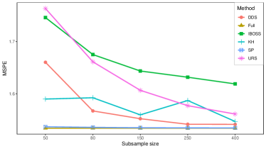
(a) The Upper Bound of MSPE of Linear Regression upon the Original Data

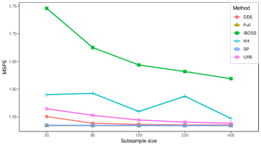
(b) The Lower Bound MSPE of Linear Regression upon the Original Data

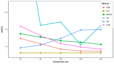
(c) The Upper Bound of MSPE of Generalized Linear Regression upon the Transformed Data

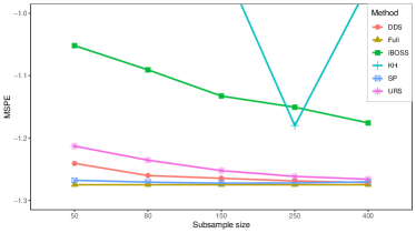
(d) The Lower Bound of MSPE of Generalized Linear Regression upon the Transformed Data

Figure 7: The bound of MSPE values of the fitted linear regression model based on the subdata sets obtained through different subsample strategies from the full data sets with the original form and the transformed form for the borehole experiments.

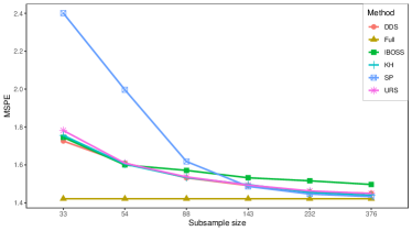
(a) The Upper Bound of MSPE of Linear Regression

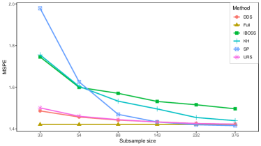
(b) The Lower Bound of MSPE of Linear Regression

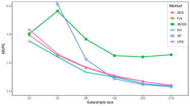
(c) The Upper Bound of MSPE of Gaussion Process Regression

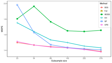
(d) The Lower Bound of MSPE of Gaussion Process Regression

Figure 8: The bound of MSPE values of the fitted linear regression model and Gaussian process regression model established on different subsample strategies for the protein tertiary structure data.

References

[1] Bottou, L., Curtis, F. E. and Nocedal, J. (2018), Optimization methods for large-scale machine learning, SIAM Review60(2), 223–311.
[2] Chen, Y., Welling, M. and Smola, A.(2012),
Chen, Yutian and Welling, Max and Smola, Alex,
Proceedings of the Twenty-Sixth Conference on Uncertainty in Artificial Intelligence.
[3] Chen, H., Huang, H. Z., Lin, D. K. J. and Liu, M. Q. (2016),
Uniform sliced Latin hypercube designs,
Applied Stochastic Models in Business and Industry32(5), 574–584.
[4] Dheeru, D. and Karra Taniskidou, E. (2017),
UCI Machine Learning Repository,
URL: http://archive.ics.uci.edu/ml.
[5] Fang, K. T., Li, R. and Sudjianto, A. (2006),
Design and Modeling for Computer Experiments,
Chapman and Hall/CRC, London.
[6]
Fang, K. T., Liu, M. Q., Qin, H. and Zhou, Y. D. (2018),
Theory and Application of Uniform Experimental designs,
Springer & Science Press, Singapore & Beijing.
[7] Fang, K. T. and Wang, Y. (1994),
Number-theoretic Methods in Statistics,
Chapman and Hall, London.
[8] Hickernell, F. J. (1998a),
A generalized discrepancy and quadrature error bound,
Mathematics of computation67(221), 299–322.
[9] Hickernell, F. J. (1998b), Lattice rules: how well do they measure up? In: P. Hellekalek and G. Larcher, Eds., Random and Quasi-Random Point Sets, Lecture Notes in Statistics, vol. 138. Springer, New York, 109–166.
[10] Ho, W. M. and Xu, Z. Q. (2000),
Applications of uniform design to computer experiments,
Journal of Chinese Statistical Association38, 395–410.
[11] Mahoney, M. W. (2011),
Randomized algorithms for matrices and data,
Foundations and Trendin Machine Learning3(2), 123–224.
[12] Mak, S. and Joseph V. R. (2018),
Support points,
Annals of Statistics, 46(6A), 2562–2592.
[13]
Morris, M. D., Mitchell, T. J. and Ylvisaker, D. (1993),
Bayesian design and analysis of computer experiments:
use of derivatives in surface prediction,
Technometrics, 35(3), 243–255.
[14] Niederreiter, H. (1992),
Random Number Generation and Quasi-Monte Carlo Methods,
SIAM CBMS-NSF Regional Conference Series in
Applied Mathematics, Philadephia.
[15] Wang, H. Y., Zhu, R. and Ma, P. (2018),
Optimal Subsampling for Large Sample Logistic Regression,
Journal of the American Statistical Association,
113(522), 829–844.
[16] Wang, H. Y., Yang, M. and Stufken, J. (2019),
Information-Based Optimal Subdata Selection for Big Data
Linear Regression,
Journal of the Amarican Statistical Association114(525), 393–405.
[17] Weyl, H. (1916), ber die gleichverteilung der zahlem mod eins,
Mathematische Annalen, 77(3), 313–352.
[18] Woodruff, D. P. (2014),
Sketching as a tool for numerical linear algebra,
Foundations and Trendin Theoretical Computer Science, 10(1–2): 1–157.
[19]
Worley, B. A. (1987),
Deterministic uncertainty analysis (No. CONF-871101-30),
Oak Ridge National Lab., TN (USA).
[20] Xu, J., He, X., Duan, X. Y. and Wang, Z. M. (2018),
Sliced Latin Hypercube Designs for Computer
Experiments With Unequal Batch Sizes, IEEE access, 6, 60396-60402.
[21] Yuan, R., Guo, B. and Liu, M. Q. (2019),
Flexible sliced Latin hypercube designs with slices of different sizes.
Statistical Papers, online.
[22]
Zhang, A. J., Li, H. Y., Quan, S. J., and Yang, Z. B. (2018),
UniDOE: Uniform Design of Experiments,
R package version 1.0.2.
[23] Zhou, Y. D., Fang, K. T. and Ning, J. H. (2013), Mixture discrepancy for quasi-random point sets, Journal of Complexity, 29(3–4), 283–301.