A penalized criterion for selecting the number of clusters for K-medians

Abstract

Clustering is a usual unsupervised machine learning technique for grouping the data points into groups based upon similar features. We focus here on unsupervised clustering for contaminated data, i.e in the case where K-medians algorithm should be preferred to K-means because of its robustness. More precisely, we concentrate on a common question in clustering: how to chose the number of clusters? The answer proposed here is to consider the choice of the optimal number of clusters as the minimization of a penalized criterion. In this paper, we obtain a suitable penalty shape for our criterion and derive an associated oracle-type inequality. Finally, the performance of this approach with different types of K-medians algorithms is compared on a simulation study with other popular techniques. All studied algorithms are available in the R package Kmedians on CRAN.

Keywords: Clustering, K-medians, Robust statistics

1 Introduction

Clustering is unsupervised machine learning technique which is defined as the algorithm for grouping the data points into a collection of groups based upon similar features. Clustering is generally used for data compression in image processing, which is also known as vector quantization (Gersho and Gray,, 2012). There is a vast literature on clustering techniques and general references regarding clustering may be found in Spath, (1980); Jain and Dubes, (1988); Mirkin, (1996); Jain et al., (1999); Berkhin, (2006); Kaufman and Rousseeuw, (2009). Classification methods can be categorized as hard clustering (K-means, K-medians and hierarchical clustering) and soft clustering (Fuzzy K-means (Dunn,, 1973; Bezdek,, 2013) and Mixture Models). In Hard clustering methods, each data point belongs to only one group, while for soft ones, a probability or likelihood of a data point to be in the cluster is assigned. Then, each data point can be a member of more than one group.

We focus here on hard clustering methods. The most popular partitioning clustering methods are the non sequential (Forgy,, 1965) and the sequential (MacQueen,, 1967) versions of the K-means algorithms. The aim of the K-means algorithm is to minimize the sum of squared distances between the data points and their respective cluster centroid. More precisely, considering $X_{1},...,X_{n}$ be random vectors taking values in $\mathbb{R}^{d}$, the aim is to find k centroids $\left\{c_{1},...,c_{k}\right\}$ minimizing the empirical distortion

$$\frac{1}{n}\sum_{i=1}^{n}\min_{j=1,..,k}\left\|X_{i}-c_{j}\right\|^{2}.$$ (1)

Nevertheless, in many real-world applications, collected data are contaminated by noise with heavy-tailed distribution and might contain outliers of large magnitude and K-means methods are very sensitive to the presence of these outliers. It is then necessary to apply methods which produce reliable robust outcomes. The K-medians clustering is proposed to get more robust clustering algorithms; it was suggested by MacQueen, (1967) and developed by Kaufman and Rousseeuw, (2009). K-medians clustering is a variant of K-means clustering where instead of calculating the mean of each cluster to determine its centroid, we calculate instead the geometric median. It consists in considering criteria based on least norms instead of least squared norms. More precisely, considering the same sequence of i.i.d copies $X_{1},...,X_{n}$, the objective of K-medians clustering is to minimize the empirical $L^{1}$-distortion :

$$\frac{1}{n}\sum_{i=1}^{n}\min_{j=1,..,k}\left\|X_{i}-c_{j}\right\|.$$

In practical applications, the number of clusters k is unknown. In this paper, we will focus on the choice of optimal number of clusters for robust clustering. Several methods for determining the optimal number of clusters have been studied for K-means algorithms and can be easily adapted for K-medians. In practice, one of the most used method for determining the optimal number of clusters is elbow method. Other methods often used are the Silhouette (Kaufman and Rousseeuw,, 2009) and the Gap Statistic (Tibshirani et al.,, 2001). The silhouette coefficient of a sample is the difference between the within-cluster distance between the sample and other data points in the same cluster and the inter-cluster distance between the sample and the nearest cluster. The Silhouette method suggests to take the value of k which maximizes the average of silhouette coefficient of all data points. The silhouette score is generally calculated with the help of Euclidean or Manhattan distance. Concerning Gap Statistic, the idea is to compare the within-cluster dispersion to its expectation under an appropriate null reference distribution. The reference data set is generated via Monte Carlo simulations of the sampling process.

In Fischer, (2011), the aim is to minimize the empirical distortion defined in (1) as a function of k to find the right number of clusters. But if we separate all the data points in a cluster, the empirical distortion will be minimal. A penalty function has been introduced to avoid choosing too large k. It was shown that the penalty shape is $\sqrt{\frac{k}{n}}$ in the case of K-means clustering and by finding the constant of the penalty with the data-based calibration method, one can obtain better results than by using usual other methods. The data-driven calibration algorithm is a method proposed by Birgé and Massart, (2007) and developed by Arlot and Massart, (2009) , to find the constant of penalty function. Theoretical properties on this data-based penalization procedures have been studied by Birgé and Massart, (2007); Arlot and Massart, (2009); Baudry et al., (2012). The aim of this paper is to adapt these methods for K-medians algorithms. We first provide the shape of the penalty function, before using the slope heuristic method to calibrate the constant and build a penalized criterion for selecting the number of clusters for K-medians algorithms.

The paper is organized as follows. In Section 2, we recall two different methods for estimating the geometric median before introducing three K-median algorithms (”Online,”, ”Semi-online” and ”Offline”). In section 3, we give a penalty shape for the proposed penalized criterion and we give an upper bound for the expectation of the distortion at empirically optimal codebook with size of optimal number of clusters which ensure our penalty function. We illustrate the proposed approach with some simulations and compare it with several methods in section 4. Finally, the proofs are gathered in section 5. All the proposed algorithms are available in the R package Kmedians on CRAN https://cran.r-project.org/package=Kmedians.

2 Framework

2.1 Geometric Median

In what follows, let us consider a random variable X taking values in $\mathbb{R}^{d}$ for some $d\geq 1$. Remark that it is well-known that the standard mean of X is not robust to corruptions. This is why the median should be prefered to the mean in robust statistics. The geometric median $m$, also called $L^{1}$-median or spatial median, of a random variable $X\in\mathbb{R}^{d}$ is defined by Haldane, (1948):

$$m=\arg\min_{u\in\mathbb{R}^{d}}\mathbb{E}\left[\left\|X-u\right\|\right].$$

For the 1-dimensional case, the geometric median coincides with the usual median in $\mathbb{R}$. As Euclidean space $\mathbb{R}^{d}$ is strictly convex, the geometric median $m$ exists and is unique if the points are not concentrated around a straight line (Kemperman,, 1987). The geometric median is known to be robust and to have a breakdown point at $0.5$.

Let us now consider a sequence of i.i.d copies $X_{1},...,X_{n}$ of $X$. In this paper, we focus on two methods to determine the geometric median. The first one is iterative and consists in considering the fix point estimates (Weiszfeld,, 1937; Vardi and Zhang,, 2000)

$$\hat{m}_{t+1}=\frac{\sum_{i\in\mathcal{X}_{t}}\frac{X_{i}}{\left\|X_{i}-\hat{m}_{t}\right\|}}{\sum_{i\in\mathcal{X}_{t}}\frac{1}{\left\|X_{i}-\hat{m}_{t}\right\|}}$$

with a initial point $\hat{m}_{0}\in\mathbb{R}^{d}$ chosen arbitrarily such that it does not coincide with any of the $X_{i}$ and $\mathcal{X}_{t}=\{i,X_{i}\neq\hat{m}_{t}\}$. The Weiszfeld algorithm can be an almost flexible technique, but there are many difficulties of implementation for massive data in high dimensional spaces.

An alternative and simple estimation algorithm which can be seen as a stochastic gradient algorithm (Robbins and Monro,, 1951; Ruppert,, 1985; Duflo,, 1997; Cardot et al.,, 2013) and is defined as follows

$$m_{j+1}=m_{j}+\gamma_{j}\frac{X_{j+1}-m_{j}}{\left\|X_{j+1}-m_{j}\right\|}$$

with a starting point, $m_{0}$ is arbitrarily chosen and suppose the steps $\gamma_{j}$ are such that $\forall j\geq 1,\gamma_{j}>0,\sum_{j\geq 1}\gamma_{j}=\infty$ and $\sum_{j\geq 1}\gamma_{j}^{2}<\infty$. Its averaged version (ASG), which is effective for large samples of high dimension data, introduced by Polyak and Juditsky, (1992) and adapted by Cardot et al., (2013), is defined by

$$\overline{m}_{j+1}=\overline{m}_{j}+\frac{1}{j+1}(m_{j+1}-\overline{m}_{j}).$$

One can speak about averaging since $\overline{m}_{j}=\frac{1}{j}\sum_{i=1}^{j}m_{i}$. Remark that under suitable assumptions, both $\hat{m}_{t}$ and $\overline{m}_{n}$ are asymptotically efficient (Vardi and Zhang,, 2000; Cardot et al.,, 2013).

2.2 K-medians

For a positive integer k, a vector quantizer Q of dimension d and codebook size k is a (measurable) mapping of the d-dimensional Euclidean $\mathbb{R}^{d}$ into a finite set of points $\left\{c_{1},...,c_{k}\right\}$ (Linder,, 2000). More precisely, the points $c_{i}\in\mathbb{R}^{d},i=1,...,k$ are called the codepoints and the vector composed of the code points $\left\{c_{1},...,c_{k}\right\}$ is called codebook, denoted by c. Given a d-dimensional random vector X admitting a finite first order moment, the $L^{1}$-distortion of a vector quantizer Q with codebook $c=\left\{c_{1},...,c_{k}\right\}$ is defined by

$$W(c):=\mathbb{E}\left[\min_{j=1,..,k}\left\|X-c_{j}\right\|\right].$$

Let us now consider $X_{1},...,X_{n}$ random vectors $\in\mathbb{R}^{d}$ i.i.d with the same law as X. Then, one can define the empirical $L^{1}$-distortion as :

$$W_{n}(c):=\frac{1}{n}\sum_{i=1}^{n}\min_{j=1,..,k}\left\|X_{i}-c_{j}\right\|.$$

In this paper, we consider two types of K-medians algorithms : sequential and non sequential algorithm. The non sequential algorithm uses Lloyd-style iteration which alternates between an expectation (E) and maximization (M) step and is precisely described in Algorithm 1:

Inputs : $D=\left\{x_{1},...,x_{n}\right\}$ datapoints, k number of clusters

Output : A set of k clusters : $C_{1},...,C_{k}$

Randomly choose k centroids : $m_{1},...,m_{k}$.

while the clusters change do

       for $1\leq i\leq n$ do

             $r=\arg\min_{1\leq j\leq k}\left\|x_{i}-m_{j}\right\|$

             $C_{r}\leftarrow x_{i}$

            

       end for

      for $1\leq j\leq k$ do

             $m_{j}=\arg\min_{m}\sum_{i,x_{i}\in C_{j}}\left\|x_{i}-m\right\|$

            

       end for

      

end while

Algorithm 1 Non Sequential K-medians Algorithm .

For $1\leq j\leq k,m_{j}$ is nothing but the geometric median of the points in the cluster $C_{j}$. As $m_{j}$ is not explicit, we will use Weiszfeld (indicated by ”Offline”) or ASG (indicated by ”Semi-online”) to estimate it. The Online K-median algorithm proposed by Cardot et al., (2012) based on an averaged Robbins-Monro procedure (Robbins and Monro,, 1951; Polyak and Juditsky,, 1992) is described in Algorithm 2:

Inputs : $D=\left\{x_{1},...,x_{n}\right\}$ datapoints, k number of clusters, $c_{\gamma}>0$ and $\alpha\in(1/2,1)$

Output : A set of k clusters : $C_{1},...,C_{k}$

Randomly choose k centroids : $m_{1},...,m_{k}$.

$\overline{m}_{j}=m_{j}\hskip 2.84526pt\forall\hskip 2.84526pt1\leq j\leq k$

$n_{j}=1\hskip 2.84526pt\forall\hskip 2.84526pt1\leq j\leq k$

for $1\leq i\leq n$ do

       $r=\arg\min_{1\leq j\leq k}\left\|x_{i}-\overline{m}_{j}\right\|$

       $C_{r}\leftarrow x_{i}$

       $m_{r}\leftarrow m_{r}+\frac{c_{\gamma}}{\left(n_{r}+1\right)^{\alpha}}\frac{x_{i}-m_{r}}{\left\|x_{i}-m_{r}\right\|}$

       $\overline{m}_{r}\leftarrow\frac{n_{r}\overline{m}_{r}+m_{r}}{n_{r}+1}$

       $n_{r}\leftarrow n_{r}+1$

      

end for

Algorithm 2 Online K-medians Algorithm .

The non-sequential algorithms are effective but the computational time is huge compared to the sequential (”Online”) algorithm, which is very fast and only requires $O(knd)$ operations, where n is the sample size, k is the number of clusters and d is dimension. Furthermore, in case of large samples, Online algorithm is expected to estimate the centers of the clusters as well as the non-sequential algorithm Cardot et al., (2012). Then, in case of large sample size, Online algorithm should be preferred and vice versa.

3 The choice of k

In this section, we adapt the results that have been shown for K-means in Fischer, (2011) to K-medians clustering. In this aim, let $X_{1},...,X_{n}$ random vectors with the same law as $X$, and we assume that $\|X\|\leq R$ almost surely for some $R>0$. Let $S_{k}$ denote the countable set of all $\left\{c_{1},...,c_{k}\right\}\in\mathbb{Q}^{k}$, where $\mathbb{Q}$ is some grid over $\mathbb{R}^{d}$. A codebook $\hat{c}_{k}$ is said empirically optimal codebook if we have $W_{n}(\hat{c}_{k})=\min_{c\in S_{k}}W_{n}(c)$. Let $\hat{c}_{k}$ be a minimizer of the criterion $W_{n}(c)$ over $S_{k}$. Our aim is to determine $\hat{k}$ minimizing a criterion of the type

$$\text{crit}(k)=W_{n}(\hat{c}_{k})+\text{pen}(k)$$

where pen : $\left\{1,...,n\right\}\rightarrow\mathbb{R}_{+}$ is a penalty function described later. The purpose of penalty method is to convert constrained problems into unconstrained problems by introducing a penalty to the objective function.

In this section, we will give an upper bound for the expectation of the distortion at empirically optimal codebook with size of optimal number of clusters which is based on a general non asymptotic upper bound for

$$\mathbb{E}\left[\sup_{c\in S_{k}}\left\{W(c)-W_{n}(c)\right\}\right].$$

Theorem 3.1.

Let $X$ a random vector taking values in $\mathbb{R}^{d}$ such that $\|X\|\leq R$ almost surely for some $R>0$. Then for all $1\leq k\leq n$,

$$\mathbb{E}\left[\sup_{c\in S_{k}}\left\{W(c)-W_{n}(c)\right\}\right]\leq 48R\sqrt{\frac{kd}{n}}.$$

This theorem shows that the maximum difference of the distortion and the expected empirical distortion of any vector quantizer is of order $n^{-1/2}$.

Theorem 3.2.

Consider nonnegative weights $\left\{x_{k}\right\}_{1\leq k\leq n}$ such that $\sum_{k=1}^{n}e^{-x_{k}}=\Sigma$. Suppose that $\|X\|\leq$ R almost surely and that for every $1\leq k\leq n$

$$\text{pen}(k)\geq R\left(48\sqrt{\frac{kd}{n}}+2\sqrt{\frac{x_{k}}{2n}}\right).$$

Then:

$$\mathbb{E}\left[W(\tilde{c})\right]\leq\inf_{1\leq k\leq n}\left\{\inf_{c\in S_{k}}W(c)+\text{pen}(k)\right\}+\Sigma R\sqrt{\frac{\pi}{2n}}$$

where $\tilde{c}=\hat{c}_{\hat{k}}$ minimizer of the penalized criterion.

We remark the presence of the weights $\left\{x_{k}\right\}_{1\leq k\leq n}$ in penalty function and $\Sigma$ which is depend on the weights in upper bound for the expectation of the distortion at $\tilde{c}$. The larger the weights $\left\{x_{k}\right\}_{1\leq k\leq n}$, the smaller the value of $\Sigma$. So, we have to make a compromise between these two terms. Let us indeed consider the simple situation where one can take $\left\{x_{k}\right\}_{1\leq k\leq n}$ such that $x_{k}$ = Lk for some positive constant L and $\Sigma=\sum_{k=1}^{n}e^{-x_{k}}\leq 1$. If we take

$$\text{pen}(k)=R\left(48\sqrt{\frac{kd}{n}}+2\sqrt{\frac{Lk}{2n}}\right)=R\sqrt{\frac{k}{n}}\left(48\sqrt{d}+2\sqrt{\frac{L}{2}}\right)$$

we deduce that the penalty shape is $a\sqrt{\frac{k}{n}}$ where $a$ is a constant.

Proposition 3.1.

Let $X$ be a d-dimensional random vector such that $\|X\|\leq R$ almost surely. Then for all $1\leq k\leq n$,

$$\inf_{c\in S_{k}}W(c)\leq 4Rk^{-1/d}.$$

If for every $1\leq k\leq n$

$$\text{pen}(k)=aR\sqrt{\frac{k}{n}}$$

where a is an absolute constant depending only on the dimension d such that $a\geq\left(48\sqrt{d}+2\sqrt{\frac{L}{2}}\right)$, we have :

$$\mathbb{E}\left[W(\tilde{c})\right]\leq R\left(\inf_{1\leq k\leq n}\left\{4k^{-1/d}+a\sqrt{\frac{k}{n}}\right\}+\Sigma\sqrt{\frac{\pi}{2n}}\right).$$

Minimizing the term on the right hand side of previous inequality leads to k of the order $n^{\frac{d}{d+2}}$ and

$$\mathbb{E}\left[W(\tilde{c})\right]=\mathcal{O}(n^{-\frac{1}{d+2}}).$$

This section concludes that our penalty shape is $a\sqrt{\frac{k}{n}}$ where $a$ is a constant. In Birgé and Massart, (2007), a data-driven method has been introduced to calibrate such criteria whose penalties are known up to a multiplicative factor: the ”slope heuristics”. This method consists of estimating the constant of penalty function by the slope of the expected linear relation of $-W_{n}(\hat{c}_{k})$ with respect to the penalty shape values $\text{pen}_{\text{shape}}(k)=\sqrt{\frac{k}{n}}$.

Let denote $c^{*}=\arg\min_{c\in S}W(c)$ and $c_{k}=\arg\min_{c\in S_{k}}W(c)$ where S any linear subspace of $\mathbb{R}^{d}$ and $S_{k}$ set of predictors (called a model). It was shown in Birgé and Massart, (2007); Arlot and Massart, (2009); Baudry et al., (2012) that under conditions, the optimal penalty verifies for large n

$$\text{pen}_{\text{opt}}(k)=a_{\text{opt}}\text{pen}_{\text{shape}}(k)\approx 2(W_{n}(c^{*})-W_{n}(\hat{c}_{k})).$$

This gives

$$\frac{a_{opt}}{2}\text{pen}_{\text{shape}}(k)-W_{n}(c^{*})\approx-W_{n}(\hat{c}_{k}).$$

The term $-W_{n}(\hat{c}_{k})$ with respect to the penalty shape behaves like a linear function for a large k. The slope $\hat{S}$ of the linear regression of $-W_{n}(\hat{c}_{k})$ on $pen_{shape}(k)$ is estimated by $\frac{a_{opt}}{2}$. Finally, we obtain

$$\text{pen}(k)=2\hat{S}\text{pen}_{\text{shape}}(k).$$

4 Simulations

This whole method is implemented in R and all these studied algorithms are available in the R package Kmedians https://cran.r-project.org/package=Kmedians. In what follows, the centers initialization are generated from robust hierarchical clustering algorithm with genieclust package (Gagolewski et al.,, 2016).

4.1 Visualization of results with the package Kmedians

In Section 3, we proved that the penalty shape is $a\sqrt{\frac{k}{n}}$ where $a$ is a constant to calibrate. To find the constant $a$, we will use the data-based calibration algorithm for penalization procedures that is explained at the end of section 3. This data-driven slope estimation method is implemented in CAPUSHE (CAlibrating Penalty Using Slope HEuristics) (Brault et al.,, 2011) which is available in the R package capushe https://cran.r-project.org/package=capushe. This proposed slope estimation method is made to be robust in order to preserve the eventual undesirable variations of criteria.

In what follows, we consider a random variable $X$ following a Gaussian Mixture Model with $k=6$ classes where the mixture density function is defined as

$$p(x)=\sum_{j=1}^{k}\pi_{j}\mathcal{N}(x|\mu_{j},\operatorname{I}_{d})$$

with, $\pi_{j}=\frac{1}{k}\hskip 8.53581pt\forall 1\leq j\leq k,\hskip 8.53581pt\mu_{j}\sim\mathcal{U}_{10}$ where $\mathcal{U}_{10}$ is the uniform law on the sphere of radius 10

$$\mathcal{N}(x|\mu,\operatorname{I}_{d})=\frac{1}{\sqrt{(2\pi)^{d}}}\exp\left(-\frac{1}{2}\|x-\mu\|^{2}\right)$$

In what follows, we consider $n=3000$ i.i.d realizations of $X$. We first focus on some visualization of our slope method.

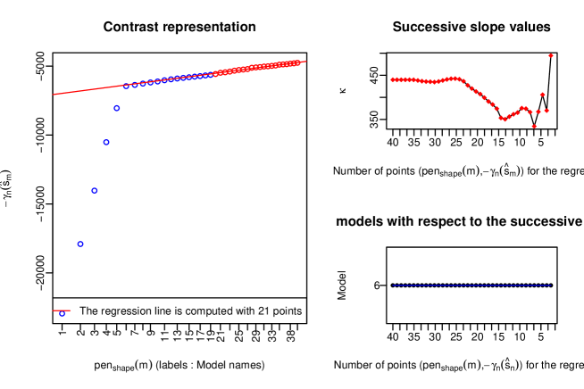
Figure 1: Evolution of $-W_{n}(\hat{c}_{k})$ with respect to k (on the left), Slope values as function of the number of points used to estimate the slope (upper right) and selected number of clusters for each number of points used to estimate the slope (bottom right).

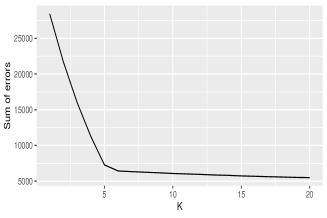
Figure 2: Evolution of $W_{n}(\hat{c}_{k})$ (on the left) and $\text{crit}(k)$ (on the right) with respect to $k$.

As can be seen in figure 1 (left), the last 21 points are used to estimate the regression slope since it behaves like an affine function when k is large. Figure 2 (left) shows that there are two possible elbow of this curve so, the elbow method suggests taking 5 or 6 as the number of clusters. In this case, the elbow method is not ideal. In Figures 3 to 5, in order to visualize data points in dimensions higher than $3$, we represent data as curves that we call ”profiles”, gathered it by cluster, and represented the centers of the groups in red. We also represent the 2 first principal components of the data using robust principal component analysis components (RPCA) (Cardot and Godichon-Baggioni,, 2017). In Figure 3, we focus on the clustering obtained with K-medians algorithm (”Offline” version) for non contaminated data. In each cluster, the curves are close to each other and also close to the median, and the profiles differ from one cluster to another, meaning that our method separated well the 6 groups. In order to visualize the robustness of the proposed method, we consider contaminated data with the law $Z=(Z_{1},...,Z_{5})$ where $Z_{i}$ are i.i.d, with $Z_{i}\sim\mathcal{T}_{1}$ where $\mathcal{T}_{1}$ is a Student law with 1 degree of freedom. Applying our method for selecting the number of clusters for K-medians algorithms, we selected the corrected number of clusters. Furthermore, the obtained groups, up to the presence of some outliers in each clusters, is coherent. Nevertheless, in the case of K-means clustering, the method found non homogeneous clusters, i.e. the method assimilates some far outliers as single clusters (see Figure 5. Note that in the case of contaminated data (Figures 4 and 5), we only represented $95\%$ of the data in order to better visualize them. Then, in Figure, 5, Clusters 5, 7, 8, 11 and 12 are not visible since they are ”far” outliers.

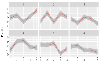
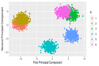
Figure 3: Profiles (on the left) and clustering via K-medians represented on the first two principal components (on the right) without contaminated data.

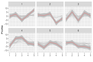
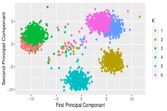
Figure 4: Profiles (on the left) and clustering via K-medians algorithm represented on the first two principal components (on the right) with $5\%$ of contaminated data.

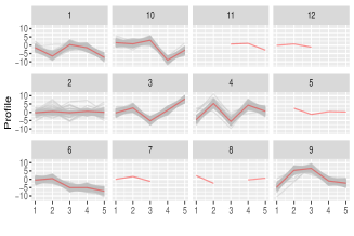
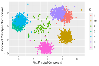
Figure 5: Profiles (on the left) and clustering via K-means algorithm represented on the first two principal components (on the right) with $5\%$ of contaminated data.

4.2 Comparison with Gap Statistic and Silhouette

In what follows, we focus on the choice of the number of clusters and compare our results with different methods. For this, we generated some basic data sets in three different scenarios (see Fischer, (2011)) :
(S1) A single cluster in dimension $10$ : We consider 2000 points uniformly distributed over the unit hypercube in dimension 10.
(S2) 4 clusters in dimension $3$ : The data are generated by Gaussian mixture centered at $(0,0,0)$, $(0,2,3)$, $(3,0,-1)$, and $(-3,-1,0)$ with variance equal to the identity matrix. Each cluster contains 500 data points.
(S3) 5 clusters in dimension $4$ : The data are generated by Gaussian mixture centered at $(0,0,0,0)$, $(3,5,-1,0)$, $(-5,0,0,0)$, $(1,1,6,-2)$ and $(1,-3,-2,5)$ with variance equal to the identity matrix. Each cluster contains 500 data points.

We applied three different methods for determining the number of clusters : the proposed slope method, Gap Statistic and Silhouette method. For each method, we use four clustering algorithms : K-medians (”Online”, ”Semi-Online”, ”Offline”) and K-means. For each scenario, we contaminated our data with the law $Z=(Z_{1},...,Z_{d})$ where $Z_{i}$ are i.i.d, with $Z_{i}\sim\mathcal{T}_{1}$ where $\mathcal{T}_{1}$ is a Student law with 1 degree of freedom. Then, we evaluate our method for the different methods and scenarios by considering:

• N : number of times we get the right value of cluster in 50 repeated trials without contaminated data.

• $\bar{k}$ : average of number of clusters obtained over 50 trials without contaminated data.

• $N_{0.1}$ : number of times we get the right value of cluster in 50 repeated trials with $10\%$ of contaminated data.

• $\bar{k}_{0.1}$ : average of number of clusters obtained over 50 trials with $10\%$ of contaminated data.

Simulations		S1				S2				S3
	Algorithms	$N$	$\bar{k}$	$N_{0.1}$	$\bar{k}_{0.1}$	$N$	$\bar{k}$	$N_{0.1}$	$\bar{k}_{0.1}$	$N$	$\bar{k}$	$N_{0.1}$	$\bar{k}_{0.1}$
Slope	Offline	50	1	49	1.04	50	4	50	4	50	5	50	5
	Semi-Online	46	1.1	44	1.7	50	4	49	4.02	50	5	46	5.1
	Online	43	1.6	49	1.1	48	4	42	4	50	5	40	5.2
	K-means	18	1.6	0	7	50	4	1	7.9	50	5	2	6.7
Gap	Offline	50	1	50	1	6	1.7	0	1	47	4.8	2	1.2
	Semi-Online	50	1	50	1	7	1.7	0	1	47	4.8	2	1.2
	Online	50	1	50	1	8	2.4	0	1	47	4.8	2	1.2
	K-means	50	1	50	1	0	1.2	0	1.2	12	2	0	1.3
Silhouette	Offline	0	6.4	0	2	0	3	0	2.9	24	4.4	1	3.5
	Semi-Online	0	5.8	0	2	0	3	0	2.9	24	4.4	1	3.5
	Online	0	2.1	0	2.1	0	3	2	3.2	27	4.5	2	4.5
	K-means	0	7.9	0	2.1	0	3	7	3.2	27	4.5	0	6.7

Table 1: Comparison of the number of times we get the right value of clusters and the averaged selected number of clusters obtained with the different methods without contaminated data and with $10\%$ of contaminated data.

In case of well separated clusters as in the scenario (S3), the gap statistics method and silhouette method give competitive results. Nevertheless, for closer clusters, the slope method works much better than gap statistics and silhouette method as in the scenario (S2). The gap statistics method works well in scenario 1 in both cases but it works via bootstrapping so it is huge in terms of computation time. Remark that the silhouette method is only defined as $k\geq 2$, explaining partially the bad results for scenario 1. Nevertheless, the silhouette method only works in scenario 3 and is globally not very competitive with the slope method, especially in case of contaminated data. In scenarios 2 and 3 with slope method, Offline, Semi-Online, Online and K-means give better results but in case of contamination, K-means crashes completely while the three other methods seem to be not too much sensitive.

In every scenario, Offline, Semi-Online, Online K-medians with the slope method give very competitive results and in the case where the data are contaminated, they clearly over perform other methods (especially the Offline method).

4.3 Contaminated Data

We now focus on the impact of contaminated data on K-means and K-medians clustering and on the choice of the number of clusters. In this aim, we generate data with a Gaussian mixture model with 10 classes in dimension 5 (whose centers are generated randomly on the sphere of radius $10$) and each class contains 500 data points. The data are contaminated with the law $Z=(Z_{1},...,Z_{5})$ where $Z_{i}$ are i.i.d, with 3 possible scenarios:

1. $Z_{i}\sim\mathcal{T}_{1}$

2. $Z_{i}\sim\mathcal{T}_{2}$

3. $Z_{i}\sim\mathcal{U}[-10,10]$

where $\mathcal{T}_{m}$ is the Student law with m degrees of freedom and $\mathcal{U}[a,b]$ is the continuous uniform distribution on $[a,b]$. In what follows, let us denote by $\rho$ the proportion of contaminated data. In order to compare the different clustering results, we focus on the Adjusted Rand Index (ARI) (Rand,, 1971; Hubert and Arabie,, 1985) which is a measure of similarity between two clusterings and which relies on taking into account the right number of correctly classified pairs. We evaluate for each scenario the average of the number of clusters obtained on 50 trials and the averaged ARI only evaluated on uncontaminated data.

	$\rho$		0	0.01	0.02	0.03	0.05	0.09	0.16	0.28	0.5
$Z_{i}\sim\mathcal{T}_{1}$	Offline	$\bar{k}$	10	10	10.2	10.2	10.7	10.8	11.4	9.9	3.1
	Semi-Online		10	10.1	10.2	10.7	11	11.2	12	10.6	3.2
	Online		10	10.1	10.2	10.8	11.1	11.7	12.1	11.2	2.8
	K-means		10.6	13.5	14	13.6	12.9	12.3	8.9	8.5	11.5
	Offline	ARI	0.99	0.99	0.98	0.99	0.98	0.98	0.97	0.81	0.15
	Semi-Online		0.99	0.99	0.98	0.98	0.98	0.97	0.97	0.91	0.19
	Online		0.99	0.99	0.98	0.98	0.98	0.98	0.97	0.87	0.16
	K-means		0.98	0.94	0.92	0.88	0.79	0.69	0.5	0.33	0.12
$Z_{i}\sim\mathcal{T}_{2}$	Offline	$\bar{k}$	10	10	10.7	11	11	10.9	10.9	11.2	11.1
	Semi-Online		10	10	10.9	11	11	10.9	10.9	11.2	11.1
	Online		10	10.1	11.3	11	11	10.9	10.9	11.2	11.2
	K-means		10.6	11.1	11.5	11.3	11.7	12.1	13	12.7	8
	Offline	ARI	0.99	0.99	0.97	0.98	0.97	0.98	0.98	0.97	0.96
	Semi-Online		0.99	0.99	0.97	0.98	0.97	0.98	0.98	0.97	0.96
	Online		0.99	0.99	0.97	0.98	0.97	0.98	0.98	0.97	0.96
	K-means		0.98	0.98	0.97	0.98	0.97	0.96	0.96	0.95	0.68
$Z_{i}\sim\mathcal{U}[-10,10]$	Offline	$\bar{k}$	10	10	10.1	10.1	10	10	10.5	11.9	10.8
	Semi-Online		10	10	10.1	10.1	10	10	10.3	11.9	10.8
	Online		10	10	10.1	10.1	10	10	10.5	11.1	11.2
	K-means		10.6	10.7	11.1	11.2	12	11.6	11.8	11.3	9.2
	Offline	ARI	0.99	0.99	0.97	0.98	0.97	0.98	0.98	0.97	0.96
	Semi-Online		0.99	0.99	0.97	0.98	0.97	0.98	0.98	0.97	0.96
	Online		0.99	0.99	0.97	0.98	0.97	0.98	0.98	0.97	0.96
	K-means		0.98	0.97	0.97	0.98	0.97	0.96	0.96	0.92	0.79

Table 2: Comparison of the selected number of clusters and the averaged ARI obtained with the different methods with respect to the proportion of contaminated data for $Z_{i}\sim\mathcal{T}_{1}$, $Z_{i}\sim\mathcal{T}_{2}$ and $Z_{i}\sim\mathcal{U}[-10,10]$.

Without contaminated data, the three K-medians algorithms as well as the K-means algorithm have globally found the right number of clusters with an averaged ARI close to $0.99$. Nevertheless, in the case where the data are contaminated by Student’s law with 1 degree of freedom, the proposed slope method for K-medians successfully found more or less the optimal number of clusters up to $28\%$ contamination, and so with competitive ARI, but with $50\%$ contamination it fails to get out of it (logically, since it has a breakdown point at 0.5). Concerning the K-means algorithm, the number of clusters as well as the ARI quickly ”diverge” as the contamination increases, leading, for the case where respectively $2\%$ and $16\%$ of the data are contaminated by a Student with 1 degree of freedom, to respectively $14$ selected clusters and an ARI close to $0.5$.

In the other 2 cases of contamination, K-medians with slope heuristic manages well to find the right number of clusters (fluctuating between $10$ and $11$ essentially) while for K-means, the selected number of clusters fluctuates between $8$ and $13$. Note that in case of high contamination rate, we usually get $11$ clusters, which is logical since most of the contaminated data forms a kind of new cluster around the center of the sphere. In all scenarios, we obtain a better ARI compared to K-means clustering and in terms of ARI, Offline, Semi-Online and Online K-medians algorithms have analogous performances.

We now define the empirical $L^{1}$-error of the centroids estimation by:

$$\sum_{j=1}^{\hat{k}}\min_{j=1,..,k}\left\|\hat{c}_{i}-c_{j}\right\|$$ (2)

with $c=\left\{c_{1},...,c_{k}\right\}$ and $\hat{c}=\left\{\hat{c}_{1},...,\hat{c}_{\hat{k}}\right\}$ where $\hat{k}$ selected number of clusters. The empirical $L^{1}$-error of the centroid estimation and the selected number of clusters, for each algorithms, are given in Figure 6 and 7. In Figure 7 (left), only the K-medians algorithms is visible since the empirical $L^{1}$-error of the centroid estimation of K-means algorithm totally blows up and varies between the values $10000$ and $30000$ with a median close to $15000$. The K-means algorithm is clearly affected by the presence of outliers and both its $L^{1}$-error and its predicted number of clusters are now much larger than for the other algorithms. Other three K-medians algorithms have analogous performances, even if Offline is slightly better.

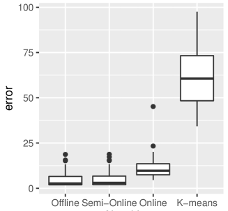
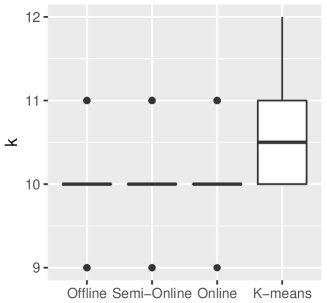
Figure 6: Box plots reflect empirical $L^{1}$-error (see (2)) of centroid estimation (on the left) and the selected number of clusters k (on the right) for the ”Offline”, ”Semi-Online”, ”Online” and K-means without contaminated data.

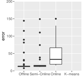
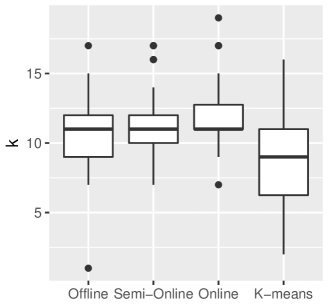
Figure 7: Box plots reflect empirical $L^{1}$-error (see (2)) of centroid estimation (on the left) and the selected number of clusters k (on the right) for the ”Offline”, ”Semi-Online”, ”Online” and K-means with $28\%$ of contaminated data.

4.4 Conclusion

Selecting the number of clusters for K-medians with the proposed penalized criterion calibrated with the help of the slope heuristic method gives very competitive results, and so, even in the presence of outliers (contrary to K-means algorithm). Furthermore, Offline, Semi-Online and Online K-medians algorithms have generally analogous performances even if Offline is slightly better but in terms of computation time, one could prefer Online K-medians in case of large sample. As mentioned in Section 2, one should use the Offline algorithm in case of moderate sample size, the Semi-Online one for medium sample size and finally the Online one for large sample size.

5 Proofs

The proof of the Theorem 1 is inspired by the proof of Theorem 3 in Linder, (2000). Theorem 2 is an adaptation of Theorem 8.1 in Massart, (2007) and Theorem 2.1 in Fischer, (2011).

5.1 Proof of Theorem 3.1

Proof.

For any $c\in S_{k}$, let $T_{n}^{(c)}=\frac{n}{2}(W(c)-W_{n}(c))$ $=\frac{1}{2}\sum_{i=1}^{n}(\mathbb{E}\left[\min_{j=1,..,k}\left\|X_{i}-c_{j}\right\|\right]-\min_{j=1,..,k}\left\|X_{i}-c_{j}\right\|).$
So

$$\mathbb{E}\left[\sup_{c\in S_{k}}(W(c)-W_{n}(c))\right]=\frac{2}{n}\mathbb{E}\left[\sup_{c\in S_{k}}T_{n}^{(c)}\right].$$

Let us first demonstrate that the family of random variables $\left\{T_{n}^{(c)}:c\in S_{k}\right\}$ is subgaussian and sample continuous in a suitable metric. For any $c,c^{\prime}\in S_{k}$ define

$$p(c,c^{\prime})=\sup_{\|x\|\leq R}\left\{\big{|}\min_{j=1,..,k}\left\|x-c_{j}\right\|-\min_{j=1,..,k}\left\|x-c^{\prime}_{j}\right\|\hskip 2.84526pt\big{|}\right\}$$

and $p_{n}(c,c^{\prime})=\sqrt{n}p(c,c^{\prime})$, $p_{n}$ is a metric on $S_{k}$. Since we have,

$$\big{|}T_{n}^{(c)}-T_{n}^{(c^{\prime})}\big{|} =\frac{n}{2}\big{|}W(c)-W(c^{\prime})+W_{n}(c^{\prime})-W_{n}(c)\big{|}$$

$$\leq\frac{n}{2}\left(\big{|}W(c)-W(c^{\prime})\big{|}+\big{|}W_{n}(c^{\prime})-W_{n}(c)\big{|}\right)$$

$$\leq np(c,c^{\prime})=\sqrt{n}p_{n}(c,c^{\prime})$$

and the family $\left\{T_{n}^{(c)}:c\in S_{k}\right\}$ is then sample continuous in the metric $p_{n}$. To show that $\left\{T_{n}^{(c)}:c\in S_{k}\right\}$ is subgaussian in $p_{n}$, let

$$Y_{i}=\frac{1}{2}\left(W(c)-\min_{j=1,..,k}\left\|x-c_{j}\right\|\right)-\frac{1}{2}\left(W(c^{\prime})-\min_{j=1,..,k}\left\|x-c^{\prime}_{j}\right\|\right).$$

Then

$$T_{n}^{(c)}-T_{n}^{(c^{\prime})}=\sum_{i=1}^{n}Y_{i}$$

where $Y_{i}$ are independent, have zero mean, and

$$\big{|}Y_{i}\big{|}\leq\frac{1}{\sqrt{n}}p_{n}(c,c^{\prime}).$$

By Lemma 5.1, we obtain

$$\mathbb{E}\left[e^{\lambda(T_{n}^{(c)}-T_{n}^{(c^{\prime})})}\right]\leq e^{\frac{\lambda^{2}p_{n}(c,c^{\prime})^{2}}{2}}.$$

So, $\left\{T_{n}^{(c)}:c\in S_{k}\right\}$ is subgaussian in $p_{n}$. As the family $\left\{T_{n}^{(c)}:c\in S_{k}\right\}$ is subgaussian and sample continuous in $p_{n}$, Lemma 5.2 gives

$$\mathbb{E}\left[\sup_{c\in S_{k}}T_{n}^{(c)}\right]\leq 12\int_{0}^{\text{diam}(S_{k})/2}\sqrt{\ln{N_{p_{n}}(S_{k},\epsilon)}}d\epsilon.$$

By Lemma 5.4, we obtain

$$N_{p_{n}}(S_{k},\epsilon)\leq\left(\frac{4R\sqrt{n}}{\epsilon}\right)^{kd}$$

and since $\text{diam}(S_{k})\leq\sqrt{n}2R$

$$\mathbb{E}\left[\sup_{c\in S_{k}}T_{n}^{(c)}\right] \leq\frac{24}{n}\int_{0}^{\sqrt{n}R}\sqrt{\ln\left(\left({\frac{4R\sqrt{n}}{\epsilon}}\right)^{kd}\right)}d\epsilon$$

$$=\frac{24\sqrt{kd}}{n}\int_{0}^{\sqrt{n}R}\sqrt{\ln\left({\frac{4R\sqrt{n}}{\epsilon}}\right)}d\epsilon.$$

Considering $x=\frac{\epsilon}{4R\sqrt{n}}$, we obtain,

$$\mathbb{E}\left[\sup_{c\in S_{k}}T_{n}^{(c)}\right]\leq\frac{24\sqrt{kd}}{n}\int_{0}^{\frac{1}{4}}4R\sqrt{n}\sqrt{\ln\left({\frac{1}{x}}\right)}dx.$$

Applying Jensen’s inequality to the concave function $f(x)=\sqrt{x}$ :

$$\mathbb{E}\left[\sup_{c\in S_{k}}T_{n}^{(c)}\right] \leq 24R\sqrt{\frac{kd}{n}}\sqrt{\int_{0}^{\frac{1}{4}}4\ln\left({\frac{1}{x}}\right)dx}$$

$$=24R\sqrt{\frac{kd}{n}}\sqrt{1+\ln{4}}$$

$$\leq 48R\sqrt{\frac{kd}{n}}$$

where we used that $\int\ln{x}=x\ln{x}-x$ and $\ln{4}\leq 3$.
Thus,

$$\mathbb{E}\left[\sup_{c\in S_{k}}\left\{W(c)-W_{n}(c)\right\}\right]\leq 48R\sqrt{\frac{kd}{n}}.$$

∎

5.2 Proof of Theorem 3.2

Proof.

By definition of $\tilde{c},$ for all $k,1\leq k\leq n$ and $c_{k}\in S_{k}$, we have:

$$W_{n}(\tilde{c})+\text{pen}(\hat{k})\leq W_{n}(c_{k})+\text{pen}(k)$$

$$W(\tilde{c})\leq W_{n}(c_{k})+W(\tilde{c})-W_{n}(\tilde{c})+\text{pen}(k)-\text{pen}(\hat{k}).$$ (3)

Consider nonnegative weights $\left\{x_{l}\right\}_{1\leq l\leq n}$ such that $\sum_{l=1}^{n}e^{-x_{l}}=\Sigma$ and let z $>$ 0.
Applying Lemma 5.5 with $f(x)=\frac{1}{n}\min_{j=1,..,l}\left\|x-c_{j}\right\|$, $a=0$ and $b=\frac{2R}{n}$ for all $l,1\leq l\leq n$ and all $\epsilon_{l}>0$

$$\mathds{P}\left[\sup_{c\in S_{l}}(W(c)-W_{n}(c))-\mathbb{E}\left[\sup_{c\in S_{l}}(W(c)-W_{n}(c))\right]\geq\epsilon_{l}\right]\leq\exp\left(-\frac{n\epsilon_{l}^{2}}{2R^{2}}\right).$$

It follows that for all l, taking $\epsilon_{l}=2R\sqrt{\frac{x_{l}+z}{2n}}$

$$\mathds{P}\left[\sup_{c\in S_{l}}(W(c)-W_{n}(c))\geq\mathbb{E}\left[\sup_{c\in S_{l}}(W(c)-W_{n}(c))\right]+2R\sqrt{\frac{x_{l}+z}{2n}}\right]\leq e^{-x_{l}-z}.$$

Thus, we have

$$\mathds{P}\left[\bigcap_{l=1}^{n}\sup_{c\in S_{l}}(W(c)-W_{n}(c))\leq\mathbb{E}\left[\sup_{c\in S_{l}}(W(c)-W_{n}(c))\right]+2R\sqrt{\frac{x_{l}+z}{2n}}\right]$$

$$=1-\mathds{P}\left[\bigcup_{l=1}^{n}\sup_{c\in S_{l}}(W(c)-W_{n}(c))\geq\mathbb{E}\left[\sup_{c\in S_{l}}(W(c)-W_{n}(c))\right]+2R\sqrt{\frac{x_{l}+z}{2n}}\right]\geq 1-\Sigma e^{-z}.$$

Considering $Z_{l}=\mathbb{E}\left[\sup_{c\in S_{l}}(W(c)-W_{n}(c))\right]$, let us show if we have for all $1\leq l\leq n$,

$$\sup_{c\in S_{l}}(W(c)-W_{n}(c))\leq Z_{l}+2R\sqrt{\frac{x_{l}+z}{2n}}$$

then,

$$W(\tilde{c})\leq W_{n}(c_{k})+2R\sqrt{\frac{z}{2n}}+\text{pen}(k).$$

We suppose that we have

$$\sup_{c\in S_{l}}(W(c)-W_{n}(c))\leq Z_{l}+2R\sqrt{\frac{x_{l}+z}{2n}}\hskip 28.45274pt\forall 1\leq l\leq n$$ (4)

Particularly it’s true for $l=\hat{k}$, we have also $W(\tilde{c})-W_{n}(\tilde{c})\leq\sup_{c\in S_{\hat{k}}}(W(c)-W_{n}(c))$ and $\sqrt{a+b}\leq\sqrt{a}+\sqrt{b}$ $\forall a,b\geq 0$. By combining this result with (2) and (3), we get

$$W(\tilde{c}) \leq W_{n}(c_{k})+\sup_{c\in S_{\hat{k}}}(W(c)-W_{n}(c))+\text{pen}(k)-\text{pen}(\hat{k})$$

$$\leq W_{n}(c_{k})+Z_{\hat{k}}+2R\sqrt{\frac{x_{\hat{k}}}{2n}}+2R\sqrt{\frac{z}{2n}}+\text{pen}(k)-\text{pen}(\hat{k}).$$

With the help of Theorem 3.2, we have $Z_{k}\leq 48R\sqrt{\frac{kd}{n}}$ for all $k,1\leq k\leq n$ and if we have $\text{pen}(k)\geq R\left(48\sqrt{\frac{kd}{n}}+2\sqrt{\frac{x_{k}}{2n}}\right)$

$$W(\tilde{c}) \leq W_{n}(c_{k})+48R\sqrt{\frac{\hat{k}d}{n}}+2R\sqrt{\frac{x_{\hat{k}}}{2n}}+2R\sqrt{\frac{z}{2n}}+\text{pen}(k)-R\left(48\sqrt{\frac{\hat{k}d}{n}}+2\sqrt{\frac{x_{\hat{k}}}{2n}}\right)$$

$$=W_{n}(c_{k})+2R\sqrt{\frac{z}{2n}}+\text{pen}(k)$$

which shows that

$$W(\tilde{c})\leq W_{n}(c_{k})+2R\sqrt{\frac{z}{2n}}+\text{pen}(k).$$

Thus

$$\mathds{P}\left[W(\tilde{c})\leq W_{n}(c_{k})+2R\sqrt{\frac{z}{2n}}+\text{pen}(k)\right]$$

$$\geq\mathds{P}\left[\bigcap_{l=1}^{n}\sup_{c\in S_{l}}(W(\mu,c)-W(\mu_{n},c))\leq\mathbb{E}\left[\sup_{c\in S_{l}}(W(c)-W_{n}(c))\right]+2R\sqrt{\frac{x_{l}+z}{2n}}\right]\geq 1-\Sigma e^{-z}.$$

We get

$$\mathds{P}\left[W(\tilde{c})-W_{n}(c_{k})-\text{pen}(k)\geq 2R\sqrt{\frac{z}{2n}}\right]\leq\Sigma e^{-z}$$

$$\mathds{P}\left[\frac{\sqrt{2n}}{2R}(W(\tilde{c})-W_{n}(c_{k})-\text{pen}(k))\geq\sqrt{z}\right]\leq\Sigma e^{-z}$$

or, setting $z=u^{2}$,

$$\mathds{P}\left[\frac{\sqrt{2n}}{2R}(W(\tilde{c})-W_{n}(c_{k})-\text{pen}(k))\geq u\right]\leq\Sigma e^{-u^{2}}$$

$$\mathbb{E}\left[\frac{\sqrt{2n}}{2R}(W(\tilde{c})-W_{n}(c_{k})-\text{pen}(k))_{+}\right] =\int_{0}^{\infty}\mathds{P}\left[\frac{\sqrt{2n}}{2R}(W(\tilde{c})-W_{n}(c_{k})-\text{pen}(k))_{+}\geq u\right]du$$

$$\leq\int_{0}^{\infty}\mathds{P}\left[\frac{\sqrt{2n}}{2R}(W(\tilde{c})-W_{n}(c_{k})-\text{pen}(k))\geq u\right]du$$

$$\leq\Sigma\int_{0}^{\infty}e^{-u^{2}}du=\Sigma\frac{\sqrt{\pi}}{2}.$$

We get

$$\mathbb{E}\left[(W(\tilde{c})-W_{n}(c_{k})-\text{pen}(k))_{+}\right]\leq\Sigma R\sqrt{\frac{\pi}{2n}}.$$

Since $\mathbb{E}\left[W_{n}(c_{k})\right]=W(c_{k})$, we have :

$$\mathbb{E}\left[W(\tilde{c})\right]\leq W(c_{k})+\text{pen}(k)+\Sigma R\sqrt{\frac{\pi}{2n}}.$$

$$\mathbb{E}\left[W(\tilde{c})\right]\leq\inf_{1\leq k\leq n,c_{k}\in S_{k}}\left\{W(c_{k})+\text{pen}(k)\right\}+\Sigma R\sqrt{\frac{\pi}{2n}}.$$

∎

5.3 Proof of Proposition 3.1

Proof.

If $k\leq 2^{d}$, we have $4Rk^{-1/d}\geq 4R2^{-1}=2R$. Thus, $W(c)\leq 2\sqrt{d}\leq 4\sqrt{d}k^{-1/d}$ for any vector quantizer with codebook c.
Otherwise, let $\epsilon=4Rk^{-1/d}$. Then $\epsilon\leq 2R$ and by Lemma 5.3 there exists a set of points $\left\{y_{1},...,y_{k}\right\}\subset S(0,R)$ that $\epsilon$-covers $S(0,R)$. A quantizer with the codebook $c=\left\{y_{1},...,y_{k}\right\}$ verifies :

$$W(c)\leq\epsilon\leq 4Rk^{-1/d}$$

That concludes

$$\inf_{c\in S_{k}}W(c)\leq 4Rk^{-1/d}$$

∎

5.4 Some definitions and lemma

These are some definitions and lemma that are useful to prove these theorems.

Definitions :

• Let (S,p) be a totally bounded metric space. For any $F\subset S$ and $\epsilon>0$ the $\epsilon$-covering number $N_{p}(F,\epsilon)$ of F is defined as the minimum number of closed balls with radius $\epsilon$ whose union covers F.

• A Family $\left\{T_{s}:s\in S\right\}$ of zero-mean random variables indexed by the metric space (S, p) is called subgaussian in the metric p if for any $\lambda>0$ and $s,s^{\prime}\in S$ we have

  $$\mathbb{E}\left[e^{\lambda(T_{s}-T_{s^{\prime}})}\right]\leq e^{\frac{\lambda^{2}p(s,s^{\prime})^{2}}{2}}$$

• The Family $\left\{T_{s}:s\in S\right\}$ is called sample continuous if for any sequence $s_{1},s_{2}..,\in S$ such that $s_{j}\rightarrow s\in S$ we have $T_{s_{j}}\rightarrow T_{s}$ with probability one.

Lemma 5.1 (Hoeffding, (1994)).

Let $Y_{1},..,Y_{n}$ are independent zero-mean random variables such that $a\leq Y_{i}\leq b,i=1,...,n$, then for all $\lambda>0$,

$$\mathbb{E}\left[e^{\lambda(\sum_{i=1}^{n}Y_{i})}\right]\leq e^{\frac{\lambda^{2}n(b-a)^{2}}{8}}$$

Lemma 5.2 (Cesa-Bianchi and Lugosi, (1999), Proposition 3).

If $\left\{T_{s}:s\in S\right\}$ is subgaussian and sample continuous in the metric p, then

$$\mathbb{E}\left[\sup_{s\in S}T_{s}\right]\leq 12\int_{0}^{\text{diam}(S)/2}\sqrt{\ln{N_{p}(S,\epsilon)}}d\epsilon$$

Lemma 5.3 (Bartlett et al., (1998), Lemma 1).

Let S(0,r) denote the closed d-dimensional sphere of radius r centered at x. Let $\epsilon>0$ and $N(\epsilon)$ denote the cardinality of the minimum $\epsilon$ covering of $S(0,r)$, that is, $N(\epsilon)$ is the smallest integer N such that there exist points $\left\{y_{1},...,y_{N}\right\}\subset S(0,r)$ with the property

$$\sup_{x\in S(0,r)}\min_{1\leq i\leq N}\left\|x-y_{i}\right\|\leq\epsilon$$

Then, for all $\epsilon\leq 2r$ we have

$$N(\epsilon)\leq\left(\frac{4r}{\epsilon}\right)^{d}$$

Lemma 5.4.

For any $0<\epsilon<2R$ and $k\geq 1$, the covering number of $S_{k}$ in the metric

$$p(c,c^{\prime})=\sup_{\|x\|\leq R}\left\{\big{|}\min_{j=1,..,k}\left\|x-c_{j}\right\|-\min_{j=1,..,k}\|x-c^{\prime}_{j}\|\hskip 2.84526pt\big{|}\right\}$$

is bounded as

$$N_{p}(S_{k},\epsilon)\leq\left(\frac{4R}{\epsilon}\right)^{kd}.$$

Proof of the Lemma 4 : .

Let $0<\epsilon\leq 2R$ by Lemma 3 there exists a $\epsilon$-covering set of points $\left\{y_{1},...,y_{N}\right\}\subset S(0,R)$ with $N\leq\left(\frac{4R}{\epsilon}\right)^{d}$.
Since, we have $N^{k}$ ways to choose k codepoints from a set of N points $\left\{y_{1},...,y_{N}\right\}$, that implies

$$N_{p}(S_{k},\epsilon)\leq\left(\frac{4R}{\epsilon}\right)^{kd}.$$

For any codepoints $\left\{c_{1},...,c_{k}\right\}$ which are contained in $S(0,R)$, there exists a set of codepoints such that $\left\|c_{j}-c^{\prime}_{j}\right\|\leq\epsilon$ for all j.
Let us first show

$$\min_{j=1,..,k}\left\|x-c_{j}\right\|-\min_{j=1,..,k}\left\|x-c^{\prime}_{j}\right\|\leq\epsilon.$$

In this aim, let us consider $q\in\arg\min_{j=1,..,k}\left\|x-c_{j}\right\|$, then

$$\min_{j=1,..,k}\left\|x-c^{\prime}_{j}\right\|-\min_{j=1,..,k}\left\|x-c_{j}\right\|\leq\left\|x-c^{\prime}_{q}\right\|-\left\|x-c_{q}\right\|\leq\left\|c_{q}-c^{\prime}_{q}\right\|\leq\epsilon.$$

In the same way, considering $q^{\prime}\in\arg\min_{j=1,..,k}\left\|x-c^{\prime}_{j}\right\|$ , we show

$$\min_{j=1,..,k}\left\|x-c_{j}\right\|-\min_{j=1,..,k}\left\|x-c^{\prime}_{j}\right\|\leq\left\|x-c_{q^{\prime}}\right\|-\left\|x-c^{\prime}_{q^{\prime}}\right\|\leq\left\|c_{q^{\prime}}-c^{\prime}_{q^{\prime}}\right\|\leq\epsilon.$$

So,

$$\big{|}\min_{j=1,..,k}\left\|x-c_{j}\right\|-\min_{j=1,..,k}\left\|x-c^{\prime}_{j}\right\|\hskip 2.84526pt\big{|}\leq\epsilon$$

for any codepoints $\left\{c_{1},...,c_{k}\right\}$ which are contained in $S(0,R)$, there exists a set of codepoints $\left\{c^{\prime}_{1},...,c^{\prime}_{k}\right\}$ such that

$$\big{|}\min_{j=1,..,k}\left\|x-c_{j}\right\|-\min_{j=1,..,k}\left\|x-c^{\prime}_{j}\right\|\hskip 2.84526pt\big{|}\leq\epsilon.$$

∎

Lemma 5.5 (McDiarmid et al., (1989), Massart, (2007) : Theorem 5.3).

If $X_{1},...X_{n}$ are independent random variables and $\mathcal{F}$ is a finite or countable class of real-valued functions such that $a\leq f\leq b$ for all $f\in\mathcal{F}$, the if $Z=\sup_{f\in\mathcal{F}}\sum_{i=1}^{n}(f(X_{i})-\mathbb{E}\left[f(X_{i})\right])$, we have, for every $\epsilon>0$,

$$\mathds{P}\left[Z-\mathbb{E}\left[Z\right]\geq\epsilon\right]\leq\exp\left(-\frac{2\epsilon^{2}}{n(b-a)^{2}}\right)$$

References

- Arlot and Massart, (2009) Arlot, S. and Massart, P. (2009). Data-driven calibration of penalties for least-squares regression. Journal of Machine learning research, 10(2).
- Bartlett et al., (1998) Bartlett, P. L., Linder, T., and Lugosi, G. (1998). The minimax distortion redundancy in empirical quantizer design. IEEE Transactions on Information theory, 44(5):1802–1813.
- Baudry et al., (2012) Baudry, J.-P., Maugis, C., and Michel, B. (2012). Slope heuristics: overview and implementation. Statistics and Computing, 22(2):455–470.
- Berkhin, (2006) Berkhin, P. (2006). A survey of clustering data mining techniques. In Grouping multidimensional data, pages 25–71. Springer.
- Bezdek, (2013) Bezdek, J. C. (2013). Pattern recognition with fuzzy objective function algorithms. Springer Science & Business Media.
- Birgé and Massart, (2007) Birgé, L. and Massart, P. (2007). Minimal penalties for gaussian model selection. Probability theory and related fields, 138(1):33–73.
- Brault et al., (2011) Brault, V., Baudry, J.-P., Maugis, C., Michel, B., and Brault, M. V. (2011). Package ‘capushe’.
- Cardot et al., (2012) Cardot, H., Cénac, P., and Monnez, J.-M. (2012). A fast and recursive algorithm for clustering large datasets with k-medians. Computational Statistics & Data Analysis, 56(6):1434–1449.
- Cardot et al., (2013) Cardot, H., Cénac, P., and Zitt, P.-A. (2013). Efficient and fast estimation of the geometric median in hilbert spaces with an averaged stochastic gradient algorithm. Bernoulli, 19(1):18–43.
- Cardot and Godichon-Baggioni, (2017) Cardot, H. and Godichon-Baggioni, A. (2017). Fast estimation of the median covariation matrix with application to online robust principal components analysis. Test, 26(3):461–480.
- Cesa-Bianchi and Lugosi, (1999) Cesa-Bianchi, N. and Lugosi, G. (1999). Minimax regret under log loss for general classes of experts. In Proceedings of the Twelfth annual conference on computational learning theory, pages 12–18.
- Cheng, (1995) Cheng, Y. (1995). Mean shift, mode seeking, and clustering. IEEE transactions on pattern analysis and machine intelligence, 17(8):790–799.
- Dempster et al., (1977) Dempster, A. P., Laird, N. M., and Rubin, D. B. (1977). Maximum likelihood from incomplete data via the em algorithm. Journal of the Royal Statistical Society: Series B (Methodological), 39(1):1–22.
- Duflo, (1997) Duflo, M. (1997). Random iterative models, stochastic modelling and applied probability, vol. 34.
- Dunn, (1973) Dunn, J. C. (1973). A fuzzy relative of the isodata process and its use in detecting compact well-separated clusters.
- Ester et al., (1996) Ester, M., Kriegel, H.-P., Sander, J., Xu, X., et al. (1996). A density-based algorithm for discovering clusters in large spatial databases with noise. In kdd, volume 96, pages 226–231.
- Fischer, (2011) Fischer, A. (2011). On the number of groups in clustering. Statistics & Probability Letters, 81(12):1771–1781.
- Forgy, (1965) Forgy, E. W. (1965). Cluster analysis of multivariate data: efficiency versus interpretability of classifications. biometrics, 21:768–769.
- Gagolewski et al., (2016) Gagolewski, M., Bartoszuk, M., and Cena, A. (2016). Genie: A new, fast, and outlier-resistant hierarchical clustering algorithm. Information Sciences, 363:8–23.
- Gersho and Gray, (2012) Gersho, A. and Gray, R. M. (2012). Vector quantization and signal compression, volume 159. Springer Science & Business Media.
- Haldane, (1948) Haldane, J. (1948). Note on the median of a multivariate distribution. Biometrika, 35(3-4):414–417.
- Hartigan, (1975) Hartigan, J. A. (1975). Clustering algorithms. John Wiley & Sons, Inc.
- Hartigan and Wong, (1979) Hartigan, J. A. and Wong, M. A. (1979). Algorithm as 136: A k-means clustering algorithm. Journal of the royal statistical society. series c (applied statistics), 28(1):100–108.
- Hoeffding, (1994) Hoeffding, W. (1994). Probability inequalities for sums of bounded random variables. In The collected works of Wassily Hoeffding, pages 409–426. Springer.
- Hubert and Arabie, (1985) Hubert, L. and Arabie, P. (1985). Comparing partitions. Journal of classification, 2(1):193–218.
- Jain and Dubes, (1988) Jain, A. K. and Dubes, R. C. (1988). Algorithms for clustering data. Prentice-Hall, Inc.
- Jain et al., (1999) Jain, A. K., Murty, M. N., and Flynn, P. J. (1999). Data clustering: a review. ACM computing surveys (CSUR), 31(3):264–323.
- Kaufman and Rousseeuw, (2009) Kaufman, L. and Rousseeuw, P. J. (2009). Finding groups in data: an introduction to cluster analysis. John Wiley & Sons.
- Kemperman, (1987) Kemperman, J. (1987). The median of a finite measure on a banach space. Statistical data analysis based on the L1-norm and related methods (Neuchâtel, 1987), pages 217–230.
- Linder, (2000) Linder, T. (2000). On the training distortion of vector quantizers. IEEE Transactions on Information Theory, 46(4):1617–1623.
- MacQueen, (1967) MacQueen, J. (1967). Classification and analysis of multivariate observations. In 5th Berkeley Symp. Math. Statist. Probability, pages 281–297.
- Massart, (2007) Massart, P. (2007). Concentration inequalities and model selection: Ecole d’Eté de Probabilités de Saint-Flour XXXIII-2003. Springer.
- McDiarmid et al., (1989) McDiarmid, C. et al. (1989). On the method of bounded differences. Surveys in combinatorics, 141(1):148–188.
- Mirkin, (1996) Mirkin, B. (1996). Mathematical classification and clustering, volume 11. Springer Science & Business Media.
- Polyak and Juditsky, (1992) Polyak, B. T. and Juditsky, A. B. (1992). Acceleration of stochastic approximation by averaging. SIAM journal on control and optimization, 30(4):838–855.
- Rand, (1971) Rand, W. M. (1971). Objective criteria for the evaluation of clustering methods. Journal of the American Statistical association, 66(336):846–850.
- Robbins and Monro, (1951) Robbins, H. and Monro, S. (1951). A stochastic approximation method. The annals of mathematical statistics, pages 400–407.
- Ruppert, (1985) Ruppert, D. (1985). A newton-raphson version of the multivariate robbins-monro procedure. The Annals of Statistics, 13(1):236–245.
- Spath, (1980) Spath, H. (1980). Cluster analysis algorithms for data reduction and classification of objects. Ellis Horwood Chichester.
- Tibshirani et al., (2001) Tibshirani, R., Walther, G., and Hastie, T. (2001). Estimating the number of clusters in a data set via the gap statistic. Journal of the Royal Statistical Society: Series B (Statistical Methodology), 63(2):411–423.
- Vardi and Zhang, (2000) Vardi, Y. and Zhang, C.-H. (2000). The multivariate l 1-median and associated data depth. Proceedings of the National Academy of Sciences, 97(4):1423–1426.
- Weiszfeld, (1937) Weiszfeld, E. (1937). Sur le point pour lequel la somme des distances de n points donnés est minimum. Tohoku Mathematical Journal, First Series, 43:355–386.