Variational optimization of tensor-network states with the honeycomb-lattice corner transfer matrix

Abstract

We develop a method of variational optimization of the infinite projected entangled pair states on the honeycomb lattice. The method is based on the automatic differentiation of the honeycomb-lattice corner transfer matrix renormalization group. We apply the approach to the antiferromagnetic Heisenberg spin-1/2 and ferromagnetic Kitaev models on the honeycomb lattice. The developed formalism gives quantitatively accurate results for the main physical observables and has a necessary potential for further extensions.

I Introduction

The most difficult part of any two- or three-dimensional tensor-network algorithm, especially the infinite projected entangled pair states (iPEPS) optimization and calculation of observables with it, is the tensor-network contraction Ran et al. (2020). Exact contraction of the PEPS norm is exponentially hard in general. Therefore, in two-dimensional tensor-network calculations, one requires to contract a tensor network approximately. There are three main methods to contract two-dimensional tensor networks with certain translational invariance: transfer matrix methods, also called the boundary matrix product states Jordan et al. (2008), tensor renormalization group (TRG) Gu et al. (2008); Jiang et al. (2008) including its modifications, and methods based on the corner transfer matrix (CTM) Orús and Vidal (2009). There are also several mixed versions, e.g., the channel environments  Vanderstraeten et al. (2015), which are similar to both CTM and transfer matrix methods.

All the mentioned approaches are most naturally defined for a square lattice geometry, though transfer matrices were also used for kagome and honeycomb lattices Xie et al. (2017), while TRG was applied to the honeycomb lattice Jiang et al. (2008). At the same time, CTM methods, at least in the iPEPS calculations, were mainly applied to the square lattice. The strategy to deal with other lattices was to map it onto the square lattice and then to employ already developed algorithms. This strategy was successfully applied to star- Jahromi and Orús (2018), ruby- Jahromi et al. (2018), kagome- Corboz et al. (2012a), triangular- Bauer et al. (2012) and honeycomb-lattice geometries Corboz et al. (2012b) with the simple or full update as an optimization method for iPEPS.

Still, the most accurate iPEPS optimization method is the variational update. Originally, it was proposed for the square lattice Corboz (2016); Vanderstraeten et al. (2016), where the gradients were derived in terms of the CTM tensors or channel environments. Later, it was observed that the gradients can be derived with the help of automatic differentiation Liao et al. (2019), originally developed in the machine-learning community. In this approach, one needs only to calculate the energy with an approximate contraction scheme by using only differentiable procedures. In particular, it can be applied to the lattices other than square with the help of special mappings of these to the square one Ferrari et al. (2022). The variational approach enables studies of the next-nearest-neighbor (NNN) frustrated systems Hasik et al. (2021) and chiral spin liquids Hasik et al. (2022).

In this paper, we aim to establish whether other efficient contraction methods on other lattices can lead to a stable variational update with gradients derived by the automatic differentiation. We focus on a generalization of the corner transfer matrix renormalization group (CTMRG) approach to the honeycomb-lattice tensor network. We describe the contraction scheme and employ it for the ground-state analysis of the antiferromagnetic Heisenberg model on the honeycomb lattice. We employ the zygote autodifferentiation package Innes (2018) to compute gradients and optimize the iPEPS wave function by using the Broyden-Fletcher-Goldfarb-Shanno (BFGS) algorithm.

It should be noted that CTMRG on lattices other than square, in particular, on hyperbolic lattices Daniška and Gendiar (2015, 2016), were used in the variational calculations with the interaction-round-a-face (IRF) type tensor network as a variational ansatz Nishio et al. (2004). These optimizations were conducted by using the Nelder-Mead method.

II Method and results

II.1 Honeycomb CTMRG

CTM was originally developed by Baxter as a method of exact solution of certain integrable models on the square lattice Baxter (1968, 1978). Later, it was generalized to a triangular lattice Tsang (1977); Baxter and Tsang (1980). Nishino and Okunishi developed CTM into the numerical renormalization group method (CTMRG) Nishino and Okunishi (1996), which was further generalized to the classical statistical mechanics systems on triangular and hyperbolic lattices Ueda et al. (2007); Iharagi et al. (2010); Krcmar et al. (2008); Gendiar et al. (2012); Genzor et al. (2017). Still, their scheme on the triangular lattice was tailored for the IRF-like models, while we are interested in the vertex like model, since the PEPS norm can be represented as a contraction of the vertex model partition function. For this purpose, we dualize the construction from Ref. Gendiar et al. (2012) by obtaining CTMRG for a honeycomb-lattice tensor network from the CTMRG of the IRF classical model on the triangular lattice.

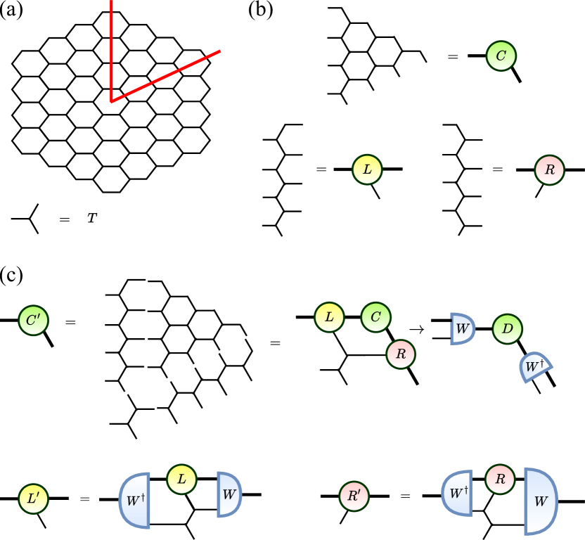
Figure 1: Illustration of the definitions of CTMRG on a honeycomb lattice. (a) A honeycomb lattice can be divided into six corners. Any trivalent vertex of the lattice corresponds to the tensor $T$. (b) Definitions of corner matrix $C$ and two column tensors $L,R$. In the real calculations we assume that these corners and columns contain an infinite number of sites, but the finite equivalents, shown in the figure, can be used as initialization. (Note that the initialization of the matrix $C$ is Hermitian but not diagonal. One can gauge it to the diagonal form, but since we do not introduce any truncations in the initialization, this additional gauge choice has no impact on any further calculations.) (c) Illustration of the update procedure for the matrix $C$ and the tensors $L$ and $R$. This update is repeated until the convergence.

Let us start with a honeycomb lattice characterized by a single trivalent tensor $T$, symmetric under rotations and reflection conjugations, with the bond dimension $D$ on all of its vertices. This lattice can be divided into six corners, which are shown in Fig. 1(a). Contraction of all tensors in the corner can be represented as a matrix $C$ [see Fig. 1(b)]. If the individual tensors are symmetric under rotations and homogeneous around the lattice, then all the corner matrices $C$ are identical and the tensor network contraction $Z$ can be represented as

$$Z=\operatorname{Tr}{C^{6}}.$$ (1)

Additionally, following Ref. Gendiar et al. (2012), we can introduce two row tensors $L$ and $R$, which are also shown in Fig. 1(b). In the infinite system, the tensors $C$, $L$, and $R$ are infinite-dimensional, but in the numerical procedure we can truncate them to a finite dimension by using the spectrum of $C$ as a guide for truncation. We initialize $C$, $L$, and $R$ with their small lattice analogs and increase the lattice by adding lattice sites. In each step of this increase we perform the updates, which are illustrated in Fig. 1(c) and can be expressed as

$$C \to LCRT^{2},$$ (2)

$$L \to LT^{2},$$ (3)

$$R \to RT^{2}.$$ (4)

The updated matrix $C$ has a dimension $\chi D$, where $\chi$ is a dimension of the original matrix $C$. Next, we need to truncate the matrix $C$ back to the original dimension $\chi$. To this end, we diagonalize the matrix $C=WDW^{\dagger}$ and truncate it by using its eigenspectum (note that here the eigenvalues can be negative and must be sorted by the absolute value). The Hermiticity of the matrix $C$ is ensured by the reflection-conjugation symmetry of the original tensors $T$. Alternatively, we can use the singular value decomposition (SVD). After this decomposition, the new matrix $C$ is set as $C=D$, while the matrices $W$ and $W^{\dagger}$ are absorbed into the updated $L$ and $R$ [see also Fig. 1(c)]. Finally, we repeat the lattice increasing process until the convergence. The update of the CTM tensors includes only $\chi$ largest eigenvalues of the decomposition, which can be computed with iterative eigensolvers (or a randomized SVD in case of the SVD decomposition) to reduce the complexity. In the case of the randomized SVD decomposition, the computational complexity scales as $O(D^{4}\chi^{3}+D^{6}\chi^{2})$.

The converged CTM environments enable computation of both local observables and nonlocal correlation functions. Figures 1(a) and 1(b) show tensor contractions, which are used in calculations of the one- and two-site observables. $T_{\rm imp}$ in Fig. 2 corresponds to the impurity tensor similar to the iPEPS double-layer site tensor with a spin operator. To obtain the expectation value of these one- and two-site observables, the tensor contractions in Fig. 2 must be additionally normalized by the same contractions with tensors $T_{\rm imp}$ replaced by $T$. Note that the one-site observable is computed only with the $L$-type tensors. But from the definitions of $L$ and $R$ tensors it follows that these quantities can also be computed only with the $R$-type tensors (or with some combination of $L$ and $R$). For consistency, all these definitions of observables must agree. In practical calculations, this agreement is enforced by the equality schematically depicted in Fig. 2(c). This equality holds to a high accuracy for the converged CTM tensors (the detailed accuracy slightly depends on the choice of parameters in the randomized SVD algorithm). Finally, in our iPEPS calculations we use extrapolation of the results based on the correlation length scaling. Figure 2(d) defines the transfer matrix $E$ with the honeycomb-lattice CTM tensors. The correlation length $\xi$ can be computed from the eigenvalues $\lambda_{i}$ of the transfer matrix $E$ as $\xi=-{1}/{\log{|\lambda_{2}/\lambda_{1}|}}$.

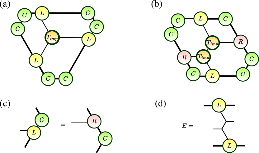
Figure 2: Illustration of computation of different observables with the CTMRG environments on the honeycomb lattice. (a) Calculation of the one-site correlator with the impurity tensor $T_{\rm imp}$, which characterizes a local observable (e.g., the magnetization). (b) Calculation of the two-point correlator with CTMRG environments. (c) Observables can be computed with either $L$ or $R$ tensors and the environments must be equivalent for consistency of the results. (In practice, this equivalence is ensured by the condition shown in the figure. This condition holds to high accuracy for the converged CTM environments.) (d) Definition of the transfer matrix $E$.

II.2 Heisenberg model

Our variational ansatz for the Heisenberg model is the iPEPS wave function consisting of uniform and $C_{3v}$-invariant tensors $A$ on all sites of the lattice. For the computation of observables, first, we map the tensor $A$ onto the double-layer tensor $T$ and then compute the corresponding environments with the above-specified prescription. Since the tensor is invariant under rotations and translations, for the energy computation we need only to compute the single-bond interaction energy, which is mapped onto the two-site correlation function as described above. We compute this correlation function using only differentiable operations and then apply backwards differentiation to obtain the energy gradients in the space spanned by the original tensor $A$. These gradients serve for optimization of the iPEPS tensor $A$ using the limited-memory BFGS (L-BFGS) method. The implementation also relies on a set of julia numerical packages zygote, backwardslinalg, and optim Innes (2018); Mogensen and Riseth (2018).

The gradients are computed using the backward differentiation through the full CTM iteration procedure. This is in contrast with the more involved but less memory-consuming differentiation of the fixed-point equations proposed in Ref. Liao et al. (2019). The CTM iterations consist only of tensor contractions and SVD or eigenvalue decompositions. For the tensor contractions, gradients can be defined as for usual multiplications and summations, while for the SVD and eigenvalue decompositions the gradients can be found in Ref. Giles (2008) (gradients for iterative eigensolvers were derived more recently in Ref. Xie et al. (2020)). Note that here the gradients are additionally symmetrized to prevent the loss of $C_{3v}$ invariance of the iPEPS tensor $A$.

We focus on the antiferromagnetic Heisenberg model on the honeycomb lattice with the Hamiltonian

$$h=\sum_{\langle ij\rangle}S_{i}^{x}S_{j}^{x}+S_{i}^{y}S_{j}^{y}+S_{i}^{z}S_{j}^{z},$$ (5)

where $\langle ij\rangle$ denotes summation over the nearest-neighbor sites $i$ and $j$. This model was already studied by means of the simple update iPEPS Jiang et al. (2008); Zhao et al. (2010), quantum Monte Carlo simulations Löw (2009); Jiang (2012); Reger et al. (1989); Castro et al. (2006), Schwinger boson mean-field theory Mattsson et al. (1994), series expansion Oitmaa et al. (1992), spin-wave analysis Weihong et al. (1991), and coupled cluster method Farnell et al. (2014).

Due to the bipartite structure of the honeycomb lattice, the ground state is characterized by the antiferromagnetic order with a two-site unit cell. The model can be mapped into the model with the single-site unit cell by acting with a unitary transformation $\sigma_{y}$ on all sites of the one sublattice. Below, we also restrict ourselves to the real-valued tensors, but do not use an additional U(1) symmetry. The generalization to U(1)-symmetric iPEPS can be conducted along the lines of Ref. Hasik et al. (2021), where U(1) charges were found from the unrestricted optimization.

We perform the iPEPS optimization for the bond dimensions $D\in[2,7]$ and the CTMRG-environment dimensions $\chi\in[20,120]$. After that, we calculate the observables in the framework of the honeycomb-lattice CTMRG with the increased dimension $\chi$ of the environment. In particular, we increase $\chi$ up to $200$ for the energy and magnetization and up to $300$ in the analysis of the correlation length $\xi$. The latter exhibits very slow convergence to its infinite-$\chi$ value. For the extrapolation of $\xi$ to this limit, we use the scaling formula Rader and Läuchli (2018); Rams et al. (2018)

$$\frac{1}{\xi(\chi)}=\frac{1}{\xi(\infty)}+a\log{\left(\frac{\lambda_{2}(\chi)}{\lambda_{4}(\chi)}\right)},$$ (6)

where $\lambda_{2}$ and $\lambda_{4}$ are the second and the fourth largest eigenvalues of the transfer matrix $E$, respectively .

The two main observables are the energy per site $e=\langle h\rangle/N$ and the staggered magnetization $m\equiv|m_{i}|=\sqrt{\langle S_{i}^{x}\rangle^{2}+\langle S_{i}^{y}\rangle^{2}+\langle S_{i}^{z}\rangle^{2}}$. In Fig. 3 we show results for these observables depending on the bond dimension $D$ of the optimized iPEPS.

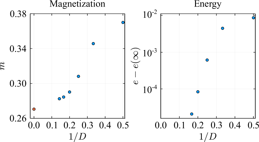
Figure 3: Results of the variational calculations with iPEPS for the antiferromagnetic Heisenberg model. The energy is plotted with respect to the extrapolated $\xi\to\infty$ value and demonstrates fast convergence. The staggered magnetization converges significantly slower, which is typical for the iPEPS calculations of gapless systems.

To extrapolate the results to the infinite-$D$ limit, we use the dependencies of the magnetization $m$ and the energy $e$ on the correlation length $\chi$ determined in Ref. Rader and Läuchli (2018):

$$m^{2}(\xi) =m^{2}(\infty)+\frac{a}{\xi},$$ (7)

$$e(\xi) =e(\infty)+\frac{b}{\xi^{3}}.$$ (8)

The dependence of the staggered magnetization on the correlation length $\xi$ is shown in Fig. 4. It clearly shows a linear behavior in accordance with the scaling formula (7). The linear fit yields the value of the magnetization $m(\infty)=0.2705(25)$, which can be compared to $m=0.27$ from the series expansion Oitmaa et al. (1992), $m=0.24$ from the spin-wave analysis Weihong et al. (1991), and to the (seemingly) most accurate Monte Carlo (MC) result $m_{\rm MC}=0.268\,82(3)$ Jiang (2012). The error was estimated from both the error of the least-squares fit and from partial fits with the reduced number of points. Note that the values of magnetization, obtained directly from the optimized iPEPS wave functions, are noticeably higher ($m>0.28$) that partially explains the higher error.

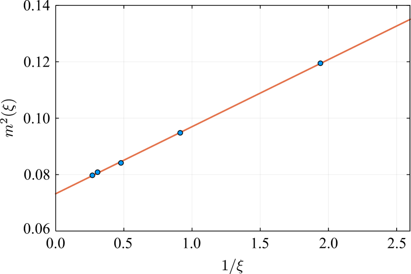
Figure 4: Dependence of the square of magnetization $m^{2}(\xi)$ for $D\in[3,7]$ on the inverse of the correlation length $\xi$ and the result of the linear fit.

In Fig. 5 we show the dependence of the energy per site $e$ on ${1}/{\xi^{3}}$ for $D\in[4,6]$, which also demonstrates a clear linear behavior in agreement with Eq. (8). At smaller $D$ (not shown in the figure), there are deviations from the ${1}/{\xi^{3}}$ dependence. For $D=6$ we obtain the energy $e=-0.544\,536$, while the energy extrapolation using the scaling formula (8) yields $e(\infty)=-0.544\,563(11)$. The quantum Monte Carlo prediction is $e_{\rm MC}=-0.544\,553(20)$ Löw (2009), hence, both the energy $e(\xi)$ for $D=6$ and the extrapolated $e(\infty)$ are within the MC error bars.

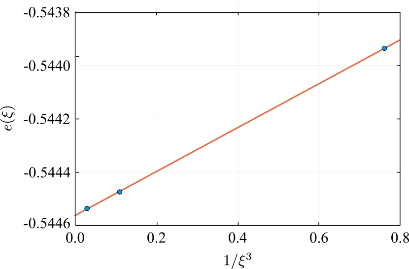
Figure 5: Dependence of the energy per site $e(\xi)$ for $D\in[4,6]$ on the the third power of the inverse of the correlation length $\frac{1}{\xi^{3}}$ and the result of the linear fit.

II.3 Kitaev model

Our CTMRG approach can not be directly applied to Hamiltonians with more general anisotropic structure of couplings, since it requires a more involved truncation procedure. We leave the development of this truncation procedure (and also the generalization to the larger unit cells) to future research. Still, there exists an important class of anisotropic Hamiltonians, which can be directly simulated with the generalization of our method. These are Hamiltonians of the Kitaev model and the corresponding generalizations known as the Kitaev-Heisenberg and $K$-$\Gamma$ models. The ferromagnetic Kitaev model has the following Hamiltonian,

$$H=-J\sum_{x_{b},ij}S^{x}_{i}S^{x}_{j}-J\sum_{y_{b},ij}S^{y}_{i}S^{y}_{j}-J\sum_{z_{b},ij}S^{z}_{i}S^{z}_{j},$$ (9)

where the sums are taken over certain types of bonds $r_{b}=\{x_{b},y_{b},z_{b}\}$ on the lattice (see also Fig. 6(b)). We hereafter fix $J=1$. The model is exactly solvable by the fermionization procedure Kitaev (2006). Its ground state at these values of parameters is a gapless spin liquid with the vanishing magnetization and the integral of motion $W=1$, which is schematically shown in Fig. 6(b).

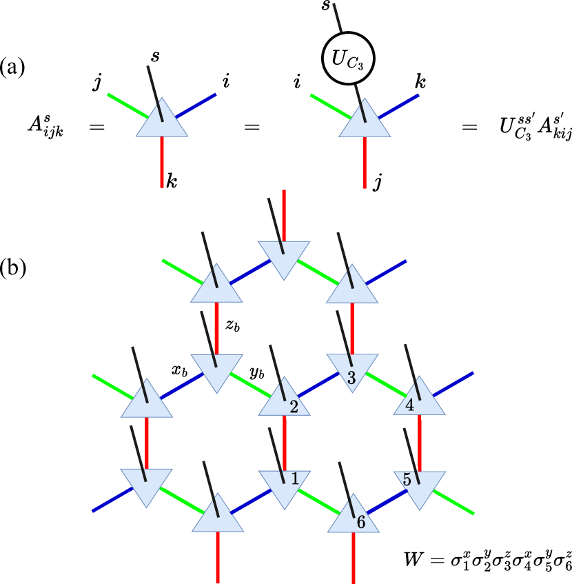
Figure 6: (a) The symmetry properties of the tensor $A$ representing the iPEPS wave function in the Kitaev model. (b) Spatial arrangement of the bonds $x_{b}$, $y_{b}$, and $z_{b}$ in the Kitaev model and the definition of the flux $W$.

From the Hamiltonian (9) it is clear that the model is not invariant under regular rotations and reflections. However, it remains invariant under transformations that belong to the modified symmetry group consisting of rotations and reflections followed by the unitary transformations on the physical Hilbert space $U_{C_{3}}R$ and $U_{p,i}p_{i}$, where $R$ is the lattice rotation, and $p_{i}$ is the lattice reflection with respect to the axis $i$. $U_{C_{3}}$ and $U_{p,i}$ are the unitary matrices, which act on the physical Hilbert space in the way to complete lattice rotations and reflections into the model symmetries. These matrices are defined as

$$U_{C_{3}}=-\exp{\left[i\frac{2\pi}{3}\right]}(I+i\sigma_{x}+i\sigma_{y}+i\sigma_{z})/2,$$ (10)

$$U_{p,z}=-(\sigma_{x}-\sigma_{y})/\sqrt{2},$$ (11)

where $I$ and $\sigma_{i}$ are the standard $2\times 2$ identity and Pauli matrices, respectively. The matrices $U_{p,y}=-\exp{\left[i\frac{2\pi}{3}\right]}(\sigma_{z}-\sigma_{x})/\sqrt{2}$ and $U_{p,x}=-\exp{\left[-i\frac{2\pi}{3}\right]}(\sigma_{y}-\sigma_{z})/\sqrt{2}$ are defined analogously. The model is additionally invariant under the time reversal, $\tau=i\sigma_{y}K$, where $K$ is the complex conjugation. It is then natural to require the iPEPS tensor $A$ to be invariant under the modified $C_{v3}$ symmetry consisting of the simultaneous rotation with the unitary transformation and reflection-conjugation modified to sequential application of the modified reflection and time reversal $\tau$. This rotation and rotation-conjugation symmetry fixes the magnetization of iPEPS to be oriented along the direction $(1,1,1)$ in the spin space. Note that tensors with the same symmetry properties were also used in Ref. Lee et al. (2019). The symmetric tensor can be obtained by the application of a projector $P$ of the form $P=I+U_{C_{3}}R+U^{2}_{C_{3}}R^{2}+i\sigma^{y}K(U_{p,x}p_{x}+U_{p,y}p_{y}+U_{p,z}p_{z})$ on the initially arbitrary iPEPS tensor $A^{s}_{ijk}$, where $U_{C_{3}}RA^{s}_{ijk}=U_{C_{3}}^{ss^{\prime}}A^{s^{\prime}}_{kij}$ and $U_{p,x}p_{x}A^{s}_{ijk}=U_{p,x}^{ss^{\prime}}A^{s}_{ikj}$. The action of this symmetry transformation is shown in Fig. 6(a).

Next, we should mention the following property of the double-layer tensor $T=\sum_{s}A^{s}_{ijk}A^{\dagger,s}_{i^{\prime}j^{\prime}k^{\prime}}$, which enters the CTM transform: It is invariant under rotations and reflection-conjugations due to cancellation of the unitary matrices $U_{C_{3}}$ and $U_{\sigma,i}$ in the double-layer contraction, thus one can apply the above-specified CTMRG approach to the given iPEPS ansatz, even if the iPEPS tensors $A$ are not rotationally invariant and the model Hamiltonian is anisotropic.

The ground-state energy of the Kitaev model (9) is determined with the exact diagonalization in the original paper Kitaev (2006), where the energy per site is equal to $e_{0}=-0.196\,82$. Our results for the energy per site for different values of the bond dimension $D$ are shown in Fig. 7. In particular, at $D=6$ the energy per site is equal to $e=-0.196\,807$. Other observables are also comparable to the exact diagonalization predictions: For $D\geq 4$ the magnetization $m<3\times 10^{-4}$ and $|1-W|<1.5\times 10^{-4}$. The correlation length $\xi$ becomes extremely large, in particular, $\xi=368$ at $D=4$, meaning that the iPEPS wave function is nearly critical. Note that our results at $D=4$ are only marginally better than the ones from Ref. Lee et al. (2019), which confirms the efficiency of their loop gas ansatz.

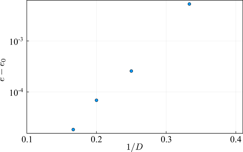
Figure 7: Dependence of the energy per site $e$ of the Kitaev model on the inverse of the bond dimension $D$. The energy is plotted with respect to the exact value $e_{0}=-0.196\,82$.

For more general anisotropic Hamiltonians, it is typically impossible to use the iPEPS ansatz with the rotationally invariant two-layer tensor $T$. Therefore, a more general CTMRG scheme must be introduced for the anisotropic tensor $T$, which should include several corner matrices $C$ for different directions and a new iteration procedure. The same procedure should be introduced to deal with the enlarged unit cells. It looks promising to develop the modified CTMRG scheme for these cases along the lines of Ref. Corboz et al. (2010).

III Conclusion and Outlook

In this paper we have realized the iPEPS variational optimization within the automatic differentiation of the honeycomb-lattice corner transfer matrix renormalization group. We tested the method on the corresponding antiferromagnetic Heisenberg and ferromagnetic Kitaev models and obtained the results comparable to the ones from the state-of-the-art quantum Monte Carlo simulations and the exact diagonalization approach.

This work opens several future research directions. The algorithm can be naturally applied to the frustrated Heisenberg antiferromagnets with NNN and even longer-range interactions Albuquerque et al. (2011); Zhang and Lamas (2013); Bishop et al. (2015); Ganesh et al. (2013); Gong et al. (2015); Ferrari et al. (2017); Gong et al. (2013). Upon certain technical modifications, it can also be employed for the star lattice geometry Jahromi and Orús (2018). Furthermore, it would be interesting to generalize the method to larger unit cells Baxter (1999). Another possible research direction is the application of the variational iPEPS to hyperbolic lattice geometries Daniška and Gendiar (2015, 2016), which were recently realized in experiments Kollár et al. (2019); Boettcher et al. (2020).

Finally, the automatic differentiation can be effectively applied to TRG and its modifications Liao et al. (2019); Chen et al. (2020). This opens a way for the variational optimization of iPEPS with the tensor renormalization.