Rooting the EDF method into the ab initio framework

Abstract

Recently, ab initio techniques have been successfully connected to the traditional valence-space shell model. In doing so, they can either explicitly provide ab initio shell-model effective Hamiltonians or constrain the construction of empirical ones. In the present work, the possibility to follow a similar path for the nuclear energy density functional (EDF) method is analyzed. For this connection to be actualized, two theoretical techniques are instrumental: the recently proposed ab initio PGCM-PT many-body formalism and the MR-IMSRG pre-processing of the nuclear Hamiltonian. Based on both formal arguments and numerical results, possible new lines of research are briefly discussed, namely to compute ab initio EDF effective Hamiltonians at low computational cost, to constrain empirical ones or to produce them directly via an effective field theory that remains to be invented.

1 Introduction

As of today, the main benefit of ab initio calculations is to rely on a systematic approach to both the input Hamiltonian and the solutions of Schrödinger’s equation in the full A-body Hilbert space ${\cal H}_{\text{A}}$ Hergert20 . This feature provides a way to improve the calculation step by step and to deliver associated uncertainties along the way. In recent years, ab initio calculations have managed to enter the domain of mid-mass nuclei thanks to approximation schemes whose numerical cost scales polynomially with the system size Hagen14 ; Hergert16 ; Soma20b ; Tichai20 . Still, the high polynomial cost currently limits the target accuracy to a few $\%$ and/or the target nucleus to mass $\text{A}\lesssim 130$.

In contrast, the main benefit of the energy density functional (EDF) method relates to a low polynomial cost associated with an a priori restriction of the explicit nucleon dynamics to a small subspace of ${\cal H}_{\text{A}}$ Bender03 ; 10.1088/2053-2563/aae0ed . This scheme makes large-scale calculations over the entire nuclear chart possible on a short time scale. However, the reduction to a subspace of ${\cal H}_{\text{A}}$ has been accompanied so far by an empirical formulation of the effective Hamiltonian at play. The current ad hoc character of the EDF method thus makes impossible to systematically test and improve associated predictions.

In this context, a legitimate objective is to build an EDF in a top-down manner, by rooting the EDF method into the ab initio theoretical scheme (for previous works of various flavours towards this objective see, e.g., Refs. Duguet15 ; Grasso16 ; Salvioni20 ; Marino21 ). The long-term objective is to make the EDF method systematic in the sense described above while maintaining its key characteristic, i.e. the low numerical cost authorizing routine calculations over the nuclear mass table. In order to achieve this goal, one must have at hand

1. an ab initio many-body method whose formulation allows an explicit connection to the subspace reduction at play in the EDF method,

2. an explicit formulation of the ab initio effective, nucleus-dependent, Hamiltonian at play in that subspace,

3. a way to systematically build that effective, nucleus-dependent, Hamiltonian without actually paying the full price of its explicit ab initio construction for each system under study.

The goal of the present paper is to demonstrate, both formally and numerically, that requirements 1. and 2. above are indeed fulfilled today. This important observation opens up a research program whose goal will be to realize point 3.

The paper is organized as follows. While Sec. 2 briefly introduces the main characteristics of ab initio and EDF theoretical schemes, Sec. 3 proceeds to a numerical comparison in ²⁰Ne, i.e. in a non-trivial doubly open-shell system. Because of the apparent irreconcilable character of ab initio and EDF results, Sec. 4 adds the key layer to the discussion constituted by the pre-processing of the Hamiltonian that, as demonstrated numerically, constitutes the missing link to reconcile the two theoretical schemes. Based on this analysis, several ideas to design a systematic EDF method in the future are briefly elaborated on in Sec. 5.

2 Formal connection

The goal of quantum many-body methods is to deliver many-body observables through a relevant theoretical scheme based on (i) an appropriate choice of degrees of freedom, (ii) a formulation of their elementary interactions and (iii) the resolution of the appropriate dynamical equation delivering the observables of interest out of these degrees of freedom and interactions.

2.1 Ab initio PGCM-PT many-body formalism

2.1.1 Theoretical scheme

The so-called ab initio description of nuclear systems is nothing but the implementation of the pion-full (or pion-less) effective field theory (EFT) in the A-nucleon sector Epelbaum:2008ga ; Machleidt:2020vzm ; vanKolck:2020plz ; vanKolck:2020llt . Taking chiral EFT ($\chi$EFT) as an example, the theoretical scheme corresponds to describing a nuclear system as a collection of (i) A non-relativistic point-like nucleons (ii) interacting via the exchange of pions and short-range contact operators in all possible ways allowed by the symmetries of QCD. In Weinberg’s power counting, observables are obtained (iii) by solving the non-relativistic A-body Schrödinger’s equation based on the Hamiltonian $H$ generated in step (ii) at a given order in the $\chi$EFT expansion, i.e.

$$H|\Psi^{\sigma}_{\mu}\rangle =E^{\tilde{\sigma}}_{\mu}\,|\Psi^{\sigma}_{\mu}\rangle\,.$$ (1)

Here $\mu$ denotes a principal quantum number whereas $\sigma\equiv(\text{J}\text{M}\Pi\text{N}\text{Z})\equiv(\tilde{\sigma}\text{M})$ collects the set of symmetry quantum numbers labelling the many-body states, i.e. the angular momentum J and its projection M, the parity $\Pi=\pm 1$ as well as neutron N and proton Z numbers (A=N+Z). The $M$-independence of the eigenenergies $E^{\tilde{\sigma}}_{\mu}$ and the symmetry quantum numbers carried by the eigenstates are a testimony of the symmetry group

$$\text{G}_{H}\equiv\{R(\theta),\theta\in D_{\text{G}}\}$$ (2)

of the Hamiltonian, i.e.,

$$[H,R(\theta)]=0\,,\,\forall\theta\,,$$ (3)

which plays a key role in the present context Frosini:2021fjf .

2.1.2 Nuclear Hamiltonian

Built at an order in the $\chi$EFT expansion where, e.g., four- and higher-body interactions vanish, the second-quantized nuclear Hamiltonian reads in an arbitrary basis of the one-body Hilbert space ${\cal H}_{1}$ as

$$H\equiv \,\,T+V+W$$

$$\equiv \,\,\frac{1}{(1!)^{2}}\sum_{\begin{subarray}{c}a_{1}\\ b_{1}\end{subarray}}t^{a_{1}}_{b_{1}}\,A^{a_{1}}_{b_{1}}$$

$$\,\,+\frac{1}{(2!)^{2}}\sum_{\begin{subarray}{c}a_{1}a_{2}\\ b_{1}b_{2}\end{subarray}}v^{a_{1}a_{2}}_{b_{1}b_{2}}\,A^{a_{1}a_{2}}_{b_{1}b_{2}}$$

$$\,\,+\frac{1}{(3!)^{2}}\sum_{\begin{subarray}{c}a_{1}a_{2}a_{3}\\ b_{1}b_{2}b_{3}\end{subarray}}w^{a_{1}a_{2}a_{3}}_{b_{1}b_{2}b_{3}}\,A^{a_{1}a_{2}a_{3}}_{b_{1}b_{2}b_{3}}\,.$$ (4)

In Eq. 4

$$A^{a_{1}\cdots a_{n}}_{b_{1}\cdots b_{n}}\equiv c^{\dagger}_{a_{1}}\cdots c^{\dagger}_{a_{n}}c_{b_{n}}\cdots c_{b_{1}}$$ (5)

denotes a string of $n$ one-particle creation and $n$ one-particle annihilation operators. While $t^{a_{1}}_{b_{1}}$ defines matrix elements of the kinetic energy, $v^{a_{1}a_{2}}_{b_{1}b_{2}}$ and $w^{a_{1}a_{2}a_{3}}_{b_{1}b_{2}b_{3}}$ characterize anti-symmetrized matrix elements of two- and three-body interactions, respectively. The nuclear Hamiltonian is thus effectively defined through a set of mode-$2k$ tensors associated with each $k$-body operator involved, the set being limited to $k\leq 3$ in the above example.

2.1.3 VSRG pre-processing

An important aspect of the present discussion regards the possibility to pre-process the Hamiltonian via unitary similarity renormalization group (SRG) transformations. For now, the nucleus-independent pre-processing based on a vacuum SRG (VSRG) transformation $U(\lambda)$ is considered in order to decouple a low-energy subspace from higher momentum modes Bogner:2009bt ; PhysRevLett.107.072501 ; PhysRevC.90.024325 . Starting from $H$ in Eq. (4), the transformed Hamiltonian reads as

$$H(\lambda)\equiv \,\,U(\lambda)HU^{\dagger}(\lambda)$$

$$\equiv \,\,T+V(\lambda)+W(\lambda)+\ldots$$

$$\equiv \,\,\frac{1}{(1!)^{2}}\sum_{\begin{subarray}{c}a_{1}\\ b_{1}\end{subarray}}t^{a_{1}}_{b_{1}}\,A^{a_{1}}_{b_{1}}$$

$$\,\,+\frac{1}{(2!)^{2}}\sum_{\begin{subarray}{c}a_{1}a_{2}\\ b_{1}b_{2}\end{subarray}}v^{a_{1}a_{2}}_{b_{1}b_{2}}(\lambda)\,A^{a_{1}a_{2}}_{b_{1}b_{2}}$$

$$\,\,+\frac{1}{(3!)^{2}}\sum_{\begin{subarray}{c}a_{1}a_{2}a_{3}\\ b_{1}b_{2}b_{3}\end{subarray}}w^{a_{1}a_{2}a_{3}}_{b_{1}b_{2}b_{3}}(\lambda)\,A^{a_{1}a_{2}a_{3}}_{b_{1}b_{2}b_{3}}$$

$$\,\,+\ldots\,,$$ (6)

such that $k$-body operators with $k>3$ are induced by the transformation. Correspondingly, the tensors defining $H(\lambda)$ acquire an explicit dependence on the parameter $\lambda$ parametrizing the transformation. The benefit of the pre-processing is to accelerate the convergence of the subsequent solving of Eq. (1) Bogner:2009bt ; PhysRevLett.107.072501 ; PhysRevC.90.024325 . This advantage must not be overtaken by more significant drawbacks, i.e. the VSRG transformation is to be stopped before induced four- and higher-body operators become too large. As a result, these induced operators are eventually discarded such that the end Hamiltonian retains the same formal expression and rank as the original $H$ in Eq. (4). For simplicity, the $\lambda$-dependence of the end result $H(\lambda)$ is omitted below.

2.1.4 Rank-reduction of the Hamiltonian

The computational cost of ab initio nuclear structure calculations is rendered particularly acute by three-nucleon interactions. Consequently, ab initio calculations of mid-mass nuclei are (currently) performed while approximating three-nucleon operators in $H$ in terms of effective, i.e. system-dependent, zero-, one- and two-nucleon operators. This is achieved in doubly closed-shell nuclei via the normal-ordered two-body approximation procedure RoBi12 whereas the rank-reduction generalization technique proposed recently in Ref. Frosini:2021tuj allows one to do so in both closed and open-shell nuclei at low computational cost. Starting from a Hamiltonian pre-processed via VSRG transformations, these approximations induce errors below $2-3\%$ across a large range of nuclei, observables and many-body methods.

In this context, the VSRG-transformed Hamiltonian $H$ is approximated by the nucleus-dependent Hamiltonian

$$\bar{H}[\rho]\equiv \,\,{\bar{h}}^{(0)}[\rho]+{\bar{h}}^{(1)}[\rho]+{\bar{h}}^{(2)}[\rho]$$

$$\equiv \,\,{\bar{h}}^{(0)}[\rho]$$

$$\,\,+\frac{1}{(1!)^{2}}\sum_{\begin{subarray}{c}a_{1}\\ b_{1}\end{subarray}}{\bar{h}}^{a_{1}}_{b_{1}}[\rho]\,A^{a_{1}}_{b_{1}}$$

$$\,\,+\frac{1}{(2!)^{2}}\sum_{\begin{subarray}{c}a_{1}a_{2}\\ b_{1}b_{2}\end{subarray}}{\bar{h}}^{a_{1}a_{2}}_{b_{1}b_{2}}[\rho]\,A^{a_{1}a_{2}}_{b_{1}b_{2}}\,,$$ (7)

where the maximum-rank has been reduced to $k=2$ and where the pure number ${\bar{h}}^{(0)}[\rho]$ has now appeared Frosini:2021tuj .

The set of mode-$2k$ tensors ($k\leq 2$) defining $\bar{H}[\rho]$ depend on the system through the symmetry-invariant one-body density matrix $\rho$ of an auxiliary symmetry-conserving many-body state. Interestingly, there exists a large flexibility regarding the nature of that auxiliary state that can typically be different from the actual solution of the Schrödinger’s equation associated to $H$ (or $\bar{H}[\rho]$) one is looking for or from the reference state employed to expand it Frosini:2021tuj . Using the density matrix extracted from a simple spherical Hartree-Fock-Bogoliubov calculation provides a good enough accuracy in practice. For simplicity, the functional dependence of $\bar{H}[\rho]$ on $\rho$ is omitted below. Of course, if the rank-reduction approximation can be avoided, $\bar{H}$ must be replaced by $H$ everywhere below.

2.1.5 PGCM-PT expansion method

The recent stepping of ab initio calculations into the realm of mid-mass nuclei has essentially been due to the development and implementation of so-called expansion many-body methods Hergert20 ; Tichai20 ; Frosini:2021fjf . Generically, these methods rely on a partitioning of the Hamiltonian

$$\bar{H} =\bar{H}_{0}+\bar{H}_{1}\,$$ (8)

chosen such that (at least) one appropriate eigenstate $|\Theta^{\sigma}_{\mu}\rangle$ of $\bar{H}_{0}$ is known, i.e.

$$\bar{H}_{0}|\Theta^{\sigma}_{\mu}\rangle =E^{\tilde{\sigma}(0)}_{\mu}\,|\Theta^{\sigma}_{\mu}\rangle\,.$$ (9)

The above partitioning of $\bar{H}$ materializes into the introduction of two projectors in direct sum on ${\cal H}_{\text{A}}$

$${\cal P}^{\tilde{\sigma}}_{\mu} \equiv\sum_{K}|\Theta^{\tilde{\sigma}K}_{\mu}\rangle\langle\Theta^{\tilde{\sigma}K}_{\mu}|\,,$$ (10a)

$${\cal Q}^{\tilde{\sigma}}_{\mu} \equiv 1-{\cal P}^{\tilde{\sigma}}_{\mu}\,.$$ (10b)

The operator ${\cal P}^{\tilde{\sigma}}_{\mu}$ projects on the eigen subspace of $\bar{H}_{0}$ spanned by the unperturbed state $|\Theta^{\sigma}_{\mu}\rangle$ along with the degenerate states obtained via symmetry transformations, i.e. belonging to the same irreducible representation (IRREP) of the symmetry group of $\bar{H}$. This constitutes the so-called ${\cal P}$ space. The operator ${\cal Q}^{\tilde{\sigma}}_{\mu}$ projects onto the complementary orthogonal subspace, the so-called ${\cal Q}$ space.

Given the unperturbed state, expansion methods aim at finding an efficient way to connect it to a target eigenstate $|\Psi^{\sigma}_{\mu}\rangle$ of $\bar{H}$. This connection is formally achieved via the so-called wave operator $\Omega$, i.e.

$$|\Psi^{\sigma}_{\mu}\rangle \equiv\Omega|\Theta^{\sigma}_{\mu}\rangle\,,$$ (11)

which is state specific and carries the complete effect of the residual interaction $\bar{H}_{1}$ in ${\cal Q}$.

In order to access all, i.e. doubly closed-shell, singly open-shell and doubly open-shell, nuclei in a controlled and polynomial fashion, the expansion method must rely on an unperturbed state $|\Theta^{\sigma}_{\mu}\rangle$ that (a) overcomes the potential occurrence of (near) degenerate elementary excitations, (b) carries good symmetry quantum numbers and (c) solves Eq. (9) at low numerical cost. While the last point imposes strong constraints on the affordable complexity of the unperturbed state, items (a) and (b) push in the opposite direction. Indeed, the first two points require that so-called strong/static correlations arising in open-shell nuclei are already incorporated into the unperturbed state in order for the subsequent expansion to be well defined and limited to capturing gentler weak/dynamical correlations.

Recently, this tension could be resolved via the formulation Frosini:2021fjf and the implementation Frosini:2021ddm of a novel expansion method coined as the projected generator coordinate method perturbation theory (PGCM-PT). The PGCM-PT formalism designs a perturbative expansion around a multi-reference symmetry-invariant unperturbed state obtained through the PGCM and thus reading as

$$|\mathrm{\Theta}^{\sigma}_{\mu}\rangle =\sum_{q}f^{\tilde{\sigma}}_{\mu}(q)P^{\tilde{\sigma}}_{M0}|\Phi(q)\rangle\,.$$ (12)

In Eq. (12), $\text{B}_{q}\equiv\{|\Phi(q)\rangle;q\in\text{set}\}$ denotes a set of non-orthogonal Bogoliubov product states differing by the value of the collective deformation parameter $q$. These reference states are typically obtained in a first step by repeatedly solving Hartree-Fock-Boboliubov (HFB) mean-field equations with a Lagrange term associated with a constraining operator $Q$ such that the solution satisfies

$$\langle\Phi(q)|Q|\Phi(q)\rangle =q\,.$$ (13)

The operator $Q$ is typically chosen such that $|\Phi(q)\rangle$ breaks symmetry(ies) of the Hamiltonian as soon as $q\neq 0$. Because physical states must carry good symmetry quantum numbers $(\tilde{\sigma},M)$, the projector $P^{\tilde{\sigma}}_{M0}$ ensures that it is the case of $|\mathrm{\Theta}^{\sigma}_{\mu}\rangle$; see Ref. Frosini:2021fjf for details regarding the symmetry group and the symmetry projector at play.

The unknown coefficients $\{f^{\tilde{\sigma}}_{\mu}(q);q\in\text{set}\}$ entering $|\mathrm{\Theta}^{\sigma}_{\mu}\rangle$ are determined via the application of Ritz’ variational principle within the PGCM subspace ${\cal H}^{\text{PGCM}}_{\text{A}}$. The latter is spanned by the set $\text{PB}_{q\tilde{\sigma}}\equiv\{P^{\tilde{\sigma}}_{M0}|\Phi(q)\rangle;q\in\text{set}\}$ of non-orthogonal projected HFB states. This leads to solving Hill-Wheeler-Griffin’s equation RiSc80

$$\sum_{q}H^{\tilde{\sigma}}_{pq}\,f^{\tilde{\sigma}}_{\mu}(q) ={\cal E}^{\tilde{\sigma}}_{\mu}\sum_{q}N^{\tilde{\sigma}}_{pq}\,f^{\tilde{\sigma}}_{\mu}(q)\,,$$ (14)

which actually delivers a set of PGCM states with associated PGCM energies

$${\cal E}^{\tilde{\sigma}}_{\mu} =\frac{\langle\Theta^{\sigma}_{\mu}|\bar{H}|\Theta^{\sigma}_{\mu}\rangle}{\langle\Theta^{\sigma}_{\mu}|\Theta^{\sigma}_{\mu}\rangle}\,.$$ (15)

Each PGCM state coming out of Eq. 14 can play the role of the unperturbed state for a target eigenstate to be reached according to Eq. 11.

The PGCM ansatz is characterized by its capacity to efficiently capture strong static correlations at play in open-shell nuclei from a low-dimensional, i.e. from several tens to a few hundreds, configuration mixing at the price of dealing with non-orthogonal vectors in the computation of the Hamiltonian ($H^{\tilde{\sigma}}_{pq}$) and norm ($N^{\tilde{\sigma}}_{pq}$) kernels RiSc80 . Such a PGCM unperturbed state renders the method universal, i.e. automatically well-behaved for doubly closed-shell, singly open-shell and doubly open-shell nuclei. In the case of closed-shell systems only displaying weak dynamical correlations, reducing the PGCM ansatz to a single symmetry-conserving Slater determinant is safe and delivers traditional single-reference expansion methods.

Selecting one of the PGCM states coming out of Eq. 14 as the unperturbed state $|\mathrm{\Theta}^{\sigma}_{\mu}\rangle$, the associated P and Q spaces are set. Next, an appropriate ab initio method must expand and truncate the wave operator $\Omega$ to capture the remaining (i.e. dynamical) correlations originating from ${\cal Q}$ to access the target state $|\mathrm{\Psi}^{\sigma}_{\mu}\rangle$. In Ref. Frosini:2021fjf , the expansion was realized designed perturbatively, thus introducing the state-specific PGCM-PT wave operator $\Omega^{\text{PGCM-PT}}$. Truncating the expansion to second order provides the PGCM-PT(2) approximation to an exact eigenvalue of $H$ through

$$E^{\tilde{\sigma}}_{\mu} =\frac{\langle\Theta^{\sigma}_{\mu}|\bar{H}|\Psi^{\sigma}_{\mu}\rangle}{\langle\Theta^{\sigma}_{\mu}|\Psi^{\sigma}_{\mu}\rangle}$$

$$=\sum_{k=0}^{\infty}E^{\tilde{\sigma}(k)}_{\mu}$$

$$\approx{\cal E}^{\tilde{\sigma}}_{\mu}+E^{\tilde{\sigma}(2)}_{\mu},$$ (16)

where the PGCM energy [Eq. (15)] of the reference state satisfies ${\cal E}^{\tilde{\sigma}}_{\mu}=E^{\tilde{\sigma}(0)}_{\mu}+E^{\tilde{\sigma}(1)}_{\mu}$ and where the calculation of the second-order correction $E^{\tilde{\sigma}(2)}_{\mu}$ is detailed in Ref. Frosini:2021fjf .

2.2 EDF many-body formalism

2.2.1 Prolegomenon

Because the nuclear EDF formalism currently relies on an empirical formulation, it still resists a truly rigorous definition and is not systematically improvable. Several interpretations have been provided throughout the years, most of which are at best incomplete and do not often correspond to what EDF calculations actually encompass in practice. Because the goal of this work is not to dispute fallacious interpretations, the formulation below pragmatically focuses on what current EDF calculations are.

Knowing that one should always start from the most general formulation out of which more limited versions derive as particular cases, the nuclear EDF formalism is presently understood as what is traditionally denoted as the multi-reference EDF (MR-EDF) method from which the single-reference level (SR-EDF) can indeed be deduced as a particular subcase.

2.2.2 Theoretical scheme

The EDF approach 10.1088/2053-2563/aae0ed also employs (i) A non-relativistic point-like nucleons as degrees of freedom. It however postulates that the A-body dynamics of these nucleons is restricted to the PGCM subspace ${\cal H}^{\text{PGCM}}_{\text{A}}$. Thus, (ii) Schrödinger’s equation delivering many-body observables is projected onto the subspace ${\cal H}^{\text{PGCM}}_{\text{A}}$ of the A-body Hilbert space ${\cal H}_{\text{A}}$ obtained via the (anti-symmetrized) tensor product of A one-body Hilbert spaces ${\cal H}_{\text{1}}$ associated with A non-relativistic point-like nucleons. Correspondingly, the EDF method (iii) postulates the existence of an effective Hamiltonian $H_{\text{EDF}}$ that can produce, within ${\cal H}^{\text{PGCM}}_{\text{A}}$, the same low-energy observables as the ab initio scheme formulated in ${\cal H}_{\text{A}}$, e.g. low-lying A-body eigenenergies can in principle satisfy

$$E^{\tilde{\sigma}}_{\mu} =\frac{\langle\Theta^{\sigma}_{\mu}|H_{\text{EDF}}|\Theta^{\sigma}_{\mu}\rangle}{\langle\Theta^{\sigma}_{\mu}|\Theta^{\sigma}_{\mu}\rangle}\,.$$ (17)

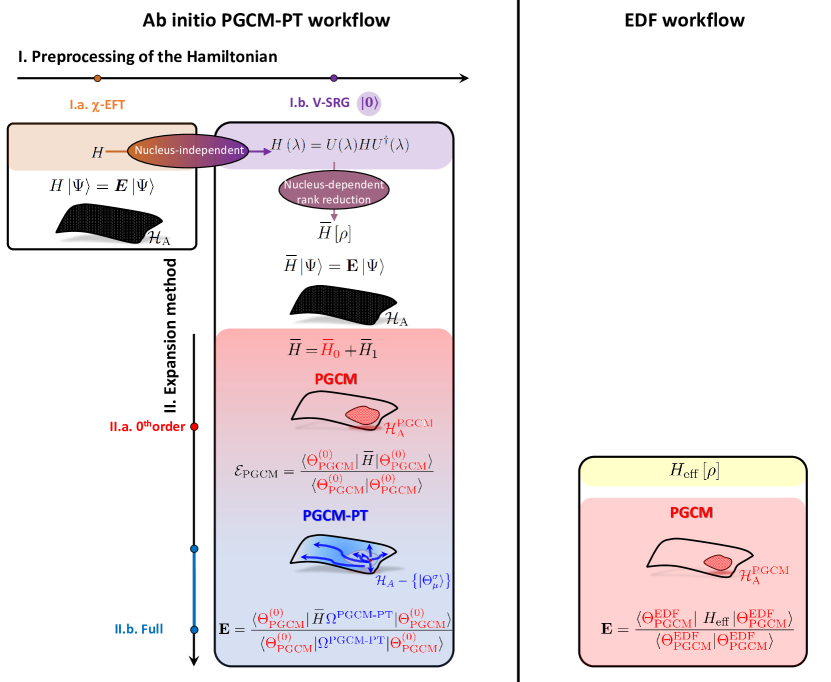
Figure 1: Schematic workflows of the two theoretical schemes. Left: the PGCM-PT ab initio many-body expansion method. Right: the (so far empirical) nuclear energy density functional many-body method.

2.2.3 Formal difficulty

Until now, the EDF method has relied on empirically-built, nucleus-dependent, effective Hamiltonians $H_{\text{EDF}}$. The nucleus dependency, crucial from the phenomenological standpoint, has been typically expressed in terms of the local one-nucleon density distribution. Originally formulated at the SR-EDF level, i.e. whenever the PGCM state reduces to a single HFB product state $|\Phi(q)\rangle$, the nucleon density was naturally computed out of this many-body state. However, the freedom left to extend this empirical ansatz to the MR-EDF case, i.e. to the PGCM ansatz, has generated intense discussions and shown to lead to problematic pathologies of various sorts depending on the choice made; see Ref. Sheikh:2019qdz and references therein for a recent summary of the issue and of the various attempts to address it.

2.3 Discussion

Before coming to a numerical comparison, let us briefly contrast the formal ingredients entering the two theoretical schemes whose workflows are schematically compared in Fig. 1.

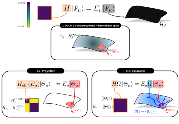
Figure 2: Many-body strategies to solve A-body Schrödinger’s equation via the PGCM partitioning of the A-body Hilbert space ${\cal H}_{\text{A}}$ into two subspaces ${\cal H}^{\text{PGCM}}_{\text{A}}$ and ${\cal H}_{\text{A}}-{\cal H}^{\text{PGCM}}_{\text{A}}$. In option 2.a., A-body Schrödinger’s equation is projected onto ${\cal H}_{\text{A}}$ to deliver the targeted eigenvalue out of an effective energy-dependent Hamiltonian. In option 2.b., the targeted eigenstate in ${\cal H}_{\text{A}}$ is expanded in terms of an eigenstate of the unperturbed Hamiltonian $\bar{H}_{0}$ belonging to ${\cal H}^{\text{PGCM}}_{\text{A}}$ and of a wave operator $\Omega$ taking explicit care of the correlations induced by the residual interaction $\bar{H}_{1}$.

For the first time, PGCM-PT provides a formally exact ab initio method whose starting point, i.e. the unperturbed state on which the many-body expansion is based, is the PGCM ansatz situated at the heart of the EDF method. According to the schematic representation displayed in Fig. 2, PGCM-PT follows strategy 2.b., i.e. while static correlations are captured within ${\cal H}^{\text{PGCM}}_{\text{A}}$, dynamical correlations are explicitly computed via the perturbative expansion of the wave operator $\Omega$ driven by $\bar{H}_{1}$.

The EDF method relies on the same partitioning of ${\cal H}_{\text{A}}$, which is eventually crucial to connect the two theoretical schemes. While static correlations are similarly captured within ${\cal H}^{\text{PGCM}}_{\text{A}}$, dynamical correlations are however now meant to be entirely compensated for via the use of $H_{\text{EDF}}$. As such, the EDF method follows, at least in principle, strategy 2.a. in Fig. 2, i.e. it proceeds through a projection on ${\cal H}^{\text{PGCM}}_{\text{A}}$. In the current empirical formulation of the EDF method, this projection is only implicit and relies on the hypothesis, never explicitly demonstrated so far, that dynamical correlations vary only smoothly with particle number and can be universally parameterized and captured through a simplistic density dependence of the effective Hamiltonian $H_{\text{EDF}}$ acting within ${\cal H}^{\text{PGCM}}_{\text{A}}$.

The specific parametrization of $H_{\text{EDF}}$, and/or of the EDF energy $E^{\tilde{\sigma}}_{\mu}$, in terms of the one-body (local) density has become the central point of discussion in the last twenty years due to the (dubious) temptation to root the nuclear EDF method into the Hohenberg-Kohn theorem of electronic density functional theory (DFT). While it might eventually be the most practical way to parameterize the nucleus dependency of $H_{\text{EDF}}$, the formulation in terms of the nucleon density distribution is not the most crucial characteristic of the EDF method (or its successor of present interest). Eventually, the key promise of the EDF method is to access essentially exact results at the low numerical cost associated with the restriction of the A-body dynamics to the PGCM subspace of ${\cal H}_{\text{A}}$ and authorize repeated calculations over the entire nuclear chart, i.e. of thousands of nuclei, on a short time scale.

Method	HFB	PGCM	PGCM-PT(2)	FCI
Runtime	$O(n_{\text{dim}}^{4})$	$O(n_{\text{proj}}n_{\text{gcm}}^{2}n_{\text{dim}}^{4})$	$O(n_{\text{proj}}n_{\text{gcm}}^{2}n_{\text{dim}}^{8})$	$O(n_{\text{dim}}^{\text{A}})$
Storage	$O(n_{\text{dim}}^{4})$	$O(n_{\text{dim}}^{4})$	$O(n_{\text{gcm}}^{2}n_{\text{dim}}^{8})$	$O(n_{\text{dim}}^{\text{A}})$

Table 1: Runtime complexity and storage requirements for various resolution methods of the many-body problem. While $n_{\text{dim}}$ denotes the dimension of the (truncated) one-body Hilbert space ${\cal H}_{\text{1}}$, $n_{\text{proj}}$ represents the number of angles used to discretize the symmetry projector $P^{\tilde{\sigma}}_{M0}$ and $n_{\text{gcm}}$ the number of states used in the mixing over $q$.

Table 1 provides the naive numerical scaling of the two theoretical schemes as a function of the basis size dimension $n_{\text{dim}}$ of the (truncated) one-body Hilbert space ${\cal H}_{\text{1}}$, which constitutes the main variable driving that scaling. While the exact solution, i.e. full configuration interaction (FCI), faces the exponential scaling of ${\cal H}_{\text{A}}$, PGCM-PT(2) displays a polynomial cost dominated by the second-order correction that scales as $n_{\text{dim}}^{8}$. Contrarily, the PGCM step, which constitutes the full cost of the EDF method, displays a much milder $n_{\text{dim}}^{4}$ scaling. Bypassing the explicit resummation of dynamical correlations and its associated computational cost is what makes the EDF method appealing. The possibility to limit many-body calculations to the EDF scaling in a controlled fashion, i.e. in a way that is rooted into the ab initio paradigm, is at the heart of the discussion below.

3 Numerical comparison

Having established a formal connection between the two theoretical schemes, the objective is now to compare the associated results for an illustrative example, i.e. the ground-state binding energy and rotational band of the doubly open-shell ²⁰Ne nucleus, and draw some useful conclusions.

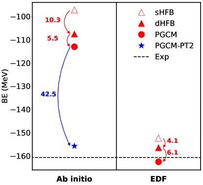
Figure 3: (color online) Successive contributions to the absolute ($J^{\pi}=0^{+}$) ground-state energy of ²⁰Ne obtained from (left) PGCM-PT(2) and (right) EDF calculations. See text for details.

The PGCM-PT calculation employs a VSRG-evolved chiral N³LO nucleon-nucleon interaction with $\lambda_{\text{vsrg}}=1.8\text{ fm}^{-1}$, supplemented with an N²LO three-nucleon interaction with cutoff $\Lambda=2.0\,\mathrm{fm}^{-1}$ whose low-energy constants are adjusted to $A=3,4$ observables, as described in Refs. PhysRevC.83.031301 ; Nogga:2004il . The Hamiltonian $H$ is turned into an in-medium two-body operator $\bar{H}[\rho]$ via the rank reduction method Frosini:2021tuj discussed in Sec. 2.1.4. The EDF calculation utilizes the relativistic point coupling parametrization DD-PC1 PhysRevC.78.034318 . Both calculations employ a spherical harmonic oscillator (HO) one-body basis characterized by the parameter $\hbar\omega=20\mathrm{\,MeV}$ and $e_{\mathrm{max}}=6$. In both cases, the PGCM state at play mixes axially-deformed HFB states constrained to the axial quadrupole moment ($q\equiv q_{20}$) $\beta_{2}\in[0.3,0.8]$ and further projected on good neutron $N$ and proton $Z$ numbers as well as on good total angular momentum $J$.

Figure 3 displays the successive contributions to ²⁰Ne ground-state energy, i.e. (a) spherical HFB (sHFB), (b) deformed HFB (dHFB), (c) PGCM and, for the ab initio calculation, adding the (d) PGCM-PT(2) correction. The striking observation is that the energies generated through the first three steps are very different in the two calculations. While the PGCM step is final in the EDF calculation, and thus close to the experimental value, the corresponding ab initio result is about 45 MeV unbound. Thankfully, this deficit is consistently compensated for by the explicit inclusion of dynamical correlations via the second-order PGCM-PT(2) correction. While both calculations are eventually satisfactory, they reach the end result in an apparently very different fashion in spite of employing the same technique to grasp static correlations via the PGCM.

This apparent mismatch and the key role played by explicit dynamical correlations in the ab initio calculation seem to forbid a practical connection between the two theoretical schemes. Under closer inspection, one observes that the scales at play in steps (b) (sHFB$\longrightarrow$dHFB) and (c) (dHFB$\longrightarrow$PGCM) taking care of static correlations are, if not identical, actually consistent in both calculations. Eventually, the difference mostly correlates with a shift up of the ab initio starting point (sHFB) that is essentially compensated for by the PGCM-PT(2) correction. This examination indicates that there might be a way to relate the two schemes in a more transparent and explicit fashion.

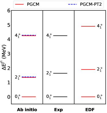
Figure 4: (color online) Low-lying part of ²⁰Ne ground-state rotational band. Left: PGCM-PT(2) calculation. Middle: experimental data. Right: EDF calculation. See text for details.

Before coming to this key point, the analysis is extended to the low-lying part of ${}^{20}\mathrm{Ne}$ ground-state rotational band in Fig. 4. Quite strikingly, the ab initio PGCM spectrum is in excellent agreement with experiment. Consistently, the large PGCM-PT(2) correction ($\sim 45$ MeV) to each absolute energy cancels out to a high degree and leave the spectrum essentially unchanged, making ab initio PGCM calculations already well suited to describe low-lying rotational bands. As seen from the right panel, the EDF spectrum is slightly too spread out. While the degree of dilatation depends on the specific parameterization used and happens to be rather moderate with DD-PC1, this dilatation is a generic feature of rotational bands obtained in PGCM calculations performed within the EDF context whenever based on the sole axial quadrupole shape degree of freedom.

4 Pre-processing of the Hamiltonian

When computing total energies, as in the example displayed in Fig. 3, it is not surprising that the first three steps of ab initio and EDF calculations lead to different results. Indeed, although based on the same (i.e. PGCM) wave-function ansatzes, the two calculations differ by the very nature of the employed Hamiltonians, i.e. while $H$ is defined over ${\cal H}_{\text{A}}$, $H_{\text{EDF}}$ effectively operates in a subspace of it. Thus, the key to a consistent connection between the two theoretical schemes relies on a meaningful link between the two Hamiltonians at play. A formally transparent approach to connect the Hamiltonian $H$ acting on ${\cal H}_{\text{A}}$ to an effective Hamiltonian whose action is restricted to the subspace ${\cal H}^{\text{PGCM}}_{\text{A}}$ is provided by (non-unitary) subspace projection techniques feshbach58a ; feshbach62a . This procedure typically produces an energy- and system-dependent A-body effective Hamiltonian that delivers the same low-energy eigenvalues as $H$ while acting on the targeted subspace. In order to avoid the complexity of dealing with an energy-dependent Hamiltonian, the use of multi-reference unitary in-medium similarity renormalization group (MR-IMSRG) transformations Tsukiyama:2010rj ; Hergert16 of the initial Hamiltonian is presently advocated to effectively decouple ${\cal H}^{\text{PGCM}}_{\text{A}}$ from the complementary subspace of ${\cal H}_{\text{A}}$.

4.1 MR-IMSRG transformations

As for an actual presentation of MR-IMSRG transformation techniques, the reader is referred to Refs. Hergert16 ; Hergert:2016iju ; Hergert:2016etg . For the present purpose, it is sufficient to stipulate the existence of a continuous manifold of nucleus-dependent unitary transformations ${\cal U}(s)$ parameterized by a momentum scale $s$ and tailored such that the PGCM reference state becomes largely decoupled from the orthogonal subspace of ${\cal H}_{\text{A}}$, the ${\cal Q}$ space, via the transformed Hamiltonian $\bar{H}(s)\equiv{\cal U}(s)\bar{H}{\cal U}^{\dagger}(s)$ when $s\rightarrow\infty$.

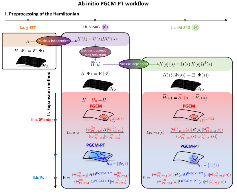
Figure 5: Extended ab initio PGCM-PT workflow including the MR-IMSRG pre-processing of the Hamiltonian.

Applying the unitary transformation to Eq. (1) formally leads to

$$\bar{H}(s)|\Psi^{\sigma}_{\mu}(s)\rangle =E^{\tilde{\sigma}}_{\mu}\,|\Psi^{\sigma}_{\mu}(s)\rangle\,,$$ (18)

with

$$|\Psi^{\sigma}_{\mu}(s)\rangle \equiv{\cal U}(s)|\Psi^{\sigma}_{\mu}\rangle$$

$$\equiv\Omega^{\text{PGCM-PT}}(s)|\Theta^{\sigma}_{\mu}(s)\rangle\,,$$ (19)

where the last line testifies that the PGCM state acquires an explicit $s$ dependence given that it is eventually re-computed from the transformed Hamiltonian $\bar{H}(s)$. As opposed to the (energy-dependent) Hamiltonian obtained via non-unitary subspace projection techniques, $\bar{H}(s)$ still acts on the complete A-body Hilbert space. However, it does so in such a way that the PGCM state becomes more and more decoupled from the orthogonal subspace as $s\rightarrow\infty$. The MR-IMSRG pre-processing of $\bar{H}$ adds one layer to the ab initio workflow as schematically illustrated in Fig. 5 where the intensity of the coupling between ${\cal P}$ and ${\cal Q}$ subspaces is reduced as $s$ increases.

While the full eigenvalue $E^{\tilde{\sigma}}_{\mu}$ remains invariant under the unitary transformation ${\cal U}(s)$ as stipulated by Eq. (18), wave-functions and intermediate contributions to the total energy all vary with $s$. In fact, Eqs. (18) and (19) indicate that correlations are shifted from the initial wave-function to the Hamiltonian through the transformation ${\cal U}(s)$ such that a reshuffling of correlations shall occur as a function of $s$ while maintaining the total energy unchanged. If the PGCM state could be entirely decoupled from the complementary subspace at the end of the flow, the identity $\Omega^{\text{PGCM-PT}}(\infty)=1$ would hold. As mentioned earlier, complete decoupling can be achieved in principle for SR-IMSRG transformations based on Slater determinant reference states, but typically not in the more general MR-IMSRG case.

The MR-IMSRG represents the Hamiltonian and other observables in a basis of second-quantized operators $:A^{a_{1}a_{2}\ldots}_{b_{1}b_{2}\ldots}:$ in normal order with respect to the correlated unperturbed state, i.e. the PGCM state $|\Theta^{\sigma}_{\mu}\rangle$ in the present case. This is done employing the generalized normal ordering and Wick’s theorem developed by Mukherjee and Kutzelnigg Kutzelnigg:1997fk and leads to

$$\bar{H}(s)\equiv \,\,{\cal U}(s)\bar{H}{\cal U}^{\dagger}(s)$$

$$\equiv \,\,{\bar{h}}^{(0)}(s)+:{\bar{h}}^{(1)}(s):+:{\bar{h}}^{(2)}(s):+\ldots$$

$$\equiv \,\,{\bar{h}}^{(0)}(s)$$

$$\,\,+\frac{1}{(1!)^{2}}\sum_{\begin{subarray}{c}a_{1}\\ b_{1}\end{subarray}}{\bar{h}}^{a_{1}}_{b_{1}}(s)\,:A^{a_{1}}_{b_{1}}:$$

$$\,\,+\frac{1}{(2!)^{2}}\sum_{\begin{subarray}{c}a_{1}a_{2}\\ b_{1}b_{2}\end{subarray}}{\bar{h}}^{a_{1}a_{2}}_{b_{1}b_{2}}(s)\,:A^{a_{1}a_{2}}_{b_{1}b_{2}}:$$

$$\,\,+\frac{1}{(3!)^{2}}\sum_{\begin{subarray}{c}a_{1}a_{2}a_{3}\\ b_{1}b_{2}b_{3}\end{subarray}}{\bar{h}}^{a_{1}a_{2}a_{3}}_{b_{1}b_{2}b_{3}}(s)\,:A^{a_{1}a_{2}a_{3}}_{b_{1}b_{2}b_{3}}:$$

$$\,\,+\ldots\,,$$ (20)

where $:\ldots:$ denotes the normal ordering with respect to $|\Theta^{\sigma}_{\mu}\rangle$. In the process, the tensors defining the evolved Hamiltonian not only acquire a dependence on $s$ as explicitly indicated in Eq. (20) but also become functionals of the set of irreducible density matrices associated with $|\Theta^{\sigma}_{\mu}\rangle$

$$\lambda^{a_{1}}_{b_{1}} \equiv\langle\Theta^{\sigma}_{\mu}|A^{a_{1}}_{b_{1}}|\Theta^{\sigma}_{\mu}\rangle\,,$$ (21a)

$$\lambda^{a_{1}a_{2}}_{b_{1}b_{2}} \equiv\langle\Theta^{\sigma}_{\mu}|A^{a_{1}a_{2}}_{b_{1}b_{2}}|\Theta^{\sigma}_{\mu}\rangle-\mathcal{A}\left(\lambda^{a_{1}}_{b_{1}}\lambda^{a_{2}}_{b_{2}}\right)\,,$$ (21b)

$$\lambda^{a_{1}a_{2}a_{3}}_{b_{1}b_{2}b_{3}} \equiv\langle\Theta^{\sigma}_{\mu}|A^{a_{1}a_{2}a_{3}}_{b_{1}b_{2}b_{3}}|\Theta^{\sigma}_{\mu}\rangle-\mathcal{A}\left(\lambda^{a_{1}}_{b_{1}}\lambda^{a_{2}}_{b_{2}}\right)$$

$$\qquad-\mathcal{A}\left(\lambda^{a_{1}a_{2}}_{b_{1}b_{2}}\lambda^{a_{3}}_{b_{3}}\lambda^{a_{3}}_{b_{3}}\right)\,,$$ (21c)

$$\vdots$$

where the antisymmetrizer $\mathcal{A}$ generates all unique index permutations of its arguments that are required to ensure overall antisymmetry; i.e.

$${\bar{h}}^{a_{1}\ldots}_{b_{1}\ldots}(s)\equiv{\bar{h}}^{a_{1}\ldots}_{b_{1}\ldots}(\{\lambda^{a_{1}\ldots}_{b_{1}\ldots}\};s)\,.$$ (22)

Using these irreducible density matrices as generalized contractions, the basis of normal-ordered operators is defined recursively as

$$:A^{a_{1}}_{b_{1}}: =A^{a_{1}}_{b_{1}}-\lambda^{a_{1}}_{b_{1}}\,,$$ (23a)

$$:A^{a_{1}a_{2}}_{b_{1}b_{2}}: =A^{a_{1}a_{2}}_{b_{1}b_{2}}-\mathcal{A}\left(\lambda^{a_{1}}_{b_{1}}\lambda^{a_{2}}_{b_{2}}\right)-\lambda^{a_{1}a_{2}}_{b_{1}b_{2}}\,,$$ (23b)

$$\vdots$$

Details can be found in, e.g., Ref. Hergert:2016etg .

In actual calculations, the total energy is not strictly independent of $s$ due to the necessary approximations made on (i) the MR-IMSRG transformation that is truncated at the MR-IMSRG(2) level, i.e. mode-$2k$ tensors with $k\geq 3$ in Eq. (20) are consistently set to $0$ all throughout the transformation, and on (ii) the PGCM-PT expansion that is truncated at the PGCM-PT(2) level. Given the necessity to compute the PGCM-PT(2) correction anyway, one can avoid pushing the MR-IMSRG transformation to very large $s$ in order to limit the breaking of unitarity occurring at the MR-IMSRG(2) level.

4.2 Numerical results

The PGCM-PT(2) calculation of ²⁰Ne is repeated for two MR-IMSRG(2) pre-processed Hamiltonians characterized by the flow parameters $s=10,20$ MeV^-1 in addition to the unprocessed one ($s=0$) discussed earlier.

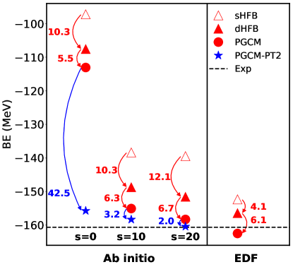
Figure 6: (color online) Same as Fig. 3 except that the ab initio calculation is performed for three values ($s=0,10,20$ MeV^-1) of the MR-IMSRG pre-processing parameter of the Hamiltonian.

The systematic effect of the MR-IMSRG pre-processing of the Hamiltonian on the absolute binding energy of ${}^{20}\mathrm{Ne}$ is shown in Fig. 6. The MR-IMSRG evolution largely reshuffles the hierarchy of correlations at play. As $s$ grows, one observes that

1. the sHFB energy is drastically lowered due to the a prori resummation of the bulk of dynamical correlations into $\bar{H}(s)$,

2. static correlations captured at the PGCM level are stable throughout the process, only slightly increasing from about $16$ MeV at $s=0$ MeV^-1 to about $19$ MeV at $s=20$ MeV^-1, remaining overall consistent with the static correlations ($10$ MeV) captured within the EDF calculation,

3. dynamical correlations explicitly grasped on top of PGCM through the PGCM-PT(2) correction are drastically reduced from being highly dominant at $s=0$ MeV^-1 ($42$ MeV) to being largely subleading at $s=20$ MeV^-1 ($2$ MeV).

The picture that emerges is that, by resumming $95\%$ of the initial dynamical correlations into the pre-processed Hamiltonian $\bar{H}(s)$, the scales and hierarchy of correlations become highly consistent with those at play in the EDF calculation. Thus, the apparent inconsistency between the results obtained from both theoretical schemes in Sec. 3 is lifted such that both a qualitative and quantitative link between them is now at reach.

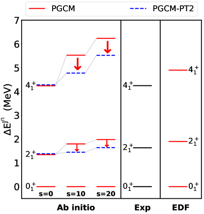
Figure 7: (color online) Same as Fig. 4 except that the ab initio calculation is performed for three values ($s=0,10,20$ MeV^-1) of the MR-IMSRG pre-processing parameter of the Hamiltonian.

The effect of the MR-IMSRG pre-processing on ²⁰Ne ground-state rotational band is displayed in Fig. 7. As already seen in Fig. 4, the ab initio PGCM spectrum is essentially perfect at $s=0$ MeV^-1 and the corresponding PGCM-PT(2) correction essentially zero. The picture changes significantly when pre-processing the Hamiltonian via MR-IMSRG. Indeed, the ab initio PGCM spectrum becomes more and more dilated as $s$ grows and resembles the EDF spectrum for $s\approx 10$ MeV^-1. Consistently, the second-order PGCM-PT(2) correction increases with $s$ and systematically corrects for the dilatation, although not sufficiently for large $s$, in particular for the $4^{+}_{1}$ state.

4.3 Discussion

The above numerical results demonstrate that the empirical nuclear EDF method can be meaningfully rooted into the ab initio theoretical scheme for two key reasons.

1. The family of MR-IMSRG pre-processed Hamiltonians $\bar{H}(s)$ is suited to play, for moderate-to-large $s$ values, the role of an effective and nucleus-dependent Hamiltonian acting within the restricted PGCM subspace ${\cal H}^{\text{PGCM}}_{\text{A}}$; i.e. the role of an ab initio version of $H_{\text{EDF}}$. Of course, using $\bar{H}(s)$ per se simply amounts to performing the ab initio calculation and to paying the computational cost of its construction in each nucleus, which does not fit the philosophy of an EDF-like scheme. As shown in Tab. 2, building $\bar{H}(s)$ at the MR-IMSRG(2) level indeed scales as $O(n_{\text{dim}}^{6})$ and thus largely dominates the cost of a PGCM calculation performed with it. Going to the MR-IMSRG(3) truncation scheme for greater accuracy further increases the scaling to $O(n_{\text{dim}}^{9})$, which is already beyond current capabilities for state-of-the-art ab initio calculations Heinz:2021xir ; Hoppe:2021xqv . In order to actually root the construction of $H_{\text{EDF}}$ into $\bar{H}(s)$, one must find ways to significantly decrease the cost to construct the latter. Possible lines of research in this direction are briefly alluded to in Sec. 5 below.

2. For moderate-to-large $s$ values, residual dynamical correlations captured via perturbation theory on top of PGCM are small. This is mandatory for a viable EDF-like scheme that wishes to effectively remain at the PGCM level and avoid altogether the need to perform, e.g., PGCM-PT(2) calculations whose cost scales as $O(n_{\text{dim}}^{8})$. Strictly speaking though, the above results show that the residual coupling between the PGCM states and the complementary subspace is not zero for $s$ values of interest and even slightly magnified for the excitation spectrum compared to $s=0$ MeV^-1. While an ab initio-rooted EDF scheme limited to a $O(n_{\text{dim}}^{4})$ numerical scaling has to tolerate a degree of inaccuracy compared to a high-level ab initio scheme, it is of interest to further limit the coupling to the ${\cal Q}$ space for both ground and excited states at once. In this way, the systematic error made by omitting that coupling would be minimized. This idea will also be elaborated on Sec. 5.

Method	MR-IMSRG(2)	MR-IMSRG(3)
Runtime	$O(n_{\text{dim}}^{6})$	$O(n_{\text{dim}}^{9})$
Storage	$O(n_{\text{dim}}^{4})$	$O(n_{\text{dim}}^{6})$

Table 2: Runtime complexity and storage requirements of the MR-IMSRG(2) and MR-IMSRG(3) pre-processing methods.

5 Perspectives

As explained above, rooting an EDF-like scheme into the ab initio PGCM-PT formalism based on MR-IMSRG Hamiltonians requires (i) to make the PT corrections on top of the PGCM essentially negligible and (ii) to reduce significantly the cost to construct $\bar{H}(s)$. Indeed, this is mandatory to build an effective theory that operates with a mean-field-like scaling ($O(n_{\text{dim}}^{4})$) independently of the nucleus under study and thus authorize a wide-spread or even universal applicability across the nuclear chart, ideally with a high level of physical interpretability.

In the following, several potential lines of research to progess towards points (i) and (ii) are briefly elaborated on.

5.1 Improving the ${\cal Q}$-space decoupling

5.1.1 Enriching the PGCM state

The function of the MR-IMSRG pre-processing is to decouple the PGCM state(s) from the rest of the Hilbert space and build the associated correlations into the evolved Hamiltonian.

In practice, the span of ${\cal H}^{\text{PGCM}}_{\text{A}}$ can impact the quality of the decoupling. This is controlled by the choice of the generator coordinates actually defining the PGCM at play. The expectation is that progressively enriching the PGCM ansatz to include relevant relevant correlations can effectively reduce its coupling to the rest of the Hilbert space.

The ${}^{20}\mathrm{Ne}$ results displayed in Figs. 3 and 6 were obtained with an ansatz based on axially and time-reversal symmetric fully paired HFB vacua. However, it was demonstrated earlier on Frosini:2021sxj that the inclusion of the octupole degree of freedom is necessary to describe the spectrum of this nucleus more quantitatively. In general, the inclusion of octupole, triaxial and/or pairing degrees of freedom is expected to be useful in a variety of doubly open-shell nuclei. Moreover, HFB states obtained via a variation after particle-number-projection calculation or via the use of a cranking constraint breaking time-reversal invariance can compress dilated PGCM spectra PhysRevLett.113.162501 ; Borrajo:PLB2015 ; Yao:2019rck ; Hergert20 and thus further suppress the residual dynamical correlations on top of the PGCM via, e.g. PGCM-PT. Last but not least, the inclusion of a few HFB states obtained via elementary excitations of fully paired HFB vacua is also expected to be useful in some specific situations Frosini:2021sxj , as a means to describe non-collective excitations. While the enrichment of the PGCM ansatz can significantly increase the CPU cost, it will remain highly subleading, especially as the nuclear mass grows, compared to the $n_{\text{dim}}^{8}$ cost associated with the explicit inclusion of dynamical correlations via PGCM-PT(2).

5.1.2 Improving the MR-IMSRG transformation

Apart from the characteristics of ${\cal H}^{\text{PGCM}}_{\text{A}}$, one may improve various characteristics of the MR-IMSRG transformation itself. While going to more advanced truncation schemes, e.g. MR-IMSRG(3), constitutes an obvious way to improve the $\mathcal{Q}$-space decoupling, it contradicts the goal to achieve the EDF-like $O(n_{\text{dim}}^{4})$ computational cost. It is thus not an option and other ideas must be envisioned.

As already alluded to, the decoupling conditions are generally more complex for MR-IMSRG than for the SR-IMSRG: terms that vanish automatically for a Slater determinant reference state are no longer zero when normal-ordering the Hamiltonian with respect to PGCM states such that additional contributions originating from two-body and higher irreducible density matrices (cf. Eq. (21)) arise. Eventually, a state or a group of states cannot be strictly decoupled from the rest of the Hilbert space. Still, approximate decoupling happens because the flow explores and eventually decouples the space of particle-hole like excitations that are built on the individual components of the correlated state Gebrerufael:2017fk ; Yao:2018wq ; Yao:2019rck . Doing so, the evolution performed with respect to the PGCM ground state usually improves all states belonging to the associated rotational band although excited states tend to gain less energy because the transformation is (implicitly) tuned for the ground state reference. This feature likely explains the spreading of the excitation spectrum of ${}^{20}\mathrm{Ne}$ in Sec. 4 and calls for an improvement.

Reference ensemble

Starting with the latter point, the normal ordering and MR-IMSRG evolution can be performed with respect to a reference ensemble rather than with respect to a pure reference state. This procedure was first introduced in valence-space IMSRG (VS-IMSRG) calculations of open-shell nuclei Stroberg:2016ung ; Stroberg:2019th to account for partially filled orbitals in the calculation of ground-state energies. However, one can also view it as a mean to optimize the decoupling of the valence space as a whole. A similar observation was made in quantum chemistry Watson:2016eu . Closer to the present problem of interest, ensembles of PGCM states were used to optimize the MR-IMSRG operator basis for the calculation of electromagnetic neutrinoless double beta decay transitions as well as the electromagnetic transitions in either nucleus Yao:2019rck ; Yao:2021bs ; Yao:2022nv . Here, an ensemble built out of the PGCM states solution of the Hill-Wheeler equation could be employed to optimize the decoupling of ${\cal H}^{\text{PGCM}}_{\text{A}}$ at once rather than of the ${\cal P}$ space defined by a single PGCM state. In this way, the entire PGCM spectrum could be improved in a single calculation, thus avoiding the spreading observed in Sec. 4.

Improved operator basis

It may be useful to see the MR-IMSRG through the lens of RG theory to tackle both accuracy and efficiency goals. The first step of any RG scheme is usually the selection of an appropriate operator basis to describe the RG flow. Importantly, the flow equations themselves can provide a diagnostic to identify relevant, marginal or irrelevant operators, and whether the initially chosen set is sufficiently complete whenever truncated or if relevant induced operators have been discarded. Furthermore, the identification and omission of irrelevant operators can immediately lead to a significant reduction of the computational effort whenever a high degree of redundancy exists in the operator basis. At the same time, the invariance of observables under MR-IMSRG evolution, or lack thereof, indicates whether the chosen operator basis is sufficiently complete and accurate.

In the present context, the normal ordering procedure itself can be viewed as a mean to optimize the basis of second-quantized operators $:A^{a_{1}\ldots}_{b_{1}\ldots}:$. As a matter of fact, going from simple reference states to suitably optimized correlated reference states, like PGCM states for open-shell nuclei, can turn some omitted operators from being relevant in SR-IMSRG(2) to being irrelevant in MR-IMSRG(2), thus reducing the truncation errors and flow-parameter dependence without altering the size of the basis. The optimal character of the operator basis can be further improved for a given reference state by exploiting the flexibility offered by the Mukherjee-Kutzelnigg scheme Kong:2010kx . First, it is possible to choose which of the irreducible density matrices are treated as contractions in Wick’s theorem and which ones are included explicitly only when the many-body matrix element of an operator is evaluated. For example, the usual set of conditions

$$\langle\Theta^{\sigma}_{\mu}|:A^{a_{1}\ldots}_{b_{1}\ldots}:|\Theta^{\sigma}_{\mu}\rangle=0\,,$$ (24)

can be replaced by

$$\langle\Theta^{\sigma}_{\mu}|:A^{a_{1}}_{b_{1}}:|\Theta^{\sigma}_{\mu}\rangle =0\,,$$ (25a)

$$\langle\Theta^{\sigma}_{\mu}|:A^{a_{1}a_{2}}_{b_{1}b_{2}}:|\Theta^{\sigma}_{\mu}\rangle =\lambda^{a_{1}a_{2}}_{b_{1}b_{2}}\,,$$ (25b)

$$\ldots{}$$

in order to adapt the definition of the normal-ordered operators at play. Indeed, there is evidence from applications in nuclear physics Hergert:2014iaa ; Hergert:2016etg and quantum chemistry Datta:2011cr ; Datta:2012zr that it is sufficient to only retain the (correlated) one-body density matrix $\lambda^{a_{1}}_{b_{1}}$ of the reference state to construct normal-ordered operators according to Eq. (25), thus making the tensors defining $\bar{H}(s)$ (Eq. (20)) functionals of the one-body density matrix alone. One must however be aware that the particular choice of generator and the “extent” of the transformation as measured by the flow parameter $s$ can affect whether the higher irreducible density matrices are indeed negligible.

Second, the only property that the irreducible density matrices must actually fulfill to apply the normal ordering formalism is their antisymmetry under permutations of the upper and lower indices Kong:2010kx . Thus, it is in fact not necessary to require that the employed density matrices are associated with the reference, e.g. PGCM, state or with any many-body state for that matter. Relaxing this constraint and limiting Wick contractions to the one-body density matrix alone, the latter can be viewed as a tunable auxiliary quantity to be optimized for any given purpose, e.g. adapt the operator basis to improve the accuracy of the flow and to minimize the residual coupling to the rest of the Hilbert space. As a proof of principle, this idea was recently exploited to minimize the violation of unitarity of the MR-IMSRG flow in a pairing plus particle-hole interaction toy model Davison:2022a . While this study relied on the ability to compute the exact eigenvalues of a complete block of $\bar{H}(s)$ in a full configuration approach, it can be adapted to realistic applications in the future. This will require the use of a cost function characterizing the unitarity of the evolution and/or the residual coupling while allowing a fast evaluation of the density matrix gradients, so that the desired $O(n_{\text{dim}}^{4})$ is maintained. Eventually, the use of an auxiliary density matrix in the construction of the operator basis could also be useful to smooth out features of particular nuclei or states and help design a “universal” EDF-like Hamiltonian $\bar{H}(s)$.

5.2 Mitigating the construction cost of $\bar{H}(s)$

One of the main reasons to pursue an approach with EDF-like $O(n_{\text{dim}}^{4})$ scaling is that will enable large-scale investigations of observables across the nuclear chart while also exploring the parameter spaces of the underlying interactions. This is key for the ongoing effort to refine our understanding of these interactions and to systematically account for associated uncertainties.

While the previous section focused on ideas to avoid the $O(n_{\text{dim}}^{8})$ cost of PGCM-PT(2) altogether, the present section looks into possibilities to reduce, or even bypass eventually, the MR-IMSRG cost associated with the construction of $\bar{H}(s)$, knowing that MR-IMSRG with explicit $k-$body operators, i.e., an MR-IMSRG(k) truncation, naively requires $O(n_{\text{dim}}^{3k})$ operations and $O(n_{\text{dim}}^{2k})$ memory.

Unsurprisingly, several efforts in the nuclear many-body community are underway to reduce these runtime and memory costs. At their heart lies the idea that these computational costs are in no small part caused by redundancies in the chosen representations of the interactions and many-body states, and that more efficient reduced-order models can be found (see Refs. Melendez:2022kid ; Bonilla:2022rph for an introduction and overview).

5.2.1 Reference ensemble

One way to alleviate the construction cost of $\bar{H}(s)$ is to improve its universal character without yet reducing the cost of a single MR-IMSRG run. Naively, the MR-IMSRG evolution, and thus the construction of $\bar{H}(s)$, is to be performed for each quantum state of each nucleus. The idea discussed in the previous section to evolve the Hamiltonian with respect to the ensemble of PGCM states rather than with respect to each PGCM state separately is already a way to go beyond that naive approach. Furthermore, observables in the two nuclei involved in the neutrinoless double beta decay were shown in Ref. Yao:2019rck ; Yao:2021bs ; Yao:2022nv to be remarkably insensitive to sizable variations in the weights of the ensemble members. This observation is promising in view of yet enlarging the ensemble of PGCM states to generate MR-IMSRG evolved Hamiltonians $\bar{H}(s)$ that could not only be optimized for various quantum states of a given nucleus but also for several nuclei at once. It remains to be shown how far such an idea can pushed, i.e. what typical range of nuclei and quantum states can be successfully addressed from a single Hamiltonian $\bar{H}(s)$.

5.2.2 Pre-processing techniques

In recent years, different techniques aiming at reducing the computational cost of many-body methods have been put forward. The goal of such techniques is to lower the computation cost $O(n_{\text{dim}}^{p})$ by (effectively) reducing either the exponent $p$ (e.g. via tensor factorization) or the dimension of the one-body Hilbert space $n_{\text{dim}}$ needed to yield converged results (e.g. via the use of importance truncation or natural orbitals). While the former is expected to yield a more decisive advantage since it targets the exponent $p$ and thus directly meets the goal to go from, e.g. $O(n_{\text{dim}}^{6})$ down to $O(n_{\text{dim}}^{4})$, the combination of both types of pre-processing tools is likely to prove crucial in the long term in order to push the limits of applicability of many-body calculations.

Tensor factorization

While (tensor) factorization techniques have been explored with great success in quantum chemistry Schutski:2017xr ; Parrish:2019zg ; Hohenstein:2022oj ; Lesiuk:2020hq , applications in nuclear physics are still in their infancy Parrish:2013fe ; Tichai:2019xz ; Tichai:2022rq . The key challenge to achieve a scaling reduction is to reformulate many-body methods like the MR-IMSRG in such a way that they directly operate with the factors out of which the tensors defining the Hamiltonian and the unknown of the problem are built. This constitutes a promising but highly nontrivial task Tichai:2022rq ; Schutski:2017xr ; Parrish:2019zg .

Importance truncation

The goal of importance truncation (IT) techniques is to discard, prior to running the full costly calculation, some of the entries of the unknown many-body tensors at play in a given method. This selection can be efficiently performed on the basis of a less expensive method, typically some variant of many-body perturbation theory. IT techniques have already been successfully applied to few many-body approaches Roth:2009eu ; TICHAI2019 ; Porro:2021rw including the single-reference IMSRG Hoppe:2021xqv .

Natural basis

Among the possible strategies to optimise the single-particle basis, a promising procedure consists in the use of the so-called natural basis. The main idea is that natural orbitals, i.e. the eigenbasis of a correlated one-body density matrix, are already informed from (dynamical) correlations at play, thus effectively reducing the size $n_{\text{dim}}$ of the one-body basis needed to explicitly incorporate those (dynamical) correlations via the high-level method of interest. As for IT, the correlated one-body density matrix out of which natural orbitals are extracted is to be computed via some inexpensive approach like second-order perturbation theory. The use of natural orbitals has been recently explored in different methods Tichai:2019to ; Hoppe:2020elo ; Fasano:2021ahd such that the extension to MR-IMSRG can be envisaged in the future.

5.2.3 Emulators

In addition to accelerating individual MR-IMSRG runs needed to build $\bar{H}(s)$, emulators can be used to reduce the cost of large sets of calculations. They exploit smooth parameter dependences of the Hamiltonian, its eigenstates and associated observables. The full calculation is performed for a selection of parameter sets in order to generate training data for the emulator, which acts as a surrogate model that can predict the results for other parameter values with high accuracy at a fraction of the computational cost.

The so-called eigenvector continuation (EC) approach constitutes a particularly successful basis for emulators of wave-function-based methods Frame:2018bv ; Demol:2020nm ; Konig:2020fn ; Ekstrom:2019tw ; Wesolowski:2021vr ; Melendez:2021sy ; Zhang:2022dk . In the present context, a potentially impactful idea would be to treat the dependence of $\bar{H}(s)$ on the auxiliary density matrix via EC, so that MR-IMSRG evolutions would not have to be performed explicitly for each nucleus and parameter sets, but only for the training data. The main challenge is likely to be that the Hamiltonian depends on the density matrix and other parameters nonlinearly after the MR-IMSRG evolution whereas essentially all successful applications of EC so far have relied on linear parameter dependencies.

Naturally, it is also of great interest to attempt the emulation of the MR-IMSRG evolution itself. There, the goal is to emulate a unitary transformation that acts directly on the algebra of operators, without introducing the A-body Hilbert space representation that leads to dealing with large matrix representations of these evolving operators. This rules out the use of the wave-function-based EC such that other avenues for model-order reduction must be explored. Research in this direction is in progress Davison:2022b .

It must be remarked that the quality of any emulator necessarily relies on the availability of sufficient training data, especially if the parameter dependence is high dimensional. Thus, new developments for emulators must go hand in hand with the efficiency improvements of individual MR-IMSRG runs, so that the training data needs can be readily met.

5.3 Towards parameterizations of $\bar{H}(s)$

An important research track that complements the work described in the previous sections is the construction of explicit parameterizations of $\bar{H}(s)$ that would eventually bypass the need to actually run any MR-IMSRG calculation.

In the near term, the empirical dependence of its zero-, one- and two-body components on proton and neutron numbers, or even on the one-body density matrix can be envisioned. As discussed earlier on, an auxiliary density matrix can be used in order to generate smooth trends, even if this comes at the cost of a slightly reduced accuracy for certain observables.

In the longer term, the empirical information accumulated through the aforementioned investigations can help developing an EFT formulated with, e.g., the one-body density matrix as a degree of freedom to directly construct $\bar{H}(s)$ in a systematic fashion without ever resorting to an explicit MR-IMSRG transformation of the Hamiltonian at play in the underlying chiral effective field theory.

6 Conclusions

The present paper demonstrates, based on both formal arguments and numerical results, that the empirical nuclear energy density functional (EDF) method can be convincingly rooted into the recently formulated ab initio many-body perturbation theory built on top of the projected generator coordinate method (PGCM-PT), whenever the latter employs an effective Hamiltonian resulting from a multi-reference in-medium similarity renormalization group (MR-IMSRG) transformation of the nuclear Hamiltonian at play in chiral effective field theory. Indeed, such a pre-processed Hamiltonian effectively resums dynamical correlations, making perturbative corrections on top of the PGCM eventually negligible. Consequently, the PGCM states at play in the EDF method end up being good approximations to low-lying eigenstates of the pre-processed Hamiltonian that, in turn, can be seen as the ab initio counterpart of the effective nucleus-dependent Hamiltonian at play in the empirical EDF method.

Based on the above analysis, the second objective of the present work is to discuss possible lines of research leading to the design of an ab initio-rooted nuclear EDF method. Given that the fundamental benefit of the (empirical) EDF method lies in its mean-field-like $O(n_{\text{dim}}^{4})$ scaling authorizing large-scale studies across the nuclear chart, the main challenges to achieve this goal are chiefly computational. Thus, ideas have been put forward to

• further reduce the size of dynamical corrections on top of the PGCM such that one can effectively remain at the latter level at the price of an acceptable error, in order to avoid altogether the expensive, e.g. $O(n_{\text{dim}}^{8})$ at the PGCM-PT(2) level, calculation needed to grasp them on top of the PGCM,

• alleviate the $O(n_{\text{dim}}^{6})$ ($O(n_{\text{dim}}^{9})$) cost of the effective Hamiltonian construction at the MR-IMSRG(2) (MR-IMSRG(3)) level.

Based on the know-how collected via the realization of the above objectives, one could contemplate the idea to eventually develop an EFT formulated with, e.g., the one-body density matrix as a degree of freedom to directly construct the effective EDF Hamiltonian in a systematic fashion without ever resorting to an explicit MR-IMSRG transformation of the Hamiltonian at play in the underlying chiral effective field theory.

References

- (1) H. Hergert, A Guided Tour of Nuclear Many-Body Theory, Front. in Phys. 8 (2020) 379. doi:10.3389/fphy.2020.00379.
- (2) G. Hagen, T. Papenbrock, M. Hjorth-Jensen, D. J. Dean, Coupled-cluster computations of atomic nuclei, Rept. Prog. Phys. 77 (9) (2014) 096302. doi:10.1088/0034-4885/77/9/096302.
- (3) H. Hergert, S. K. Bogner, T. D. Morris, A. Schwenk, K. Tsukiyama, The In-Medium Similarity Renormalization Group: A Novel Ab Initio Method for Nuclei, Phys. Rept. 621 (2016) 165–222. doi:10.1016/j.physrep.2015.12.007.
- (4) V. Somà, Self-consistent Green’s function theory for atomic nuclei, Front. in Phys. 8 (2020) 340. doi:10.3389/fphy.2020.00340.
- (5) A. Tichai, R. Roth, T. Duguet, Many-body perturbation theories for finite nuclei, Front. in Phys. 8 (2020) 164. doi:10.3389/fphy.2020.00164.
-
(6)
M. Bender, P.-H. Heenen, P.-G. Reinhard,
Self-consistent
mean-field models for nuclear structure, Rev. Mod. Phys. 75 (2003) 121–180.
doi:10.1103/RevModPhys.75.121.
URL https://link.aps.org/doi/10.1103/RevModPhys.75.121 -
(7)
N. Schunck (Ed.), Energy
Density Functional Methods for Atomic Nuclei, 2053-2563, IOP Publishing,
2019.
doi:10.1088/2053-2563/aae0ed.
URL http://dx.doi.org/10.1088/2053-2563/aae0ed - (8) T. Duguet, M. Bender, J. P. Ebran, T. Lesinski, V. Somà, Ab initio-driven nuclear energy density functional method: A proposal for safe/correlated/improvable parametrizations of the off-diagonal EDF kernels, Eur. Phys. J. A 51 (12) (2015) 162. doi:10.1140/epja/i2015-15162-4.
- (9) M. Grasso, D. Lacroix, U. van Kolck, From effective field theories to effective density functionals in and beyond the mean field, Phys. Scripta 91 (6) (2016) 063005. doi:10.1088/0031-8949/91/6/063005.
- (10) G. Salvioni, J. Dobaczewski, C. Barbieri, G. Carlsson, A. Idini, A. Pastore, Model nuclear energy density functionals derived from ab initio calculations, J. Phys. G 47 (8) (2020) 085107. doi:10.1088/1361-6471/ab8d8e.
- (11) F. Marino, C. Barbieri, A. Carbone, G. Colò, A. Lovato, F. Pederiva, X. Roca-Maza, E. Vigezzi, Nuclear energy density functionals grounded in ab initio calculations, Phys. Rev. C 104 (2) (2021) 024315. doi:10.1103/PhysRevC.104.024315.
-
(12)
V. Bontems, T. Duguet, G. Hagen, V. Somà,
Topical issue on the
tower of effective (field) theories and the emergence of nuclear phenomena,
Eur. Phys. J. A 57 (1) (2021) 42.
doi:10.1140/epja/s10050-021-00356-4.
URL https://doi.org/10.1140/epja/s10050-021-00356-4 - (13) E. Epelbaum, H.-W. Hammer, U.-G. Meissner, Modern Theory of Nuclear Forces, Rev. Mod. Phys. 81 (2009) 1773–1825. arXiv:0811.1338, doi:10.1103/RevModPhys.81.1773.
- (14) R. Machleidt, F. Sammarruca, Can chiral EFT give us satisfaction?, Eur. Phys. J. A 56 (3) (2020) 95. arXiv:2001.05615, doi:10.1140/epja/s10050-020-00101-3.
- (15) U. van Kolck, Naturalness in nuclear effective field theories, Eur. Phys. J. A 56 (3) (2020) 97. arXiv:2003.09974, doi:10.1140/epja/s10050-020-00092-1.
- (16) U. van Kolck, The Problem of Renormalization of Chiral Nuclear Forces, Front. in Phys. 8 (2020) 79. arXiv:2003.06721, doi:10.3389/fphy.2020.00079.
- (17) M. Frosini, T. Duguet, J.-P. Ebran, V. Somà, Multi-reference many-body perturbation theory for nuclei: I. Novel PGCM-PT formalism, Eur. Phys. J. A 58 (4) (2022) 62. arXiv:2110.15737, doi:10.1140/epja/s10050-022-00692-z.
- (18) S. K. Bogner, R. J. Furnstahl, A. Schwenk, From low-momentum interactions to nuclear structure, Prog. Part. Nucl. Phys. 65 (2010) 94–147. doi:10.1016/j.ppnp.2010.03.001.
-
(19)
R. Roth, J. Langhammer, A. Calci, S. Binder, P. Navrátil,
Similarity-transformed
chiral interactions for the ab initio description of
and , Phys. Rev. Lett. 107 (2011) 072501.
doi:10.1103/PhysRevLett.107.072501.
URL https://link.aps.org/doi/10.1103/PhysRevLett.107.072501 -
(20)
R. Roth, A. Calci, J. Langhammer, S. Binder,
Evolved chiral
hamiltonians for ab initio nuclear structure calculations, Phys.
Rev. C 90 (2014) 024325.
doi:10.1103/PhysRevC.90.024325.
URL https://link.aps.org/doi/10.1103/PhysRevC.90.024325 - (21) R. Roth, S. Binder, K. Vobig, A. Calci, J. Langhammer, P. Navrátil, Ab Initio Calculations of Medium-Mass Nuclei with Normal-Ordered Chiral NN+3N Interactions, Physical Review Letters 109 (2012) 052501.
- (22) M. Frosini, T. Duguet, B. Bally, Y. Beaujeault-Taudière, J. P. Ebran, V. Somà, In-medium -body reduction of -body operators: A flexible symmetry-conserving approach based on the sole one-body density matrix, Eur. Phys. J. A 57 (4) (2021) 151. arXiv:2102.10120, doi:10.1140/epja/s10050-021-00458-z.
- (23) M. Frosini, T. Duguet, J.-P. Ebran, B. Bally, H. Hergert, T. R. Rodríguez, R. Roth, J. Yao, V. Somà, Multi-reference many-body perturbation theory for nuclei: III. Ab initio calculations at second order in PGCM-PT, Eur. Phys. J. A 58 (4) (2022) 64. arXiv:2111.01461, doi:10.1140/epja/s10050-022-00694-x.
- (24) P. Ring, P. Schuck, The Nuclear Many-Body Problem, Springer Verlag, New York, 1980.
- (25) T. Duguet, The nuclear energy density functional formalism, Lect. Notes Phys. 879 (2014) 293.
- (26) J. A. Sheikh, J. Dobaczewski, P. Ring, L. M. Robledo, C. Yannouleas, Symmetry restoration in mean-field approaches (1 2019). arXiv:1901.06992, doi:10.1088/1361-6471/ac288a.
-
(27)
K. Hebeler, S. K. Bogner, R. J. Furnstahl, A. Nogga, A. Schwenk,
Improved nuclear
matter calculations from chiral low-momentum interactions, Phys. Rev. C 83
(2011) 031301.
doi:10.1103/PhysRevC.83.031301.
URL https://link.aps.org/doi/10.1103/PhysRevC.83.031301 -
(28)
A. Nogga, S. K. Bogner, A. Schwenk,
Low-momentum
interaction in few-nucleon systems, Phys. Rev. C 70 (2004) 061002.
doi:10.1103/PhysRevC.70.061002.
URL https://link.aps.org/doi/10.1103/PhysRevC.70.061002 -
(29)
T. Nikšić,
D. Vretenar, P. Ring,
Relativistic
nuclear energy density functionals: Adjusting parameters to binding
energies, Phys. Rev. C 78 (2008) 034318.
doi:10.1103/PhysRevC.78.034318.
URL https://link.aps.org/doi/10.1103/PhysRevC.78.034318 - (30) H. Feshbach, Ann. Phys. 5 (1958) 357.
- (31) H. Feshbach, Ann. Phys. 19 (1962) 287.
- (32) K. Tsukiyama, S. K. Bogner, A. Schwenk, In-Medium Similarity Renormalization Group for Nuclei, Phys. Rev. Lett. 106 (2011) 222502. arXiv:1006.3639, doi:10.1103/PhysRevLett.106.222502.
- (33) H. Hergert, S. K. Bogner, J. G. Lietz, T. D. Morris, S. Novario, N. M. Parzuchowski, F. Yuan, In-Medium Similarity Renormalization Group Approach to the Nuclear Many-Body Problem, Lect. Notes Phys. 936 (2017) 477–570. arXiv:1612.08315, doi:10.1007/978-3-319-53336-0_10.
- (34) H. Hergert, In-Medium Similarity Renormalization Group for Closed and Open-Shell Nuclei, Phys. Scripta 92 (2) (2017) 023002. arXiv:1607.06882, doi:10.1088/1402-4896/92/2/023002.
-
(35)
W. Kutzelnigg, D. Mukherjee,
Normal order and extended wick
theorem for a multiconfiguration reference wave function, J. Chem. Phys.
107 (2) (1997) 432–449.
doi:10.1063/1.474405.
URL http://link.aip.org/link/?JCP/107/432/1 - (36) M. Heinz, A. Tichai, J. Hoppe, K. Hebeler, A. Schwenk, In-medium similarity renormalization group with three-body operators, Phys. Rev. C 103 (4) (2021) 044318. arXiv:2102.11172, doi:10.1103/PhysRevC.103.044318.
- (37) J. Hoppe, A. Tichai, M. Heinz, K. Hebeler, A. Schwenk, Importance truncation for the in-medium similarity renormalization group, Phys. Rev. C 105 (3) (2022) 034324. arXiv:2110.09390, doi:10.1103/PhysRevC.105.034324.
- (38) M. Frosini, T. Duguet, J.-P. Ebran, B. Bally, T. Mongelli, T. R. Rodríguez, R. Roth, V. Somà, Multi-reference many-body perturbation theory for nuclei: II. Ab initio study of neon isotopes via PGCM and IM-NCSM calculations, Eur. Phys. J. A 58 (4) (2022) 63. arXiv:2111.00797, doi:10.1140/epja/s10050-022-00693-y.
-
(39)
B. Bally, B. Avez, M. Bender, P.-H. Heenen,
Beyond
mean-field calculations for odd-mass nuclei, Phys. Rev. Lett. 113 (2014)
162501.
doi:10.1103/PhysRevLett.113.162501.
URL https://link.aps.org/doi/10.1103/PhysRevLett.113.162501 -
(40)
M. Borrajo, T. R. Rodríguez, J. Luis Egido,
Symmetry
conserving configuration mixing method with cranked states, Physics Letters
B 746 (2015) 341–346.
doi:https://doi.org/10.1016/j.physletb.2015.05.030.
URL https://www.sciencedirect.com/science/article/pii/S0370269315003676 - (41) J. Yao, B. Bally, J. Engel, R. Wirth, T. Rodríguez, H. Hergert, Ab Initio Treatment of Collective Correlations and the Neutrinoless Double Beta Decay of 48Ca, Phys. Rev. Lett. 124 (23) (2020) 232501. doi:10.1103/PhysRevLett.124.232501.
- (42) M. Frosini, Ab initio description of doubly-open shell nuclei via a novel resolution method of the quantum many-body problem, Ph.D. thesis, thèse de doctorat dirigée par Duguet, Thomas Structure et réactions nucléaires Université Paris-Saclay (ComUE) 2021 (2021).
-
(43)
E. Gebrerufael, K. Vobig, H. Hergert, R. Roth,
Ab initio
description of open-shell nuclei: Merging no-core shell model and in-medium
similarity renormalization group, Phys. Rev. Lett. 118 (2017) 152503.
doi:10.1103/PhysRevLett.118.152503.
URL https://link.aps.org/doi/10.1103/PhysRevLett.118.152503 -
(44)
J. M. Yao, J. Engel, L. J. Wang, C. F. Jiao, H. Hergert,
Generator-coordinate
reference states for spectra and
decay in the
in-medium similarity renormalization group, Phys. Rev. C 98 (2018) 054311.
doi:10.1103/PhysRevC.98.054311.
URL https://link.aps.org/doi/10.1103/PhysRevC.98.054311 - (45) S. R. Stroberg, A. Calci, H. Hergert, J. D. Holt, S. K. Bogner, R. Roth, A. Schwenk, A nucleus-dependent valence-space approach to nuclear structure, Phys. Rev. Lett. 118 (3) (2017) 032502. doi:10.1103/PhysRevLett.118.032502.
-
(46)
S. R. Stroberg, H. Hergert, S. K. Bogner, J. D. Holt,
Nonempirical
interactions for the nuclear shell model: An update, Annual Review of
Nuclear and Particle Science 69 (2019) 307–362.
doi:10.1146/annurev-nucl-101917-021120.
URL https://doi.org/10.1146/annurev-nucl-101917-021120 -
(47)
T. J. Watson, G. K.-L. Chan,
Correct quantum chemistry
in a minimal basis from effective hamiltonians, Journal of Chemical Theory
and Computation 12 (2) (2016) 512–522.
doi:10.1021/acs.jctc.5b00138.
URL http://dx.doi.org/10.1021/acs.jctc.5b00138 -
(48)
J. M. Yao, A. Belley, R. Wirth, T. Miyagi, C. G. Payne, S. R. Stroberg,
H. Hergert, J. D. Holt,
Ab initio
benchmarks of neutrinoless double- decay in light nuclei
with a chiral hamiltonian, Phys. Rev. C 103 (2021) 014315.
doi:10.1103/PhysRevC.103.014315.
URL https://link.aps.org/doi/10.1103/PhysRevC.103.014315 -
(49)
J. M. Yao, I. Ginnett, A. Belley, T. Miyagi, R. Wirth, S. Bogner, J. Engel,
H. Hergert, J. D. Holt, S. R. Stroberg,
Ab initio studies
of the double–gamow-teller transition and its correlation with neutrinoless
double- decay, Phys. Rev. C 106 (2022) 014315.
doi:10.1103/PhysRevC.106.014315.
URL https://link.aps.org/doi/10.1103/PhysRevC.106.014315 -
(50)
L. Kong, M. Nooijen, D. Mukherjee,
An algebraic proof of
generalized wick theorem, J. Chem. Phys. 132 (23) (2010) 234107.
doi:10.1063/1.3439395.
URL http://link.aip.org/link/?JCP/132/234107/1 - (51) H. Hergert, S. K. Bogner, T. D. Morris, S. Binder, A. Calci, J. Langhammer, R. Roth, Ab initio multireference in-medium similarity renormalization group calculations of even calcium and nickel isotopes, Phys. Rev. C 90 (4) (2014) 041302. arXiv:1408.6555, doi:10.1103/PhysRevC.90.041302.
-
(52)
D. Datta, L. Kong, M. Nooijen,
A state-specific partially
internally contracted multireference coupled cluster approach, J. Chem.
Phys. 134 (21) (2011) 214116.
doi:10.1063/1.3592494.
URL http://link.aip.org/link/?JCP/134/214116/1 -
(53)
D. Datta, M. Nooijen,
Multireference
equation-of-motion coupled cluster theory, The Journal of Chemical Physics
137 (20) (2012) 204107.
doi:10.1063/1.4766361.
URL http://link.aip.org/link/?JCP/137/204107/1 - (54) J. A. Davison, H. Hergert, Optimal reference state ensembles for the in-medium similarity renormalization group, in preparation (2022).
- (55) J. A. Melendez, C. Drischler, R. J. Furnstahl, A. J. Garcia, X. Zhang, Model reduction methods for nuclear emulators (2022). arXiv:2203.05528.
- (56) E. Bonilla, P. Giuliani, K. Godbey, D. Lee, Training and Projecting: A Reduced Basis Method Emulator for Many-Body Physics (2022). arXiv:2203.05284.
-
(57)
R. Schutski, J. Zhao, T. M. Henderson, G. E. Scuseria,
Tensor-structured coupled cluster
theory, The Journal of Chemical Physics 147 (18) (2017) 184113.
doi:10.1063/1.4996988.
URL https://doi.org/10.1063/1.4996988 -
(58)
R. M. Parrish, Y. Zhao, E. G. Hohenstein, T. J. Martínez,
Rank reduced coupled cluster theory.
i. ground state energies and wavefunctions, J. Chem. Phys. 150 (16) (2019)
164118.
doi:10.1063/1.5092505.
URL https://doi.org/10.1063/1.5092505 -
(59)
E. G. Hohenstein, B. S. Fales, R. M. Parrish, T. J. Martínez,
Rank-reduced coupled-cluster. iii.
tensor hypercontraction of the doubles amplitudes, J. Chem. Phys. 156 (5)
(2022) 054102.
doi:10.1063/5.0077770.
URL https://doi.org/10.1063/5.0077770 -
(60)
M. Lesiuk, Implementation of
the coupled-cluster method with single, double, and triple excitations using
tensor decompositions, Journal of Chemical Theory and Computation 16 (1)
(2020) 453–467.
doi:10.1021/acs.jctc.9b00985.
URL https://doi.org/10.1021/acs.jctc.9b00985 -
(61)
R. M. Parrish, E. G. Hohenstein, N. F. Schunck, C. D. Sherrill, T. J.
Martínez,
Exact tensor
hypercontraction: A universal technique for the resolution of matrix elements
of local finite-range -body potentials in many-body quantum problems,
Phys. Rev. Lett. 111 (2013) 132505.
doi:10.1103/PhysRevLett.111.132505.
URL http://link.aps.org/doi/10.1103/PhysRevLett.111.132505 -
(62)
A. Tichai, R. Schutski, G. E. Scuseria, T. Duguet,
Tensor-decomposition
techniques for ab initio nuclear structure calculations: From chiral nuclear
potentials to ground-state energies, Phys. Rev. C 99 (2019) 034320.
doi:10.1103/PhysRevC.99.034320.
URL https://link.aps.org/doi/10.1103/PhysRevC.99.034320 -
(63)
A. Tichai, P. Arthuis, K. Hebeler, M. Heinz, J. Hoppe, A. Schwenk, L. Zurek,
Least-square
approach for singular value decompositions of scattering problems, Phys.
Rev. C 106 (2022) 024320.
doi:10.1103/PhysRevC.106.024320.
URL https://link.aps.org/doi/10.1103/PhysRevC.106.024320 -
(64)
R. Roth, Importance
truncation for large-scale configuration interaction approaches, Phys. Rev.
C 79 (2009) 064324.
doi:10.1103/PhysRevC.79.064324.
URL http://link.aps.org/doi/10.1103/PhysRevC.79.064324 - (65) A. Tichai, J. Ripoche, T. Duguet, Pre-processing the nuclear many-body problem: Importance truncation versus tensor factorization techniques, Eur. Phys. J. A 55 (6) (2019) 90. doi:10.1140/epja/i2019-12758-6.
-
(66)
Porro, A., Somà, V., Tichai, A., Duguet, T.,