Small Proofs from Congruence Closure

Abstract

Satisfiability Modulo Theory (SMT) solvers and equality saturation engines must generate proof certificates from e-graph-based congruence closure procedures to enable verification and conflict clause generation. Smaller proof certificates speed up these activities. Though the problem of generating proofs of minimal size is known to be NP-complete, existing proof minimization algorithms for congruence closure generate unnecessarily large proofs and introduce asymptotic overhead over the core congruence closure procedure. In this paper, we introduce an $O(n^{5})$ time algorithm which generates optimal proofs under a new relaxed “proof tree size” metric that directly bounds proof size. We then relax this approach further to a practical $O(n\log(n))$ greedy algorithm which generates small proofs with no asymptotic overhead. We implemented our techniques in the egg equality saturation toolkit, yielding the first certifying equality saturation engine. We show that our greedy approach in egg quickly generates substantially smaller proofs than the state-of-the-art Z3 SMT solver on a corpus of 3 760 benchmarks.

I Introduction

Congruence closure procedures based on e-graphs [1] are a central component of equality saturation engines [2, 3] and SMT solvers [4, 5]. Sophisticated optimizations like deferred congruence [3] and incremental e-matching [6] make such tools faster, but also make guaranteeing correctness more difficult [7, 8].

Engineers sidestep the challenge of directly verifying high-performance congruence implementations by instead extending procedures to generate proof certificates [9, 8]. Proof certificates provide the sequence of equalities that the congruence procedure used to establish that two terms are equivalent. Clients can safely use results from an untrusted procedure by checking its proofs. For example, several proof assistants adopt this strategy to provide “hammer tactics” [10] which dispatch proof obligations to SMT solvers and then reconstruct the resulting SMT proofs back into the proof assistant’s logic, thus improving automation without trusting solver implementations.

Proof size can be especially important when extending existing verification tools with untrusted solvers. For example, in a case study on six Intel-provided Register Transfer Level (RTL) circuit design benchmarks [11], an untrusted equality saturation engine took under $1$ minute to optimize, but the existing verification tool took $4.7$ hours to replay and check the large proof certificates generated by existing techniques [9]. Unfortunately, finding proofs of minimal size is an NP-complete problem [12].

In this paper, we explore efficient generation of small proof certificates for e-graph-based congruence procedures. We first introduce the problem of finding minimal size proofs for congruence closure procedures. We define the space of admissible proofs and give an integer linear programming formulation for finding a proof with minimal size. Next, we introduce a relaxed metric called proof tree size, which directly bounds the size of the proof, and develop TreeOpt, an $O(n^{5})$ time algorithm for finding a proof with minimal proof tree size. Unfortunately, the $O(n^{5})$ algorithm is still too expensive for practical use, since congruence closure procedures often consider thousands of equations. Thus we also developed an $O(n\log(n))$ time greedy approach using subproof size estimates. Our algorithm incurs no asymptotic overhead relative to congruence closure and finds small proofs in practice.

We evaluate our approach by implementing both proof generation and greedy proof minimization in the state-of-the-art egg equality saturation toolkit [3], yielding the first certifying equality saturation engine. We compare our greedy algorithm against the state-of-the-art SMT solver Z3, which performs proof reduction (see Section II) to find smaller proofs. Where we can run Z3 (Z3 times out in 5.0% of cases), our proofs are only 72.8% as big as Z3’s on average (15.0% in the best case). Our proofs are also only 107.8% as big as TreeOpt’s on average, compared to 147.6% for Z3. Using our greedy proof minimizer, we were able to reduce proof replaying time in the Intel-provided RTL verification case study from $4.7$ hours down to $2.3$ hours.

In this paper, we first define the problem of finding the minimal proof and provide an ILP formulation (Section III). We then introduce the proof tree size metric and an optimal $O(n^{5})$ time algorithm for finding proofs of minimal tree size (Section IV). Finally, we demonstrate a practical greedy algorithm for finding proofs of small tree size with no asymptotic overhead (Section V).

II Background and Related Work

Congruence is the property that $a=b$ implies $f(a)=f(b)$. Congruence closure refers to building a model of a set of equalities that satisfies congruence; these models can be used for determining whether other equalities are true (as is common in SMT solvers) or for finding new equivalent forms of an expression (as is common in equality saturation engines). For example, consider the equalities $a+0=a$ and $2+2=4$; a model of these two equalities should permit queries like whether $f(a+0,g(a+0,2+2))$ has a simpler form or whether it is equal to $f(a,g(a,4))$.

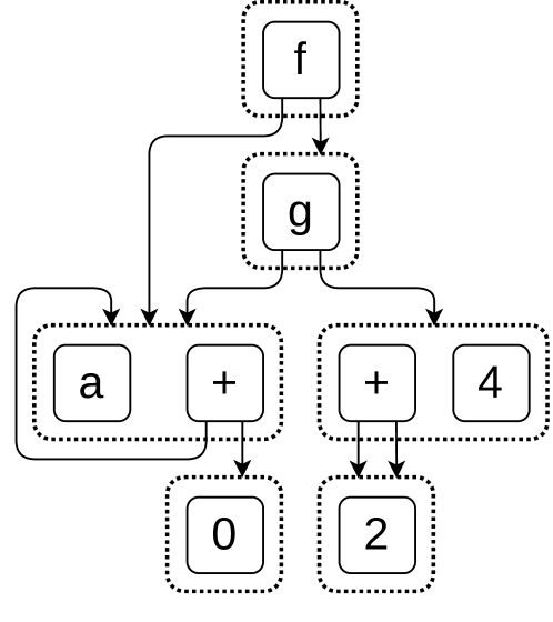
Figure 1: A e-graph model of the equalities $a+0=a$ and $2+2=4$ and the expression $f(a+0,g(a+0,2+2))$. Note that the top e-class contains both the expression $f(a+0,g(a+0,2+2))$ and the expression $f(a,g(a,4))$, which proves that these two expressions are equal modulo the equalities.

A congruence closure model is typically represented as an e-graph, which is a collection of e-nodes and e-classes. Each e-node represents a single function being applied and an e-class for each argument; each e-class, meanwhile, is a set of equivalent e-nodes. Any expression can be inserted into the e-graph by converting it recursively into e-nodes, while equalities can be added into the e-graph by merging the e-classes for the equality’s left and right hand side. For example, given the equalities $a+0=a$ and $2+2=4$, one can determine whether $f(a+0,g(a+0,2+2))=f(a,g(a,4))$ by inserting these two expression into an e-graph and then adding the two equalities. The resulting e-graph is shown in Figure 1. The two expressions end up in the same e-class, so they have been proven to be equal.

Congruence procedures must handle queries quickly, with tens or hundreds of thousands of equalities. The large number of equalities means that e-graphs can contain hundreds of thousands or even millions of e-nodes, with the resulting e-graph taking significant time to construct. A substantial literature [3, 6, 13] describes numerous optimizations to e-graphs. Past work shows that an e-graph for $n$ equalities can be constructed in $O(n\log n)$ time [14].

Congruence Proofs Proof certificates for e-graphs allow checking that two terms are equal without reconstructing the e-graph. Instead, for an equality $E_{1}=E_{2}$ witnessed by the e-graph, a proof certificate is a list of given equalities that can be applied in order, one after another, as rewrite rules to transform $E_{1}$ into $E_{2}$. Some of these equalities are applied at the root of the expression being rewritten, while others apply to subexpressions (via congruence). In our running example, we can prove $f(a+0,g(a+0,2+2))=f(a,g(a,4))$ as follows:

$$\begin{array}[]{l}f(a+0,g(a+0,2+2))\\[4.0pt] \;\;\;\;\;\;\xrightarrow{a+0=a}f(a,g(a+0,2+2))\\[4.0pt] \;\;\;\;\;\;\;\;\;\;\xrightarrow{2+2=4}f(a,g(a+0,4))\\[4.0pt] \;\;\;\;\;\;\;\;\;\;\;\;\;\;\xrightarrow{a+0=a}f(a,g(a,4))\\[4.0pt] \end{array}$$

Note that some equalities may be reused, as in this example.

Over time, proof certificates have grown increasingly important. In SMT solvers, proof certificates correspond to conflict clauses and enable non-chronological backtracking, a key component of modern SMT solvers [15]. In proof automation, proof certificates bridge foundational logics and unverified automated theorem provers, as in the “hammer” style of proof tactics [10]. In equality saturation engines, replaying proof certifications enables the combination of slow verification procedures with fast equality saturation engines.

To produce proofs certificates, e-graph implementations maintain a spanning tree for each e-class, with each edge of the tree justifying the equality of the two e-nodes it connects [16]. This justification is either one of the (quantifier-free) equalities provided as input or a congruence edge that refers to other connected nodes in the tree. This spanning tree is maintained alongside the union-find structure used for efficiently merging e-classes, so there is no algorithmic overhead to maintaining it. Producing a proof for the equality of two e-nodes in the same e-class is then a simple recursive procedure which traverses the path between two e-nodes, recursively finding subproofs for each congruence edge. In a spanning tree, there is a unique path between any two e-nodes, so this recursive algorithm is quite fast, taking $O(n\log n)$ time for $n$ equalities.

Shrinking Congruence Proofs Most uses of proof certificates, including generating conflict clauses and replaying and checking proofs, take longer as more unique equalities are used in the proof certificate. The standard approach to finding smaller proof certificates, implemented in SMT solvers such as Z3 [5], is based on the observation [16] that proof certificates can contain redundant equations; for example, if the given equalities include $a=b$, $a=c$, and $b=c$, a proof certificate may include all three. By attempting to re-prove the same equation while excluding one of the equalities, a proof certificate can thereby be shrunk. If the initial proof certificate has length $k$, this proof reduction procedure takes $O(k^{2}\log k)$ (as checking the validity of each new proof takes $O(k\log k)$ time using an e-graph).

This state of the art algorithm is limited in two ways. First, when $k\in o(\sqrt{n})$, it introduces an asymptotic slowdown over the rest of the congruence closure algorithm, which can answer queries and generate proofs in $O(n\log n)$ time (where $n$ is the number of equalities). Second and more importantly, proof reduction is ultimately limited by the choice of the proof to reduce. Since proof reduction is too slow to consider the entire e-graph, a valid initial proof is generated before applying proof reduction, discarding many (potentially useful) equalities right away. This means that, while it results in shorter proof certificates, those proof certificates are still longer than optimal. This paper addresses both concerns.

III Optimal DAG Size

Because proof certificates often contain repeated subproofs, we propose a measure for a proof’s size in terms of the number of unique equalities it uses. We call this measure DAG size because equalities may be reused in the proof. DAG size is also the same as the size of a conflict set in the context of SMT solvers. The problem of finding a proof of minimal DAG size is also NP-complete [12]. This section formalizes a DAG size measure of proof length which accounts for subproof reuse, and gives an ILP formulation for finding the proof of optimal DAG size.

III-A C-graphs

Traditionally, each equivalence class in an e-graph is represented by a spanning tree. Each edge in the spanning tree is either a single equality between two terms or equality via congruence. Any additional equalities between nodes already connected are discarded, since there is already a way to prove the two terms are equal. However, these equalities may enable a significantly smaller proof. For example, an e-graph can be constructed from the equalities $a=b$, $b=c$, and $a=c$. The e-graph constructs a spanning tree with edges $a=b$ and $b=c$, discarding $a=c$. Now the e-graph will admit a proof between $a$ and $c$ that has a size of $2$.

Since these additional equalities can be used to produce shorter proofs, our algorithm requires storing them. We call the resulting structure a c-graph, which maintains a graph, not a spanning tree, for each equivalence class. Storing these additional edges merely requires recording information on every e-graph merge operation, so can be done without changing the complexity of the congruence closure algorithm. The c-graph can be substituted directly for an e-graph without changing the complexity of the congruence closure algorithm. In practice, a c-graph uses the same representation and algorithms as an e-graph, but additionally has an adjacency list for each node storing this graph of equalities. In the context of producing proofs, we define a simple version of a c-graph below:

Definition 1.

A c-graph is an undirected graph $G=(V,E)$, where nodes $V$ represent expressions and edges $E$ represent equalities, along with a justification $j(e)$ for edge $e$. A justification is either an equality $v_{1}=v_{2}$ between the vertices or a congruence subproof $c_{1}=c_{2}$, where $c_{i}$ is a child of $v_{i}$.

For convenience, we write $C$ for the set of congruence edges in $E$. An edge justified by an equality connects the left and right-hand sides of the equality directly, while an edge justified by a congruence $c_{1}=c_{2}$ connects terms which are equal by congruence over $c_{1}$ and $c_{2}$ (e.g. $f(c_{1})$ and $f(c_{2})$). If two terms are equal due to the congruence of multiple children, the c-graph contains one congruence edge per argument (one per child). This keeps the encoding simple, as each congruence edge corresponds to one proof of congruence. All functions have a bounded arity, so this transformation does not affect complexity results.

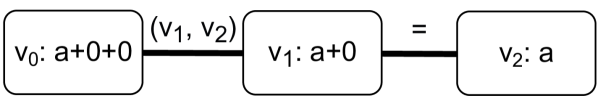
Figure 2: A c-graph proof that $a+0+0=a$. There is one congruence edge $(v_{0},v_{1})$ with $j((v_{0},v_{0}))=(v_{1},v_{2})$. Since $v_{0}$ and $v_{2}$ are e-connected, the proof holds.

For a c-graph to be a valid proof, all congruence edges must refer to e-connected nodes:

Definition 2.

A congruence edge $e\in E$ with $j(e)=(c_{1}=c_{2})$ is valid if the congruent children $c_{1}$ and $c_{2}$ are e-connected in the reduced c-graph $(G^{\prime},j)$, where $G^{\prime}=(V,E\setminus\{e\})$. All non-congruence edges are valid.

Definition 3.

Two vertices $v_{s}$ and $v_{t}$ are e-connected in a c-graph $(G,j)$ if there is a path between them consisting of valid edges in $E$.

A c-graph then proves $s=t$ if the corresponding vertices $v_{s}$ and $v_{t}$ are e-connected. The particular path showing that $v_{s}$ and $v_{t}$ are e-connected, along with proofs for each congruence edge along the path, represents a particular proof. The definition of e-connectedness and edge validity are mutally recursive; the base case occurs when two vertices are connected by a set of non-congruence edges.

The c-graph structure allows for a simple definition of the DAG size metric:

Definition 4.

The DAG size of a c-graph $(G,j)$ is $|E\setminus C|$, the number of non-congruence edges it contains.

Each non-congruence edge $e\in E\setminus C$ could also be assigned a positive, real-numbered weight $w(e)$, giving a weighted DAG size: $\sum_{e\in E\setminus C}w(e)$. Applications could leverage these weights in order to sample proofs that minimize an alternative objective function, such as the run-time of verifying the steps of the proof. The algorithms in this paper easily support weighted DAG size, but we will use the simpler definition of DAG size with each non-congruence edge assigned a weight of 1.

III-B Minimal DAG Size

$$\begin{array}[]{lll}\textsc{Edges}&S[i,j]\leq(i,j)\in E\setminus C&S[i,j]=S[j,i]\\[12.0pt] \textsc{Congruence}&M[i,j,l,r]\leq(i,j)\in E\land j((i,j))=(l=r)&M[i,j,l,r]=M[j,i,r,l]\\[12.0pt] \textsc{Paths}&P[i,i,j]=0&P[i,k,j]\leq V[i,j]\\[5.0pt] &C[i,j]=\sum_{k}P[i,k,j]&P[i,k,j]\leq C[k,j]\\[12.0pt] \textsc{Validity}&V[i,j]\leq S[i,j]+\sum_{l,r}M[i,j,l,r]\\[12.0pt] \textsc{No Cycles}&0\leq D[i,j]\leq\ell&D[i,j]\geq 1\text{ if }i\neq j\\[5.0pt] &(1-P[i,k,j])\ell+(D[i,j]-D[k,j])\geq D[i,k]\\[5.0pt] &(1-M[i,j,l,r])\ell+D[i,j]\geq D[l,r]\\[12.0pt] \textsc{Goal}&C[v_{s},v_{t}]=1&\min\sum_{i,j}S[i,j]\\ \end{array}$$

Figure 3: An integer linear programming formulation of the minimum DAG size problem. Variables $S$, $M$, $V$, and $P$ are sets of boolean variables, while $D$ is integer-valued. Variables are indexed by $i$, $j$, and $k$, which represent nodes in the c-graph. Decision variables $S$ and $M$ define which non-congruence and congruence edges of $E$ are selected respectively. $\ell=|C|^{|C|+1}|E|$ bounds the maximum length of a valid non-cyclic path.

The key to finding shorter proofs is to keep track of a c-graph of possible proofs during congruence closure, from which a short proof can eventually be extracted. Traditional congruence closure algorithms store only one proof of equality between any two terms (they generate c-graphs shaped like forests) because they discard any equalities they discover between already-equal terms. Instead, we will store these redundant edges, producing a c-graph shaped like a full graph, and will then later search this c-graph for a sub-c-graph of minimal size. We will also discover any extra opportunities for proofs of congruence between terms, adding these to the c-graph as congruence edges.

Definition 5.

Consider a c-graph $(G,j)$, all of whose edges are valid. We write $(G^{\prime},j)\subseteq(G,j)$ when $G^{\prime}\subseteq G$ and all edges in $(G^{\prime},j)$ are valid.

The goal is then to find the sub-c-graph of minimal size in which two terms $s$ and $t$ remain e-connected.

Definition 6 (The Minimum DAG size Problem).

Given a c-graph $(G,j)$ and two e-connected terms $s$ and $t$, find a $(G^{\prime},j)\subseteq(G,j)$ in which $s$ and $t$ remain e-connected with minimal DAG size.

Note that a sub-c-graph is defined by which edges in $G$ it keeps; this allows us to phrase the minimum DAG size problem as an integer linear programming problem with one decision variable per edge in $E$. The full linear programming problem is given in Figure 3. It defines selected edges via $S$ and $M$, paths $P$ and e-connectedness $C$ (via edge validity $V$), and breaks cycles using distance measure $D$; it is similar to the standard formulation of graph connectedness as an ILP problem, except with extra constraints for the validity of congruence edges. These constraints require the selected edges $S$ and $M$ to form a sub-c-graph of $(G,j)$ with all edges valid. Finally, $v_{s}$ and $v_{t}$ are asserted to be e-connected to ensure that the sub-c-graph proves $s=t$ and then DAG size is minimized. While this ILP formulation is solvable by industry-standard ILP solvers for very small instances, it is NP-complete in general [12].

IV Optimal Tree Size

What makes the minimal DAG size problem NP-complete is the fact that the e-connectedness of multiple congruence edges can rely on the same edges. This sharing means that the cost of using a congruence edge depends on equalities other congruence edges rely on—global information about the sub-c-graph of the solution as a whole. Instead of finding the optimal solution, we optimize for a different metric to achieve a practical algorithm for proof length minimization. The distance metric $D[i,j]$ in the ILP formulation, which we call the tree size of a c-graph, is an effective metric for this purpose.

The tree-size of a c-graph is computed by summing the length of the proof, without sharing. Specifically, given a c-graph $(G,j)$ that proves $s=t$, its tree size is the tree size of the path from $v_{s}$ to $v_{t}$:

Definition 7.

Consider a path $P$ that e-connects $v_{i}$ to $v_{j}$ in a c-graph. The tree size of $P$ is the number of non-congruence edges in $P$ plus, for each congruence edge justified by $(v_{l}=v_{r})$, the tree size of the path from $v_{l}$ to $v_{r}$.

If a c-graph has minimal DAG size, its DAG size is the number of non-congruence edges in the graph. Its tree size, meanwhile, may count each more than once, so presents an upper bound on the DAG size. We can thereby hope that the c-graph of minimal tree size will also have a small DAG size.

Definition 8 (The Minimum Tree Size Problem).

Given a c-graph $(G,j)$ that proves $s=t$, find the $(G^{\prime},j)\subseteq(G,j)$ that proves $s=t$ and has minimal tree size.

IV-A Minimum Proof Tree Size Algorithm

Unlike DAG size, tree size does not have the problem of shared edges. Finding a proof of optimal tree size thus does not require global reasoning about the surrounding context: using the same edges with another part of the proof does not reduce the tree size. As a result, it is possible to solve the minimum tree size problem in polynomial time.

Finding a proof of optimal tree size is not a simple graph search. The key problem is that congruence edges may contain other congruence edges in their subproofs, and the tree size of those subproofs is initially unknown. Moreover, often a congruence edge $(v_{1},v_{2})$ can be proven in terms of another congruence edge $(v_{3},v_{4})$ and vice versa. Our algorithm tackles this problem by computing the size of proofs of congruence bottom up, in multiple passes. At the $i$-th pass, it constructs proofs of equalities between vertices where congruence subproofs only go $i$ layers deep. These proofs form an upper bound on the optimal tree size, decreasing in size until the optimal proof is found. When the algorithm reaches a fixed point, the proof of optimal tree size is discovered. The algorithm for finding the size of the optimal proof is given in Figure 4. With more bookkeeping, it can be easily extended to yield the specific proof the optimal size corresponds to.

⬇

1 def optimal_tree_size(start, end):

2 for i in G.vertices:

3 dist[(i, i)] = 0

4

5 for ($\ell$, $r$) in E \ C:

6 dist[$\ell$, $r$] = 1

7

8 for i in range(|C|):

9 for ($\ell$, $r$) in C:

10 dist[$\ell$, $r$] = shortest_path($\ell$, $r$, dist)

11 return shortest_path(start, end, weights=dist)

Figure 4: Pseudocode for the optimal proof tree size algorithm. The algorithm keeps a dictionary $dist[a,b]$, the length of the shortest tree size from $a$ to $b$ found so far.

In each pass, this algorithm computes the shortest path for each proof of congruence. Non-congruence edges have a weight of 1, and congruence edges are initialized to have infinite weight. A fixed point is guaranteed after $|C|$ iterations, because each subproof for a congruence edge $e$ cannot use the same edge $e$ again (else its tree size would increase). The overall running time of the algorithm is bounded by $O(|C|^{2}|E|)$, with $|C|^{2}$ being the number of calls to the shortest path algorithm and $|E|$ being the complexity of finding a shortest path given the weights. Since there may be $n^{2}$ congruence edges for $n$ nodes in the graph, the overall running time is also bounded by $O(n^{5})$. However, in practice the number of congruence edges is some constant multiple of $n$, and in this case the running time is $O(n^{3})$.

V Greedy Optimization of Proof Tree Size

The optimal algorithm of Section IV finds the proof with minimal tree size, but it does so at an unacceptable cost: its running time dominates the $O(n\log n)$ running time of congruence closure itself [1]. In the context of c-graphs, $n=|E\setminus C|$, the set of input equalities to congruence closure. This section thus proposes a greedy algorithm for proof tree size, which reduces tree size and DAG size significantly in practice, though it is not optimal with respect to either metric.

V-A Greedy Optimization

The key insight behind the greedy algorithm is that the multiple passes of the optimal algorithm are only necessary to compute the minimal cost of congruence edges. If the tree size for each congruence edge were known, the proof with optimal tree size could be found by a simple shortest path algorithm. The greedy algorithm is a simple breadth-first search shortest path algorithm that takes estimated costs for congruence edges as an input. The closer the estimates are to the proof of optimal tree size, the better the results of the greedy algorithm.

Defer for now the challenge of estimating the tree size for each congruence edge, and focus on the greedy algorithm itself. The algorithm is simple: use a breadth-first search to choose a path from the start vertex $s$ to the end vertex $t$ of minimal length, using the estimates for each congruence edge. However, those estimates may not be optimal, so the algorithm then recurses for each congruence edge. Note the difference between the optimal algorithm (which first optimizes congruence edges) and the greedy algorithm (which first finds a shortest path). If the recursion were performed until all congruences are optimized, this algorithm would take time $O(|C|(n+|C|))$, which is still too high compared to the $O(n\log(n))$ runtime of congruence closure. Instead, only $T$ expansions of congruence edges are permitted; in practice, we choose $T=10$, which seems to work well. After $T$ expansions, there may be sub-proofs which have not been generated. In this case, the algorithm defaults to a generic proof production algorithm for the remaining sub-proofs [16]. Figure 5 lists the greedy algorithm.

⬇

1 def greedy(start, end, pf_size_estimates):

2 todo = Queue((start, end))

3 fuel = $T$

4

5 while len(todo) > 0:

6 (start, end) = todo.pop()

7 path = shortest_path(start, end, pf_size_estimates)

8 for edge in path:

9 match edge:

10 congruence($\ell$, $r$) ->

11 if fuel > 0:

12 todo.push($\ell$, $r$)

13 fuel = fuel - 1

14 else:

15 add_to_proof(unoptimized_proof($\ell$, $r$))

16 axiom(a) ->

17 add_to_proof(a)

Figure 5: Pseudocode for the greedy optimization of proof tree size. The algorithm either recurs for congruence edges if fuel allows, or it uses the estimates for each congruence edge. Unlike TreeOpt, the algorithm is top-down and terminates after $T$ steps.

V-B Estimating Tree Sizes

The main challenge to instantiating the greedy algorithm is generating size estimates for congruence edges. However, there is a simple way to do so: reduce the c-graph to a forest $(G_{t},j)$ with one tree per connected component, in such a way that all edges remain valid. Luckily, the traditional congruence closure proof production algorithm generates such reduced c-graphs by omitting any unions which connect already-equal terms. Now, the tree size of a proof of congruence can be estimated by directly calculating the tree size of a proof in the reduced instance. In such a reduced c-graph, there is only one possible path between any two nodes, so the proof is unique.

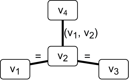
Figure 6: An example reduced c-graph with a single congruence edge. The root of the tree is the vertex labeled $v_{4}$ at the top, and there is a single congruence edge $(v_{1},v_{2})$ in the spanning tree. The proof of congruence between vertices $1$ and $2$ has a tree size of two because the proof between the congruent children involves two equalities.

Computing the tree sizes of all proofs in the reduced c-graph requires some care to stay within the necessary asymptotic bounds. First, each tree in $(G_{t},j)$ is arbitrarily rooted. Given a vertex $a$, let size[$a$] be the size of the proof between $a$ and the root of its tree. Then the tree size of the proof between any two vertices $a$ and $b$ can be calculated

$$\texttt{size[$a$] + size[$b$] - 2 * size[lca($a$, $b$)]},$$

where lca computes the least common ancestor of $a$ and $b$ in the tree. The lca function can be pre-computed for all relevant proofs in $O(n)$ time using Tarjan’s off-line algorithm [17].

⬇

1

2def path_compress(vertex):

3 if parent[vertex] != vertex:

4 path_compress(parent[vertex])

5 parent[vertex] = parent[parent[vertex]]

6 size[vertex] = size[vertex] + size[parent[vertex]]

7

8def traverse_to_ancestor(v, ancestor):

9 while parent[vertex] != ancestor:

10 edge = parent_edge(parent[vertex], G)

11 parent[edge.start] = edge.end

12 if is_congruence(edge):

13 traverse(j(edge).start, j(edge).end)

14 estimate_size(edge)

15 path_compress(vertex)

16

17def traverse(start, end):

18 path_compress(start)

19 path_compress(end)

20 ancestor = argmin(

21 (lca(start, end), parent[start], parent[end]),

22 distance_to_root)

23 path_compress(ancestor)

24

25 # Ensure that start, end, and their lca share a parent

26 traverse_to_ancestor(start, ancestor)

27 traverse_to_ancestor(end, ancestor)

28 estimate_tree_size(start, end)

29

30def estimate_tree_size(start, end):

31 tree_size[(start, end)] = size[start] + size[end]

32 - 2*size[lca(start, end)]

33

34def estimate_size(edge):

35 match edge:

36 congruence(left, right) ->

37 size[edge.start] = tree_size[(left, right)]

38 axiom(a) ->

39 size[edge.start] = 1

40

41for i in G.vertices:

42 parent[i] = i

43 size[i] = 0

44

45for (start, end) in congruence_edges(G):

46 traverse(start, end)

Figure 7: Pseudocode for computing tree sizes of all congruence proofs given $(G_{t},j)$. The algorithm efficiently computes these tree sizes by storing a union-find datastructure that keeps track of size, the size of the proof between a node and it’s parent. Computing the size of a proof involves traversing the proof, updating the union-find whenever the size of a sub-proof is discovered. The pseudocode uses the function distance_to_root to denote the number of edges from $v$ to the root of its tree. It also makes use of lca, a function that returns the lowest common ancestor of two vertices.

Figure 7 shows the pseudocode for calculating proof tree sizes given $(G_{t},j)$. To avoid an infinite loop in proof length calculation, the algorithm builds each tree in $(G_{t},j)$ incrementally using a union-find structure (using the parent array). Consider the example in Figure 6, in which the path to the root node $v_{4}$ contains a congruence edge. The tree size of the proof between nodes $v_{2}$ and $v_{4}$, written tree_size($v_{2}$, $v_{4}$), involves calculating the size of the congruence proof tree_size($v_{1}$, $v_{3}$). So tree_size($v_{2}$, $v_{4}$) cannot be computed using $v_{4}$ as the root of the tree, since the path to the root involves the congruence edge. Instead, the algorithm uses least common ancestor $v_{2}$ to compute tree_size($v_{1}$, $v_{3}$). Because the proof is e-connected, any congruence edges on the path to the least common ancestor can be computed recursively without diverging.

Each congruence edge results in at most one recursive call to traverse, while non-congruence edges are added to the union-find data structure directly. Ultimately, each edge in the c-graph contributes at most five union-find operations: three find operations at the start of tree_size, one union operation to add it to the union-find data structure, and one more find in traverse_to_ancestor. A sequence of $m$ operations on a union-find data structure with $h$ nodes can be executed in $O(m\log(h))$ time [18]. This means the overall cost of estimating sizes for congruence edges is $O(n\log(n))$ since $n$ bounds both $m$ and $h$ (recall $n=|E\setminus C|$). Adding on $O(n+|C|)$ cost for the greedy algorithm itself yields an overall runtime of $O(n\log(n)+n+|C|)=O(n\log(n)+|C|)$. Limiting the number of congruence edges $C$ to a multiple of $n$ results in a $O(n\log(n))$ runtime, introducing no asymptotic overhead compared to congruence closure alone.

VI Evaluation

This section compares an implementation of our greedy proof generation algorithm in the egg equality saturation toolkit [3] to Z3’s proof generation [19]. As described in Section II, Z3 applies proof reduction to the first proof it finds, which substantially reduces proof size. Our greedy approach instead attempts to extract a minimal proof from the e-graph. We found that, even without a proof reduction post-pass, our greedy approach can quickly find significantly smaller proofs than Z3 (Figure 8).

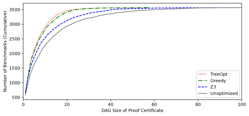
Figure 8: This CDF compares the unoptimized (gray solid), Z3 (blue dashed), greedy (green dash-dotted), and TreeOpt (red dotted) proof generation algorithms on the same 3 571 benchmarks where Z3 does not time out. Each line shows the number of benchmarks whose proofs are at most the size indicated on the horizontal axis. Our greedy approach (green) closely tracks the size of TreeOpt’s (red) proof certificates, showing that its certificates are difficult to shrink further. Five outliers with an unoptimized DAG size of more than 100 are omitted.

VI-A Comparing egg to Z3

We use Z3 version 4.8.12 and egg version 0.7.1 compiled with Rust 1.51.0. egg is a state-of-the-art equality saturation library that implements the rebuilding algorithm for speeding up equality saturation workloads. It is used by projects like Herbie [20], Ruler [21] and Szalinski [22]. Z3 is a state-of-the-art automated theorem prover and is optimized for theorem proving workloads. To create a realistic benchmark set, we used the Herbie 1.5 numerical program synthesis tool [20]. Herbie uses equality saturation for program optimization and comes with a standard benchmark suite of programs drawn from textbooks, research papers, and open-source software. We extracted Herbie’s set of quantified equalities and recorded all inputs and outputs from its equality saturation procedure. This results in 3 760 input/output pairs, of which we focus on the 3 571 where Z3 did not produce an answer after 2 minutes.

For the Z3 baseline, we converted each input/output pair into a satisfiability query by asserting each quantified equality (with a trigger for the left hand side of the equality) and then asserting that the input and output are not equal. Z3 then attempts to prove the input and output are equal using an e-graph and the quantified equalities (the theory of uninterpreted functions). We then computed the DAG size by counting the number of calls to its quant-inst command [23] in its proof scripts. We ran egg exactly how it is used by Herbie, and then optimized proof length using the greedy algorithm of Section V and measured DAG size by counting proof nodes. Z3 times out after 2 minutes for 5.0% of the input/ouput pairs, and completes in 213.25 milliseconds on average for the remainder. egg does not time out, and runs for an average of 39.57 milliseconds. To measure DAG size for the resulting proofs, we ran both egg and Z3 in proof-producing mode and examined the resulting proofs.

Figure 8 contains the results: the proofs produced by egg are 72.8% as big as Z3’s on average, despite Z3’s use of a proof reduction algorithm. Moreover, the effect of proof length optimization is greater for longer proofs: queries with Z3 DAG size over 10 see an average 36.0% reduction, while queries with Z3 DAG size over 50 see an average 49.7% reduction.

TABLE I: Data comparing egg to Z3 using different proof production algorithms: egg with proofs of optimal tree size, egg with greedy optimization, egg with traditional proof reduction (see section II), Z3, and egg without any optimization. Note that proof reduction’s analysis is in terms of $k$, the size of the unoptimized proof, while $n$ is the size of the entire c-graph instance. In practice, $k$ is often small relative to $n$.

Algorithm	TreeOpt	Ave Time (ms)	Complexity
TreeOpt	100.0%	1008.60	$O(n^{3})$
Greedy	105.9%	39.33	$O(n\log(n))$
Egg Reduc.	138.7%	23.01	$O(n\log(n)+k^{2}\log(k))$
Z3	147.3%	130.69	$O(n\log(n)+k^{2}\log(k))$
Egg	185.9%	22.15	$O(n\log(n))$

TABLE II: RTL design benchmark results. Total runtime includes equality saturation and proof production runtimes but excludes any formal verification time.

	Tree Size			DAG Size			Runtime (sec)
Benchmark .	. Orig	Greedy	Reduce	.. Orig	Greedy	Reduce	.. Total	. Proof	. Proof %
Datapath 1	174	90	48%	67	61	9%	37.5	2.58	7%
Datapath 2	561	92	84%	98	46	53%	34.5	2.08	6%
Datapath 3	14	13	7%	13	12	8%	5.13	0.49	9%
Datapath 4	4402	202	95%	223	120	46%	76.4	32.80	43%
Datapath 5	271	95	65%	101	72	29%	105	0.18	0.2%
Datapath 6	155	83	46%	67	49	27%	280	168.00	60%

VI-B Detailed Analysis

In this section, we perform a more detailed ablation study comparing egg’s results using different algorithms. We implement proof reduction for egg and the optimal tree width algorithm described in Section IV. The ILP solution is not feasible to run, so we use Z3 as a baseline.

Table I summarizes the results. Z3 and egg are optimized for different workloads and so use different underlying congruence closure algorithms, and so produce different proofs. Using proof reduction, egg finds slightly shorter proofs than Z3. It also performs better than Z3-style proof reduction implemented in egg. Using the greedy algorithm, egg finds proofs which are even shorter, and which are also quite close to proofs of optimal tree size. The data in Table I consists of the 3 571 out of 3 760 where Z3 did not time out, the same set used in Figure 8.

While we would ideally use the minimal DAG size proofs as a baseline in our evaluation, we found the ILP formulation was infeasible to run on real queries. However, the $O(n^{5})$ TreeOpt algorithm, which runs in $O(n^{3})$ time when the number of congruences is bounded, performs well enough to run on all of the examples. We found that in 81.1% of these cases, the greedy algorithm in fact found the proof with optimal tree size. Moreover, across all of these benchmarks our greedy algorithm’s overall performance closely tracks that of TreeOpt, showing that the greedy algorithm’s proof certificates are difficult to shrink further.

VI-C Case Study

Typically, proof production is necessary in equality saturation to perform translation validation. In this case, the shorter proofs produced by proof length optimization reduce the number of translation validation steps that must be performed and thus result in faster end-to-end results. A practical application that benefits from this reduction is hardware optimization performed using egg by researchers at Intel Corporation [11]. Translation validation is used to ensure that the egg optimized hardware designs are formally equivalent to the input. Extremely high assurance is needed for hardware designs because of the high cost of actual hardware manufacturing. For each step in the tree proof two Register Transfer Level (RTL) designs are generated, which are proven to be formally equivalent by Synopsys HECTOR technology, an industrial formal equivalence checking tool. The intermediate steps generate a chain of reasoning proving the equivalence of the input and optimized designs, necessary because the tools can fail to prove equivalence of significantly transformed designs. The tree proof is used to ensure that HECTOR can prove each step with no user input as it is a simpler check than a DAG proof step.

Figure 9: Dataflow graph of an optimized multiple constant multiplication circuit design generated by egg.

The results of evaluating this paper’s greedy optimization algorithm on six Intel-tested RTL design benchmarks are shown in Table II. On average, proof lengths decreased by $29\%$, with the best case showing a $53\%$ reduction, while proof production took only $34$ seconds on average, miniscule compared to multi-hour translation validation times. Moreover, these reductions in proof length resulted in shorter translation validation times. The optimized constant multiplication hardware design descibed in Figure 9 was generated by egg, starting from an initial naive implementation. Running the complete verification flow for the original and greedy proofs, the runtime was reduced from $4.7$ hours to $2.3$ hours. In more complex examples we expect that days of computation could be saved. For parameterizable RTL, where a design must typically be re-verified for every possible paramterization, these gains add up quickly.

VII Conclusion and Future Work

This paper examined the problem of finding minimal congruence proofs from first principles. Since finding the optimal solution is infeasible, we introduced a relaxed metric for proof size called proof tree size, and gave an $O(n^{5})$ algorithm for optimal solutions in that metric. While the optimal algorithm is too expensive in practice, it provides a reasonable baseline for small congruence problems, and inspired a practical $O(n\log(n))$ greedy algorithm which generates proofs which are 107.8% as big on average.

We implemented proof generation in the egg equality saturation toolkit, making it the first equality saturation engine with this capability. Since equality saturation toolkits—unlike SMT solvers—support optimization directly, this opens the door to certifying the results of much recent work in optimization and program synthesis [3, 21, 24, 20, 25, 26, 22].

Looking forward, we are especially eager for the community to explore more applications of proof certificates in congruence closure procedures. For example, it should be possible to use proofs to tune rewrite rule application schedules in e-matching, improve debugging of subtle equality saturation issues, and enable equality-saturation-based “hammer” tactics in proof assistants. It may also be possible to further improve on the greedy proof generation algorithm with better heuristics for estimating proof sizes, or to enable more efficient prover state serialization via smaller proofs.

VIII Acknowledgements

This work was supported by the Applications Driving Architectures (ADA) Research Center, a JUMP Center co-sponsored by SRC and DARPA and supported by the National Science Foundation under Grant No. 1749570.

References

- [1] C. G. Nelson, “Techniques for program verification,” Ph.D. dissertation, Stanford, CA, USA, 1980, aAI8011683.
- [2] R. Tate, M. Stepp, Z. Tatlock, and S. Lerner, “Equality saturation: A new approach to optimization,” in Proceedings of the 36th Annual ACM SIGPLAN-SIGACT Symposium on Principles of Programming Languages, ser. POPL ’09. New York, NY, USA: ACM, 2009, pp. 264–276. [Online]. Available: http://doi.acm.org/10.1145/1480881.1480915
- [3] M. Willsey, C. Nandi, Y. R. Wang, O. Flatt, Z. Tatlock, and P. Panchekha, “Egg: Fast and extensible equality saturation,” Proc. ACM Program. Lang., vol. 5, no. POPL, jan 2021. [Online]. Available: https://doi.org/10.1145/3434304
- [4] C. Barrett, C. L. Conway, M. Deters, L. Hadarean, D. Jovanović, T. King, A. Reynolds, and C. Tinelli, “Cvc4,” in Proceedings of the 23rd International Conference on Computer Aided Verification, ser. CAV’11. Berlin, Heidelberg: Springer-Verlag, 2011, p. 171–177.
- [5] L. De Moura and N. Bjørner, “Z3: An efficient smt solver,” in Proceedings of the Theory and Practice of Software, 14th International Conference on Tools and Algorithms for the Construction and Analysis of Systems, ser. TACAS’08/ETAPS’08. Berlin, Heidelberg: Springer-Verlag, 2008, pp. 337–340. [Online]. Available: http://dl.acm.org/citation.cfm?id=1792734.1792766
- [6] L. Moura and N. Bjørner, “Efficient e-matching for smt solvers,” in Proceedings of the 21st International Conference on Automated Deduction: Automated Deduction, ser. CADE-21. Berlin, Heidelberg: Springer-Verlag, 2007, p. 183–198. [Online]. Available: https://doi.org/10.1007/978-3-540-73595-3_13
- [7] D. Winterer, C. Zhang, and Z. Su, “Validating smt solvers via semantic fusion,” in Proceedings of the 41st ACM SIGPLAN Conference on Programming Language Design and Implementation, ser. PLDI 2020. New York, NY, USA: Association for Computing Machinery, 2020, p. 718–730. [Online]. Available: https://doi.org/10.1145/3385412.3385985
- [8] D. Oe, A. Reynolds, and A. Stump, “Fast and flexible proof checking for smt,” in Proceedings of the 7th International Workshop on Satisfiability Modulo Theories, ser. SMT ’09. New York, NY, USA: Association for Computing Machinery, 2009, p. 6–13. [Online]. Available: https://doi.org/10.1145/1670412.1670414
- [9] L. de Moura and N. Bjørner, “Proofs and refutations, and Z3,” in Proceedings of the LPAR 2008 Workshops, Knowledge Exchange: Automated Provers and Proof Assistants, and the 7th International Workshop on the Implementation of Logics, Doha, Qatar, November 22, 2008, ser. CEUR Workshop Proceedings, P. Rudnicki, G. Sutcliffe, B. Konev, R. A. Schmidt, and S. Schulz, Eds., vol. 418. CEUR-WS.org, 2008. [Online]. Available: http://ceur-ws.org/Vol-418/paper10.pdf
- [10] L. Czajka and C. Kaliszyk, “Hammer for coq: Automation for dependent type theory,” Journal of Automated Reasoning, vol. 61, 06 2018.
- [11] S. Coward, G. A. Constantinides, and T. Drane, “Automatic datapath optimization using e-graphs,” vol. abs/2204.11478, 2022. [Online]. Available: https://arxiv.org/abs/2204.11478
- [12] A. Fellner, P. Fontaine, and B. Woltzenlogel Paleo, “Np-completeness of small conflict set generation for congruence closure,” Formal Methods in System Design, vol. 51, 12 2017.
- [13] Y. Zhang, Y. R. Wang, M. Willsey, and Z. Tatlock, “Relational e-matching,” Proc. ACM Program. Lang., vol. 6, no. POPL, jan 2022. [Online]. Available: https://doi.org/10.1145/3498696
- [14] P. J. Downey, R. Sethi, and R. E. Tarjan, “Variations on the common subexpression problem,” J. ACM, vol. 27, no. 4, p. 758–771, oct 1980. [Online]. Available: https://doi.org/10.1145/322217.322228
- [15] H. Ganzinger, G. Hagen, R. Nieuwenhuis, A. Oliveras, and C. Tinelli, “Dpll( t): Fast decision procedures,” in CAV, 2004.
- [16] R. Nieuwenhuis and A. Oliveras, “Proof-producing congruence closure,” in Proceedings of the 16th International Conference on Term Rewriting and Applications, ser. RTA’05. Berlin, Heidelberg: Springer-Verlag, 2005, p. 453–468. [Online]. Available: https://doi.org/10.1007/978-3-540-32033-3_33
- [17] H. N. Gabow and R. E. Tarjan, “A linear-time algorithm for a special case of disjoint set union,” in Proceedings of the Fifteenth Annual ACM Symposium on Theory of Computing, ser. STOC ’83. New York, NY, USA: Association for Computing Machinery, 1983, p. 246–251. [Online]. Available: https://doi.org/10.1145/800061.808753
- [18] R. E. Tarjan, “Efficiency of a good but not linear set union algorithm,” J. ACM, vol. 22, no. 2, p. 215–225, Apr. 1975. [Online]. Available: https://doi-org.offcampus.lib.washington.edu/10.1145/321879.321884
- [19] L. de Moura and N. Bjørner, “Proofs and refutations, and z3,” vol. 418, 01 2008.
- [20] P. Panchekha, A. Sanchez-Stern, J. R. Wilcox, and Z. Tatlock, “Automatically improving accuracy for floating point expressions,” SIGPLAN Not., vol. 50, no. 6, p. 1–11, Jun. 2015. [Online]. Available: https://doi.org/10.1145/2813885.2737959
- [21] C. Nandi, M. Willsey, A. Zhu, Y. R. Wang, B. Saiki, A. Anderson, A. Schulz, D. Grossman, and Z. Tatlock, “Rewrite rule inference using equality saturation,” Proc. ACM Program. Lang., vol. 5, no. OOPSLA, oct 2021. [Online]. Available: https://doi.org/10.1145/3485496
- [22] C. Nandi, M. Willsey, A. Anderson, J. R. Wilcox, E. Darulova, D. Grossman, and Z. Tatlock, “Synthesizing structured CAD models with equality saturation and inverse transformations,” in Proceedings of the 41st ACM SIGPLAN Conference on Programming Language Design and Implementation, ser. PLDI 2020. New York, NY, USA: Association for Computing Machinery, 2020, p. 31–44. [Online]. Available: https://doi.org/10.1145/3385412.3386012
- [23] S. Böhme, “Proof reconstruction for Z3 in Isabelle/HOL,” in 7th International Workshop on Satisfiability Modulo Theories (SMT ’09), 2009.
- [24] Y. Yang, P. M. Phothilimtha, Y. R. Wang, M. Willsey, S. Roy, and J. Pienaar, “Equality saturation for tensor graph superoptimization,” in Proceedings of Machine Learning and Systems, 2021.
- [25] A. VanHattum, R. Nigam, V. T. Lee, J. Bornholt, and A. Sampson, Vectorization for Digital Signal Processors via Equality Saturation. New York, NY, USA: Association for Computing Machinery, 2021, p. 874–886. [Online]. Available: https://doi.org/10.1145/3445814.3446707
- [26] Y. R. Wang, S. Hutchison, J. Leang, B. Howe, and D. Suciu, “SPORES: Sum-product optimization via relational equality saturation for large scale linear algebra,” Proceedings of the VLDB Endowment, 2020.