Interaction-controlled impurity transport in trapped mixtures of ultracold bosons

Abstract

We explore the dynamical transport of an impurity between different embedding majority species which are spatially separated in a double well. The transfer and storage of the impurity is triggered by dynamically changing the interaction strengths between the impurity and the two majority species. We find a simple but efficient protocol consisting of linear ramps of majority-impurity interactions at designated times to pin or unpin the impurity. Our study of this highly imbalanced few-body triple mixture is conducted with the multi-layer multi-configuration time-dependent Hartree method for atomic mixtures which accounts for all interaction-induced correlations. We analyze the dynamics in terms of single-particle densities, entanglement growth and provide an effective potential description involving mean-fields of the interacting components. The majority components remain self-trapped in their individual wells at all times, which is a crucial element for the effectiveness of our protocol. During storage times each component performs low-amplitude dipole oscillations in a single well. Unexpectedly, the inter-species correlations possess a stabilizing impact on the transport and storage properties of the impurity particle.

I Introduction

Tunneling of microscopic particles through a classically forbidden barrier is an exceptionally important quantum-mechanical phenomenon. It is a direct consequence of the particle-wave duality and the uncertainty principle. Tunneling has a wide range of real-world applications: it imposes a fundamental limit for the size of transistors [1] and lies at the heart of numerous technological devices such as the scanning tunneling microscope [2, 3], the tunnel diode [4], ultrasensitive magnetometers (SQUID) [5] and superconducting qubits [6]. The concept has been used to explain fundamental problems in physics, chemistry and biology with great success, including radioactive decay processes [7, 8], nuclear fusion [9], astrochemical synthesis [10], chemical reactions [11] and DNA mutations [12].

Tunneling can be observed on a macroscopic scale between two phase-coherent spatially overlapping matter waves [13], and has been detected via a current between two superconductors separated by a thin insulating layer (SJJ), even though no external voltage is applied (dc-Josephson effect). An external voltage gives then rise to a rapidly oscillating current (ac-Josephson effect). The Josephson effect [14, 15] was also reported for superfluid helium [16, 17, 18, 19], cavity polaritons [20] and ultracold atomic gases [21, 22, 23, 24, 25, 26, 27, 28]. The latter platform is of particular relevance for a quantitative analysis of the tunneling effect, as it provides an exquisite control over system parameters and versatile detection techniques [29]. Atomic Josephson junctions [30] have been suggested as a standard of chemical potential [31], to perform measurements of gravity [32, 33] and off-diagonal long-range order [34] with a high spatial resolution.

A double well loaded with a many-body ensemble of ultracold bosons, known as the bosonic Josephson junction (BJJ) [35, 36, 37], has drawn particular attention due to its fundamental nature and conceptual simplicity. Two wells separated by a barrier is a paradigmatic external potential to investigate tunneling dynamics [21, 22, 23, 24, 25, 26, 27, 28], interference of matter waves [38, 39, 23, 40, 41], the Shapiro [42, 43] and ratchet effects [44], macroscopic superposition states [45, 46, 47, 48, 49] and entanglement [50, 51, 52]. Furthermore, it serves as a prototype model for finite-size lattices [53, 54, 55, 56, 57].

BJJ can be understood in a two-mode approximation (lowest band Bose-Hubbard model) [58, 59, 60, 61, 62, 63, 64, 65, 66, 67, 68]. Non-interacting particles, initially prepared in one well, will perform Rabi oscillations between the two wells with a well-defined frequency. For an ensemble of particles, the spectral response is strongly affected by tunable inter-particle interactions and the initial population imbalance, evincing dc-/ac-Josephson effects and plasma oscillations [59, 60, 61, 65]. Moreover, interactions give rise to novel dynamical regimes, not possible with SJJ, such as $\pi$-phase modes [62, 63] and, above a critical value of the interaction strength, the macroscopic quantum self-trapping (MQST) [58, 59], i.e., a suppression of tunneling even though the particles repel each other. Interestingly, the two-mode model has a classical analogue, namely it can be mapped to a non-rigid pendulum [59, 60, 61, 63, 45]: the population and relative-phase difference between two condensate fractions translate to the angular momentum and displacement, respectively. In particular, MQST corresponds to the pendulum making full revolutions, implying a non-zero average population imbalance and the relative phase increasing monotonically in time.

Alternatively, MQST can be understood from a few-body perspective [69, 70, 71, 72, 73, 74, 75, 76, 77, 78, 79, 80, 81] via correlated tunneling [71, 72, 73, 74]. At weak interactions a single-frequency Rabi oscillation evolves gradually into a two-mode beating with characteristic collapse and revival sequences [58, 62]. As interactions become stronger, the discrepancy among frequencies increases [72, 73], resulting in a high-frequency mode describing first-order tunneling of single atoms and a low-frequency mode corresponding to a simultaneous co-tunneling of atoms, which in fact can be measured in experiments [54, 55, 56, 78]. Beyond a critical value of interactions (correlated with the number of atoms), the low-frequency mode becomes dominant, realizing MQST, which is eventually destroyed for sufficiently long propagation times [62, 64, 72, 73, 74, 82].

Even though the two-mode model displays good agreement with experimental data on BJJ dynamics at short-time scales [21, 26], there is a number of studies reporting discrepancies at longer times, especially in one-dimensional BJJs featuring enhanced correlations among particles. For instance, solutions obtained with the multi-configuration time-dependent Hartree method for bosons (MCTDH [83, 84] respectively MCTDHB [85]), a variational approach for solving the time-dependent Schrödinger equation, report enhanced inter-band effects [73, 76], universal long-time fragmentation dynamics [77], conditional tunneling of fragmented pairs [72] and MQST being overall reduced by high-order correlations [74].

An interesting extension of the tunneling problem involves mixtures of distinct species, such as binary Bose [86, 87, 88, 89, 90, 91, 92, 93, 94, 95, 96] or Fermi mixtures [97, 98, 99, 100, 101, 102, 103] realized by different atoms, isotopes or hyperfine states of the same kind of atoms. In optical double-well traps we can even have spinor condensates [87, 104, 105, 106, 107, 108, 109], where spatial tunneling (external Josephson junction) is augmented by spin tunneling (internal Josephson junction) [104]. The underlying correlations in spin and motional degrees of freedom realize an atomic analogue of macroscopic quantum tunneling of magnetization (MQTM) with potential applications in the framework of magnetic tunneling [110].

The interplay of intra- and inter-species interactions greatly impacts the tunneling period of the individual components and produces novel dynamical regimes, such as a symmetry-restoring dynamics where the two species avoid each other by swapping places between the two wells [111], a symmetry-broken MQST where the two species localize in separate wells or coexist in the same well [91], and where one component realizes an effective non-rigid material barrier, see [93, 94, 112] for the definition and use of this concept, which can interact with tunneling atoms in contrast to a rigid barrier realized by an external trap.

In the context of binary mixtures, a special case of an impurity immersed into a medium warrants a particular attention. A single atom [113, 114] or ion [115, 116, 117] placed in-between the two wells of a tunneling medium realizes a controlled BJJ. The internal state of the impurity serves as an additional tunneling channel and can act as a switch between coherent transport and MQST. In a similar spirit, the tunneling of an impurity can be controlled by a background medium [118, 119] allowing to change the tunneling period and even to pin it inside the barrier.

In this work we combine several of the above physical insights to study the transport and tunneling of an impurity in a symmetric double-well when it becomes immersed into a background of two different bosonic species. Relevant questions to be addressed are the possibility to control the state of the impurity via these embeddings, the realization of an efficient and at the same time reliable transfer of the impurity between the two wells, as well as the quest for a localization and long-time storage of the impurity. These questions are not straightforward to answer, considering that the build-up of interaction-induced correlations is difficult to predict and even more challenging to control often leading to unexpected outcomes. Moreover, in order to control the impurity we also need to ensure some sort of control over the two majority components. Our idea is to initialize the two majority components in opposite wells in the MQST regime. In particular, by manipulating the sign and strength of majority-impurity interactions at designated times we can make each majority species to act either as an attractor or as a repeller for the impurity, assuming of course that the majority species stay self-localized for the complete time during the dynamics.

The dynamics is simulated numerically by the multi-layer multi-configuration time-dependent Hartree method for atomic mixtures (ML-X) [120, 121, 122], which takes into account all interaction-induced correlations. We work out a successful protocol and analyze the resulting dynamics of, among others, the one-body densities to visualize the motion of particles and quantify the performance of our protocol. Furthermore, we investigate the build-up and impact of entanglement for any pair of species, and employ an effective potential description for the impurity, which is reminiscent of tunneling in an asymmetric double well [47, 123, 73, 89] where the asymmetry changes over time.

This work is structured as follows. In Section II we introduce our Hamiltonian. In particular, we characterize the initial state and motivate a time-dependent control sequence of majority-impurity interactions meant to realize a controlled transport. In Section III we provide essential details on the numerical approach and formulate explicitly our variational ansatz for the many-body state. The obtained results are described, discussed and analyzed in Section IV. Finally, in Section V we provide our conclusions and a corresponding outlook.

II Setup, Hamiltonian and Propagation Protocol

We study a three-component particle-imbalanced mixture. We assume equal masses $m_{\sigma}=m$ with $\sigma\in\{A,B,C\}$ denoting the component label. The components $A$ and $B$ have ten bosons each, $N_{A}=N_{B}=10$, and are referred to as majority species, while the component $C$ is composed of a single particle, $N_{C}=1$, called the impurity. Each species is subject to a one-dimensional double-well confinement realized as a cigar-shaped harmonic oscillator potential ($\omega_{\perp}\gg\omega_{\parallel}$) superimposed with a Gaussian barrier along the longitudinal direction ($x$-axis). By introducing dimensionless units $E_{\parallel}=\hbar\omega_{\parallel}$ for the energy, $x_{\parallel}=\sqrt{\frac{\hbar}{m\omega_{\parallel}}}$ for the length and $t_{\parallel}=\frac{1}{\omega_{\parallel}}$ for the time with $\hbar$ being the Planck constant, the external potential reads $V_{\rm{dw}}(x)=\frac{1}{2}x^{2}+\frac{h}{\sqrt{2\pi}w}e^{-\frac{x^{2}}{2w^{2}}}$, where the width $w=0.5$ and the height $h=8$ of the barrier are fixed for the remainder of this work. The corresponding single-particle energy spectrum is depicted in Fig. 1(b). Finally, we assume the zero-temperature limit. Thus, a particle of component $\sigma$ interacts with a particle of component $\sigma^{\prime}$ via a s-wave contact-type potential of strength $g_{\sigma\sigma^{\prime}}$, which is tunable by Feshbach [124] or confinement-induced resonances [125, 126, 127].

Explicitly, the single-species Hamiltonian $\mathcal{H}_{\sigma}$ takes the following form:

$$\mathcal{H}_{\sigma} =\mathcal{H}^{(1)}_{\sigma}+W_{\sigma},$$ (1)

$$\mathcal{H}^{(1)}_{\sigma} =\sum_{i=1}^{N_{\sigma}}\left(-\frac{1}{2}\frac{\partial^{2}}{(\partial x_{i}^{\sigma})^{2}}+V_{\rm{dw}}(x_{i}^{\sigma})\right),$$ (2)

$$W_{\sigma} =g_{\sigma\sigma}\sum_{i<j}^{N_{\sigma}}\delta(x_{i}^{\sigma}-x_{j}^{\sigma}),$$ (3)

with $x_{i}^{\sigma}$ the spatial coordinate of the $i$-th particle of component $\sigma$ and $g_{\sigma\sigma}$ the intra-species interaction strength among identical particles. The triple-mixture Hamiltonian reads:

$$\mathcal{H}_{t}=\sum_{\sigma}\mathcal{H}_{\sigma}+\frac{1}{2}\sum_{\sigma\neq\bar{\sigma}}g_{\sigma\bar{\sigma}}(t)\sum_{i}^{N_{\sigma}}\sum_{j}^{N_{\bar{\sigma}}}\delta(x_{i}^{\sigma}-x_{j}^{\bar{\sigma}}),$$ (4)

with $g_{\sigma\bar{\sigma}}(t)$ the time-dependent interaction strength among distinct particles ($\sigma\neq\bar{\sigma}$).

In the following, we aim to switch between ‘tunneling’ and ‘single-well localized’ regimes for the impurity. To this end, we first initialize our system in the ground state of a Hamiltonian $\mathcal{H}_{\rm{rlx}}$ (see Section II.1). It describes a disentangled ($g_{\sigma\bar{\sigma}}=0$) mixture, which is augmented by a species-dependent tilt potential. In particular, we prepare the two majority species at different wells in a self-trapped regime and trigger tunneling oscillations of the impurity between the two wells, see Fig. 1(a). Subsequently, in Section II.2 we exploit the two spatially-separated majority-species embeddings and employ a simple time-dependent control sequence of the majority-impurity couplings, i. e., $g_{AC}(t)$ and $g_{BC}(t)$, to either trap the impurity inside one particular well or release it to tunnel again. The dynamics is then governed by $\mathcal{H}_{t}$ in Eq. 4.

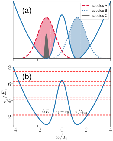
Figure 1: (a) Illustration of the initial ($t=0$) setup for the subsequent dynamics. The colored areas indicate the one-body densities of the different species. The majority species $A$ (red) and $B$ (blue) are displayed broader and with a larger maximum as compared to the impurity $C$ (grey), indicative of the corresponding particle-number ratios. The species $A$ and $C$ start in the left well ($x<0$), whereas the species $B$ is positioned in the right well ($x>0$). The interactions among identical bosons are weakly repulsive, whereas the inter-species interactions are switched off. (b) Spectrum of a single particle (impurity $C$) in a symmetric double-well potential, see Eq. 2.

II.1 Relaxation

The initial setup is illustrated in Fig. 1(a). The two majority species are prepared spatially separated on opposite sides of the double-well barrier in a self-trapped regime. The impurity can be localized in any of the two wells. Here, we choose the left well. Explicitly, we set $g_{\sigma\sigma}=0.2$ and overlay a species-dependent linear tilt $V_{\sigma}(x)=-d_{\sigma}\cdot x$ with $d_{A}=-d_{B}=d_{C}=0.5$ to energetically favor a particular side of the double-well, i. e., to account for the ‘loading’ process. Thus, species $A$ and $C$ experience a force to the left ($x<0$) and species $B$ to the right ($x>0$). The two majority components will act as site-dependent species embeddings for the impurity during propagation, but for now the inter-species interaction parameters are switched off, i. e., $g_{\sigma\bar{\sigma}}=0$. The corresponding Hamiltonian reads:

$$\mathcal{H}_{\rm{rlx}}=\sum_{\sigma}\mathcal{H}_{\sigma}+V_{\sigma}(x).$$ (5)

Our initial many-body state is the ground state of Eq. 5. It is obtained using ML-X by time propagating the non-interacting ground state of $\sum_{\sigma}\mathcal{H}^{(1)}_{\sigma}+V_{\sigma}(x)$ in imaginary time.

Note that the tilt $|d_{\sigma}|$ required to realize a self-trapped regime for a single-component condensate depends in a non-trivial way on the number of particles and the strength of intra-component interactions. For absent inter-component interactions, we have verified long-term localization of the two majority species in the initialized wells, which is a dynamical property we want also to maintain at finite majority-impurity interactions. That this must be the case is by far not obvious. What is rather more likely is that the self-trapping becomes destabilized or even destroyed by the impurity.

Alternatively to the species-dependent tilt potential $V_{\sigma}(x)$ for the initial state preparation one can set $g_{AB}$ to be repulsive such as to realize a phase-separated state between the majority species $A$ and $B$ and then impose a species-independent tilt. A sufficiently repulsive $g_{AB}$ can ensure that the species $A$ and $B$ stay localized at opposite wells, whereas the impurity $C$ relocates to a well favored by the chosen tilt.

II.2 Propagation

Given the initial state of a decoupled mixture ($g_{\sigma\bar{\sigma}}=0$) from Section II.1 at $t=0$, we instantaneously switch off the tilt to recreate the symmetric double well, i. e., $d_{\sigma}=0$. The dynamics is now governed by $\mathcal{H}_{t}$ from Eq. 4. The majority components become self-trapped owing to repulsive intra-species interactions, whereas the impurity undergoes tunneling. When the strength of majority-impurity interactions is at zero, the tunneling period $t_{\rm{tun}}=\pi/\Delta E$ for the impurity is determined by the energy gap $\Delta E$ between the two lowest eigenstates of Eq. 2 with $\sigma=C$, which for the selected double-well in Fig. 1(b) equals $t_{\rm{tun}}=90$ in harmonic units.

Now, we keep $g_{AB}(t)=0$ and control only the majority-impurity interactions $g_{AC}(t)$, $g_{BC}(t)$ such as to transfer the impurity to the opposite side of the double-well and freeze it there. To this end, we devise a simple time-dependent interaction scheme depicted in Fig. 2(a). It is a four-step procedure which we call the ‘transfer-pin-store-unpin’ protocol, which is characterized by the following durations: the fixed transfer time $t_{\rm{tr}}=t_{\rm{tun}}-1$, short (un)pin time $\Delta t=1$ and flexible storage time $t_{s}$.

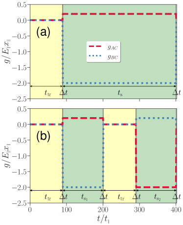
Figure 2: (a) Interaction protocol ‘transfer-pin-store-unpin’ characterized by a fixed transfer time $t_{\rm{tr}}=t_{\rm{tun}}-1$, which is determined by the tunneling time $t_{\rm{tun}}/t_{\parallel}=90$ according to the splitting of the lowest doublet in Fig. 1(b), flexible storage time $t_{s}$ and short (un)pinning times $\Delta t/t_{\parallel}=1$. At $t=0$, the impurity $C$ starts in the left well, occupied by species $A$. First, at $0<t<t_{\rm{tr}}$, it tunnels (yellow-shaded area) to the right well, occupied by species $B$. Then, at $0<t-t_{\rm{tr}}<\Delta t$, it is quickly pinned inside the right well by a linear ramp (narrow white-shaded area) of majority-impurity interactions with $g_{AC}\rightarrow g_{+}$ becoming repulsive and $g_{BC}\rightarrow g_{-}$ attractive. Note that in the figure the linear ramp resembles a quench due to very short times. Once pinned, at $0<t-t_{\rm{tr}}-\Delta t<t_{s}$, it is stored (green-shaded area) inside the right well, here $t_{s}/t_{\parallel}=310$. Finally, at $0<t-t_{\rm{tr}}-\Delta t-t_{s}<\Delta t$ it is unpinned by a linear ramp of interactions back to zero. (b) Interaction scheme ‘back-and-forth-transfer’ with variable storage times $t_{s_{1}}$ and $t_{s_{2}}$. At $t=0$, the impurity starts in the left well. First, we perform ‘transfer-pin-store-unpin’ to the right, similar to Fig. 2(a) except for a different storage time $t_{s_{1}}/t_{\parallel}=110$. Afterwards, we perform ‘transfer-pin-store-unpin’ to the left with a storage time $t_{s_{2}}/t_{\parallel}=110$. Note that for the back transfer the interactions have been inverted with $g_{AC}\rightarrow g_{-}$ becoming attractive and $g_{BC}\rightarrow g_{+}$ repulsive.

In the first step, the transfer, the majority-impurity interaction parameters are kept at zero, which lasts for $t_{\rm{tr}}$ (yellow-shaded area). During this time the impurity is allowed to freely tunnel. Once the tunneling to the opposite well is almost accomplished, the impurity features a large overlap with the component $B$. In the second step, the pin, we apply a linear ramp within a very short time window $\Delta t$ with $g_{AC}\rightarrow g_{+}$ becoming repulsive and $g_{BC}\rightarrow g_{-}$ attractive. The final values of interactions are $g_{+}=0.2$ and $g_{-}=-2$. Note that in Fig. 2(a), this step resembles a quench (very narrow white-shaded region). As a result, the impurity is captured by the component $B$ and is prevented from tunneling back. In the third step, the storage, we keep interactions constant for a flexible duration $t_{s}$ (green-shaded area). Finally, in the last step, the unpin, we very quickly ramp down the majority-impurity interactions linearly back to zero, within a very short time window $\Delta t$ (very narrow white-shaded area). From there, the impurity resumes its interrupted tunneling.

To transfer the impurity forth and back, we employ the protocol depicted in Fig. 2(b). Essentially, it applies ‘transfer-pin-store-unpin’ from Fig. 2(a) two times. First, we transfer the impurity to the right well and hold it there for $t_{s_{1}}=110$ with species $A$ being repulsive and $B$ attractive. Second, we transfer the impurity back to the original well and hold it there for $t_{s_{2}}=110$. As opposed to the first sequence, the species $A$ is now attractive and $B$ repulsive. Note that in the second sequence we use the same transfer period $t_{\rm{tr}}$, even though the state of the impurity is different from the one at $t=0$.

Let us note that, in principle, many other protocols could be imagined and applied. Indeed, we have explored several other strategies which, however, turned out to be much less successful. Nevertheless, we want to give a brief sketch of some alternative protocols and why they don’t work. First, we investigated much slower linear ramps by starting to change the majority-impurity interactions right at the start of transfer periods. As it turns out, already for a forward transfer this results in a fraction of the impurity density to be left behind, i. e., a sub-optimal transfer, whereas the majority component, interacting attractively with the impurity, sustains a sizable decay of self-trapping, thereby making it an unreliable container for the impurity during storage times. Second, we tried to quench the majority-impurity interactions at times immediately before and after the storage period, i. e., infinitely steep ramps. While the forward transfer was very promising, the subsequent back-transfer was less efficient as compared to the protocol from Fig. 2(b) in every aspect and, on top of that, extremely sensitive to the particular time of the impurity release.

III Method and Computational Approach

To obtain the initial state and to simulate the subsequent dynamics we need to solve the many-body Schrödinger equations for imaginary time $\partial_{\tau}\ket{\Psi(t)}=H_{\rm{rlx}}\ket{\Psi(t)}$ and for real time $i\partial_{t}\ket{\Psi(t)}=H_{t}\ket{\Psi(t)}$, respectively. One method is particularly well-tailored to this problem, especially in the context of multi-component systems of indistinguishable particles, the multi-layer multi-configuration time-dependent Hartree method for atomic mixtures [120, 121, 122], usually abbreviated as ML-MCDTHX but here, for short, we call it ML-X.

This ab-initio approach expands the many-body wave function in a finite orthonormal basis whose vectors are time-dependent and have a product form, properly symmetrized to account for the corresponding exchange symmetry of the identical particles. Both the basis and expansion coefficients are variationally optimized to span the relevant part of the full Hilbert space at each time step of the state evolution. This allows to reduce the total number of configurations as compared to a time-independent basis, which provides a great boost in convergence and makes larger system sizes numerically accessible. The multi-configuration ansatz takes interaction-induced inter-particle correlations into account, whereas the multi-layer structure introduces a hierarchy of Hilbert-space truncations by clustering together strongly correlated degrees of freedom (see below).

Our ansatz for a triple mixture has three layers of expansion. First, we formally group the spatial degrees of freedom of indistinguishable particles $\bigcup_{i}x^{\sigma}_{i}$ into three collective coordinates $q^{\sigma}$. Each $q^{\sigma}$ is then provided with a set of $S_{\sigma}$ time-dependent orthonormal species wave functions $\Psi_{i}^{\sigma}(q^{\sigma},t)$. In the first step, we expand our wave function $\ket{\Psi(t)}$ according to the following product form:

$$\ket{\Psi(t)}=\sum_{i=1}^{S_{A}}\sum_{j=1}^{S_{B}}\sum_{k=1}^{S_{C}}A_{ijk}(t)\ket{\Psi_{i}^{A}(t)}\otimes\ket{\Psi_{j}^{B}(t)}\otimes\ket{\Psi_{k}^{C}(t)},$$ (6)

where $A_{ijk}(t)\in\mathbb{C}$ are time-dependent expansion coefficients. This partitioning turns out to be particularly useful when correlations among species are considerably weaker compared to correlations among identical particles.

Next, since a species wave function characterizes identical bosons, each of them is expanded in terms of symmetrized and normalized product states $\ket{\vec{n}^{\sigma}(t)}$ (so-called permanents encoding that $n_{i}^{\sigma}$ particles occupy a time-dependent single-particle orbital $\varphi^{\sigma}_{i}(x,t)$):

$$\ket{\Psi_{i}^{\sigma}(t)}=\sum_{\vec{n}^{\sigma}|N_{\sigma}}C_{i,\vec{n}^{\sigma}}(t)\ket{\vec{n}^{\sigma}(t)},$$ (7)

where $C_{i,\vec{n}^{\sigma}}(t)\in\mathbb{C}$ are time-dependent expansion coefficients, $\vec{n}^{\sigma}|N_{\sigma}$ restricts the Fock space to configurations with a fixed number of particles $\sum_{i}n_{i}^{\sigma}=N_{\sigma}$, further truncated to $s_{\sigma}$ single-particle orbitals which can be occupied. The Fock space dimension is thus given by a binomial coefficient $\binom{N_{\sigma}+s_{\sigma}-1}{N_{\sigma}}$.

Finally, applying any of the, in case of analyticity, equivalent time-dependent variational principles [128] leads to a set of coupled time-differential equations for $A_{ijk}(t)$, $C_{i,\vec{n}^{\sigma}}(t)$ and $\varphi^{\sigma}_{i}(x,t)$. The single-particle functions are represented in a time-independent basis of $s_{g}$ spatially-localized functions $\chi_{\alpha}(x_{\beta})=\delta_{\alpha,\beta}$ (grid DVR) [129]:

$$\ket{\varphi_{i}^{\sigma}(t)}=\sum_{\alpha}d_{i;\alpha}^{\sigma}(t)\ket{\chi_{\alpha}},$$ (8)

where $d_{i;\alpha}^{\sigma}(t)\in\mathbb{C}$ are time-dependent expansion coefficients. Note that our grid does not depend on the species label $\sigma$.

The parameter $s_{g}$ defines the number of grid points to resolve spatial variations of time-evolving single particle functions. To fulfill this requirement, we choose an equally spaced grid with $s_{g}=300$ spanning an interval $\left[x_{\rm{min}},x_{\rm{max}}\right]=\left[-7,7\right]$. The parameter $S_{\sigma}$ truncates correlations between distinct particles, the so-called inter-species correlations or entanglement. For selected physical parameters we find $S_{A}=S_{B}=S_{C}-1=3$ to be suitable to faithfully capture the dynamical build-up of entanglement. The parameter $s_{\sigma}$ truncates correlations among identical particles, the so-called intra-species correlations or fragmentation. We find $s_{\sigma}=4$ to be sufficient to account for majority depletion, which is primarily caused by majority-component interactions of strength $g_{\sigma\sigma}$. Note that $S_{\sigma}\leq\binom{N_{\sigma}+s_{\sigma}-1}{N_{\sigma}}$. Simulations performed with the above choice of numerical parameters $S_{\sigma}$, $s_{\sigma}$ and $s_{g}$ will be referred to as ML-X simulations. Additionally, let us mention two kinds of approximate solutions. Setting $S_{\sigma}=1$ neglects entanglement among species and is called a species-mean-field (SMF) ansatz. Setting $s_{\sigma}=1$, implying also that $S_{\sigma}=1$, neglects all types of correlations and is known as a mean-field ansatz or coupled Gross-Pitaevskii equations (cGPE).

IV Results, Analysis and Discussion

IV.1 A single transfer

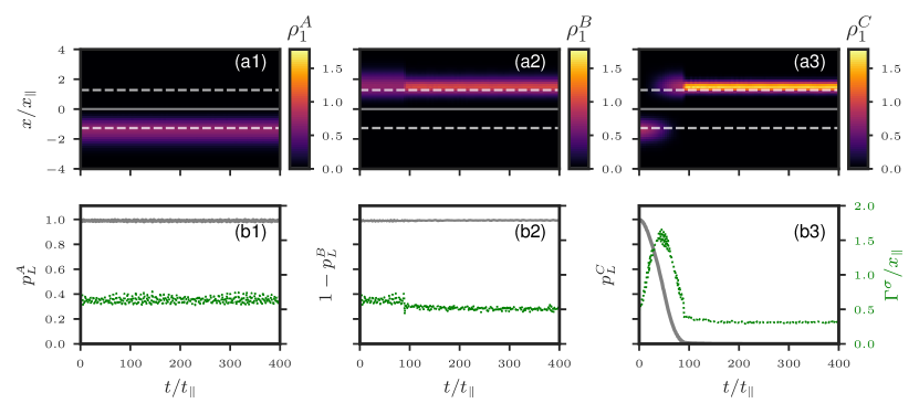
Figure 3: Time-evolution of several observables after quenching the tilt of the external potential to zero and, subsequently, following the majority-impurity interaction scheme as depicted in Fig. 2(a). (a1)-(a3): The one-particle density distribution $\rho_{1}^{\sigma}(x,t)$ of species $\sigma$: $A(B)$ denotes a self-trapped majority component while $C$ stands for the impurity. The gray solid line at $x=0$ indicates the position of the double-well barrier and the gray dashed lines at $x/x_{\parallel}\approx\pm 1.27$ the position of the double-well minima. (b1)-(b3): the integrated probability $p_{L}^{\sigma}(t)$ or 1-$p_{L}^{\sigma}(t)$ (gray solid line) to find a particle of component $\sigma$ on the left or right side of the double-well potential, respectively, and the standard deviation of the density distribution $\Gamma^{\sigma}(t)$ (green dotted line).

First, we apply the interaction protocol from Fig. 2(a). The goal of this scheme is to realize a smooth transfer of an initially localized impurity to the opposite well and, subsequently, to store it inside that well for a specified time period $t_{s}$ while maintaining the shape of the underlying density distribution to resemble a Gaussian of a similar width as the initial wave-packet. The majority components are required to remain self-trapped and well-localized during the entire protocol. It goes without saying that such a transfer where the impurity is embedded into separate background majority species on the left and on the right well is not only a physically very different situation from the transfer of an isolated single atom but is also much more difficult to achieve.

In Fig. 3 (a1)-(a3) we show the time-evolution of one-body densities $\rho_{1}^{\sigma}(x,t)$ for each species. In Fig. 3 (b1)-(b3) we present the corresponding integrated quantities: i) $p^{\sigma}_{L}(t)=\int_{-\infty}^{0}dx\;\rho_{1}^{\sigma}(x,t)=1-p^{\sigma}_{R}(t)$, which indicates the probability for a particle of species $\sigma$ to be located on the left side w. r. t. the double-well barrier, and ii) $\Gamma^{\sigma}(t)=\sqrt{\int dx\;x^{2}\rho_{1}^{\sigma}(x,t)-[\int dx\;x\rho_{1}^{\sigma}(x,t)]^{2}}$ which is the standard deviation of the corresponding density distribution.

The majority component $A$, see Fig. 3 (a1) and (b1), initialized in the left well, the same as the impurity, is barely affected by the protocol. During the transfer period $t_{\rm{tr}}$, when the majority-impurity interactions are at zero, the observed dynamics is a result of the initialization procedure, namely quenching the tilt of the external potential to zero triggers low-amplitude high-frequency dipole-like oscillations in the initial density distribution. Note that this dynamics does not destroy the self-trapping regime of the majority component for long times. By the time the majority-impurity interactions are switched on, the impurity has tunneled from the left to the right well and the component $A$, interacting now repulsively with the impurity, has no sizable overlap with it during the storage time $t_{s}$ to be noticeably affected. Thus, the species $A$ remains self-trapped and localized in the left well the whole time as desired. In particular, it acts as a ‘material barrier’ for the impurity making it energetically unfavorable for the impurity to tunnel back to its initial left well.

The majority component $B$, see Fig. 3 (a2) and (b2), initialized in the right well exhibits a mirror dynamics compared to component $A$ during the transfer time $t_{\rm{tr}}$. During the storage period $t_{s}$, when the interactions between the component $B$ and the impurity become attractive and there is a large overlap between them, the component $B$ becomes slightly compressed while density fluctuations get reduced. Importantly, the species $B$ also remains self-trapped and well-localized. On top of that, it acts as a ‘container’ for the impurity preventing it from dispersing within the storage well.

The impurity $C$, see Fig. 3 (a3) and (b3), first undergoes a free tunneling process during the transfer time $t_{\rm{tr}}$: the density distribution delocalizes and finally localizes again at the opposite well. Then, the impurity becomes quickly pinned accompanied by an additional compression of the density. During the storage time $t_{s}$ it remains highly localized and features only minor fluctuations of the mean position and width reminiscent of sloshing oscillations.

IV.2 Back-and-forth transfer

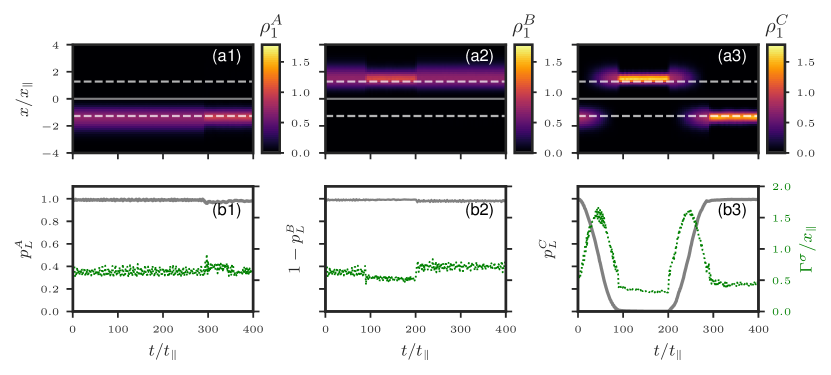
Figure 4: Time-evolution of several observables after quenching the tilt of the external potential to zero and, subsequently, following the majority-impurity interaction scheme as depicted in Fig. 2(b). (a1)-(a3): The one-particle density distribution $\rho_{1}^{\sigma}(x,t)$ of species $\sigma$: $A(B)$ denotes a self-trapped majority component while $C$ stands for the impurity. The gray solid line at $x=0$ indicates the position of the double-well barrier and the gray dashed lines at $x/x_{\parallel}\approx\pm 1.27$ the position of the double-well minima. (b1)-(b3): the integrated probability $p_{L}^{\sigma}(t)$ or 1-$p_{L}^{\sigma}(t)$ (gray solid line) to find a particle of component $\sigma$ on the left or right side of the double-well potential, respectively, and the standard deviation of the density distribution $\Gamma^{\sigma}(t)$ (green dotted line).

Next, we analyze the interaction protocol depicted in Fig. 2(b). The goal of this scheme is to demonstrate the reverse process, i. e., that the impurity can be just as smoothly transported back and pinned at the left well, by applying a ‘mirror’ protocol starting at $t=t_{\rm{tr}}+2\Delta t+t_{s_{1}}$. This is by far not obvious, since the many-body wave function has become species-entangled (see later) as compared to the initial species-disentangled state at zero inter-species interactions. Importantly, we find (see Section IV.4) that the storage performance of the second sequence (at the left well) is not sizably affected by the storage time $t_{s_{1}}$ of the first sequence (at the right well), which is yet another benefit of the protocol from Fig. 2(b) in addition to its simplicity.

The corresponding observables are shown in Fig. 4. The majority component $A$, see Fig. 4 (a1) and (b1), is visibly affected by the interaction protocol only when it becomes attractive to the impurity, namely during the second transfer-and-storage sequence. At this time interval ($t>291$), it sustains very minor density losses to the opposite well, which can seen by an overall decrease of $p^{A}_{L}$ (gray solid line), but remains otherwise well-localized as indicated by only minor fluctuations in $\Gamma^{A}$ (green dotted line). The majority component $B$, see Fig. 4 (a2) and (b2), is also visibly affected by the interaction protocol only when it is attractive to the impurity, namely during the first transfer-and-storage sequence. After the interactions have been ramped down, the density sustains slight losses to the opposite well, but otherwise restores (to a large extent) its initial shape from $t=0$. Overall, both majority components remain self-trapped and localized as intended. The impurity $C$, see Fig. 4 (a3) and (b3), features slightly higher density losses to the opposite well during the second storage time and is on average less compressed. Nevertheless, the second transfer-and-storage sequence is just as smooth and stable.

Considering that a back-and-forth transfer includes a single transfer as its first sequence, we concentrate on the former from now on.

IV.3 Entanglement measures and analysis

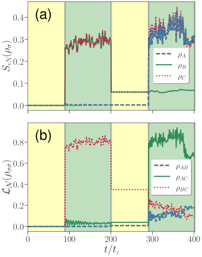
Figure 5: Time-evolution of entanglement measures after quenching the tilt of the external potential to zero and, subsequently, following the majority-impurity interaction scheme as depicted in Fig. 2(b). (a): the von-Neumann entropy $S_{\rm{vN}}(\rho_{\sigma})$, see Eq. 9, of a reduced single-species density $\rho_{\sigma}$. (b): the logarithmic negativity $\mathcal{L}_{\mathcal{N}}(\rho_{\sigma\bar{\sigma}})$, see Eq. 12, for a two-component subsystem described by a mixed state $\rho_{\sigma\bar{\sigma}}$ with $\sigma\neq\bar{\sigma}$.

We proceed by analyzing the build-up of entanglement for the back-and-forth transfer based on the protocol provided in Fig. 2(b). To this end, we employ two measures: the von-Neumann entropy $S_{\rm{vN}}$ and the logarithmic negativity $\mathcal{L}_{\mathcal{N}}$.

The von-Neumann entropy $S_{\rm{vN}}$ characterizes entanglement of a bipartite system. Our system, however, is tripartite. To render it bipartite, we partition it into a single-component and a double-component subsystems. This gives us three measures defined as follows:

$$S_{\rm{vN}}(\rho_{\sigma})=-\sum_{j}\lambda_{j}^{\sigma}\log(\lambda_{j}^{\sigma}),$$ (9)

$$\rho_{\sigma}=\operatorname{Tr}_{\sigma^{\prime}\neq\sigma}[\rho]=\sum_{j}\lambda_{j}^{\sigma}\ket{\Phi^{\sigma}_{j}}\bra{\Phi^{\sigma}_{j}},$$ (10)

where $\rho_{\sigma}$ is the reduced density matrix of a component $\sigma$ obtained from a pure many-body state $\rho$ by tracing out all particles from other components $\sigma^{\prime}\neq\sigma$. Here, it is represented in terms of natural orbitals $\ket{\Phi^{\sigma}_{j}}$ (eigenvectors) and natural populations $\lambda_{j}^{\sigma}$ (eigenvalues) satisfying $\sum_{j}\lambda_{j}^{\sigma}=1$ and $\lambda_{1}>\dots>\lambda_{S_{\sigma}}$. In the absence of entanglement $\lambda_{1}=1$ and $S_{\rm{vN}}=0$ vanishes. For a maximally entangled state all natural populations are the same, i. e., $\lambda_{j}=1/S_{\sigma}\;\forall j$ (see Section III), which gives $S_{\rm{vN}}=\log{S_{\sigma}}$.

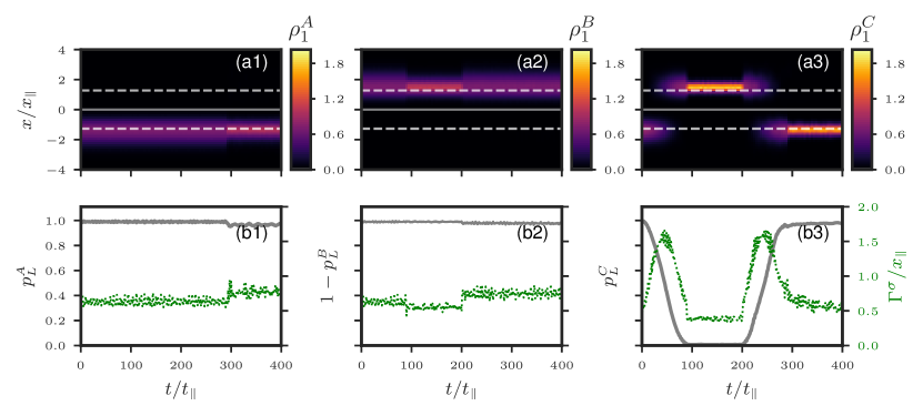
Figure 6: Time-evolution of several observables after quenching the tilt of the external potential to zero and, subsequently, following the majority-impurity interaction scheme as depicted in Fig. 2(b). The physical and numerical parameters are the same as Fig. 4 except here we neglect the entanglement in the ML-X ansatz ($S_{\sigma}=1$) for the many-body wave function, see Section III. (a1-a3): The one-particle density distribution $\rho_{1}^{\sigma}(x,t)$ of species $\sigma$: $A(B)$ denotes a self-trapped majority component while $C$ stands for the impurity. The gray solid line at $x=0$ indicates the position of the double-well barrier and the gray dashed lines at $x/x_{\parallel}\approx\pm 1.27$ the position of the double-well minima. (b1-b3): the integrated probability $p_{L}^{\sigma}(t)$ or 1-$p_{L}^{\sigma}(t)$ (gray solid line) to find a particle of component $\sigma$ on the left or right side of the double-well potential, respectively, and the standard deviation of the density distribution $\Gamma^{\sigma}(t)$ (green dotted line).

The von-Neumann entropy is depicted in Fig. 5(a). Keep in mind that it tells us whether a single component is entangled with a pair of other two components. In particular, it lacks the ability to resolve entanglement between any specific two components of a tripartite system. During the first transfer period, which is free of inter-component interactions, there is no entanglement as expected. After the ramp-up, at $t=90$, the components $B$ and $C$ have (individually) accumulated a sizable and comparable amount of entanglement, whereas the component $A$ is not (notably) entangled. This is in accordance with our expectations: during the ramp-up $B$ and $C$ feature a large overlap with each other and almost no overlap with $A$. Thus, it might be reasonable to assume a product state between subsystems $A$ and $B-C$. During the subsequent storage time, when interactions are kept fixed, we observe fluctuations of the entropy in components $B$ and $C$. After the ramp-down, at $t=200$, the entropy of $B$ and $C$ has dropped considerably and, for the next transfer period at zero majority-impurity interactions, becomes frozen. The component $A$ is still not noticeably affected for the same reasons as before.

At the start of the second ramp-up at $t=290$, the relations become alternated: $C$ has returned to the left well occupied by $A$, such that now $A$ and $C$ become (individually) strongly entangled. During the subsequent storage time, the corresponding entropies undergo larger-amplitude fluctuations as opposed to $B$ and $C$ in the first storage period. In addition, they do not exactly match each other. Regarding the component $B$, it preserves the value of entropy accumulated after the first storage-and-transfer sequence and features only minor fluctuations during the second storage period.

Thus, the evolution of the von-Neumann entropy follows a particular pattern. It remains frozen at non-interacting transfer times. For overlapping components it builds up when interactions are ramped up, and abruptly decays but stays finite when interactions are ramped down. Moreover, it features large-amplitude fluctuations during storage times. To resolve to which extent one single component is entangled with another single component, we require a different measure.

The logarithmic negativity $\mathcal{L}_{\mathcal{N}}$ quantifies pair-wise entanglement between two distinct components $\sigma$ and $\bar{\sigma}$, which are described by a mixed state $\rho_{\sigma\bar{\sigma}}$. The latter is obtained from a pure many-body state $\rho$ by tracing out all particles from the third component $\sigma^{\prime}\notin\left\{\sigma,\bar{\sigma}\right\}$:

$$\rho_{\sigma\bar{\sigma}}=\operatorname{Tr}_{\sigma^{\prime}\notin\left\{\sigma,\bar{\sigma}\right\}}[\rho]=\sum_{i,j,k,l}b_{ijkl}\ket{\Psi^{\sigma}_{i},\Psi^{\bar{\sigma}}_{j}}\bra{\Psi^{\sigma}_{k},\Psi^{\bar{\sigma}}_{l}},$$ (11)

here represented in terms of species orbitals $\ket{\Psi^{\sigma}_{i}}$ of the ML-X expansion from Eqs. 6 and 7. The logarithmic negativity $\mathcal{L}_{\mathcal{N}}$ depends on the partial transpose $\rho_{\sigma\bar{\sigma}}^{T_{\sigma}}$ in the following way:

$$\mathcal{L}_{\mathcal{N}}(\rho_{\sigma\bar{\sigma}})=\log_{2}(|\rho_{\sigma\bar{\sigma}}^{T_{\sigma}}|_{1})=\log_{2}(1+2\mathcal{N}),$$ (12)

$$\rho_{\sigma\bar{\sigma}}^{T_{\sigma}}=\sum_{i,j}b_{kjil}\ket{\Psi^{\sigma}_{i},\Psi^{\bar{\sigma}}_{j}}\bra{\Psi^{\sigma}_{k},\Psi^{\bar{\sigma}}_{l}}=(\rho_{\sigma\bar{\sigma}}^{T_{\bar{\sigma}}})^{T},$$ (13)

with $|\rho|_{1}=\operatorname{Tr}\left\{\sqrt{\rho^{\dagger}\rho}\right\}$ the trace norm and $\mathcal{N}=\sum_{i}|\mu_{i}|$ the negativity, which is the sum of negative eigenvalues $\mu_{i}<0$ of $\rho_{\sigma\bar{\sigma}}^{T_{\sigma}}$. When there is no entanglement between components $\sigma$ and $\bar{\sigma}$, $\rho_{\sigma\bar{\sigma}}^{T_{\sigma}}$ is positive semi-definite and $\mathcal{L}_{\mathcal{N}}=0$ vanishes. Otherwise, it is positive with larger values indicating a stronger entanglement.

The logarithmic negativity is depicted in Fig. 5(b). For the first transfer-and-storage sequence ($t<200$), the high values of entropy for the components $B$ and $C$ can be now indeed attributed to them being pairwise entangled with each other. The entanglement between $A$ and $C$ (green solid line) becomes also more apparent, though it is still an order of magnitude less than between $B$ and $C$ (red dotted line). There is no entanglement between $A$ and $B$ (blue dashed line) as expected.

For the second transfer-and-storage sequence ($t>200$) the distribution of entanglement is less obvious. Remarkably, during the ramp-up we observe a gradual build-up of entanglement between $A$ and $B$. As they are non-interacting and barely overlap, it must be mediated by the tunneling impurity. At the same time, the entanglement between $B$ and $C$ decreases by a similar amount, which is in accordance with a (roughly) constant entropy of $B$ mentioned before. The logarithmic negativity between $A$ and $C$ behaves similarly to the evolution of individual entropies of $A$ or $C$ in Fig. 5(a) at $t>291$. Thus, the logarithmic negativity provides complementary insights into the build-up of entanglement in a tripartite system. To some extent, the entropy of a component $\sigma$ is proportional to a sum of logarithmic negativities involving that component.

Given that the inter-species entanglement is quite sizable during the dynamics, one might ask what impact it has on the ongoing dynamics, in particular the impurity motion. To this end, in Fig. 6 we show the previously analyzed observables for the back-and-forth transfer assuming now a SMF expansion ($S_{\sigma}=1$) for the many-body wave function, as introduced in Section III. We remind that this ansatz assumes a single product state in Eq. 6, thus ignoring entirely any inter-species correlations. Apparently, the majority components are not visibly affected when compared to Fig. 4, whereas the impurity seems to be destabilized by the absence of inter-species correlations, featuring larger fluctuations on the density width, see Fig. 6(b3). Thus, the build-up of entanglement contributes in a non-trivial way to a robust transfer and storage of the impurity particle.

Furthermore, a mean-field ansatz ($s_{\sigma}=1$) displays a similar dynamics to Fig. 6 (see Appendix). Initially, the majority components are almost condensed. In the course of the dynamics, they experience only a slight fragmentation ($\sim 3\%$), which explains the strong similarity between uncorrelated and correlated results. In this spirit, we have done mean-field simulations for $N_{A}=N_{B}=20$ with $g_{A}=g_{B}=0.1$ and $N_{A}=N_{B}=50$ with $g_{A}=g_{B}=0.04$ (see Appendix). Again, we observed a very similar dynamics to Fig. 6. Among the differences, we noticed that during storage the width of the impurity density and its fluctuations increase with an increasing number of particles, which has a negative impact on the storage performance. However, it might be that correlations will stabilize the impurity, though we cannot verify it here numerically given the increased computational complexity.

IV.4 Effective potential analysis

While applying a variational approach, such as ML-X, to solve the time-dependent Schrödinger equation turns out to be efficient in terms of sparsity of the wave function representation, it often comes at the cost of reduced interpretability. Thus, the variationally optimal single-particle orbitals can be rarely assigned as eigenstates of a single particle in some external potential. However, having such a picture can be often helpful to understand some dynamical processes. One such example is a mean-field picture where interacting particles experience the averaged spatial distribution of all other particles as an effective external potential and behave accordingly.

Here, we want to provide a similar viewpoint on the dynamics of the impurity. To this end, we are going to decompose the corresponding (one-body) density operator $\rho_{C}\equiv\rho_{1}^{C}$, see Eq. 10, into projections $p_{j}\geq 0$ on single-particle basis states $\left\{\ket{\phi_{j}}\right\}$, which gives us a distribution of occupation probabilities over these states. As our projection basis we choose eigenstates of a time-dependent effective Hamiltonian:

$$(\mathcal{H}^{(1)}_{\sigma}+V_{\rm{ind}}^{\sigma}(t))\ket{\phi^{\sigma}_{j}(t)}=\epsilon^{\sigma}_{j}(t)\ket{\phi^{\sigma}_{j}(t)},$$ (14)

$$V_{\rm{ind}}^{\sigma}(x,t)=\sum_{\sigma^{\prime}\neq\sigma}N_{\sigma^{\prime}}g_{\sigma\sigma^{\prime}}(t)\rho_{1}^{\sigma^{\prime}}(x,t),$$ (15)

$$p_{j}^{\sigma}(t)=\braket{\phi^{\sigma}_{j}(t)}{\rho_{1}^{\sigma}(t)}{\phi^{\sigma}_{j}(t)},$$ (16)

where $\rho_{1}^{\sigma}=\operatorname{Tr}_{N_{\sigma}-1}[\rho_{\sigma}]$ is obtained from $\rho_{\sigma}$, see Eq. 10, by tracing out all $\sigma$ particles except one, $\epsilon^{\sigma}_{j}$ the eigenenergy of $\ket{\phi^{\sigma}_{j}}$ and $g_{\sigma\sigma^{\prime}}(t)$ evolving according to the back-and-forth interaction protocol from Fig. 2(b). We note that $\rho_{1}^{\sigma}(t)$ is obtained from a correlated many-body state $\rho(t)=\ket{\Psi(t)}\bra{\Psi(t)}$ as defined in Section III with $S_{A}=S_{B}=S_{C}-1=3$ and $s_{\sigma}=4$.

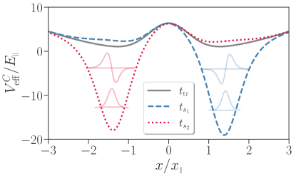
Figure 7: Effective potential $V_{\rm{eff}}^{C}(t)=V_{\rm{dw}}+V_{\rm{ind}}^{C}(t)$ for the impurity $C$ during the back-and-forth interaction protocol from Fig. 2(b) averaged over selected time intervals: transfer period $t_{\rm{tr}}$ (gray solid line), first storage period $t_{s_{1}}$ (blue dashed line) and second storage period $t_{s_{2}}$ (red dotted line). The potential is a superposition of an external (static) double-well trap $V_{\rm{dw}}$ from Fig. 1(b) with a (time-dependent) material barrier and well $V_{\rm{ind}}^{C}(t)$ from Eq. 15 which is created by the interchangeably repulsive and attractive majority components. The solid red and blue curves indicate the two lowest-energy eigenstates of the corresponding potentials at designated eigenenergies.

The induced potential $V_{\rm{ind}}^{\sigma}$ in Eq. 15 is a sum over (time-dependent) one-body densities of the two majority components, each amplified by the number of particles and further modulated by the time-dependent majority-impurity interaction parameter. We already know from Section IV.2 that in the course of the dynamics the majority components remain self-trapped in the initially prepared well. Moreover, they take a Gaussian-like shape localized at the minimum of the corresponding well with only small-amplitude fluctuations around that minimum. Thus, during storage times the repulsive component represents a potential barrier for the impurity, thereby decreasing the depth of the corresponding external well, whereas the attractive component acts as a potential well, i. e., it increases the depth of the corresponding external well even further. As a result, we get an asymmetric double-well potential, see Fig. 7. Even though this effective potential picture for the impurity is formally related to a species-mean-field (non-entangled) ansatz for a triple mixture, we emphasize that our many-body state $\rho$ and the corresponding derived quantities $\rho_{1}^{\sigma}$ include inter-species correlations.

In Fig. 8 we show the evolution of probabilities $p_{j}^{C}(t)$ from Eq. 16 for the impurity to occupy the eigenstates $\left\{\ket{\phi_{j}^{C}(t)}\right\}$ of the Hamiltonian Eq. 14 and the corresponding instantaneous eigenenergies $\epsilon^{\sigma}_{j}(t)$. Initially, the state of the impurity is an almost equal superposition of the two lowest (quasi-degenerate) eigenstates of the symmetric double-well potential, see also Fig. 1(b). Thus, it tunnels. After the first ramp-up of interactions at $t=90$, the right well becomes energetically more favorable, and we get an asymmetric double-well, see Fig. 7 (blue dashed curve). The impurity still occupies the two lowest eigenstates though the weights of occupations are now largely shifted in favor of the ground state, which is now a Gaussian localized at the right well. A slight contribution of the first excited state explains the high-frequency low-amplitude dipole motion, i. e., the left-to-right sloshing, of the impurity density inside the right well during the storage time. The low-amplitude fluctuations of occupation probabilities are due to interaction with the majority component $B$, which undergoes a dipole motion inside the right well excited at $t=0$ by the instantaneous removal of the external tilt potential.

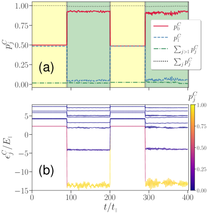
Figure 8: Projectors on instantaneous single-particle eigenstates $p_{j}^{C}$ (a) and instantaneous eigenenergies $\epsilon_{j}^{C}$ (b) of the time-dependent effective Hamiltonian from Eq. 14 for the impurity C, which includes time-dependent induced potentials (see Eq. 15) created by the majority components $A$ and $B$. In (b), each eigenenergy $\epsilon_{j}^{C}$ is color-coded with its occupation probability $p_{j}^{C}$ extracted from (a).

Once interactions have been ramped down at $t=201$, we recover the symmetric double-well potential and (to a good approximation) the same state composition (in terms of amplitudes) as before the storage sequence. The impurity resumes the tunneling motion with the same oscillation frequency. The aforementioned sloshing motion of the impurity impacts the phases of contributing double-well states and thus also the time it takes to tunnel back. However, given that the amplitude of sloshing is rather small, we do not encounter major differences on the transfer time $t_{\rm{tr}}$ upon changing the storage time $t_{s}$. In other words, we can release the impurity at any point in time during the storage sequence. This has been verified numerically for a random sample of storage times taken in the interval $t_{s_{1}}\in[150,300]$.

Regarding the second transfer-and-storage sequence, we observe the same patterns except for fluctuations during the storage time becoming larger. This might be caused by the minor decay of self-trapping in the majority components and related density losses to the opposite well, see Fig. 4.

V Conclusions and Outlook

We have investigated the possibilities for a controlled impurity tunneling dynamics in a double-well containing a mixture of three distinct species. Building upon insights from the literature, we prepared two bosonic species of ten atoms each in a self-trapped configuration on opposite sides of the double-well barrier to act as a background for the embedded impurity. By a suitable manipulation of majority-impurity interactions we realized a smooth transport and demonstrated a robust storage of the impurity. The study was conducted employing the multi-layer multi-configuration time-dependent Hartree method for bosonic mixtures.

The protocol consists of a sequence of quick ramps of interaction parameters and does not require any fine tuning. To initiate trapping, one majority component is made weakly repulsive and the other strongly attractive, depending on the storage well. To initiate transport, interactions are switched off. The transfer time is determined by the double-well geometry and the ramp time needs to be much smaller than the (lowest-band) tunneling time and the storage time is very flexible (within simulated times). The protocol is similar in spirit to the pinning procedure in quantum gas microscopy where one freezes the position of particles by an instantaneous ramp of the lattice depth.

The impurity undergoes a low-frequency large-amplitude dipole oscillation between wells during transfer times and high-frequency small-amplitude dipole motion inside a single well during storage times. The majority components remain self-trapped and perform high-frequency low-amplitude sloshing motion around the double-well minima. We have analyzed the role of entanglement in terms of the von-Neumann entropy and the logarithmic negativity. Our initial state is not entangled. We find that during ramps the impurity becomes strongly correlated with the attractive majority component. Subsequently, the accumulated entanglement undergoes low-amplitude modulations during storage times. After a ramp-down, the entanglement becomes greatly reduced but remains finite. Interestingly, during the back-and-forth transfer, we evidenced a build-up of entanglement between the two majority components, even though they do not interact and barely overlap. Apparently, the impurity mediates correlations between spatially-separated majority components. Furthermore, we compared the correlated many-body dynamics to a species-mean-field dynamics, which ignores all entanglement effects. Even though we find a good overall agreement between observables, there were also sizable discrepancies. The entanglement has a stabilizing impact on the dynamics by reducing the amplitude of density fluctuations during transfer and storage times.

Finally, we applied an effective potential picture to describe the impurity motion as an independent particle evolving in a time-dependent potential, which alternates between symmetric and asymmetric double wells. This potential includes a static double-well and time-dependent mean-fields produced by the majority particles. The dynamics is well captured by the two lowest eigenstates of this effective potential. During transfer times the two eigenstates contribute equally, and during storage times the ground state dominates with minor fluctuations caused by oscillations of the mean fields.

Even though the current protocol demonstrates already some very good results, the underlying minor imperfections might be amplified as the number of transfer-and-storage cycles is increased. The partial decay of self-trapping in the majority species might be compensated by introducing repulsive interactions among majority components or by changing the strength of intraspecies interactions. In addition, the entanglement between components was observed to gradually increase with every transfer-and-storage sequence, which might become a limiting factor requiring a disentangling procedure. The latter can be realized by optimizing the ramp times and/or the strength of majority-impurity interactions individually for each transfer-and-storage cycle.

Considering that the impurity can be switched between two configurations, left $\ket{L}$ and right $\ket{R}$, the setup might serve as a basic building block of a quantum circuit. However, the protocol needs to be modified to also include arbitrary superposition states, i. e., $c_{L}\ket{L}+c_{R}\ket{R}$. To this end, as opposed to the current protocol, we would adapt the transfer times accordingly and introduce purely attractive majority-impurity couplings to confine each density fraction independently during storage times. Finally, to build a quantum circuit, one needs to arrange such qubits in a lattice geometry, e. g., by using arrays of optical tweezers. Another interesting topic deserving a thorough investigation is the gradual build-up of entanglement between non-interacting majority components, mediated through the impurity.

Appendix A The impact of majority-impurity interaction values.

Regarding the choice of protocol parameters $g_{\pm}$ for the forward transfer, we have studied several combinations of parameter values $(g_{+},g_{-})$ and judged on their performance by evaluating the time-averaged probability $\tilde{p}_{\mathrm{R}}^{C}=\frac{1}{t_{s}}\int_{0}^{t_{s}}dt\;p_{\mathrm{R}}^{C}(t-t_{\rm{tr}}-\Delta t)$ for the impurity to be successfully stored in the right well during the storage time. The results can be seen in Table 1. All pairs of considered interaction values perform quite well with only minor differences among them. As we were not able to recognize any conclusive trends, we have chosen $g_{-}=-2$ and $g_{+}=0.2$ among best performing pairs.

$\tilde{p}_{\mathrm{R}}^{C}$		$g_{+}$
		$0.1$	$0.2$	$0.5$	$0.7$
$g_{-}$	$-1.5$	$0.995$	$0.997$	$0.998$	$0.998$
	$-2.0$	$0.998$	$0.998$	$0.998$	$0.998$
	$-5.0$	$0.997$	$0.997$	$0.996$	$0.996$

Table 1: Probability $\tilde{p}_{\mathrm{R}}^{C}$ to find the impurity on the right side of the symmetric double-well potential during the storage time $t_{s}$ following the interaction scheme from Fig. 2(a) for multiple choices of protocol parameters $g_{+}$ and $g_{-}$.

In a similar way, to select parameters $g_{\pm}$ for the forward and backward transfers, we evaluated the transfer performance by calculating the time-averaged probability $\tilde{p}_{\mathrm{L}}^{C}=\frac{1}{t_{s_{2}}}\int_{0}^{t_{s_{2}}}dt\;p_{\mathrm{L}}^{C}(t-2t_{\rm{tr}}-3\Delta t-t_{s_{1}})$ for the impurity to be successfully pinned at the left well during the second storage sequence. The results can be seen in Table 2. As compared to Table 1 the storage performance has slightly decreased over all parameter pairs, especially at strong attractions $g_{-}=-5$. Our former choice $g_{-}=-2$ and $g_{+}=0.2$ performs comparatively well.

$\tilde{p}_{\mathrm{L}}^{C}$		$g_{+}$
		$0.1$	$0.2$	$0.5$	$0.7$
$g_{-}$	$-1.5$	$0.993$	$0.994$	$0.993$	$0.992$
	$-2.0$	$0.990$	$0.992$	$0.990$	$0.992$
	$-5.0$	$0.987$	$0.986$	$0.982$	$0.983$

Table 2: Probability $\tilde{p}_{\mathrm{L}}^{C}$ to find the impurity on the left side of the symmetric double-well potential during the storage time $t_{s_{2}}$ following the interaction scheme from Fig. 2(b) for multiple choices of protocol parameters $g_{+}$ and $g_{-}$.

Appendix B The impact of particle-number imbalance using a mean-field ansatz.

Initially, the majority components are almost condensed. In the course of the dynamics the degree of fragmentation gradually increases, though the condensed fraction does never drop below $97\%$. In this spirit, a mean-field ansatz might provide a very good qualitative description of the ongoing dynamics. Indeed, Fig. 9 bears a strong similarity to ML-X simulations from Fig. 4. There are only slight differences as compared to a species-mean-field ansatz from Fig. 6.

These observations motivate us to employ a mean-field ansatz to explore the dependence of our protocol on the number of particles in majority components. In order to maintain the self-trapping regime, we keep $N_{\sigma}g_{\sigma\sigma}$ constant. In Fig. 10 we show the forth-and-back transfer for $N_{A}=N_{B}=20$ and $g_{A}=g_{B}=0.1$ and in Fig. 11 for $N_{A}=N_{B}=50$ and $g_{A}=g_{B}=0.04$. Qualitatively, the dynamics is similar to Fig. 9. Among differences, the width of the impurity density and its fluctuations increase with increasing number of particles. This decreases the storage performance. Nevertheless, the inter-species correlations might stabilize the impurity, though we cannot verify it with ML-X owing to the exponential scaling of the Hilbert space dimension with the number of particles.

Figure 9: Same as Fig. 6 except here we employ a mean-field ansatz. $N_{A}=N_{B}=10$ and $g_{A}=g_{B}=0.2$.

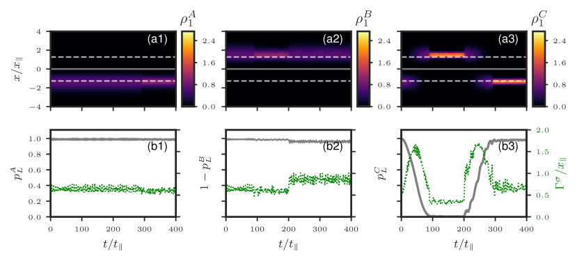
Figure 10: Same as Fig. 6 except here we employ a mean-field ansatz. $N_{A}=N_{B}=20$ and $g_{A}=g_{B}=0.1$.

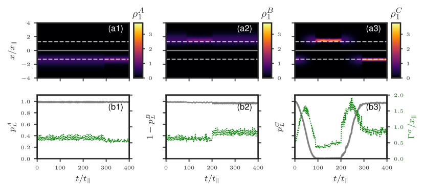
Figure 11: Same as Fig. 6 except here we employ a mean-field ansatz. $N_{A}=N_{B}=50$ and $g_{A}=g_{B}=0.04$.

References

- Kawaura et al. [2000] H. Kawaura, T. Sakamoto, and T. Baba, Appl. Phys. Lett. 76, 3810 (2000).
- Binnig and Rohrer [1987] G. Binnig and H. Rohrer, Rev. Mod. Phys. 59, 615 (1987).
- Wiesendanger [1994] R. Wiesendanger, Scanning probe microscopy and spectroscopy: methods and applications (Cambridge University Press, Cambridge [England] ; New York, 1994).
- Esaki [1958] L. Esaki, Phys. Rev. 109, 603 (1958).
- Jaklevic et al. [1964] R. C. Jaklevic, J. Lambe, A. H. Silver, and J. E. Mercereau, Phys. Rev. Lett. 12, 159 (1964).
- Kjaergaard et al. [2020] M. Kjaergaard, M. E. Schwartz, J. Braumüller, P. Krantz, J. I.-J. Wang, S. Gustavsson, and W. D. Oliver, Annu. Rev. Condens. Matter Phys. 11, 369 (2020).
- Gurney and Condon [1928] R. W. Gurney and E. U. Condon, Nature 122, 439 (1928).
- Gamow [1928] G. Gamow, Z. Phys. 51, 204 (1928).
- Balantekin and Takigawa [1998] A. B. Balantekin and N. Takigawa, Rev. Mod. Phys. 70, 77 (1998).
- Trixler [2013] F. Trixler, Curr. Org. Chem. 17, 1758 (2013).
- Bell [2013] R. P. Bell, The Tunnel Effect in Chemistry. (Springer, New York, NY, 2013).
- Löwdin [1963] P.-O. Löwdin, Rev. Mod. Phys. 35, 724 (1963).
- Josephson [1962] B. D. Josephson, Phys. Lett. 1, 251 (1962).
- Likharev [1979] K. K. Likharev, Rev. Mod. Phys. 51, 101 (1979).
- Barone and Paterno [1982] Barone and G. Paterno, Physics and Applications of the Josephson Effect. (Wiley VCH, Somerset, 1982).
- Pereverzev et al. [1997] S. V. Pereverzev, A. Loshak, S. Backhaus, J. C. Davis, and R. E. Packard, Nature 388, 449 (1997).
- Backhaus et al. [1997] S. Backhaus, S. V. Pereverzev, A. Loshak, J. C. Davis, and R. E. Packard, Science 278, 1435 (1997).
- Sukhatme et al. [2001] K. Sukhatme, Y. Mukharsky, T. Chui, and D. Pearson, Nature 411, 280 (2001).
- Davis and Packard [2002] J. C. Davis and R. E. Packard, Rev. Mod. Phys. 74, 741 (2002).
- Abbarchi et al. [2013] M. Abbarchi, A. Amo, V. G. Sala, D. D. Solnyshkov, H. Flayac, L. Ferrier, I. Sagnes, E. Galopin, A. Lemaître, G. Malpuech, and J. Bloch, Nat. Phys. 9, 275 (2013).
- Albiez et al. [2005] M. Albiez, R. Gati, J. Fölling, S. Hunsmann, M. Cristiani, and M. K. Oberthaler, Phys. Rev. Lett. 95, 010402 (2005).
- Shin et al. [2005] Y. Shin, G.-B. Jo, M. Saba, T. A. Pasquini, W. Ketterle, and D. E. Pritchard, Phys. Rev. Lett. 95, 170402 (2005).
- Schumm et al. [2005] T. Schumm, S. Hofferberth, L. M. Andersson, S. Wildermuth, S. Groth, I. Bar-Joseph, J. Schmiedmayer, and P. Krüger, Nat. Phys. 1, 57 (2005).
- Bouchoule [2005] I. Bouchoule, Eur. Phys. J. D 35, 147 (2005).
- Gati and Oberthaler [2007] R. Gati and M. K. Oberthaler, J. Phys. B: At. Mol. Opt. Phys. 40, R61 (2007).
- Levy et al. [2007] S. Levy, E. Lahoud, I. Shomroni, and J. Steinhauer, Nature 449, 579 (2007).
- LeBlanc et al. [2011] L. J. LeBlanc, A. B. Bardon, J. McKeever, M. H. T. Extavour, D. Jervis, J. H. Thywissen, F. Piazza, and A. Smerzi, Phys. Rev. Lett. 106, 025302 (2011).
- Betz et al. [2011] T. Betz, S. Manz, R. Bücker, T. Berrada, C. Koller, G. Kazakov, I. E. Mazets, H.-P. Stimming, A. Perrin, T. Schumm, and J. Schmiedmayer, Phys. Rev. Lett. 106, 020407 (2011).
- Pethick and Smith [2008] C. J. Pethick and H. Smith, Bose–Einstein Condensation in Dilute Gases, 2nd ed. (Cambridge University Press, Cambridge, 2008).
- Leggett [2001] A. J. Leggett, Rev. Mod. Phys. 73, 307 (2001).
- Kohler and Sols [2003] S. Kohler and F. Sols, New J. Phys. 5, 94 (2003).
- Hall et al. [2007] B. V. Hall, S. Whitlock, R. Anderson, P. Hannaford, and A. I. Sidorov, Phys. Rev. Lett. 98, 030402 (2007).
- Baumgärtner et al. [2010] F. Baumgärtner, R. J. Sewell, S. Eriksson, I. Llorente-Garcia, J. Dingjan, J. P. Cotter, and E. A. Hinds, Phys. Rev. Lett. 105, 243003 (2010).
- Ginsberg et al. [2007] N. S. Ginsberg, S. R. Garner, and L. V. Hau, Nature 445, 623 (2007).
- Javanainen [1986] J. Javanainen, Phys. Rev. Lett. 57, 3164 (1986).
- Dalfovo et al. [1996] F. Dalfovo, L. Pitaevskii, and S. Stringari, Phys. Rev. A 54, 4213 (1996).
- Jack et al. [1996] M. W. Jack, M. J. Collett, and D. F. Walls, Phys. Rev. A 54, R4625 (1996).
- Andrews et al. [1997] M. R. Andrews, C. G. Townsend, H.-J. Miesner, D. S. Durfee, D. M. Kurn, and W. Ketterle, Science 275, 637 (1997).
- Orzel et al. [2001] C. Orzel, A. K. Tuchman, M. L. Fenselau, M. Yasuda, and M. A. Kasevich, Science 291, 2386 (2001).
- Juliá-Díaz et al. [2012] B. Juliá-Díaz, T. Zibold, M. K. Oberthaler, M. Melé-Messeguer, J. Martorell, and A. Polls, Phys. Rev. A 86, 023615 (2012).
- Kaufman et al. [2014] A. M. Kaufman, B. J. Lester, C. M. Reynolds, M. L. Wall, M. Foss-Feig, K. R. A. Hazzard, A. M. Rey, and C. A. Regal, Science 345, 306 (2014).
- Eckardt et al. [2005] A. Eckardt, T. Jinasundera, C. Weiss, and M. Holthaus, Phys. Rev. Lett. 95, 200401 (2005).
- Grond et al. [2011] J. Grond, T. Betz, U. Hohenester, N. J. Mauser, J. Schmiedmayer, and T. Schumm, New J. Phys. 13, 065026 (2011).
- Chen et al. [2020] J. Chen, A. K. Mukhopadhyay, and P. Schmelcher, Phys. Rev. A 102, 033302 (2020).
- Mahmud et al. [2005] K. W. Mahmud, H. Perry, and W. P. Reinhardt, Phys. Rev. A 71, 023615 (2005).
- Huang and Moore [2006] Y. P. Huang and M. G. Moore, Phys. Rev. A 73, 023606 (2006).
- Dounas-Frazer et al. [2007] D. R. Dounas-Frazer, A. M. Hermundstad, and L. D. Carr, Phys. Rev. Lett. 99, 200402 (2007).
- Garcia-March et al. [2012] M. A. Garcia-March, D. R. Dounas-Frazer, and L. D. Carr, Front. Phys. 7, 131 (2012).
- García-March et al. [2015] M. A. García-March, A. Yuste, B. Juliá-Díaz, and A. Polls, Phys. Rev. A 92, 033621 (2015).
- Bar-Gill et al. [2011] N. Bar-Gill, C. Gross, I. Mazets, M. Oberthaler, and G. Kurizki, Phys. Rev. Lett. 106, 120404 (2011).
- He et al. [2011] Q. Y. He, M. D. Reid, T. G. Vaughan, C. Gross, M. Oberthaler, and P. D. Drummond, Phys. Rev. Lett. 106, 120405 (2011).
- Kaufman et al. [2015] A. M. Kaufman, B. J. Lester, M. Foss-Feig, M. L. Wall, A. M. Rey, and C. A. Regal, Nature 527, 208 (2015).
- Anker et al. [2005] T. Anker, M. Albiez, R. Gati, S. Hunsmann, B. Eiermann, A. Trombettoni, and M. K. Oberthaler, Phys. Rev. Lett. 94, 020403 (2005).
- Winkler et al. [2006] K. Winkler, G. Thalhammer, F. Lang, R. Grimm, J. Hecker Denschlag, A. J. Daley, A. Kantian, H. P. Büchler, and P. Zoller, Nature 441, 853 (2006).
- Fölling et al. [2007] S. Fölling, S. Trotzky, P. Cheinet, M. Feld, R. Saers, A. Widera, T. Müller, and I. Bloch, Nature 448, 1029 (2007).
- Trotzky et al. [2008] S. Trotzky, P. Cheinet, S. Fölling, M. Feld, U. Schnorrberger, A. M. Rey, A. Polkovnikov, E. A. Demler, M. D. Lukin, and I. Bloch, Science 319, 295 (2008).
- Estève et al. [2008] J. Estève, C. Gross, A. Weller, S. Giovanazzi, and M. K. Oberthaler, Nature 455, 1216 (2008).
- Milburn et al. [1997] G. J. Milburn, J. Corney, E. M. Wright, and D. F. Walls, Phys. Rev. A 55, 4318 (1997).
- Smerzi et al. [1997] A. Smerzi, S. Fantoni, S. Giovanazzi, and S. R. Shenoy, Phys. Rev. Lett. 79, 4950 (1997).
- Zapata et al. [1998] I. Zapata, F. Sols, and A. J. Leggett, Phys. Rev. A 57, R28 (1998).
- Raghavan et al. [1999a] S. Raghavan, A. Smerzi, S. Fantoni, and S. R. Shenoy, Phys. Rev. A 59, 620 (1999a).
- Raghavan et al. [1999b] S. Raghavan, A. Smerzi, and V. M. Kenkre, Phys. Rev. A 60, R1787 (1999b).
- Marino et al. [1999] I. Marino, S. Raghavan, S. Fantoni, S. R. Shenoy, and A. Smerzi, Phys. Rev. A 60, 487 (1999).
- Smerzi and Raghavan [2000] A. Smerzi and S. Raghavan, Phys. Rev. A 61, 063601 (2000).
- Giovanazzi et al. [2000] S. Giovanazzi, A. Smerzi, and S. Fantoni, Phys. Rev. Lett. 84, 4521 (2000).
- Javanainen and Ivanov [1999] J. Javanainen and M. Y. Ivanov, Phys. Rev. A 60, 2351 (1999).
- Ananikian and Bergeman [2006] D. Ananikian and T. Bergeman, Phys. Rev. A 73, 013604 (2006).
- Salgueiro et al. [2007] A. N. Salgueiro, A. de Toledo Piza, G. B. Lemos, R. Drumond, M. C. Nemes, and M. Weidemüller, Eur. Phys. J. D 44, 537 (2007).
- Zöllner et al. [2006] S. Zöllner, H.-D. Meyer, and P. Schmelcher, Phys. Rev. A 74, 053612 (2006).
- Streltsov et al. [2007] A. I. Streltsov, O. E. Alon, and L. S. Cederbaum, Phys. Rev. Lett. 99, 030402 (2007).
- Zöllner et al. [2007] S. Zöllner, H.-D. Meyer, and P. Schmelcher, Phys. Rev. A 75, 043608 (2007).
- Zöllner et al. [2008a] S. Zöllner, H.-D. Meyer, and P. Schmelcher, Phys. Rev. Lett. 100, 040401 (2008a).
- Zöllner et al. [2008b] S. Zöllner, H.-D. Meyer, and P. Schmelcher, Phys. Rev. A 78, 013621 (2008b).
- Sakmann et al. [2009] K. Sakmann, A. I. Streltsov, O. E. Alon, and L. S. Cederbaum, Phys. Rev. Lett. 103, 220601 (2009).
- Sakmann et al. [2010] K. Sakmann, A. I. Streltsov, O. E. Alon, and L. S. Cederbaum, Phys. Rev. A 82, 013620 (2010).
- Cao et al. [2011] L. Cao, I. Brouzos, S. Zöllner, and P. Schmelcher, New J. Phys. 13, 033032 (2011).
- Sakmann et al. [2014] K. Sakmann, A. I. Streltsov, O. E. Alon, and L. S. Cederbaum, Phys. Rev. A 89, 023602 (2014).
- Murmann et al. [2015] S. Murmann, A. Bergschneider, V. M. Klinkhamer, G. Zürn, T. Lompe, and S. Jochim, Phys. Rev. Lett. 114, 080402 (2015).
- Liu and Zhang [2015] Y. Liu and Y. Zhang, Phys. Rev. A 91, 053610 (2015).
- Dobrzyniecki and Sowiński [2016] J. Dobrzyniecki and T. Sowiński, Eur. Phys. J. D 70, 83 (2016).
- Harshman [2017] N. L. Harshman, Phys. Rev. A 95, 053616 (2017).
- Hipolito and Polkovnikov [2010] R. Hipolito and A. Polkovnikov, Phys. Rev. A 81, 013621 (2010).
- Meyer et al. [1990] H.-D. Meyer, U. Manthe, and L. S. Cederbaum, Chem. Phys. Lett. 165, 73 (1990).
- Beck et al. [2000] M. H. Beck, A. Jäckle, G. A. Worth, and H.-D. Meyer, Phys. Rep. 324, 1 (2000).
- Alon et al. [2008] O. E. Alon, A. I. Streltsov, and L. S. Cederbaum, Phys. Rev. A 77, 033613 (2008).
- Kuang and Ouyang [2000] L.-M. Kuang and Z.-W. Ouyang, Phys. Rev. A 61, 023604 (2000).
- Ashhab and Lobo [2002] S. Ashhab and C. Lobo, Phys. Rev. A 66, 013609 (2002).
- Wen and Li [2007] L. Wen and J. Li, Physics Letters A 369, 307 (2007).
- Xu et al. [2008] X.-Q. Xu, L.-H. Lu, and Y.-Q. Li, Phys. Rev. A 78, 043609 (2008).
- Mazzarella et al. [2009] G. Mazzarella, M. Moratti, L. Salasnich, M. Salerno, and F. Toigo, J. Phys. B: At. Mol. Opt. Phys. 42, 125301 (2009).
- Satija et al. [2009] I. I. Satija, R. Balakrishnan, P. Naudus, J. Heward, M. Edwards, and C. W. Clark, Phys. Rev. A 79, 033616 (2009).
- Naddeo and Citro [2010] A. Naddeo and R. Citro, J. Phys. B: At. Mol. Opt. Phys. 43, 135302 (2010).
- Pflanzer et al. [2009] A. C. Pflanzer, S. Zöllner, and P. Schmelcher, J. Phys. B: At. Mol. Opt. Phys. 42, 231002 (2009).
- Pflanzer et al. [2010] A. C. Pflanzer, S. Zöllner, and P. Schmelcher, Phys. Rev. A 81, 023612 (2010).
- Chatterjee et al. [2012] B. Chatterjee, I. Brouzos, L. Cao, and P. Schmelcher, Phys. Rev. A 85, 013611 (2012).
- Chen et al. [2021] J. Chen, K. Keiler, G. Xianlong, and P. Schmelcher, Phys. Rev. A 104, 033315 (2021).
- Salasnich et al. [2008] L. Salasnich, N. Manini, and F. Toigo, Phys. Rev. A 77, 043609 (2008).
- Salasnich et al. [2010] L. Salasnich, G. Mazzarella, M. Salerno, and F. Toigo, Phys. Rev. A 81, 023614 (2010).
- Valtolina et al. [2015] G. Valtolina, A. Burchianti, A. Amico, E. Neri, K. Xhani, J. A. Seman, A. Trombettoni, A. Smerzi, M. Zaccanti, M. Inguscio, and G. Roati, Science 350, 1505 (2015).
- Sowiński et al. [2016] T. Sowiński, M. Gajda, and K. Rzażewski, EPL 113, 56003 (2016).
- Burchianti et al. [2018] A. Burchianti, F. Scazza, A. Amico, G. Valtolina, J. Seman, C. Fort, M. Zaccanti, M. Inguscio, and G. Roati, Phys. Rev. Lett. 120, 025302 (2018).
- Erdmann et al. [2018] J. Erdmann, S. I. Mistakidis, and P. Schmelcher, Phys. Rev. A 98, 053614 (2018).
- Erdmann et al. [2019] J. Erdmann, S. I. Mistakidis, and P. Schmelcher, Phys. Rev. A 99, 013605 (2019).
- Pu et al. [2002] H. Pu, W. Zhang, and P. Meystre, Phys. Rev. Lett. 89, 090401 (2002).
- Müstecaplıoğlu et al. [2005] Ö. Müstecaplıoğlu, W. Zhang, and L. You, Phys. Rev. A 71, 053616 (2005).
- Müstecaplıoğlu et al. [2007] Ö. Müstecaplıoğlu, W. Zhang, and L. You, Phys. Rev. A 75, 023605 (2007).
- Juliá-Díaz et al. [2009] B. Juliá-Díaz, M. Guilleumas, M. Lewenstein, A. Polls, and A. Sanpera, Phys. Rev. A 80, 023616 (2009).
- Sun and Pindzola [2009] B. Sun and M. S. Pindzola, Phys. Rev. A 80, 033616 (2009).
- Wang et al. [2009] C. Wang, P. G. Kevrekidis, N. Whitaker, T. J. Alexander, D. J. Frantzeskakis, and P. Schmelcher, J. Phys. A: Math. Theor. 42, 035201 (2009).
- Chudnovsky and Tejada [1998] E. M. Chudnovsky and J. Tejada, Macroscopic quantum tunneling of the magnetic moment, Cambridge studies in magnetism No. 4 (Cambridge University Press, Cambridge ; New York, 1998).
- Ng et al. [2003] H. T. Ng, C. K. Law, and P. T. Leung, Phys. Rev. A 68, 013604 (2003).
- Theel et al. [2021] F. Theel, K. Keiler, S. I. Mistakidis, and P. Schmelcher, Phys. Rev. Research 3, 023068 (2021).
- Bausmerth et al. [2007] I. Bausmerth, U. R. Fischer, and A. Posazhennikova, Phys. Rev. A 75, 053605 (2007).
- Fischer et al. [2008] U. R. Fischer, C. Iniotakis, and A. Posazhennikova, Phys. Rev. A 77, 031602 (2008).
- Gerritsma et al. [2012] R. Gerritsma, A. Negretti, H. Doerk, Z. Idziaszek, T. Calarco, and F. Schmidt-Kaler, Phys. Rev. Lett. 109, 080402 (2012).
- Joger et al. [2014] J. Joger, A. Negretti, and R. Gerritsma, Phys. Rev. A 89, 063621 (2014).
- Schurer et al. [2016] J. M. Schurer, R. Gerritsma, P. Schmelcher, and A. Negretti, Phys. Rev. A 93, 063602 (2016).
- Tylutki et al. [2017] M. Tylutki, G. E. Astrakharchik, and A. Recati, Phys. Rev. A 96, 063603 (2017).
- Theel et al. [2020] F. Theel, K. Keiler, S. I. Mistakidis, and P. Schmelcher, New J. Phys. 22, 023027 (2020).
- Cao et al. [2013] L. Cao, S. Krönke, O. Vendrell, and P. Schmelcher, J. Chem. Phys. 139, 134103 (2013).
- Krönke et al. [2013] S. Krönke, L. Cao, O. Vendrell, and P. Schmelcher, New J. Phys. 15, 063018 (2013).
- Cao et al. [2017] L. Cao, V. Bolsinger, S. Mistakidis, G. Koutentakis, S. Krönke, J. Schurer, and P. Schmelcher, J. Chem. Phys. 147, 044106 (2017).
- Carr et al. [2010] L. D. Carr, D. R. Dounas-Frazer, and M. A. Garcia-March, EPL 90, 10005 (2010).
- Chin et al. [2010] C. Chin, R. Grimm, P. Julienne, and E. Tiesinga, Rev. Mod. Phys. 82, 1225 (2010).
- Olshanii [1998] M. Olshanii, Phys. Rev. Lett. 81, 938 (1998).
- Bergeman et al. [2003] T. Bergeman, M. G. Moore, and M. Olshanii, Phys. Rev. Lett. 91, 163201 (2003).
- Haller et al. [2010] E. Haller, M. J. Mark, R. Hart, J. G. Danzl, L. Reichsöllner, V. Melezhik, P. Schmelcher, and H.-C. Nägerl, Phys. Rev. Lett. 104, 153203 (2010).
- Broeckhove et al. [1988] J. Broeckhove, L. Lathouwers, E. Kesteloot, and P. Van Leuven, Chem. Phys. Lett. 149, 547 (1988).
- Light and Carrington [2007] J. C. Light and T. Carrington, Adv. Chem. Phys. 114, 263 (2007).