The (Un)Scalability of Heuristic Approximators
for NP-Hard Search Problems

Abstract

The A* algorithm is commonly used to solve NP-hard combinatorial optimization problems. When provided with a completely informed heuristic function, A* solves many NP-hard minimum-cost path problems in time polynomial in the branching factor and the number of edges in a minimum-cost path. Thus, approximating their completely informed heuristic functions with high precision is NP-hard. We therefore examine recent publications that propose the use of neural networks for this purpose. We support our claim that these approaches do not scale to large instance sizes both theoretically and experimentally. Our first experimental results for three representative NP-hard minimum-cost path problems suggest that using neural networks to approximate completely informed heuristic functions with high precision might result in network sizes that scale exponentially in the instance sizes. The research community might thus benefit from investigating other ways of integrating heuristic search with machine learning.

1 Introduction

Solving combinatorial optimization problems is often NP-hard (Papadimitriou and Steiglitz, 1998), in which case current algorithms are not able to solve them in time polynomial in their instance sizes. If the problems are NP-complete, then it is unknown whether they can be solved in polynomial time (Cook, 2003), which is one of the biggest open issues in computer science currently. Since algorithms that run in polynomial time might be unattainable for them, many researchers work on reducing the exponential runtime of current algorithms (Pearl, 1984). A* uses heuristic functions for this purpose (Hart et al., 1968). Informed heuristic functions were shown to reduce the runtime of A* by orders of magnitude (Goldenberg et al., 2014; Felner et al., 2018). In fact, completely informed heuristic functions make its runtime polynomial in the branching factor and the number of edges in a minimum-cost path and thus enable it to solve large instances of combinatorial optimization problems fast.

We expand on our initial discussion (Pendurkar et al., 2022) by showing that machine learning can indeed be used to approximate completely informed heuristic functions with bounded function values to arbitrary precision for minimum-cost path problems with finite numbers of states. This insight supports recent publications that propose universal function approximators for this purpose (McAleer et al., 2018; Agostinelli et al., 2019, 2021b). Unfortunately, we also show that approximating completely informed heuristic functions with high precision is NP-hard and thus might not scale to large instance sizes. Our first experimental results for three representative NP-hard minimum-cost path problems with different neural network topologies, loss thresholds, and loss functions suggest that using neural networks to approximate completely informed heuristic functions with high precision might result in network sizes that scale exponentially in the instance sizes.

Our conclusions regarding the scalability of finding approximations of completely informed heuristic functions can help direct the search community towards more promising avenues of integrating heuristic search algorithms with machine learning approaches when targeting NP-hard optimization problems.

2 Preliminaries

P is the class of problems that are solvable in polynomial time with deterministic Turing machines. NP is the class of problems whose solutions can be verified in polynomial time. Thus, these problems are solvable in polynomial time with non-deterministic Turing machines. NP-hard is the class of problems to which every problem in NP can be reduced in polynomial time. Finally, NP-complete is the class of problems that are both NP-hard and in NP. Thus, P=NP if any of these problems is also in P.

Many NP-hard problems can be reduced to the minimum-cost path problem on appropriate graphs $G=(S,E)$ with given start and goal states in $S$ (Gupta and Nau, 1992; Cormen et al., 2009; Bulteau et al., 2015), resulting in NP-hard minimum-cost path problems. Each vertex $s\in S$ represents a state. Each edge $e\in E$ represents an operator and is labeled with a cost $c(e)>0$. The minimum-cost path from $s$ to the goal is $c^{*}(s):=\arg\min_{E^{\prime}\subseteq E}\sum_{e\in E^{\prime}}c(e)$, where $E^{\prime}$ is an ordered set of edges leading from the start state to the goal state.

A* is typically used to find a minimum-cost path from the start state to the goal state without constructing the full graph. The heuristic function $h:S\mapsto\mathbb{R}^{+}_{0}$ of A* estimates the goal distance of any state (that is, the cost of a minimum-cost path from the state to the goal state). For any given (consistent) heuristic function, A* expands (up to tie-breaking) the minimum number of states required for finding a minimum-cost path and proving its optimality (Pearl, 1984).

The completely informed heuristic function $h^{*}:S\mapsto\mathbb{R}^{+}_{0}$ returns $c^{*}(s)$ for any state $s$. For the completely informed heuristic function, A* (with appropriate tie-breaking) expands only the states along one minimum-cost path from the start state to the goal state, while also generating the successors of the expanded states. Its runtime is then polynomial in the branching factor (that is, the maximum number of successors of any state) and the number of edges in a minimum-cost path. Informed heuristic functions (that approximate the completely informed heuristic functions) have reduced the runtime of A* by orders of magnitude for NP-hard minimum-cost path problems (Helmert and Mattmüller, 2008). Recent publications have suggested to use universal function approximators in form of deep neural networks (Higgins, 2021) to approximate the completely informed heuristic function with high precision.

3 Related Work

Early on, Arfaee et al. (2010) used an iterative "Bootstrap Learning Heuristic" (BLH) approach to approximate the completely informed heuristic function. It repeats the following process: It runs A* with an approximation of the completely informed heuristic function (initially a weak one), obtains more informed estimates of the heuristic function values for the states on the path found by the search, and uses neural network-based supervised learning with these estimates to improve the approximation of the completely informed heuristic function. Later, McAleer et al. (2018) applied deep (neural network-based) reinforcement learning instead of this iterative approach to improve a weak approximation of the completely informed heuristic function for the Rubik’s cube over time. Agostinelli et al. (2019) improved this approach with their DeepCubeA algorithm, establishing the current state of the art. See Appendix A for a summary/comparison of existing approaches.

Orseau et al. (2018) learned an approximation of the optimal policy instead of the completely informed heuristic function, where a policy maps each state to the operator that should be executed in it. Later, Orseau and Lelis (2021) used a “Policy-guided Heuristic Search" (PHS) approach that improves the performance of their previous approach by learning approximations of both the optimal policy and the completely informed heuristic function.

One can train universal function approximators that approximate completely informed heuristic functions with high precision. This includes feed-forward neural networks with suitable activation functions and one hidden layer if there are sufficiently many neurons in the hidden layer (Cybenko, 1989; Hornik et al., 1989; Pinkus, 1999), we denote these as “fixed-depth" neural networks. It also includes feed-forward neural networks with suitable activation functions and a fixed number of neurons per hidden layer if there are sufficiently many hidden layers and the number of neurons in each hidden layer is no less than the number of inputs plus three (Kidger and Lyons, 2020), we denote these as “fixed-width" neural networks.

Bruck and Goodman (1988) showed, in a context different from ours, that polynomial-sized neural networks cannot solve NP-hard problems unless NP=co-NP and that polynomial-sized neural networks cannot solve the travelling salesperson problem $\epsilon$-approximately unless P=NP. Helmert and Röger (2008) showed that A* with heuristic function values that underestimate the completely informed ones by at most a small constant must expand a number of states that scales exponentially with the instance size in several common planning problems.

4 Feasibility of Approximating Completely Informed Heuristic Functions

The following corollary of the universal function approximation theorem shows that it is possible to use universal function approximators to approximate completely informed heuristic functions with high precision.

Corollary 1.

A universal function approximator is able to approximate the completely informed heuristic function with any desired precision for finite state spaces with a bounded informed heuristic range.

Proof.

A polynomial (whose degree is the number of states minus one) can be used to represent the completely informed heuristic function. A universal function approximator can approximate this polynomial with arbitrary precision according to the universal function approximation theorem (Hornik et al., 1989). ∎

Consider the reduction of an NP-hard problem to a minimum-cost path problem. Each instance of the problem is reduced to a graph $G=(S,E)$ with positive edge costs, a start state in $S$, and a goal state in $S$ such that the cost of a minimum-cost solution of the instance is equal to the goal distance of the start state. The reduction needs to have the following properties. Property 1: The branching factor and the number of edges in each minimum-cost path from the start state to the goal state grows only polynomially in the size of the corresponding instance. Property 2: All edge costs are multiples of $\epsilon$ for a given constant $\epsilon>0$.

For example, the standard reduction of the sliding tile puzzle (“Tile Puzzle") problem to the minimum-cost path problem satisfies Property 1 since the branching factor is bounded by four and the decision version of Tile-Puzzle is NP-complete Ratner and Warmuth (1990), meaning that its solutions can be verified in time polynomial in the instance size. It also satisfies Property 2 for $\epsilon=1$ since one minimizes the number of tile moves (meaning that each edge cost is one).

In the following, we consider any NP-hard problem and its reduction that satisfy the above two properties. We say that an approximation $\hat{h}$ of the completely informed heuristic function $h^{*}$ has precision $p$ iff $\hat{h}(s)\in[h^{*}(s)-p,h^{*}(s)+p]$ for all states $s$.

Approximating an informed heuristic function with precision $p<\epsilon/2$ and precision $p=0$ are equivalent since $h^{*}(s)$ is the only multiple of $\epsilon$ that is in the interval $(\hat{h}(s)-\epsilon/2,\hat{h}(s)+\epsilon/2)$ according to Property 2. As described earlier, the runtime of A* with the completely informed heuristic function (and appropriate tie-breaking) is polynomial in the branching factor and the number of edges in a minimum-cost path and thus polynomial in the instance sizes according to Property 1. Thus, if ${P}\neq{NP}$, then it is impossible to calculate each value of a high-precision approximation of the completely informed heuristic function in time polynomial in the instance sizes.

5 Experiments

For neural-networks, the runtime complexity for computing a value approximation (feedforward pass) is polynomial in the number of parameters. As a result, we now study experimentally how the numbers of parameters (that is, weights and biases) of neural networks (as an informed heuristic approximator) increase with the instance sizes of NP-hard minimum-cost path problems and the precision of the approximations of the completely informed heuristic functions.

5.1 Experimental Set-Up

We use problem-specific encodings of three NP-hard minimum-cost path problems that satisfy the aformentioned reduction conditions, namely the pancake sorting ("Pancake"), travelling salesperson ("TSP"), and blocks world ("Blocks World") problems. The instance size is the number of pancakes, cities, and blocks, respectively. We could prune their state spaces, following (Valenzano and Yang, 2017; Fitzpatrick et al., 2021; Slaney and Thiébaux, 2001), but avoid so to show general trends and simplify the replication of our experiments by others. See Appendix B for more details on the problems.

We use both fixed-depth and fixed-width neural networks as universal function approximators for the completely informed heuristic functions, following (Arfaee et al., 2010; Agostinelli et al., 2019, 2021b), in ways that satisfy the properties required by the universal function approximation theorem (Sonoda and Murata, 2017; Lin and Jegelka, 2018; Kidger and Lyons, 2020). Both variants of neural networks use Rectified Linear Unit (ReLU) activation functions (Nair and Hinton, 2010). We also use residual connections (He et al., 2016) and batch normalization (Ioffe and Szegedy, 2015) to mitigate issues observed during the experiments, such as vanishing gradients. We do not use the convolutional neural networks in (Orseau and Lelis, 2021) because their spatial locality assumptions do not hold in our state spaces.

Our fixed-width neural networks are similar to the ones in (Agostinelli et al., 2019), with two differences. First, we reduce the number of neurons per layer to allow for a more gradual increase in the number of parameters as the number of hidden layers increases. We set the number of neurons per hidden layer to the number of input dimensions plus three, following Kidger and Lyons (2020). Second, we have just one hidden layer (instead of two) before the residual blocks to allow for an odd number of hidden layers and, again, a more gradual increase in the number of parameters.

We train the neural networks with the Adam optimizer (Kingma and Ba, 2015), following (Agostinelli et al., 2019; Orseau and Lelis, 2021). It is unrealistic to train on the entire state space since the numbers of states increase exponentially in the instance sizes. Thus, we randomly select one million states and their completely informed heuristic function values for each instance size (with replacement) and use 80% of them for the training set and the remaining 20% for the test set. See Appendix B for details on generating the training and test sets.

Larger fixed-depth and fixed-width neural networks are able to achieve at least the precision of smaller fixed-depth and fixed-width neural networks, respectively, since the topologies of the former neural networks include the topologies of the latter ones. We thus use binary search on the number of neurons per hidden layer and the number of hidden layers, respectively, to determine the neural network with the smallest number of parameters that achieves the desired precision on the training set given by a problem-specific loss threshold. The loss function is the mean squared error loss, following (Agostinelli et al., 2019, 2021a, 2021b; Orseau and Lelis, 2021). Since the Adam optimizer is not guaranteed to achieve the highest possible precision, we repeat the binary search five times and return the neural network with the fewest parameters found.

The binary search runs the Adam optimizer until a desired precision or 300 epochs have been reached. In the former case, it remembers the current neural network as one that achieves the desired precision and continues the binary search to determine whether a smaller neural network is also able to achieve the desired precision. In the latter case, it continues the binary search to determine whether a larger neural network is able to achieve the desired precision.

5.2 Experimental Results

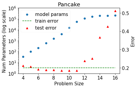
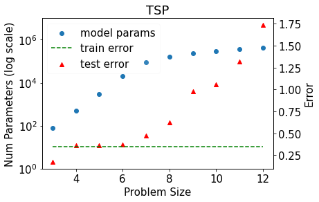
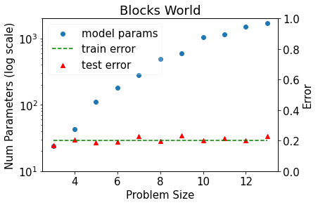
Figure 1: The minimum numbers of parameters (in log scale) required for fixed-depth neural networks to approximate the training sets with given loss thresholds (left) and the resulting losses on the test sets (right) as functions of the instance sizes. The loss threshold is 0.2, 0.35, and 0.2 for Pancake, TSP, and Blocks World, respectively.

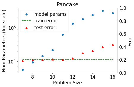
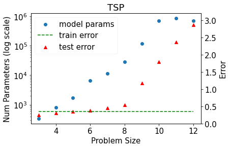
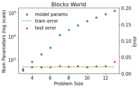
Figure 2: The minimum numbers of parameters (in log scale) required for fixed-width neural networks to approximate the training sets with given loss thresholds (left) and the resulting losses on the test sets (right) as functions of the instance sizes. The loss threshold is 0.1, 0.35, and 0.02 for Pancake, TSP, and Blocks World, respectively.

Experiment 1

Figure 1 shows the smallest numbers of parameters required for fixed-depth neural networks to approximate the training sets with given loss thresholds (in log scale) and the resulting losses on the test sets as functions of the instance sizes.

For Pancake and TSP, we first see linear trends for the number of parameters in log scale as their instance sizes increase (Phase 1), which suggests that the numbers of parameters increase exponentially in the instance sizes. We then see stagnations around Pancake instances of size 12 and TSP instances of size 7 (Phase 2). The losses on the test sets start to increase roughly at the point of stagnation. One explanation for the increasing losses on the test sets is that the training and test sets contain fewer and fewer common states as the instance sizes increase since the numbers of states increase with the instance sizes, and it thus becomes more and more unlikely that the same states will be part of both the training and test sets. Thus, the ability to generalize well to states not in the training set becomes more and more important, but the increasing losses on the test sets show that generalization is poor. The poor generalization could be due to overfitting the training sets, which we did not prevent in our experiments (other than by stopping training early) since we need to approximate the completely informed heuristic functions closely for all states, including those in the training sets. For Blocks World, we see only Phase 1 and thus cannot be sure whether it is followed by Phase 2 (overfitting). We tried to increase its instance sizes to ensure that it is not a counter example to our claims, but the generation of the training is not feasible given our available computing resources.

Figure 2 shows similar patterns for fixed-width neural networks although the graphs are noisier than those for fixed-depth neural networks since adding another hidden layer with $n$ neurons increases the number of parameters by $n^{2}+n$ and thus by more than for fixed-depth neural networks, resulting in less smooth graphs.

Overall, our results suggest that completely informed heuristic functions for our NP-hard minimum-cost path problems might not have the necessary structure to achieve sufficiently compressed representations of the completely informed heuristic functions needed to scale to large instance sizes. In our experiments, we keep the numbers of states in the training sets constant, which appears to make the sizes of the neural networks stagnate as the instance sizes increase but also prevents them from approximating the completely informed heuristic functions with high precision.

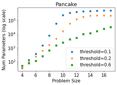
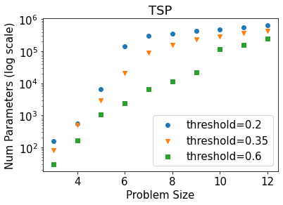
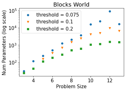
Figure 3: The minimum numbers of parameters (in log scale) required for fixed-depth neural networks to approximate the training sets with three loss thresholds each as functions of the instance sizes.

Experiment 2

So far, the loss thresholds were hand-selected for each problem. We now report experimental results for two additional loss thresholds per problem.

Figure 3 shows that larger loss thresholds for fixed-depth neural networks result in smaller numbers of parameters since it is easier to approximate functions with larger loss thresholds. However, our experimental results for the numbers of parameters are similar for all loss thresholds. Our conclusions of Experiment 1 thus continue to apply, namely that there are linear trends for the numbers of parameters in log scale (possibly followed by stagnations) as the instance sizes increase.

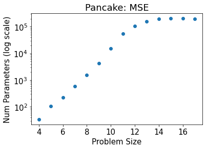
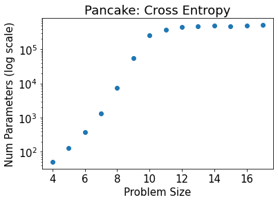
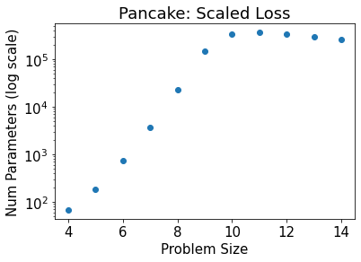
Figure 4: The minimum numbers of parameters (in log scale) required for fixed-depth neural networks to approximate the training sets for Pancake with given loss thresholds as functions of the instance sizes. The loss threshold of the MSE, cross entropy, and scaled loss is 0.2, 90%, and 0.001, respectively.

Experiment 3

So far, we treated the approximation of the training sets as a regression problem and used mean squared error as the loss function. We now report experimental results for two additional settings, namely 1) treating the problem as a classification problem and using the (categorical) cross-entropy loss as loss function, following (Ferber et al., 2020), and 2) using the “scaled" loss as loss function, defined as $\frac{1}{N}\sum_{i=1}^{N}\left(\frac{\hat{h}(s_{i})}{h^{*}(s_{i})}-1\right)^{2}$, where $N$ is the size of the training set and $s_{i}$ is the state of its $i$th element. The motivation behind the scaled loss is that the suboptimality factor of A* is governed by the relative error $\hat{h}(s_{i})/h^{*}(s_{i})-1$ rather than the absolute error $\hat{h}(s_{i})-h^{*}(s_{i})$ if $\hat{h}(s_{i})>h^{*}(s_{i})$ (Ebendt and Drechsler, 2009).

Figure 4 shows that our experimental results for the numbers of parameters of fixed-depth neural networks are similar for all loss functions. Our conclusions of Experiment 1 thus continue to apply, namely that there are linear trends for the numbers of parameters in log scale (possibly followed by stagnations) as the instance sizes increase.

6 Conclusion

We supported our claim that approaches that use universal function approximators to approximate completely informed heuristic functions with high precision to speed up A* searches for solving NP-hard minimum-cost path problems do not scale to large instance sizes. The research community might therefore want to investigate other ways of integrating heuristic search with machine learning.

Appendix A Summary of Previous Results

					Results of the Search
(Inst. Size) Problem	# States	Approach	# Parameters		Path Length		# Expanded States
48 Tile Puzzle	$3.00\times 10^{62}$	DeepCubeA		$3.00\times 10^{7}$		$253.4$		*$5.73\times 10^{6}$
24 Tile Puzzle	$7.70\times 10^{24}$	DeepCubeA	$\leq$	$2.10\times 10^{7}$	$\geq$	$89.5$	$\leq$	*$2.01\times 10^{6}$
		PHS*		$1.05\times 10^{6}$	$\leq$	$224.0$	$\geq$	$2.87\times 10^{3}$
		PHSh		$1.05\times 10^{6}$		$119.5$		$5.86\times 10^{4}$
		BLH	$\geq$	*$3.00\times 10^{4}$		-		$5.22\times 10^{6}$
15 Tile Puzzle	$1.00\times 10^{13}$	DeepCubeA	$\leq$	$1.82\times 10^{7}$		$52.0$	$\leq$	$*1.28\times 10^{6}$
		BLH	$\geq$	*$3.00\times 10^{4}$		-	$\geq$	$1.01\times 10^{4}$
Sokoban	*$1.53\times 10^{15}$	DeepCubeA	$\leq$	$1.50\times 10^{7}$	$\geq$	$32.9$	$\geq$	$1.05\times 10^{3}$
		PHS*	$\geq$	$3.71\times 10^{6}$		$37.6$		$1.52\times 10^{3}$
		PHSh	$\geq$	$3.71\times 10^{6}$	$\leq$	39.1	$\leq$	$2.13\times 10^{3}$

Table 1: Comparison of previous approaches: DeepCubeA [Agostinelli et al., 2019], Policy Guided Heuristic Search (PHS*, PHS_h) [Orseau and Lelis, 2021], and Bootstrap Learning Heuristic (BLH)  [Arfaee et al., 2010]. "-" denotes an unreported value in the original paper. "*" in front of a value denotes that it is an approximation based on additional assumptions. "$\leq$" in front of a value denotes that it is the worst observed value. "$\geq$" in front of a value denotes that it is the best observed value.

Table 1 shows a summary of some existing experimental results from the papers of previous approaches. We estimate the number of states of Sokoban on a $10\times 10$ grid with 4 boxes as $100\times{100\choose 4}\times{100\choose 4}$, which is the product of the numbers of possible player locations, possible start locations of the boxes, and possible goal locations of the boxes. We estimate the numbers of parameters of BLH by assuming neural networks with 2 hidden layers and 1,000 neurons per hidden layer. In general, we ignore all parameters of the batch normalization layers. Changing numbers of parameters for an approach result from changing numbers of inputs due to the changing instance sizes rather than any changes to the layouts of the neural networks. An exception is DeepCubeA, which uses 6 residual blocks [He et al., 2016] for Tile Puzzle and 4 residual blocks for Sokoban. We estimate the numbers of expanded states of DeepCubeA by dividing the reported numbers of generated states by the branching factors.

Our research was motivated by the observation that, for Tile Puzzle, DeepCubeA produces neural networks with larger numbers of parameters for larger instance sizes.

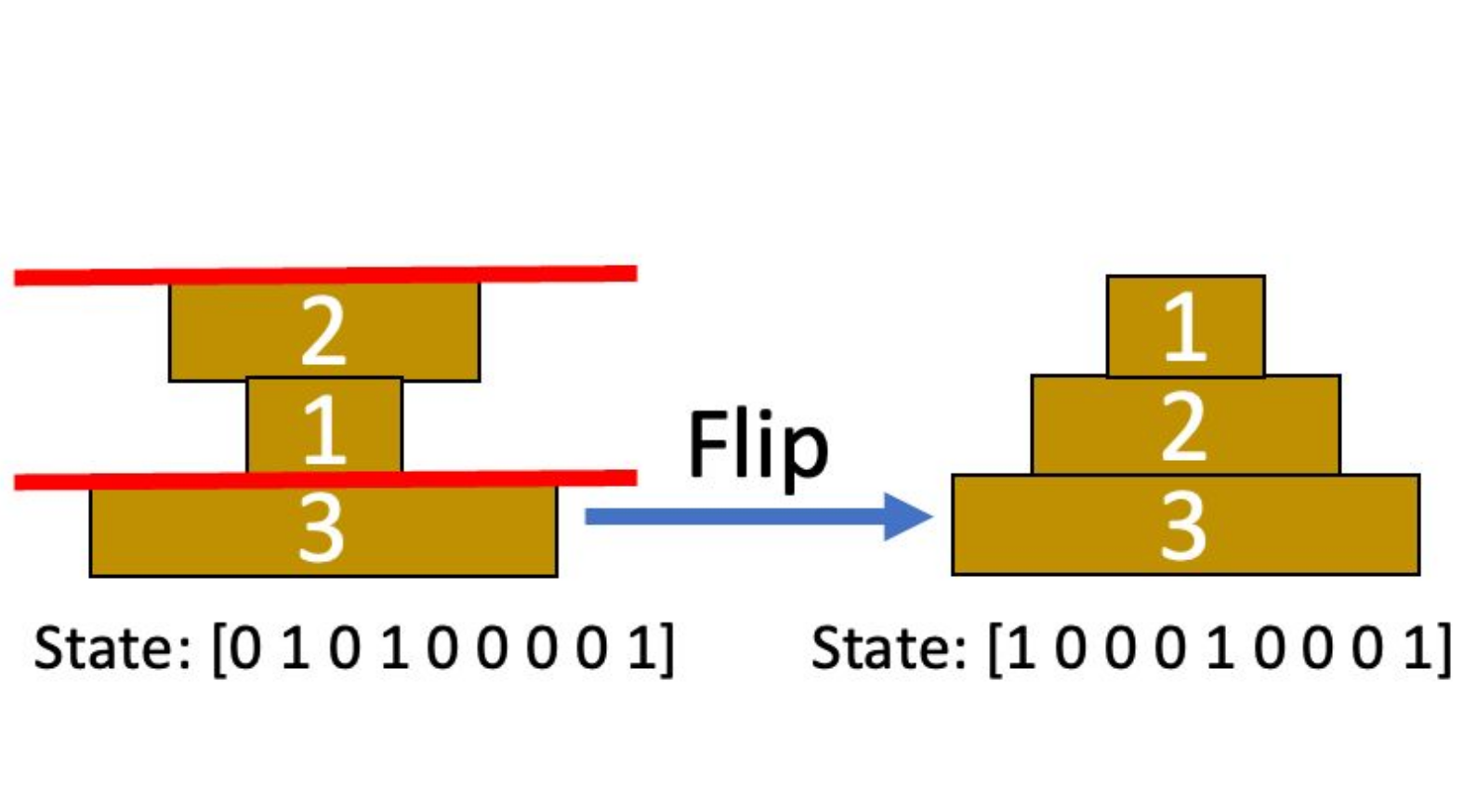
(a) Pancake

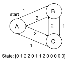
(b) TSP

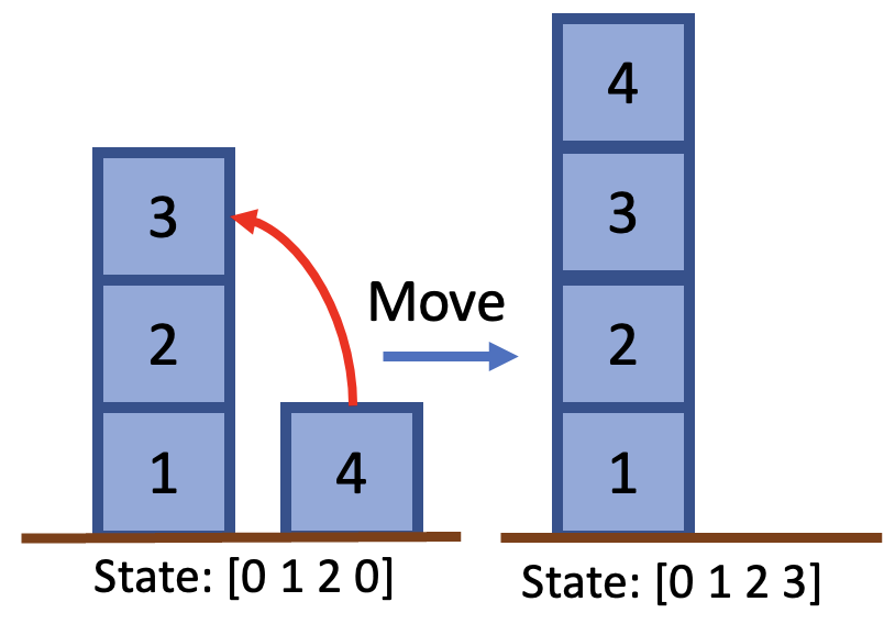
(c) Blocks World

Figure 5: States and their encodings for the three NP-hard minimum-cost path problems.

Appendix B Description of the NP-Hard Minimum-Cost Path Problems

Pancake

(1) Description: The pancake sorting problem ("Pancake") is NP-hard [Bulteau et al., 2015]. The task is to sort pancakes of different sizes, that are stacked on top of each other, with the minimum number of moves, each of which consists of inserting a spatula at any position in the stack and flipping (inverting) all pancakes above it. (2) Dataset Generation: We generate the training sets via a random walk from the goal states, following [Agostinelli et al., 2019]. We calculate the completely informed heuristic function values of the encountered states via an A* search with the consistent gap heuristic function [Helmert, 2010]. (3) Encoding: We encode a state via a one-hot encoding of the location of each pancake in the stack, as shown in Figure 5(a). (4) Properties 1 and 2: Pancake satisfies the properties for $\epsilon=1$ since the branching factor is the number of pancakes minus one, the number of edges in a minimum-cost path is at most twice the number of pancakes (since one can solve any Pancake instance by repeatedly bringing the largest pancake not in its correct position in the goal configuration to the top of the stack with one flip and then to its correct position in the goal configuration with another flip), and one minimizes the number of flips (meaning that each edge cost is one).

TSP

(1) Description: The asymmetric travelling salesperson problem ("TSP") is NP-hard [Cormen et al., 2009]. The task is to find a minimum-cost tour that visits every city. (2) Dataset Generation: We generate the training sets by considering (only) the start states of the searches (where the salesperson is still in the start city) of different TSP instances of the same instance size. We generate complete weighted directed graphs with the given number of cities and edge costs that are uniformly sampled from 0.1, 0.2 …50.0. We calculate the completely informed heuristic function values of the start states via the Held–Karp algorithm [Held and Karp, 1962]. (3) Encoding: We encode a state as a vector that encodes, for each edge, its cost and, for each city, whether it has already been visited or is currently visited, as shown in Figure 5(b). The first city listed is the start city. (4) Properties 1 and 2: Our version of TSP satisfies the properties for $\epsilon=0.1$ since the branching factor is the number of cities minus one, the number of edges in a minimum-cost path equals the number of cities, and each edge cost is a multiple of 0.1.

Blocks World

(1) Description: The Blocks World ("BW") problem is NP-hard  [Gupta and Nau, 1992], and we suspect that it remains NP-hard with the fixed goal configuration that we use. Several toy blocks, numbered $1\ldots n$, form stacks on a table top. The task is to transform a given start configuration of blocks into a given goal configuration with the minimum number of moves, each of which moves a block from the top of a stack to the top of another stack or the table. (2) Dataset Generation: We use the goal configurations where all blocks are stacked in order of their numbers in one stack, with block 1 at the bottom. We generate the training sets by randomly generating start configurations. We calculate their completely informed heuristic function values via an A* search with the consistent heuristic function given by the numbers of blocks that are directly on top of blocks or the table top that they are not directly on top of in the goal configuration. (3) Encoding: We encode a state as a vector that encodes, for each block, which block it is directly on top of (with 0 denoting the table top), following [Slaney and Thiébaux, 2001], as shown in Figure 5(c). (4) Properties 1 and 2: Blocks World satisfies the properties for $\epsilon=1$ since the branching factor grows quadratically in the number of blocks, the number of edges in a minimum-cost path is at most twice the number of blocks (since one can solve any Blocks World instance by first moving all blocks directly onto the table top and then to their correct positions in the goal configuration), and one minimizes the number of block moves (meaning that each edge cost is one).

References

- Agostinelli et al. [2019] Forest Agostinelli, Stephen McAleer, Alexander Shmakov, and Pierre Baldi. Solving the Rubik’s cube with deep reinforcement learning and search. Nature Machine Intelligence, 1(8):356–363, 2019.
- Agostinelli et al. [2021a] Forest Agostinelli, Stephen McAleer, Alexander Shmakov, Roy Fox, Marco Valtorta, Biplav Srivastava, and Pierre Baldi. Obtaining approximately admissible heuristic functions through deep reinforcement learning and A* search. Bridging the Gap between AI Planning and Reinforcement Learning workshop at International Conference on Automated Planning and Scheduling, 2021a.
- Agostinelli et al. [2021b] Forest Agostinelli, Alexander Shmakov, Stephen McAleer, Roy Fox, and Pierre Baldi. A* search without expansions: Learning heuristic functions with deep Q-networks. arXiv preprint arXiv:2102.04518, 2021b.
- Arfaee et al. [2010] Shahab Jabbari Arfaee, Sandra Zilles, and Robert Holte. Bootstrap learning of heuristic functions. In Annual Symposium on Combinatorial Search, 2010.
- Bruck and Goodman [1988] Jehoshua Bruck and Joseph Goodman. On the power of neural networks for solving hard problems. In Advances in Neural Information Processing Systems, 1988.
- Bulteau et al. [2015] Laurent Bulteau, Guillaume Fertin, and Irena Rusu. Pancake flipping is hard. Journal of Computer and System Sciences, 81(8):1556–1574, 2015.
- Cook [2003] Stephen Cook. The importance of the P versus NP question. Journal of the ACM, 50:27–29, 2003.
- Cormen et al. [2009] Thomas Cormen, Charles Leiserson, Ronald Rivest, and Clifford Stein. Introduction to algorithms. MIT press, 2009.
- Cybenko [1989] George Cybenko. Approximation by superpositions of a sigmoidal function. Mathematics of Control, Signals and Systems, 2(4):303–314, 1989.
- Ebendt and Drechsler [2009] Rüdiger Ebendt and Rolf Drechsler. Weighted A* search – unifying view and application. Artificial Intelligence, 173(14):1310–1342, 2009.
- Felner et al. [2018] Ariel Felner, Jiaoyang Li, Eli Boyarski, Hang Ma, Liron Cohen, TK Satish Kumar, and Sven Koenig. Adding heuristics to conflict-based search for multi-agent path finding. In International Conference on Automated Planning and Scheduling, 2018.
- Ferber et al. [2020] Patrick Ferber, Malte Helmert, and Jörg Hoffmann. Neural network heuristics for classical planning: A study of hyperparameter space. In ECAI 2020, pages 2346–2353. IOS Press, 2020.
- Fitzpatrick et al. [2021] James Fitzpatrick, Deepak Ajwani, and Paula Carroll. Learning to sparsify travelling salesman problem instances. In International Conference on the Integration of Constraint Programming, Artificial Intelligence, and Operations Research, 2021.
- Goldenberg et al. [2014] Meir Goldenberg, Ariel Felner, Roni Stern, Guni Sharon, Nathan Sturtevant, Robert Holte, and Jonathan Schaeffer. Enhanced partial expansion A*. Journal of Artificial Intelligence Research, 50:141–187, 2014.
- Gupta and Nau [1992] Naresh Gupta and Dana Nau. On the complexity of blocks-world planning. Artificial Intelligence, 56(2-3):223–254, 1992.
- Hart et al. [1968] Peter Hart, Nils Nilsson, and Bertram Raphael. A formal basis for the heuristic determination of minimum cost paths. IEEE Transactions on Systems Science and Cybernetics, 4(2):100–107, 1968.
- He et al. [2016] Kaiming He, Xiangyu Zhang, Shaoqing Ren, and Jian Sun. Deep residual learning for image recognition. In IEEE Conference on Computer Vision and Pattern Recognition, 2016.
- Held and Karp [1962] Michael Held and Richard Karp. A dynamic programming approach to sequencing problems. Journal of the Society for Industrial and Applied Mathematics, 10(1):196–210, 1962.
- Helmert [2010] Malte Helmert. Landmark heuristics for the pancake problem. In Annual Symposium on Combinatorial Search, 2010.
- Helmert and Mattmüller [2008] Malte Helmert and Robert Mattmüller. Accuracy of admissible heuristic functions in selected planning domains. In National Conference on Artificial Intelligence, pages 938–943, 2008.
- Helmert and Röger [2008] Malte Helmert and Gabriele Röger. How good is almost perfect? In National Conference on Artificial Intelligence, 2008.
- Higgins [2021] Irina Higgins. Generalizing universal function approximators. Nature Machine Intelligence, 3(3):192–193, 2021.
- Hornik et al. [1989] Kurt Hornik, Maxwell Stinchcombe, and Halbert White. Multilayer feedforward networks are universal approximators. Neural Networks, 2(5):359–366, 1989.
- Ioffe and Szegedy [2015] Sergey Ioffe and Christian Szegedy. Batch normalization: Accelerating deep network training by reducing internal covariate shift. In International Conference on Machine Learning, 2015.
- Kidger and Lyons [2020] Patrick Kidger and Terry Lyons. Universal approximation with deep narrow networks. In Conference on Learning Theory, 2020.
- Kingma and Ba [2015] Diederick Kingma and Jimmy Ba. Adam: A method for stochastic optimization. In International Conference on Learning Representations, 2015.
- Lin and Jegelka [2018] Hongzhou Lin and Stefanie Jegelka. Resnet with one-neuron hidden layers is a universal approximator. Advances in Neural Information Processing Systems, 2018.
- McAleer et al. [2018] Stephen McAleer, Forest Agostinelli, Alexander Shmakov, and Pierre Baldi. Solving the Rubik’s cube with approximate policy iteration. In International Conference on Learning Representations, 2018.
- Nair and Hinton [2010] Vinod Nair and Geoffrey Hinton. Rectified linear units improve restricted Boltzmann machines. In International Conference on Machine Learning, 2010.
- Orseau and Lelis [2021] Laurent Orseau and Levi Lelis. Policy-guided heuristic search with guarantees. In AAAI Conference on Artificial Intelligence, 2021.
- Orseau et al. [2018] Laurent Orseau, Levi Lelis, Tor Lattimore, and Théophane Weber. Single-agent policy tree search with guarantees. Advances in Neural Information Processing Systems, 2018.
- Papadimitriou and Steiglitz [1998] Christos Papadimitriou and Kenneth Steiglitz. Combinatorial optimization: Algorithms and complexity. Courier Corporation, 1998.
- Pearl [1984] Judea Pearl. Heuristics: Intelligent search strategies for computer problem solving. Addison-Wesley, 1984.
- Pendurkar et al. [2022] Sumedh Pendurkar, Taoan Huang, Sven Koenig, and Guni Sharon. A discussion on the scalability of heuristic approximators. In Annual Symposium on Combinatorial Search, 2022.
- Pinkus [1999] Allan Pinkus. Approximation theory of the MLP model in neural networks. Acta Numerica, 8:143–195, 1999.
- Ratner and Warmuth [1990] Daniel Ratner and Manfred Warmuth. The ()-puzzle and related relocation problems. Journal of Symbolic Computation, 10(2):111–137, 1990.
- Slaney and Thiébaux [2001] John Slaney and Sylvie Thiébaux. Blocks world revisited. Artificial Intelligence, 125(1-2):119–153, 2001.
- Sonoda and Murata [2017] Sho Sonoda and Noboru Murata. Neural network with unbounded activation functions is universal approximator. Applied and Computational Harmonic Analysis, 43(2):233–268, 2017.
- Valenzano and Yang [2017] Richard Anthony Valenzano and Danniel Sihui Yang. An analysis and enhancement of the gap heuristic for the pancake puzzle. In Annual Symposium on Combinatorial Search, 2017.